Embed Size (px)
Citation preview
“There’s nothing to fear but the fear itself.That’s called recursion, and that would lead you
to infinite fear.”

Hello, human! Welcome to my book on Python and algorithms! If you
are reading this you probably agree with me that those two can be a
lot of fun together (or you might be lost, and in this case I
suggest you give it a try anyway!). Also, many of the examples
shown here are available in my git repository, together with several
other (more advanced) examples for abstract data structures, trees,
graphs, and solutions for the Euler Project and the Topcoder
website. Don’t forget to check them out!
This text was written purely for fun (I know, I know, this is a
broad definition of the word fun...) with no pretensions for
anything big, so please forgive me (or better, let me know) if you
find any typo or mistake. I am not a computer scientist by
formation (I am actually an almost-I-swear-it-is-close-Ph.D. in
Physics) so this maybe makes things a little less usual (or risky?).
I hope you have fun!
Mari, Stony Brook, NY
Summer/2013

4
Contents
I Flying with Python 9
1 Numbers 111.1 Integers . . . . . . . . . . . . . . . . . . . . . . . . . . . . . . 111.2 Floats . . . . . . . . . . . . . . . . . . . . . . . . . . . . . . . 121.3 Complex Numbers . . . . . . . . . . . . . . . . . . . . . . . . 131.4 The fractions Module . . . . . . . . . . . . . . . . . . . . . 141.5 The decimal Module . . . . . . . . . . . . . . . . . . . . . . . 151.6 Other Representations . . . . . . . . . . . . . . . . . . . . . . 151.7 Additional Exercises . . . . . . . . . . . . . . . . . . . . . . . 16
2 Built-in Sequence Types 252.1 Strings . . . . . . . . . . . . . . . . . . . . . . . . . . . . . . . 272.2 Tuples . . . . . . . . . . . . . . . . . . . . . . . . . . . . . . . 332.3 Lists . . . . . . . . . . . . . . . . . . . . . . . . . . . . . . . . 352.4 Bytes and Byte Arrays . . . . . . . . . . . . . . . . . . . . . . 43
3 Collection Data Structures 453.1 Sets . . . . . . . . . . . . . . . . . . . . . . . . . . . . . . . . 453.2 Dictionaries . . . . . . . . . . . . . . . . . . . . . . . . . . . . 493.3 Python’s collection Data Types . . . . . . . . . . . . . . . 543.4 Additional Exercises . . . . . . . . . . . . . . . . . . . . . . . 58
4 Python’s Structure and Modules 634.1 Modules in Python . . . . . . . . . . . . . . . . . . . . . . . . 634.2 Control Flow . . . . . . . . . . . . . . . . . . . . . . . . . . . 664.3 File Handling . . . . . . . . . . . . . . . . . . . . . . . . . . . 724.4 Multiprocessing and Threading . . . . . . . . . . . . . . . . . 794.5 Error Handling in Python . . . . . . . . . . . . . . . . . . . . 814.6 Debugging and Profiling . . . . . . . . . . . . . . . . . . . . . 83
5
6 CONTENTS
4.7 Unit Testing . . . . . . . . . . . . . . . . . . . . . . . . . . . . 86
5 Object-Oriented Design 895.1 Classes and Objects . . . . . . . . . . . . . . . . . . . . . . . 905.2 Principles of OOP . . . . . . . . . . . . . . . . . . . . . . . . 915.3 Python Design Patterns . . . . . . . . . . . . . . . . . . . . . 945.4 Additional Exercises . . . . . . . . . . . . . . . . . . . . . . . 96
II Algorithms are Fun 99
6 Additional Abstract Data Structures 1016.1 Stacks . . . . . . . . . . . . . . . . . . . . . . . . . . . . . . . 1016.2 Queues . . . . . . . . . . . . . . . . . . . . . . . . . . . . . . . 1046.3 Deques . . . . . . . . . . . . . . . . . . . . . . . . . . . . . . . 1086.4 Priority Queues and Heaps . . . . . . . . . . . . . . . . . . . 1106.5 Linked Lists . . . . . . . . . . . . . . . . . . . . . . . . . . . . 1146.6 Additional Exercises . . . . . . . . . . . . . . . . . . . . . . . 120
7 Asymptotic Analysis 1337.1 Complexity Classes . . . . . . . . . . . . . . . . . . . . . . . . 1337.2 Recursion . . . . . . . . . . . . . . . . . . . . . . . . . . . . . 1357.3 Runtime in Functions . . . . . . . . . . . . . . . . . . . . . . 136
8 Sorting 1398.1 Quadratic Sort . . . . . . . . . . . . . . . . . . . . . . . . . . 1398.2 Linear Sort . . . . . . . . . . . . . . . . . . . . . . . . . . . . 1428.3 Loglinear Sort . . . . . . . . . . . . . . . . . . . . . . . . . . . 1428.4 Comparison Between Sorting Methods . . . . . . . . . . . . . 1488.5 Additional Exercises . . . . . . . . . . . . . . . . . . . . . . . 149
9 Searching 1539.1 Sequential Search . . . . . . . . . . . . . . . . . . . . . . . . . 1539.2 Binary Search . . . . . . . . . . . . . . . . . . . . . . . . . . . 1549.3 Additional Exercises . . . . . . . . . . . . . . . . . . . . . . . 156
10 Dynamic Programming 16310.1 Memoization . . . . . . . . . . . . . . . . . . . . . . . . . . . 16310.2 Additional Exercises . . . . . . . . . . . . . . . . . . . . . . . 165
CONTENTS 7
III Climbing Graphs and Trees 169
11 Introduction to Graphs 17111.1 Basic Definitions . . . . . . . . . . . . . . . . . . . . . . . . . 17111.2 The Neighborhood Function . . . . . . . . . . . . . . . . . . . 17311.3 Introduction to Trees . . . . . . . . . . . . . . . . . . . . . . . 176
12 Binary Trees 17912.1 Basic Concepts . . . . . . . . . . . . . . . . . . . . . . . . . . 17912.2 Representing Binary Trees . . . . . . . . . . . . . . . . . . . . 17912.3 Binary Search Trees . . . . . . . . . . . . . . . . . . . . . . . 18312.4 Self-Balancing BST . . . . . . . . . . . . . . . . . . . . . . . . 18612.5 Additional Exercises . . . . . . . . . . . . . . . . . . . . . . . 193
13 Traversals and Problems on Graphs and Trees 20713.1 Depth-First Search . . . . . . . . . . . . . . . . . . . . . . . . 20713.2 Breadth-First Search . . . . . . . . . . . . . . . . . . . . . . 20813.3 Representing Tree Traversals . . . . . . . . . . . . . . . . . . 20913.4 Additional Exercises . . . . . . . . . . . . . . . . . . . . . . . 211

8 CONTENTS
Part I
Flying with Python
9

Chapter 1
Numbers
When you learn a new language, the first thing you usually do (after ourdear ’hello world’) is to play with some arithmetic operations. Numberscan be integers, float point number, or complex. They are usually givendecimal representation but can be represented in any bases such as binary,hexadecimal, octahedral. In this section we will learn how Python dealswith numbers.
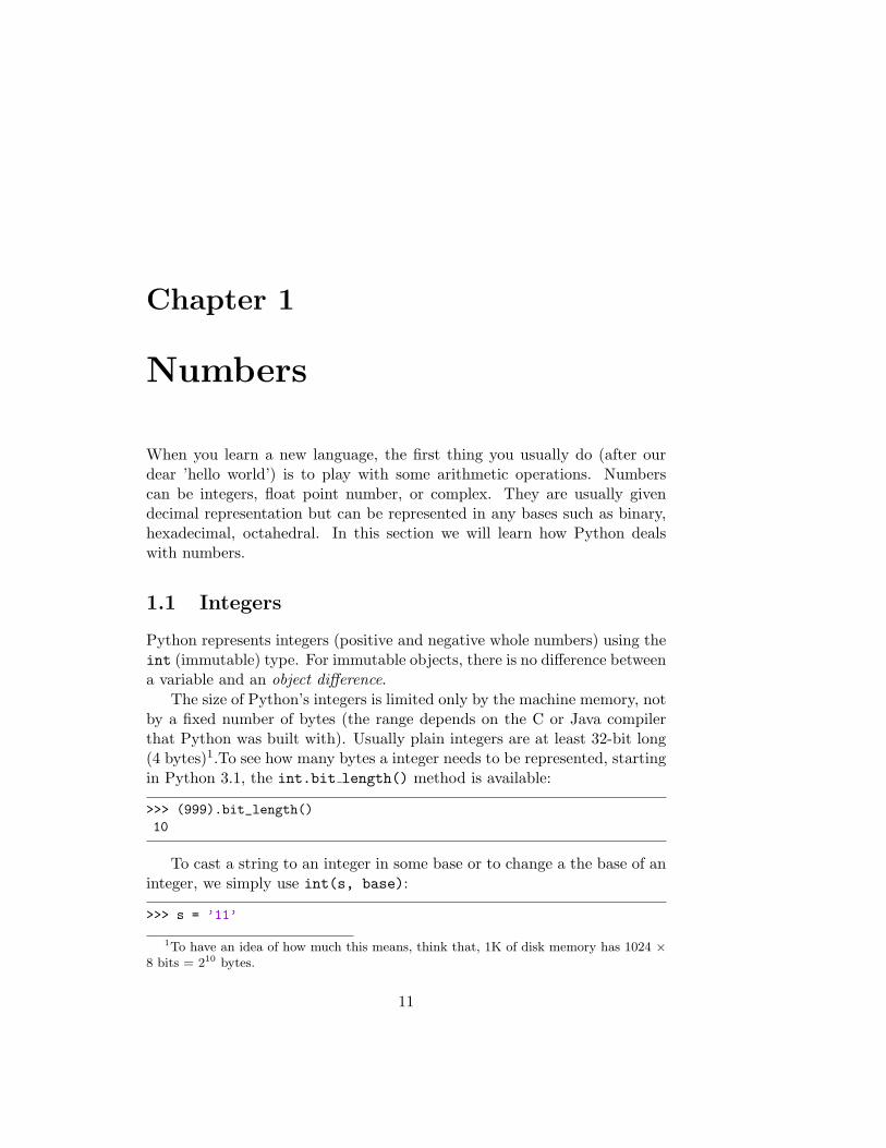
1.1 Integers
Python represents integers (positive and negative whole numbers) using theint (immutable) type. For immutable objects, there is no difference betweena variable and an object difference.
The size of Python’s integers is limited only by the machine memory, notby a fixed number of bytes (the range depends on the C or Java compilerthat Python was built with). Usually plain integers are at least 32-bit long(4 bytes)1.To see how many bytes a integer needs to be represented, startingin Python 3.1, the int.bit length() method is available:
>>> (999).bit_length()10
To cast a string to an integer in some base or to change a the base of aninteger, we simply use int(s, base):
>>> s = ’11’
1To have an idea of how much this means, think that, 1K of disk memory has 1024 ×8 bits = 210 bytes.
11
12 CHAPTER 1. NUMBERS
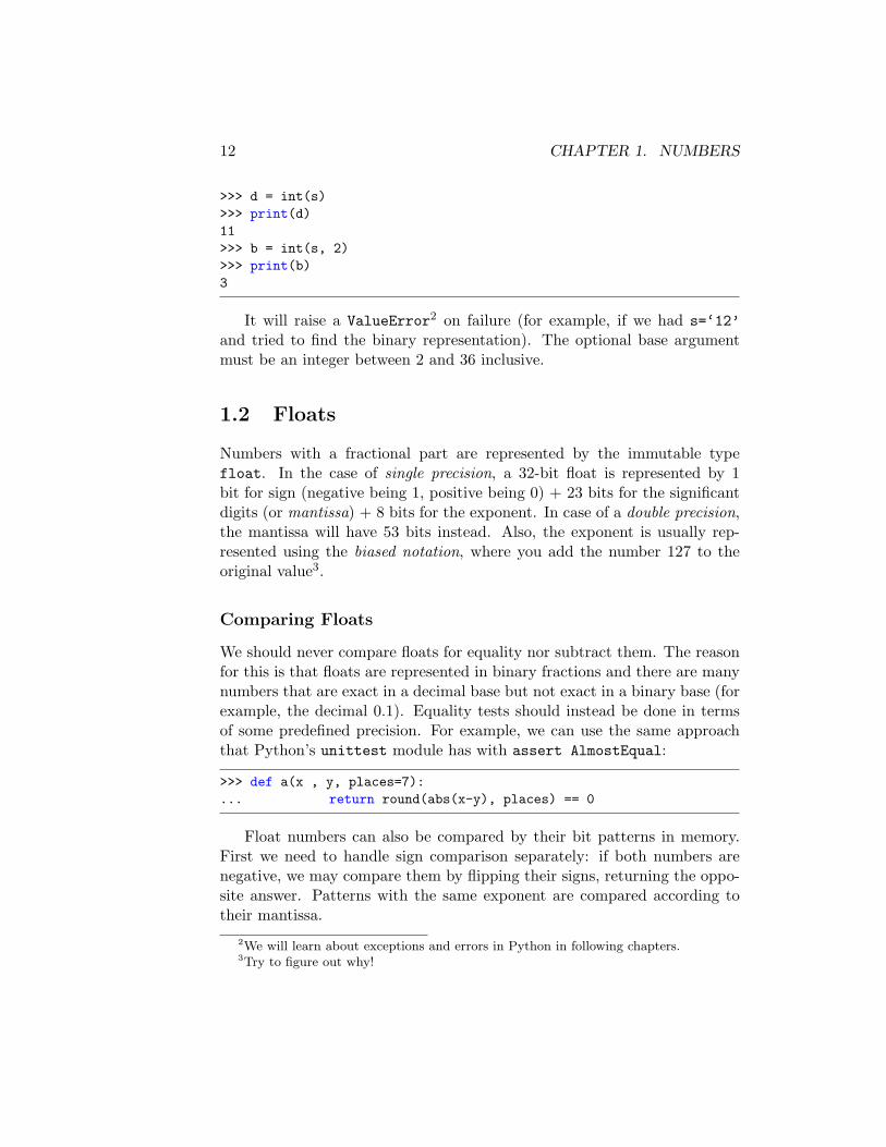
>>> d = int(s)>>> print(d)11>>> b = int(s, 2)>>> print(b)3
It will raise a ValueError2 on failure (for example, if we had s=‘12’and tried to find the binary representation). The optional base argumentmust be an integer between 2 and 36 inclusive.
1.2 Floats
Numbers with a fractional part are represented by the immutable typefloat. In the case of single precision, a 32-bit float is represented by 1bit for sign (negative being 1, positive being 0) + 23 bits for the significantdigits (or mantissa) + 8 bits for the exponent. In case of a double precision,the mantissa will have 53 bits instead. Also, the exponent is usually rep-resented using the biased notation, where you add the number 127 to theoriginal value3.
Comparing Floats
We should never compare floats for equality nor subtract them. The reasonfor this is that floats are represented in binary fractions and there are manynumbers that are exact in a decimal base but not exact in a binary base (forexample, the decimal 0.1). Equality tests should instead be done in termsof some predefined precision. For example, we can use the same approachthat Python’s unittest module has with assert AlmostEqual:
>>> def a(x , y, places=7):... return round(abs(x-y), places) == 0
Float numbers can also be compared by their bit patterns in memory.First we need to handle sign comparison separately: if both numbers arenegative, we may compare them by flipping their signs, returning the oppo-site answer. Patterns with the same exponent are compared according totheir mantissa.
2We will learn about exceptions and errors in Python in following chapters.3Try to figure out why!
1.3. COMPLEX NUMBERS 13
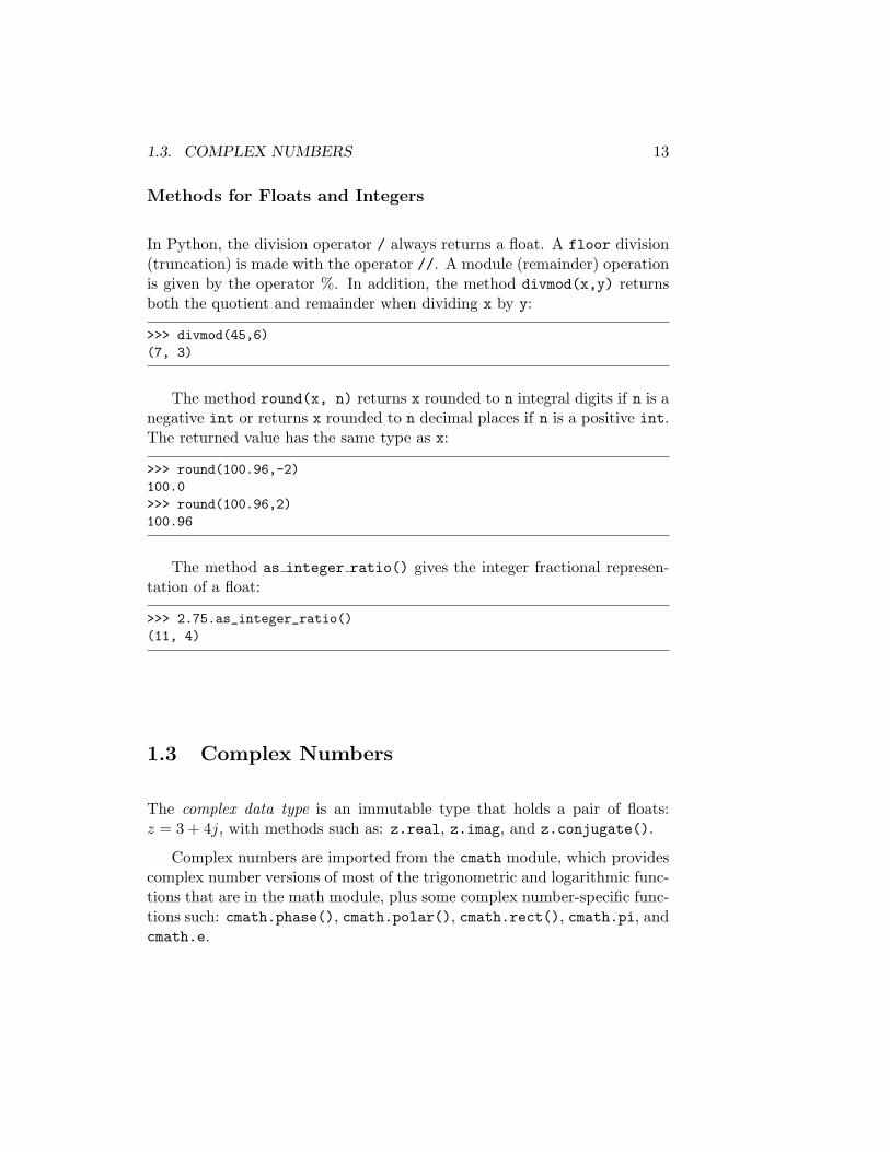
Methods for Floats and Integers
In Python, the division operator / always returns a float. A floor division(truncation) is made with the operator //. A module (remainder) operationis given by the operator %. In addition, the method divmod(x,y) returnsboth the quotient and remainder when dividing x by y:
>>> divmod(45,6)(7, 3)
The method round(x, n) returns x rounded to n integral digits if n is anegative int or returns x rounded to n decimal places if n is a positive int.The returned value has the same type as x:
>>> round(100.96,-2)100.0>>> round(100.96,2)100.96
The method as integer ratio() gives the integer fractional represen-tation of a float:
>>> 2.75.as_integer_ratio()(11, 4)
1.3 Complex Numbers
The complex data type is an immutable type that holds a pair of floats:z = 3 + 4j, with methods such as: z.real, z.imag, and z.conjugate().
Complex numbers are imported from the cmath module, which providescomplex number versions of most of the trigonometric and logarithmic func-tions that are in the math module, plus some complex number-specific func-tions such: cmath.phase(), cmath.polar(), cmath.rect(), cmath.pi, andcmath.e.
14 CHAPTER 1. NUMBERS
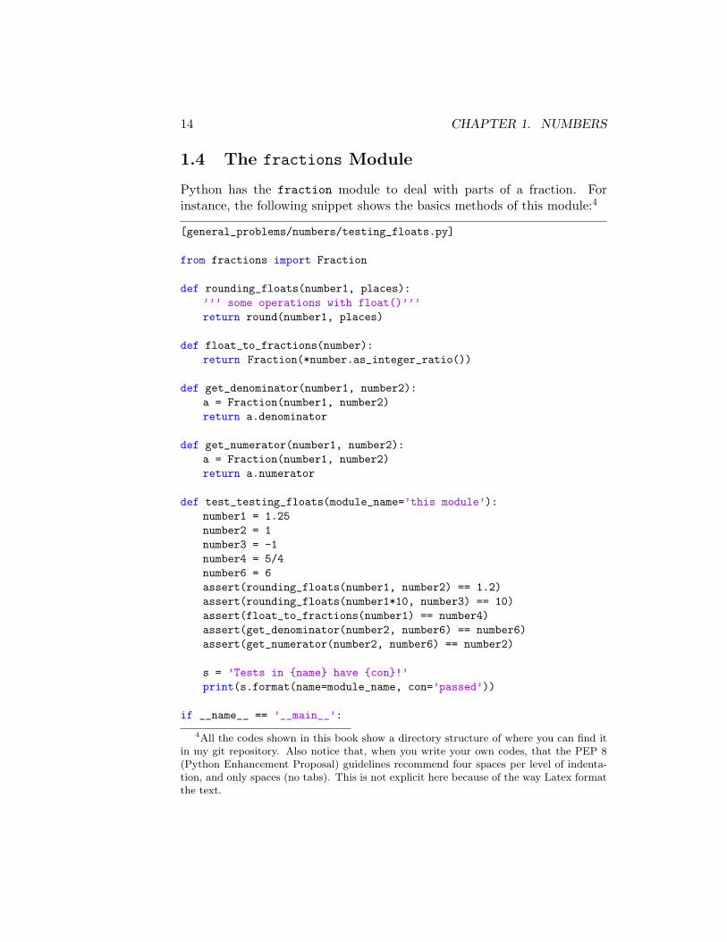
1.4 The fractions Module
Python has the fraction module to deal with parts of a fraction. Forinstance, the following snippet shows the basics methods of this module:4
[general_problems/numbers/testing_floats.py]
from fractions import Fraction
def rounding_floats(number1, places):’’’ some operations with float()’’’return round(number1, places)
def float_to_fractions(number):return Fraction(*number.as_integer_ratio())
def get_denominator(number1, number2):a = Fraction(number1, number2)return a.denominator
def get_numerator(number1, number2):a = Fraction(number1, number2)return a.numerator
def test_testing_floats(module_name=’this module’):number1 = 1.25number2 = 1number3 = -1number4 = 5/4number6 = 6assert(rounding_floats(number1, number2) == 1.2)assert(rounding_floats(number1*10, number3) == 10)assert(float_to_fractions(number1) == number4)assert(get_denominator(number2, number6) == number6)assert(get_numerator(number2, number6) == number2)
s = ’Tests in {name} have {con}!’print(s.format(name=module_name, con=’passed’))
if __name__ == ’__main__’:
4All the codes shown in this book show a directory structure of where you can find itin my git repository. Also notice that, when you write your own codes, that the PEP 8(Python Enhancement Proposal) guidelines recommend four spaces per level of indenta-tion, and only spaces (no tabs). This is not explicit here because of the way Latex formatthe text.
1.5. THE DECIMAL MODULE 15
test_testing_floats()
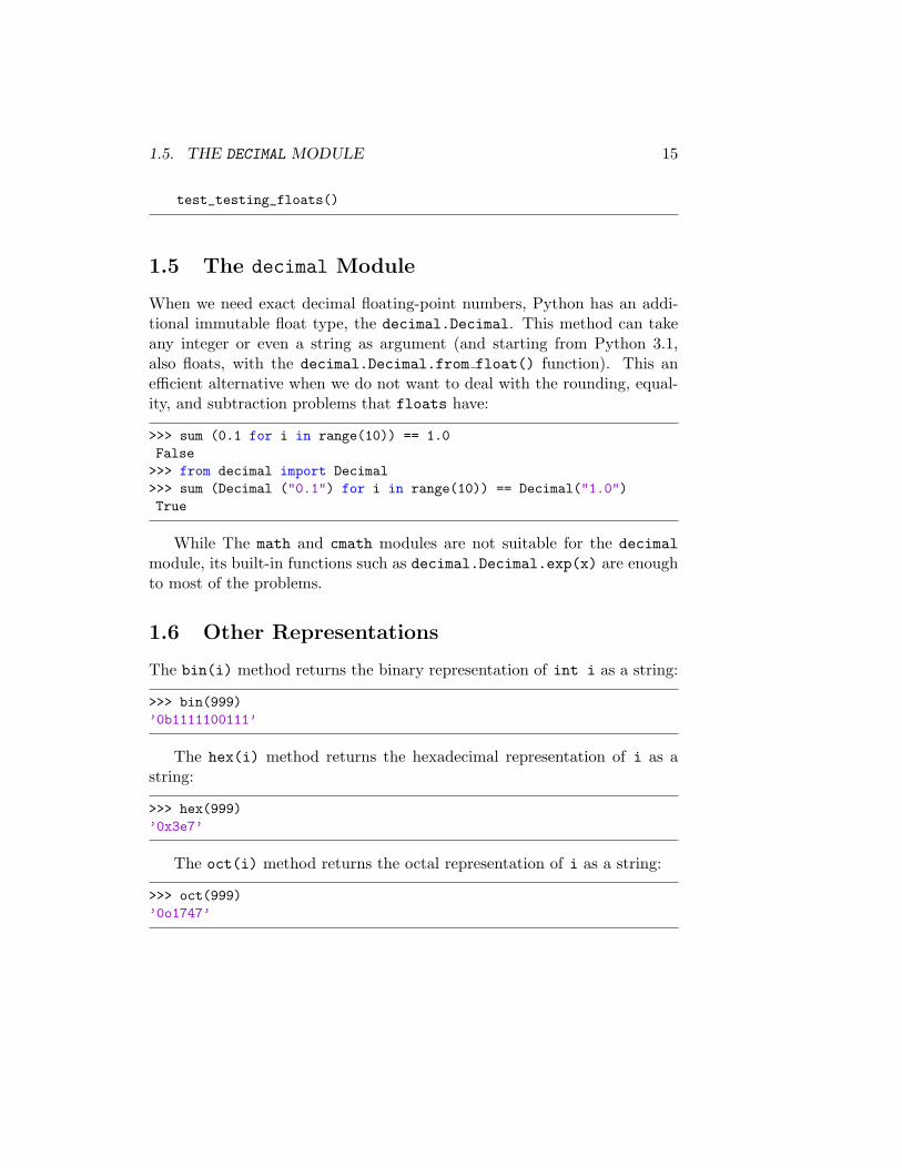
1.5 The decimal Module
When we need exact decimal floating-point numbers, Python has an addi-tional immutable float type, the decimal.Decimal. This method can takeany integer or even a string as argument (and starting from Python 3.1,also floats, with the decimal.Decimal.from float() function). This anefficient alternative when we do not want to deal with the rounding, equal-ity, and subtraction problems that floats have:
>>> sum (0.1 for i in range(10)) == 1.0False>>> from decimal import Decimal>>> sum (Decimal ("0.1") for i in range(10)) == Decimal("1.0")True
While The math and cmath modules are not suitable for the decimalmodule, its built-in functions such as decimal.Decimal.exp(x) are enoughto most of the problems.
1.6 Other Representations
The bin(i) method returns the binary representation of int i as a string:
>>> bin(999)’0b1111100111’
The hex(i) method returns the hexadecimal representation of i as astring:
>>> hex(999)’0x3e7’
The oct(i) method returns the octal representation of i as a string:
>>> oct(999)’0o1747’
16 CHAPTER 1. NUMBERS
1.7 Additional Exercises
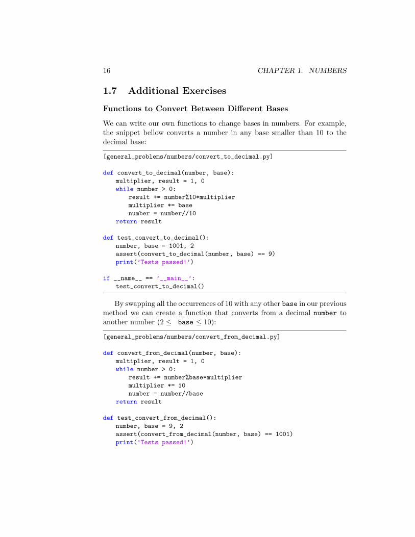
Functions to Convert Between Different Bases
We can write our own functions to change bases in numbers. For example,the snippet bellow converts a number in any base smaller than 10 to thedecimal base:
[general_problems/numbers/convert_to_decimal.py]
def convert_to_decimal(number, base):multiplier, result = 1, 0while number > 0:
result += number%10*multipliermultiplier *= basenumber = number//10
return result
def test_convert_to_decimal():number, base = 1001, 2assert(convert_to_decimal(number, base) == 9)print(’Tests passed!’)
if __name__ == ’__main__’:test_convert_to_decimal()
By swapping all the occurrences of 10 with any other base in our previousmethod we can create a function that converts from a decimal number toanother number (2 ≤ base ≤ 10):
[general_problems/numbers/convert_from_decimal.py]
def convert_from_decimal(number, base):multiplier, result = 1, 0while number > 0:
result += number%base*multipliermultiplier *= 10number = number//base
return result
def test_convert_from_decimal():number, base = 9, 2assert(convert_from_decimal(number, base) == 1001)print(’Tests passed!’)
1.7. ADDITIONAL EXERCISES 17
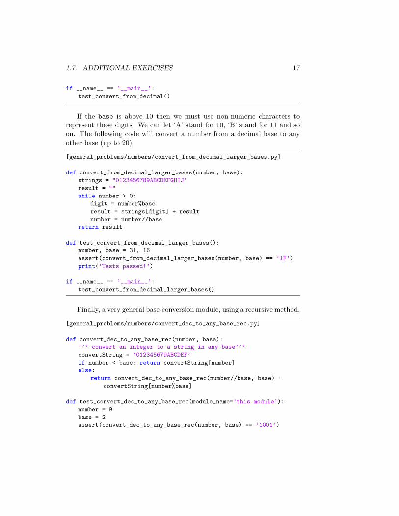
if __name__ == ’__main__’:test_convert_from_decimal()
If the base is above 10 then we must use non-numeric characters torepresent these digits. We can let ‘A’ stand for 10, ‘B’ stand for 11 and soon. The following code will convert a number from a decimal base to anyother base (up to 20):
[general_problems/numbers/convert_from_decimal_larger_bases.py]
def convert_from_decimal_larger_bases(number, base):strings = "0123456789ABCDEFGHIJ"result = ""while number > 0:
digit = number%baseresult = strings[digit] + resultnumber = number//base
return result
def test_convert_from_decimal_larger_bases():number, base = 31, 16assert(convert_from_decimal_larger_bases(number, base) == ’1F’)print(’Tests passed!’)
if __name__ == ’__main__’:test_convert_from_decimal_larger_bases()
Finally, a very general base-conversion module, using a recursive method:
[general_problems/numbers/convert_dec_to_any_base_rec.py]
def convert_dec_to_any_base_rec(number, base):’’’ convert an integer to a string in any base’’’convertString = ’012345679ABCDEF’if number < base: return convertString[number]else:
return convert_dec_to_any_base_rec(number//base, base) +convertString[number%base]
def test_convert_dec_to_any_base_rec(module_name=’this module’):number = 9base = 2assert(convert_dec_to_any_base_rec(number, base) == ’1001’)
18 CHAPTER 1. NUMBERS
s = ’Tests in {name} have {con}!’print(s.format(name=module_name, con=’passed’))
if __name__ == ’__main__’:test_convert_dec_to_any_base_rec()
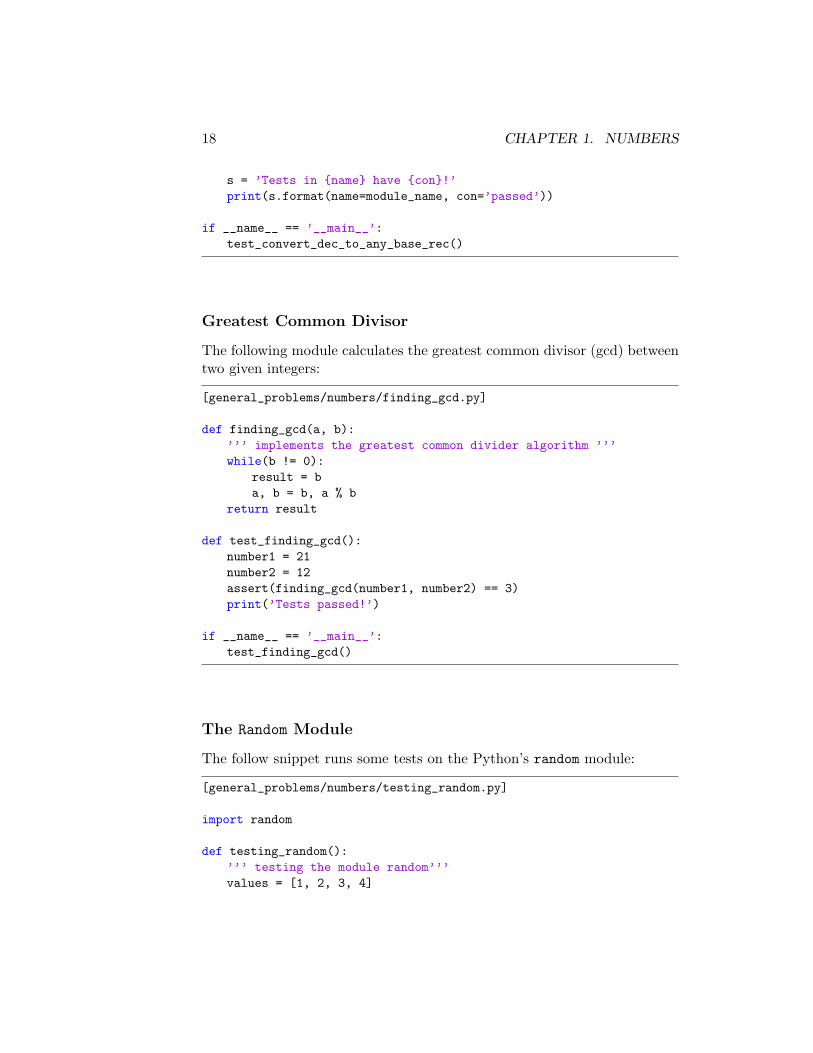
Greatest Common Divisor
The following module calculates the greatest common divisor (gcd) betweentwo given integers:
[general_problems/numbers/finding_gcd.py]
def finding_gcd(a, b):’’’ implements the greatest common divider algorithm ’’’while(b != 0):
result = ba, b = b, a % b
return result
def test_finding_gcd():number1 = 21number2 = 12assert(finding_gcd(number1, number2) == 3)print(’Tests passed!’)
if __name__ == ’__main__’:test_finding_gcd()
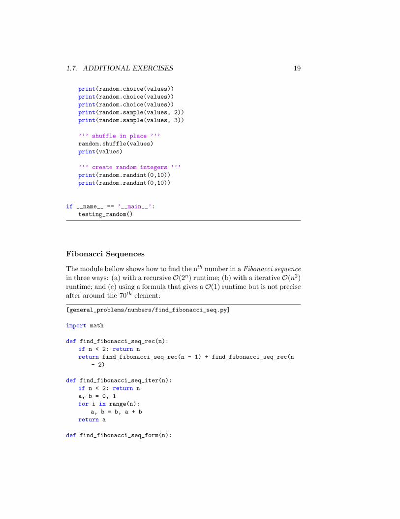
The Random Module
The follow snippet runs some tests on the Python’s random module:
[general_problems/numbers/testing_random.py]
import random
def testing_random():’’’ testing the module random’’’values = [1, 2, 3, 4]
1.7. ADDITIONAL EXERCISES 19
print(random.choice(values))print(random.choice(values))print(random.choice(values))print(random.sample(values, 2))print(random.sample(values, 3))
’’’ shuffle in place ’’’random.shuffle(values)print(values)
’’’ create random integers ’’’print(random.randint(0,10))print(random.randint(0,10))
if __name__ == ’__main__’:testing_random()
Fibonacci Sequences
The module bellow shows how to find the nth number in a Fibonacci sequencein three ways: (a) with a recursive O(2n) runtime; (b) with a iterative O(n2)runtime; and (c) using a formula that gives a O(1) runtime but is not preciseafter around the 70th element:
[general_problems/numbers/find_fibonacci_seq.py]
import math
def find_fibonacci_seq_rec(n):if n < 2: return nreturn find_fibonacci_seq_rec(n - 1) + find_fibonacci_seq_rec(n
- 2)
def find_fibonacci_seq_iter(n):if n < 2: return na, b = 0, 1for i in range(n):
a, b = b, a + breturn a
def find_fibonacci_seq_form(n):
20 CHAPTER 1. NUMBERS
sq5 = math.sqrt(5)phi = (1 + sq5) / 2return int(math.floor(phi ** n / sq5))
def test_find_fib():n = 10assert(find_fibonacci_seq_rec(n) == 55)assert(find_fibonacci_seq_iter(n) == 55)assert(find_fibonacci_seq_form(n) == 55)print(’Tests passed!’)
if __name__ == ’__main__’:test_find_fib()
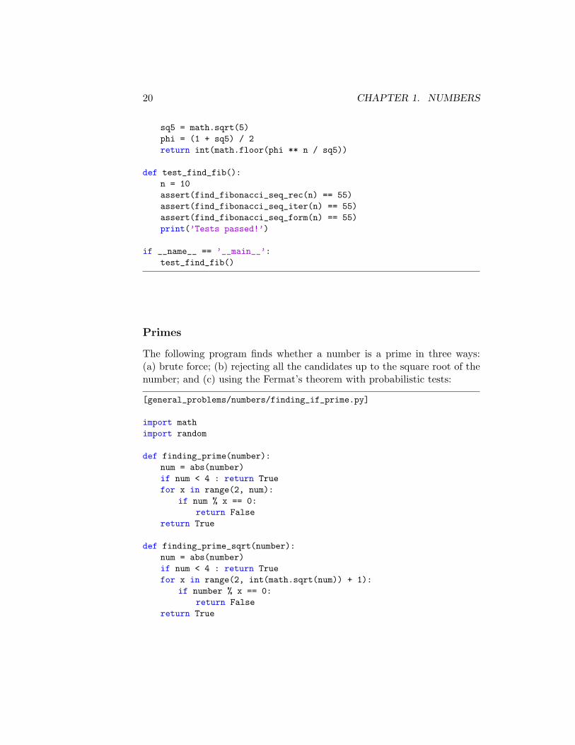
Primes
The following program finds whether a number is a prime in three ways:(a) brute force; (b) rejecting all the candidates up to the square root of thenumber; and (c) using the Fermat’s theorem with probabilistic tests:
[general_problems/numbers/finding_if_prime.py]
import mathimport random
def finding_prime(number):num = abs(number)if num < 4 : return Truefor x in range(2, num):
if num % x == 0:return False
return True
def finding_prime_sqrt(number):num = abs(number)if num < 4 : return Truefor x in range(2, int(math.sqrt(num)) + 1):
if number % x == 0:return False
return True
1.7. ADDITIONAL EXERCISES 21
def finding_prime_fermat(number):if number <= 102:
for a in range(2, number):if pow(a, number- 1, number) != 1:
return Falsereturn True
else:for i in range(100):
a = random.randint(2, number - 1)if pow(a, number - 1, number) != 1:
return Falsereturn True
def test_finding_prime():number1 = 17number2 = 20assert(finding_prime(number1) == True)assert(finding_prime(number2) == False)assert(finding_prime_sqrt(number1) == True)assert(finding_prime_sqrt(number2) == False)assert(finding_prime_fermat(number1) == True)assert(finding_prime_fermat(number2) == False)print(’Tests passed!’)
if __name__ == ’__main__’:test_finding_prime()
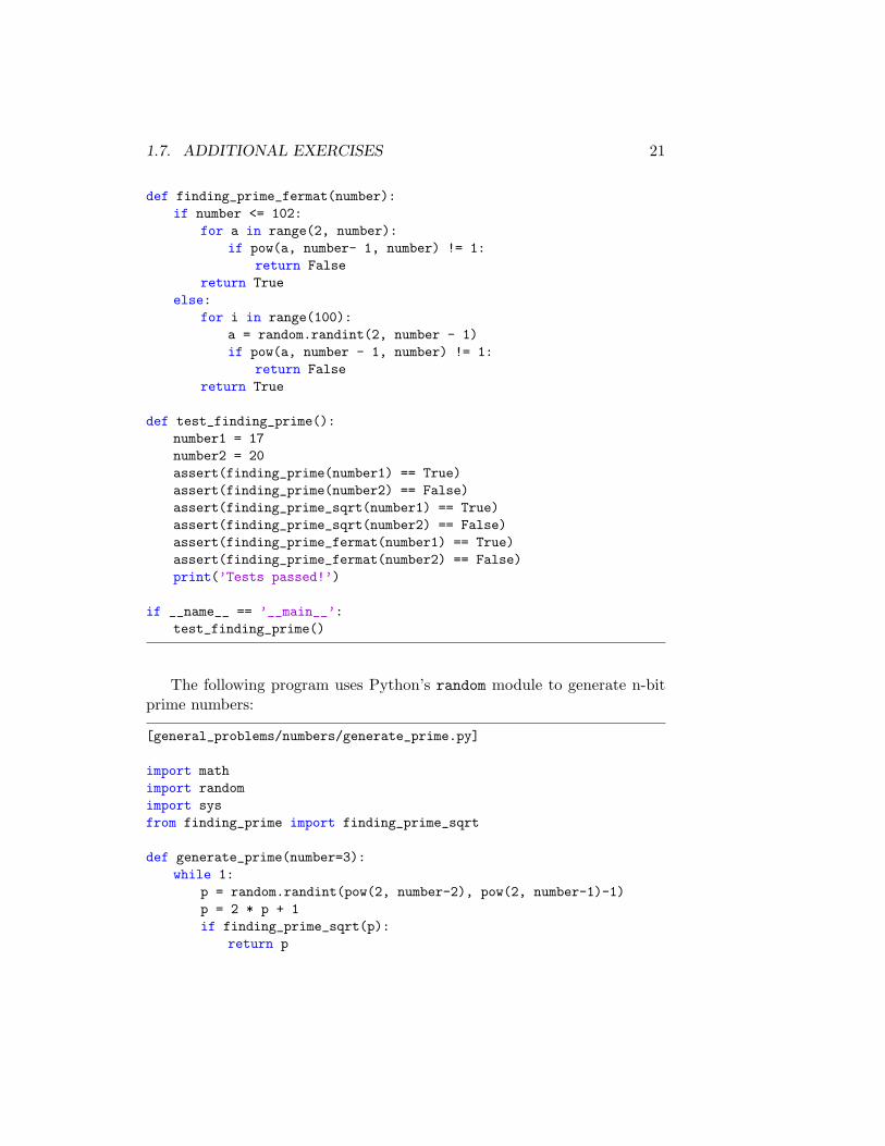
The following program uses Python’s random module to generate n-bitprime numbers:
[general_problems/numbers/generate_prime.py]
import mathimport randomimport sysfrom finding_prime import finding_prime_sqrt
def generate_prime(number=3):while 1:
p = random.randint(pow(2, number-2), pow(2, number-1)-1)p = 2 * p + 1if finding_prime_sqrt(p):
return p
22 CHAPTER 1. NUMBERS
if __name__ == ’__main__’:if len(sys.argv) < 2:
print ("Usage: generate_prime.py number")sys.exit()
else:number = int(sys.argv[1])print(generate_prime(number))
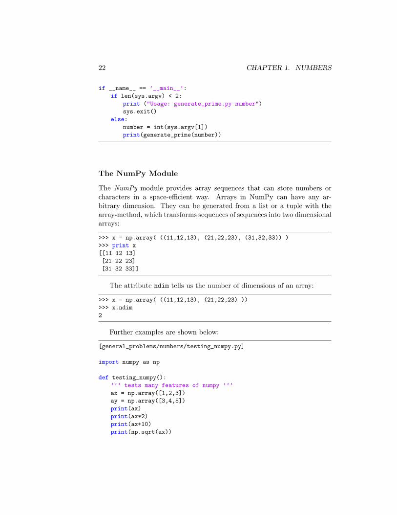
The NumPy Module
The NumPy module provides array sequences that can store numbers orcharacters in a space-efficient way. Arrays in NumPy can have any ar-bitrary dimension. They can be generated from a list or a tuple with thearray-method, which transforms sequences of sequences into two dimensionalarrays:
>>> x = np.array( ((11,12,13), (21,22,23), (31,32,33)) )>>> print x[[11 12 13][21 22 23][31 32 33]]
The attribute ndim tells us the number of dimensions of an array:
>>> x = np.array( ((11,12,13), (21,22,23) ))>>> x.ndim2
Further examples are shown below:
[general_problems/numbers/testing_numpy.py]
import numpy as np
def testing_numpy():’’’ tests many features of numpy ’’’ax = np.array([1,2,3])ay = np.array([3,4,5])print(ax)print(ax*2)print(ax+10)print(np.sqrt(ax))
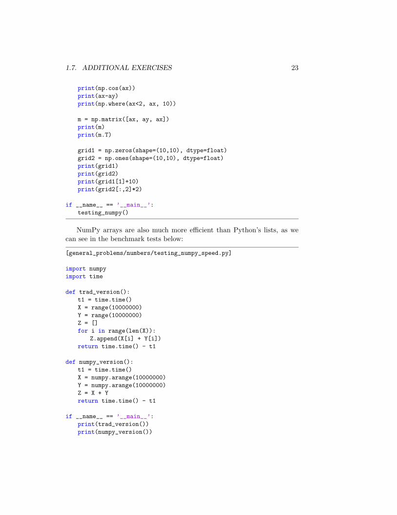
1.7. ADDITIONAL EXERCISES 23
print(np.cos(ax))print(ax-ay)print(np.where(ax<2, ax, 10))
m = np.matrix([ax, ay, ax])print(m)print(m.T)
grid1 = np.zeros(shape=(10,10), dtype=float)grid2 = np.ones(shape=(10,10), dtype=float)print(grid1)print(grid2)print(grid1[1]+10)print(grid2[:,2]*2)
if __name__ == ’__main__’:testing_numpy()
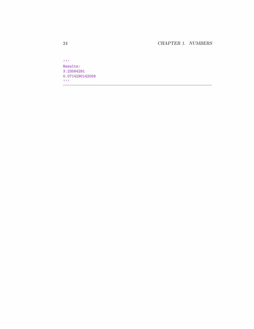
NumPy arrays are also much more efficient than Python’s lists, as wecan see in the benchmark tests below:
[general_problems/numbers/testing_numpy_speed.py]
import numpyimport time
def trad_version():t1 = time.time()X = range(10000000)Y = range(10000000)Z = []for i in range(len(X)):
Z.append(X[i] + Y[i])return time.time() - t1
def numpy_version():t1 = time.time()X = numpy.arange(10000000)Y = numpy.arange(10000000)Z = X + Yreturn time.time() - t1
if __name__ == ’__main__’:print(trad_version())print(numpy_version())
24 CHAPTER 1. NUMBERS
’’’Results:3.235642910.0714290142059’’’
Chapter 2
Built-in Sequence Types
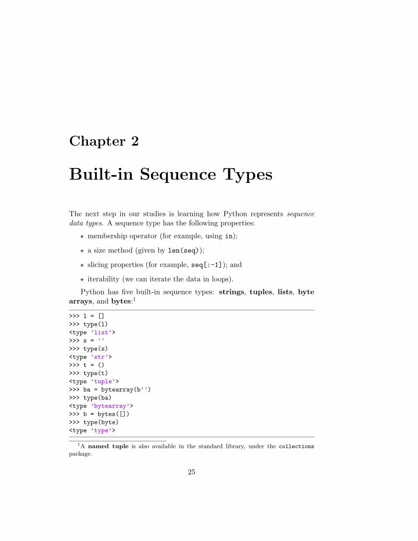
The next step in our studies is learning how Python represents sequencedata types. A sequence type has the following properties:
? membership operator (for example, using in);
? a size method (given by len(seq));
? slicing properties (for example, seq[:-1]); and
? iterability (we can iterate the data in loops).
Python has five built-in sequence types: strings, tuples, lists, bytearrays, and bytes:1
>>> l = []>>> type(l)<type ’list’>>>> s = ’’>>> type(s)<type ’str’>>>> t = ()>>> type(t)<type ’tuple’>>>> ba = bytearray(b’’)>>> type(ba)<type ’bytearray’>>>> b = bytes([])>>> type(byte)<type ’type’>
1A named tuple is also available in the standard library, under the collections
package.
25
26 CHAPTER 2. BUILT-IN SEQUENCE TYPES
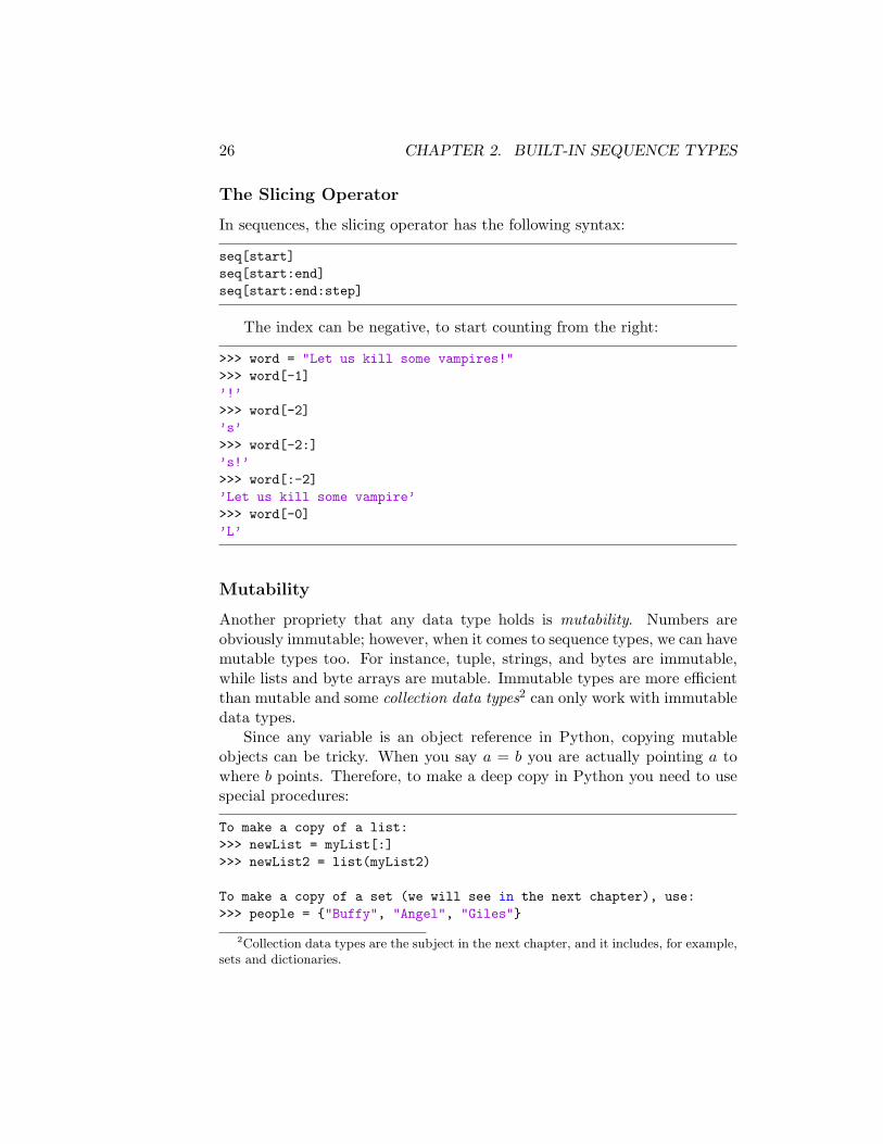
The Slicing Operator
In sequences, the slicing operator has the following syntax:
seq[start]seq[start:end]seq[start:end:step]
The index can be negative, to start counting from the right:
>>> word = "Let us kill some vampires!">>> word[-1]’!’>>> word[-2]’s’>>> word[-2:]’s!’>>> word[:-2]’Let us kill some vampire’>>> word[-0]’L’
Mutability
Another propriety that any data type holds is mutability. Numbers areobviously immutable; however, when it comes to sequence types, we can havemutable types too. For instance, tuple, strings, and bytes are immutable,while lists and byte arrays are mutable. Immutable types are more efficientthan mutable and some collection data types2 can only work with immutabledata types.
Since any variable is an object reference in Python, copying mutableobjects can be tricky. When you say a = b you are actually pointing a towhere b points. Therefore, to make a deep copy in Python you need to usespecial procedures:
To make a copy of a list:>>> newList = myList[:]>>> newList2 = list(myList2)
To make a copy of a set (we will see in the next chapter), use:>>> people = {"Buffy", "Angel", "Giles"}
2Collection data types are the subject in the next chapter, and it includes, for example,sets and dictionaries.
2.1. STRINGS 27
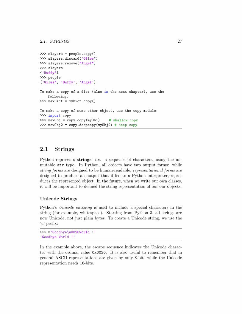
>>> slayers = people.copy()>>> slayers.discard("Giles")>>> slayers.remove("Angel")>>> slayers{’Buffy’}>>> people{’Giles’, ’Buffy’, ’Angel’}
To make a copy of a dict (also in the next chapter), use thefollowing:
>>> newDict = myDict.copy()
To make a copy of some other object, use the copy module:>>> import copy>>> newObj = copy.copy(myObj) # shallow copy>>> newObj2 = copy.deepcopy(myObj2) # deep copy
2.1 Strings
Python represents strings, i.e. a sequence of characters, using the im-mutable str type. In Python, all objects have two output forms: whilestring forms are designed to be human-readable, representational forms aredesigned to produce an output that if fed to a Python interpreter, repro-duces the represented object. In the future, when we write our own classes,it will be important to defined the string representation of our our objects.
Unicode Strings
Python’s Unicode encoding is used to include a special characters in thestring (for example, whitespace). Starting from Python 3, all strings arenow Unicode, not just plain bytes. To create a Unicode string, we use the‘u’ prefix:
>>> u’Goodbye\u0020World !’’Goodbye World !’
In the example above, the escape sequence indicates the Unicode charac-ter with the ordinal value 0x0020. It is also useful to remember that ingeneral ASCII representations are given by only 8-bits while the Unicoderepresentation needs 16-bits.
28 CHAPTER 2. BUILT-IN SEQUENCE TYPES
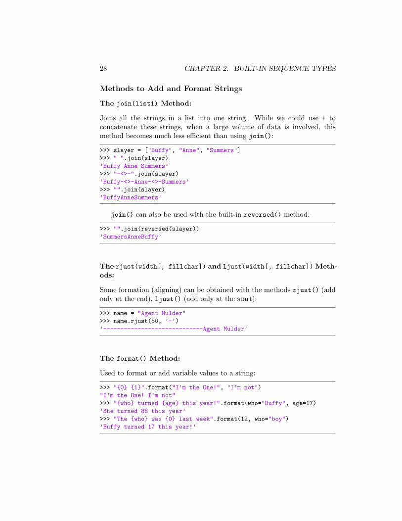
Methods to Add and Format Strings
The join(list1) Method:
Joins all the strings in a list into one string. While we could use + toconcatenate these strings, when a large volume of data is involved, thismethod becomes much less efficient than using join():
>>> slayer = ["Buffy", "Anne", "Summers"]>>> " ".join(slayer)’Buffy Anne Summers’>>> "-<>-".join(slayer)’Buffy-<>-Anne-<>-Summers’>>> "".join(slayer)’BuffyAnneSummers’
join() can also be used with the built-in reversed() method:
>>> "".join(reversed(slayer))’SummersAnneBuffy’
The rjust(width[, fillchar]) and ljust(width[, fillchar]) Meth-ods:
Some formation (aligning) can be obtained with the methods rjust() (addonly at the end), ljust() (add only at the start):
>>> name = "Agent Mulder">>> name.rjust(50, ’-’)’-----------------------------Agent Mulder’
The format() Method:
Used to format or add variable values to a string:
>>> "{0} {1}".format("I’m the One!", "I’m not")"I’m the One! I’m not">>> "{who} turned {age} this year!".format(who="Buffy", age=17)’She turned 88 this year’>>> "The {who} was {0} last week".format(12, who="boy")’Buffy turned 17 this year!’
2.1. STRINGS 29
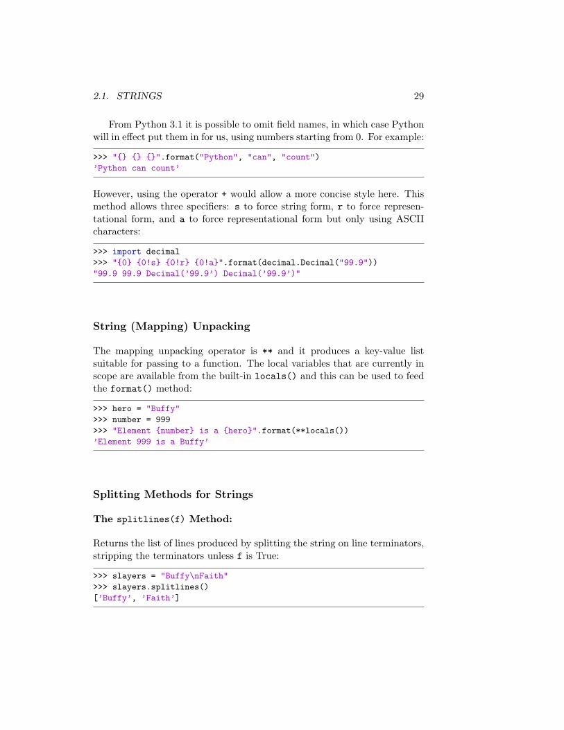
From Python 3.1 it is possible to omit field names, in which case Pythonwill in effect put them in for us, using numbers starting from 0. For example:
>>> "{} {} {}".format("Python", "can", "count")’Python can count’
However, using the operator + would allow a more concise style here. Thismethod allows three specifiers: s to force string form, r to force represen-tational form, and a to force representational form but only using ASCIIcharacters:
>>> import decimal>>> "{0} {0!s} {0!r} {0!a}".format(decimal.Decimal("99.9"))"99.9 99.9 Decimal(’99.9’) Decimal(’99.9’)"
String (Mapping) Unpacking
The mapping unpacking operator is ** and it produces a key-value listsuitable for passing to a function. The local variables that are currently inscope are available from the built-in locals() and this can be used to feedthe format() method:
>>> hero = "Buffy">>> number = 999>>> "Element {number} is a {hero}".format(**locals())’Element 999 is a Buffy’
Splitting Methods for Strings
The splitlines(f) Method:
Returns the list of lines produced by splitting the string on line terminators,stripping the terminators unless f is True:
>>> slayers = "Buffy\nFaith">>> slayers.splitlines()[’Buffy’, ’Faith’]
30 CHAPTER 2. BUILT-IN SEQUENCE TYPES
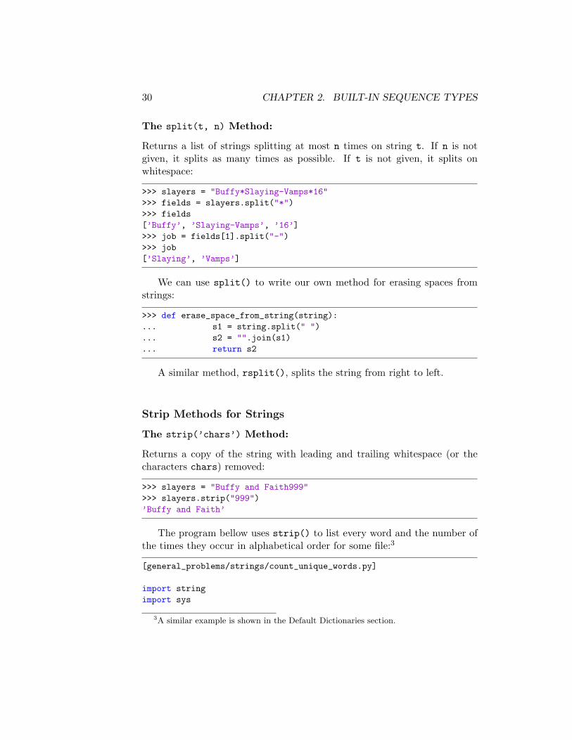
The split(t, n) Method:
Returns a list of strings splitting at most n times on string t. If n is notgiven, it splits as many times as possible. If t is not given, it splits onwhitespace:
>>> slayers = "Buffy*Slaying-Vamps*16">>> fields = slayers.split("*")>>> fields[’Buffy’, ’Slaying-Vamps’, ’16’]>>> job = fields[1].split("-")>>> job[’Slaying’, ’Vamps’]
We can use split() to write our own method for erasing spaces fromstrings:
>>> def erase_space_from_string(string):... s1 = string.split(" ")... s2 = "".join(s1)... return s2
A similar method, rsplit(), splits the string from right to left.
Strip Methods for Strings
The strip(’chars’) Method:
Returns a copy of the string with leading and trailing whitespace (or thecharacters chars) removed:
>>> slayers = "Buffy and Faith999">>> slayers.strip("999")’Buffy and Faith’
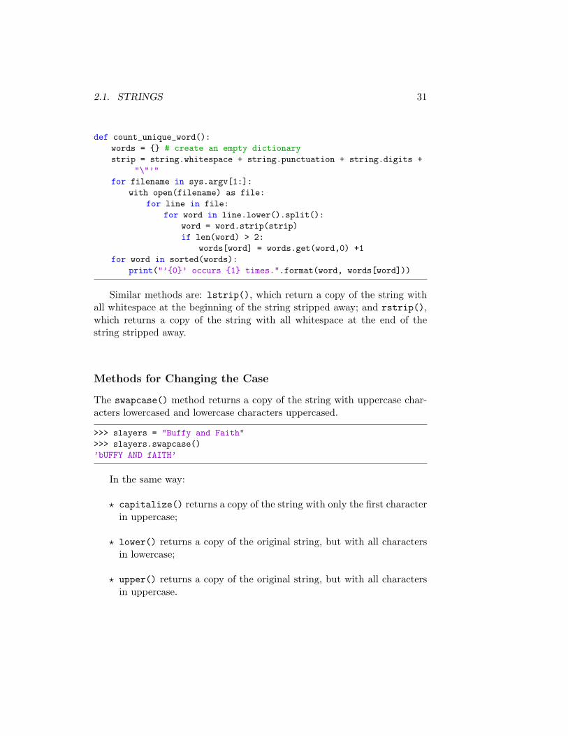
The program bellow uses strip() to list every word and the number ofthe times they occur in alphabetical order for some file:3
[general_problems/strings/count_unique_words.py]
import stringimport sys
3A similar example is shown in the Default Dictionaries section.
2.1. STRINGS 31
def count_unique_word():words = {} # create an empty dictionarystrip = string.whitespace + string.punctuation + string.digits +
"\"’"for filename in sys.argv[1:]:
with open(filename) as file:for line in file:
for word in line.lower().split():word = word.strip(strip)if len(word) > 2:
words[word] = words.get(word,0) +1for word in sorted(words):
print("’{0}’ occurs {1} times.".format(word, words[word]))
Similar methods are: lstrip(), which return a copy of the string withall whitespace at the beginning of the string stripped away; and rstrip(),which returns a copy of the string with all whitespace at the end of thestring stripped away.
Methods for Changing the Case
The swapcase() method returns a copy of the string with uppercase char-acters lowercased and lowercase characters uppercased.
>>> slayers = "Buffy and Faith">>> slayers.swapcase()’bUFFY AND fAITH’
In the same way:
? capitalize() returns a copy of the string with only the first characterin uppercase;
? lower() returns a copy of the original string, but with all charactersin lowercase;
? upper() returns a copy of the original string, but with all charactersin uppercase.
32 CHAPTER 2. BUILT-IN SEQUENCE TYPES
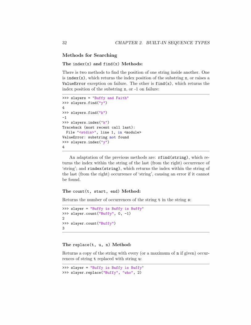
Methods for Searching
The index(x) and find(x) Methods:
There is two methods to find the position of one string inside another. Oneis index(x), which returns the index position of the substring x, or raises aValueError exception on failure. The other is find(x), which returns theindex position of the substring x, or -1 on failure:
>>> slayers = "Buffy and Faith">>> slayers.find("y")4>>> slayers.find("k")-1>>> slayers.index("k")Traceback (most recent call last):File "<stdin>", line 1, in <module>
ValueError: substring not found>>> slayers.index("y")4
An adaptation of the previous methods are: rfind(string), which re-turns the index within the string of the last (from the right) occurrence of‘string’; and rindex(string), which returns the index within the string ofthe last (from the right) occurrence of ‘string’, causing an error if it cannotbe found.
The count(t, start, end) Method:
Returns the number of occurrences of the string t in the string s:
>>> slayer = "Buffy is Buffy is Buffy">>> slayer.count("Buffy", 0, -1)2>>> slayer.count("Buffy")3
The replace(t, u, n) Method:
Returns a copy of the string with every (or a maximum of n if given) occur-rences of string t replaced with string u:
>>> slayer = "Buffy is Buffy is Buffy">>> slayer.replace("Buffy", "who", 2)
2.2. TUPLES 33
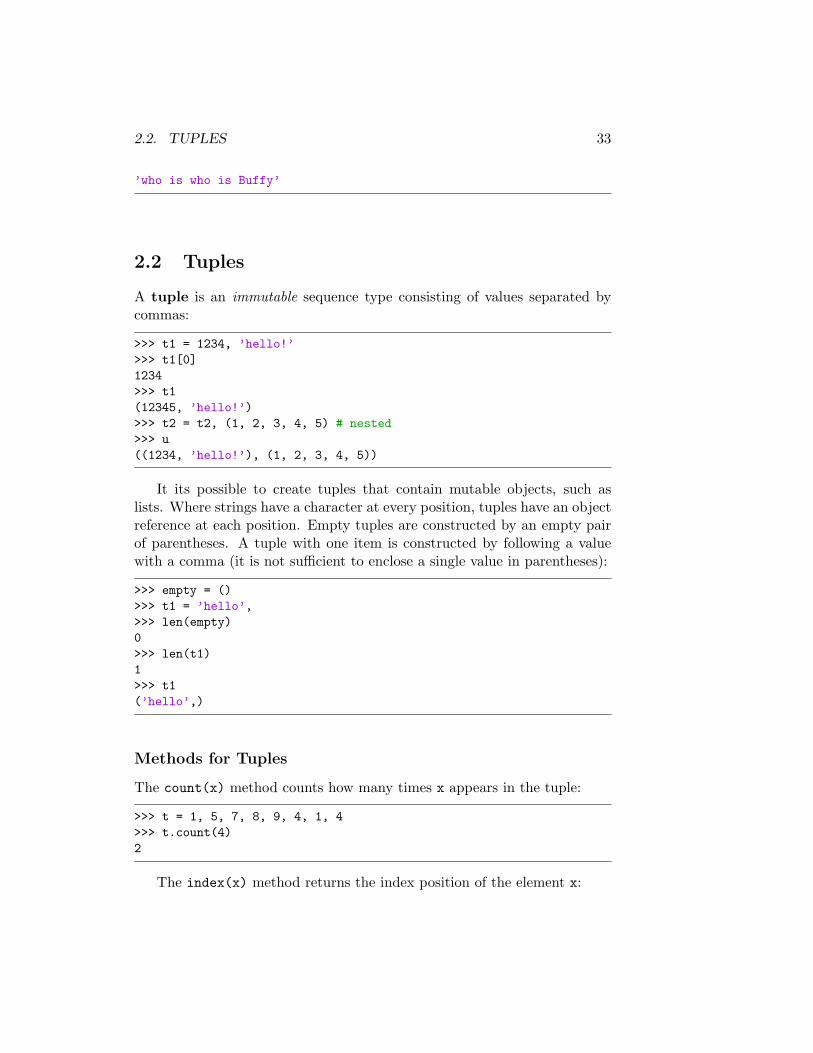
’who is who is Buffy’
2.2 Tuples
A tuple is an immutable sequence type consisting of values separated bycommas:
>>> t1 = 1234, ’hello!’>>> t1[0]1234>>> t1(12345, ’hello!’)>>> t2 = t2, (1, 2, 3, 4, 5) # nested>>> u((1234, ’hello!’), (1, 2, 3, 4, 5))
It its possible to create tuples that contain mutable objects, such aslists. Where strings have a character at every position, tuples have an objectreference at each position. Empty tuples are constructed by an empty pairof parentheses. A tuple with one item is constructed by following a valuewith a comma (it is not sufficient to enclose a single value in parentheses):
>>> empty = ()>>> t1 = ’hello’,>>> len(empty)0>>> len(t1)1>>> t1(’hello’,)
Methods for Tuples
The count(x) method counts how many times x appears in the tuple:
>>> t = 1, 5, 7, 8, 9, 4, 1, 4>>> t.count(4)2
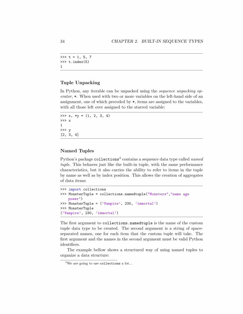
The index(x) method returns the index position of the element x:
34 CHAPTER 2. BUILT-IN SEQUENCE TYPES
>>> t = 1, 5, 7>>> t.index(5)1
Tuple Unpacking
In Python, any iterable can be unpacked using the sequence unpacking op-erator, *. When used with two or more variables on the left-hand side of anassignment, one of which preceded by *, items are assigned to the variables,with all those left over assigned to the starred variable:
>>> x, *y = (1, 2, 3, 4)>>> x1>>> y[2, 3, 4]
Named Tuples
Python’s package collections4 contains a sequence data type called namedtuple. This behaves just like the built-in tuple, with the same performancecharacteristics, but it also carries the ability to refer to items in the tupleby name as well as by index position. This allows the creation of aggregatesof data items:
>>> import collections>>> MonsterTuple = collections.namedtuple("Monsters","name age
power")>>> MonsterTuple = (’Vampire’, 230, ’immortal’)>>> MonsterTuple(’Vampire’, 230, ’immortal’)
The first argument to collections.namedtuple is the name of the customtuple data type to be created. The second argument is a string of space-separated names, one for each item that the custom tuple will take. Thefirst argument and the names in the second argument must be valid Pythonidentifiers.
The example bellow shows a structured way of using named tuples toorganize a data structure:
4We are going to use collections a lot...
2.3. LISTS 35
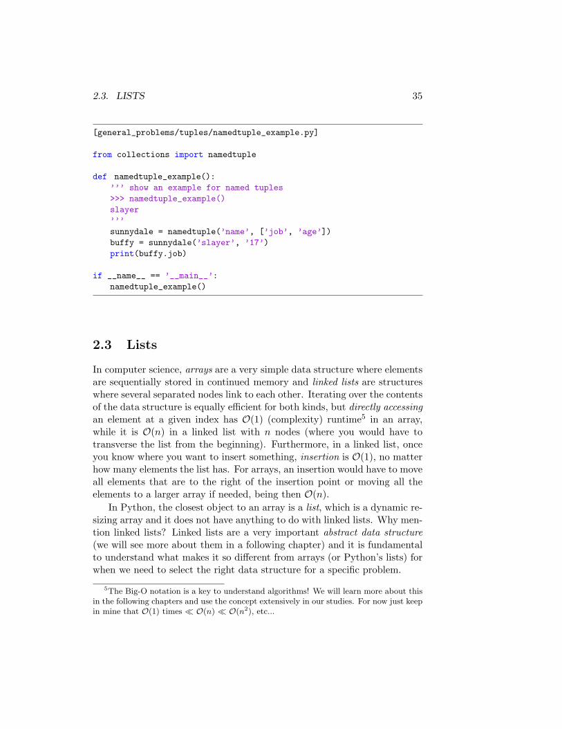
[general_problems/tuples/namedtuple_example.py]
from collections import namedtuple
def namedtuple_example():’’’ show an example for named tuples>>> namedtuple_example()slayer’’’sunnydale = namedtuple(’name’, [’job’, ’age’])buffy = sunnydale(’slayer’, ’17’)print(buffy.job)
if __name__ == ’__main__’:namedtuple_example()
2.3 Lists
In computer science, arrays are a very simple data structure where elementsare sequentially stored in continued memory and linked lists are structureswhere several separated nodes link to each other. Iterating over the contentsof the data structure is equally efficient for both kinds, but directly accessingan element at a given index has O(1) (complexity) runtime5 in an array,while it is O(n) in a linked list with n nodes (where you would have totransverse the list from the beginning). Furthermore, in a linked list, onceyou know where you want to insert something, insertion is O(1), no matterhow many elements the list has. For arrays, an insertion would have to moveall elements that are to the right of the insertion point or moving all theelements to a larger array if needed, being then O(n).
In Python, the closest object to an array is a list, which is a dynamic re-sizing array and it does not have anything to do with linked lists. Why men-tion linked lists? Linked lists are a very important abstract data structure(we will see more about them in a following chapter) and it is fundamentalto understand what makes it so different from arrays (or Python’s lists) forwhen we need to select the right data structure for a specific problem.
5The Big-O notation is a key to understand algorithms! We will learn more about thisin the following chapters and use the concept extensively in our studies. For now just keepin mine that O(1) times � O(n) � O(n2), etc...
36 CHAPTER 2. BUILT-IN SEQUENCE TYPES
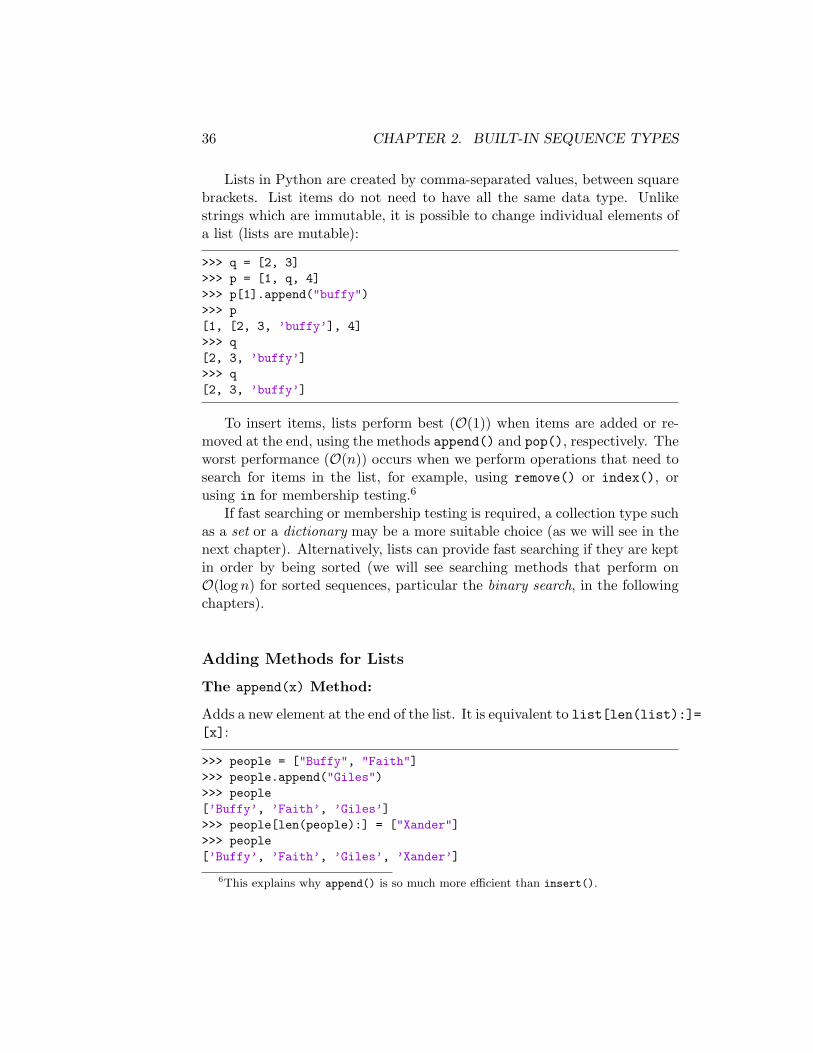
Lists in Python are created by comma-separated values, between squarebrackets. List items do not need to have all the same data type. Unlikestrings which are immutable, it is possible to change individual elements ofa list (lists are mutable):
>>> q = [2, 3]>>> p = [1, q, 4]>>> p[1].append("buffy")>>> p[1, [2, 3, ’buffy’], 4]>>> q[2, 3, ’buffy’]>>> q[2, 3, ’buffy’]
To insert items, lists perform best (O(1)) when items are added or re-moved at the end, using the methods append() and pop(), respectively. Theworst performance (O(n)) occurs when we perform operations that need tosearch for items in the list, for example, using remove() or index(), orusing in for membership testing.6
If fast searching or membership testing is required, a collection type suchas a set or a dictionary may be a more suitable choice (as we will see in thenext chapter). Alternatively, lists can provide fast searching if they are keptin order by being sorted (we will see searching methods that perform onO(log n) for sorted sequences, particular the binary search, in the followingchapters).
Adding Methods for Lists
The append(x) Method:
Adds a new element at the end of the list. It is equivalent to list[len(list):]=[x]:
>>> people = ["Buffy", "Faith"]>>> people.append("Giles")>>> people[’Buffy’, ’Faith’, ’Giles’]>>> people[len(people):] = ["Xander"]>>> people[’Buffy’, ’Faith’, ’Giles’, ’Xander’]
6This explains why append() is so much more efficient than insert().
2.3. LISTS 37
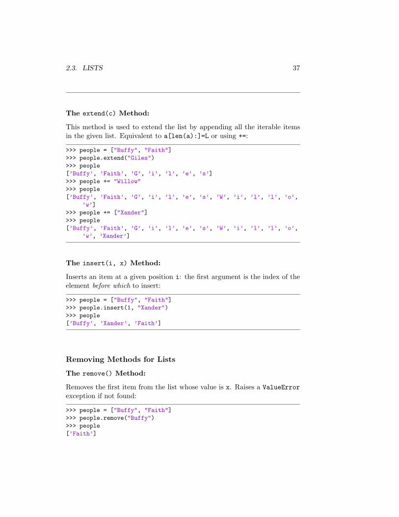
The extend(c) Method:
This method is used to extend the list by appending all the iterable itemsin the given list. Equivalent to a[len(a):]=L or using +=:
>>> people = ["Buffy", "Faith"]>>> people.extend("Giles")>>> people[’Buffy’, ’Faith’, ’G’, ’i’, ’l’, ’e’, ’s’]>>> people += "Willow">>> people[’Buffy’, ’Faith’, ’G’, ’i’, ’l’, ’e’, ’s’, ’W’, ’i’, ’l’, ’l’, ’o’,
’w’]>>> people += ["Xander"]>>> people[’Buffy’, ’Faith’, ’G’, ’i’, ’l’, ’e’, ’s’, ’W’, ’i’, ’l’, ’l’, ’o’,
’w’, ’Xander’]
The insert(i, x) Method:
Inserts an item at a given position i: the first argument is the index of theelement before which to insert:
>>> people = ["Buffy", "Faith"]>>> people.insert(1, "Xander")>>> people[’Buffy’, ’Xander’, ’Faith’]
Removing Methods for Lists
The remove() Method:
Removes the first item from the list whose value is x. Raises a ValueErrorexception if not found:
>>> people = ["Buffy", "Faith"]>>> people.remove("Buffy")>>> people[’Faith’]
38 CHAPTER 2. BUILT-IN SEQUENCE TYPES
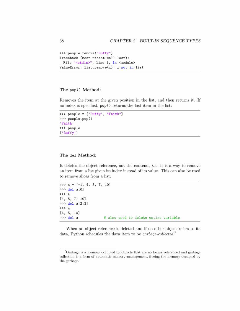
>>> people.remove("Buffy")Traceback (most recent call last):File "<stdin>", line 1, in <module>
ValueError: list.remove(x): x not in list
The pop() Method:
Removes the item at the given position in the list, and then returns it. Ifno index is specified, pop() returns the last item in the list:
>>> people = ["Buffy", "Faith"]>>> people.pop()’Faith’>>> people[’Buffy’]
The del Method:
It deletes the object reference, not the contend, i.e., it is a way to removean item from a list given its index instead of its value. This can also be usedto remove slices from a list:
>>> a = [-1, 4, 5, 7, 10]>>> del a[0]>>> a[4, 5, 7, 10]>>> del a[2:3]>>> a[4, 5, 10]>>> del a # also used to delete entire variable
When an object reference is deleted and if no other object refers to itsdata, Python schedules the data item to be garbage-collected.7
7Garbage is a memory occupied by objects that are no longer referenced and garbagecollection is a form of automatic memory management, freeing the memory occupied bythe garbage.
2.3. LISTS 39
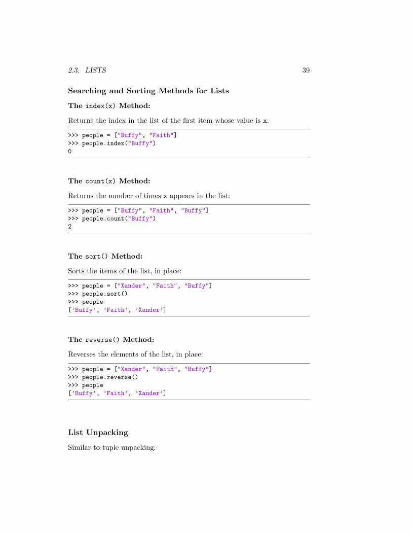
Searching and Sorting Methods for Lists
The index(x) Method:
Returns the index in the list of the first item whose value is x:
>>> people = ["Buffy", "Faith"]>>> people.index("Buffy")0
The count(x) Method:
Returns the number of times x appears in the list:
>>> people = ["Buffy", "Faith", "Buffy"]>>> people.count("Buffy")2
The sort() Method:
Sorts the items of the list, in place:
>>> people = ["Xander", "Faith", "Buffy"]>>> people.sort()>>> people[’Buffy’, ’Faith’, ’Xander’]
The reverse() Method:
Reverses the elements of the list, in place:
>>> people = ["Xander", "Faith", "Buffy"]>>> people.reverse()>>> people[’Buffy’, ’Faith’, ’Xander’]
List Unpacking
Similar to tuple unpacking:
40 CHAPTER 2. BUILT-IN SEQUENCE TYPES
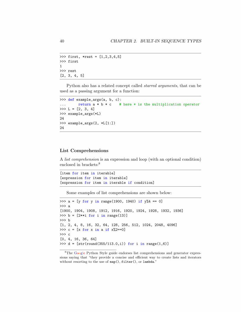
>>> first, *rest = [1,2,3,4,5]>>> first1>>> rest[2, 3, 4, 5]
Python also has a related concept called starred arguments, that can beused as a passing argument for a function:
>>> def example_args(a, b, c):... return a * b * c # here * is the multiplication operator>>> L = [2, 3, 4]>>> example_args(*L)24>>> example_args(2, *L[1:])24
List Comprehensions
A list comprehension is an expression and loop (with an optional condition)enclosed in brackets:8
[item for item in iterable][expression for item in iterable][expression for item in iterable if condition]
Some examples of list comprehensions are shown below:
>>> a = [y for y in range(1900, 1940) if y%4 == 0]>>> a[1900, 1904, 1908, 1912, 1916, 1920, 1924, 1928, 1932, 1936]>>> b = [2**i for i in range(13)]>>> b[1, 2, 4, 8, 16, 32, 64, 128, 256, 512, 1024, 2048, 4096]>>> c = [x for x in a if x%2==0]>>> c[0, 4, 16, 36, 64]>>> d = [str(round(355/113.0,i)) for i in range(1,6)]
8The Google Python Style guide endorses list comprehensions and generator expres-sions saying that “they provide a concise and efficient way to create lists and iteratorswithout resorting to the use of map(), filter(), or lambda.”
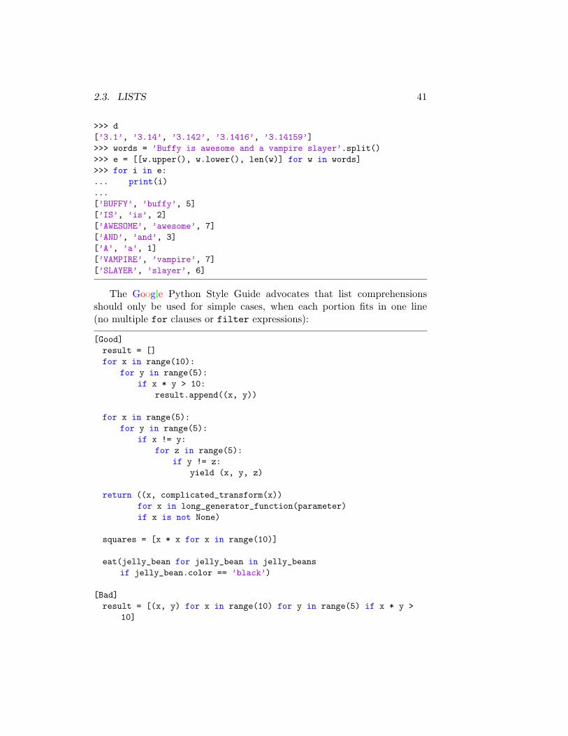
2.3. LISTS 41
>>> d[’3.1’, ’3.14’, ’3.142’, ’3.1416’, ’3.14159’]>>> words = ’Buffy is awesome and a vampire slayer’.split()>>> e = [[w.upper(), w.lower(), len(w)] for w in words]>>> for i in e:... print(i)...[’BUFFY’, ’buffy’, 5][’IS’, ’is’, 2][’AWESOME’, ’awesome’, 7][’AND’, ’and’, 3][’A’, ’a’, 1][’VAMPIRE’, ’vampire’, 7][’SLAYER’, ’slayer’, 6]
The Google Python Style Guide advocates that list comprehensionsshould only be used for simple cases, when each portion fits in one line(no multiple for clauses or filter expressions):
[Good]result = []for x in range(10):
for y in range(5):if x * y > 10:
result.append((x, y))
for x in range(5):for y in range(5):
if x != y:for z in range(5):
if y != z:yield (x, y, z)
return ((x, complicated_transform(x))for x in long_generator_function(parameter)if x is not None)
squares = [x * x for x in range(10)]
eat(jelly_bean for jelly_bean in jelly_beansif jelly_bean.color == ’black’)
[Bad]result = [(x, y) for x in range(10) for y in range(5) if x * y >
10]
42 CHAPTER 2. BUILT-IN SEQUENCE TYPES
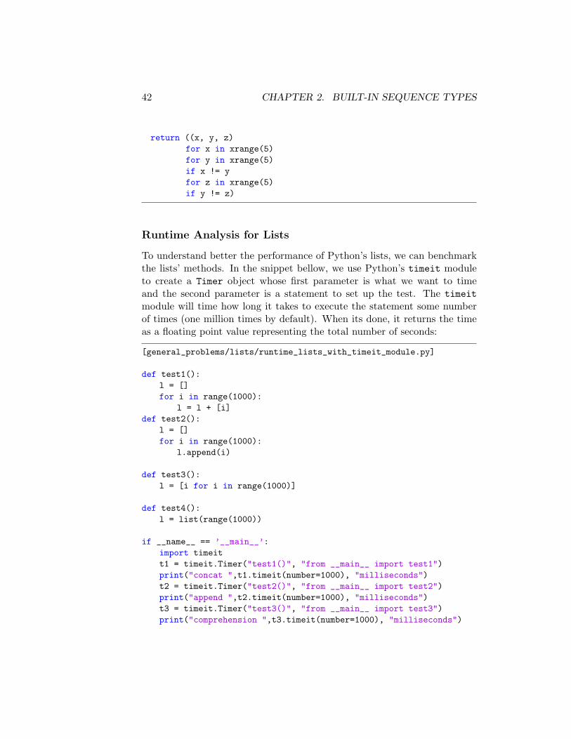
return ((x, y, z)for x in xrange(5)for y in xrange(5)if x != yfor z in xrange(5)if y != z)
Runtime Analysis for Lists
To understand better the performance of Python’s lists, we can benchmarkthe lists’ methods. In the snippet bellow, we use Python’s timeit moduleto create a Timer object whose first parameter is what we want to timeand the second parameter is a statement to set up the test. The timeitmodule will time how long it takes to execute the statement some numberof times (one million times by default). When its done, it returns the timeas a floating point value representing the total number of seconds:
[general_problems/lists/runtime_lists_with_timeit_module.py]
def test1():l = []for i in range(1000):
l = l + [i]def test2():
l = []for i in range(1000):
l.append(i)
def test3():l = [i for i in range(1000)]
def test4():l = list(range(1000))
if __name__ == ’__main__’:import timeitt1 = timeit.Timer("test1()", "from __main__ import test1")print("concat ",t1.timeit(number=1000), "milliseconds")t2 = timeit.Timer("test2()", "from __main__ import test2")print("append ",t2.timeit(number=1000), "milliseconds")t3 = timeit.Timer("test3()", "from __main__ import test3")print("comprehension ",t3.timeit(number=1000), "milliseconds")
2.4. BYTES AND BYTE ARRAYS 43
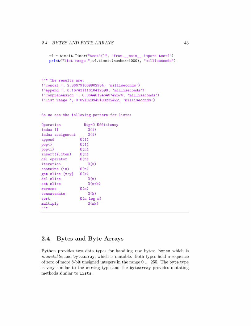
t4 = timeit.Timer("test4()", "from __main__ import test4")print("list range ",t4.timeit(number=1000), "milliseconds")
""" The results are:(’concat ’, 2.366791009902954, ’milliseconds’)(’append ’, 0.16743111610412598, ’milliseconds’)(’comprehension ’, 0.06446194648742676, ’milliseconds’)(’list range ’, 0.021029949188232422, ’milliseconds’)
So we see the following pattern for lists:
Operation Big-O Efficiencyindex [] O(1)index assignment O(1)append O(1)pop() O(1)pop(i) O(n)insert(i,item) O(n)del operator O(n)iteration O(n)contains (in) O(n)get slice [x:y] O(k)del slice O(n)set slice O(n+k)reverse O(n)concatenate O(k)sort O(n log n)multiply O(nk)"""
2.4 Bytes and Byte Arrays
Python provides two data types for handling raw bytes: bytes which isimmutable, and bytearray, which is mutable. Both types hold a sequenceof zero of more 8-bit unsigned integers in the range 0 ... 255. The byte typeis very similar to the string type and the bytearray provides mutatingmethods similar to lists.
44 CHAPTER 2. BUILT-IN SEQUENCE TYPES
Bits and Bitwise Operations
Bitwise operations can be very useful to manipulate numbers represented asbits (for example, reproduce an division without using the division opera-tion). We can you quickly compute 2x by the left-shifting operation: 1� x.We can also quickly verify whether a number is a power of 2 by checkingwhether x&(x− 1) is 0 (if x is not an even power of 2, the highest positionof x with a 1 will also have a 1 in x − 1, otherwise, x will be 100...0 andx− 1 will be 011...1; add them together they will return 0).
Chapter 3
Collection Data Structures
Differently from the last chapter’s sequence data structures, where the datacan be ordered or sliced, collection data structures are containers whichaggregates data without relating them. Collection data structures also havesome proprieties that sequence types have:
? membership operator (for example, using in);
? a size method (given by len(seq)); and
? iterability (we can iterate the data in loops).
In Python, built-in collection data types are given by sets and dicts. Inaddition, many useful collection data are found in the package collections,as we will discuss in the last part of this chapter.
3.1 Sets
In Python, a Set is an unordered collection data type that is iterable, mu-table, and has no duplicate elements. Sets are used for membership testingand eliminating duplicate entries. Sets have O(1) insertion, so the runtimeof union is O(m+n). For intersection, it is only necessary to transverse thesmaller set, so the runtime is O(n). 1
1Python’s collection package has supporting for Ordered sets. This data type enforcessome predefined comparison for their members.
45
46 CHAPTER 3. COLLECTION DATA STRUCTURES
Frozen Sets
Frozen sets are immutable objects that only support methods and opera-tors that produce a result without affecting the frozen set or sets to whichthey are applied.
Adding Methods for Sets
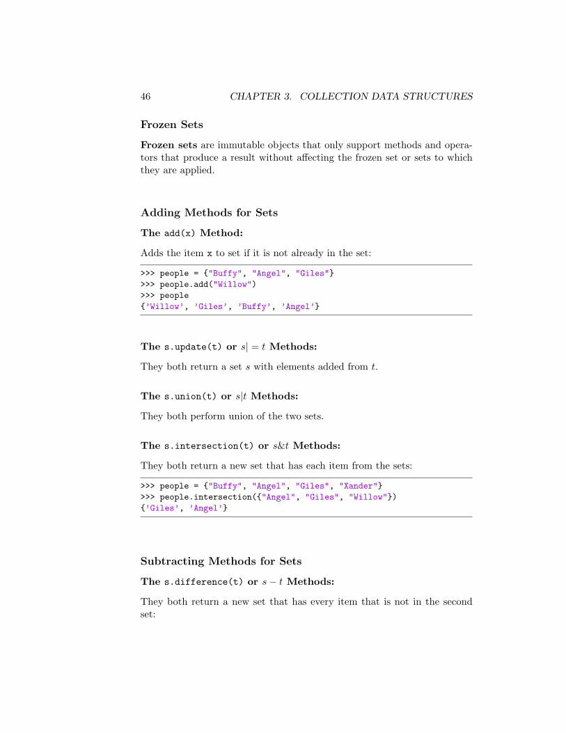
The add(x) Method:
Adds the item x to set if it is not already in the set:
>>> people = {"Buffy", "Angel", "Giles"}>>> people.add("Willow")>>> people{’Willow’, ’Giles’, ’Buffy’, ’Angel’}
The s.update(t) or s| = t Methods:
They both return a set s with elements added from t.
The s.union(t) or s|t Methods:
They both perform union of the two sets.
The s.intersection(t) or s&t Methods:
They both return a new set that has each item from the sets:
>>> people = {"Buffy", "Angel", "Giles", "Xander"}>>> people.intersection({"Angel", "Giles", "Willow"}){’Giles’, ’Angel’}
Subtracting Methods for Sets
The s.difference(t) or s− t Methods:
They both return a new set that has every item that is not in the secondset:
3.1. SETS 47
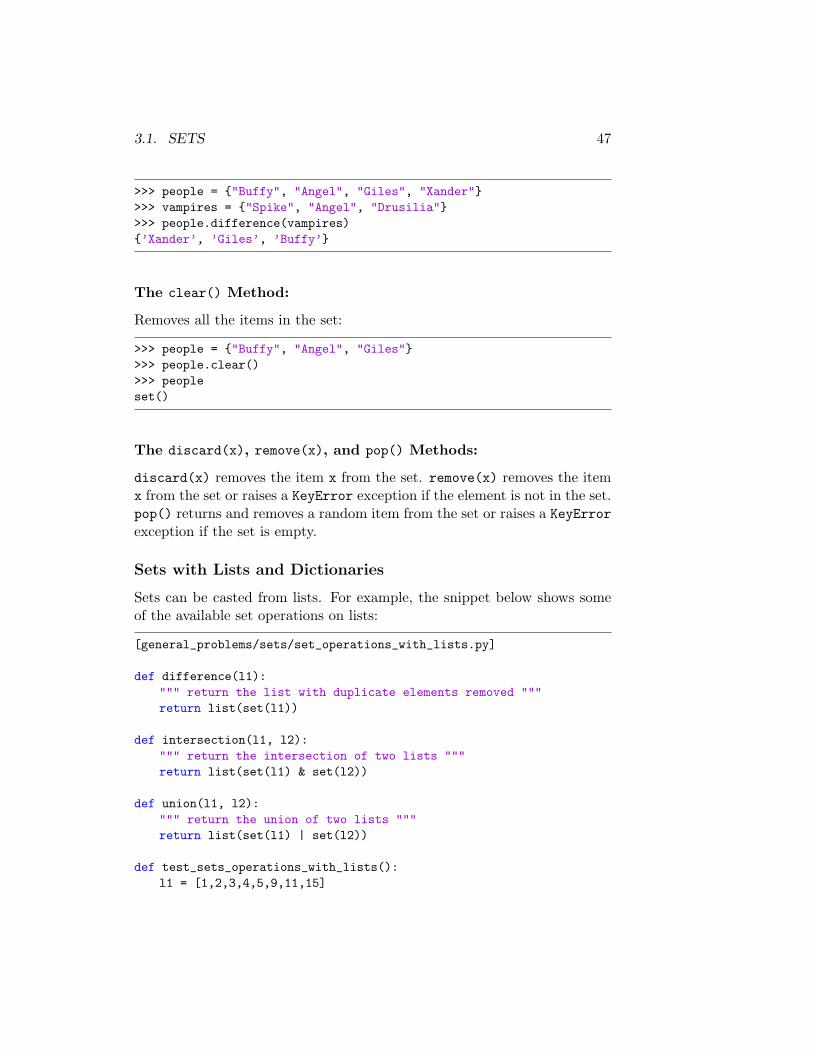
>>> people = {"Buffy", "Angel", "Giles", "Xander"}>>> vampires = {"Spike", "Angel", "Drusilia"}>>> people.difference(vampires){’Xander’, ’Giles’, ’Buffy’}
The clear() Method:
Removes all the items in the set:
>>> people = {"Buffy", "Angel", "Giles"}>>> people.clear()>>> peopleset()
The discard(x), remove(x), and pop() Methods:
discard(x) removes the item x from the set. remove(x) removes the itemx from the set or raises a KeyError exception if the element is not in the set.pop() returns and removes a random item from the set or raises a KeyErrorexception if the set is empty.
Sets with Lists and Dictionaries
Sets can be casted from lists. For example, the snippet below shows someof the available set operations on lists:
[general_problems/sets/set_operations_with_lists.py]
def difference(l1):""" return the list with duplicate elements removed """return list(set(l1))
def intersection(l1, l2):""" return the intersection of two lists """return list(set(l1) & set(l2))
def union(l1, l2):""" return the union of two lists """return list(set(l1) | set(l2))
def test_sets_operations_with_lists():l1 = [1,2,3,4,5,9,11,15]
48 CHAPTER 3. COLLECTION DATA STRUCTURES
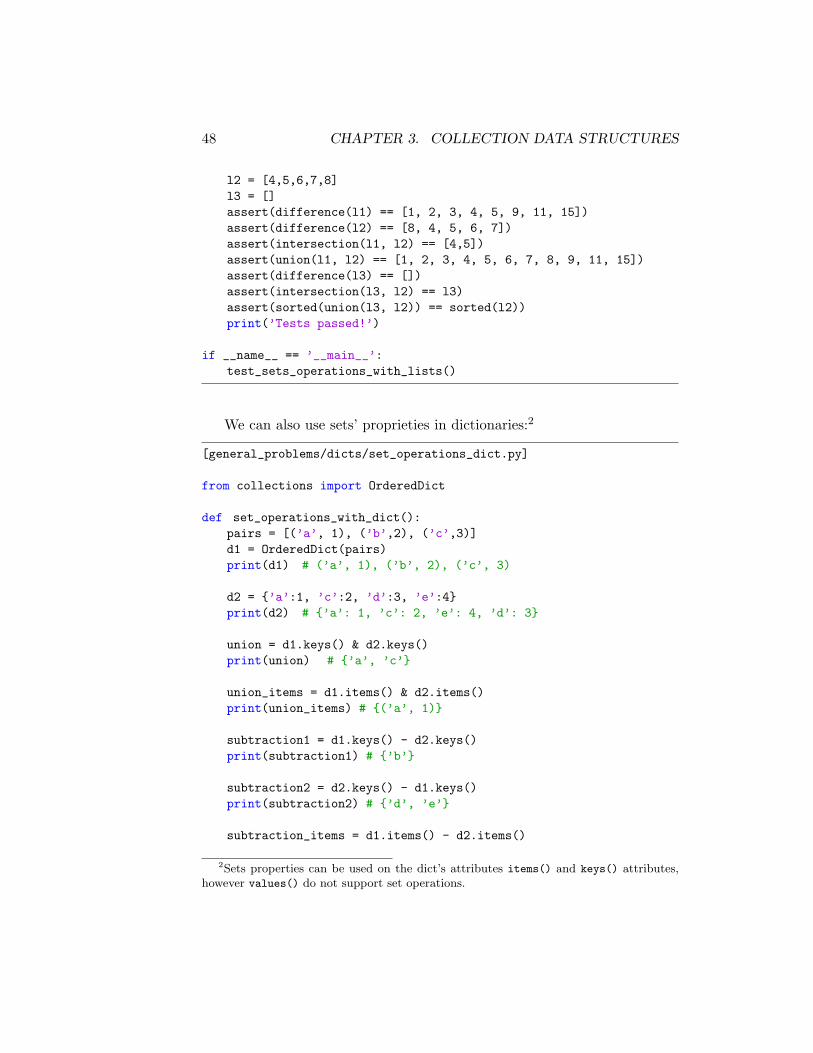
l2 = [4,5,6,7,8]l3 = []assert(difference(l1) == [1, 2, 3, 4, 5, 9, 11, 15])assert(difference(l2) == [8, 4, 5, 6, 7])assert(intersection(l1, l2) == [4,5])assert(union(l1, l2) == [1, 2, 3, 4, 5, 6, 7, 8, 9, 11, 15])assert(difference(l3) == [])assert(intersection(l3, l2) == l3)assert(sorted(union(l3, l2)) == sorted(l2))print(’Tests passed!’)
if __name__ == ’__main__’:test_sets_operations_with_lists()
We can also use sets’ proprieties in dictionaries:2
[general_problems/dicts/set_operations_dict.py]
from collections import OrderedDict
def set_operations_with_dict():pairs = [(’a’, 1), (’b’,2), (’c’,3)]d1 = OrderedDict(pairs)print(d1) # (’a’, 1), (’b’, 2), (’c’, 3)
d2 = {’a’:1, ’c’:2, ’d’:3, ’e’:4}print(d2) # {’a’: 1, ’c’: 2, ’e’: 4, ’d’: 3}
union = d1.keys() & d2.keys()print(union) # {’a’, ’c’}
union_items = d1.items() & d2.items()print(union_items) # {(’a’, 1)}
subtraction1 = d1.keys() - d2.keys()print(subtraction1) # {’b’}
subtraction2 = d2.keys() - d1.keys()print(subtraction2) # {’d’, ’e’}
subtraction_items = d1.items() - d2.items()
2Sets properties can be used on the dict’s attributes items() and keys() attributes,however values() do not support set operations.
3.2. DICTIONARIES 49
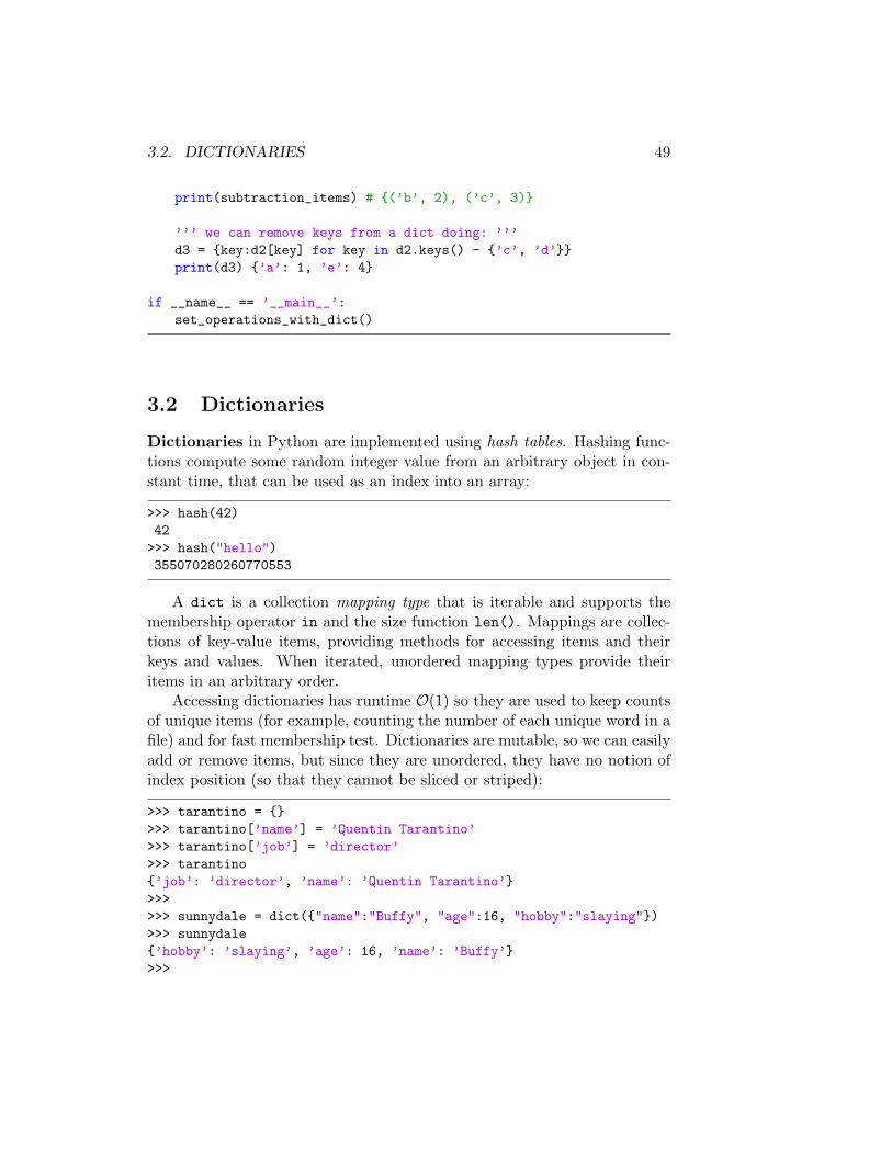
print(subtraction_items) # {(’b’, 2), (’c’, 3)}
’’’ we can remove keys from a dict doing: ’’’d3 = {key:d2[key] for key in d2.keys() - {’c’, ’d’}}print(d3) {’a’: 1, ’e’: 4}
if __name__ == ’__main__’:set_operations_with_dict()
3.2 Dictionaries
Dictionaries in Python are implemented using hash tables. Hashing func-tions compute some random integer value from an arbitrary object in con-stant time, that can be used as an index into an array:
>>> hash(42)42>>> hash("hello")355070280260770553
A dict is a collection mapping type that is iterable and supports themembership operator in and the size function len(). Mappings are collec-tions of key-value items, providing methods for accessing items and theirkeys and values. When iterated, unordered mapping types provide theiritems in an arbitrary order.
Accessing dictionaries has runtime O(1) so they are used to keep countsof unique items (for example, counting the number of each unique word in afile) and for fast membership test. Dictionaries are mutable, so we can easilyadd or remove items, but since they are unordered, they have no notion ofindex position (so that they cannot be sliced or striped):
>>> tarantino = {}>>> tarantino[’name’] = ’Quentin Tarantino’>>> tarantino[’job’] = ’director’>>> tarantino{’job’: ’director’, ’name’: ’Quentin Tarantino’}>>>>>> sunnydale = dict({"name":"Buffy", "age":16, "hobby":"slaying"})>>> sunnydale{’hobby’: ’slaying’, ’age’: 16, ’name’: ’Buffy’}>>>
50 CHAPTER 3. COLLECTION DATA STRUCTURES
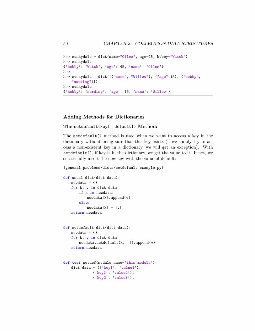
>>> sunnydale = dict(name="Giles", age=45, hobby="Watch")>>> sunnydale{’hobby’: ’Watch’, ’age’: 45, ’name’: ’Giles’}>>>>>> sunnydale = dict([("name", "Willow"), ("age",15), ("hobby",
"nerding")])>>> sunnydale{’hobby’: ’nerding’, ’age’: 15, ’name’: ’Willow’}
Adding Methods for Dictionaries
The setdefault(key[, default]) Method:
The setdefault() method is used when we want to access a key in thedictionary without being sure that this key exists (if we simply try to ac-cess a non-existent key in a dictionary, we will get an exception). Withsetdefault(), if key is in the dictionary, we get the value to it. If not, wesuccessfully insert the new key with the value of default:
[general_problems/dicts/setdefault_example.py]
def usual_dict(dict_data):newdata = {}for k, v in dict_data:
if k in newdata:newdata[k].append(v)
else:newdata[k] = [v]
return newdata
def setdefault_dict(dict_data):newdata = {}for k, v in dict_data:
newdata.setdefault(k, []).append(v)return newdata
def test_setdef(module_name=’this module’):dict_data = ((’key1’, ’value1’),
(’key1’, ’value2’),(’key2’, ’value3’),
3.2. DICTIONARIES 51
(’key2’, ’value4’),(’key2’, ’value5’),)
print(usual_dict(dict_data))print(setdefault_dict(dict_data))
s = ’Tests in {name} have {con}!’print(s.format(name=module_name, con=’passed’))
if __name__ == ’__main__’:test_setdef()
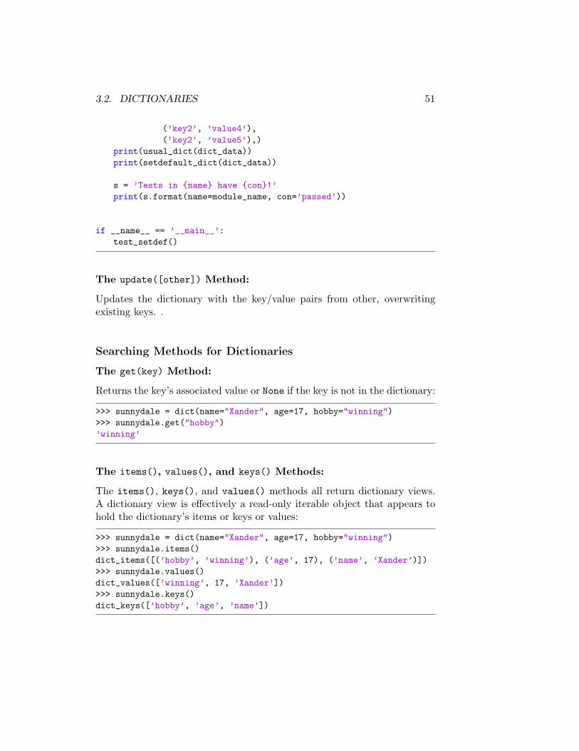
The update([other]) Method:
Updates the dictionary with the key/value pairs from other, overwritingexisting keys. .
Searching Methods for Dictionaries
The get(key) Method:
Returns the key’s associated value or None if the key is not in the dictionary:
>>> sunnydale = dict(name="Xander", age=17, hobby="winning")>>> sunnydale.get("hobby")’winning’
The items(), values(), and keys() Methods:
The items(), keys(), and values() methods all return dictionary views.A dictionary view is effectively a read-only iterable object that appears tohold the dictionary’s items or keys or values:
>>> sunnydale = dict(name="Xander", age=17, hobby="winning")>>> sunnydale.items()dict_items([(’hobby’, ’winning’), (’age’, 17), (’name’, ’Xander’)])>>> sunnydale.values()dict_values([’winning’, 17, ’Xander’])>>> sunnydale.keys()dict_keys([’hobby’, ’age’, ’name’])
52 CHAPTER 3. COLLECTION DATA STRUCTURES
Removing Methods for Dictionaries
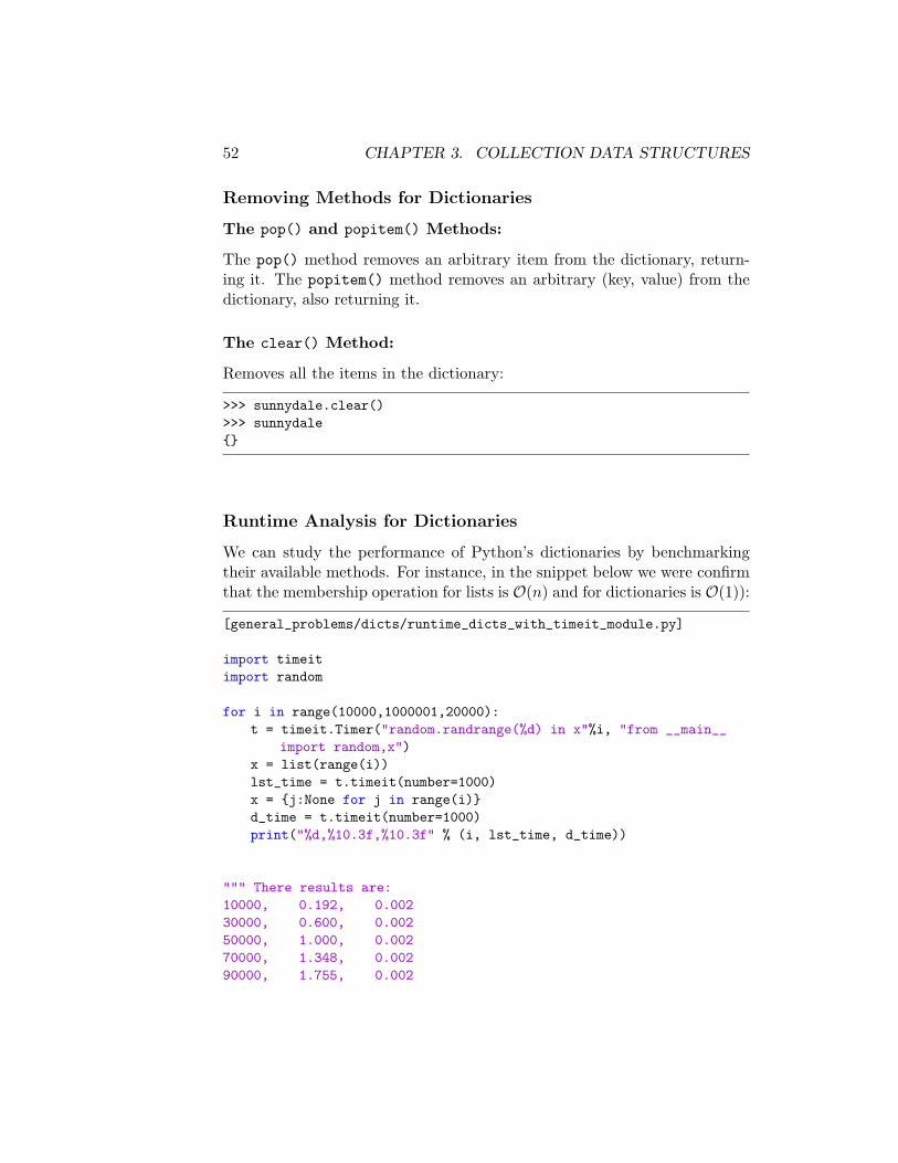
The pop() and popitem() Methods:
The pop() method removes an arbitrary item from the dictionary, return-ing it. The popitem() method removes an arbitrary (key, value) from thedictionary, also returning it.
The clear() Method:
Removes all the items in the dictionary:
>>> sunnydale.clear()>>> sunnydale{}
Runtime Analysis for Dictionaries
We can study the performance of Python’s dictionaries by benchmarkingtheir available methods. For instance, in the snippet below we were confirmthat the membership operation for lists is O(n) and for dictionaries is O(1)):
[general_problems/dicts/runtime_dicts_with_timeit_module.py]
import timeitimport random
for i in range(10000,1000001,20000):t = timeit.Timer("random.randrange(%d) in x"%i, "from __main__
import random,x")x = list(range(i))lst_time = t.timeit(number=1000)x = {j:None for j in range(i)}d_time = t.timeit(number=1000)print("%d,%10.3f,%10.3f" % (i, lst_time, d_time))
""" There results are:10000, 0.192, 0.00230000, 0.600, 0.00250000, 1.000, 0.00270000, 1.348, 0.00290000, 1.755, 0.002
3.2. DICTIONARIES 53
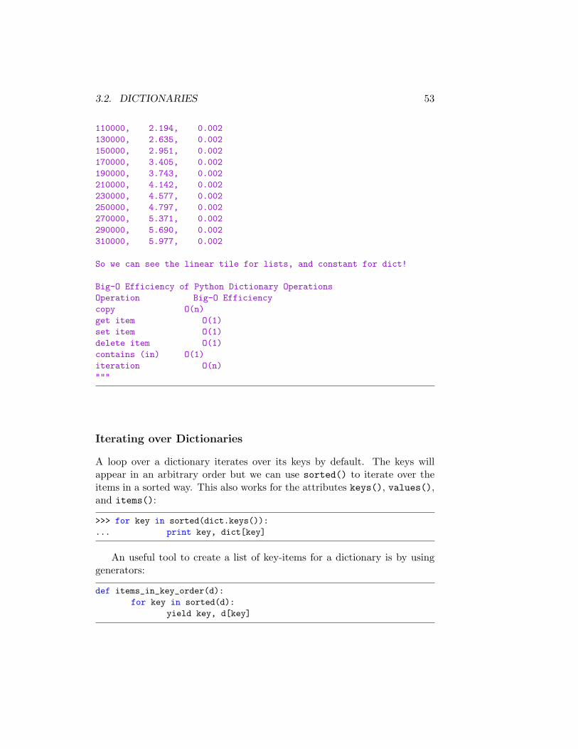
110000, 2.194, 0.002130000, 2.635, 0.002150000, 2.951, 0.002170000, 3.405, 0.002190000, 3.743, 0.002210000, 4.142, 0.002230000, 4.577, 0.002250000, 4.797, 0.002270000, 5.371, 0.002290000, 5.690, 0.002310000, 5.977, 0.002
So we can see the linear tile for lists, and constant for dict!
Big-O Efficiency of Python Dictionary OperationsOperation Big-O Efficiencycopy O(n)get item O(1)set item O(1)delete item O(1)contains (in) O(1)iteration O(n)"""
Iterating over Dictionaries
A loop over a dictionary iterates over its keys by default. The keys willappear in an arbitrary order but we can use sorted() to iterate over theitems in a sorted way. This also works for the attributes keys(), values(),and items():
>>> for key in sorted(dict.keys()):... print key, dict[key]
An useful tool to create a list of key-items for a dictionary is by usinggenerators:
def items_in_key_order(d):for key in sorted(d):
yield key, d[key]
54 CHAPTER 3. COLLECTION DATA STRUCTURES
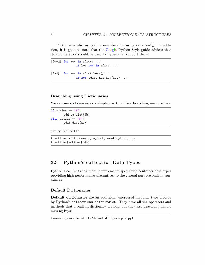
Dictionaries also support reverse iteration using reversed(). In addi-tion, it is good to note that the Google Python Style guide advices thatdefault iterators should be used for types that support them:
[Good] for key in adict: ...if key not in adict: ...
[Bad] for key in adict.keys(): ...if not adict.has_key(key): ...
Branching using Dictionaries
We can use dictionaries as a simple way to write a branching menu, where
if action == "a":add_to_dict(db)
elif action == "e":edit_dict(db)
can be reduced to
functions = dict(a=add_to_dict, e=edit_dict,...)functions[actions](db)
3.3 Python’s collection Data Types
Python’s collections module implements specialized container data typesproviding high-performance alternatives to the general purpose built-in con-tainers.
Default Dictionaries
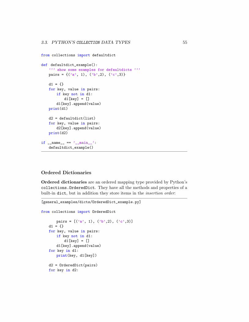
Default dictionaries are an additional unordered mapping type provideby Python’s collections.defaultdict. They have all the operators andmethods that a built-in dictionary provide, but they also gracefully handlemissing keys:
[general_examples/dicts/defaultdict_example.py]
3.3. PYTHON’S COLLECTION DATA TYPES 55
from collections import defaultdict
def defaultdict_example():’’’ show some examples for defaultdicts ’’’pairs = {(’a’, 1), (’b’,2), (’c’,3)}
d1 = {}for key, value in pairs:
if key not in d1:d1[key] = []
d1[key].append(value)print(d1)
d2 = defaultdict(list)for key, value in pairs:
d2[key].append(value)print(d2)
if __name__ == ’__main__’:defaultdict_example()
Ordered Dictionaries
Ordered dictionaries are an ordered mapping type provided by Python’scollections.OrderedDict. They have all the methods and properties of abuilt-in dict, but in addition they store items in the insertion order:
[general_examples/dicts/OrderedDict_example.py]
from collections import OrderedDict
pairs = [(’a’, 1), (’b’,2), (’c’,3)]d1 = {}for key, value in pairs:
if key not in d1:d1[key] = []
d1[key].append(value)for key in d1:
print(key, d1[key])
d2 = OrderedDict(pairs)for key in d2:
56 CHAPTER 3. COLLECTION DATA STRUCTURES
print(key, d2[key])
if __name__ == ’__main__’:OrderedDict_example()
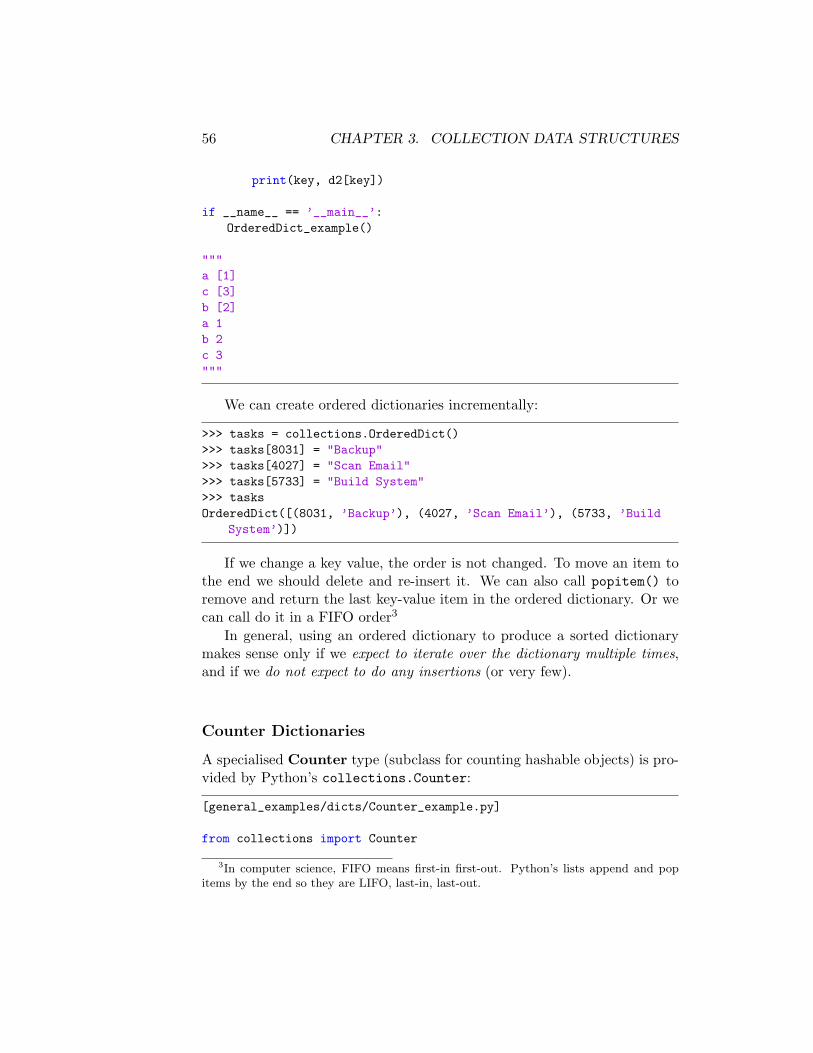
"""a [1]c [3]b [2]a 1b 2c 3"""
We can create ordered dictionaries incrementally:
>>> tasks = collections.OrderedDict()>>> tasks[8031] = "Backup">>> tasks[4027] = "Scan Email">>> tasks[5733] = "Build System">>> tasksOrderedDict([(8031, ’Backup’), (4027, ’Scan Email’), (5733, ’Build
System’)])
If we change a key value, the order is not changed. To move an item tothe end we should delete and re-insert it. We can also call popitem() toremove and return the last key-value item in the ordered dictionary. Or wecan call do it in a FIFO order3
In general, using an ordered dictionary to produce a sorted dictionarymakes sense only if we expect to iterate over the dictionary multiple times,and if we do not expect to do any insertions (or very few).
Counter Dictionaries
A specialised Counter type (subclass for counting hashable objects) is pro-vided by Python’s collections.Counter:
[general_examples/dicts/Counter_example.py]
from collections import Counter
3In computer science, FIFO means first-in first-out. Python’s lists append and popitems by the end so they are LIFO, last-in, last-out.
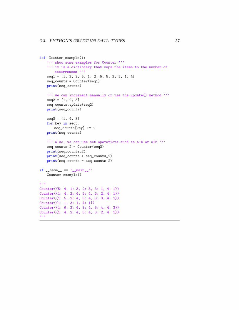
3.3. PYTHON’S COLLECTION DATA TYPES 57
def Counter_example():’’’ show some examples for Counter ’’’’’’ it is a dictionary that maps the items to the number of
occurrences ’’’seq1 = [1, 2, 3, 5, 1, 2, 5, 5, 2, 5, 1, 4]seq_counts = Counter(seq1)print(seq_counts)
’’’ we can increment manually or use the update() method ’’’seq2 = [1, 2, 3]seq_counts.update(seq2)print(seq_counts)
seq3 = [1, 4, 3]for key in seq3:
seq_counts[key] += 1print(seq_counts)
’’’ also, we can use set operations such as a-b or a+b ’’’seq_counts_2 = Counter(seq3)print(seq_counts_2)print(seq_counts + seq_counts_2)print(seq_counts - seq_counts_2)
if __name__ == ’__main__’:Counter_example()
"""Counter({5: 4, 1: 3, 2: 3, 3: 1, 4: 1})Counter({1: 4, 2: 4, 5: 4, 3: 2, 4: 1})Counter({1: 5, 2: 4, 5: 4, 3: 3, 4: 2})Counter({1: 1, 3: 1, 4: 1})Counter({1: 6, 2: 4, 3: 4, 5: 4, 4: 3})Counter({1: 4, 2: 4, 5: 4, 3: 2, 4: 1})"""
58 CHAPTER 3. COLLECTION DATA STRUCTURES
3.4 Additional Exercises
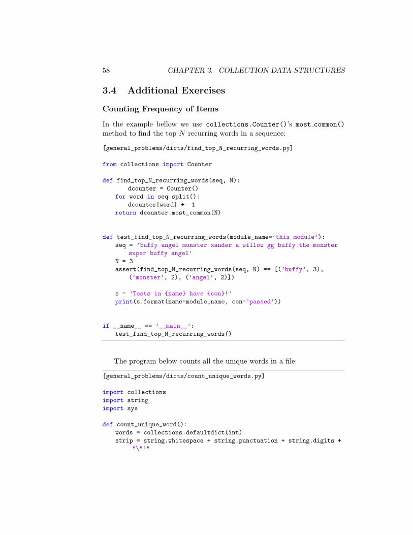
Counting Frequency of Items
In the example bellow we use collections.Counter()’s most common()method to find the top N recurring words in a sequence:
[general_problems/dicts/find_top_N_recurring_words.py]
from collections import Counter
def find_top_N_recurring_words(seq, N):dcounter = Counter()
for word in seq.split():dcounter[word] += 1
return dcounter.most_common(N)
def test_find_top_N_recurring_words(module_name=’this module’):seq = ’buffy angel monster xander a willow gg buffy the monster
super buffy angel’N = 3assert(find_top_N_recurring_words(seq, N) == [(’buffy’, 3),
(’monster’, 2), (’angel’, 2)])
s = ’Tests in {name} have {con}!’print(s.format(name=module_name, con=’passed’))
if __name__ == ’__main__’:test_find_top_N_recurring_words()
The program below counts all the unique words in a file:
[general_problems/dicts/count_unique_words.py]
import collectionsimport stringimport sys
def count_unique_word():words = collections.defaultdict(int)strip = string.whitespace + string.punctuation + string.digits +
"\"’"
3.4. ADDITIONAL EXERCISES 59
for filename in sys.argv[1:]:with open(filename) as file:
for line in file:for word in line.lower().split():
word = word.strip(strip)if len(word) > 2:
words[word] = +1for word in sorted(words):
print("’{0}’ occurs {1} times.".format(word, words[word]))
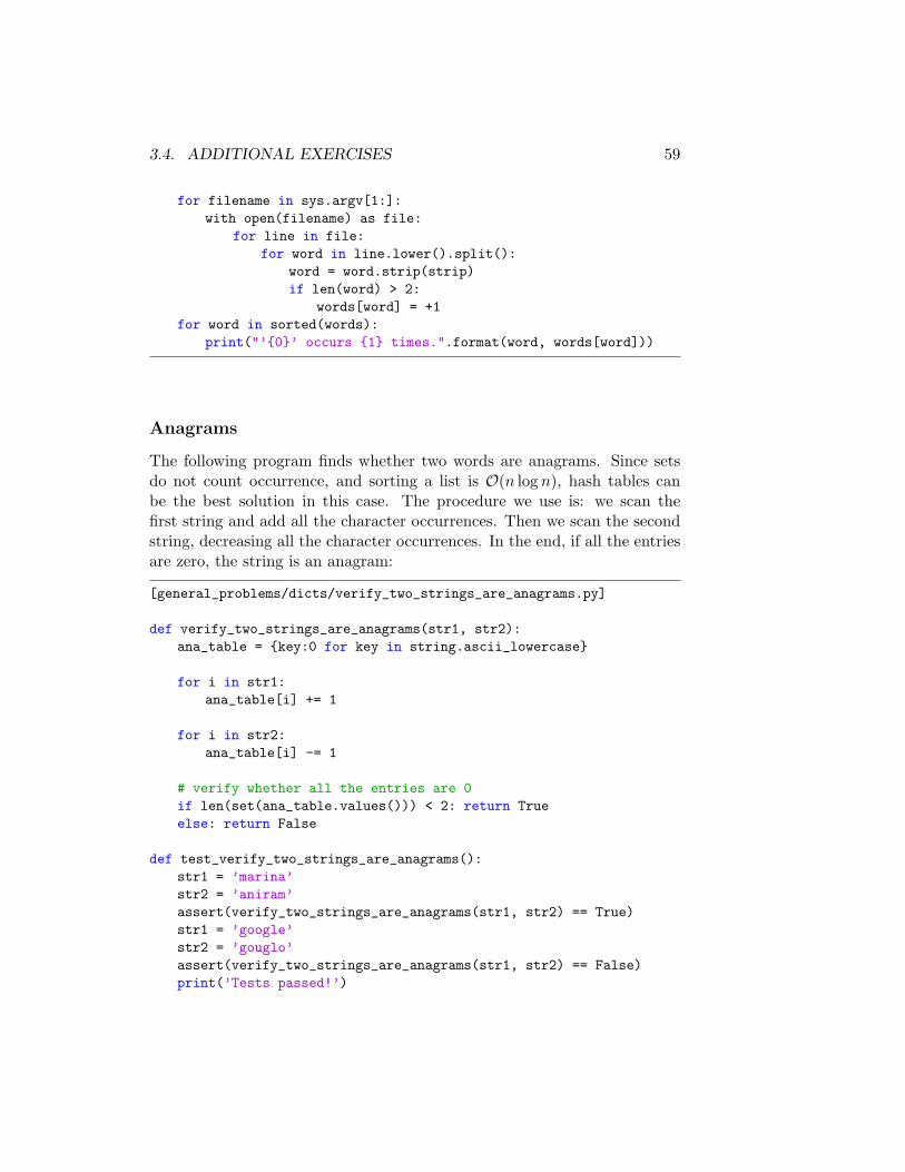
Anagrams
The following program finds whether two words are anagrams. Since setsdo not count occurrence, and sorting a list is O(n log n), hash tables canbe the best solution in this case. The procedure we use is: we scan thefirst string and add all the character occurrences. Then we scan the secondstring, decreasing all the character occurrences. In the end, if all the entriesare zero, the string is an anagram:
[general_problems/dicts/verify_two_strings_are_anagrams.py]
def verify_two_strings_are_anagrams(str1, str2):ana_table = {key:0 for key in string.ascii_lowercase}
for i in str1:ana_table[i] += 1
for i in str2:ana_table[i] -= 1
# verify whether all the entries are 0if len(set(ana_table.values())) < 2: return Trueelse: return False
def test_verify_two_strings_are_anagrams():str1 = ’marina’str2 = ’aniram’assert(verify_two_strings_are_anagrams(str1, str2) == True)str1 = ’google’str2 = ’gouglo’assert(verify_two_strings_are_anagrams(str1, str2) == False)print(’Tests passed!’)
60 CHAPTER 3. COLLECTION DATA STRUCTURES
if __name__ == ’__main__’:test_verify_two_strings_are_anagrams()
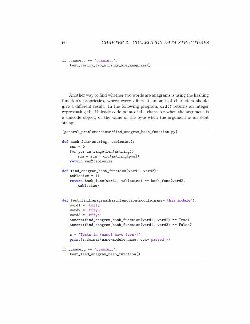
Another way to find whether two words are anagrams is using the hashingfunction’s proprieties, where every different amount of characters shouldgive a different result. In the following program, ord() returns an integerrepresenting the Unicode code point of the character when the argument isa unicode object, or the value of the byte when the argument is an 8-bitstring:
[general_problems/dicts/find_anagram_hash_function.py]
def hash_func(astring, tablesize):sum = 0for pos in range(len(astring)):
sum = sum + ord(astring[pos])return sum%tablesize
def find_anagram_hash_function(word1, word2):tablesize = 11return hash_func(word1, tablesize) == hash_func(word2,
tablesize)
def test_find_anagram_hash_function(module_name=’this module’):word1 = ’buffy’word2 = ’bffyu’word3 = ’bffya’assert(find_anagram_hash_function(word1, word2) == True)assert(find_anagram_hash_function(word1, word3) == False)
s = ’Tests in {name} have {con}!’print(s.format(name=module_name, con=’passed’))
if __name__ == ’__main__’:test_find_anagram_hash_function()
3.4. ADDITIONAL EXERCISES 61
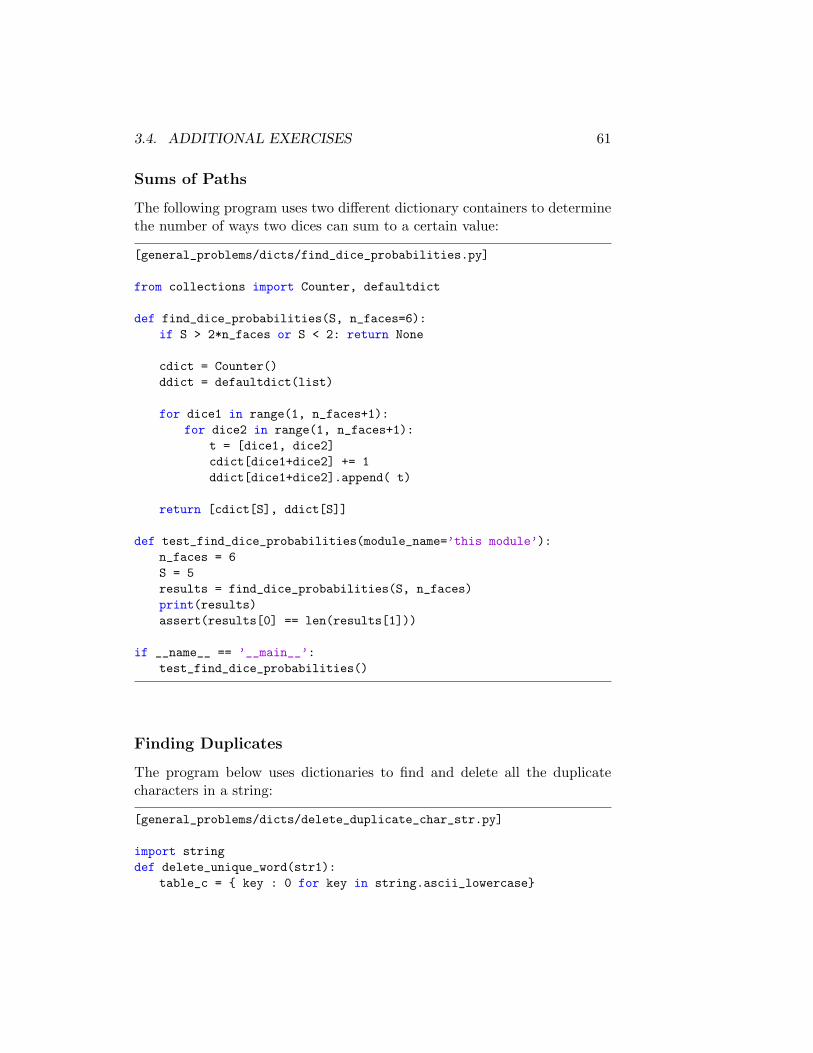
Sums of Paths
The following program uses two different dictionary containers to determinethe number of ways two dices can sum to a certain value:
[general_problems/dicts/find_dice_probabilities.py]
from collections import Counter, defaultdict
def find_dice_probabilities(S, n_faces=6):if S > 2*n_faces or S < 2: return None
cdict = Counter()ddict = defaultdict(list)
for dice1 in range(1, n_faces+1):for dice2 in range(1, n_faces+1):
t = [dice1, dice2]cdict[dice1+dice2] += 1ddict[dice1+dice2].append( t)
return [cdict[S], ddict[S]]
def test_find_dice_probabilities(module_name=’this module’):n_faces = 6S = 5results = find_dice_probabilities(S, n_faces)print(results)assert(results[0] == len(results[1]))
if __name__ == ’__main__’:test_find_dice_probabilities()
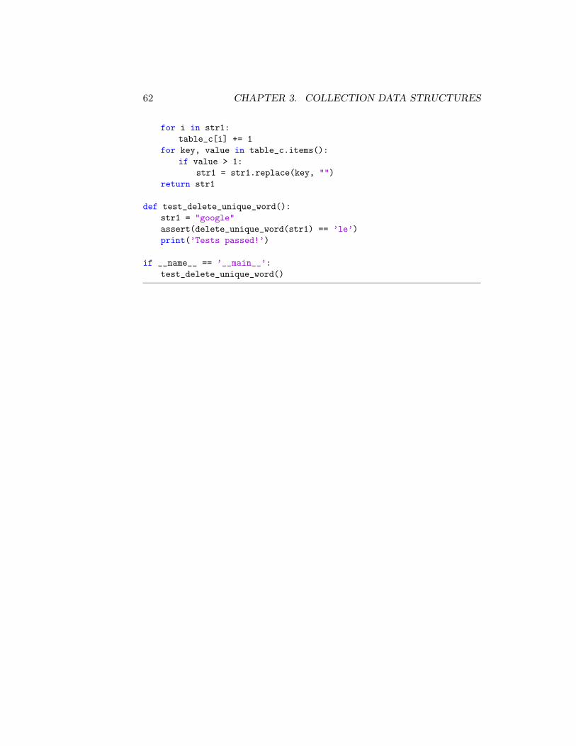
Finding Duplicates
The program below uses dictionaries to find and delete all the duplicatecharacters in a string:
[general_problems/dicts/delete_duplicate_char_str.py]
import stringdef delete_unique_word(str1):
table_c = { key : 0 for key in string.ascii_lowercase}
62 CHAPTER 3. COLLECTION DATA STRUCTURES
for i in str1:table_c[i] += 1
for key, value in table_c.items():if value > 1:
str1 = str1.replace(key, "")return str1
def test_delete_unique_word():str1 = "google"assert(delete_unique_word(str1) == ’le’)print(’Tests passed!’)
if __name__ == ’__main__’:test_delete_unique_word()
Chapter 4
Python’s Structure andModules
4.1 Modules in Python
In Python, modules are defined using the built-in name def. When def isexecuted, a function object is created together with its object reference. Ifwe do not define a return value, Python automatically returns None (likein C, we call the function a procedure when it does not return a value).
An activation record happens every time we invoke a method: informa-tion is put in the stack to support invocation. Activation records process inthe following order:
Activation Records
1. the actual parameters of the method are pushed onto the stack,
2. the return address is pushed onto the stack,
3. the top-of-stack index is incremented by the total amount required bythe local variables within the method,
4. a jump to the method.
The process of unwinding an activation record happens in the followingorder:
1. the top-of-stack index is decremented by the total amount of memoryconsumed,
63
64 CHAPTER 4. PYTHON’S STRUCTURE AND MODULES
2. the returned address is popped off the stack,
3. the top-of-stack index is decremented by the total amount of memoryby the actual parameters.
Default Values in Modules
Whenever you create a module, remember that mutable objects should notbe used as default values in the function or method definition:
[Good]def foo(a, b=None):
if b is None:b = []
[Bad]def foo(a, b=[]):
The init .py File
A package is a directory that contains a set of modules and a file calledinit .py . This is required to make Python treat the directories as
containing packages, preventing directories with a common name (such as“string”) from hiding valid modules that occur later on the module searchpath:
>>> import foldername.filemodulename
In the simplest case, it can just be an empty file, but it can also executeinitialization code for the package or set the all variable: init .pyto:
__all__ = ["file1", ...]
(with no .py in the end).Moreover, the statement:
from foldername import *
means importing every object in the module, except those whose namesbegin with , or if the module has a global all variable, the list in it.
4.1. MODULES IN PYTHON 65
Checking the Existence of a Module
To check the existence of a module, we use the flag -c:
$ python -c "import decimas"Traceback (most recent call last):File "<string>", line 1, in <module>
ImportError: No module named decimas
The name Variable
Whenever a module is imported, Python creates a variable for it calledname , and stores the module’s name in this variable. In this case, every-
thing below the statement
if __name__ == ’__main__’:
will not be executed. In the other hand, if we run the .py file directly,Python sets name to main , and every instruction following the abovestatement will be executed.
Byte-coded Compiled Modules
Byte-compiled code, in form of .pyc files, is used by the compiler to speed-upthe start-up time (load time) for short programs that use a lot of standardmodules.
When the Python interpreter is invoked with the -O flag, optimizedcode is generated and stored in .pyo files. The optimizer removes assertstatements. This also can be used to distribute a library of Python codein a form that is moderately hard to reverse engineer.
The sys Module
The variable sys.path is a list of strings that determines the interpreter’ssearch path for modules. It is initialized to a default path taken from the en-vironment variable PYTHONPATH, or from a built-in default. You can modifyit using standard list operations:
>>> import sys>>> sys.path.append( /buffy/lib/ python )
66 CHAPTER 4. PYTHON’S STRUCTURE AND MODULES
The variables sys.ps1 and sys.ps2 define the strings used as primaryand secondary prompts. The variable sys.argv allows us to use the argu-ments passed in the command line inside our programs:
import sys
def main():’’’ print command line arguments ’’’for arg in sys.argv[1:]:
print arg
if __name__ == "__main__":main()
The built-in method dir() is used to find which names a module defines(all types of names: variables, modules, functions). It returns a sorted listof strings:
>>> import sys>>> dir(sys)[ __name__ , argv , builtin_module_names , copyright ,
exit , maxint , modules , path , ps1 ,ps2 , setprofile , settrace , stderr , stdin ,stdout , version ]
It does not list the names of built-in functions and variables. Therefore,we can see that dir() is useful to find all the methods or attributes of anobject.
4.2 Control Flow
if
The if statement substitutes the switch or case statements in other lan-guages:1
>>> x = int(input("Please enter a number: "))>>> if x < 0:... x = 0... print "Negative changed to zero"
1Note that colons are used with else, elif, and in any other place where a suite is tofollow.
4.2. CONTROL FLOW 67
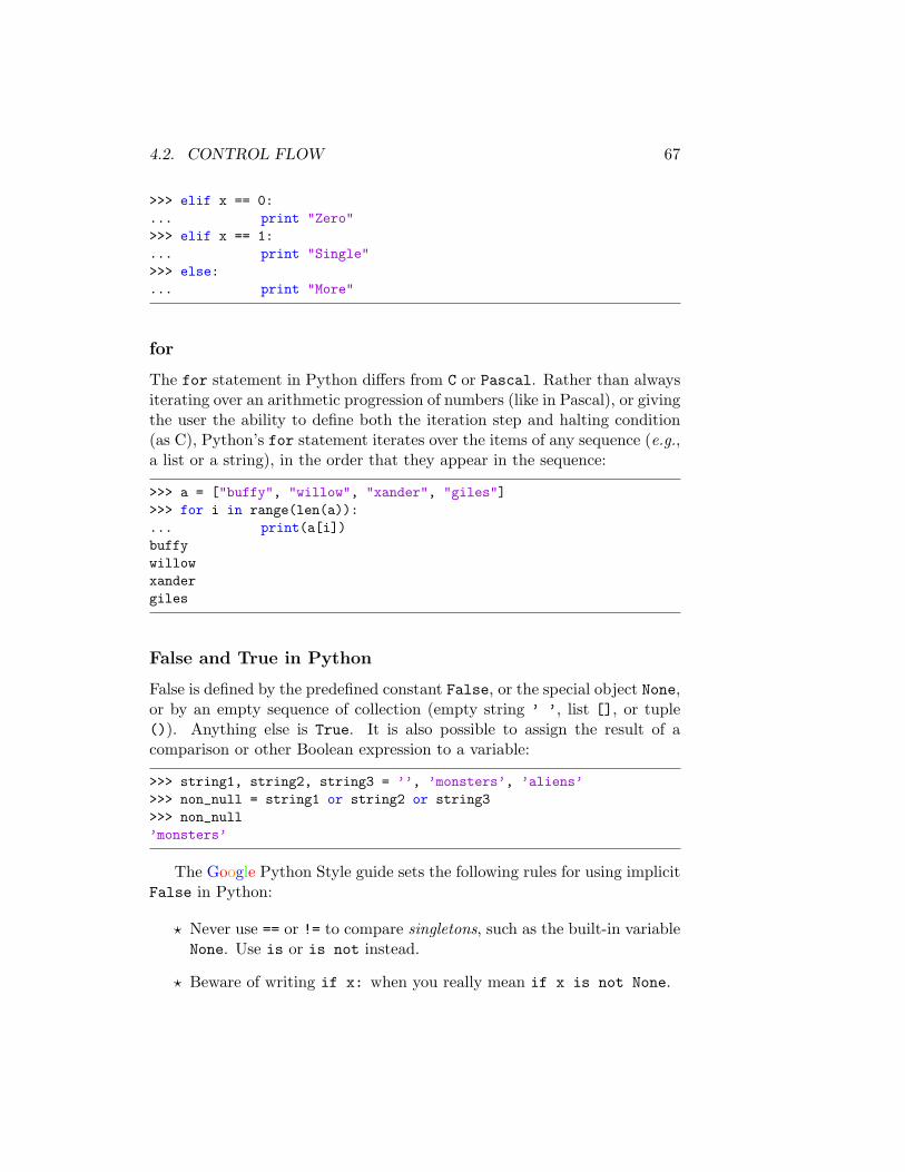
>>> elif x == 0:... print "Zero">>> elif x == 1:... print "Single">>> else:... print "More"
for
The for statement in Python differs from C or Pascal. Rather than alwaysiterating over an arithmetic progression of numbers (like in Pascal), or givingthe user the ability to define both the iteration step and halting condition(as C), Python’s for statement iterates over the items of any sequence (e.g.,a list or a string), in the order that they appear in the sequence:
>>> a = ["buffy", "willow", "xander", "giles"]>>> for i in range(len(a)):... print(a[i])buffywillowxandergiles
False and True in Python
False is defined by the predefined constant False, or the special object None,or by an empty sequence of collection (empty string ’ ’, list [], or tuple()). Anything else is True. It is also possible to assign the result of acomparison or other Boolean expression to a variable:
>>> string1, string2, string3 = ’’, ’monsters’, ’aliens’>>> non_null = string1 or string2 or string3>>> non_null’monsters’
The Google Python Style guide sets the following rules for using implicitFalse in Python:
? Never use == or != to compare singletons, such as the built-in variableNone. Use is or is not instead.
? Beware of writing if x: when you really mean if x is not None.
68 CHAPTER 4. PYTHON’S STRUCTURE AND MODULES
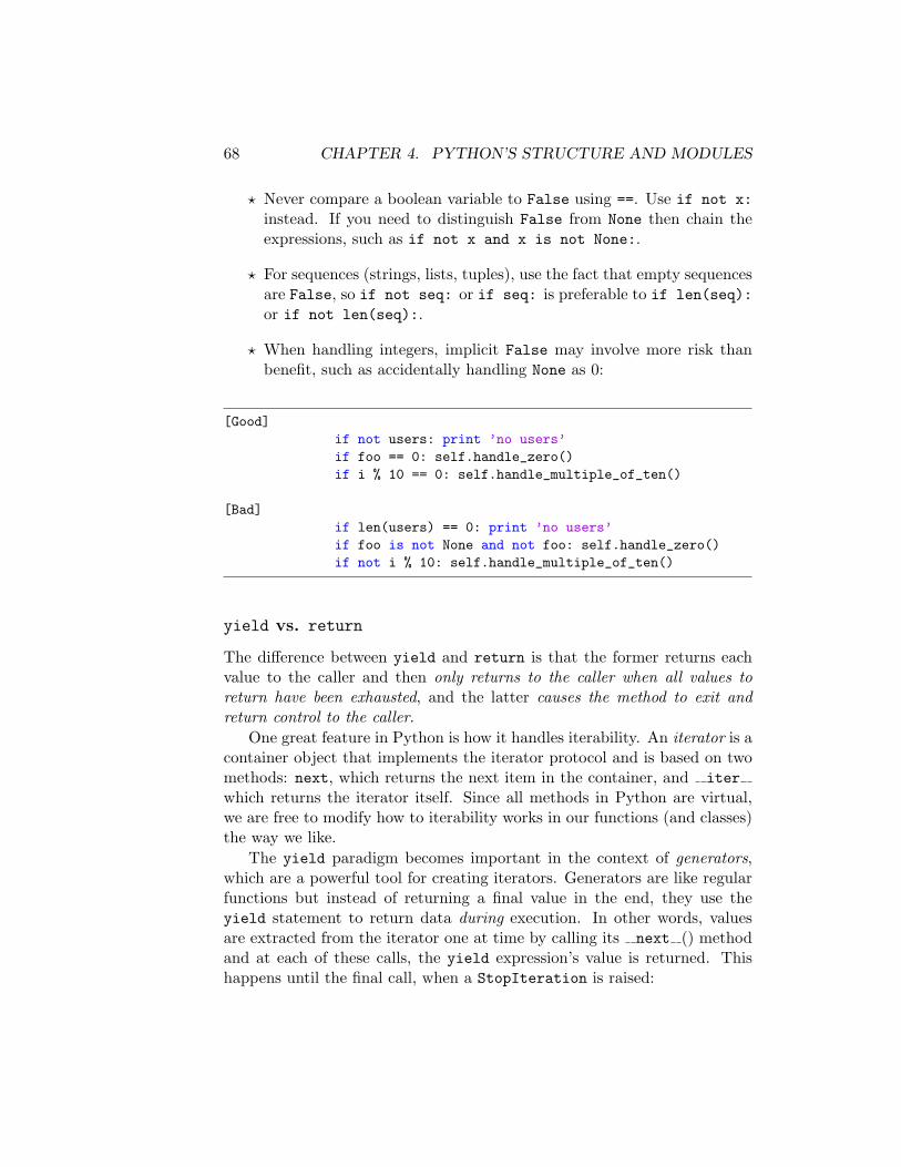
? Never compare a boolean variable to False using ==. Use if not x:instead. If you need to distinguish False from None then chain theexpressions, such as if not x and x is not None:.
? For sequences (strings, lists, tuples), use the fact that empty sequencesare False, so if not seq: or if seq: is preferable to if len(seq):or if not len(seq):.
? When handling integers, implicit False may involve more risk thanbenefit, such as accidentally handling None as 0:
[Good]if not users: print ’no users’if foo == 0: self.handle_zero()if i % 10 == 0: self.handle_multiple_of_ten()
[Bad]if len(users) == 0: print ’no users’if foo is not None and not foo: self.handle_zero()if not i % 10: self.handle_multiple_of_ten()
yield vs. return
The difference between yield and return is that the former returns eachvalue to the caller and then only returns to the caller when all values toreturn have been exhausted, and the latter causes the method to exit andreturn control to the caller.
One great feature in Python is how it handles iterability. An iterator is acontainer object that implements the iterator protocol and is based on twomethods: next, which returns the next item in the container, and iterwhich returns the iterator itself. Since all methods in Python are virtual,we are free to modify how to iterability works in our functions (and classes)the way we like.
The yield paradigm becomes important in the context of generators,which are a powerful tool for creating iterators. Generators are like regularfunctions but instead of returning a final value in the end, they use theyield statement to return data during execution. In other words, valuesare extracted from the iterator one at time by calling its next () methodand at each of these calls, the yield expression’s value is returned. Thishappens until the final call, when a StopIteration is raised:
4.2. CONTROL FLOW 69
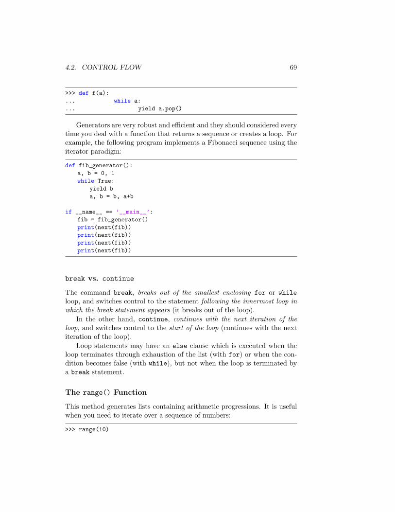
>>> def f(a):... while a:... yield a.pop()
Generators are very robust and efficient and they should considered everytime you deal with a function that returns a sequence or creates a loop. Forexample, the following program implements a Fibonacci sequence using theiterator paradigm:
def fib_generator():a, b = 0, 1while True:
yield ba, b = b, a+b
if __name__ == ’__main__’:fib = fib_generator()print(next(fib))print(next(fib))print(next(fib))print(next(fib))
break vs. continue
The command break, breaks out of the smallest enclosing for or whileloop, and switches control to the statement following the innermost loop inwhich the break statement appears (it breaks out of the loop).
In the other hand, continue, continues with the next iteration of theloop, and switches control to the start of the loop (continues with the nextiteration of the loop).
Loop statements may have an else clause which is executed when theloop terminates through exhaustion of the list (with for) or when the con-dition becomes false (with while), but not when the loop is terminated bya break statement.
The range() Function
This method generates lists containing arithmetic progressions. It is usefulwhen you need to iterate over a sequence of numbers:
>>> range(10)
70 CHAPTER 4. PYTHON’S STRUCTURE AND MODULES
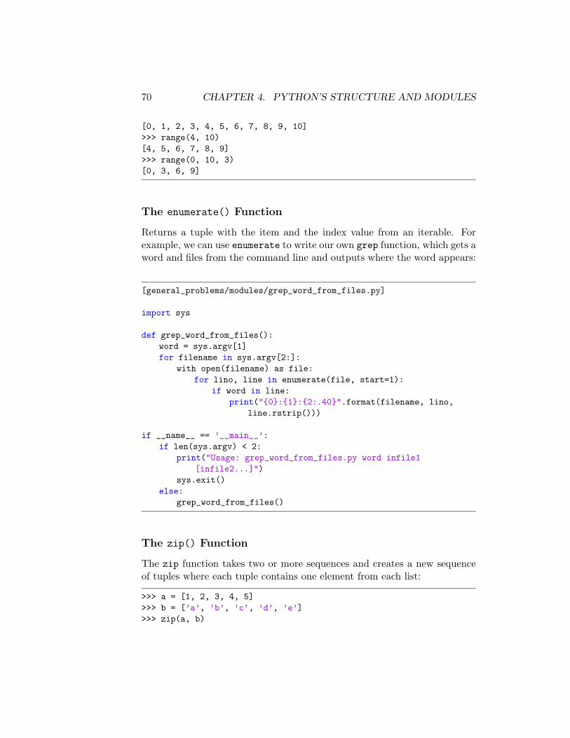
[0, 1, 2, 3, 4, 5, 6, 7, 8, 9, 10]>>> range(4, 10)[4, 5, 6, 7, 8, 9]>>> range(0, 10, 3)[0, 3, 6, 9]
The enumerate() Function
Returns a tuple with the item and the index value from an iterable. Forexample, we can use enumerate to write our own grep function, which gets aword and files from the command line and outputs where the word appears:
[general_problems/modules/grep_word_from_files.py]
import sys
def grep_word_from_files():word = sys.argv[1]for filename in sys.argv[2:]:
with open(filename) as file:for lino, line in enumerate(file, start=1):
if word in line:print("{0}:{1}:{2:.40}".format(filename, lino,
line.rstrip()))
if __name__ == ’__main__’:if len(sys.argv) < 2:
print("Usage: grep_word_from_files.py word infile1[infile2...]")
sys.exit()else:
grep_word_from_files()
The zip() Function
The zip function takes two or more sequences and creates a new sequenceof tuples where each tuple contains one element from each list:
>>> a = [1, 2, 3, 4, 5]>>> b = [’a’, ’b’, ’c’, ’d’, ’e’]>>> zip(a, b)
4.2. CONTROL FLOW 71
<zip object at 0xb72d65cc>>>> list(zip(a,b))[(1, ’a’), (2, ’b’), (3, ’c’), (4, ’d’), (5, ’e’)]
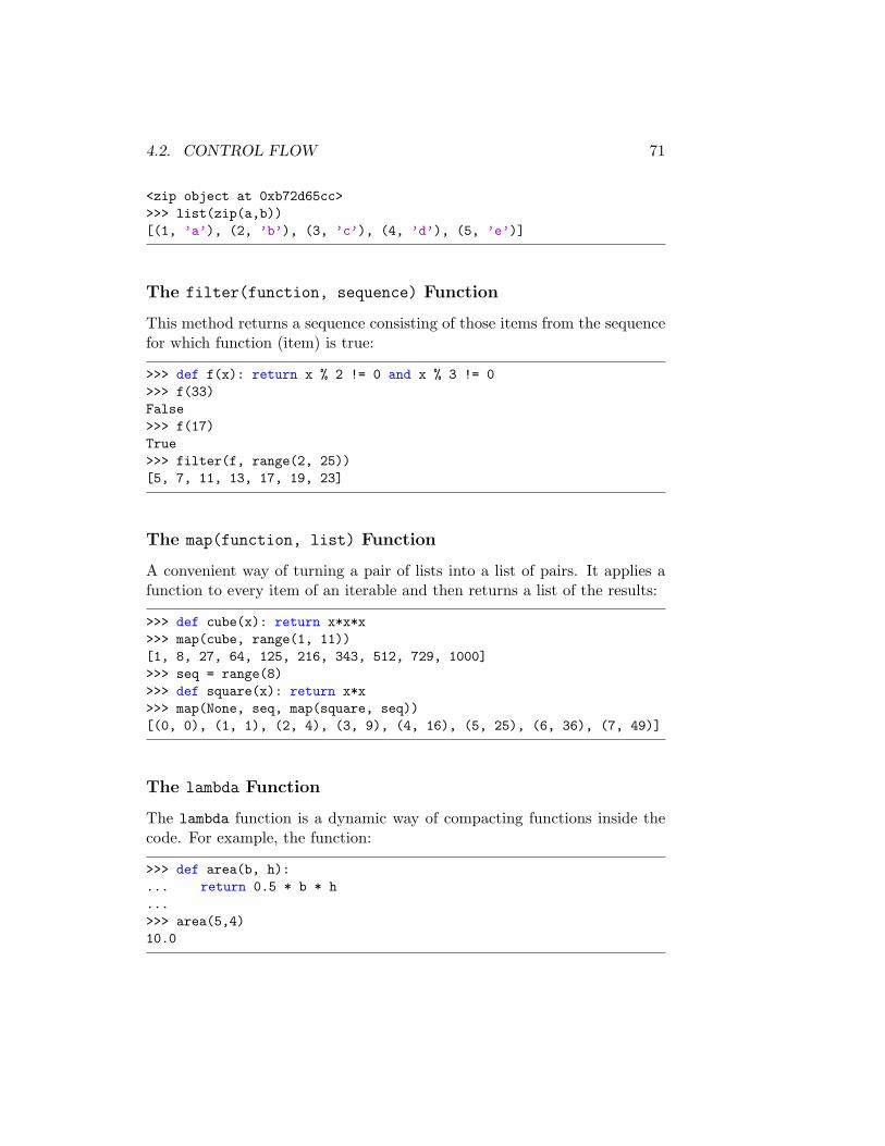
The filter(function, sequence) Function
This method returns a sequence consisting of those items from the sequencefor which function (item) is true:
>>> def f(x): return x % 2 != 0 and x % 3 != 0>>> f(33)False>>> f(17)True>>> filter(f, range(2, 25))[5, 7, 11, 13, 17, 19, 23]
The map(function, list) Function
A convenient way of turning a pair of lists into a list of pairs. It applies afunction to every item of an iterable and then returns a list of the results:
>>> def cube(x): return x*x*x>>> map(cube, range(1, 11))[1, 8, 27, 64, 125, 216, 343, 512, 729, 1000]>>> seq = range(8)>>> def square(x): return x*x>>> map(None, seq, map(square, seq))[(0, 0), (1, 1), (2, 4), (3, 9), (4, 16), (5, 25), (6, 36), (7, 49)]
The lambda Function
The lambda function is a dynamic way of compacting functions inside thecode. For example, the function:
>>> def area(b, h):... return 0.5 * b * h...>>> area(5,4)10.0
72 CHAPTER 4. PYTHON’S STRUCTURE AND MODULES
could be rather written as
>>> area = lambda b, h: 0.5 * b * h>>> area(5, 4)10.0
Lambda functions are very useful for creating keys in dictionaries:
>>> import collections>>> minus_one_dict = collections.defaultdict(lambda: -1)>>> point_zero_dict = collections.defaultdict(lambda: (0, 0))>>> message_dict = collections.defaultdict(lambda: "No message")
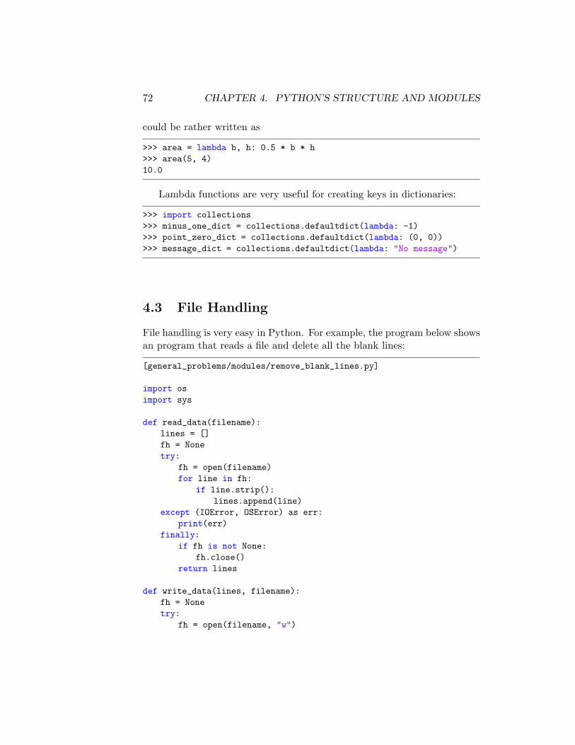
4.3 File Handling
File handling is very easy in Python. For example, the program below showsan program that reads a file and delete all the blank lines:
[general_problems/modules/remove_blank_lines.py]
import osimport sys
def read_data(filename):lines = []fh = Nonetry:
fh = open(filename)for line in fh:
if line.strip():lines.append(line)
except (IOError, OSError) as err:print(err)
finally:if fh is not None:
fh.close()return lines
def write_data(lines, filename):fh = Nonetry:
fh = open(filename, "w")
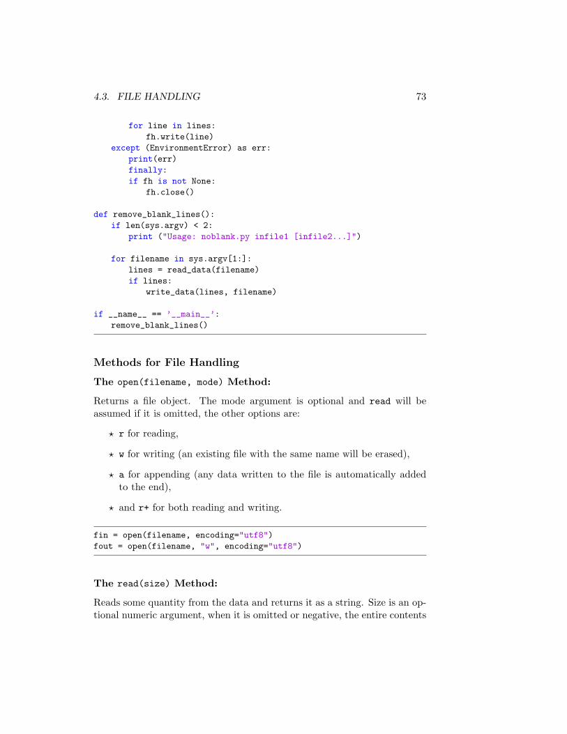
4.3. FILE HANDLING 73
for line in lines:fh.write(line)
except (EnvironmentError) as err:print(err)finally:if fh is not None:
fh.close()
def remove_blank_lines():if len(sys.argv) < 2:
print ("Usage: noblank.py infile1 [infile2...]")
for filename in sys.argv[1:]:lines = read_data(filename)if lines:
write_data(lines, filename)
if __name__ == ’__main__’:remove_blank_lines()
Methods for File Handling
The open(filename, mode) Method:
Returns a file object. The mode argument is optional and read will beassumed if it is omitted, the other options are:
? r for reading,
? w for writing (an existing file with the same name will be erased),
? a for appending (any data written to the file is automatically addedto the end),
? and r+ for both reading and writing.
fin = open(filename, encoding="utf8")fout = open(filename, "w", encoding="utf8")
The read(size) Method:
Reads some quantity from the data and returns it as a string. Size is an op-tional numeric argument, when it is omitted or negative, the entire contents
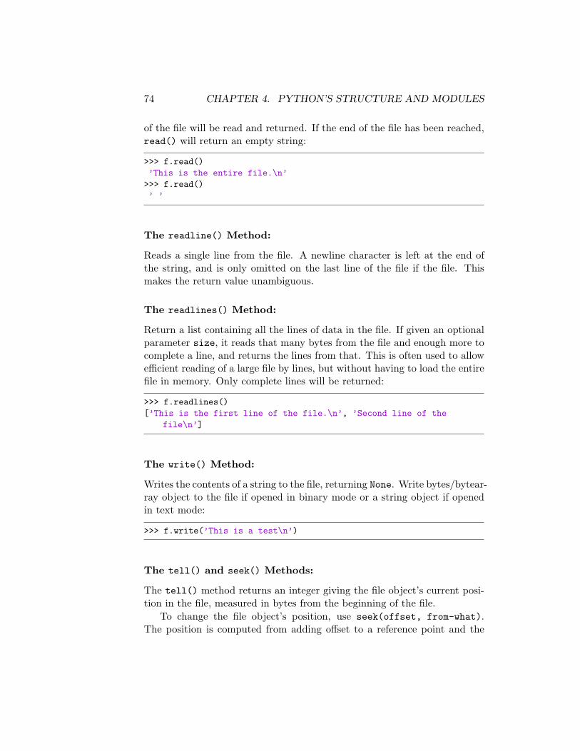
74 CHAPTER 4. PYTHON’S STRUCTURE AND MODULES
of the file will be read and returned. If the end of the file has been reached,read() will return an empty string:
>>> f.read()’This is the entire file.\n’>>> f.read()’ ’
The readline() Method:
Reads a single line from the file. A newline character is left at the end ofthe string, and is only omitted on the last line of the file if the file. Thismakes the return value unambiguous.
The readlines() Method:
Return a list containing all the lines of data in the file. If given an optionalparameter size, it reads that many bytes from the file and enough more tocomplete a line, and returns the lines from that. This is often used to allowefficient reading of a large file by lines, but without having to load the entirefile in memory. Only complete lines will be returned:
>>> f.readlines()[’This is the first line of the file.\n’, ’Second line of the
file\n’]
The write() Method:
Writes the contents of a string to the file, returning None. Write bytes/bytear-ray object to the file if opened in binary mode or a string object if openedin text mode:
>>> f.write(’This is a test\n’)
The tell() and seek() Methods:
The tell() method returns an integer giving the file object’s current posi-tion in the file, measured in bytes from the beginning of the file.
To change the file object’s position, use seek(offset, from-what).The position is computed from adding offset to a reference point and the
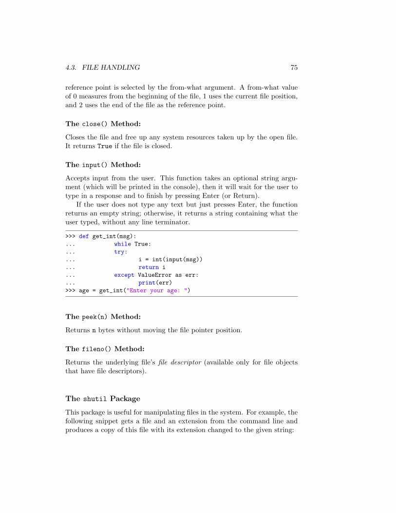
4.3. FILE HANDLING 75
reference point is selected by the from-what argument. A from-what valueof 0 measures from the beginning of the file, 1 uses the current file position,and 2 uses the end of the file as the reference point.
The close() Method:
Closes the file and free up any system resources taken up by the open file.It returns True if the file is closed.
The input() Method:
Accepts input from the user. This function takes an optional string argu-ment (which will be printed in the console), then it will wait for the user totype in a response and to finish by pressing Enter (or Return).
If the user does not type any text but just presses Enter, the functionreturns an empty string; otherwise, it returns a string containing what theuser typed, without any line terminator.
>>> def get_int(msg):... while True:... try:... i = int(input(msg))... return i... except ValueError as err:... print(err)>>> age = get_int("Enter your age: ")
The peek(n) Method:
Returns n bytes without moving the file pointer position.
The fileno() Method:
Returns the underlying file’s file descriptor (available only for file objectsthat have file descriptors).
The shutil Package
This package is useful for manipulating files in the system. For example, thefollowing snippet gets a file and an extension from the command line andproduces a copy of this file with its extension changed to the given string:
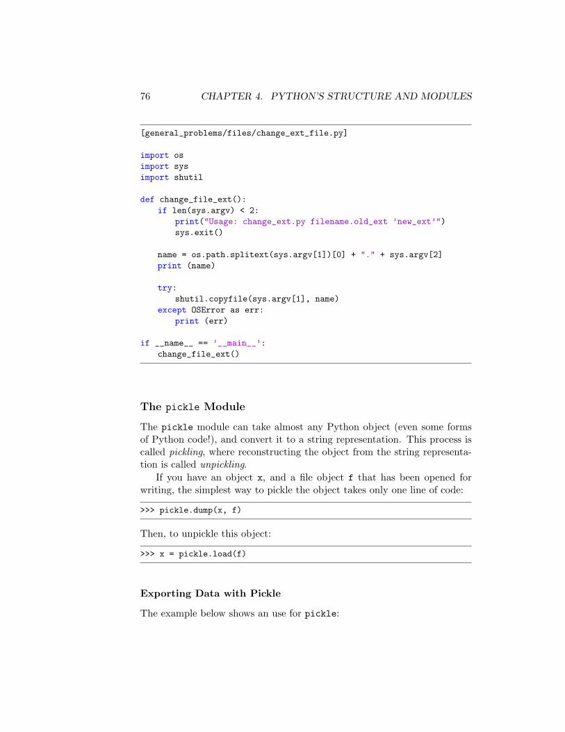
76 CHAPTER 4. PYTHON’S STRUCTURE AND MODULES
[general_problems/files/change_ext_file.py]
import osimport sysimport shutil
def change_file_ext():if len(sys.argv) < 2:
print("Usage: change_ext.py filename.old_ext ’new_ext’")sys.exit()
name = os.path.splitext(sys.argv[1])[0] + "." + sys.argv[2]print (name)
try:shutil.copyfile(sys.argv[1], name)
except OSError as err:print (err)
if __name__ == ’__main__’:change_file_ext()
The pickle Module
The pickle module can take almost any Python object (even some formsof Python code!), and convert it to a string representation. This process iscalled pickling, where reconstructing the object from the string representa-tion is called unpickling.
If you have an object x, and a file object f that has been opened forwriting, the simplest way to pickle the object takes only one line of code:
>>> pickle.dump(x, f)
Then, to unpickle this object:
>>> x = pickle.load(f)
Exporting Data with Pickle
The example below shows an use for pickle:
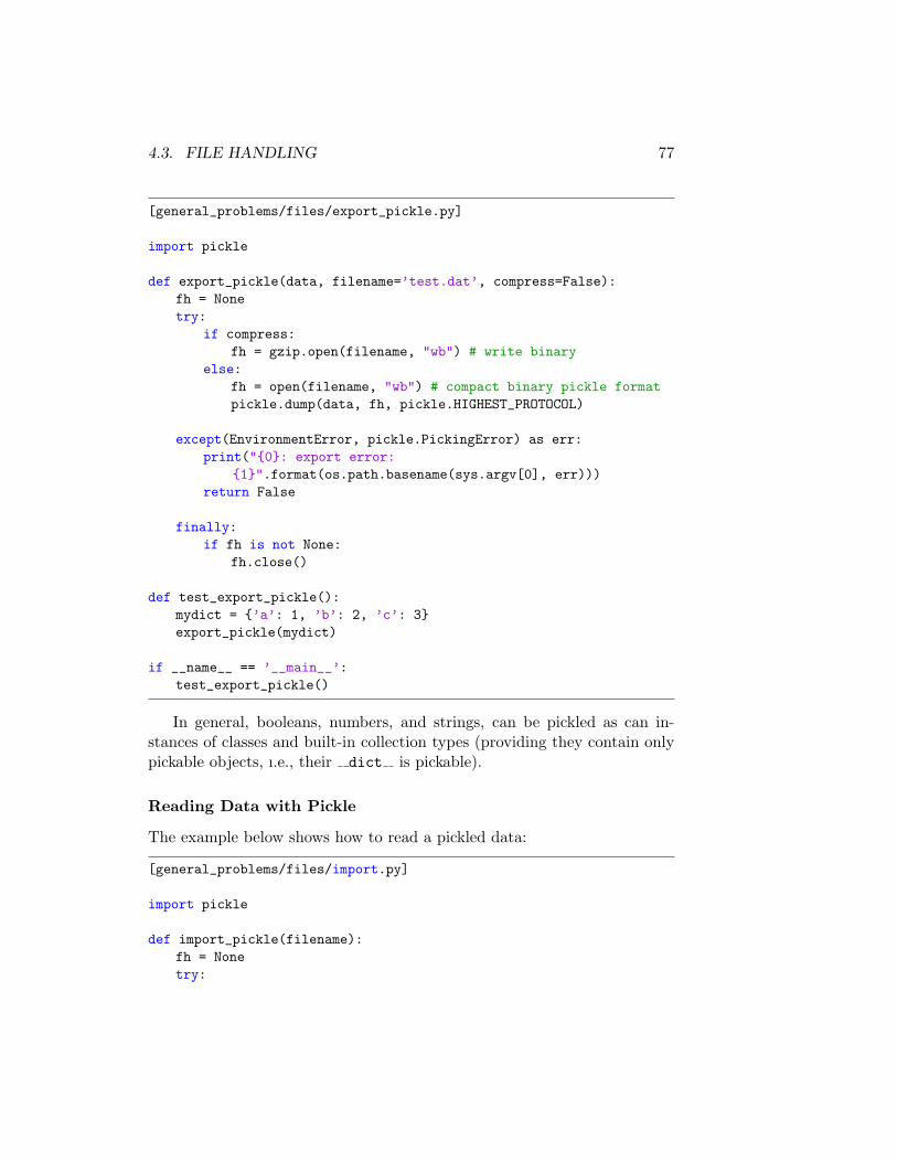
4.3. FILE HANDLING 77
[general_problems/files/export_pickle.py]
import pickle
def export_pickle(data, filename=’test.dat’, compress=False):fh = Nonetry:
if compress:fh = gzip.open(filename, "wb") # write binary
else:fh = open(filename, "wb") # compact binary pickle formatpickle.dump(data, fh, pickle.HIGHEST_PROTOCOL)
except(EnvironmentError, pickle.PickingError) as err:print("{0}: export error:
{1}".format(os.path.basename(sys.argv[0], err)))return False
finally:if fh is not None:
fh.close()
def test_export_pickle():mydict = {’a’: 1, ’b’: 2, ’c’: 3}export_pickle(mydict)
if __name__ == ’__main__’:test_export_pickle()
In general, booleans, numbers, and strings, can be pickled as can in-stances of classes and built-in collection types (providing they contain onlypickable objects, ı.e., their dict is pickable).
Reading Data with Pickle
The example below shows how to read a pickled data:
[general_problems/files/import.py]
import pickle
def import_pickle(filename):fh = Nonetry:
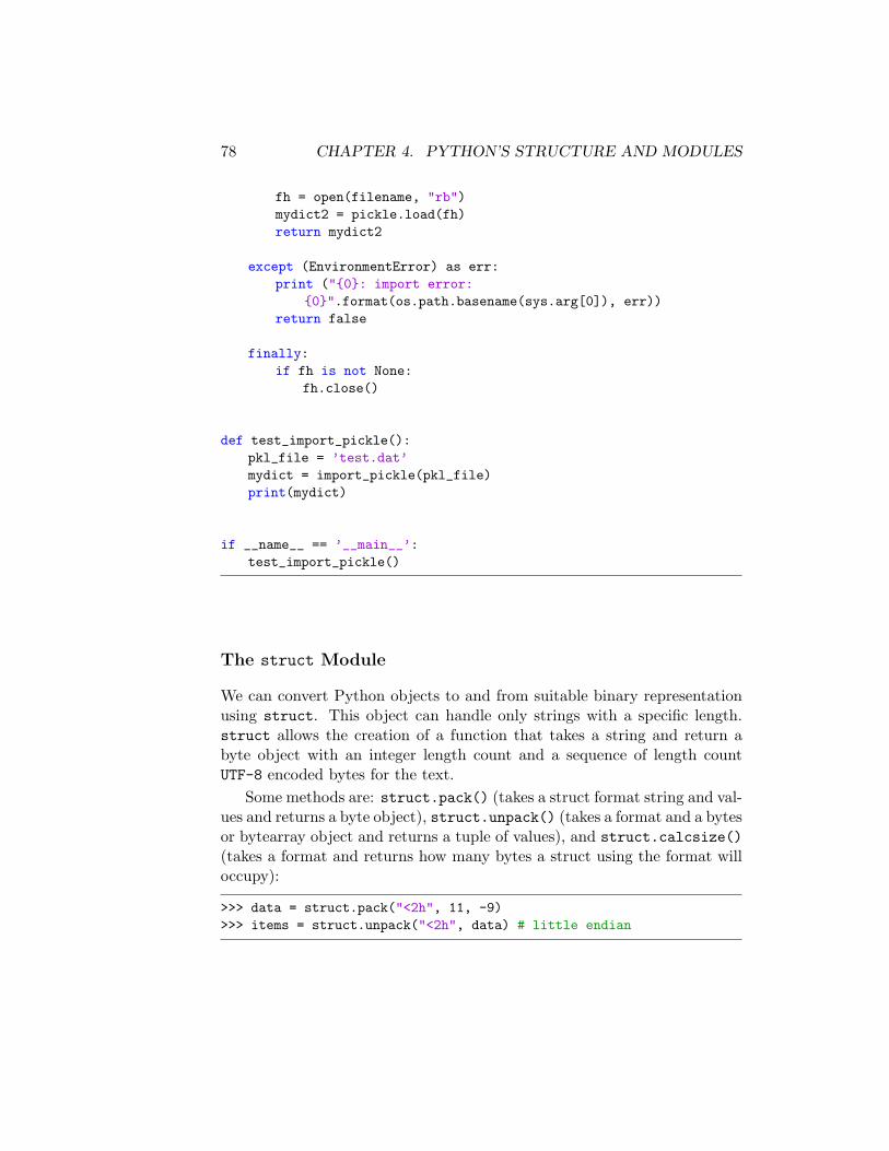
78 CHAPTER 4. PYTHON’S STRUCTURE AND MODULES
fh = open(filename, "rb")mydict2 = pickle.load(fh)return mydict2
except (EnvironmentError) as err:print ("{0}: import error:
{0}".format(os.path.basename(sys.arg[0]), err))return false
finally:if fh is not None:
fh.close()
def test_import_pickle():pkl_file = ’test.dat’mydict = import_pickle(pkl_file)print(mydict)
if __name__ == ’__main__’:test_import_pickle()
The struct Module
We can convert Python objects to and from suitable binary representationusing struct. This object can handle only strings with a specific length.struct allows the creation of a function that takes a string and return abyte object with an integer length count and a sequence of length countUTF-8 encoded bytes for the text.
Some methods are: struct.pack() (takes a struct format string and val-ues and returns a byte object), struct.unpack() (takes a format and a bytesor bytearray object and returns a tuple of values), and struct.calcsize()(takes a format and returns how many bytes a struct using the format willoccupy):
>>> data = struct.pack("<2h", 11, -9)>>> items = struct.unpack("<2h", data) # little endian
4.4. MULTIPROCESSING AND THREADING 79
4.4 Multiprocessing and Threading
Each program in the operational system is a separate process. Each processhas one or more threads. If a process has several threads, they appear torun simultaneously. Two approaches can be used to spread the workload inprograms:
Multiple processes Multiple processes have separate regions of memoryand can only communicate by special mechanisms. The processorloads and saves a separate set of registers for each thread. It is incon-venient for communication and data sharing. This is handled by thesubprocess module.
Multiple threads Multiple threads in a single process have access to thesame memory. They communicate simply by sharing data, provid-ing ensure of one thread at time, handled by the threading module.Threads share the process’s resources, including the heap space. Buteach thread still has it own stack.
Although Python has a threading mechanism, it does not support trueparallel execution. However, it is possible is to use parallel processes, whichin modern operating systems are really efficient.
The subprocess Module
Used to create a pair of “parent-child” programs, where the parent programis run by the user and this in turn runs as many instances of the childprogram, each with different work to do. Using child processing allow usto take maximum advantage of multicore processor and leaves concurrencyissues to be handled by the operational system.
The threading Module
The complexity arises when we want to separate threads to share data, andwe need to be careful with a policy for locks and for avoiding deadlocks.Each Python program has at least one thread, the main thread. To createmultiple threads we use the threading module::
? calling threading.thread() and passing a callable object,
? calling threading.threadclass and threading.threadsubclass.
80 CHAPTER 4. PYTHON’S STRUCTURE AND MODULES
The queue.queue class can handle all the locking internally: we can relyon it to serialize accesses, meaning that only one thread at time has accessto the data (FIFO). The program will not terminate while it has any threadsrunning.
It might create a problem since once the worker threads have done theirwork, they are finished but they are technically still running. The solu-tion is to transform threads into daemons. In this case, the program willterminate as soon as there is no daemon threads running. The methodqueue.queue.join() blocks the end until the queue is empty.
Mutexes and Semaphores
A mutex is like a lock. Mutexes are used in parallel programming to ensurethat only one thread can access a shared resource at a time. For example,say one thread is modifying an array. When it has gotten halfway throughthe array, the processor switches to another thread. If we were not usingmutexes, the thread could try to modify the array as well, which is probablynot what we want.
Conceptually, a mutex is an integer that starts at 1. Whenever a threadneeds to alter the array, it “locks” the mutex. This causes the thread to waituntil the number is positive and then decreases it by one. When the threadis done modifying the array, it “unlocks” the mutex, causing the number toincrease by 1. If we are sure to lock the mutex before modifying the arrayand to unlock it when we are done, then we know that no two threads willmodify the array at the same time.
Semaphores are more general than mutexes. A semaphore’s integer maystart at a number greater than 1. The number at which a semaphore startsis the number of threads that may access the resource at once. Semaphoressupport “wait” and “signal” operations, which are analogous to the “lock”and “unlock” operations of mutexes.
Deadlock and Spinlock
Deadlock is a problem that sometimes arises in parallel programming, whentwo threads are stuck indefinitely. We can prevent deadlock if we assign anorder to our locks and require that locks will always be acquired in order(this is a very general and not precise approach).
Spinlock is a form of busy waiting, that can be useful for high-performancecomputing (HPC) (when the entire system is dedicated to a single applica-tion and exactly one thread per core). It takes less time than a semaphore.
4.5. ERROR HANDLING IN PYTHON 81
The Google Python Style Guide for Threading
Google warns to not rely on the atomicity of built-in types (data types suchas dictionaries appear to have atomic operations, but they are actually basedon private methods such as hash or eq ). Queue module’s data typeas the preferred way to communicate data between threads. Otherwise, usethe threading module and its locking primitives.
4.5 Error Handling in Python
There are two distinguishable kinds of errors when we compile a programin Python: syntax errors (parsing errors) and exceptions (errors detectedduring execution, not unconditionally fatal). While syntax errors will neverallow the program to be compiled, exceptions can only be detected in somecases and for this reason they should be carefully handled.
Handling Exceptions
When an exception is raised and not handled, Python outputs a tracebackalong with the exception’s error message. A traceback (sometimes called abacktrace) is a list of all the calls made from the point where the unhandledexception occurred back to the top of the call stack.
We can handle predictable exceptions by using the try-except-finallyparadigm:
try:try_suite
except exception1 as variable1:exception_suite1
...except exceptionN as variableN:
exception_suiteN
If the statements in the try block’s suite are all executed without raisingan exception, the except blocks are skipped. If an exception is raised insidethe try block, control is immediately passed to the suite corresponding tothe first matching exception. This means that any statements in the suitethat follow the one that caused the exception will not be executed:
while 1:try:
82 CHAPTER 4. PYTHON’S STRUCTURE AND MODULES
x = int(raw_input("Please enter a number: "))break
except ValueError:print "Oops! That was no valid number. Try again..."
The raise statement allows the programmer to force a specified excep-tion to occur:
import stringimport systry:
f = open(’myfile.txt’)s = f.readline()i = int(string.strip(s))
except IOError, (errno, strerror):print "I/O error(%s): %s" % (errno, strerror)
except ValueError:print "Could not convert data to an integer."
except:print "Unexpected error:", sys.exc_info()[0]raise
We also can use else:
for arg in sys.argv[1:]:try:
f = open(arg, ’r’)except IOError:
print ’cannot open’, argelse:
print arg, ’has’, len(f.readlines()), ’lines’f.close()
The Google Python Style Guide for Exceptions
Exceptions must be used carefully and must follow certain conditions:
? Raise exceptions like this: raise MyException(’Error message’) orraise MyException. Do not use the two-argument form.
? Modules or packages should define their own domain-specific base ex-ception class, which should be inherit from the built-in Exceptionclass. The base exception for a module should be called Error.
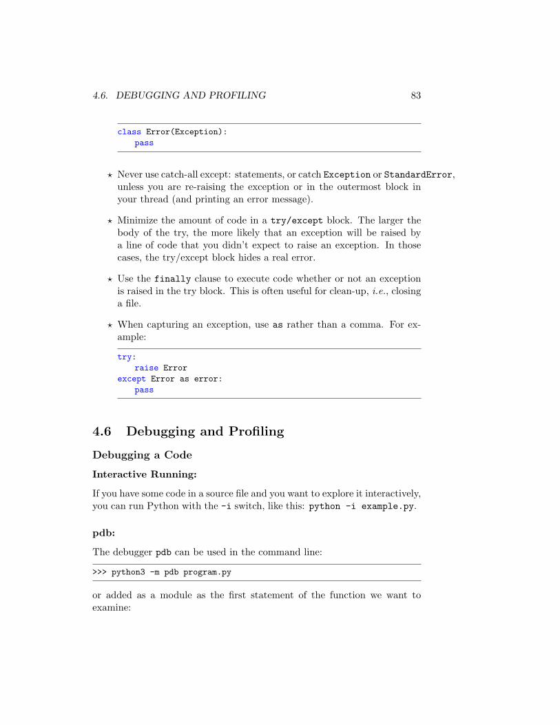
4.6. DEBUGGING AND PROFILING 83
class Error(Exception):pass
? Never use catch-all except: statements, or catch Exception or StandardError,unless you are re-raising the exception or in the outermost block inyour thread (and printing an error message).
? Minimize the amount of code in a try/except block. The larger thebody of the try, the more likely that an exception will be raised bya line of code that you didn’t expect to raise an exception. In thosecases, the try/except block hides a real error.
? Use the finally clause to execute code whether or not an exceptionis raised in the try block. This is often useful for clean-up, i.e., closinga file.
? When capturing an exception, use as rather than a comma. For ex-ample:
try:raise Error
except Error as error:pass
4.6 Debugging and Profiling
Debugging a Code
Interactive Running:
If you have some code in a source file and you want to explore it interactively,you can run Python with the -i switch, like this: python -i example.py.
pdb:
The debugger pdb can be used in the command line:
>>> python3 -m pdb program.py
or added as a module as the first statement of the function we want toexamine:
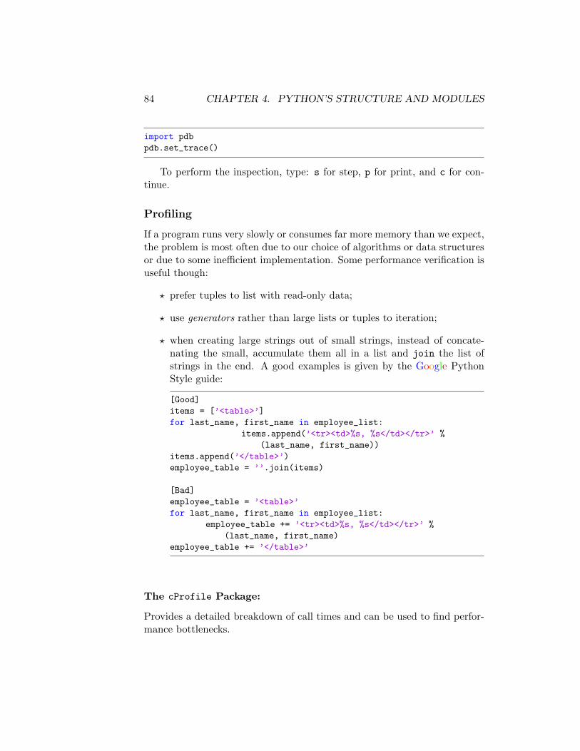
84 CHAPTER 4. PYTHON’S STRUCTURE AND MODULES
import pdbpdb.set_trace()
To perform the inspection, type: s for step, p for print, and c for con-tinue.
Profiling
If a program runs very slowly or consumes far more memory than we expect,the problem is most often due to our choice of algorithms or data structuresor due to some inefficient implementation. Some performance verification isuseful though:
? prefer tuples to list with read-only data;
? use generators rather than large lists or tuples to iteration;
? when creating large strings out of small strings, instead of concate-nating the small, accumulate them all in a list and join the list ofstrings in the end. A good examples is given by the Google PythonStyle guide:
[Good]items = [’<table>’]for last_name, first_name in employee_list:
items.append(’<tr><td>%s, %s</td></tr>’ %(last_name, first_name))
items.append(’</table>’)employee_table = ’’.join(items)
[Bad]employee_table = ’<table>’for last_name, first_name in employee_list:
employee_table += ’<tr><td>%s, %s</td></tr>’ %(last_name, first_name)
employee_table += ’</table>’
The cProfile Package:
Provides a detailed breakdown of call times and can be used to find perfor-mance bottlenecks.
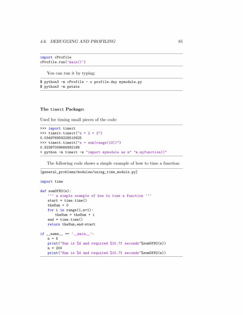
4.6. DEBUGGING AND PROFILING 85
import cProfilecProfile.run(’main()’)
You can run it by typing:
$ python3 -m cProfile - o profile.day mymodule.py$ python3 -m pstats
The timeit Package:
Used for timing small pieces of the code:
>>> import timeit>>> timeit.timeit("x = 2 + 2")0.034976959228515625>>> timeit.timeit("x = sum(range(10))")0.92387008666992188> python -m timeit -s "import mymodule as m" "m.myfunction()"
The following code shows a simple example of how to time a function:
[general_problems/modules/using_time_module.py]
import time
def sumOfN2(n):’’’ a simple example of how to time a function ’’’start = time.time()theSum = 0for i in range(1,n+1):
theSum = theSum + iend = time.time()return theSum,end-start
if __name__ == ’__main__’:n = 5print("Sum is %d and required %10.7f seconds"%sumOfN2(n))n = 200print("Sum is %d and required %10.7f seconds"%sumOfN2(n))
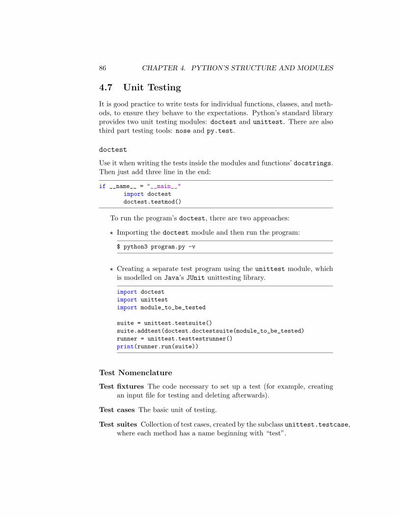
86 CHAPTER 4. PYTHON’S STRUCTURE AND MODULES
4.7 Unit Testing
It is good practice to write tests for individual functions, classes, and meth-ods, to ensure they behave to the expectations. Python’s standard libraryprovides two unit testing modules: doctest and unittest. There are alsothird part testing tools: nose and py.test.
doctest
Use it when writing the tests inside the modules and functions’ docstrings.Then just add three line in the end:
if __name__ = "__main__"import doctestdoctest.testmod()
To run the program’s doctest, there are two approaches:
? Importing the doctest module and then run the program:
$ python3 program.py -v
? Creating a separate test program using the unittest module, whichis modelled on Java’s JUnit unittesting library.
import doctestimport unittestimport module_to_be_tested
suite = unittest.testsuite()suite.addtest(doctest.doctestsuite(module_to_be_tested)runner = unittest.testtestrunner()print(runner.run(suite))
Test Nomenclature
Test fixtures The code necessary to set up a test (for example, creatingan input file for testing and deleting afterwards).
Test cases The basic unit of testing.
Test suites Collection of test cases, created by the subclass unittest.testcase,where each method has a name beginning with “test”.
4.7. UNIT TESTING 87
Test runner An object that executes one of more test suites.
88 CHAPTER 4. PYTHON’S STRUCTURE AND MODULES
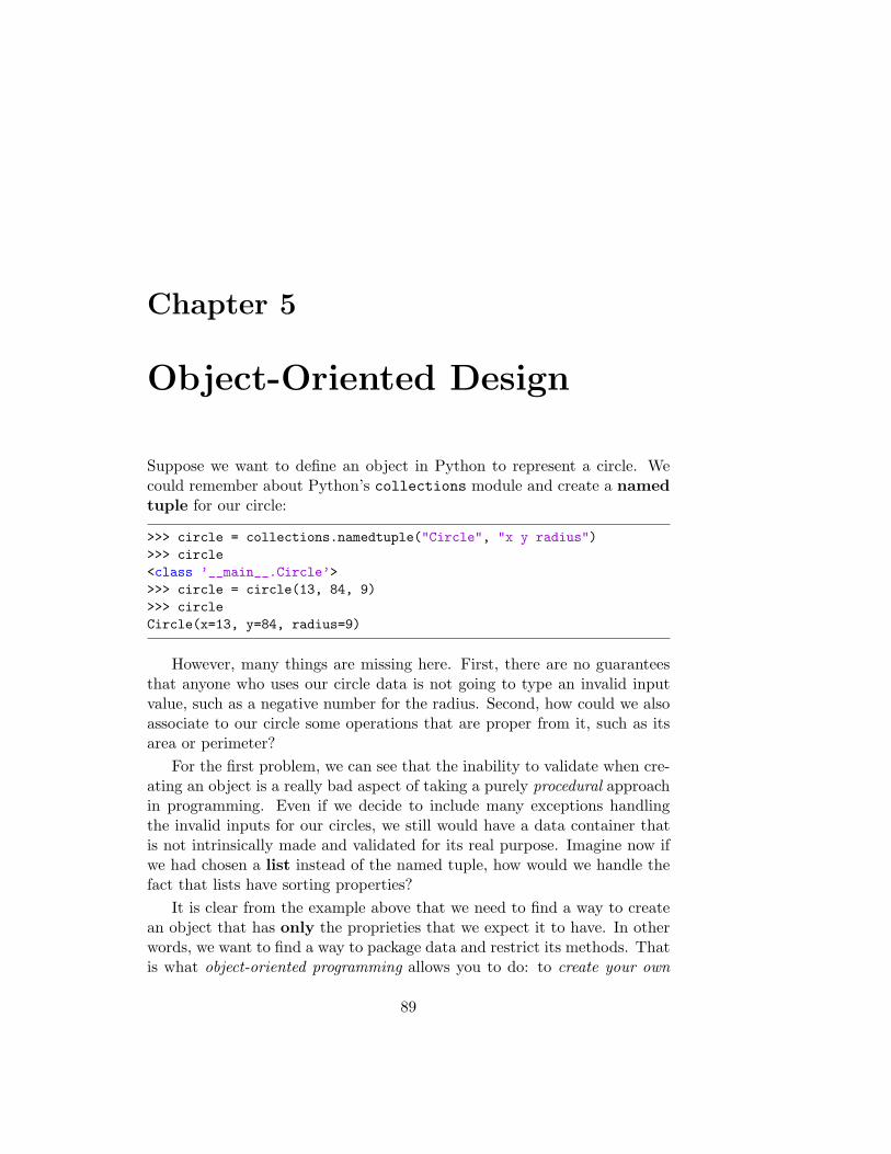
Chapter 5
Object-Oriented Design
Suppose we want to define an object in Python to represent a circle. Wecould remember about Python’s collections module and create a namedtuple for our circle:
>>> circle = collections.namedtuple("Circle", "x y radius")>>> circle<class ’__main__.Circle’>>>> circle = circle(13, 84, 9)>>> circleCircle(x=13, y=84, radius=9)
However, many things are missing here. First, there are no guaranteesthat anyone who uses our circle data is not going to type an invalid inputvalue, such as a negative number for the radius. Second, how could we alsoassociate to our circle some operations that are proper from it, such as itsarea or perimeter?
For the first problem, we can see that the inability to validate when cre-ating an object is a really bad aspect of taking a purely procedural approachin programming. Even if we decide to include many exceptions handlingthe invalid inputs for our circles, we still would have a data container thatis not intrinsically made and validated for its real purpose. Imagine now ifwe had chosen a list instead of the named tuple, how would we handle thefact that lists have sorting properties?
It is clear from the example above that we need to find a way to createan object that has only the proprieties that we expect it to have. In otherwords, we want to find a way to package data and restrict its methods. Thatis what object-oriented programming allows you to do: to create your own
89
90 CHAPTER 5. OBJECT-ORIENTED DESIGN
custom data type, which in this example would be a circle class.
5.1 Classes and Objects
Classes are the way we can gather special predefined data and methods to-gether. We use them by creating objects, which are instances of a particularclass. The simplest form of a class in Python looks like the following snippet:
class ClassName:<statement-1>.g<statement-N>
>>> x = ClassName() # class instantiation
Class Instantiation
Class instantiation uses function notation to create objects in a known ini-tial state. The instantiation operation creates an empty object which hasindividuality. However, multiple names (in multiple scopes) can be boundto the same object (also know as aliasing). In Python, when an object iscreated, first the special method new () is called (the constructor) andthen init () initializes it.
Attributes
Objects have the attributes from their Classes, which are methods and data.Method attributes are functions whose first argument is the instance onwhich it is called to operate (which in Python is conventionally called self).
Attributes are any name following a dot. References to names in modulesare attribute references: in the expression modname.funcname, modname isa module object and funcname is one of its attribute. Attributes may beread-only or writeable. Writeable attributes may be deleted with the delstatement.
Namespaces
A namespace is a mapping from names to objects. Most namespaces arecurrently implemented as Python dictionaries. Examples of namespaces
5.2. PRINCIPLES OF OOP 91
are: the set of built-in names, the global names in a module, and the localnames in a function invocation. The statements executed by the top-levelinvocation of the interpreter, either reading from a script file or interactively,are considered part of a module called main , so they have their own globalnamespace.
Scope
A scope is a textual region of a Python program where a namespace isdirectly accessible. Although scopes are determined statically, they are useddynamically. Scopes are determined textually: the global scope of a functiondefined in a module is that module’s namespace. When a class definition isentered, a new namespace is created, and used as the local scope.
5.2 Principles of OOP
Specialization
Specialization (or inheritance) is the procedure of creating a new class thatinherits all the attributes from the super class (also called base class). Anymethod can be overridden (reimplemented) in a subclass (in Python, allmethods are virtual). Inheritance is described as an is-a relationship.
Furthermore Google Python Style Guide advices that if a class inheritsfrom no other base classes, we should explicitly inherit it from Python’shighest class, object:
class OuterClass(object):class InnerClass(object):
Polymorphism
Polymorphism (or dynamic method binding) is the principle where methodscan be redefined inside subclasses. In other words, if we have an objectof a subclass and we call a method that is also defined in the superclass,Python will use the method defined in the subclass. If, for instance, we needto recover the superclass’s method, we can easily call it using the built-insuper().
For example, all instances of a custom class are hashable by defaultin Python. This means that the hash() attribute can be called, allowing
92 CHAPTER 5. OBJECT-ORIENTED DESIGN
them to be used as dictionary keys and to be stored in sets. However, ifwe reimplement the attribute eq (), we change this propriety (what canresult on our instances no longer being hashable).
Aggregation
Aggregation (or composition) defines the process where a class includes oneof more instance variables that are from other classes. It is a has-a relation-ship. In Python, every class uses inheritance (they are all custom classesfrom the object base class), and most use aggregation since most classeshave instance variables of various types.
A first Example of a Class
We now have the tools for writing our first class in Python. The examplebellow illustrate how we could write a circle data container1. using theobject-oriented design paradigm. First, we created a class called Point withgeneral data and methods attributes. Then we use inheritance to create aCircle subclass from it:
[general_problems/oop/ShapeClass.py]
import math
class Point:def __init__(self, x = 0, y = 0):
self.x = x # data attributeself.y = y
def distance_from_origin(self): # method attributereturn math.hypot(self.x, self.y)
def __eq__(self, other):return self.x == other.x and self.y == other.y
def __repr__(self):return "point ({0.x!r}, {0.y!r})".format(self)
def __str__(self):return "({0.x!r}, {0.y!r})".format(self)
1 containers, which is a generic data structure that permits storage and retrieval ofdata items independent of content.
5.2. PRINCIPLES OF OOP 93
class Circle(Point):
def __init__(self, radius, x=0, y=0):super().__init__(x,y) # creates/initializesself.radius = radius
def edge_distance_from_origin(self):return abs(self.distance_from_origin() - self.radius)
def area(self):return math.pi*(self.radius**2)
def circumference(self):return 2*math.pi*self.radius
def __eq__(self, other): # avoid infinite recursionreturn self.radius == other.radius and
super().__eq__(other)
def __repr__(self):return "circle ({0.radius!r}, {0.x!r})".format(self)
def __str__(self):return repr(self)
>>> import ShapeClass as shape>>> a = shape.Point(3,4)>>> apoint (3, 4)>>> repr(a)’point (3, 4)’>>> str(a)’(3, 4)’>>> a.distance_from_origin()5.0>>> c = shape.Circle(3,2,1)>>> ccircle (3, 2)>>> repr(c)’circle (3, 2)’>>> str(c)’circle (3, 2)’>>> c.circumference()18.84955592153876>>> c. edge_distance_from_origin()
94 CHAPTER 5. OBJECT-ORIENTED DESIGN
0.7639320225002102
5.3 Python Design Patterns
Design patterns are an attempt to bring a formal definition for correctlydesigned structures to software engineering. There are many different designpatterns to solve different general problems.
Decorator Pattern
Decorators (also know as the @ notation) are a tool to elegantly specify sometransformation on functions and methods. The decorator pattern allows usto wrap an object that provides core functionality with other objects thatalter that functionality. For example, the snippet bellow was copied fromthe Google Python Style guide:
class C(object):def method(self):
method = my_decorator(method)
can be written as
class C(object):@my_decoratordef method(self):
A full example of a decorator, for a custom benchmarking function, isshown bellow, :
[general_problems/oop/do_benchmark.py]
import random
def benchmark(func):import timedef wrapper(*args, **kwargs):
t = time.clock()res = func(*args, **kwargs)print("\t%s" % func.__name__, time.clock()-t)return res
return wrapper
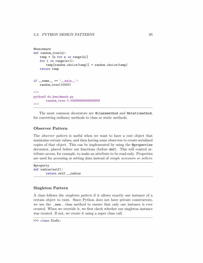
5.3. PYTHON DESIGN PATTERNS 95
@benchmarkdef random_tree(n):
temp = [n for n in range(n)]for i in range(n+1):
temp[random.choice(temp)] = random.choice(temp)return temp
if __name__ == ’__main__’:random_tree(10000)
"""python3 do_benchmark.py
random_tree 0.04999999999999999"""
The most common decorators are @classmethod and @staticmethod,for converting ordinary methods to class or static methods.
Observer Pattern
The observer pattern is useful when we want to have a core object thatmaintains certain values, and then having some observers to create serializedcopies of that object. This can be implemented by using the @propertiesdecorator, placed before our functions (before def). This will control at-tribute access, for example, to make an attribute to be read-only. Propertiesare used for accessing or setting data instead of simple accessors or setters:
@propertydef radius(self):
return self.__radius
Singleton Pattern
A class follows the singleton pattern if it allows exactly one instance of acertain object to exist. Since Python does not have private constructors,we use the new class method to ensure that only one instance is evercreated. When we override it, we first check whether our singleton instancewas created. If not, we create it using a super class call:
>>> class SinEx:
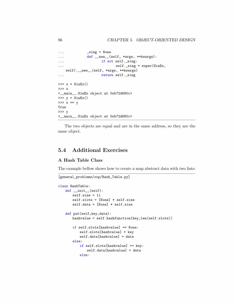
96 CHAPTER 5. OBJECT-ORIENTED DESIGN
... _sing = None
... def __new__(self, *args, **kwargs):
... if not self._sing:
... self._sing = super(SinEx,self).__new__(self, *args, **kwargs)
... return self._sing
>>> x = SinEx()>>> x<__main__.SinEx object at 0xb72d680c>>>> y = SinEx()>>> x == yTrue>>> y<__main__.SinEx object at 0xb72d680c>
The two objects are equal and are in the same address, so they are thesame object.
5.4 Additional Exercises
A Hash Table Class
The example bellow shows how to create a map abstract data with two lists:
[general_problems/oop/Hash_Table.py]
class HashTable:def __init__(self):
self.size = 11self.slots = [None] * self.sizeself.data = [None] * self.size
def put(self,key,data):hashvalue = self.hashfunction(key,len(self.slots))
if self.slots[hashvalue] == None:self.slots[hashvalue] = keyself.data[hashvalue] = data
else:if self.slots[hashvalue] == key:
self.data[hashvalue] = dataelse:
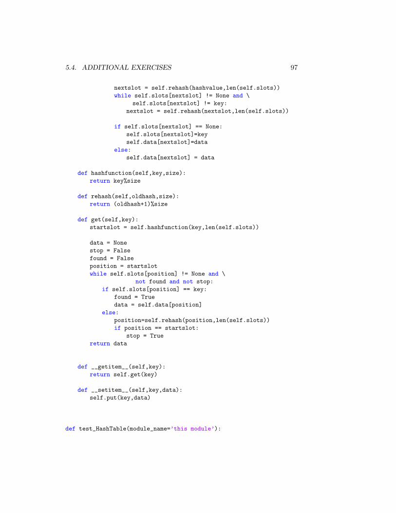
5.4. ADDITIONAL EXERCISES 97
nextslot = self.rehash(hashvalue,len(self.slots))while self.slots[nextslot] != None and \
self.slots[nextslot] != key:nextslot = self.rehash(nextslot,len(self.slots))
if self.slots[nextslot] == None:self.slots[nextslot]=keyself.data[nextslot]=data
else:self.data[nextslot] = data
def hashfunction(self,key,size):return key%size
def rehash(self,oldhash,size):return (oldhash+1)%size
def get(self,key):startslot = self.hashfunction(key,len(self.slots))
data = Nonestop = Falsefound = Falseposition = startslotwhile self.slots[position] != None and \
not found and not stop:if self.slots[position] == key:
found = Truedata = self.data[position]
else:position=self.rehash(position,len(self.slots))if position == startslot:
stop = Truereturn data
def __getitem__(self,key):return self.get(key)
def __setitem__(self,key,data):self.put(key,data)
def test_HashTable(module_name=’this module’):
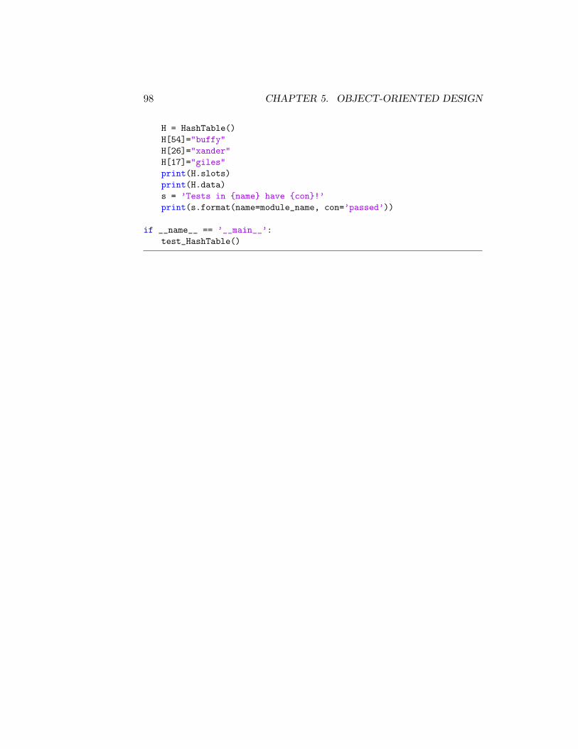
98 CHAPTER 5. OBJECT-ORIENTED DESIGN
H = HashTable()H[54]="buffy"H[26]="xander"H[17]="giles"print(H.slots)print(H.data)s = ’Tests in {name} have {con}!’print(s.format(name=module_name, con=’passed’))
if __name__ == ’__main__’:test_HashTable()
Part II
Algorithms are Fun
99

Chapter 6
Additional Abstract DataStructures
An abstract data type (ADT) is a mathematical model for a certain classof data structures that have similar behavior. Different classes of abstractdata types have many different but functionally equivalent data structuresthat implement them.
Data structures can be classified as either contiguous or linked, depend-ing whether they are based on arrays or pointers. In Python, for instance,contiguously-allocated structures (composed of single slabs of memory) in-clude strings, lists, tuples, and dictionaries. In the following sections we willsee examples of some more specialised continuous structures and examplesof some linked data structures (distinct chunks of memory bound togetherby pointers).
6.1 Stacks
A stack is a linear data structure that can be accessed only at one of itsends (which we will refers as the top) for either storing or retrieving. Inother words, array access of elements in a stack is restricted and they arean example of a last-in-first-out (LIFO) structure. You can think of a stackas a huge pile of books on your desk. Stacks need to have the followingoperations running at O(1):
push Insert an item at the top of the stack.
pop Remove an item from the top of the stack.
101
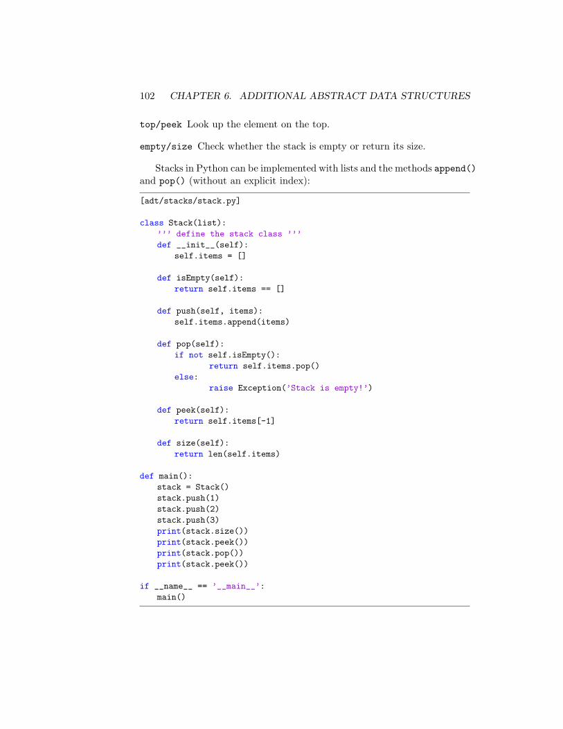
102 CHAPTER 6. ADDITIONAL ABSTRACT DATA STRUCTURES
top/peek Look up the element on the top.
empty/size Check whether the stack is empty or return its size.
Stacks in Python can be implemented with lists and the methods append()and pop() (without an explicit index):
[adt/stacks/stack.py]
class Stack(list):’’’ define the stack class ’’’def __init__(self):
self.items = []
def isEmpty(self):return self.items == []
def push(self, items):self.items.append(items)
def pop(self):if not self.isEmpty():
return self.items.pop()else:
raise Exception(’Stack is empty!’)
def peek(self):return self.items[-1]
def size(self):return len(self.items)
def main():stack = Stack()stack.push(1)stack.push(2)stack.push(3)print(stack.size())print(stack.peek())print(stack.pop())print(stack.peek())
if __name__ == ’__main__’:main()
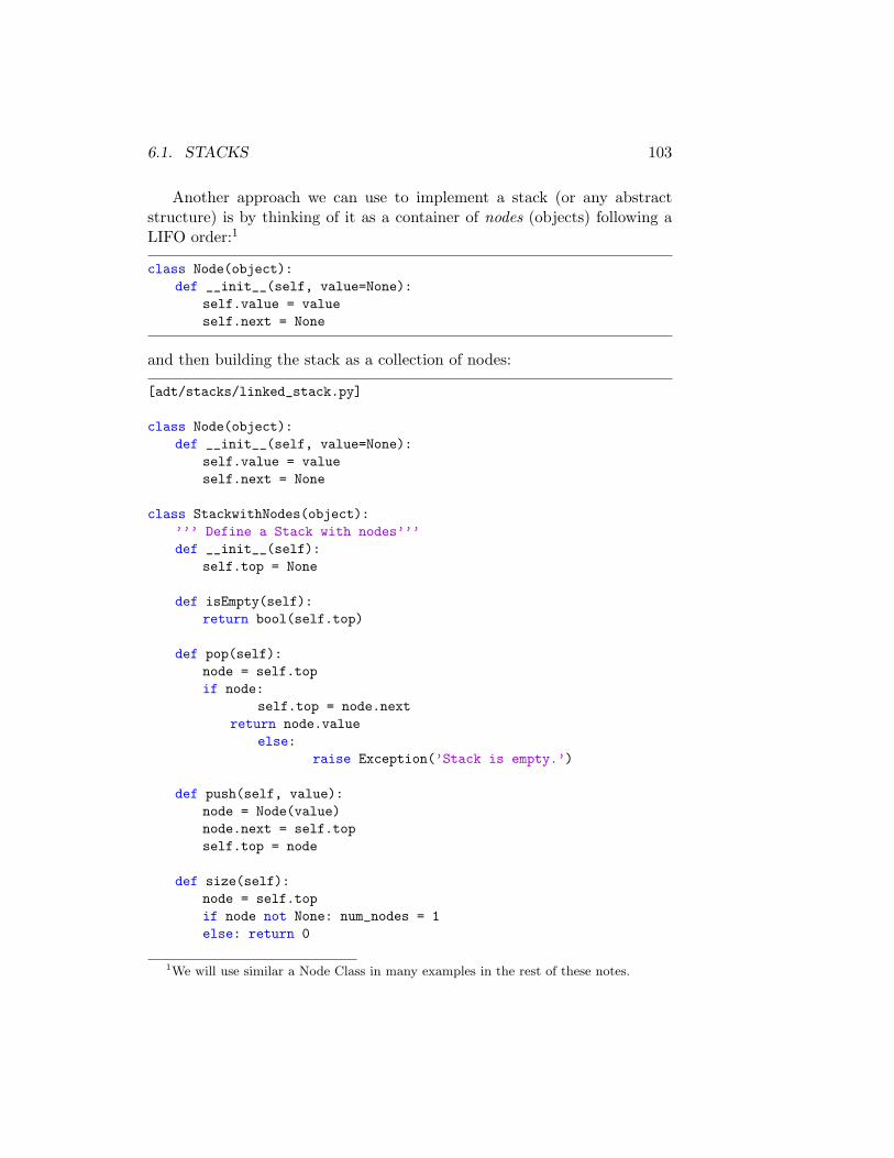
6.1. STACKS 103
Another approach we can use to implement a stack (or any abstractstructure) is by thinking of it as a container of nodes (objects) following aLIFO order:1
class Node(object):def __init__(self, value=None):
self.value = valueself.next = None
and then building the stack as a collection of nodes:
[adt/stacks/linked_stack.py]
class Node(object):def __init__(self, value=None):
self.value = valueself.next = None
class StackwithNodes(object):’’’ Define a Stack with nodes’’’def __init__(self):
self.top = None
def isEmpty(self):return bool(self.top)
def pop(self):node = self.topif node:
self.top = node.nextreturn node.value
else:raise Exception(’Stack is empty.’)
def push(self, value):node = Node(value)node.next = self.topself.top = node
def size(self):node = self.topif node not None: num_nodes = 1else: return 0
1We will use similar a Node Class in many examples in the rest of these notes.
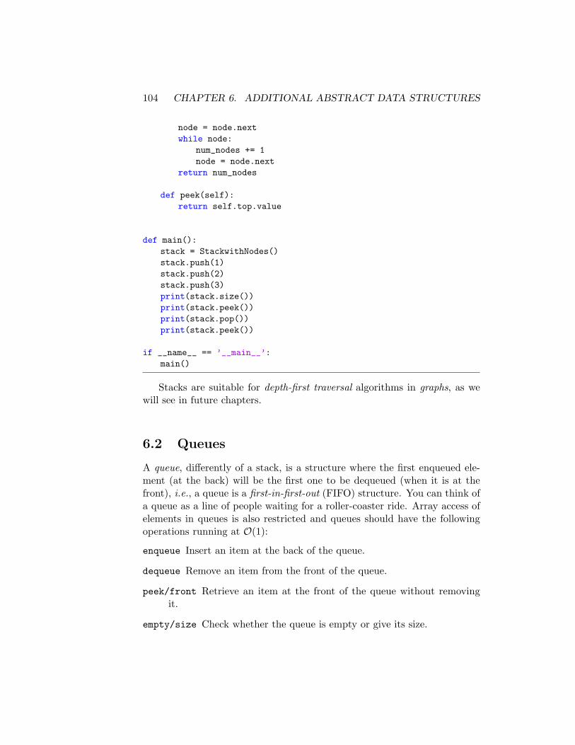
104 CHAPTER 6. ADDITIONAL ABSTRACT DATA STRUCTURES
node = node.nextwhile node:
num_nodes += 1node = node.next
return num_nodes
def peek(self):return self.top.value
def main():stack = StackwithNodes()stack.push(1)stack.push(2)stack.push(3)print(stack.size())print(stack.peek())print(stack.pop())print(stack.peek())
if __name__ == ’__main__’:main()
Stacks are suitable for depth-first traversal algorithms in graphs, as wewill see in future chapters.
6.2 Queues
A queue, differently of a stack, is a structure where the first enqueued ele-ment (at the back) will be the first one to be dequeued (when it is at thefront), i.e., a queue is a first-in-first-out (FIFO) structure. You can think ofa queue as a line of people waiting for a roller-coaster ride. Array access ofelements in queues is also restricted and queues should have the followingoperations running at O(1):
enqueue Insert an item at the back of the queue.
dequeue Remove an item from the front of the queue.
peek/front Retrieve an item at the front of the queue without removingit.
empty/size Check whether the queue is empty or give its size.
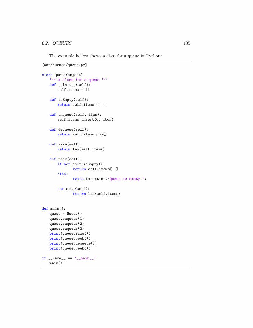
6.2. QUEUES 105
The example bellow shows a class for a queue in Python:
[adt/queues/queue.py]
class Queue(object):’’’ a class for a queue ’’’def __init__(self):
self.items = []
def isEmpty(self):return self.items == []
def enqueue(self, item):self.items.insert(0, item)
def dequeue(self):return self.items.pop()
def size(self):return len(self.items)
def peek(self):if not self.isEmpty():
return self.items[-1]else:
raise Exception(’Queue is empty.’)
def size(self):return len(self.items)
def main():queue = Queue()queue.enqueue(1)queue.enqueue(2)queue.enqueue(3)print(queue.size())print(queue.peek())print(queue.dequeue())print(queue.peek())
if __name__ == ’__main__’:main()
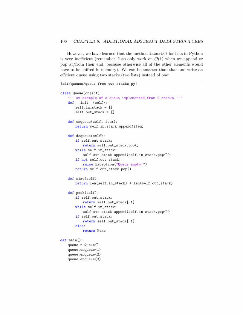
106 CHAPTER 6. ADDITIONAL ABSTRACT DATA STRUCTURES
However, we have learned that the method insert() for lists in Pythonis very inefficient (remember, lists only work on O(1) when we append orpop at/from their end, because otherwise all of the other elements wouldhave to be shifted in memory). We can be smarter than that and write anefficient queue using two stacks (two lists) instead of one:
[adt/queues/queue_from_two_stacks.py]
class Queue(object):’’’ an example of a queue implemented from 2 stacks ’’’def __init__(self):
self.in_stack = []self.out_stack = []
def enqueue(self, item):return self.in_stack.append(item)
def dequeue(self):if self.out_stack:
return self.out_stack.pop()while self.in_stack:
self.out_stack.append(self.in_stack.pop())if not self.out_stack:
raise Exception("Queue empty!")return self.out_stack.pop()
def size(self):return len(self.in_stack) + len(self.out_stack)
def peek(self):if self.out_stack:
return self.out_stack[-1]while self.in_stack:
self.out_stack.append(self.in_stack.pop())if self.out_stack:
return self.out_stack[-1]else:
return None
def main():queue = Queue()queue.enqueue(1)queue.enqueue(2)queue.enqueue(3)
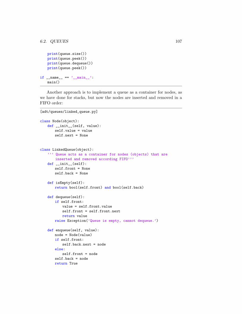
6.2. QUEUES 107
print(queue.size())print(queue.peek())print(queue.dequeue())print(queue.peek())
if __name__ == ’__main__’:main()
Another approach is to implement a queue as a container for nodes, aswe have done for stacks, but now the nodes are inserted and removed in aFIFO order:
[adt/queues/linked_queue.py]
class Node(object):def __init__(self, value):
self.value = valueself.next = None
class LinkedQueue(object):’’’ Queue acts as a container for nodes (objects) that are
inserted and removed according FIFO’’’def __init__(self):
self.front = Noneself.back = None
def isEmpty(self):return bool(self.front) and bool(self.back)
def dequeue(self):if self.front:
value = self.front.valueself.front = self.front.nextreturn value
raise Exception(’Queue is empty, cannot dequeue.’)
def enqueue(self, value):node = Node(value)if self.front:
self.back.next = nodeelse:
self.front = nodeself.back = nodereturn True
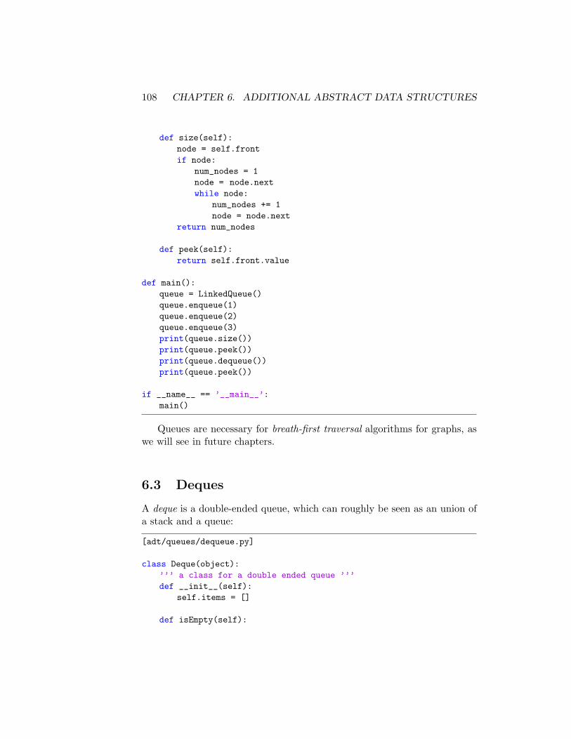
108 CHAPTER 6. ADDITIONAL ABSTRACT DATA STRUCTURES
def size(self):node = self.frontif node:
num_nodes = 1node = node.nextwhile node:
num_nodes += 1node = node.next
return num_nodes
def peek(self):return self.front.value
def main():queue = LinkedQueue()queue.enqueue(1)queue.enqueue(2)queue.enqueue(3)print(queue.size())print(queue.peek())print(queue.dequeue())print(queue.peek())
if __name__ == ’__main__’:main()
Queues are necessary for breath-first traversal algorithms for graphs, aswe will see in future chapters.
6.3 Deques
A deque is a double-ended queue, which can roughly be seen as an union ofa stack and a queue:
[adt/queues/dequeue.py]
class Deque(object):’’’ a class for a double ended queue ’’’def __init__(self):
self.items = []
def isEmpty(self):
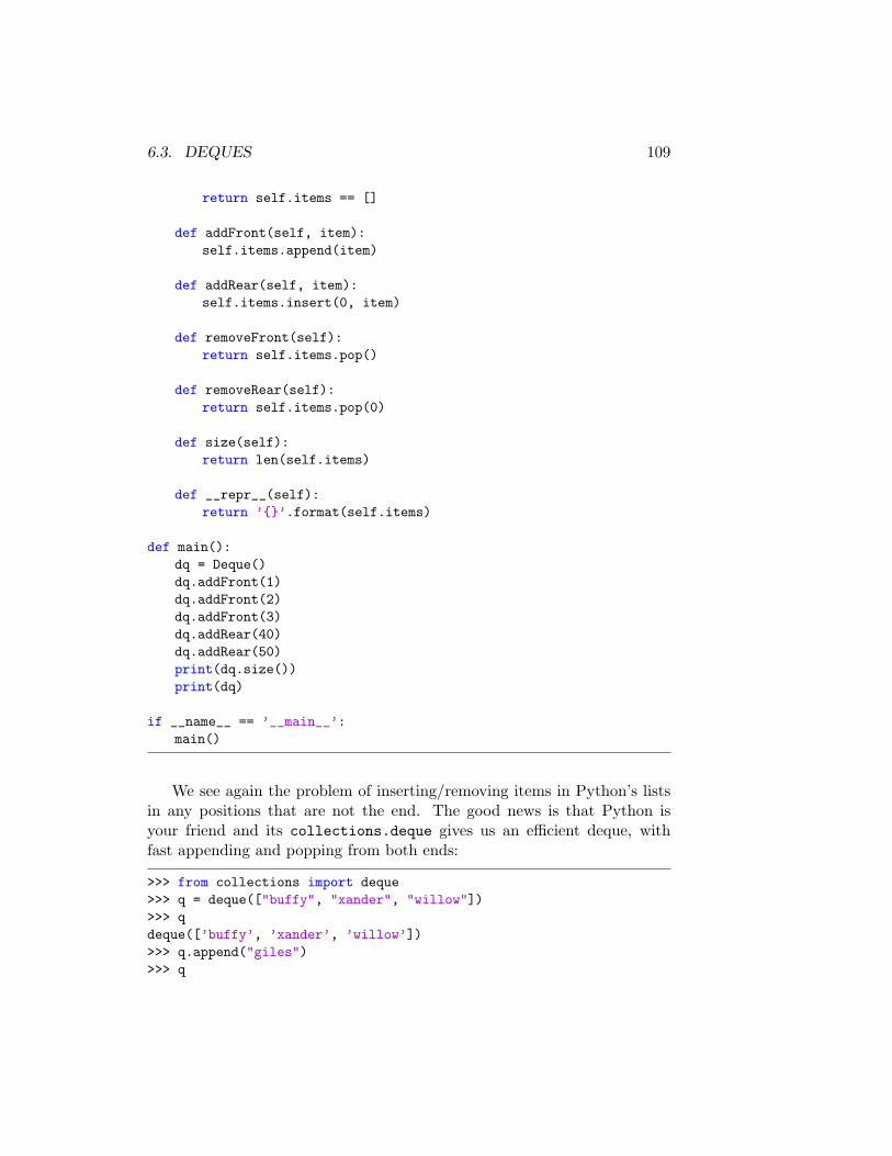
6.3. DEQUES 109
return self.items == []
def addFront(self, item):self.items.append(item)
def addRear(self, item):self.items.insert(0, item)
def removeFront(self):return self.items.pop()
def removeRear(self):return self.items.pop(0)
def size(self):return len(self.items)
def __repr__(self):return ’{}’.format(self.items)
def main():dq = Deque()dq.addFront(1)dq.addFront(2)dq.addFront(3)dq.addRear(40)dq.addRear(50)print(dq.size())print(dq)
if __name__ == ’__main__’:main()
We see again the problem of inserting/removing items in Python’s listsin any positions that are not the end. The good news is that Python isyour friend and its collections.deque gives us an efficient deque, withfast appending and popping from both ends:
>>> from collections import deque>>> q = deque(["buffy", "xander", "willow"])>>> qdeque([’buffy’, ’xander’, ’willow’])>>> q.append("giles")>>> q
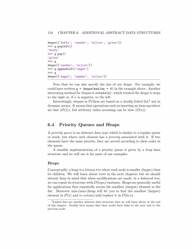
110 CHAPTER 6. ADDITIONAL ABSTRACT DATA STRUCTURES
deque([’buffy’, ’xander’, ’willow’, ’giles’])>>> q.popleft()’buffy’>>> q.pop()’giles’>>> qdeque([’xander’, ’willow’])>>> q.appendleft(’angel’)>>> qdeque([’angel’, ’xander’, ’willow’])
Note that we can also specify the size of our deque. For example, wecould have written q = deque(maxlen = 4) in the example above. Anotherinteresting method for deques is rotate(n), which rotated the deque n stepsto the right or, if n is negative, to the left.
Interestingly, deques in Python are based on a doubly linked list,2 not indynamic arrays. It means that operations such as inserting an item anywhereare fast (O(1)), but arbitrary index accessing can be slow (O(n)).
6.4 Priority Queues and Heaps
A priority queue is an abstract data type which is similar to a regular queueor stack, but where each element has a priority associated with it. If twoelements have the same priority, they are served according to their order inthe queue.
A sensible implementation of a priority queue is given by a heap datastructure and we will use it for most of our examples.
Heaps
Conceptually, a heap is a binary tree where each node is smaller (larger) thanits children. We will learn about trees in the next chapters but we shouldalready keep in mind that when modifications are made, in a balanced tree,we can repair its structure withO(logn) runtimes. Heaps are generally usefulfor applications that repeatedly access the smallest (largest) element in thelist. Moreover min-(max-)heap will let you to find the smallest (largest)element in O(1) and to extract/add/replace it in O(ln n).
2Linked lists are another abstract data structure that we will learn about at the endof this chapter. Doubly here means that their nodes have links to the next and to theprevious node.
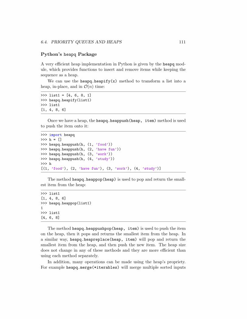
6.4. PRIORITY QUEUES AND HEAPS 111
Python’s heapq Package
A very efficient heap implementation in Python is given by the heapq mod-ule, which provides functions to insert and remove items while keeping thesequence as a heap.
We can use the heapq.heapify(x) method to transform a list into aheap, in-place, and in O(n) time:
>>> list1 = [4, 6, 8, 1]>>> heapq.heapify(list1)>>> list1[1, 4, 8, 6]
Once we have a heap, the heapq.heappush(heap, item) method is usedto push the item onto it:
>>> import heapq>>> h = []>>> heapq.heappush(h, (1, ’food’))>>> heapq.heappush(h, (2, ’have fun’))>>> heapq.heappush(h, (3, ’work’))>>> heapq.heappush(h, (4, ’study’))>>> h[(1, ’food’), (2, ’have fun’), (3, ’work’), (4, ’study’)]
The method heapq.heappop(heap) is used to pop and return the small-est item from the heap:
>>> list1[1, 4, 8, 6]>>> heapq.heappop(list1)1>>> list1[4, 6, 8]
The method heapq.heappushpop(heap, item) is used to push the itemon the heap, then it pops and returns the smallest item from the heap. Ina similar way, heapq.heapreplace(heap, item) will pop and return thesmallest item from the heap, and then push the new item. The heap sizedoes not change in any of these methods and they are more efficient thanusing each method separately.
In addition, many operations can be made using the heap’s propriety.For example heapq.merge(*iterables) will merge multiple sorted inputs
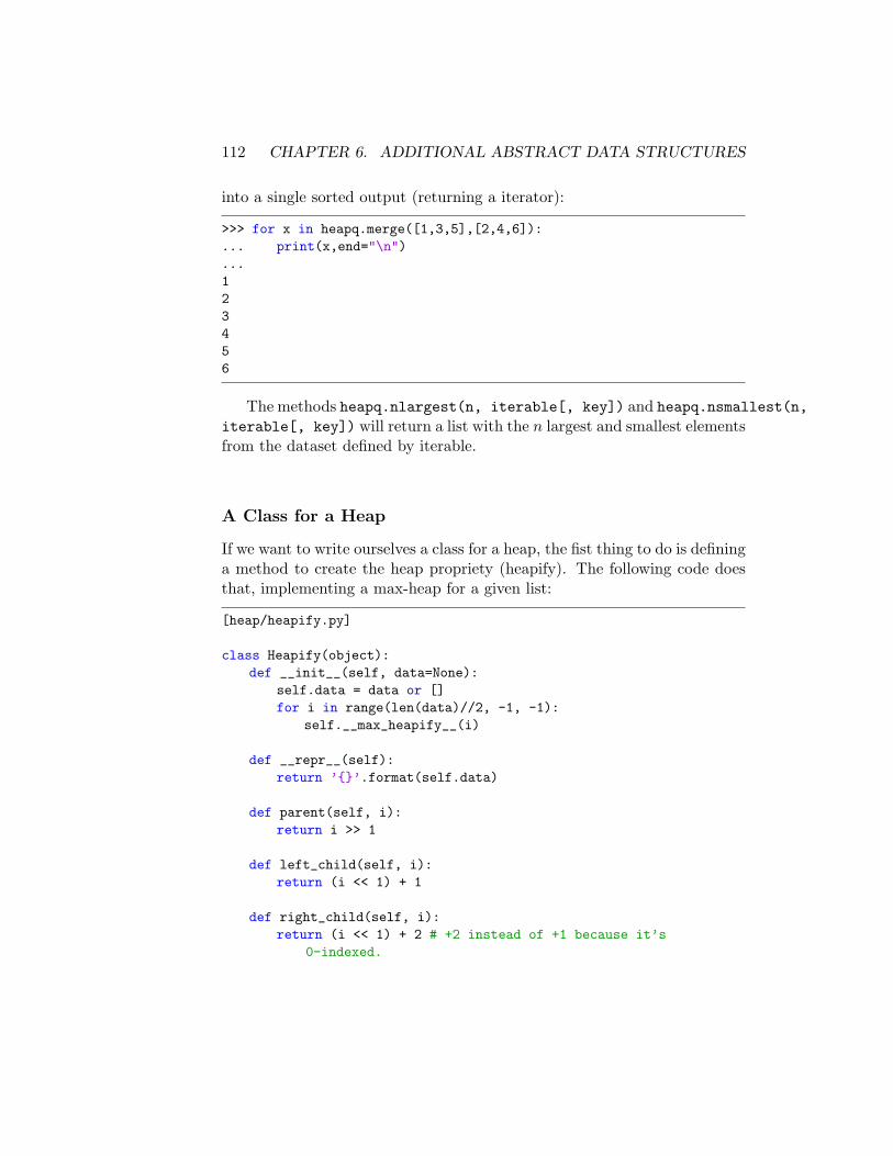
112 CHAPTER 6. ADDITIONAL ABSTRACT DATA STRUCTURES
into a single sorted output (returning a iterator):
>>> for x in heapq.merge([1,3,5],[2,4,6]):... print(x,end="\n")...123456
The methods heapq.nlargest(n, iterable[, key]) and heapq.nsmallest(n,iterable[, key]) will return a list with the n largest and smallest elementsfrom the dataset defined by iterable.
A Class for a Heap
If we want to write ourselves a class for a heap, the fist thing to do is defininga method to create the heap propriety (heapify). The following code doesthat, implementing a max-heap for a given list:
[heap/heapify.py]
class Heapify(object):def __init__(self, data=None):
self.data = data or []for i in range(len(data)//2, -1, -1):
self.__max_heapify__(i)
def __repr__(self):return ’{}’.format(self.data)
def parent(self, i):return i >> 1
def left_child(self, i):return (i << 1) + 1
def right_child(self, i):return (i << 1) + 2 # +2 instead of +1 because it’s
0-indexed.
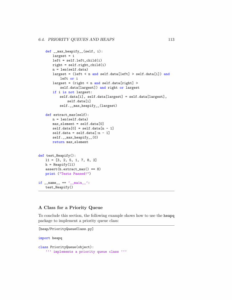
6.4. PRIORITY QUEUES AND HEAPS 113
def __max_heapify__(self, i):largest = ileft = self.left_child(i)right = self.right_child(i)n = len(self.data)largest = (left < n and self.data[left] > self.data[i]) and
left or ilargest = (right < n and self.data[right] >
self.data[largest]) and right or largestif i is not largest:
self.data[i], self.data[largest] = self.data[largest],self.data[i]
self.__max_heapify__(largest)
def extract_max(self):n = len(self.data)max_element = self.data[0]self.data[0] = self.data[n - 1]self.data = self.data[:n - 1]self.__max_heapify__(0)return max_element
def test_Heapify():l1 = [3, 2, 5, 1, 7, 8, 2]h = Heapify(l1)assert(h.extract_max() == 8)print ("Tests Passed!")
if __name__ == ’__main__’:test_Heapify()
A Class for a Priority Queue
To conclude this section, the following example shows how to use the heapqpackage to implement a priority queue class:
[heap/PriorityQueueClass.py]
import heapq
class PriorityQueue(object):’’’ implements a priority queue class ’’’
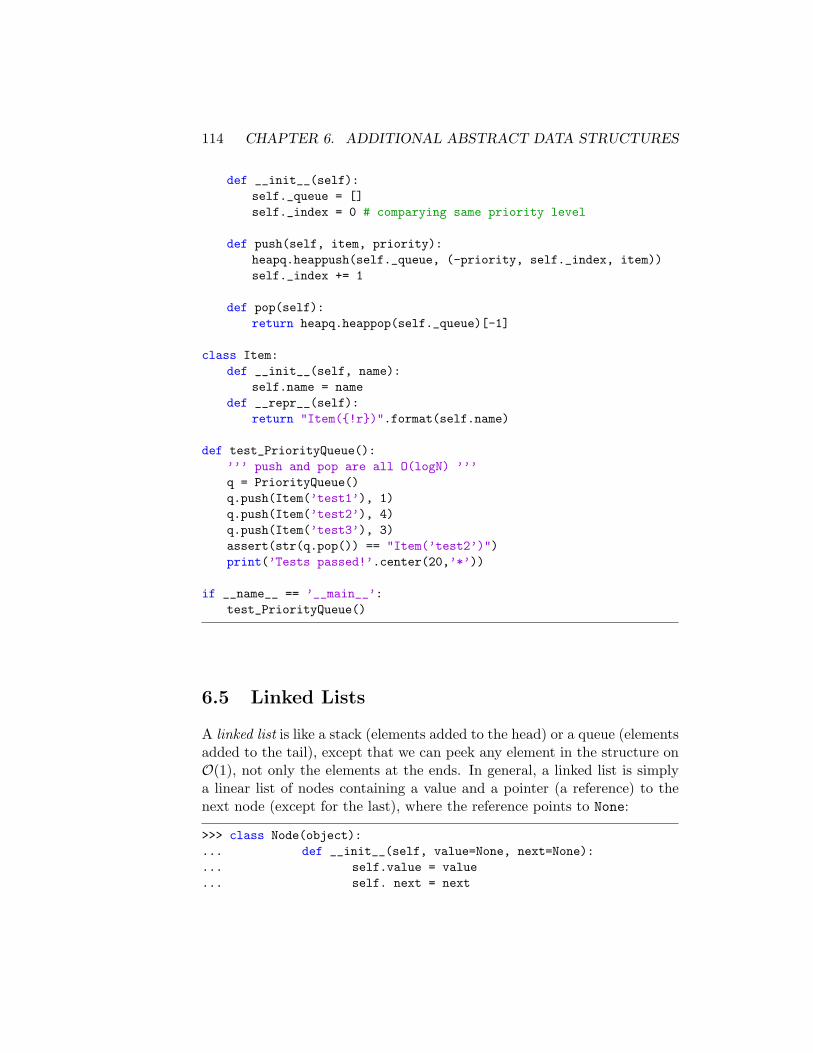
114 CHAPTER 6. ADDITIONAL ABSTRACT DATA STRUCTURES
def __init__(self):self._queue = []self._index = 0 # comparying same priority level
def push(self, item, priority):heapq.heappush(self._queue, (-priority, self._index, item))self._index += 1
def pop(self):return heapq.heappop(self._queue)[-1]
class Item:def __init__(self, name):
self.name = namedef __repr__(self):
return "Item({!r})".format(self.name)
def test_PriorityQueue():’’’ push and pop are all O(logN) ’’’q = PriorityQueue()q.push(Item(’test1’), 1)q.push(Item(’test2’), 4)q.push(Item(’test3’), 3)assert(str(q.pop()) == "Item(’test2’)")print(’Tests passed!’.center(20,’*’))
if __name__ == ’__main__’:test_PriorityQueue()
6.5 Linked Lists
A linked list is like a stack (elements added to the head) or a queue (elementsadded to the tail), except that we can peek any element in the structure onO(1), not only the elements at the ends. In general, a linked list is simplya linear list of nodes containing a value and a pointer (a reference) to thenext node (except for the last), where the reference points to None:
>>> class Node(object):... def __init__(self, value=None, next=None):... self.value = value... self. next = next
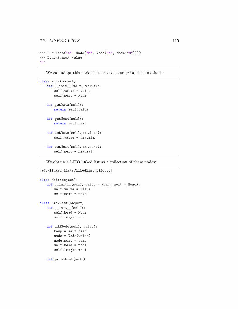
6.5. LINKED LISTS 115
>>> L = Node("a", Node("b", Node("c", Node("d"))))>>> L.next.next.value’c’
We can adapt this node class accept some get and set methods:
class Node(object):def __init__(self, value):
self.value = valueself.next = None
def getData(self):return self.value
def getNext(self):return self.next
def setData(self, newdata):self.value = newdata
def setNext(self, newnext):self.next = newnext
We obtain a LIFO linked list as a collection of these nodes:
[adt/linked_lists/likedlist_lifo.py]
class Node(object):def __init__(self, value = None, next = None):
self.value = valueself.next = next
class LinkList(object):def __init__(self):
self.head = Noneself.lenght = 0
def addNode(self, value):temp = self.headnode = Node(value)node.next = tempself.head = nodeself.lenght += 1
def printList(self):
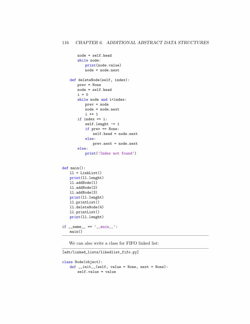
116 CHAPTER 6. ADDITIONAL ABSTRACT DATA STRUCTURES
node = self.headwhile node:
print(node.value)node = node.next
def deleteNode(self, index):prev = Nonenode = self.headi = 0while node and i<index:
prev = nodenode = node.nexti += 1
if index == i:self.lenght -= 1if prev == None:
self.head = node.nextelse:
prev.next = node.nextelse:
print(’Index not found’)
def main():ll = LinkList()print(ll.lenght)ll.addNode(1)ll.addNode(2)ll.addNode(3)print(ll.lenght)ll.printList()ll.deleteNode(4)ll.printList()print(ll.lenght)
if __name__ == ’__main__’:main()
We can also write a class for FIFO linked list:
[adt/linked_lists/likedlist_fifo.py]
class Node(object):def __init__(self, value = None, next = None):
self.value = value
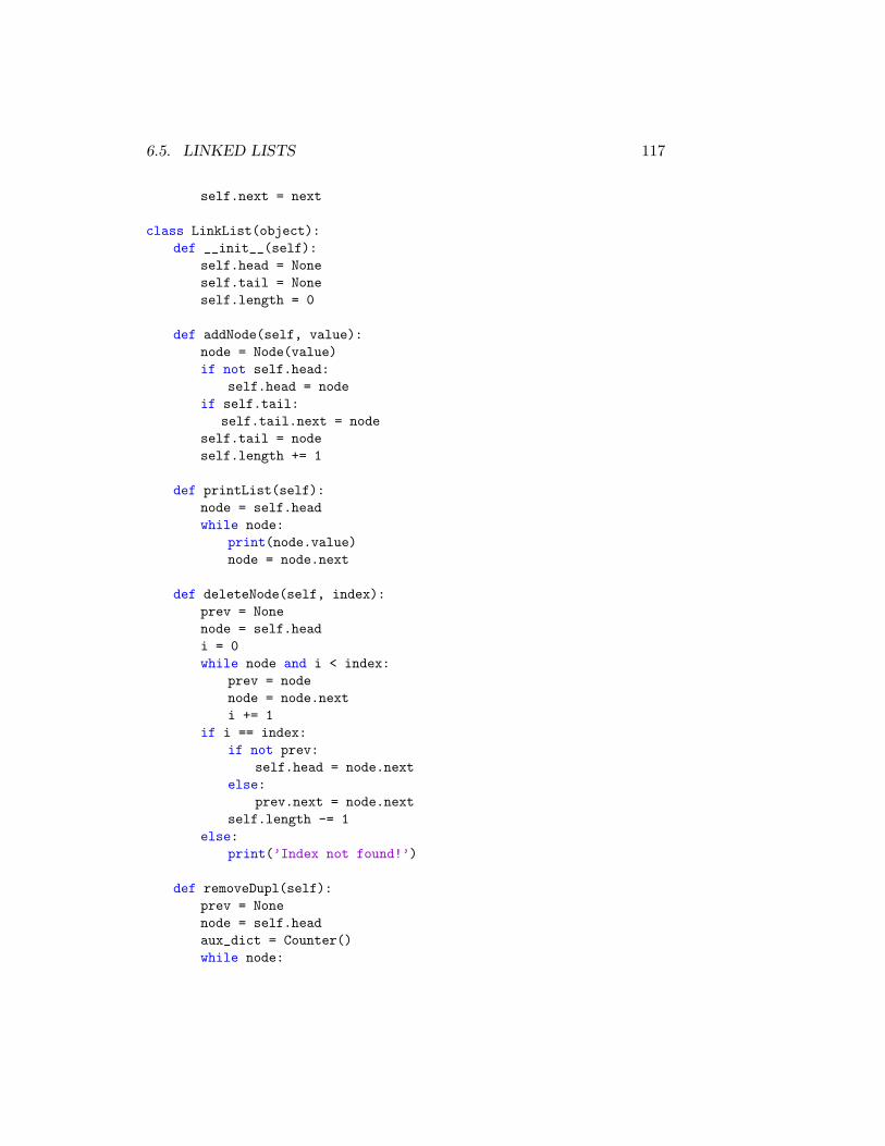
6.5. LINKED LISTS 117
self.next = next
class LinkList(object):def __init__(self):
self.head = Noneself.tail = Noneself.length = 0
def addNode(self, value):node = Node(value)if not self.head:
self.head = nodeif self.tail:
self.tail.next = nodeself.tail = nodeself.length += 1
def printList(self):node = self.headwhile node:
print(node.value)node = node.next
def deleteNode(self, index):prev = Nonenode = self.headi = 0while node and i < index:
prev = nodenode = node.nexti += 1
if i == index:if not prev:
self.head = node.nextelse:
prev.next = node.nextself.length -= 1
else:print(’Index not found!’)
def removeDupl(self):prev = Nonenode = self.headaux_dict = Counter()while node:
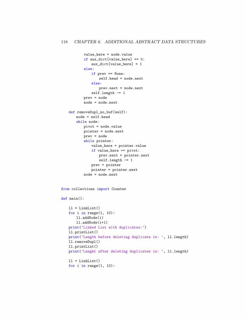
118 CHAPTER 6. ADDITIONAL ABSTRACT DATA STRUCTURES
value_here = node.valueif aux_dict[value_here] == 0:
aux_dict[value_here] = 1else:
if prev == None:self.head = node.next
else:prev.next = node.next
self.length -= 1prev = nodenode = node.next
def removeDupl_no_buf(self):node = self.headwhile node:
pivot = node.valuepointer = node.nextprev = nodewhile pointer:
value_here = pointer.valueif value_here == pivot:
prev.next = pointer.nextself.length -= 1
prev = pointerpointer = pointer.next
node = node.next
from collections import Counter
def main():
ll = LinkList()for i in range(1, 10):
ll.addNode(i)ll.addNode(i+1)
print(’Linked List with duplicates:’)ll.printList()print(’Length before deleting duplicate is: ’, ll.length)ll.removeDupl()ll.printList()print(’Lenght after deleting duplicates is: ’, ll.length)
ll = LinkList()for i in range(1, 10):
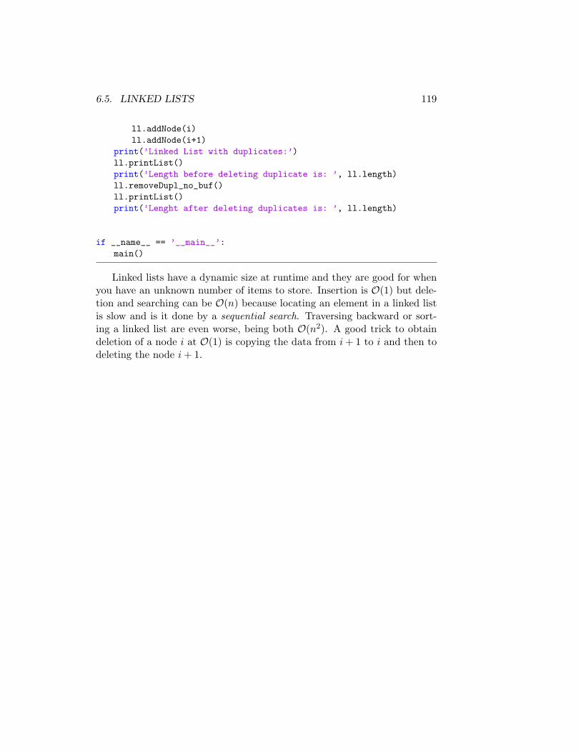
6.5. LINKED LISTS 119
ll.addNode(i)ll.addNode(i+1)
print(’Linked List with duplicates:’)ll.printList()print(’Length before deleting duplicate is: ’, ll.length)ll.removeDupl_no_buf()ll.printList()print(’Lenght after deleting duplicates is: ’, ll.length)
if __name__ == ’__main__’:main()
Linked lists have a dynamic size at runtime and they are good for whenyou have an unknown number of items to store. Insertion is O(1) but dele-tion and searching can be O(n) because locating an element in a linked listis slow and is it done by a sequential search. Traversing backward or sort-ing a linked list are even worse, being both O(n2). A good trick to obtaindeletion of a node i at O(1) is copying the data from i + 1 to i and then todeleting the node i + 1.
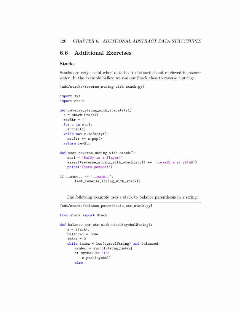
120 CHAPTER 6. ADDITIONAL ABSTRACT DATA STRUCTURES
6.6 Additional Exercises
Stacks
Stacks are very useful when data has to be sorted and retrieved in reverseorder. In the example bellow we use our Stack class to reverse a string:
[adt/stacks/reverse_string_with_stack.py]
import sysimport stack
def reverse_string_with_stack(str1):s = stack.Stack()revStr = ’’for c in str1:s.push(c)
while not s.isEmpty():revStr += s.pop()
return revStr
def test_reverse_string_with_stack():str1 = ’Buffy is a Slayer!’assert(reverse_string_with_stack(str1) == ’!reyalS a si yffuB’)print(’Tests passed!’)
if __name__ == ’__main__’:test_reverse_string_with_stack()
The following example uses a stack to balance parenthesis in a string:
[adt/stacks/balance_parenthesis_str_stack.py]
from stack import Stack
def balance_par_str_with_stack(symbolString):s = Stack()balanced = Trueindex = 0while index < len(symbolString) and balanced:
symbol = symbolString[index]if symbol == "(":
s.push(symbol)else:
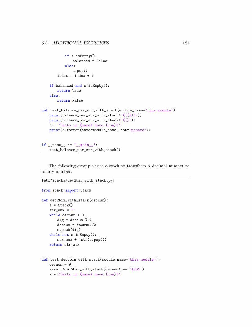
6.6. ADDITIONAL EXERCISES 121
if s.isEmpty():balanced = False
else:s.pop()
index = index + 1
if balanced and s.isEmpty():return True
else:return False
def test_balance_par_str_with_stack(module_name=’this module’):print(balance_par_str_with_stack(’((()))’))print(balance_par_str_with_stack(’(()’))s = ’Tests in {name} have {con}!’print(s.format(name=module_name, con=’passed’))
if __name__ == ’__main__’:test_balance_par_str_with_stack()
The following example uses a stack to transform a decimal number tobinary number:
[atf/stacks/dec2bin_with_stack.py]
from stack import Stack
def dec2bin_with_stack(decnum):s = Stack()str_aux = ’’while decnum > 0:
dig = decnum % 2decnum = decnum//2s.push(dig)
while not s.isEmpty():str_aux += str(s.pop())
return str_aux
def test_dec2bin_with_stack(module_name=’this module’):decnum = 9assert(dec2bin_with_stack(decnum) == ’1001’)s = ’Tests in {name} have {con}!’
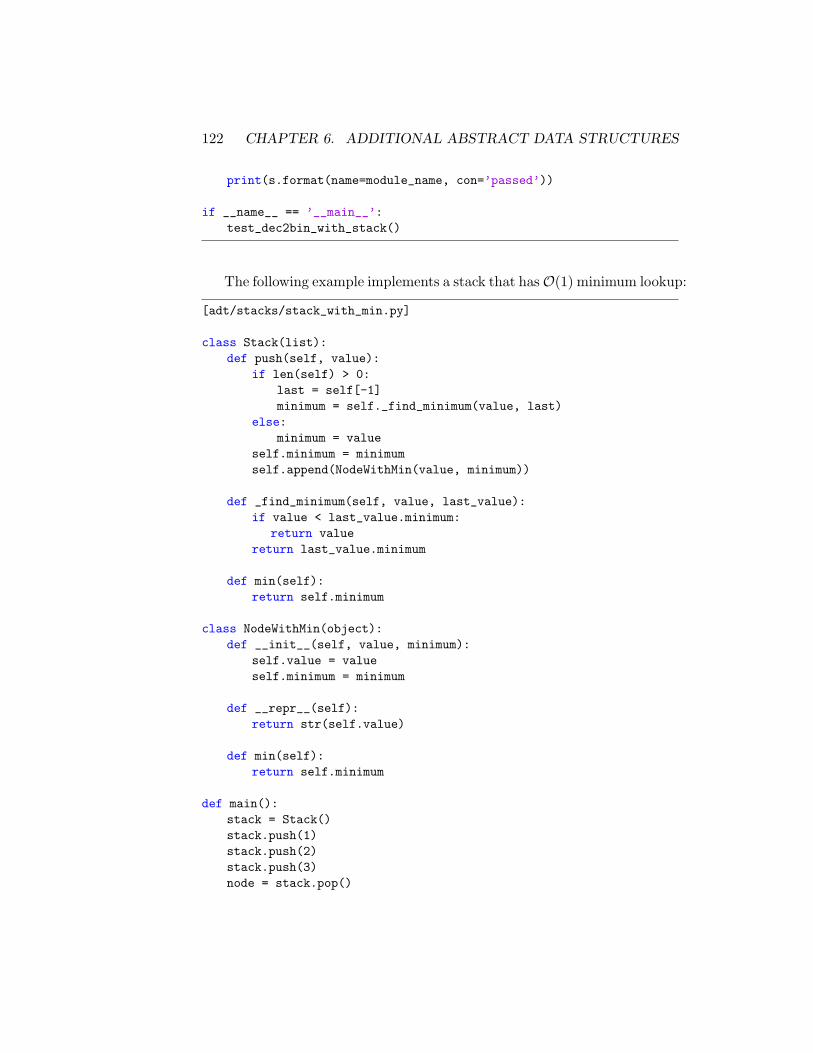
122 CHAPTER 6. ADDITIONAL ABSTRACT DATA STRUCTURES
print(s.format(name=module_name, con=’passed’))
if __name__ == ’__main__’:test_dec2bin_with_stack()
The following example implements a stack that hasO(1) minimum lookup:
[adt/stacks/stack_with_min.py]
class Stack(list):def push(self, value):
if len(self) > 0:last = self[-1]minimum = self._find_minimum(value, last)
else:minimum = value
self.minimum = minimumself.append(NodeWithMin(value, minimum))
def _find_minimum(self, value, last_value):if value < last_value.minimum:
return valuereturn last_value.minimum
def min(self):return self.minimum
class NodeWithMin(object):def __init__(self, value, minimum):
self.value = valueself.minimum = minimum
def __repr__(self):return str(self.value)
def min(self):return self.minimum
def main():stack = Stack()stack.push(1)stack.push(2)stack.push(3)node = stack.pop()
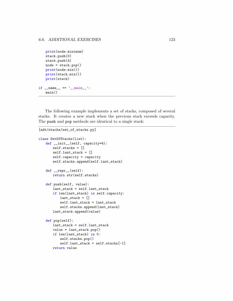
6.6. ADDITIONAL EXERCISES 123
print(node.minimum)stack.push(0)stack.push(4)node = stack.pop()print(node.min())print(stack.min())print(stack)
if __name__ == ’__main__’:main()
The following example implements a set of stacks, composed of severalstacks. It creates a new stack when the previous stack exceeds capacity.The push and pop methods are identical to a single stack:
[adt/stacks/set_of_stacks.py]
class SetOfStacks(list):def __init__(self, capacity=4):
self.stacks = []self.last_stack = []self.capacity = capacityself.stacks.append(self.last_stack)
def __repr__(self):return str(self.stacks)
def push(self, value):last_stack = self.last_stackif len(last_stack) is self.capacity:
last_stack = []self.last_stack = last_stackself.stacks.append(last_stack)
last_stack.append(value)
def pop(self):last_stack = self.last_stackvalue = last_stack.pop()if len(last_stack) is 0:
self.stacks.pop()self.last_stack = self.stacks[-1]
return value
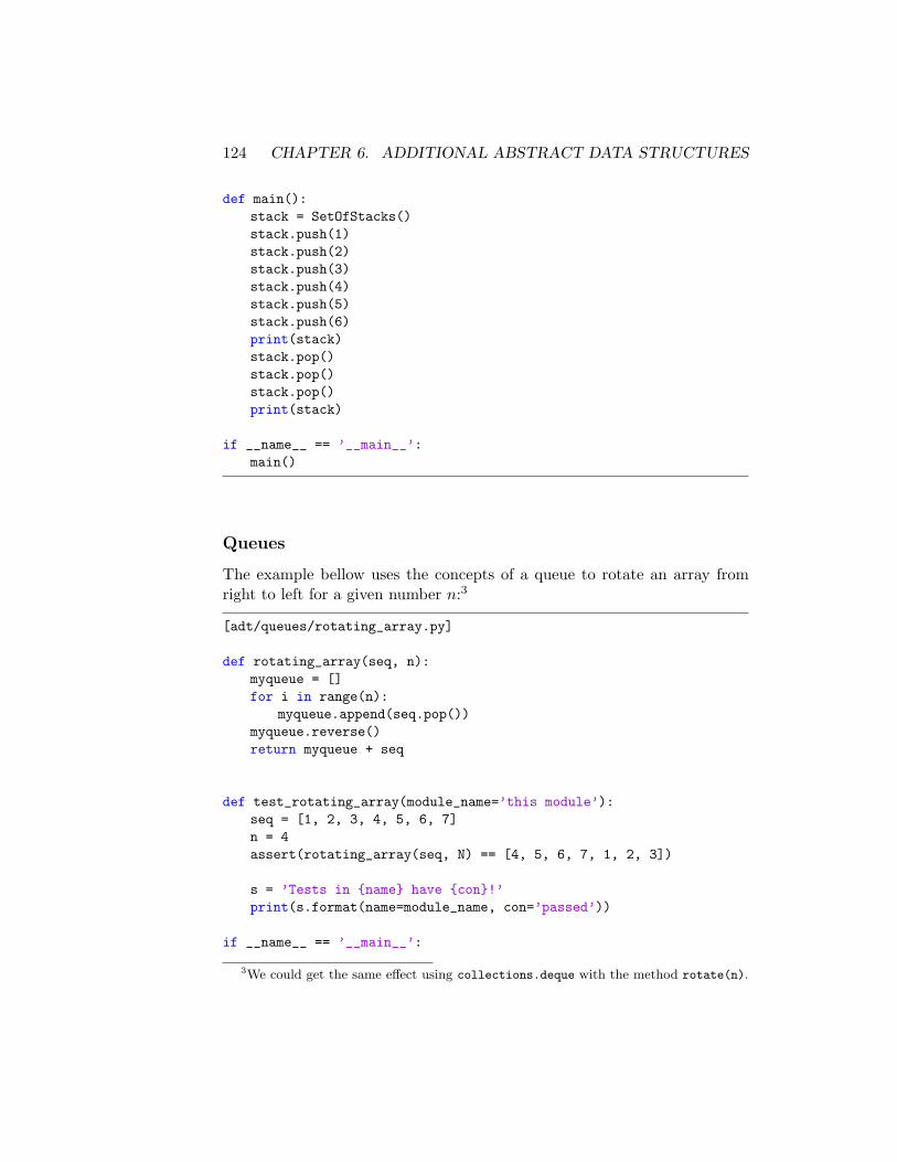
124 CHAPTER 6. ADDITIONAL ABSTRACT DATA STRUCTURES
def main():stack = SetOfStacks()stack.push(1)stack.push(2)stack.push(3)stack.push(4)stack.push(5)stack.push(6)print(stack)stack.pop()stack.pop()stack.pop()print(stack)
if __name__ == ’__main__’:main()
Queues
The example bellow uses the concepts of a queue to rotate an array fromright to left for a given number n:3
[adt/queues/rotating_array.py]
def rotating_array(seq, n):myqueue = []for i in range(n):
myqueue.append(seq.pop())myqueue.reverse()return myqueue + seq
def test_rotating_array(module_name=’this module’):seq = [1, 2, 3, 4, 5, 6, 7]n = 4assert(rotating_array(seq, N) == [4, 5, 6, 7, 1, 2, 3])
s = ’Tests in {name} have {con}!’print(s.format(name=module_name, con=’passed’))
if __name__ == ’__main__’:
3We could get the same effect using collections.deque with the method rotate(n).
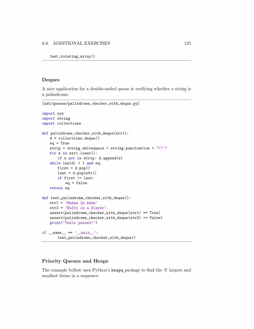
6.6. ADDITIONAL EXERCISES 125
test_rotating_array()
Deques
A nice application for a double-ended queue is verifying whether a string isa palindrome:
[adt/queues/palindrome_checker_with_deque.py]
import sysimport stringimport collections
def palindrome_checker_with_deque(str1):d = collections.deque()eq = Truestrip = string.whitespace + string.punctuation + "\"’"for s in str1.lower():
if s not in strip: d.append(s)while len(d) > 1 and eq:
first = d.pop()last = d.popleft()if first != last:
eq = Falsereturn eq
def test_palindrome_checker_with_deque():str1 = ’Madam Im Adam’str2 = ’Buffy is a Slayer’assert(palindrome_checker_with_deque(str1) == True)assert(palindrome_checker_with_deque(str2) == False)print(’Tests passed!’)
if __name__ == ’__main__’:test_palindrome_checker_with_deque()
Priority Queues and Heaps
The example bellow uses Python’s heapq package to find the N largest andsmallest items in a sequence:
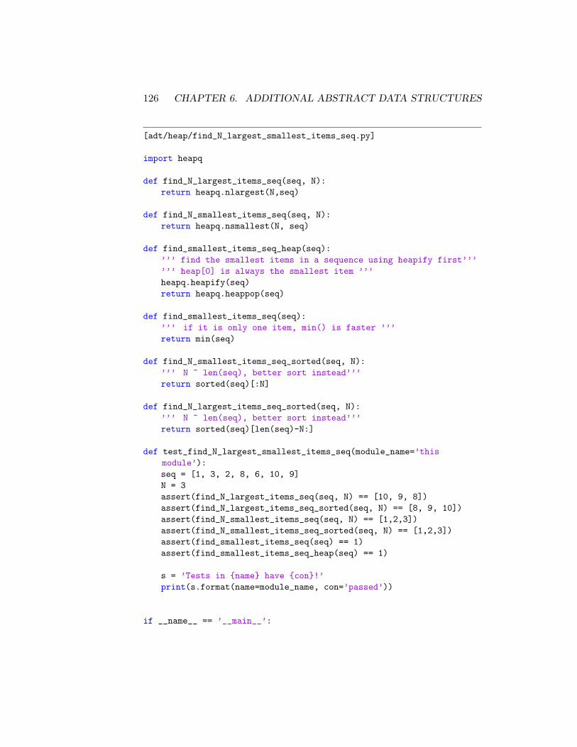
126 CHAPTER 6. ADDITIONAL ABSTRACT DATA STRUCTURES
[adt/heap/find_N_largest_smallest_items_seq.py]
import heapq
def find_N_largest_items_seq(seq, N):return heapq.nlargest(N,seq)
def find_N_smallest_items_seq(seq, N):return heapq.nsmallest(N, seq)
def find_smallest_items_seq_heap(seq):’’’ find the smallest items in a sequence using heapify first’’’’’’ heap[0] is always the smallest item ’’’heapq.heapify(seq)return heapq.heappop(seq)
def find_smallest_items_seq(seq):’’’ if it is only one item, min() is faster ’’’return min(seq)
def find_N_smallest_items_seq_sorted(seq, N):’’’ N ~ len(seq), better sort instead’’’return sorted(seq)[:N]
def find_N_largest_items_seq_sorted(seq, N):’’’ N ~ len(seq), better sort instead’’’return sorted(seq)[len(seq)-N:]
def test_find_N_largest_smallest_items_seq(module_name=’thismodule’):seq = [1, 3, 2, 8, 6, 10, 9]N = 3assert(find_N_largest_items_seq(seq, N) == [10, 9, 8])assert(find_N_largest_items_seq_sorted(seq, N) == [8, 9, 10])assert(find_N_smallest_items_seq(seq, N) == [1,2,3])assert(find_N_smallest_items_seq_sorted(seq, N) == [1,2,3])assert(find_smallest_items_seq(seq) == 1)assert(find_smallest_items_seq_heap(seq) == 1)
s = ’Tests in {name} have {con}!’print(s.format(name=module_name, con=’passed’))
if __name__ == ’__main__’:
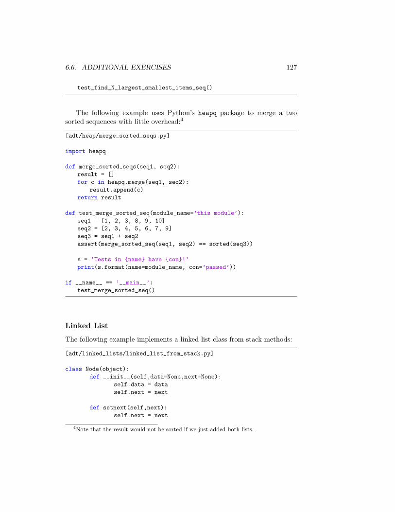
6.6. ADDITIONAL EXERCISES 127
test_find_N_largest_smallest_items_seq()
The following example uses Python’s heapq package to merge a twosorted sequences with little overhead:4
[adt/heap/merge_sorted_seqs.py]
import heapq
def merge_sorted_seqs(seq1, seq2):result = []for c in heapq.merge(seq1, seq2):
result.append(c)return result
def test_merge_sorted_seq(module_name=’this module’):seq1 = [1, 2, 3, 8, 9, 10]seq2 = [2, 3, 4, 5, 6, 7, 9]seq3 = seq1 + seq2assert(merge_sorted_seq(seq1, seq2) == sorted(seq3))
s = ’Tests in {name} have {con}!’print(s.format(name=module_name, con=’passed’))
if __name__ == ’__main__’:test_merge_sorted_seq()
Linked List
The following example implements a linked list class from stack methods:
[adt/linked_lists/linked_list_from_stack.py]
class Node(object):def __init__(self,data=None,next=None):
self.data = dataself.next = next
def setnext(self,next):self.next = next
4Note that the result would not be sorted if we just added both lists.
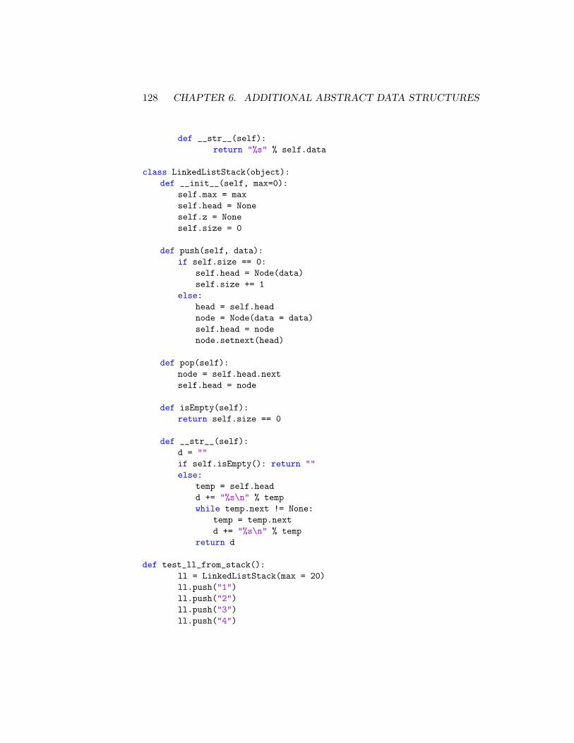
128 CHAPTER 6. ADDITIONAL ABSTRACT DATA STRUCTURES
def __str__(self):return "%s" % self.data
class LinkedListStack(object):def __init__(self, max=0):
self.max = maxself.head = Noneself.z = Noneself.size = 0
def push(self, data):if self.size == 0:
self.head = Node(data)self.size += 1
else:head = self.headnode = Node(data = data)self.head = nodenode.setnext(head)
def pop(self):node = self.head.nextself.head = node
def isEmpty(self):return self.size == 0
def __str__(self):d = ""if self.isEmpty(): return ""else:
temp = self.headd += "%s\n" % tempwhile temp.next != None:
temp = temp.nextd += "%s\n" % temp
return d
def test_ll_from_stack():ll = LinkedListStack(max = 20)ll.push("1")ll.push("2")ll.push("3")ll.push("4")
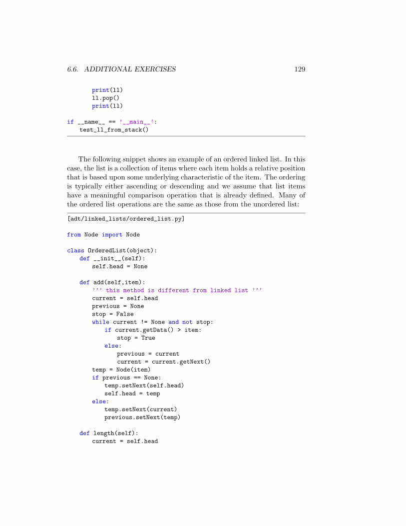
6.6. ADDITIONAL EXERCISES 129
print(ll)ll.pop()print(ll)
if __name__ == ’__main__’:test_ll_from_stack()
The following snippet shows an example of an ordered linked list. In thiscase, the list is a collection of items where each item holds a relative positionthat is based upon some underlying characteristic of the item. The orderingis typically either ascending or descending and we assume that list itemshave a meaningful comparison operation that is already defined. Many ofthe ordered list operations are the same as those from the unordered list:
[adt/linked_lists/ordered_list.py]
from Node import Node
class OrderedList(object):def __init__(self):
self.head = None
def add(self,item):’’’ this method is different from linked list ’’’current = self.headprevious = Nonestop = Falsewhile current != None and not stop:
if current.getData() > item:stop = True
else:previous = currentcurrent = current.getNext()
temp = Node(item)if previous == None:
temp.setNext(self.head)self.head = temp
else:temp.setNext(current)previous.setNext(temp)
def length(self):current = self.head
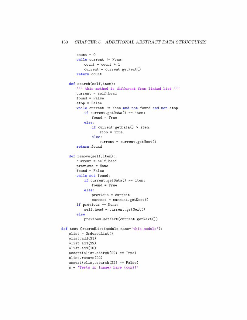
130 CHAPTER 6. ADDITIONAL ABSTRACT DATA STRUCTURES
count = 0while current != None:
count = count + 1current = current.getNext()
return count
def search(self,item):’’’ this method is different from linked list ’’’current = self.headfound = Falsestop = Falsewhile current != None and not found and not stop:
if current.getData() == item:found = True
else:if current.getData() > item:
stop = Trueelse:
current = current.getNext()return found
def remove(self,item):current = self.headprevious = Nonefound = Falsewhile not found:
if current.getData() == item:found = True
else:previous = currentcurrent = current.getNext()
if previous == None:self.head = current.getNext()
else:previous.setNext(current.getNext())
def test_OrderedList(module_name=’this module’):olist = OrderedList()olist.add(31)olist.add(22)olist.add(10)assert(olist.search(22) == True)olist.remove(22)assert(olist.search(22) == False)s = ’Tests in {name} have {con}!’
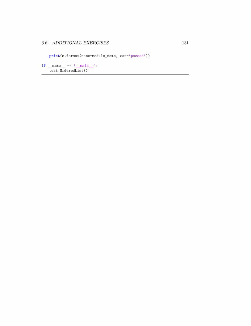
6.6. ADDITIONAL EXERCISES 131
print(s.format(name=module_name, con=’passed’))
if __name__ == ’__main__’:test_OrderedList()

132 CHAPTER 6. ADDITIONAL ABSTRACT DATA STRUCTURES
Chapter 7
Asymptotic Analysis
Asymptotic analysis is a method to describe the limiting behavior and theperformance of algorithms when applied to very large input datasets. Tounderstand why asymptotic analysis is important, suppose you have to sorta billion of numbers (n = 109)1 in a common desktop computer. Supposethat this computer has a CPU clock time of 1 GHz, which roughly meansthat it executes 109 processor cycles (or operations) per second.2 Then, foran algorithm that has a runtime of O(n2), it would take approximately onebillion of seconds to finish the sorting (in the worst case) which means oneentire year!
Another way of visualizing the importance of asymptotic analysis is di-rectly looking to the function’s behaviour. In the Fig. 7 we have manyclasses of functions plotted together and it is clear that when n increases,the number of operations for any polynomial or exponential algorithm isinfeasible.
7.1 Complexity Classes
A complexity class is a set of problems with related complexity. A reductionis a transformation of one problem into another problem which is at leastas difficult as the original problem. The most commonly used reduction
1Remember that for memory gigabytes means 10243 = 230 bytes and for storage itmeans 10003 = 109 bytes. Also, integers usually take 2 or 4 bytes each. However, for thisexample we are simplifying this by saying that a ‘number’ has 1 byte.
2In this exercise we are not considering other factors that would make the processingslower, such as RAM latency, copy cache operations, etc.
133
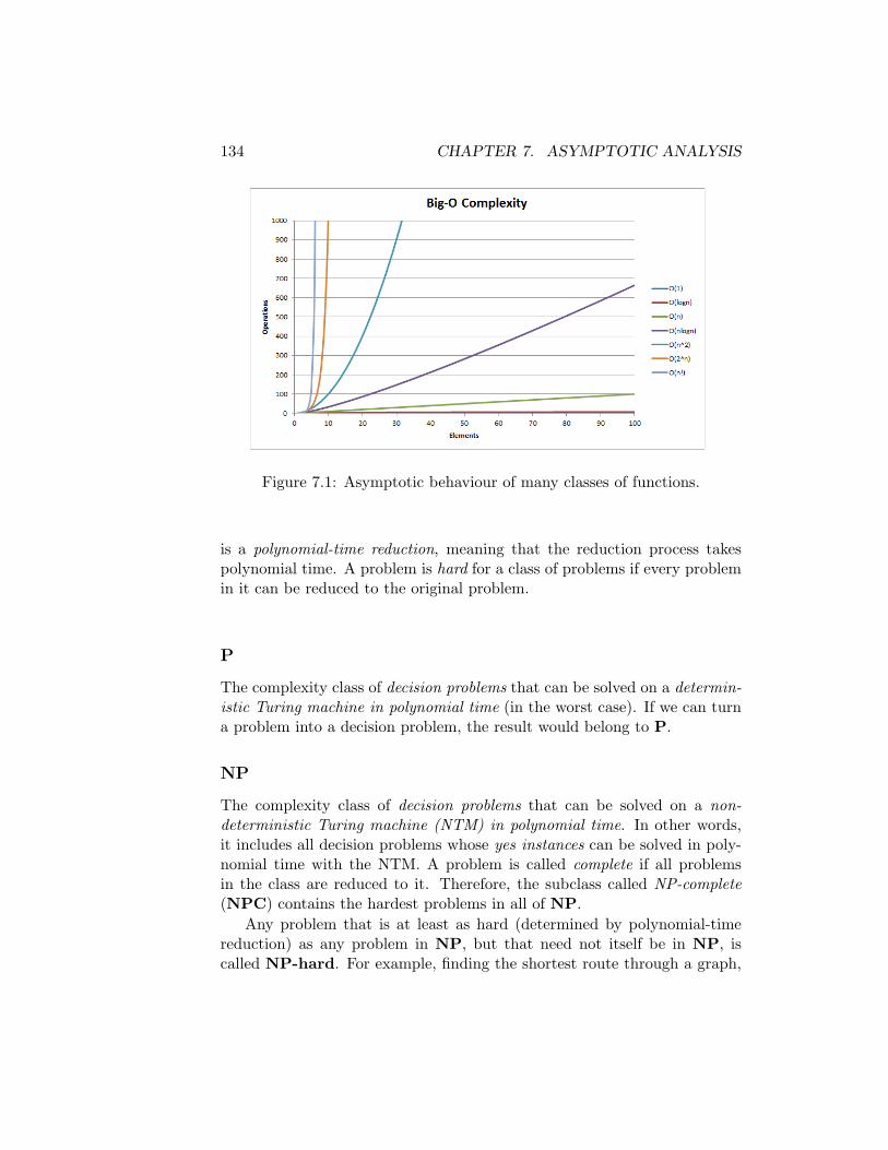
134 CHAPTER 7. ASYMPTOTIC ANALYSIS
Figure 7.1: Asymptotic behaviour of many classes of functions.
is a polynomial-time reduction, meaning that the reduction process takespolynomial time. A problem is hard for a class of problems if every problemin it can be reduced to the original problem.
P
The complexity class of decision problems that can be solved on a determin-istic Turing machine in polynomial time (in the worst case). If we can turna problem into a decision problem, the result would belong to P.
NP
The complexity class of decision problems that can be solved on a non-deterministic Turing machine (NTM) in polynomial time. In other words,it includes all decision problems whose yes instances can be solved in poly-nomial time with the NTM. A problem is called complete if all problemsin the class are reduced to it. Therefore, the subclass called NP-complete(NPC) contains the hardest problems in all of NP.
Any problem that is at least as hard (determined by polynomial-timereduction) as any problem in NP, but that need not itself be in NP, iscalled NP-hard. For example, finding the shortest route through a graph,
7.2. RECURSION 135
which is called the Travelling Salesman (or Salesrep) problem (TSP).
P=NP?
The class co-NP is the class of the complements of NP problems. For every“yes” answer, we have the “no”, and vice versa. If NP is truly asymmetric,then these two classes are different. Although there is overlap between thembecause all of P lies in their intersection: both the yes and no instances inP can be solved in polynomial time with an NTM.
What would happen if a NPC was found in a intersection of N andco-NP? First, it would mean that all of NP would be inside co-NP, so wewould show NP = co-NP and the asymmetry would disappear. Second,since all of P is in this intersection, P = NP. If P = NP, we could solveany (decision) problem that had a practical (verifiable) solution.
However, it is (strongly) believed that NP and co-NP are different. Forinstance, no polynomial solution to the problem of factoring numbers wasfound, and this problem is in both NP and co-NP.
7.2 Recursion
The three laws of recursion are:
1. A recursive algorithm must have a base case.
2. A recursive algorithm must change its state and move toward the basecase.
3. A recursive algorithm must call itself, recursively.
For every recursive call, the recursive function has to allocate memoryon the stack for arguments, return address, and local variables, costing timeto push and pop these data onto the stack. Recursive algorithms take atleast O(n) space where n is the depth of the recursive call.
Recursion is very costly when there are duplicated calculations and/orthere are overlap among subproblems. In some cases this can cause the stackto overflow. For this reason, where subproblems overlap, iterative solutionsmight be a better approach. For example, in the case of the Fibonacciseries, the iterative solution runs on O(n) while the recursive solution runson exponential runtime.
136 CHAPTER 7. ASYMPTOTIC ANALYSIS
Recursive Relations
To describe the running time of recursive functions, we use recursive rela-tions:
T (n) = a · T (g(n)) + f(n),
where a represents the number of recursive calls, g(n) is the size of eachsubproblem to be solved recursively, and f(n) is any extra work done in thefunction. The following table shows examples of recursive relations:
T (n) = T (n− 1) + 1 O(n) Processing a sequence
T (n) = T (n− 1) + n O(n2) Handshake problem
T (n) = 2T (n− 1) + 1 O(2n) Towers of Hanoi
T (n) = T (n/2) + 1 O(ln n) Binary search
T (n) = T (n/2) + n O(n) Randomized select
T (n) = 2T (n/2) + 1 O(n) Tree transversal
T (n) = 2T (n/2) + n O(n ln n) Sort by divide and conquer
Divide and Conquer Algorithms
Recurrences for the divide and conquer algorithms have the form:
T (n) = a · T (n/b) + f(n),
where we have a recursive calls, each with a percentage 1/b of the dataset.Summing to this, the algorithm does f(n) of work. To reach the problem ofT(1) = 1 in the final instance (leaf, as we will learn when we study trees),the height is defined as h = lnb n, Fig. 7.2.
7.3 Runtime in Functions
We are now ready to estimate algorithm runtimes. First of all, if the al-gorithm does not have any recursive calling, we only need to analyse itsdata structures and flow blocks. In this case, complexities of code blocksexecuted one after the other are just added and complexities of nested loopsare multiplied.
If the algorithm has recursive calls, we can use the recursive functionsfrom the previous section to find the runtime. When we write a recurrencerelation for a function, we must write two equations, one for the general caseand one for the base case (that should be O(1), so that T (1) = 1). Keepingthis in mind, let us take a look at the example of the algorithm to find thenth element in a Fibonacci sequence, which is known as to be exponential:
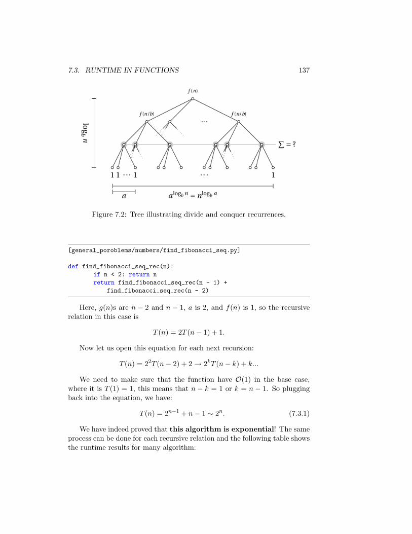
7.3. RUNTIME IN FUNCTIONS 137
Figure 7.2: Tree illustrating divide and conquer recurrences.
[general_poroblems/numbers/find_fibonacci_seq.py]
def find_fibonacci_seq_rec(n):if n < 2: return nreturn find_fibonacci_seq_rec(n - 1) +
find_fibonacci_seq_rec(n - 2)
Here, g(n)s are n − 2 and n − 1, a is 2, and f(n) is 1, so the recursiverelation in this case is
T (n) = 2T (n− 1) + 1.
Now let us open this equation for each next recursion:
T (n) = 22T (n− 2) + 2→ 2kT (n− k) + k...
We need to make sure that the function have O(1) in the base case,where it is T (1) = 1, this means that n − k = 1 or k = n − 1. So pluggingback into the equation, we have:
T (n) = 2n−1 + n− 1 ∼ 2n. (7.3.1)
We have indeed proved that this algorithm is exponential! The sameprocess can be done for each recursive relation and the following table showsthe runtime results for many algorithm:
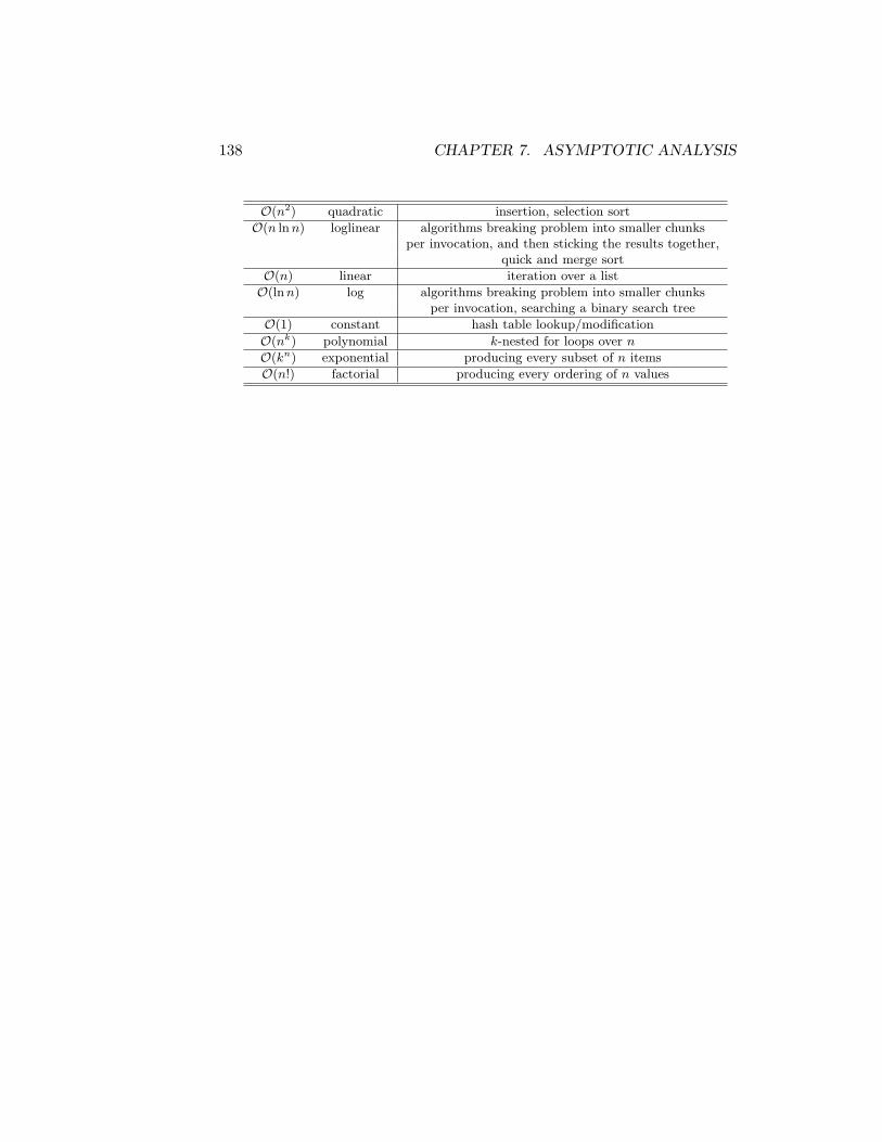
138 CHAPTER 7. ASYMPTOTIC ANALYSIS
O(n2) quadratic insertion, selection sort
O(n ln n) loglinear algorithms breaking problem into smaller chunksper invocation, and then sticking the results together,
quick and merge sort
O(n) linear iteration over a list
O(ln n) log algorithms breaking problem into smaller chunksper invocation, searching a binary search tree
O(1) constant hash table lookup/modification
O(nk) polynomial k-nested for loops over n
O(kn) exponential producing every subset of n items
O(n!) factorial producing every ordering of n values
Chapter 8
Sorting
The simplest way of sorting a group of items is to start by removing thesmallest item from the group, and putting it first. Then removing the nextsmallest, and putting it next and so on. This is clearly an O(n2) algo-rithm, so we need to find a better solution. In this chapter we will look atmany examples of sorting algorithms and analyse their characteristics andruntimes.
An in-place sort does not use any additional memory to do the sorting(for example, swapping elements in an array). A stable sort preserves therelative order of otherwise identical data elements (for example, if two dataelements have identical values, the one that was ahead of the other staysahead). In any comparison sort problem, a key is the value (or values) thatdetermines the sorting order. A comparison sort requires only that there is away to determine if a key is less than, equal to, or greater than another key.Most sorting algorithms are comparison sorts where the worst-case runningtime for such sorts can be no better than O(n ln n).
8.1 Quadratic Sort
Insertion Sort
Insertion sort is a simple sorting algorithm with best runtime case runtimeofO(n) and average and worst runtime cases ofO(n2). It sorts by repeatedlyinserting the next unsorted element in an initial sorted segment of the array.For small data sets, it can be preferable to more advanced algorithms suchas merge sort or quicksort if the list is already sorted (it is a good way toadd new elements to a presorted list):
139
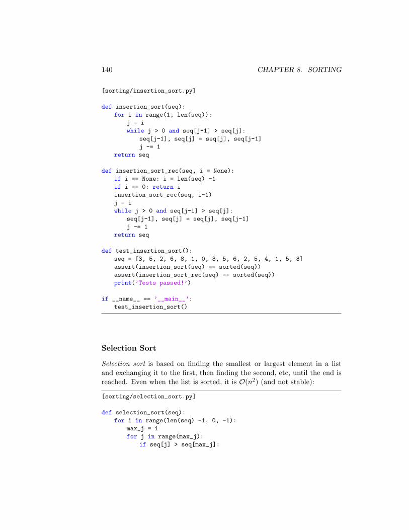
140 CHAPTER 8. SORTING
[sorting/insertion_sort.py]
def insertion_sort(seq):for i in range(1, len(seq)):
j = iwhile j > 0 and seq[j-1] > seq[j]:
seq[j-1], seq[j] = seq[j], seq[j-1]j -= 1
return seq
def insertion_sort_rec(seq, i = None):if i == None: i = len(seq) -1if i == 0: return iinsertion_sort_rec(seq, i-1)j = iwhile j > 0 and seq[j-i] > seq[j]:
seq[j-1], seq[j] = seq[j], seq[j-1]j -= 1
return seq
def test_insertion_sort():seq = [3, 5, 2, 6, 8, 1, 0, 3, 5, 6, 2, 5, 4, 1, 5, 3]assert(insertion_sort(seq) == sorted(seq))assert(insertion_sort_rec(seq) == sorted(seq))print(’Tests passed!’)
if __name__ == ’__main__’:test_insertion_sort()
Selection Sort
Selection sort is based on finding the smallest or largest element in a listand exchanging it to the first, then finding the second, etc, until the end isreached. Even when the list is sorted, it is O(n2) (and not stable):
[sorting/selection_sort.py]
def selection_sort(seq):for i in range(len(seq) -1, 0, -1):
max_j = ifor j in range(max_j):
if seq[j] > seq[max_j]:
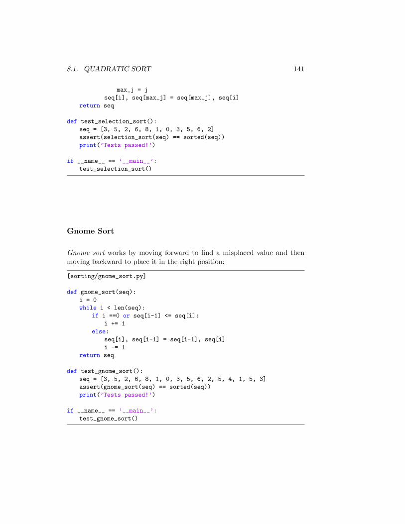
8.1. QUADRATIC SORT 141
max_j = jseq[i], seq[max_j] = seq[max_j], seq[i]
return seq
def test_selection_sort():seq = [3, 5, 2, 6, 8, 1, 0, 3, 5, 6, 2]assert(selection_sort(seq) == sorted(seq))print(’Tests passed!’)
if __name__ == ’__main__’:test_selection_sort()
Gnome Sort
Gnome sort works by moving forward to find a misplaced value and thenmoving backward to place it in the right position:
[sorting/gnome_sort.py]
def gnome_sort(seq):i = 0while i < len(seq):
if i ==0 or seq[i-1] <= seq[i]:i += 1
else:seq[i], seq[i-1] = seq[i-1], seq[i]i -= 1
return seq
def test_gnome_sort():seq = [3, 5, 2, 6, 8, 1, 0, 3, 5, 6, 2, 5, 4, 1, 5, 3]assert(gnome_sort(seq) == sorted(seq))print(’Tests passed!’)
if __name__ == ’__main__’:test_gnome_sort()
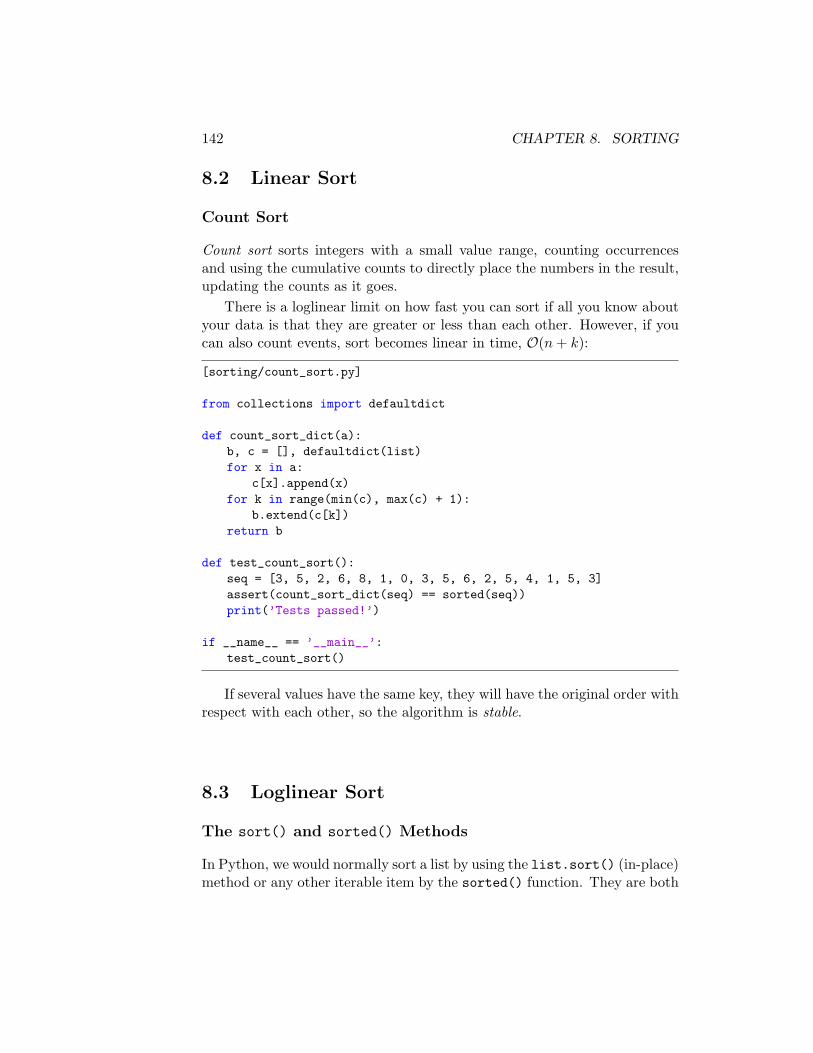
142 CHAPTER 8. SORTING
8.2 Linear Sort
Count Sort
Count sort sorts integers with a small value range, counting occurrencesand using the cumulative counts to directly place the numbers in the result,updating the counts as it goes.
There is a loglinear limit on how fast you can sort if all you know aboutyour data is that they are greater or less than each other. However, if youcan also count events, sort becomes linear in time, O(n + k):
[sorting/count_sort.py]
from collections import defaultdict
def count_sort_dict(a):b, c = [], defaultdict(list)for x in a:
c[x].append(x)for k in range(min(c), max(c) + 1):
b.extend(c[k])return b
def test_count_sort():seq = [3, 5, 2, 6, 8, 1, 0, 3, 5, 6, 2, 5, 4, 1, 5, 3]assert(count_sort_dict(seq) == sorted(seq))print(’Tests passed!’)
if __name__ == ’__main__’:test_count_sort()
If several values have the same key, they will have the original order withrespect with each other, so the algorithm is stable.
8.3 Loglinear Sort
The sort() and sorted() Methods
In Python, we would normally sort a list by using the list.sort() (in-place)method or any other iterable item by the sorted() function. They are both
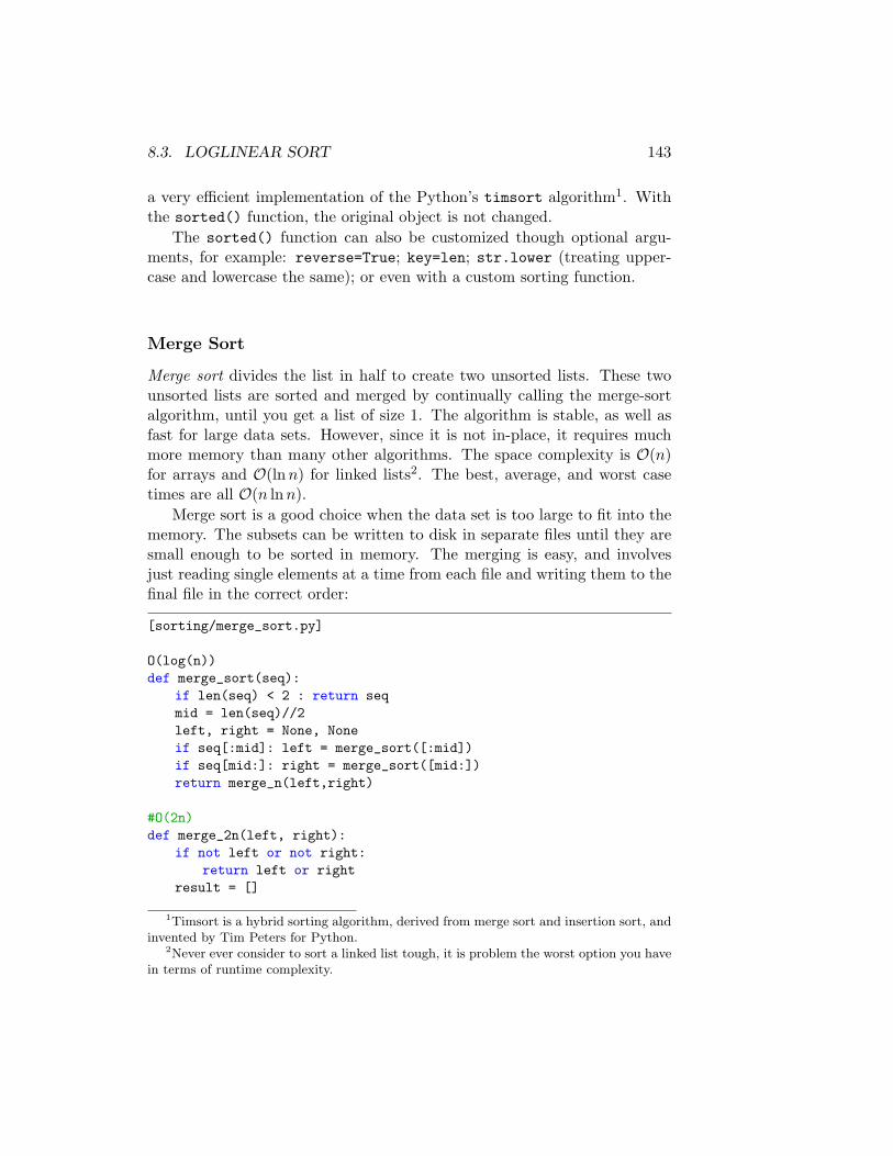
8.3. LOGLINEAR SORT 143
a very efficient implementation of the Python’s timsort algorithm1. Withthe sorted() function, the original object is not changed.
The sorted() function can also be customized though optional argu-ments, for example: reverse=True; key=len; str.lower (treating upper-case and lowercase the same); or even with a custom sorting function.
Merge Sort
Merge sort divides the list in half to create two unsorted lists. These twounsorted lists are sorted and merged by continually calling the merge-sortalgorithm, until you get a list of size 1. The algorithm is stable, as well asfast for large data sets. However, since it is not in-place, it requires muchmore memory than many other algorithms. The space complexity is O(n)for arrays and O(ln n) for linked lists2. The best, average, and worst casetimes are all O(n ln n).
Merge sort is a good choice when the data set is too large to fit into thememory. The subsets can be written to disk in separate files until they aresmall enough to be sorted in memory. The merging is easy, and involvesjust reading single elements at a time from each file and writing them to thefinal file in the correct order:
[sorting/merge_sort.py]
O(log(n))def merge_sort(seq):
if len(seq) < 2 : return seqmid = len(seq)//2left, right = None, Noneif seq[:mid]: left = merge_sort([:mid])if seq[mid:]: right = merge_sort([mid:])return merge_n(left,right)
#O(2n)def merge_2n(left, right):
if not left or not right:return left or right
result = []
1Timsort is a hybrid sorting algorithm, derived from merge sort and insertion sort, andinvented by Tim Peters for Python.
2Never ever consider to sort a linked list tough, it is problem the worst option you havein terms of runtime complexity.
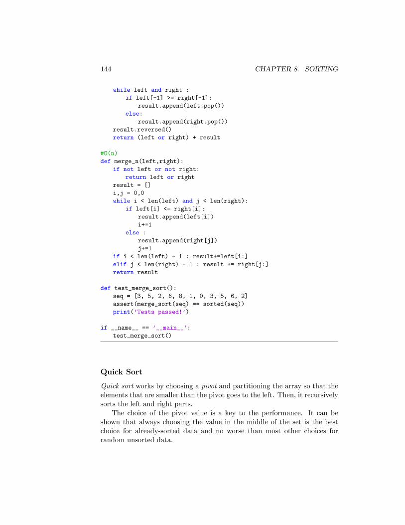
144 CHAPTER 8. SORTING
while left and right :if left[-1] >= right[-1]:
result.append(left.pop())else:
result.append(right.pop())result.reversed()return (left or right) + result
#O(n)def merge_n(left,right):
if not left or not right:return left or right
result = []i,j = 0,0while i < len(left) and j < len(right):
if left[i] <= right[i]:result.append(left[i])i+=1
else :result.append(right[j])j+=1
if i < len(left) - 1 : result+=left[i:]elif j < len(right) - 1 : result += right[j:]return result
def test_merge_sort():seq = [3, 5, 2, 6, 8, 1, 0, 3, 5, 6, 2]assert(merge_sort(seq) == sorted(seq))print(’Tests passed!’)
if __name__ == ’__main__’:test_merge_sort()
Quick Sort
Quick sort works by choosing a pivot and partitioning the array so that theelements that are smaller than the pivot goes to the left. Then, it recursivelysorts the left and right parts.
The choice of the pivot value is a key to the performance. It can beshown that always choosing the value in the middle of the set is the bestchoice for already-sorted data and no worse than most other choices forrandom unsorted data.
8.3. LOGLINEAR SORT 145
The worst case is O(n2) in the rare cases when partitioning keeps pro-ducing a region of n − 1 elements (when the pivot is the minimum value).The best case produces two n/2-sized lists. This and the average case areboth O(n ln n). The algorithm is not stable.
[sorting/quick_sort.py]
def quick_sort(seq):if len(seq) < 2 : return seqmid = len(seq)//2pi = seq[mid]seq = seq[:mid] + seq[mid+1:]lo = [x for x in seq if x <= pi]hi = [x for x in seq if x > pi]return quick_sort(lo) + [pi] + quick_sort(hi)
def test_quick_sort():seq = [3, 5, 2, 6, 8, 1, 0, 3, 5, 6, 2]assert(quick_sort(seq) == sorted(seq))assert(quick_sort_divided(seq) == sorted(seq))print(’Tests passed!’)
if __name__ == ’__main__’:test_quick_sort()
Heap Sort
Heap sort is similar to a selection sort, except that the unsorted region is aheap, so finding the largest element n times gives a loglinear runtime.
In a heap, for every node other than the root, the value of the node is atleast (at most) the value of its parent. Thus, the smallest (largest) element isstored at the root and the subtrees rooted at a node contain larger (smaller)values than does the node itself.
Although the insertion is only O(1), the performance of validating (theheap order) is O(ln n). Searching (traversing) is O(n). In Python, a heapsort can be implemented by pushing all values onto a heap and then poppingoff the smallest values one at a time:
[sorting/heap_sort1.py]
import heapq
146 CHAPTER 8. SORTING
def heap_sort1(seq):’’’ heap sort with Pythons heapq ’’’h = []for value in seq:
heapq.heappush(h, value)return [heapq.heappop(h) for i in range(len(h))]
def test_heap_sort1():seq = [3, 5, 2, 6, 8, 1, 0, 3, 5, 6, 2]assert(heap_sort1(seq) == sorted(seq))print(’Tests passed!’)
if __name__ == ’__main__’:test_heap_sort1()
If we decide to use the heap class that we have from the last chapters,we can write a heap sort simply by:
[sorting/heap_sort2.py]
from heap import Heap
def heap_sort2(seq):heap = Heap(seq)res = []for i in range(len(seq)):
res.insert(0, heap.extract_max())return res
def test_heap_sort2():seq = [3, 5, 2, 6, 8, 1, 0, 3, 5, 6, 2]assert(heap_sort2(seq) == sorted(seq))print(’Tests passed!’)
if __name__ == ’__main__’:test_heap_sort2()
Finally, we can also write our heap sort explicitly:
[sorting/heap_sort3.py]
8.3. LOGLINEAR SORT 147
def heap_sort3(seq):for start in range((len(seq)-2)//2, -1, -1):
siftdown(seq, start, len(seq)-1)for end in range(len(seq)-1, 0, -1):
seq[end], seq[0] = seq[0], seq[end]siftdown(seq, 0, end - 1)
return seq
def siftdown(seq, start, end):root = startwhile True:
child = root * 2 + 1if child > end: breakif child + 1 <= end and seq[child] < seq[child + 1]:
child += 1if seq[root] < seq[child]:
seq[root], seq[child] = seq[child], seq[root]root = child
else:break
def test_heap_sort():seq = [3, 5, 2, 6, 8, 1, 0, 3, 5, 6, 2]assert(heap_sort3(seq) == sorted(seq))print(’Tests passed!’)
if __name__ == ’__main__’:test_heap_sort3()
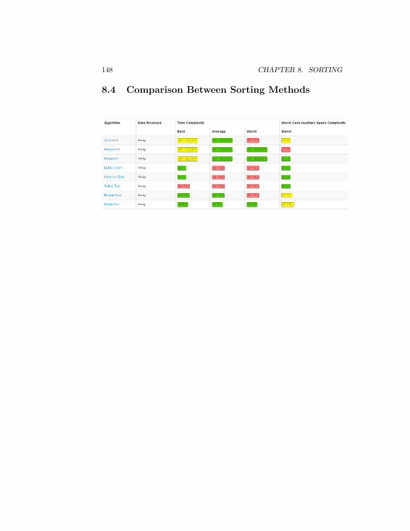
148 CHAPTER 8. SORTING
8.4 Comparison Between Sorting Methods
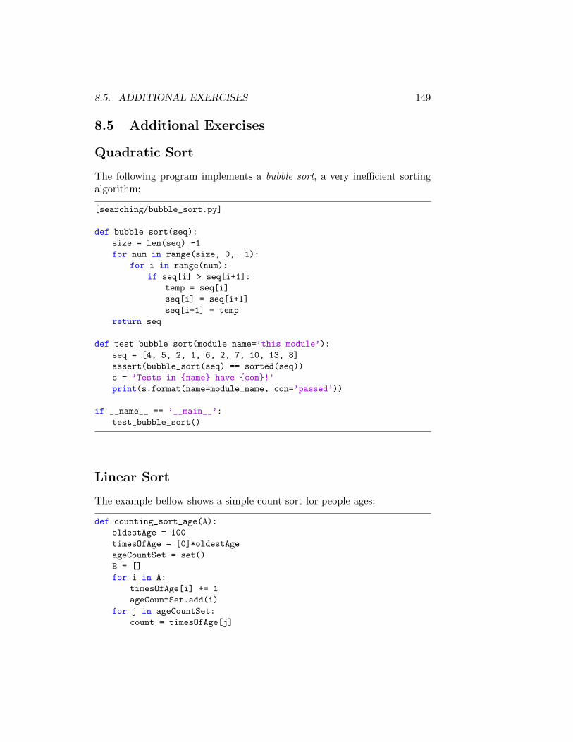
8.5. ADDITIONAL EXERCISES 149
8.5 Additional Exercises
Quadratic Sort
The following program implements a bubble sort, a very inefficient sortingalgorithm:
[searching/bubble_sort.py]
def bubble_sort(seq):size = len(seq) -1for num in range(size, 0, -1):
for i in range(num):if seq[i] > seq[i+1]:
temp = seq[i]seq[i] = seq[i+1]seq[i+1] = temp
return seq
def test_bubble_sort(module_name=’this module’):seq = [4, 5, 2, 1, 6, 2, 7, 10, 13, 8]assert(bubble_sort(seq) == sorted(seq))s = ’Tests in {name} have {con}!’print(s.format(name=module_name, con=’passed’))
if __name__ == ’__main__’:test_bubble_sort()
Linear Sort
The example bellow shows a simple count sort for people ages:
def counting_sort_age(A):oldestAge = 100timesOfAge = [0]*oldestAgeageCountSet = set()B = []for i in A:
timesOfAge[i] += 1ageCountSet.add(i)
for j in ageCountSet:count = timesOfAge[j]
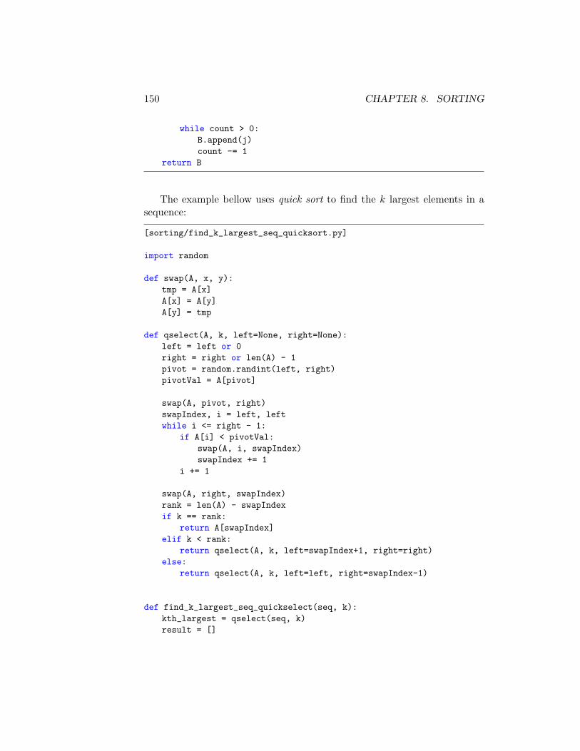
150 CHAPTER 8. SORTING
while count > 0:B.append(j)count -= 1
return B
The example bellow uses quick sort to find the k largest elements in asequence:
[sorting/find_k_largest_seq_quicksort.py]
import random
def swap(A, x, y):tmp = A[x]A[x] = A[y]A[y] = tmp
def qselect(A, k, left=None, right=None):left = left or 0right = right or len(A) - 1pivot = random.randint(left, right)pivotVal = A[pivot]
swap(A, pivot, right)swapIndex, i = left, leftwhile i <= right - 1:
if A[i] < pivotVal:swap(A, i, swapIndex)swapIndex += 1
i += 1
swap(A, right, swapIndex)rank = len(A) - swapIndexif k == rank:
return A[swapIndex]elif k < rank:
return qselect(A, k, left=swapIndex+1, right=right)else:
return qselect(A, k, left=left, right=swapIndex-1)
def find_k_largest_seq_quickselect(seq, k):kth_largest = qselect(seq, k)result = []
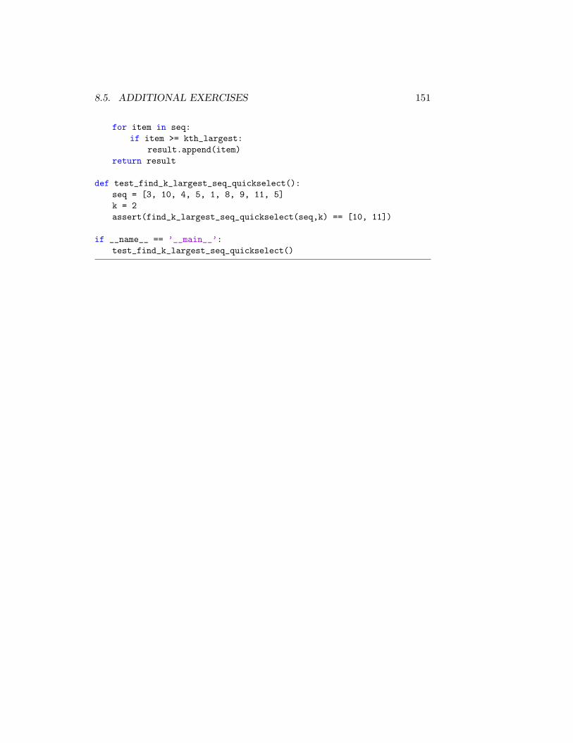
8.5. ADDITIONAL EXERCISES 151
for item in seq:if item >= kth_largest:
result.append(item)return result
def test_find_k_largest_seq_quickselect():seq = [3, 10, 4, 5, 1, 8, 9, 11, 5]k = 2assert(find_k_largest_seq_quickselect(seq,k) == [10, 11])
if __name__ == ’__main__’:test_find_k_largest_seq_quickselect()

152 CHAPTER 8. SORTING
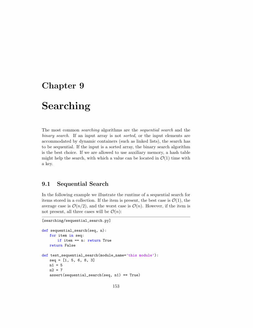
Chapter 9
Searching
The most common searching algorithms are the sequential search and thebinary search. If an input array is not sorted, or the input elements areaccommodated by dynamic containers (such as linked lists), the search hasto be sequential. If the input is a sorted array, the binary search algorithmis the best choice. If we are allowed to use auxiliary memory, a hash tablemight help the search, with which a value can be located in O(1) time witha key.
9.1 Sequential Search
In the following example we illustrate the runtime of a sequential search foritems stored in a collection. If the item is present, the best case is O(1), theaverage case is O(n/2), and the worst case is O(n). However, if the item isnot present, all three cases will be O(n):
[searching/sequential_search.py]
def sequential_search(seq, n):for item in seq:
if item == n: return Truereturn False
def test_sequential_search(module_name=’this module’):seq = [1, 5, 6, 8, 3]n1 = 5n2 = 7assert(sequential_search(seq, n1) == True)
153
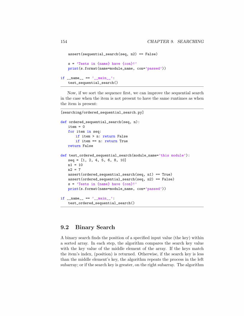
154 CHAPTER 9. SEARCHING
assert(sequential_search(seq, n2) == False)
s = ’Tests in {name} have {con}!’print(s.format(name=module_name, con=’passed’))
if __name__ == ’__main__’:test_sequential_search()
Now, if we sort the sequence first, we can improve the sequential searchin the case when the item is not present to have the same runtimes as whenthe item is present:
[searching/ordered_sequential_search.py]
def ordered_sequential_search(seq, n):item = 0for item in seq:
if item > n: return Falseif item == n: return True
return False
def test_ordered_sequential_search(module_name=’this module’):seq = [1, 2, 4, 5, 6, 8, 10]n1 = 10n2 = 7assert(ordered_sequential_search(seq, n1) == True)assert(ordered_sequential_search(seq, n2) == False)s = ’Tests in {name} have {con}!’print(s.format(name=module_name, con=’passed’))
if __name__ == ’__main__’:test_ordered_sequential_search()
9.2 Binary Search
A binary search finds the position of a specified input value (the key) withina sorted array. In each step, the algorithm compares the search key valuewith the key value of the middle element of the array. If the keys matchthe item’s index, (position) is returned. Otherwise, if the search key is lessthan the middle element’s key, the algorithm repeats the process in the leftsubarray; or if the search key is greater, on the right subarray. The algorithm
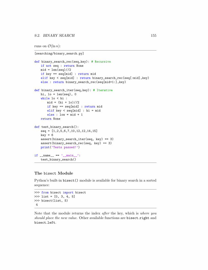
9.2. BINARY SEARCH 155
runs on O(ln n):
[searching/binary_search.py]
def binary_search_rec(seq,key): # Recursiveif not seq : return Nonemid = len(seq)//2if key == seq[mid] : return midelif key < seq[mid] : return binary_search_rec(seq[:mid],key)else : return binary_search_rec(seq[mid+1:],key)
def binary_search_iter(seq,key): # Iterativehi, lo = len(seq), 0while lo < hi :
mid = (hi + lo)//2if key == seq[mid] : return midelif key < seq[mid] : hi = midelse : low = mid + 1
return None
def test_binary_search():seq = [1,2,5,6,7,10,12,12,14,15]key = 6assert(binary_search_iter(seq, key) == 3)assert(binary_search_rec(seq, key) == 3)print(’Tests passed!’)
if __name__ == ’__main__’:test_binary_search()
The bisect Module
Python’s built-in bisect() module is available for binary search in a sortedsequence:
>>> from bisect import bisect>>> list = [0, 3, 4, 5]>>> bisect(list, 5)4
Note that the module returns the index after the key, which is where youshould place the new value. Other available functions are bisect right andbisect left.
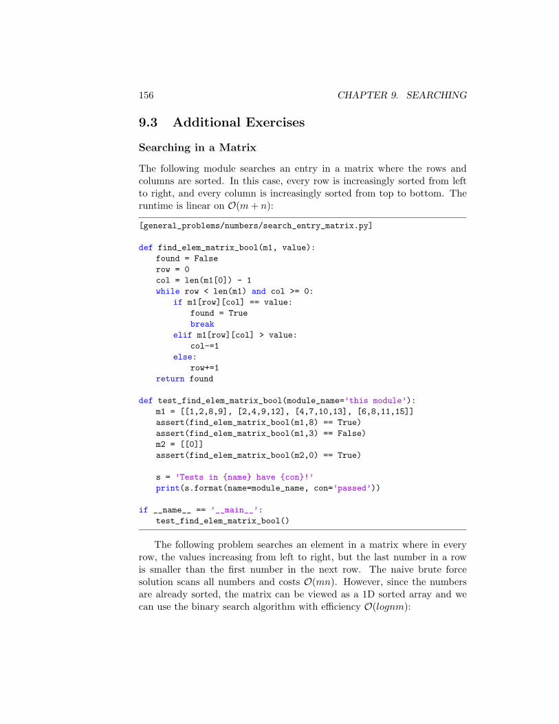
156 CHAPTER 9. SEARCHING
9.3 Additional Exercises
Searching in a Matrix
The following module searches an entry in a matrix where the rows andcolumns are sorted. In this case, every row is increasingly sorted from leftto right, and every column is increasingly sorted from top to bottom. Theruntime is linear on O(m + n):
[general_problems/numbers/search_entry_matrix.py]
def find_elem_matrix_bool(m1, value):found = Falserow = 0col = len(m1[0]) - 1while row < len(m1) and col >= 0:
if m1[row][col] == value:found = Truebreak
elif m1[row][col] > value:col-=1
else:row+=1
return found
def test_find_elem_matrix_bool(module_name=’this module’):m1 = [[1,2,8,9], [2,4,9,12], [4,7,10,13], [6,8,11,15]]assert(find_elem_matrix_bool(m1,8) == True)assert(find_elem_matrix_bool(m1,3) == False)m2 = [[0]]assert(find_elem_matrix_bool(m2,0) == True)
s = ’Tests in {name} have {con}!’print(s.format(name=module_name, con=’passed’))
if __name__ == ’__main__’:test_find_elem_matrix_bool()
The following problem searches an element in a matrix where in everyrow, the values increasing from left to right, but the last number in a rowis smaller than the first number in the next row. The naive brute forcesolution scans all numbers and costs O(mn). However, since the numbersare already sorted, the matrix can be viewed as a 1D sorted array and wecan use the binary search algorithm with efficiency O(lognm):
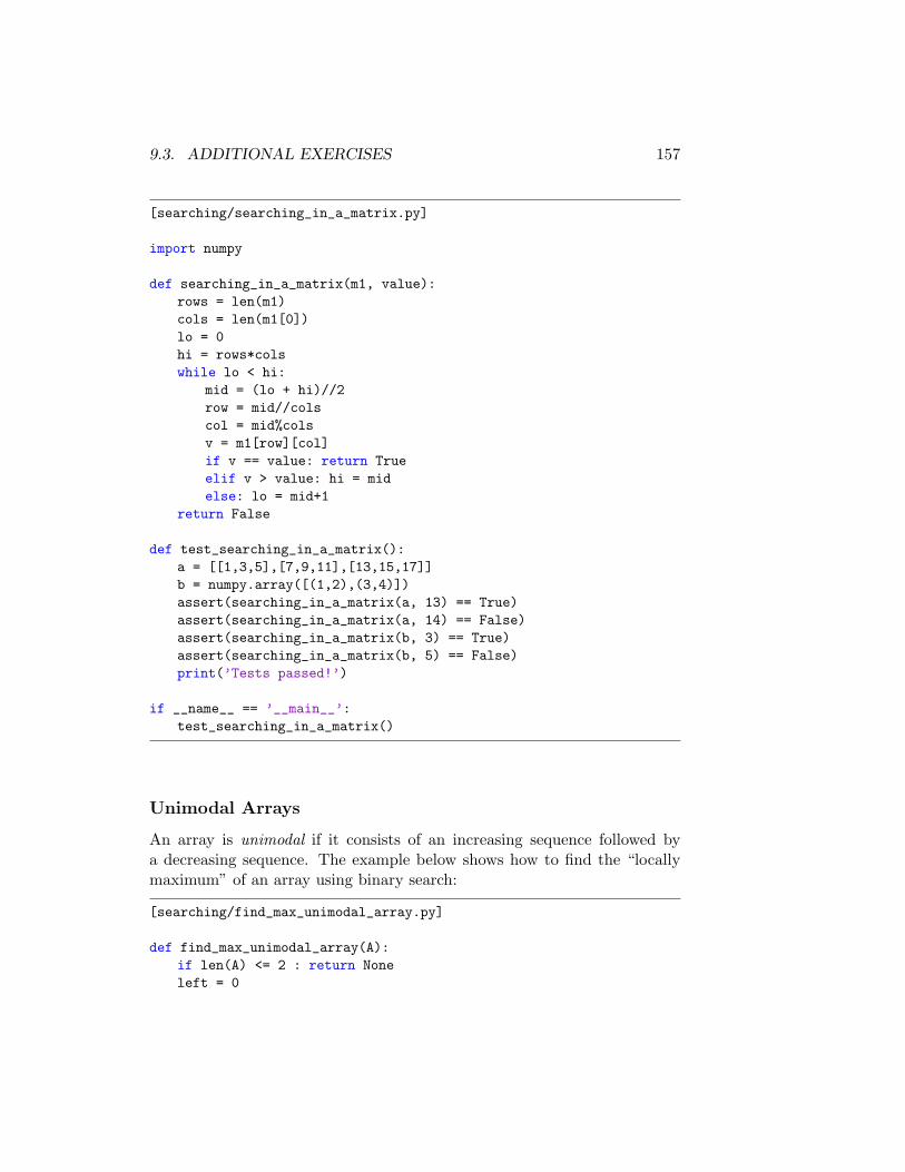
9.3. ADDITIONAL EXERCISES 157
[searching/searching_in_a_matrix.py]
import numpy
def searching_in_a_matrix(m1, value):rows = len(m1)cols = len(m1[0])lo = 0hi = rows*colswhile lo < hi:
mid = (lo + hi)//2row = mid//colscol = mid%colsv = m1[row][col]if v == value: return Trueelif v > value: hi = midelse: lo = mid+1
return False
def test_searching_in_a_matrix():a = [[1,3,5],[7,9,11],[13,15,17]]b = numpy.array([(1,2),(3,4)])assert(searching_in_a_matrix(a, 13) == True)assert(searching_in_a_matrix(a, 14) == False)assert(searching_in_a_matrix(b, 3) == True)assert(searching_in_a_matrix(b, 5) == False)print(’Tests passed!’)
if __name__ == ’__main__’:test_searching_in_a_matrix()
Unimodal Arrays
An array is unimodal if it consists of an increasing sequence followed bya decreasing sequence. The example below shows how to find the “locallymaximum” of an array using binary search:
[searching/find_max_unimodal_array.py]
def find_max_unimodal_array(A):if len(A) <= 2 : return Noneleft = 0
158 CHAPTER 9. SEARCHING
right = len(A)-1while right > left +1:
mid = (left + right)//2if A[mid] > A[mid-1] and A[mid] > A[mid+1]:
return A[mid]elif A[mid] > A[mid-1] and A[mid] < A[mid+1]:
left = midelse:
right = midreturn None
def test_find_max_unimodal_array():seq = [1, 2, 5, 6, 7, 10, 12, 9, 8, 7, 6]assert(find_max_unimodal_array(seq) == 12)print(’Tests passed!’)
if __name__ == ’__main__’:test_find_max_unimodal_array()
Calculating Square Roots
The example bellow implements the square root of a number using binarysearch:
[searching/find_sqrt_bin_search.py]
def find_sqrt_bin_search(n, error=0.001):lower = n < 1 and n or 1upper = n < 1 and 1 or nmid = lower + (upper - lower) / 2.0square = mid * midwhile abs(square - n) > error:
if square < n:lower = mid
else:upper = mid
mid = lower + (upper - lower) / 2.0square = mid * mid
return mid
def test_ind_sqrt_bin_search():number = 9assert(find_sqrt_bin_search(number) == 3)
9.3. ADDITIONAL EXERCISES 159
print(’Tests passed!’)
if __name__ == ’__main__’:test_ind_sqrt_bin_search()
Counting Frequency of Elements
The following example finds how many times a k element appears in a sortedlist. Since the array is sorted, binary search gives a O(logn) runtime:
[searching/find_time_occurence_list.py]
from binary_search import binary_search
def find_time_occurrence_list(seq, k):index_some_k = binary_serch(seq, k)count = 1sizet = len(seq)for i in range(index_some_k+1, sizet): # go up
if seq[i] == k: count +=1else: break
for i in range(index_some_k-1, -1, -1): # go downif seq[i] == k: count +=1else: break
return count
def test_find_time_occurrence_list():seq = [1,2,2,2,2,2,2,5,6,6,7,8,9]k = 2assert(find_time_occurrence_list(seq, k) == 6)print(’Tests passed!’)
if __name__ == ’__main__’:test_find_time_occurrence_list()
Intersection of Arrays
The snippet bellow shows three ways to perform the intersection of twosorted arrays. The simplest way is to use sets, however this will not preservethe ordering. The second example uses an adaptation of the merge sort. The
160 CHAPTER 9. SEARCHING
third example is suitable when one of the arrays is much larger than other.In this case, binary search is the best option:
[searching/intersection_two_arrays.py]
def intersection_two_arrays_sets(seq1, seq2):’’’ find the intersection of two arrays using set proprieties
’’’set1 = set(seq1)set2 = set(seq2)return set1.intersection(set2) #same as list(set1 & set2
def intersection_two_arrays_ms(seq1, seq2):’’’ find the intersection of two arrays using merge sort ’’’res = []while seq1 and seq2:
if seq1[-1] == seq2[-1]:res.append(seq1.pop())seq2.pop()
elif seq1[-1] > seq2[-1]:seq1.pop()
else:seq2.pop()
res.reverse()return res
from binary_search import binary_searchdef intersection_two_arrays_bs(seq1, seq2):
’’’ using binary search ’’’if len(seq1) > len(seq2): seq, key = seq1, seq2else: seq, key = seq2, seq1intersec = []for item in key:
if binary_search(seq, item):intersec.append(item)
return intersec
def test_intersection_two_arrays(module_name=’this module’):seq1 = [1,2,3,5,7,8]seq2 = [3,5,6]assert(set(intersection_two_arrays_sets(seq1,seq2)) ==
set([3,5]))
9.3. ADDITIONAL EXERCISES 161
assert(intersection_two_arrays_bs(seq1,seq2) == [3,5])assert(intersection_two_arrays_ms(seq1,seq2) == [3,5])s = ’Tests in {name} have {con}!’print(s.format(name=module_name, con=’passed’))
if __name__ == ’__main__’:test_intersection_two_arrays()

162 CHAPTER 9. SEARCHING
Chapter 10
Dynamic Programming
Dynamic programming is used to simplify a complicated problem by breakingit down into simpler subproblems by means of recursion. If a problem hasan optimal substructure and overlapping subproblems, it may be solved bydynamic programming.
Optimal substructure means that the solution to a given optimizationproblem can be obtained by a combination of optimal solutions to its sub-problems. The first step to utilize dynamic programming is to check whetherthe problem exhibits such optimal substructure. The second step is havingoverlapping problems by solving subproblems once and then storing the solu-tion to be retrieved. A choice is made at each step in dynamic programming,and the choice depends on the solutions to subproblems, bottom-up manner,from smaller subproblems to larger subproblems.
10.1 Memoization
Dynamically Solving the Fibonacci Series
High-level languages such as Python can implement the recursive formula-tion directly, caching return values. Memoization is a method where if a callis made more than once with the same arguments, and the result is returneddirectly from the cache.
For example, we can dynamically solve the exponential Fibonacci seriesby using a memo function designed as an algorithm that uses nested scopesto give the wrapped function memory:
[dynamic_programming/memo.py]
163
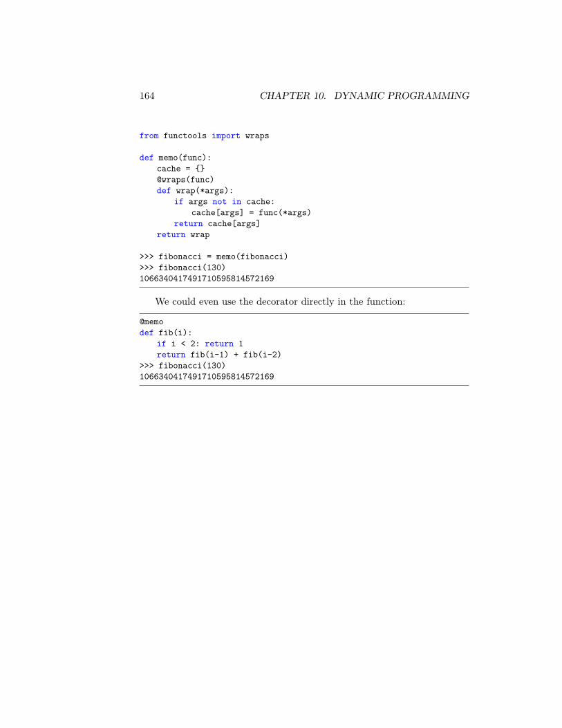
164 CHAPTER 10. DYNAMIC PROGRAMMING
from functools import wraps
def memo(func):cache = {}@wraps(func)def wrap(*args):
if args not in cache:cache[args] = func(*args)
return cache[args]return wrap
>>> fibonacci = memo(fibonacci)>>> fibonacci(130)1066340417491710595814572169
We could even use the decorator directly in the function:
@memodef fib(i):
if i < 2: return 1return fib(i-1) + fib(i-2)
>>> fibonacci(130)1066340417491710595814572169
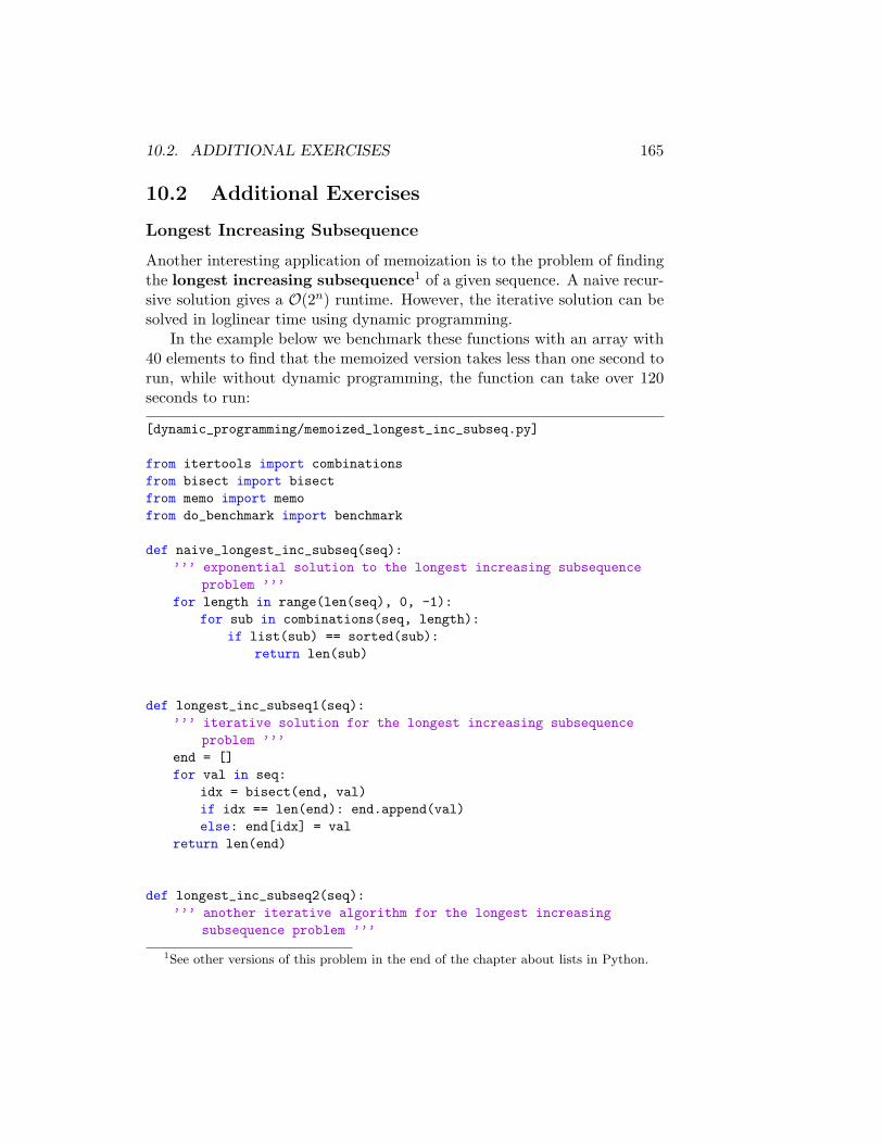
10.2. ADDITIONAL EXERCISES 165
10.2 Additional Exercises
Longest Increasing Subsequence
Another interesting application of memoization is to the problem of findingthe longest increasing subsequence1 of a given sequence. A naive recur-sive solution gives a O(2n) runtime. However, the iterative solution can besolved in loglinear time using dynamic programming.
In the example below we benchmark these functions with an array with40 elements to find that the memoized version takes less than one second torun, while without dynamic programming, the function can take over 120seconds to run:
[dynamic_programming/memoized_longest_inc_subseq.py]
from itertools import combinationsfrom bisect import bisectfrom memo import memofrom do_benchmark import benchmark
def naive_longest_inc_subseq(seq):’’’ exponential solution to the longest increasing subsequence
problem ’’’for length in range(len(seq), 0, -1):
for sub in combinations(seq, length):if list(sub) == sorted(sub):
return len(sub)
def longest_inc_subseq1(seq):’’’ iterative solution for the longest increasing subsequence
problem ’’’end = []for val in seq:
idx = bisect(end, val)if idx == len(end): end.append(val)else: end[idx] = val
return len(end)
def longest_inc_subseq2(seq):’’’ another iterative algorithm for the longest increasing
subsequence problem ’’’
1See other versions of this problem in the end of the chapter about lists in Python.
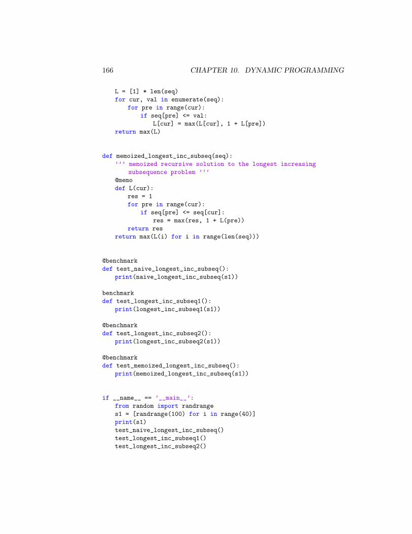
166 CHAPTER 10. DYNAMIC PROGRAMMING
L = [1] * len(seq)for cur, val in enumerate(seq):
for pre in range(cur):if seq[pre] <= val:
L[cur] = max(L[cur], 1 + L[pre])return max(L)
def memoized_longest_inc_subseq(seq):’’’ memoized recursive solution to the longest increasing
subsequence problem ’’’@memodef L(cur):
res = 1for pre in range(cur):
if seq[pre] <= seq[cur]:res = max(res, 1 + L(pre))
return resreturn max(L(i) for i in range(len(seq)))
@benchmarkdef test_naive_longest_inc_subseq():
print(naive_longest_inc_subseq(s1))
benchmarkdef test_longest_inc_subseq1():
print(longest_inc_subseq1(s1))
@benchmarkdef test_longest_inc_subseq2():
print(longest_inc_subseq2(s1))
@benchmarkdef test_memoized_longest_inc_subseq():
print(memoized_longest_inc_subseq(s1))
if __name__ == ’__main__’:from random import randranges1 = [randrange(100) for i in range(40)]print(s1)test_naive_longest_inc_subseq()test_longest_inc_subseq1()test_longest_inc_subseq2()
10.2. ADDITIONAL EXERCISES 167
test_memoized_longest_inc_subseq()

168 CHAPTER 10. DYNAMIC PROGRAMMING
Part III
Climbing Graphs and Trees
169

Chapter 11
Introduction to Graphs
11.1 Basic Definitions
A graph is an abstract network, consisting of nodes (or vertices, V ) connectedby edges (or arcs, E). A graph can be defined as a pair of sets, G = (V,E),where the node set V is any finite set, and the edge set E is a set of nodepairs. For example, some graph can be simply represented by the node setV = {a, b, c, d} and the edge set E = {{a, b}, {b, c}, {c, d}, {d, a}}.
Direction of a Graph
If a graph has no direction, it is referred as undirected. In this case, nodeswith an edge between them are adjacent and adjacent nodes are neighbors.
If the edges have a direction, the graph is directed (digraph). In thiscase, the graph has leaves. The edges are no longer unordered: an edgebetween nodes u and v is now either an edge (u, v) from u to v, or an edge(v, u) from v to u. We can say that in a digraph G, the function E(G) is arelation over V (G).
Subgraphs
A subgraph of G consists of a subset of V and E. A spanning subgraphcontains all the nodes of the original graph.
Completeness of a Graph
If all the nodes in a graph are pairwise adjacent, the graph is called complete.
171

172 CHAPTER 11. INTRODUCTION TO GRAPHS
Degree in a Node
The number of undirected edges incident on a node is called degree. Zero-degree graphs are called isolated. For directed graphs, we can split this num-ber into in-degree (incoming edges/parents) and out-degree/children (outgo-ing edges).
Paths, Walks, and Cycle
A path in G is a subgraph where the edges connect the nodes in a sequence,without revisiting any node. In a directed graph, a path has to follow thedirections of the edges.
A walk is an alternating sequence of nodes and edges that allows nodesand edges to be visited multiple times.
A cycle is like a path except that the last edge links the last node to thefirst.
Length of a Path
The length of a path or walk is the value given by its edge count.
Weight of an Edge
Associating weights with each edge in G gives us a weighted graph. Theweight of a path or cycle is the sum of its edge weights. So, for unweightedgraphs, it is simply the number of edges.
Planar Graphs
A graph that can be drawn on the plane without crossing edges is calledplanar. This graph has regions, which are areas bounded by the edges.TheEuler’s formula for connected planar graphs says that V −E +F = 2, whereV,E, F are the number of nodes, edges, and regions, respectively.
Graph Traversal
A traversal is a walk through all the connected components of a graph. Themain difference between graph traversals is the ordering of the to-do listamong the unvisited nodes that have been discovered.
11.2. THE NEIGHBORHOOD FUNCTION 173
Connected and Strongly Connected Components
An undirected graph is connected if there is a path from every node to everyother node. A directed graph is connected if its underlying undirected graphis connected.
A connected component is a maximal subgraph that is connected. Con-nected components can be found using traversal algorithms such as depth-first searching (DFS) or breath-first searching (BFS), as we will see in fol-lowing chapters.
If there is a path from every node to every other node in a directedgraph, the graph is called strongly connected. A strongly connected compo-nent (SCC) is a maximal subgraph that is strongly connected.
Trees and Forests
A forest is a cycle-free graph. A tree is an acyclic, connected, and directedgraph. A forest consists of one of more trees.
In a tree, any two two nodes are connected by exactly one path. Addingany new edge to it creates a cycle and removing any edge yields unconnectedcomponents.
11.2 The Neighborhood Function
A graph’s neighborhood function, N(V ), is a container (or iterable object) ofall neighbors of V . The most well-known data structures used to representthem are adjacent lists and adjacent matrices.
Adjacent Lists
For each node in an adjacent list, we have access to a list (or set or containeror iterable) of its neighbor. Supposing we have n nodes, each adjacent (orneighbor) list is just a list of such numbers. We place the lists into a mainlist of size n, indexable by the node numbers, where the order is usuallyarbitrary.
Using Sets as Adjacent Lists:
We can use Python’s set type to implement adjacent lists:
>>> a,b,c,d,e,f = range(6) # nodes
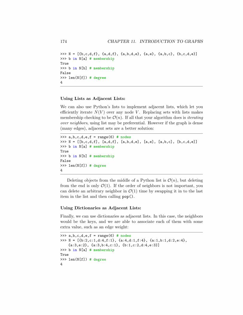
174 CHAPTER 11. INTRODUCTION TO GRAPHS
>>> N = [{b,c,d,f}, {a,d,f}, {a,b,d,e}, {a,e}, {a,b,c}, {b,c,d,e}]>>> b in N[a] # membershipTrue>>> b in N[b] # membershipFalse>>> len(N[f]) # degree4
Using Lists as Adjacent Lists:
We can also use Python’s lists to implement adjacent lists, which let youefficiently iterate N(V ) over any node V . Replacing sets with lists makesmembership checking to be O(n). If all that your algorithm does is iteratingover neighbors, using list may be preferential. However if the graph is dense(many edges), adjacent sets are a better solution:
>>> a,b,c,d,e,f = range(6) # nodes>>> N = [[b,c,d,f], [a,d,f], [a,b,d,e], [a,e], [a,b,c], [b,c,d,e]]>>> b in N[a] # membershipTrue>>> b in N[b] # membershipFalse>>> len(N[f]) # degree4
Deleting objects from the middle of a Python list is O(n), but deletingfrom the end is only O(1). If the order of neighbors is not important, youcan delete an arbitrary neighbor in O(1) time by swapping it in to the lastitem in the list and then calling pop().
Using Dictionaries as Adjacent Lists:
Finally, we can use dictionaries as adjacent lists. In this case, the neighborswould be the keys, and we are able to associate each of them with someextra value, such as an edge weight:
>>> a,b,c,d,e,f = range(6) # nodes>>> N = [{b:2,c:1,d:4,f:1}, {a:4,d:1,f:4}, {a:1,b:1,d:2,e:4},
{a:3,e:2}, {a:3,b:4,c:1}, {b:1,c:2,d:4,e:3}]>>> b in N[a] # membershipTrue>>> len(N[f]) # degree4
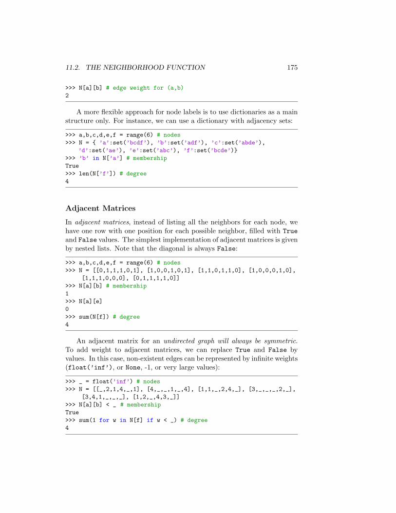
11.2. THE NEIGHBORHOOD FUNCTION 175
>>> N[a][b] # edge weight for (a,b)2
A more flexible approach for node labels is to use dictionaries as a mainstructure only. For instance, we can use a dictionary with adjacency sets:
>>> a,b,c,d,e,f = range(6) # nodes>>> N = { ’a’:set(’bcdf’), ’b’:set(’adf’), ’c’:set(’abde’),
’d’:set(’ae’), ’e’:set(’abc’), ’f’:set(’bcde’)}>>> ’b’ in N[’a’] # membershipTrue>>> len(N[’f’]) # degree4
Adjacent Matrices
In adjacent matrices, instead of listing all the neighbors for each node, wehave one row with one position for each possible neighbor, filled with Trueand False values. The simplest implementation of adjacent matrices is givenby nested lists. Note that the diagonal is always False:
>>> a,b,c,d,e,f = range(6) # nodes>>> N = [[0,1,1,1,0,1], [1,0,0,1,0,1], [1,1,0,1,1,0], [1,0,0,0,1,0],
[1,1,1,0,0,0], [0,1,1,1,1,0]]>>> N[a][b] # membership1>>> N[a][e]0>>> sum(N[f]) # degree4
An adjacent matrix for an undirected graph will always be symmetric.To add weight to adjacent matrices, we can replace True and False byvalues. In this case, non-existent edges can be represented by infinite weights(float(’inf’), or None, -1, or very large values):
>>> _ = float(’inf’) # nodes>>> N = [[_,2,1,4,_,1], [4,_,_,1,_,4], [1,1,_,2,4,_], [3,_,_,_,2,_],
[3,4,1,_,_,_], [1,2,_,4,3,_]]>>> N[a][b] < _ # membershipTrue>>> sum(1 for w in N[f] if w < _) # degree4
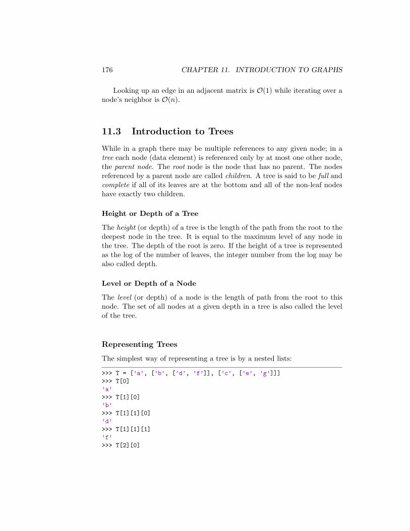
176 CHAPTER 11. INTRODUCTION TO GRAPHS
Looking up an edge in an adjacent matrix is O(1) while iterating over anode’s neighbor is O(n).
11.3 Introduction to Trees
While in a graph there may be multiple references to any given node; in atree each node (data element) is referenced only by at most one other node,the parent node. The root node is the node that has no parent. The nodesreferenced by a parent node are called children. A tree is said to be full andcomplete if all of its leaves are at the bottom and all of the non-leaf nodeshave exactly two children.
Height or Depth of a Tree
The height (or depth) of a tree is the length of the path from the root to thedeepest node in the tree. It is equal to the maximum level of any node inthe tree. The depth of the root is zero. If the height of a tree is representedas the log of the number of leaves, the integer number from the log may bealso called depth.
Level or Depth of a Node
The level (or depth) of a node is the length of path from the root to thisnode. The set of all nodes at a given depth in a tree is also called the levelof the tree.
Representing Trees
The simplest way of representing a tree is by a nested lists:
>>> T = [’a’, [’b’, [’d’, ’f’]], [’c’, [’e’, ’g’]]]>>> T[0]’a’>>> T[1][0]’b’>>> T[1][1][0]’d’>>> T[1][1][1]’f’>>> T[2][0]
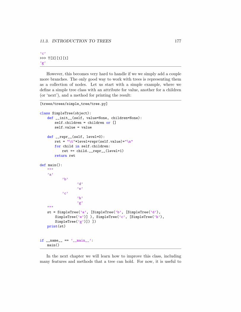
11.3. INTRODUCTION TO TREES 177
’c’>>> T[2][1][1]’g’
However, this becomes very hard to handle if we we simply add a couplemore branches. The only good way to work with trees is representing themas a collection of nodes. Let us start with a simple example, where wedefine a simple tree class with an attribute for value, another for a children(or ‘next’), and a method for printing the result:
[trees/trees/simple_tree/tree.py]
class SimpleTree(object):def __init__(self, value=None, children=None):
self.children = children or []self.value = value
def __repr__(self, level=0):ret = "\t"*level+repr(self.value)+"\n"for child in self.children:
ret += child.__repr__(level+1)return ret
def main():"""’a’
’b’’d’’e’
’c’’h’’g’
"""st = SimpleTree(’a’, [SimpleTree(’b’, [SimpleTree(’d’),
SimpleTree(’e’)] ), SimpleTree(’c’, [SimpleTree(’h’),SimpleTree(’g’)]) ])
print(st)
if __name__ == ’__main__’:main()
In the next chapter we will learn how to improve this class, includingmany features and methods that a tree can hold. For now, it is useful to
178 CHAPTER 11. INTRODUCTION TO GRAPHS
keep in mind that when we are prototyping data structures such as trees, weshould always be able to come up with a flexible class to specify arbitraryattributes in the constructor. The following program implements what isreferred to as a bunch class;, a generic tool that is a specialization of thePython’s dict class and that let you create and set arbitrary attributes onthe fly:
[trees/simple_trees/bunchclass.py]
class BunchClass(dict):def __init__(self, *args, **kwds):
super(BunchClass, self).__init__(*args, **kwds)self.__dict__ = self
def main():’’’ {’right’: {’right’: ’Xander’, ’left’: ’Willow’}, ’left’:
{’right’: ’Angel’, ’left’: ’Buffy’}}’’’bc = BunchClass # notice the absence of ()tree = bc(left = bc(left="Buffy", right="Angel"), right =
bc(left="Willow", right="Xander"))print(tree)
if __name__ == ’__main__’:main()
In the example above, the function’s arguments *args and **kwds canhold an arbitrary number of arguments and an arbitrary number of keywordsarguments, respectively.
Chapter 12
Binary Trees
12.1 Basic Concepts
Binary trees are tree data structures where each node has at most two childnodes: the left and the right. Child nodes may contain references to theirparents. The root of a tree (the ancestor of all nodes) can exist either insideor outside the tree.
Binary trees can be seen as a way of passing an initial number n of tokensdown, meaning that at any point in the tree the sum of all the horizontalnodes will be n. The degree of every node is maximum two. Supposing thatan arbitrary rooted tree has m internal nodes and each internal node hasexactly two children, if the tree has n leaves, the degree of the tree is n− 1:
2m = n + m− 1→ m = n− 1,
i.e a tree with n nodes has exactly n− 1 branches or degree.
12.2 Representing Binary Trees
The simplest (and silliest) way to represent a binary tree is using Python’slists. The following module constructs a list with a root and two emptysublists for the children. To add a left subtree to the root of a tree, weinsert a new list into the second position of the root list. Note that thisalgorithm is not very efficient due to the restrictions that Python’s listshave on inserting and popping in the middle::
179
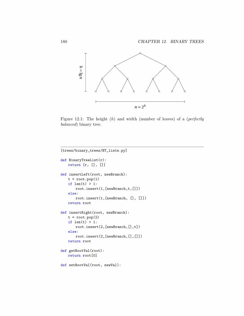
180 CHAPTER 12. BINARY TREES
Figure 12.1: The height (h) and width (number of leaves) of a (perfectlybalanced) binary tree.
[trees/binary_trees/BT_lists.py]
def BinaryTreeList(r):return [r, [], []]
def insertLeft(root, newBranch):t = root.pop(1)if len(t) > 1:
root.insert(1,[newBranch,t,[]])else:
root.insert(1,[newBranch, [], []])return root
def insertRight(root, newBranch):t = root.pop(2)if len(t) > 1:
root.insert(2,[newBranch,[],t])else:
root.insert(2,[newBranch,[],[]])return root
def getRootVal(root):return root[0]
def setRootVal(root, newVal):
12.2. REPRESENTING BINARY TREES 181
root[0] = newVal
def getLeftChild(root):return root[1]
def getRightChild(root):return root[2]
def main():’’’3[5, [4, [], []], []][7, [], [6, [], []]]’’’
r = BinaryTreeList(3)insertLeft(r,4)insertLeft(r,5)insertRight(r,6)insertRight(r,7)print(getRootVal(r))print(getLeftChild(r))print(getRightChild(r))
if __name__ == ’__main__’:main()
However this method is not very practical when we have many branches(or at least it needs many improvements, for example, how it manages thecreation of new lists and how it displays or searches for new elements).
A more natural way to handle binary trees is (again) by representingit as a collection of nodes. A simple node in a binary tree should carryattributes for value and for left and right children, and it can have a methodto identify leaves:
[trees/binary_trees/BT.py]
class BT(object):def __init__(self, value):
self.value = valueself.left = Noneself.right = None
def is_leaf(self):
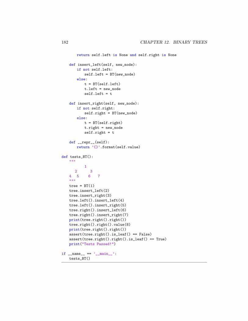
182 CHAPTER 12. BINARY TREES
return self.left is None and self.right is None
def insert_left(self, new_node):if not self.left:
self.left = BT(new_node)else:
t = BT(self.left)t.left = new_nodeself.left = t
def insert_right(self, new_node):if not self.right:
self.right = BT(new_node)else:
t = BT(self.right)t.right = new_nodeself.right = t
def __repr__(self):return ’{}’.format(self.value)
def tests_BT():"""
12 3
4 5 6 7"""tree = BT(1)tree.insert_left(2)tree.insert_right(3)tree.left().insert_left(4)tree.left().insert_right(5)tree.right().insert_left(6)tree.right().insert_right(7)print(tree.right().right())tree.right().right().value(8)print(tree.right().right())assert(tree.right().is_leaf() == False)assert(tree.right().right().is_leaf() == True)print("Tests Passed!")
if __name__ == ’__main__’:tests_BT()
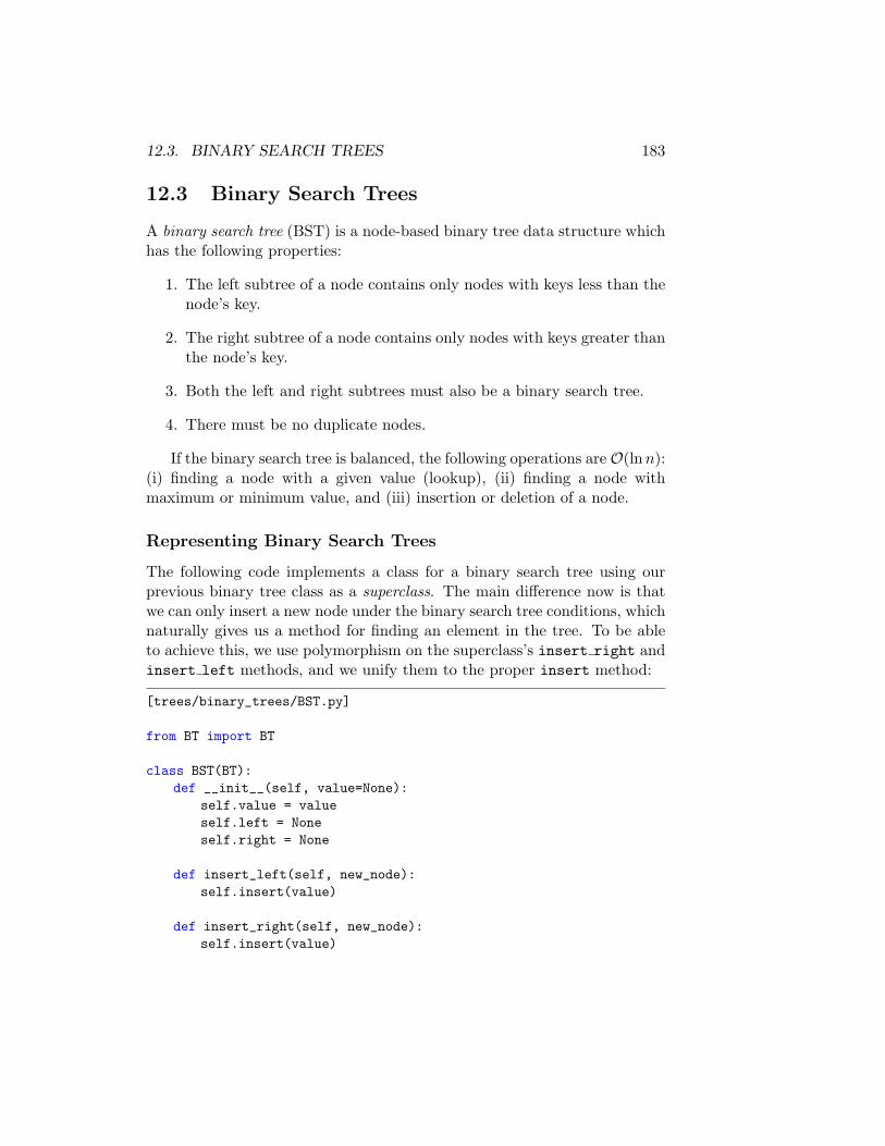
12.3. BINARY SEARCH TREES 183
12.3 Binary Search Trees
A binary search tree (BST) is a node-based binary tree data structure whichhas the following properties:
1. The left subtree of a node contains only nodes with keys less than thenode’s key.
2. The right subtree of a node contains only nodes with keys greater thanthe node’s key.
3. Both the left and right subtrees must also be a binary search tree.
4. There must be no duplicate nodes.
If the binary search tree is balanced, the following operations are O(ln n):(i) finding a node with a given value (lookup), (ii) finding a node withmaximum or minimum value, and (iii) insertion or deletion of a node.
Representing Binary Search Trees
The following code implements a class for a binary search tree using ourprevious binary tree class as a superclass. The main difference now is thatwe can only insert a new node under the binary search tree conditions, whichnaturally gives us a method for finding an element in the tree. To be ableto achieve this, we use polymorphism on the superclass’s insert right andinsert left methods, and we unify them to the proper insert method:
[trees/binary_trees/BST.py]
from BT import BT
class BST(BT):def __init__(self, value=None):
self.value = valueself.left = Noneself.right = None
def insert_left(self, new_node):self.insert(value)
def insert_right(self, new_node):self.insert(value)
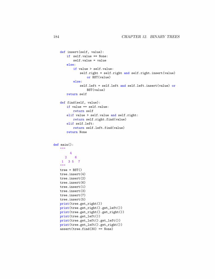
184 CHAPTER 12. BINARY TREES
def insert(self, value):if self.value == None:
self.value = valueelse:
if value > self.value:self.right = self.right and self.right.insert(value)
or BST(value)else:
self.left = self.left and self.left.insert(value) orBST(value)
return self
def find(self, value):if value == self.value:
return selfelif value > self.value and self.right:
return self.right.find(value)elif self.left:
return self.left.find(value)return None
def main():"""
42 6
1 3 5 7"""tree = BST()tree.insert(4)tree.insert(2)tree.insert(6)tree.insert(1)tree.insert(3)tree.insert(7)tree.insert(5)print(tree.get_right())print(tree.get_right().get_left())print(tree.get_right().get_right())print(tree.get_left())print(tree.get_left().get_left())print(tree.get_left().get_right())assert(tree.find(30) == None)
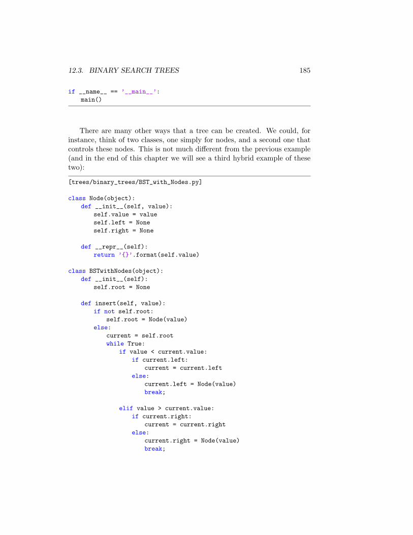
12.3. BINARY SEARCH TREES 185
if __name__ == ’__main__’:main()
There are many other ways that a tree can be created. We could, forinstance, think of two classes, one simply for nodes, and a second one thatcontrols these nodes. This is not much different from the previous example(and in the end of this chapter we will see a third hybrid example of thesetwo):
[trees/binary_trees/BST_with_Nodes.py]
class Node(object):def __init__(self, value):
self.value = valueself.left = Noneself.right = None
def __repr__(self):return ’{}’.format(self.value)
class BSTwithNodes(object):def __init__(self):
self.root = None
def insert(self, value):if not self.root:
self.root = Node(value)else:
current = self.rootwhile True:
if value < current.value:if current.left:
current = current.leftelse:
current.left = Node(value)break;
elif value > current.value:if current.right:
current = current.rightelse:
current.right = Node(value)break;
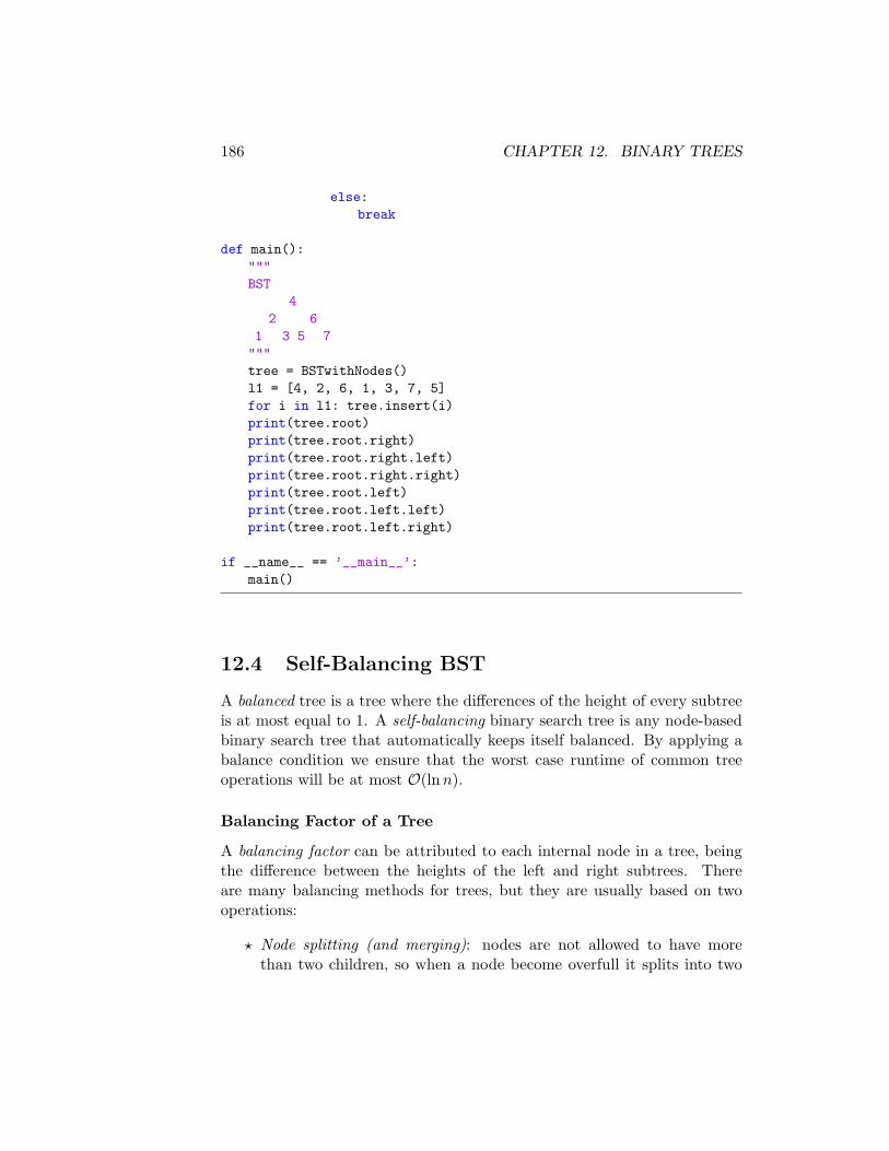
186 CHAPTER 12. BINARY TREES
else:break
def main():"""BST
42 6
1 3 5 7"""tree = BSTwithNodes()l1 = [4, 2, 6, 1, 3, 7, 5]for i in l1: tree.insert(i)print(tree.root)print(tree.root.right)print(tree.root.right.left)print(tree.root.right.right)print(tree.root.left)print(tree.root.left.left)print(tree.root.left.right)
if __name__ == ’__main__’:main()
12.4 Self-Balancing BST
A balanced tree is a tree where the differences of the height of every subtreeis at most equal to 1. A self-balancing binary search tree is any node-basedbinary search tree that automatically keeps itself balanced. By applying abalance condition we ensure that the worst case runtime of common treeoperations will be at most O(ln n).
Balancing Factor of a Tree
A balancing factor can be attributed to each internal node in a tree, beingthe difference between the heights of the left and right subtrees. Thereare many balancing methods for trees, but they are usually based on twooperations:
? Node splitting (and merging): nodes are not allowed to have morethan two children, so when a node become overfull it splits into two
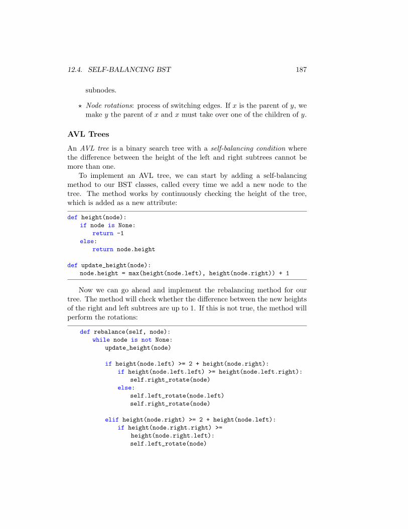
12.4. SELF-BALANCING BST 187
subnodes.
? Node rotations: process of switching edges. If x is the parent of y, wemake y the parent of x and x must take over one of the children of y.
AVL Trees
An AVL tree is a binary search tree with a self-balancing condition wherethe difference between the height of the left and right subtrees cannot bemore than one.
To implement an AVL tree, we can start by adding a self-balancingmethod to our BST classes, called every time we add a new node to thetree. The method works by continuously checking the height of the tree,which is added as a new attribute:
def height(node):if node is None:
return -1else:
return node.height
def update_height(node):node.height = max(height(node.left), height(node.right)) + 1
Now we can go ahead and implement the rebalancing method for ourtree. The method will check whether the difference between the new heightsof the right and left subtrees are up to 1. If this is not true, the method willperform the rotations:
def rebalance(self, node):while node is not None:
update_height(node)
if height(node.left) >= 2 + height(node.right):if height(node.left.left) >= height(node.left.right):
self.right_rotate(node)else:
self.left_rotate(node.left)self.right_rotate(node)
elif height(node.right) >= 2 + height(node.left):if height(node.right.right) >=
height(node.right.left):self.left_rotate(node)
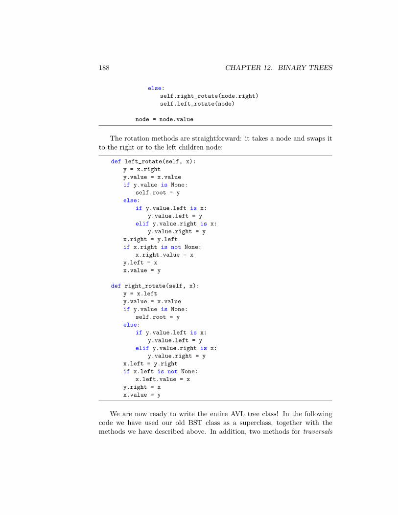
188 CHAPTER 12. BINARY TREES
else:self.right_rotate(node.right)self.left_rotate(node)
node = node.value
The rotation methods are straightforward: it takes a node and swaps itto the right or to the left children node:
def left_rotate(self, x):y = x.righty.value = x.valueif y.value is None:
self.root = yelse:
if y.value.left is x:y.value.left = y
elif y.value.right is x:y.value.right = y
x.right = y.leftif x.right is not None:
x.right.value = xy.left = xx.value = y
def right_rotate(self, x):y = x.lefty.value = x.valueif y.value is None:
self.root = yelse:
if y.value.left is x:y.value.left = y
elif y.value.right is x:y.value.right = y
x.left = y.rightif x.left is not None:
x.left.value = xy.right = xx.value = y
We are now ready to write the entire AVL tree class! In the followingcode we have used our old BST class as a superclass, together with themethods we have described above. In addition, two methods for traversals
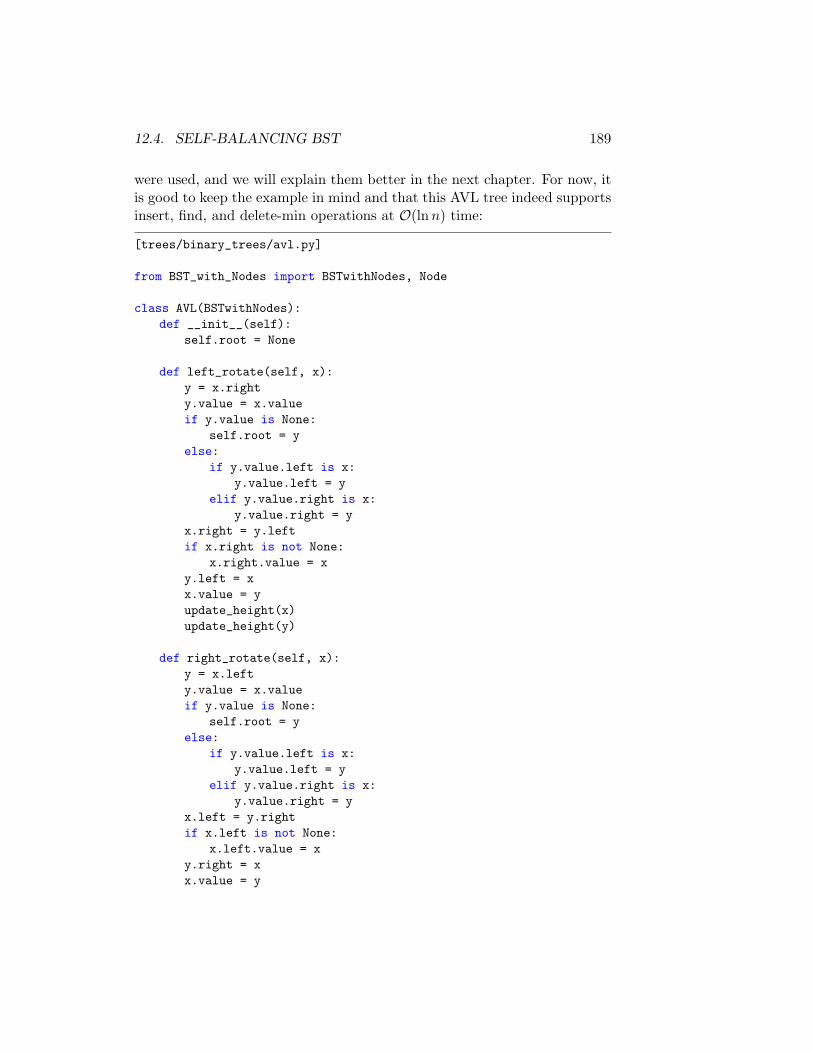
12.4. SELF-BALANCING BST 189
were used, and we will explain them better in the next chapter. For now, itis good to keep the example in mind and that this AVL tree indeed supportsinsert, find, and delete-min operations at O(ln n) time:
[trees/binary_trees/avl.py]
from BST_with_Nodes import BSTwithNodes, Node
class AVL(BSTwithNodes):def __init__(self):
self.root = None
def left_rotate(self, x):y = x.righty.value = x.valueif y.value is None:
self.root = yelse:
if y.value.left is x:y.value.left = y
elif y.value.right is x:y.value.right = y
x.right = y.leftif x.right is not None:
x.right.value = xy.left = xx.value = yupdate_height(x)update_height(y)
def right_rotate(self, x):y = x.lefty.value = x.valueif y.value is None:
self.root = yelse:
if y.value.left is x:y.value.left = y
elif y.value.right is x:y.value.right = y
x.left = y.rightif x.left is not None:
x.left.value = xy.right = xx.value = y
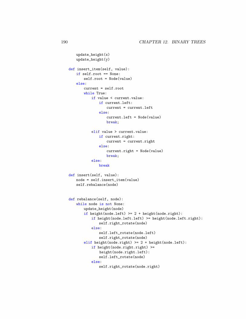
190 CHAPTER 12. BINARY TREES
update_height(x)update_height(y)
def insert_item(self, value):if self.root == None:
self.root = Node(value)else:
current = self.rootwhile True:
if value < current.value:if current.left:
current = current.leftelse:
current.left = Node(value)break;
elif value > current.value:if current.right:
current = current.rightelse:
current.right = Node(value)break;
else:break
def insert(self, value):node = self.insert_item(value)self.rebalance(node)
def rebalance(self, node):while node is not None:
update_height(node)if height(node.left) >= 2 + height(node.right):
if height(node.left.left) >= height(node.left.right):self.right_rotate(node)
else:self.left_rotate(node.left)self.right_rotate(node)
elif height(node.right) >= 2 + height(node.left):if height(node.right.right) >=
height(node.right.left):self.left_rotate(node)
else:self.right_rotate(node.right)
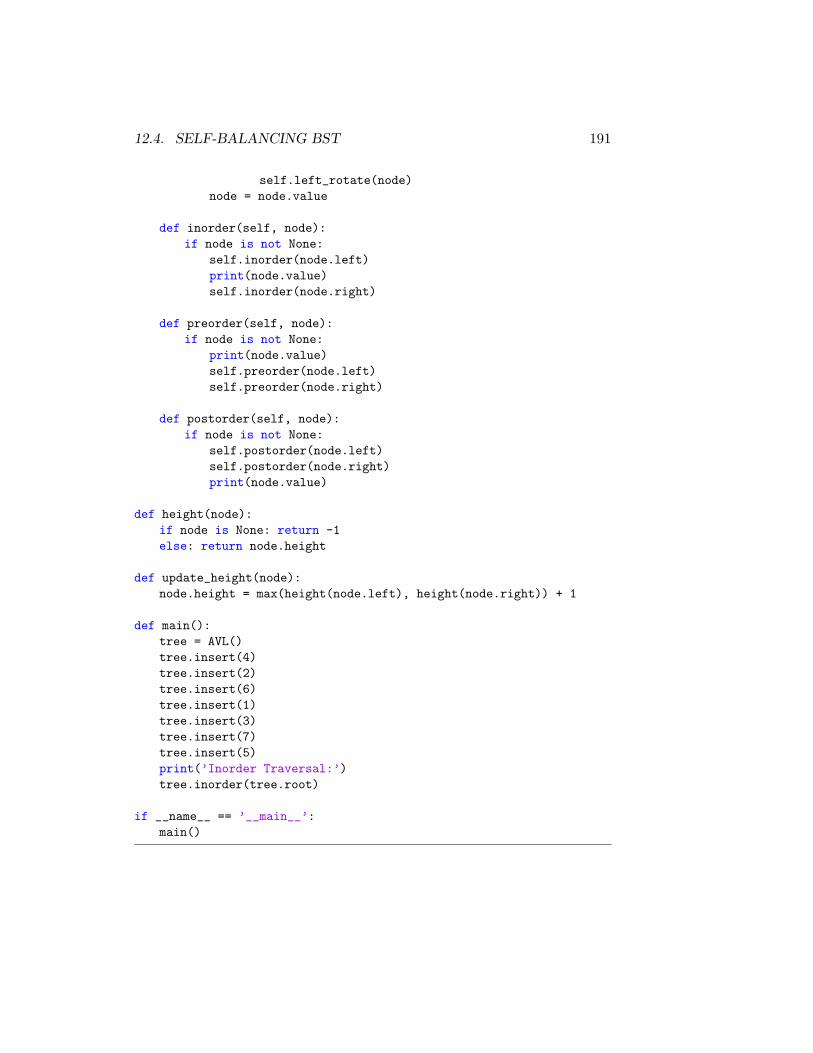
12.4. SELF-BALANCING BST 191
self.left_rotate(node)node = node.value
def inorder(self, node):if node is not None:
self.inorder(node.left)print(node.value)self.inorder(node.right)
def preorder(self, node):if node is not None:
print(node.value)self.preorder(node.left)self.preorder(node.right)
def postorder(self, node):if node is not None:
self.postorder(node.left)self.postorder(node.right)print(node.value)
def height(node):if node is None: return -1else: return node.height
def update_height(node):node.height = max(height(node.left), height(node.right)) + 1
def main():tree = AVL()tree.insert(4)tree.insert(2)tree.insert(6)tree.insert(1)tree.insert(3)tree.insert(7)tree.insert(5)print(’Inorder Traversal:’)tree.inorder(tree.root)
if __name__ == ’__main__’:main()
192 CHAPTER 12. BINARY TREES
Red-black Trees
Red-black trees are an evolution of a binary search trees that aim to keep thetree balanced without affecting the complexity of the primitive operations.This is done by coloring each node in the tree with either red or black andpreserving a set of properties that guarantees that the deepest path in thetree is not longer than twice the shortest one.
Red-black trees have the following properties:
? Every node is colored with either red or black.
? All leaf (nil) nodes are colored with black; if a node’s child is missingthen we will assume that it has a nil child in that place and this nilchild is always colored black.
? Both children of a red node must be black nodes.
? Every path from a node n to a descendent leaf has the same numberof black nodes (not counting node n). We call this number the blackheight of n.
Binary Heaps
Binary heaps are complete balanced binary trees. The heap property makesit easier to maintain the structure, i.e., the balance of the tree. There is noneed to modify a structure of the tree by splitting or rotating nodes in aheap: the only operation will be swapping parent and child nodes.
In a binary heap, the root (the smallest or largest element) is alwaysfound in h[0]. Considering a node at index i:
? the parent index is i−12 ,
? the left child index is 2i + 1,
? the right child index is 2i + 2.
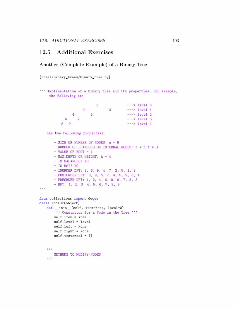
12.5. ADDITIONAL EXERCISES 193
12.5 Additional Exercises
Another (Complete Example) of a Binary Tree
[trees/binary_trees/binary_tree.py]
’’’ Implementation of a binary tree and its properties. For example,the following bt:
1 ---> level 02 3 ---> level 1
4 5 ---> level 26 7 ---> level 3
8 9 ---> level 4
has the following properties:
- SIZE OR NUMBER OF NODES: n = 9- NUMBER OF BRANCHES OR INTERNAL NODES: b = n-1 = 8- VALUE OF ROOT = 1- MAX_DEPTH OR HEIGHT: h = 4- IS BALANCED? NO- IS BST? NO- INORDER DFT: 8, 6, 9, 4, 7, 2, 5, 1, 3- POSTORDER DFT: 8, 9, 6, 7, 4, 5, 2, 3, 1- PREORDER DFT: 1, 2, 4, 6, 8, 9, 7, 5, 3- BFT: 1, 2, 3, 4, 5, 6, 7, 8, 9
’’’
from collections import dequeclass NodeBT(object):
def __init__(self, item=None, level=0):’’’ Construtor for a Node in the Tree ’’’self.item = itemself.level = levelself.left = Noneself.right = Noneself.traversal = []
’’’METHODS TO MODIFY NODES
’’’
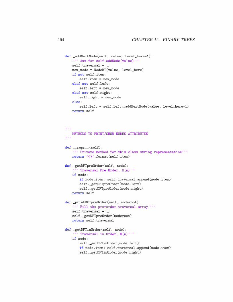
194 CHAPTER 12. BINARY TREES
def _addNextNode(self, value, level_here=1):’’’ Aux for self.addNode(value)’’’self.traversal = []new_node = NodeBT(value, level_here)if not self.item:
self.item = new_nodeelif not self.left:
self.left = new_nodeelif not self.right:
self.right = new_nodeelse:
self.left = self.left._addNextNode(value, level_here+1)return self
’’’METHODS TO PRINT/SHOW NODES ATTRIBUTES
’’’
def __repr__(self):’’’ Private method for this class string representation’’’return ’{}’.format(self.item)
def _getDFTpreOrder(self, node):’’’ Traversal Pre-Order, O(n)’’’if node:
if node.item: self.traversal.append(node.item)self._getDFTpreOrder(node.left)self._getDFTpreOrder(node.right)
return self
def _printDFTpreOrder(self, noderoot):’’’ Fill the pre-order traversal array ’’’self.traversal = []self._getDFTpreOrder(noderoot)return self.traversal
def _getDFTinOrder(self, node):’’’ Traversal in-Order, O(n)’’’if node:
self._getDFTinOrder(node.left)if node.item: self.traversal.append(node.item)self._getDFTinOrder(node.right)
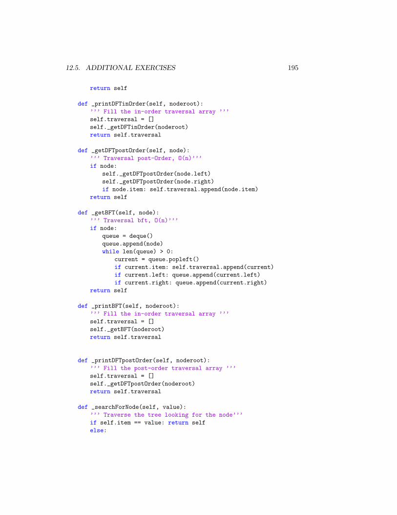
12.5. ADDITIONAL EXERCISES 195
return self
def _printDFTinOrder(self, noderoot):’’’ Fill the in-order traversal array ’’’self.traversal = []self._getDFTinOrder(noderoot)return self.traversal
def _getDFTpostOrder(self, node):’’’ Traversal post-Order, O(n)’’’if node:
self._getDFTpostOrder(node.left)self._getDFTpostOrder(node.right)if node.item: self.traversal.append(node.item)
return self
def _getBFT(self, node):’’’ Traversal bft, O(n)’’’if node:
queue = deque()queue.append(node)while len(queue) > 0:
current = queue.popleft()if current.item: self.traversal.append(current)if current.left: queue.append(current.left)if current.right: queue.append(current.right)
return self
def _printBFT(self, noderoot):’’’ Fill the in-order traversal array ’’’self.traversal = []self._getBFT(noderoot)return self.traversal
def _printDFTpostOrder(self, noderoot):’’’ Fill the post-order traversal array ’’’self.traversal = []self._getDFTpostOrder(noderoot)return self.traversal
def _searchForNode(self, value):’’’ Traverse the tree looking for the node’’’if self.item == value: return selfelse:
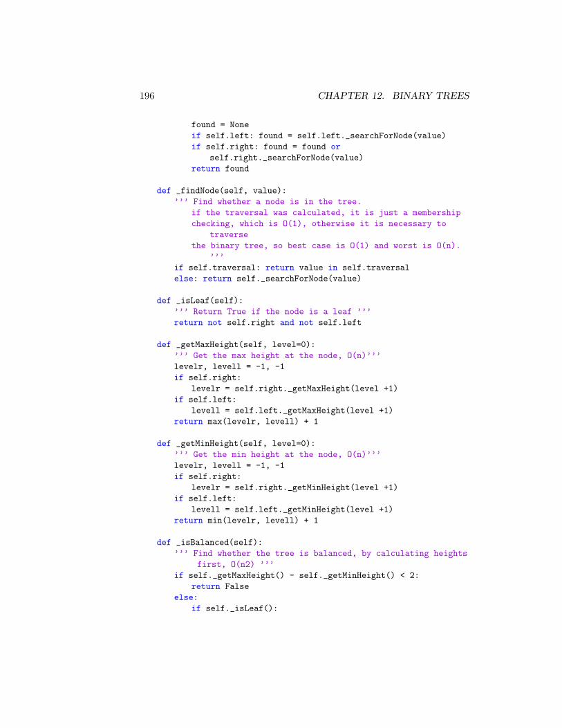
196 CHAPTER 12. BINARY TREES
found = Noneif self.left: found = self.left._searchForNode(value)if self.right: found = found or
self.right._searchForNode(value)return found
def _findNode(self, value):’’’ Find whether a node is in the tree.
if the traversal was calculated, it is just a membershipchecking, which is O(1), otherwise it is necessary to
traversethe binary tree, so best case is O(1) and worst is O(n).
’’’if self.traversal: return value in self.traversalelse: return self._searchForNode(value)
def _isLeaf(self):’’’ Return True if the node is a leaf ’’’return not self.right and not self.left
def _getMaxHeight(self, level=0):’’’ Get the max height at the node, O(n)’’’levelr, levell = -1, -1if self.right:
levelr = self.right._getMaxHeight(level +1)if self.left:
levell = self.left._getMaxHeight(level +1)return max(levelr, levell) + 1
def _getMinHeight(self, level=0):’’’ Get the min height at the node, O(n)’’’levelr, levell = -1, -1if self.right:
levelr = self.right._getMinHeight(level +1)if self.left:
levell = self.left._getMinHeight(level +1)return min(levelr, levell) + 1
def _isBalanced(self):’’’ Find whether the tree is balanced, by calculating heights
first, O(n2) ’’’if self._getMaxHeight() - self._getMinHeight() < 2:
return Falseelse:
if self._isLeaf():
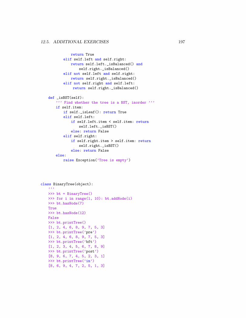
12.5. ADDITIONAL EXERCISES 197
return Trueelif self.left and self.right:
return self.left._isBalanced() andself.right._isBalanced()
elif not self.left and self.right:return self.right._isBalanced()
elif not self.right and self.left:return self.right._isBalanced()
def _isBST(self):’’’ Find whether the tree is a BST, inorder ’’’if self.item:
if self._isLeaf(): return Trueelif self.left:
if self.left.item < self.item: returnself.left._isBST()
else: return Falseelif self.right:
if self.right.item > self.item: returnself.right._isBST()
else: return Falseelse:
raise Exception(’Tree is empty’)
class BinaryTree(object):’’’>>> bt = BinaryTree()>>> for i in range(1, 10): bt.addNode(i)>>> bt.hasNode(7)True>>> bt.hasNode(12)False>>> bt.printTree()[1, 2, 4, 6, 8, 9, 7, 5, 3]>>> bt.printTree(’pre’)[1, 2, 4, 6, 8, 9, 7, 5, 3]>>> bt.printTree(’bft’)[1, 2, 3, 4, 5, 6, 7, 8, 9]>>> bt.printTree(’post’)[8, 9, 6, 7, 4, 5, 2, 3, 1]>>> bt.printTree(’in’)[8, 6, 9, 4, 7, 2, 5, 1, 3]
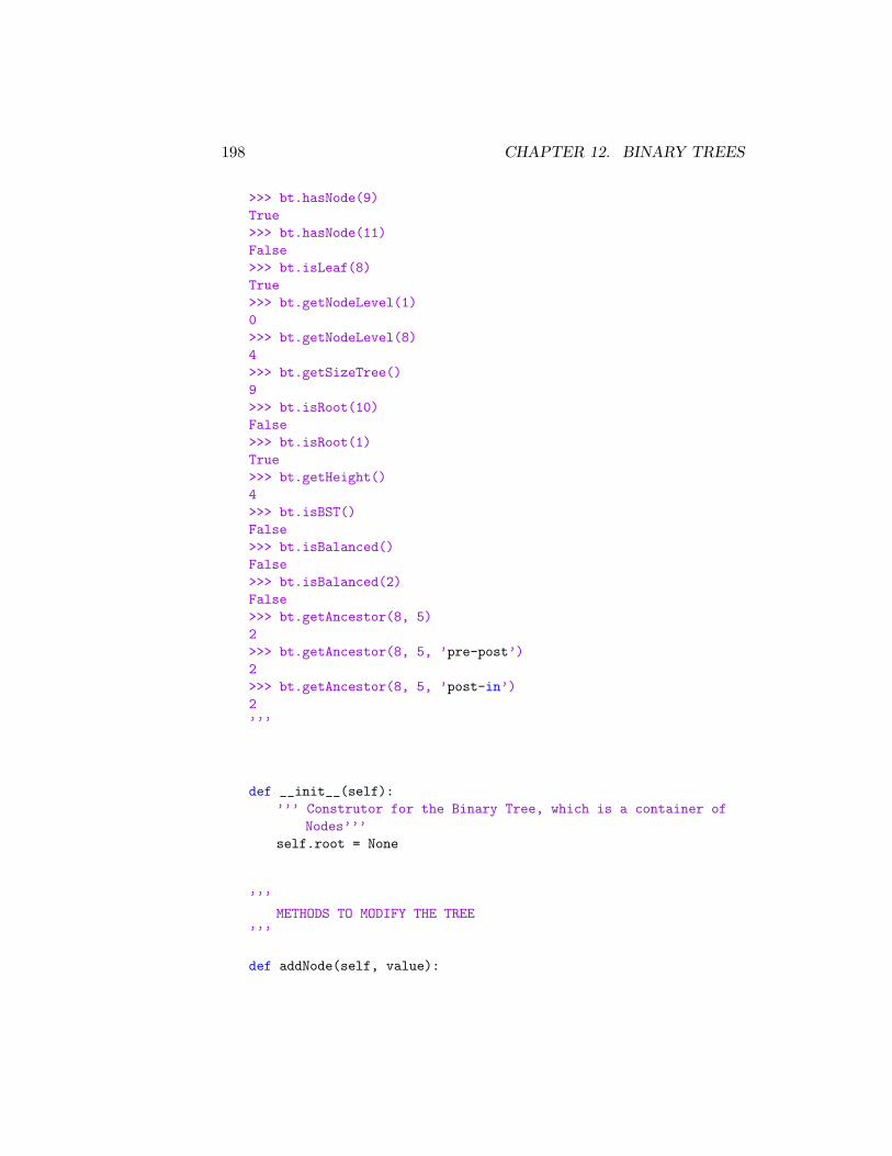
198 CHAPTER 12. BINARY TREES
>>> bt.hasNode(9)True>>> bt.hasNode(11)False>>> bt.isLeaf(8)True>>> bt.getNodeLevel(1)0>>> bt.getNodeLevel(8)4>>> bt.getSizeTree()9>>> bt.isRoot(10)False>>> bt.isRoot(1)True>>> bt.getHeight()4>>> bt.isBST()False>>> bt.isBalanced()False>>> bt.isBalanced(2)False>>> bt.getAncestor(8, 5)2>>> bt.getAncestor(8, 5, ’pre-post’)2>>> bt.getAncestor(8, 5, ’post-in’)2’’’
def __init__(self):’’’ Construtor for the Binary Tree, which is a container of
Nodes’’’self.root = None
’’’METHODS TO MODIFY THE TREE
’’’
def addNode(self, value):
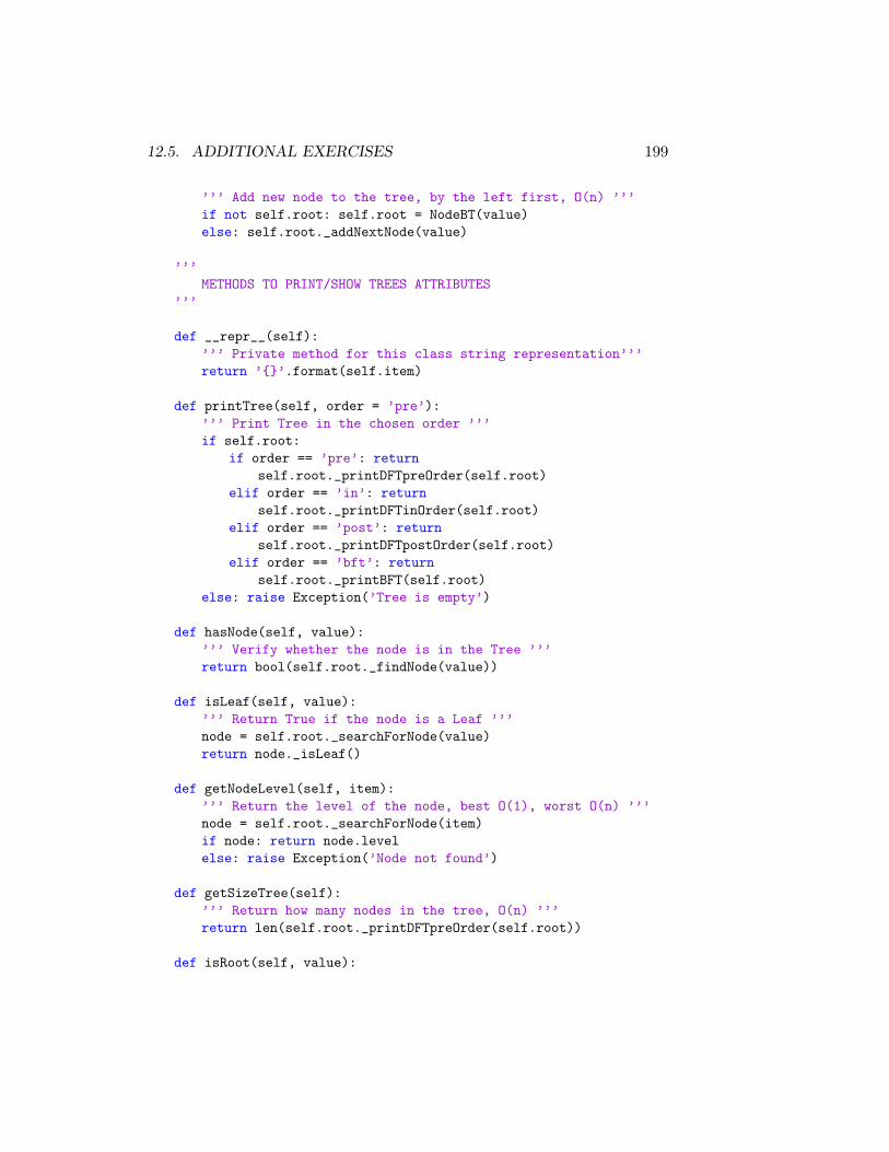
12.5. ADDITIONAL EXERCISES 199
’’’ Add new node to the tree, by the left first, O(n) ’’’if not self.root: self.root = NodeBT(value)else: self.root._addNextNode(value)
’’’METHODS TO PRINT/SHOW TREES ATTRIBUTES
’’’
def __repr__(self):’’’ Private method for this class string representation’’’return ’{}’.format(self.item)
def printTree(self, order = ’pre’):’’’ Print Tree in the chosen order ’’’if self.root:
if order == ’pre’: returnself.root._printDFTpreOrder(self.root)
elif order == ’in’: returnself.root._printDFTinOrder(self.root)
elif order == ’post’: returnself.root._printDFTpostOrder(self.root)
elif order == ’bft’: returnself.root._printBFT(self.root)
else: raise Exception(’Tree is empty’)
def hasNode(self, value):’’’ Verify whether the node is in the Tree ’’’return bool(self.root._findNode(value))
def isLeaf(self, value):’’’ Return True if the node is a Leaf ’’’node = self.root._searchForNode(value)return node._isLeaf()
def getNodeLevel(self, item):’’’ Return the level of the node, best O(1), worst O(n) ’’’node = self.root._searchForNode(item)if node: return node.levelelse: raise Exception(’Node not found’)
def getSizeTree(self):’’’ Return how many nodes in the tree, O(n) ’’’return len(self.root._printDFTpreOrder(self.root))
def isRoot(self, value):
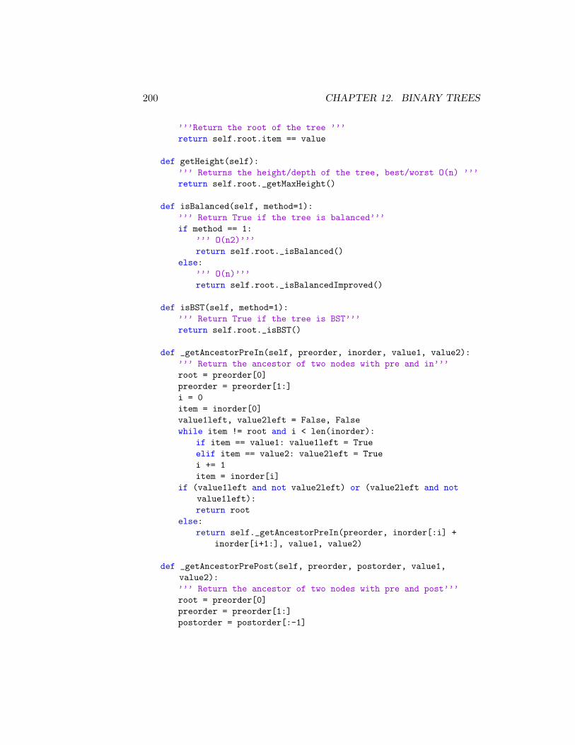
200 CHAPTER 12. BINARY TREES
’’’Return the root of the tree ’’’return self.root.item == value
def getHeight(self):’’’ Returns the height/depth of the tree, best/worst O(n) ’’’return self.root._getMaxHeight()
def isBalanced(self, method=1):’’’ Return True if the tree is balanced’’’if method == 1:
’’’ O(n2)’’’return self.root._isBalanced()
else:’’’ O(n)’’’return self.root._isBalancedImproved()
def isBST(self, method=1):’’’ Return True if the tree is BST’’’return self.root._isBST()
def _getAncestorPreIn(self, preorder, inorder, value1, value2):’’’ Return the ancestor of two nodes with pre and in’’’root = preorder[0]preorder = preorder[1:]i = 0item = inorder[0]value1left, value2left = False, Falsewhile item != root and i < len(inorder):
if item == value1: value1left = Trueelif item == value2: value2left = Truei += 1item = inorder[i]
if (value1left and not value2left) or (value2left and notvalue1left):return root
else:return self._getAncestorPreIn(preorder, inorder[:i] +
inorder[i+1:], value1, value2)
def _getAncestorPrePost(self, preorder, postorder, value1,value2):’’’ Return the ancestor of two nodes with pre and post’’’root = preorder[0]preorder = preorder[1:]postorder = postorder[:-1]
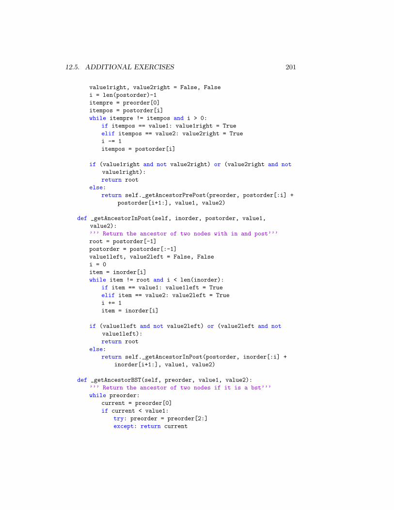
12.5. ADDITIONAL EXERCISES 201
value1right, value2right = False, Falsei = len(postorder)-1itempre = preorder[0]itempos = postorder[i]while itempre != itempos and i > 0:
if itempos == value1: value1right = Trueelif itempos == value2: value2right = Truei -= 1itempos = postorder[i]
if (value1right and not value2right) or (value2right and notvalue1right):return root
else:return self._getAncestorPrePost(preorder, postorder[:i] +
postorder[i+1:], value1, value2)
def _getAncestorInPost(self, inorder, postorder, value1,value2):’’’ Return the ancestor of two nodes with in and post’’’root = postorder[-1]postorder = postorder[:-1]value1left, value2left = False, Falsei = 0item = inorder[i]while item != root and i < len(inorder):
if item == value1: value1left = Trueelif item == value2: value2left = Truei += 1item = inorder[i]
if (value1left and not value2left) or (value2left and notvalue1left):return root
else:return self._getAncestorInPost(postorder, inorder[:i] +
inorder[i+1:], value1, value2)
def _getAncestorBST(self, preorder, value1, value2):’’’ Return the ancestor of two nodes if it is a bst’’’while preorder:
current = preorder[0]if current < value1:
try: preorder = preorder[2:]except: return current
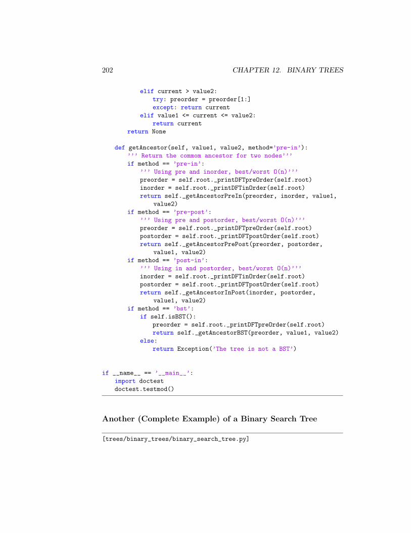
202 CHAPTER 12. BINARY TREES
elif current > value2:try: preorder = preorder[1:]except: return current
elif value1 <= current <= value2:return current
return None
def getAncestor(self, value1, value2, method=’pre-in’):’’’ Return the commom ancestor for two nodes’’’if method == ’pre-in’:
’’’ Using pre and inorder, best/worst O(n)’’’preorder = self.root._printDFTpreOrder(self.root)inorder = self.root._printDFTinOrder(self.root)return self._getAncestorPreIn(preorder, inorder, value1,
value2)if method == ’pre-post’:
’’’ Using pre and postorder, best/worst O(n)’’’preorder = self.root._printDFTpreOrder(self.root)postorder = self.root._printDFTpostOrder(self.root)return self._getAncestorPrePost(preorder, postorder,
value1, value2)if method == ’post-in’:
’’’ Using in and postorder, best/worst O(n)’’’inorder = self.root._printDFTinOrder(self.root)postorder = self.root._printDFTpostOrder(self.root)return self._getAncestorInPost(inorder, postorder,
value1, value2)if method == ’bst’:
if self.isBST():preorder = self.root._printDFTpreOrder(self.root)return self._getAncestorBST(preorder, value1, value2)
else:return Exception(’The tree is not a BST’)
if __name__ == ’__main__’:import doctestdoctest.testmod()
Another (Complete Example) of a Binary Search Tree
[trees/binary_trees/binary_search_tree.py]
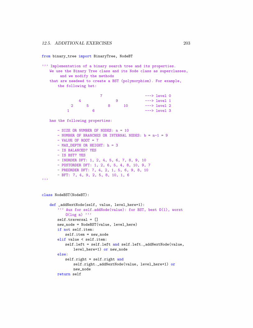
12.5. ADDITIONAL EXERCISES 203
from binary_tree import BinaryTree, NodeBT
’’’ Implementation of a binary search tree and its properties.We use the Binary Tree class and its Node class as superclasses,
and we modify the methodsthat are needeed to create a BST (polymorphism). For example,
the following bst:
7 ---> level 04 9 ---> level 1
2 5 8 10 ---> level 21 6 ---> level 3
has the following properties:
- SIZE OR NUMBER OF NODES: n = 10- NUMBER OF BRANCHES OR INTERNAL NODES: b = n-1 = 9- VALUE OF ROOT = 7- MAX_DEPTH OR HEIGHT: h = 3- IS BALANCED? YES- IS BST? YES- INORDER DFT: 1, 2, 4, 5, 6, 7, 8, 9, 10- POSTORDER DFT: 1, 2, 6, 5, 4, 8, 10, 9, 7- PREORDER DFT: 7, 4, 2, 1, 5, 6, 9, 8, 10- BFT: 7, 4, 9, 2, 5, 8, 10, 1, 6
’’’
class NodeBST(NodeBT):
def _addNextNode(self, value, level_here=1):’’’ Aux for self.addNode(value): for BST, best O(1), worst
O(log n) ’’’self.traversal = []new_node = NodeBST(value, level_here)if not self.item:
self.item = new_nodeelif value < self.item:
self.left = self.left and self.left._addNextNode(value,level_here+1) or new_node
else:self.right = self.right and
self.right._addNextNode(value, level_here+1) ornew_node
return self
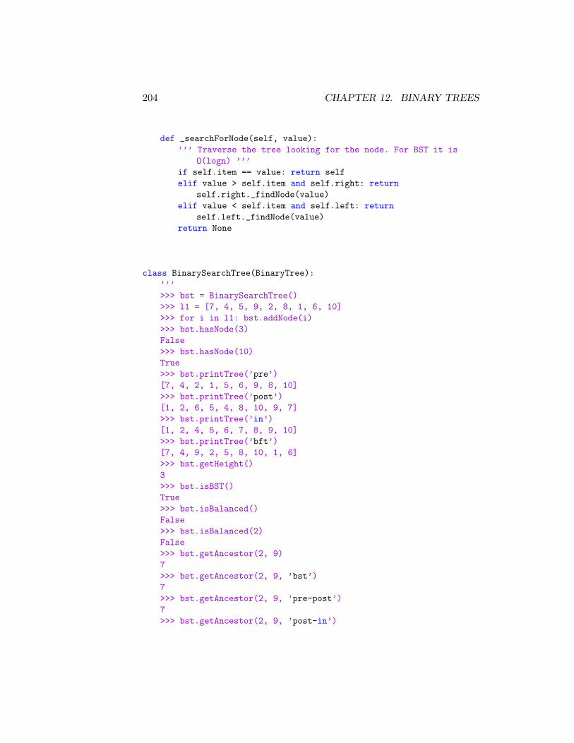
204 CHAPTER 12. BINARY TREES
def _searchForNode(self, value):’’’ Traverse the tree looking for the node. For BST it is
O(logn) ’’’if self.item == value: return selfelif value > self.item and self.right: return
self.right._findNode(value)elif value < self.item and self.left: return
self.left._findNode(value)return None
class BinarySearchTree(BinaryTree):’’’>>> bst = BinarySearchTree()>>> l1 = [7, 4, 5, 9, 2, 8, 1, 6, 10]>>> for i in l1: bst.addNode(i)>>> bst.hasNode(3)False>>> bst.hasNode(10)True>>> bst.printTree(’pre’)[7, 4, 2, 1, 5, 6, 9, 8, 10]>>> bst.printTree(’post’)[1, 2, 6, 5, 4, 8, 10, 9, 7]>>> bst.printTree(’in’)[1, 2, 4, 5, 6, 7, 8, 9, 10]>>> bst.printTree(’bft’)[7, 4, 9, 2, 5, 8, 10, 1, 6]>>> bst.getHeight()3>>> bst.isBST()True>>> bst.isBalanced()False>>> bst.isBalanced(2)False>>> bst.getAncestor(2, 9)7>>> bst.getAncestor(2, 9, ’bst’)7>>> bst.getAncestor(2, 9, ’pre-post’)7>>> bst.getAncestor(2, 9, ’post-in’)
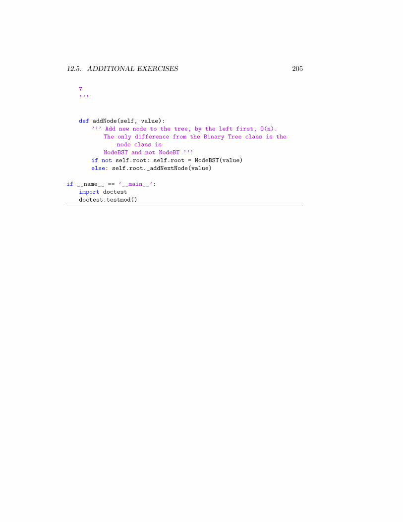
12.5. ADDITIONAL EXERCISES 205
7’’’
def addNode(self, value):’’’ Add new node to the tree, by the left first, O(n).
The only difference from the Binary Tree class is thenode class is
NodeBST and not NodeBT ’’’if not self.root: self.root = NodeBST(value)else: self.root._addNextNode(value)
if __name__ == ’__main__’:import doctestdoctest.testmod()

206 CHAPTER 12. BINARY TREES
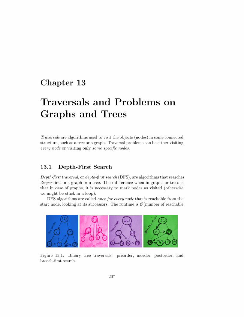
Chapter 13
Traversals and Problems onGraphs and Trees
Traversals are algorithms used to visit the objects (nodes) in some connectedstructure, such as a tree or a graph. Traversal problems can be either visitingevery node or visiting only some specific nodes.
13.1 Depth-First Search
Depth-first traversal, or depth-first search (DFS), are algorithms that searchesdeeper first in a graph or a tree. Their difference when in graphs or trees isthat in case of graphs, it is necessary to mark nodes as visited (otherwisewe might be stuck in a loop).
DFS algorithms are called once for every node that is reachable from thestart node, looking at its successors. The runtime is O(number of reachable
Figure 13.1: Binary tree traversals: preorder, inorder, postorder, andbreath-first search.
207
208CHAPTER 13. TRAVERSALS AND PROBLEMS ON GRAPHS AND TREES
nodes + total number of outgoing edges from these nodes) = O(V + E).DFSs are usually implemented using LIFO structure such as stacks to keeptrack of the discovered nodes, and they can be divided in three differentstrategies:
Preorder: Visit a node before traversing subtrees (root → left → right):
def preorder(root):if root != 0:
yield root.valuepreorder(root.left)preorder(root.right)
Postorder: Visit a node after traversing all subtrees (left→ right→ root):
def postorder(root):if root != 0:
postorder(root.left)postorder(root.right)yield root.value
Inorder: Visit a node after traversing its left subtree but before the rightsubtree (left → root → right):
def inorder(root):if root != 0:
inorder(root.left)yield root.valueinorder(root.right)
13.2 Breadth-First Search
Breadth-first traversal, or breath-first search (BFS), are algorithms that yieldsthe values of all nodes of a particular depth before going to any deeper node.
Problems that use BFS usually ask to find the fewest number of steps(or the shortest path) needed to reach a certain end point from the starting
13.3. REPRESENTING TREE TRAVERSALS 209
point. Traditionally, BFSs are implemented using a list to store the valuesof the visited nodes and then a FIFO queue to store those nodes that haveyet to be visited. The total runtime is also O(V + E).
13.3 Representing Tree Traversals
There are many ways we could write traversals. In the following code weuse the “BST with nodes” class, defined in the last chapter, to implementeach of the traversal algorithms. For the DFS cases, we have also tested twodifferent methods:
[trees/traversals/BST_with_Nodes_traversal.py]
from BST_with_Nodes import BSTwithNodes, Node
class BSTTraversal(BSTwithNodes):def __init__(self):
self.root = Noneself.nodes_BFS = []self.nodes_DFS_pre = []self.nodes_DFS_post = []self.nodes_DFS_in = []
def BFS(self):self.root.level = 0queue = [self.root]current_level = self.root.level
while len(queue) > 0:current_node = queue.pop(0)if current_node.level > current_level:
current_level += 1self.nodes_BFS.append(current_node.value)
if current_node.left:current_node.left.level = current_level + 1queue.append(current_node.left)
if current_node.right:current_node.right.level = current_level + 1queue.append(current_node.right)
210CHAPTER 13. TRAVERSALS AND PROBLEMS ON GRAPHS AND TREES
return self.nodes_BFS
def DFS_inorder(self, node):if node is not None:
self.DFS_inorder(node.left)self.nodes_DFS_in.append(node.value)self.DFS_inorder(node.right)
return self.nodes_DFS_in
def DFS_preorder(self, node):if node is not None:
self.nodes_DFS_pre.append(node.value)self.DFS_preorder(node.left)self.DFS_preorder(node.right)
return self.nodes_DFS_pre
def DFS_postorder(self, node):if node is not None:
self.DFS_postorder(node.left)self.DFS_postorder(node.right)self.nodes_DFS_post.append(node.value)
return self.nodes_DFS_post
def main():tree = BSTTraversal()l1 = [10, 5, 15, 1, 6, 11, 50]for i in l1: tree.insert(i)
print(’Breadth-First Traversal: ’, tree.BFS())print(’Inorder Traversal: ’, tree.DFS_inorder(tree.root))print(’Preorder Traversal: ’, tree.DFS_preorder(tree.root))print(’Postorder Traversal: ’, tree.DFS_postorder(tree.root))
if __name__ == ’__main__’:main()
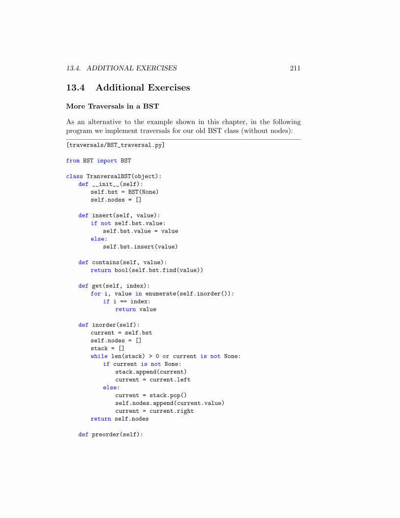
13.4. ADDITIONAL EXERCISES 211
13.4 Additional Exercises
More Traversals in a BST
As an alternative to the example shown in this chapter, in the followingprogram we implement traversals for our old BST class (without nodes):
[traversals/BST_traversal.py]
from BST import BST
class TranversalBST(object):def __init__(self):
self.bst = BST(None)self.nodes = []
def insert(self, value):if not self.bst.value:
self.bst.value = valueelse:
self.bst.insert(value)
def contains(self, value):return bool(self.bst.find(value))
def get(self, index):for i, value in enumerate(self.inorder()):
if i == index:return value
def inorder(self):current = self.bstself.nodes = []stack = []while len(stack) > 0 or current is not None:
if current is not None:stack.append(current)current = current.left
else:current = stack.pop()self.nodes.append(current.value)current = current.right
return self.nodes
def preorder(self):
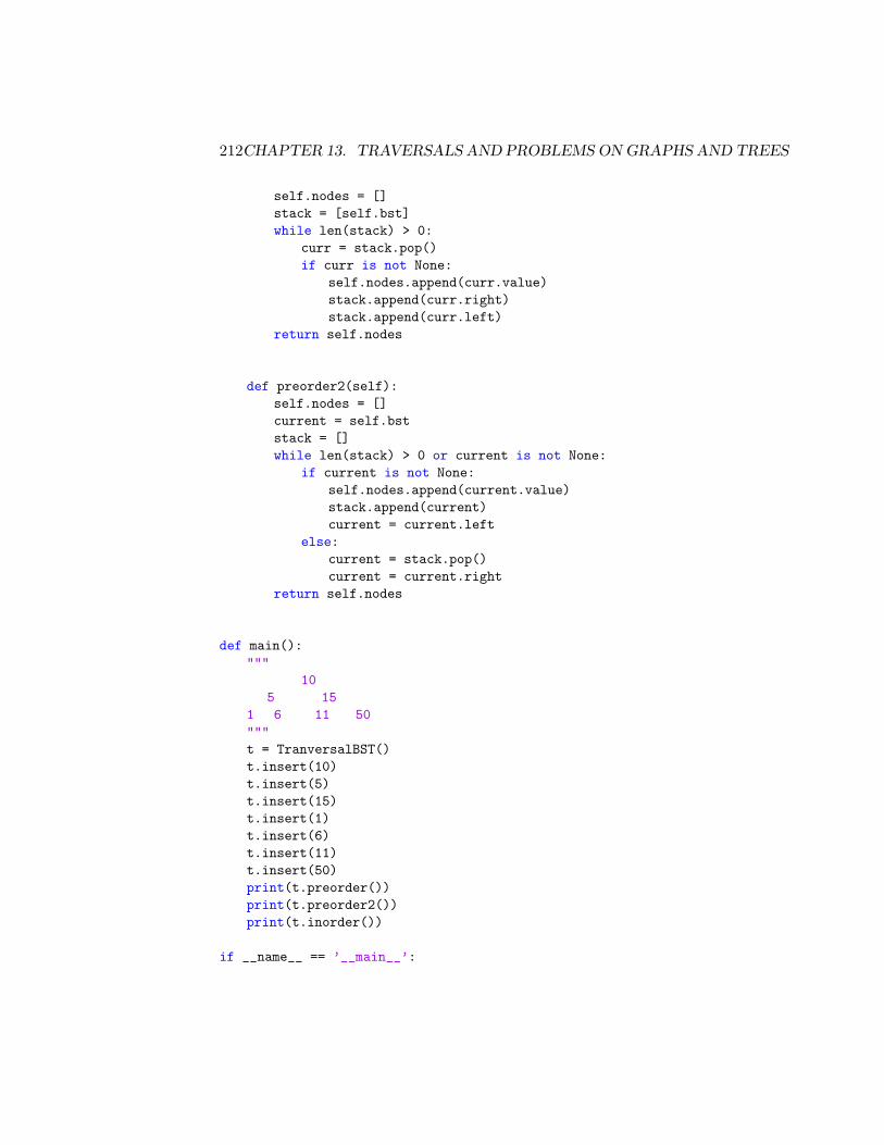
212CHAPTER 13. TRAVERSALS AND PROBLEMS ON GRAPHS AND TREES
self.nodes = []stack = [self.bst]while len(stack) > 0:
curr = stack.pop()if curr is not None:
self.nodes.append(curr.value)stack.append(curr.right)stack.append(curr.left)
return self.nodes
def preorder2(self):self.nodes = []current = self.bststack = []while len(stack) > 0 or current is not None:
if current is not None:self.nodes.append(current.value)stack.append(current)current = current.left
else:current = stack.pop()current = current.right
return self.nodes
def main():"""
105 15
1 6 11 50"""t = TranversalBST()t.insert(10)t.insert(5)t.insert(15)t.insert(1)t.insert(6)t.insert(11)t.insert(50)print(t.preorder())print(t.preorder2())print(t.inorder())
if __name__ == ’__main__’:
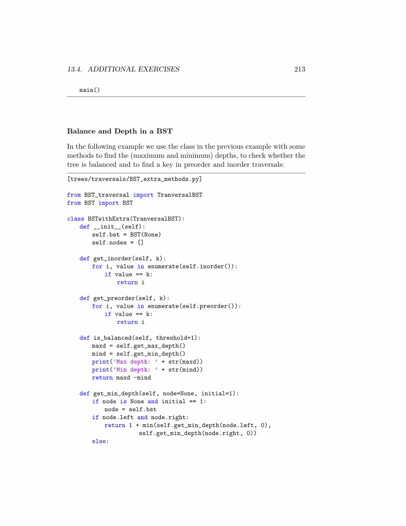
13.4. ADDITIONAL EXERCISES 213
main()
Balance and Depth in a BST
In the following example we use the class in the previous example with somemethods to find the (maximum and minimum) depths, to check whether thetree is balanced and to find a key in preorder and inorder traversals:
[trees/traversals/BST_extra_methods.py]
from BST_traversal import TranversalBSTfrom BST import BST
class BSTwithExtra(TranversalBST):def __init__(self):
self.bst = BST(None)self.nodes = []
def get_inorder(self, k):for i, value in enumerate(self.inorder()):
if value == k:return i
def get_preorder(self, k):for i, value in enumerate(self.preorder()):
if value == k:return i
def is_balanced(self, threshold=1):maxd = self.get_max_depth()mind = self.get_min_depth()print(’Max depth: ’ + str(maxd))print(’Min depth: ’ + str(mind))return maxd -mind
def get_min_depth(self, node=None, initial=1):if node is None and initial == 1:
node = self.bstif node.left and node.right:
return 1 + min(self.get_min_depth(node.left, 0),self.get_min_depth(node.right, 0))
else:
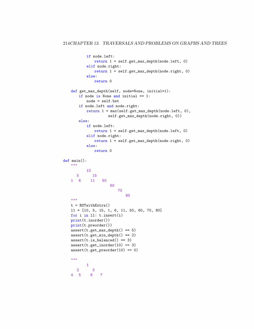
214CHAPTER 13. TRAVERSALS AND PROBLEMS ON GRAPHS AND TREES
if node.left:return 1 + self.get_max_depth(node.left, 0)
elif node.right:return 1 + self.get_max_depth(node.right, 0)
else:return 0
def get_max_depth(self, node=None, initial=1):if node is None and initial == 1:
node = self.bstif node.left and node.right:
return 1 + max(self.get_max_depth(node.left, 0),self.get_max_depth(node.right, 0))
else:if node.left:
return 1 + self.get_max_depth(node.left, 0)elif node.right:
return 1 + self.get_max_depth(node.right, 0)else:
return 0
def main():"""
105 15
1 6 11 5060
7080
"""t = BSTwithExtra()l1 = [10, 5, 15, 1, 6, 11, 50, 60, 70, 80]for i in l1: t.insert(i)print(t.inorder())print(t.preorder())assert(t.get_max_depth() == 5)assert(t.get_min_depth() == 2)assert(t.is_balanced() == 3)assert(t.get_inorder(10) == 3)assert(t.get_preorder(10) == 0)
"""1
2 34 5 6 7
13.4. ADDITIONAL EXERCISES 215
"""t2 = BSTwithExtra()l2 = [1, 2, 3, 4, 5, 6, 7, 8]for i in l2: t2.insert(i)print(t2.inorder())print(t2.preorder())assert(t2.is_balanced() == 0)
print("Tests Passed!")
if __name__ == ’__main__’:main()
Ancestor in a BST
The example bellow finds the lowest level common ancestor of two nodes ina binary search tree:
[trees/traversals/BST_ancestor.py]
from BST_traversal import TranversalBST
def find_ancestor(path, low_value, high_value):’’’ find the lowest ancestor in a BST ’’’while path:
current_value = path[0]if current_value < low_value:
try:path = path[2:]
except:return current_value
elif current_value > high_value:try:
path = path[1:]except:
return current_valueelif low_value <= current_value <= high_value:
return current_valuereturn None
def test_find_ancestor():"""
216CHAPTER 13. TRAVERSALS AND PROBLEMS ON GRAPHS AND TREES
105 15
1 6 11 50"""t = TranversalBST()l1 = [10, 5, 15, 1, 6, 11, 50]for i in l1: t.insert(i)path = t.preorder()assert(find_ancestor(path, 1, 6) == 5)assert(find_ancestor(path, 1, 11) == 10)assert(find_ancestor(path, 11, 50) == 15)assert(find_ancestor(path, 5, 15) == 10)
print("Tests passsed!")
if __name__ == ’__main__’:test_find_ancestor()
Bibliography
Websites:
[Interactive Python] http://interactivepython.org
[Python’s Official Documentation] http://docs.python.org/3/tutorial/
[Google Style Guide] http://google-styleguide.code.com/svn/trunk/pyguide.html
[My free GIT Repository] https://bitbucket.org/steinkirch/exercises-in-python:All the examples in this book are there, plus many exercises that I havenot included here.
[XKCD Comics] https://xkcd.com/
[Big-O Sheet] http://bigocheatsheet.com/
Books:
[A nice Book for Software Eng. Interviews] Cracking the Coding In-terview, Gayle Laakmann McDowell, 2013
217
218 BIBLIOGRAPHY
[A nice Python 3 Book] Programming in Python 3: A Complete Intro-duction to the Python 3.1 Language, Mark Summerfield, 2011
[A nice Python Book] Learn Python The Hard Way, Zed A. Shaw, 2010
[A nice Algorithms Book] Mastering Basic Algorithms in the PythonLanguage, Magnus Lie Hetland, 2010
[Another nice Algorithms Book] The Algorithm Design Manual, S.S.Skiena, 2008
[Another nice Python Book] Python 3 Object Oriented Programming,Dusty Phillips, 2010
[Another nice guide for Software Eng. Interviews] ProgrammingPearls, Jon Bentley, 1986