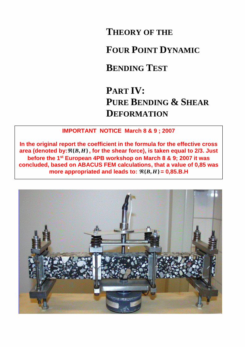
THEORY OF THE

FOUR POINT DYNAMIC

BENDING TEST

PART IV:

PURE BENDING & SHEAR

DEFORMATION

IMPORTANT NOTICE March 8 & 9 ; 2007

In the original report the coefficient in the formula for the effective cross area (denoted by: B H{ , } , for the shear force), is taken equal to 2/3. Just

before the 1st European 4PB workshop on March 8 & 9; 2007 it was concluded, based on ABACUS FEM calculations, that a value of 0,85 was

more appropriated and leads to: B H{ , } = 0,85.B.H

THEORY OF THE

FOUR POINT DYNAMIC

BENDING TEST

PART IV: PURE BENDING & SHEAR DEFORMATION

AUTHOR: A.C. PRONK

DATE: 1ST CONCEPT SEPTEMBER 2002 FINISHED MAY 2007

Abstract

This report deals with the commonly neglected influences of shear forces on the

measured deflections in the dynamic four point bending test. The report forms the

fourth part in the series of reports on the “Theory of the Four Point Dynamic Bending

Test”. It is world wide adopted that for a bending test in which the ratio of the

(effective) length or span of the beam and the height of the beam is above a factor 8

the deflection due to shear forces can be neglected. This judgement is based on a

comparison between the differential equations for pseudo-static bending tests. In this

report the complete analytical solutions are derived for cyclic bending test conditions.

It is shown that the deflection part due to shear forces is around 5% of the total

deflection. For a good understanding of the theory it is advised to use Part I and II of

the series on the Theory of the Four Point Bending Test next to this report.

Contents

1. GENERAL BENDING THEORY OF A RECTANGULAR BEAM

2. BOUNDARY CONDITIONS

3. DEVELOPMENT OF Q{x,t} IN SERIES OF SINES (orthogonal functions)

4. DEVELOPMENT OF THE OTHER MASS FORCES IN SERIES

5. FUNCTION FORMULATION FOR Vb and Vs

6. THEORETICAL SOLUTION WHEN NO EXTRA MASSES ARE PRESENT

7. SOLUTION FOR THE PSEUDO-STATIC CASE

8. HOW TO INCORPERATE EXTRA MOVING MASSES.

ANNEX I “Development in Sine or Cosine Series”

ANNEX II “The series development for the deflection due to shear”

DISCLAIMER

This working paper is issued to give those interested an opportunity to acquaint themselves with progress in this particular

field of research. It must be stressed that the opinions expressed in this working paper do not necessarily reflect the official

point of view or the policy of the director-general of the Rijkswaterstaat. The information given in this working paper should

therefore be treated with caution in case the conclusions are revised in the course of further research or in some other way.

The Kingdom of the Netherlands takes no responsibility for any losses incurred as a result of using the information contained

in this working paper.

Pure Bending & Shear Deformation

1. GENERAL BENDING THEORY OF A RECTANGULAR BEAM

The bending theory for a rectangular beam is given by two differential equations:

02

3

2

2

DMx

t,xVbxt

.I.

t,xQDx

t,xVst,xVbt

.H.B.

[1a,b]

In which: Vb = Deflection due to pure bending

Vs = Deflection due to shear forces

B = Width of beam

H = Height of beam

Ltot = Total length of beam

L = Effective length = distance between the two outer supports

A = Distance between outer and inner supports

= Distance from x=0 to first outer support (=(Lt-L)/2)

Fo = Applied force at the two inner supports (clamps)

I = Moment of the beam (B.H3/12)

D = Shear force

M = Bending moment

Q = Force distribution along the beam

E = Stiffness modulus of beam

G = Shear modulus (E/(2(1+)))

= Density

= Poisson ratio

The moment M is related to the deflection Vb by:

t,xVbx

.I.EM2

2

[2]

And the shear force D is related to the shear deflection Vs by:

AreaCross Effective HB, with

t,xVs

x.H,B.GD [3]

Integration of equation [1b] over x leads to a relationship between the shear deflection Vs

and the bending deflection Vb:

tt,xVb

x.Et,xVb

t..

H,B.G

It,xVs

2

2

2

2

[4]

in which t is a yet unknown function in the time t only.

Differentiation of equation [1b] and adding to equation [1a] leads to a relationship between

the total deflection Vt and the bending deflection Vb :

t,xQt,xVbx

.I.Et,xVbxt

.I.t,xVtt

.H.B.

4

4

2

2

2

2

2

2

[5]

Using equation [4] in equation [5] leads to the desired relationship between the bending

deflection Vb and the force distribution Q:

t,xQt

dt

dt,xVb

xt.Et,xVb

t..

H,B.G

I.H.B.

t,xVbx

.I.Et,xVbxt

I.t,xVbt

.H.B.

2

2

2

2

2

2

4

4

4

4

2

2

2

2

2

2

[6]

Elimination of Vb by substituting equation 1a into equation 1b after two derivations with

respect to the time t leads to:

tdt

dt,xVs

t.H,BG

t,xVsxt

H,B.Gt,xVst

.H.B.t,xQdt

d

H.B.

I.

t,xVsx

.H,B.Gt,xVsxt

.H.B.t,xQdx

d.

H.B.

I.E

2

2

2

2

2

2

2

2

4

4

2

2

4

4

2

2

2

2

2

2

[7]

From equations [6] and [7] it is clear that both Vb and Vs contain a function which only

depends on the time: Vb+f{t} and Vs+g{t}.

Rearrangement of the two basic differential equations leads to:

}t,x{Q}t,x{Vbtx

.I.E}t,x{Vbt

.I..}H,B{.G

H.B.

}t,x{Vbtx

.I.}t,x{Vbt

.H.B.}t,x{Vbx

.I.E

22

4

4

4

22

4

2

2

4

4

[8]

}t,x{Q.x

.Et

..H.B.

I}t,x{Vs

t}.H,B{.G

}t,x{Vs.x

.Et

.x

.H.B.

}H,B{.G

t.I

2

2

2

2

2

2

2

2

2

2

2

2

2

2

[9]

After estimations for the several coefficients the following two (approximated) differential

equations for the pure bending deflection Vb and the shear deflection Vs can be established

(see reference 1):

}t,x{Q}t,x{Vsx

}.H,B{.G

}t,x{Q}t,x{Vbt

.H.B.}t,x{Vbx

.I.E

2

2

2

2

4

4

[10a,b]

Equations 10a and 10b are used for the forward calculation of the deflection Vtot = Vb+Vs if

the other parameters like E, B, H, G, and Q{x,t} are given. Notice that Q{x,t} has the

dimension N/m; in equation 10 it is a force per length. The deviation made by the ignoring

the other terms in equations 8 and 9 is negligible. Mark that if extra moving masses are

present, the two differential equations are coupled by an extra term (common force) in

both equations: mass mass mass mass mass mass

mass mass mass

Q x t F x t x M Vt x t xt

M Vb x t Vs x t xt

2

2

2

2

{ , } { , }. { } . { , }. { }

. { , } { , } . { }

[10c]

This expression has the dimension N/m and acts only at x = xmass and Ltot – xmass and

at x = and Ltot – . See also equation [12] and [13].

Equations 10a and 10b will be solved (the steady state) for a sinusoidal load signal of the

form: eit.

2. BOUNDARY CONDITIONS

In case of a four point bending test (4PB) the following boundary conditions are valid for

equal sinusoidal point loads at the two inner clamps and only regarding the steady state

condition:

[11a,b,c]

2

tot 2

tot

tot

At x 0 and L : M{x,t} E.I. Vb x t 0 &x

D{x,t} G. {B,H}. Vs x t 0 [I]x

At x and L - : Vt{x,t} = Vb{x,t} + Vs{x,t} 0 [II]

At x L /2 : x

{ , }

{ , }

Vb x t & Vs x t [III]

x{ , } 0 { , } 0

3. DEVELOPMENT OF Q{x,t} IN SERIES OF SINES (orthogonal functions)

For the solution of the differential equations it is necessarily1 to develop the discrete

position functions for the point loads into series of orthogonal functions. Given the simple

character of the equation a common sinus or cosines series is already sufficient.

The discrete position function for the load distribution Q{x,t} is given by:

t.ω.i

tottot e.LδALδAxδxδ.F

}t,x{Q 0ΔΔΔΔ2

0 [12]

in which {x=a} represents the delta function:

a

a

afdx.xf.ax [13]

In case of only pure bending a series of orthogonal sine functions would be sufficient. At

x=0 and x=Ltot the moment M (:: 2/ x2) has to be zero, which in case of a sine function is

automatically fulfilled: i ti t

n

n tot

xQ x t F x e F Sin n e

L0

1,3,5,.

{ , } . . . . .

[14]

Because of symmetry only odd numbers for n are allowed.

If instead of bending only shear deformation occurs, a development in cosine functions is

more appropriate because now the shear force D (:: / x) has to vanish at x=0 and x=Ltot.

i t

n

n tot

xQ x t G x G Cos n e

L0

2,4,6,..

{ , } . . . .

. [15]

In view of the symmetry now only the even numbers for n are allowed. Determination of the

coefficients Fn and Gn is based on the orthogonal property of the sinusoidal functions on the

interval from 0 to Ltot , which is represented by the following equations:

m nfor 2

Lm nfor 0

tot

0

0

dx.L

x.π.nCos.

L

x.π.mCos

dx.L

x.π.nSin.

L

x.π.mSin

tot

L

tot

tot

L

tot

tot

tot

[16]

It should be noted that because of symmetry only odd n numbers are allowed in case of the

development in sine functions and only even n numbers in case of the development in cosine

functions. A combined form (e.g. a Fourier series) is not possible because the orthogonal

property (a constant value) of the series doesn’t hold for the product of a sine function and a

cosine function. Instead of a constant value (equation 16) the integration depends on n and

m:

1 When no extra moving masses are present the solution of the differential equation 10b which describes the

deflection Vs due to shear can be obtained directly as the product of the time function and the solution for

the (pseudo) static case. This last solution can be easily found by integration over the several intervals. This

is due to the fact that without a coupling by extra moving masses the phase lag in the deflection Vs has to be

equal to the (opposite) phase lag of the complex stiffness modulus Smix of the ‘beam’.See also Annex I & II.

oddm nfor

m

2m.

Levenm nfor 0

22

tot

0 nπ

dx.L

x.π.nCos.

L

x.π.mSin

tot

L

tot

tot

[17]

The discrete point load functions can now be transformed in either a series of sine functions

(pure bending) or in a series of cosine functions (shear deformation):

L

n n

n tot tot toti t

L

n n

n tot tot tot

xF x F Sin n F F Sin n d

L L LQ x t .e with

xG x G Cos n G G Cos n d

L L L

01 0

2 0

2. . . . . . . .

{ , }2

. . . . . . . .

[18]

Furthermore it should be marked that the value n=0 is not possible for the development in

cosine functions (see the equation for the shear deformation; dividing by n2).

Replacing F{ } and G{ } in equation [18] by the expression for Q{ , t} with the delta

function { }leads to equations [19] and [20] for the coefficients Fn and Gn. The equation

for the coefficient Fn is also given in part II of this series (using the symbol An).

tot tot

n

tot tot tot

tot tot

tot tot

n

tot tot t

tot

ASin n Sin n

L LFF

L L A LSin n Sin n

L L

ACos n Cos n

L LFG

L L A LCos n Cos n

L

0

0

. . . .

.

. . . .

. . . .

.

. . . .

ot

totL

[19]

n

tot tot tot

n

tot tot tot

F AF Sin n Sin n for n 1,3,5,7 etc.

L L L

F AG Cos n Cos n for n etc

L L L

0

0

2. . . . . .

2. . . . . . 2,4,6

[20]

In accordance with the formulations used in Part II of this series the following abbreviations

are introduced:

n

tot tot tot

x AT x Sin n Sin n Sin n

L L L{ } .

[21]

n

tot tot tot

x AU x Cos n Cos n Cos n

L L L{ } .

[22]

If Ltot = Leff (=0) than in accordance with earlier notations in part I of these series the

following functions will notations will be used: Tn{x} Pn{x} and Un{x} Rn{x}.

Mark that for =0 the coefficient Gn and the function Un{x} are given by (n=2,4,6,..):

n

tot tot

.

F AG Cos n

L L

02. . . . 1

; n n

tot tot

x AU x R x Cos n Cos n

L L{ } { } . 1

[23]

In this way the point loads at the inner and outer supports can be taken into account by

transforming those four point loads in a force distribution Q{x,t} along the beam. The force

distribution Q{x,t} can be either represented as

Q{x,t}= )oddn(e.}x{T.L

F tωi

n

n

tot

0

1

02 or as Q{x,t}= )evenn(e.}x{U.L

F tωi

n

n

tot

0

2

02 [24]

4. DEVELOPMENT OF THE (OTHER) MASS FORCES IN SERIES

First of all it should be mentioned that the placing of a single extra mass at an arbitrarily

chosen location (except x=Ltot/2) will not be dealt with. Only symmetrically placed masses

will be taken into account. Normally these extra masses are located at the inner clamps

(mass of the plunger etc.). These extra forces will like the external driven force raise

reaction forces at the outer clamps. If the mass forces are denoted by Fmass/2 at xmass and

Fmass/2 at Ltot - xmass , the force distribution Qmass{xmas,,t} will be given by:

L

i t

mass mass

n tot tot tot

i tmass mass

ntot tot tot tot

xQ x t F Sin n d Sin n e

L L L

F xxSin n Sin n Sin n e

L L L L

1,3 0

1,3

2{ , } . . . . . . . . .

2. . . . . . . .

[25]

for implementation in the pure bending equation (10a) and for the shear equation(10b) by:

L

i t

mass mass

n tot tot tot

i tmass mass

ntot tot tot tot

xQ x t F Cos n d Cos n e

L L L

F xxCos n Cos n Cos n e

L L L L

2,4 0

2,4

2{ , } . . . . . . . . .

2. . . . . . . .

[26]

Notice the difference with the expression for the (driven) force distribution Q{x,t}, if xmass is

not equal to the location of the inner clamp: A+. To get in line with the expression for this

force distribution Q{x,t} the following coefficients are introduced:

mass

tot tot

n mass

tot tot

mass mass

mass mass

tot tot tot tot

xSin n Sin n

L LT x

ASin n Sin n

L L

F xxQ x t Sin n Sin n Sin n

L L L L

*{ }

2{ , } . . . . . . .

n

mass

n mass n

ntot

mass

tot tot

n mass

tot tot

mass mass

mass mass

tot tot

FT x T x

L

xCos n Cos n

L LU x

ACos n Cos n

L L

F xxQ x t Cos n Cos n

L L L

1,3

*

1,3

*

2{ }. { }

{ }

2{ , } . . . . .

n tot tot

mass

n mass n

ntot

Cos nL

FU x U x

L

2,4

*

2,4

. .

2{ }. { }

[27a,b]

Expression for the forces due to moving masses at the inner clamps

clamp clamp

clamp

i t i i t i

clamp clamp clamp

n

ntot

i t i

clamp

n

ntot

Q x t M Vt x A e M Vt x A et

T xL

M Vt x A e or

U xL

0 0

0

2.2

02

1

.2

0

2

{ , } . { }. { }. .

2. { }

{ }. . .

2. { }

[28]

If xmass equals A+ than of course Tn*{xmass} = Un

*{xmass} = 1.

Expression for the force due to a moving mass at the centre

center center

center

i t i i t i

center center center center center

n center n

ntot

i t i

center center

n center n

tot

Q x t M Vt x x e M Vt x x et

T x T xL

M Vt x x e or

U x U xL

0 0

0

2.2

02

*

1

.2

0

*

{ , } . { }. { }. .

2. { }. { }

{ }. . .

2. { }. { }

n 2

[29]

5. FUNCTION FORMULATION FOR Vb and Vs

When extra moving masses are included the original differential equations 10a,b have to be

rewritten as:

mass

mass

E I Vb x t B H Vb x t Q x t Q x tx t

G B H Vs x t Q x t Q x tx

4 2

4 2

2

2

. . { , } . . . { , } { , } { , }

. { , }. { , } { , } { , }

[30a,b]

The load distributions along the beam are given by:

Q{x,t}= )oddn(e.}x{T.L

F tωi

n

n

tot

0

1

02 or as Q{x,t}= )evenn(e.}x{U.L

F tωi

n

n

tot

0

2

02 [31]

mass

mass mass n mass n

ntot

FQ x t T x T x

L

*

1,3

2{ , } { }. { }

or as mass

mass mass n mass n

ntot

FQ x t U x U x

L

*

2,4

2{ , } { }. { }

[32]

The parameter Fmass is given by:

mass mass mass mass mass mass mass mass

d dF M Vt x t M Vb x t Vs x t M Vt x t

d t d t

2 2

2

02 2{ , } { , } { , } { , } [33]

All forces are written in the form of sine or cosine series using Tn{x} or Un{x}. Therefore it is

logical to assume the following expressions for Vb and Vs:

tωi

n

n

φi

n

tωie.}x{Vd}x{Vc}x{T.eAe.}x{Vd}x{Vc}x{Va}t,x{Vb

*n 00

1

[32]

tωi

n

n

φi

n

tωie.H}x{U.eHe.H}x{Vg}t,x{Vs

*n 00

0

1

0

[33]

The function Va{x} satisfies the complete differential equation including the forces induced

by extra moving masses.

The functions Vc{x} and Vd{x} are solutions of the “homogenous” differential equations

without the external force and induced forces. They are needed to satisfy the boundary

requirements at the outer supports as will be shown later on.

The function Vg{x} plays the same role as Va{x} in the differential equation for the shear

deformation.

The constant H0 ( being a constant because at x = 0 the shear force must be zero) is

comparable in function to Vc{x} and Vd{x} and is also needed because at the outer clamp

the total deflection Vt{,t}=Vb{,t}+ Vs{,t} has to vanish.

The deflection Vb{,t} equals zero because Va{} + Vc{} + Vd{} = 0.

The functions Vc{x} and Vd{x} are coupled to each other because they have to meet

(together) the requirement for the bending moment of Vb{x} at x=0 and x=L.

Also Vs{,t} has to be zero, which is accomplished by Vg{} + H0 = 0.

Remember that Vb{,t} = Vb{Ltot - ,t} and Vs{,t} = Vs{Ltot - ,t}.

6. THEORETICAL SOLUTION WHEN NO EXTRA MASSES ARE PRESENT

In this case the two differential equations are not coupled by an extra moving mass at an

arbitrarily location. For a viscous-elastic material the equations can be written as:

i i t

mix n

ntot

i i tmix

n

ntot

i t i t

FS e I Vb x t B H Vb x t Q x t T x e

x t L

S Fe B H Vs x t Q x t U x e Note is taken Real

x L

Vb x t Vb x e Vs x t Vs x e

4 2

0

2 14 21

2

0

221

2{ , } { , } { , } { } .

2{ , } { , } { } . ; :

2(1 )

{ , } { }. ; { , } { }.

[34]

Bending Deflection Vb

The solution for Vb is now represented by (.B.H.Ltot = Mbeam):

n

a n

n

i

n n

n

Vb x Va x Vc x Vd x V x Vc x Vd x

A e T x Vc x Vd x*2 1

,2 1

1

2 1 2 1

1

{ } { } { } { } { } { } { }

{ } { } { }

[35]

ni

n

i

mix beam

tot

FWith A e

nS e I M

L

*2 1 0

2 1 4 4

2

3

2

2 1.

The similarity with a mass-spring system is already obvious. Later on the expressions will be

given which are used in the Excel program. For the complete solution the function Vc{x}

and Vd{x} are needed when the total length of the beam is bigger than the distance between

the two outer clamps:

itot

n

n

LVc x C Cos x e 4

2 1 0

1

{ }2

[36]

The function Vc{x} satisfies the homogenous differential equation (without the force

distribution Q{x}). Because the differential equation is of the order 4, the complementary

function Vc{ix} is also a solution (i4=+1).

i itot tot beam

n n

n n mix tot

L L MVd x D Cos i x e D Cosh x e with

S L I

2

4 4 42 1 0 2 1 0 0

1 1

{ } . ;2 2

[37]

Finally the following requirements have to be fulfilled:

2

2 xRequirements : Va{ }+Vc{ }+Vd{ } = and Va x Vc x Vd x

x | 00 { } { } { } 0

[38]

The second requirement leads to the following relationship between C2n-1 and D2n-1:

tot

2

x n n n2

tot

LCos

Va x D C CLx

Cosh

0

| 0 2 1 2 1 0 2 1

0

2{ } 0 .

2

[39]

Invoking in the first requirement leads to:

n

n

i tot tot

n n n n

i tot tot

n n n

L LA e T C Cos D Cosh

L Lor A e T C Cos Cosh

*2 1

*2 1

2 1 2 1 2 1 0 2 1 0

2 1 2 1 2 1 0 0 0

. { } 02 2

. { } 02 2

[40]

Shear Deflection Vs

Important: As mentioned before, due to the lack of extra moving masses the solution can be

obtained as the product of the time function eit and the static solution. The last one can be

established by a simple (double) integration of the differential equation in which the point

loads are represented as the product of the load and a Dirac function (x). However, when a

coupling exists between the two differential equations this solution procedure will fail. In

that case a development in sines or cosines has to be used as done in this chapter. See also

Annex I and II.

Given the fact that the first derivate has to be zero at x = 0 and at x = Ltot the deflection Vs is

chosen as 2:

n

n

n

i

g n n n

n n

i tot

n ni

tot mix

i

n n

n

Vs x V x H e U x H

F LH e Notice that

L S e B H n

Requirement Vs{ } = 0 H H e U

2

2

2

,2 2 2 0

1 1

2

0

2 22 2

0 2 2

1

{ } { } { }

2 2(1 ). . ;

(2 )

{ }

[41]

2 In this case the load distribution is developed into a cosine series. Therefore the requirement that the

shear force at x=0 must be zero is automatically fulfilled. By adding a constant the requirement that the

deflection has to be zero for x= can be met.

It is also possible to obtain an alternative solution expression for Vs3:

n

n

i tot

g n n n

n n tot

i tot

n ni

tot mix

g n

n x t

LxAlternative Vs x V x H e T x H H x

L

F LH e Notice that

L S e B H n

HV x

x L

*2 1

*2 1

* * * *

,2 1 2 1 2 1 0 1

1 1

2

* 0

2 1 2 12 2

*

* 1

,2 1

1 | 0

: { } { } { } ; 02

2 2(1 ). . ;

(2 1)

{ }

ni

n n

not tot

tot

n n tot nin tot mix tot

n n in tot mix

H H H e TL

F L nH H H L T

L S e B H n L

F LH H H

L S e B H

*2 1* * *

1 0 2 1 2 1

1

2

* * * 0

1 1,2 1 1,2 1 2 12 21

* * * 0

0 0,2 1 0,2 1

1

0 ; { } 0

2 2(1 ) (2 1). . . . { / 2}

(2 1)

2 2(1 ). .

tot

n nT T

n

2

2 1 2 12 2. { } {0}

(2 1)

[42]

The alternative solution is expressed in the odd T2n-1{x} series used in the solution for pure

bending and could be from this point an attractive alternative. However, this solution

require much more terms compared to the basic solution using the even U2n{x} series4.

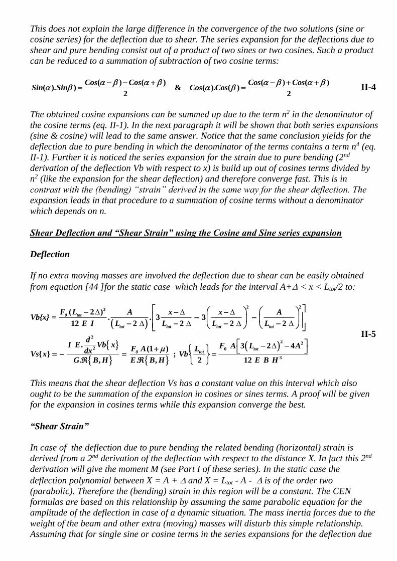
Calculation of Shear Deflection

-3,0E-06

-2,0E-06

-1,0E-06

0,0E+00

1,0E-06

2,0E-06

3,0E-06

4,0E-06

5,0E-06

6,0E-06

0 20 40 60 80 100 120 140 160 180 200

Number of terms

Sh

ea

r D

efl

ec

tio

n V

s

Un Series: Cos(x) Tn Series: Sin(x)

Figure 1 The development of the Shear Deflection using a Cosine (Un) and a Sine (Tn) series

3 When the load distribution is developed into a sine series, two solutions for the homogenous differential

equation are needed in order to fulfil both the requirements at x=0 and x=. Furthermore the derivate of

Tn{x} at x=0 equals {2n./L}.Tn{/2} 4 If = 0 the T2n-1 series alone do not satisfy the requirement for the shear force at x = 0. The T2n-1 series

will lead after derivation to a series of 1/(2n-1) terms. In order to satisfy the boundary restriction a solution

of the homogenous differential equation has to be added: - x/(2n-1). This solution will eliminate the shear

force after the derivation of the terms – x/(2n-1) at x = 0. However, the series 1/(2n-1) converges badly.

It is also possible to express Vs in Vb using equation 1a or equation 4. However equation 4

contains an unknown function in t and equation 1a is in fact similar to equation 10b because

the first term in equation 1a can be neglected compared to the second term. Therefore in the

Excel program only the final solution for Vt is obtained by developing Vs in cosine series.

Total Length Ltot equals the Effective Length Leff (=0)

In that case the basic series development Tn and Un are defined by the symbol Pn and Rn:

tot eff

n n n

eff eff

n n n

eff eff eff

If L = L ( =0) than:

x AT x P x Sin n Sin n P

L L

x A AU x R x Cos n Cos n R Cos n

L L L

Vb x V

2 1 2 1 2 1

2 2 2

{ } { } 2 1 . 2 1 ; {0} 0

{ } { } 2 . 2 1 ; {0} 2 1

{ }

n

n n

i

a n n n

n n

i i

g n n n n

n n n eff

x A e P x Vc x Vd x

AVs x V x H e R x H H H e Cos n

L

*2 1

* *2 2

,2 1 2 1 2 1

1 1

,2 2 2 0 0 2

1 1 1

{ } { } ; { } { } 0

{ } { } { } ; 2 1

[43]

7. SOLUTION FOR THE PSEUDO-STATIC CASE

In the pseudo-static case the inertia forces do not play a role. Therefore the ratio of Vs and

Vb can easily be determined from equation [4] by omitting the time dependent terms.

dI E Vb x

dxVs x In which E is the Stiffness of the beamG B H

2

2.

. ,

[44]

tot

0 tot

tot tot tot tot

tot0 tot

LFor (A ) x the bending deflection Vb is :

F L A x x AVb =

E I L L L L

dI E Vb x F A L AF A LdxVs Vb

G B H E B H

2 23

22 2

2 0

2

( 2 ). . 3 3

12 2 2 2 2

. 3 2 4(1 );

. , . , 2

E B H 312

[45]

tot

tot

tottot

LVs

HL F AVs A x

LG B H L AVb

2

0

2 2

2 4 1 ..{( ) }

2 2. { , } . 3 2 42

5 [46]

5 In ASTM standards A=L/3; Using = 2/3 the ratio will be: 2

123

54

2

2

L

H.μ.

LVb

LVs

0 tot

tot tot tot tot

For x A the bending deflection Vb is :

F L x A A xVb =

E I L L L L

2 23( 2 ) ( )

. . 3 312 2 2 2 2

[47]

dI E Vb x

FdxVs x A xG B H E B H

2

20

.(1 )

{ } .( ). ,

[48]

0 tot

For 0 x the bending deflection Vb is :

F L A A xVb =

E I

( 2 )

4

Vs x{0 } 0 [49]

In many textbooks and papers the value for is taken equal to 2/3. However, based on 1D,

2D and 3D finite element calculations with ABAQUS it was found that a value of 0,85 was

more appropriate. That’s to say the answers from 3D (and 1D) calculations are comparable

to the analytical solutions if a value of 0,85 was used. As expected the ratio depends on 3

parameters: Poisson ratio, the ratio H/L and the ratio A/L.

The value is obtained by comparing FEM calculations for the 1D case (bar elements) and

for the 2D case. In the 1D case it is possible to vary the stiffness modulus E and the shear

modulus G independently. In this way the deflections due to pure bending and shear can be

determined separately (by choosing an “infinite” value for G). Assuming that the 2D case

(and 3D case) will give correct answers the ratio Vs{Ltot/2}/Vb{Ltot/2} is determined. For

H/Ltot ratio of 25/450; 50/450 and 100/450 an value of 0,85 was established.

8. HOW TO INCORPERATE EXTRA MOVING MASSES.

The extra inertia forces are present in both differential equations:

i

mix mass mass

imix

mass mass

i t i t

S e I Vb x t B H Vb x t M Vt x t Q x tx t t

Se B H Vs x t M Vt x t Q x t

x t

Vb x t Vb x e Vs x t Vs x e Vt x t Vb x t Vs x t

4 2 2

4 2 2

2 2

2 2

{ , } { , } { , } { , }

{ , } { , } { , }2(1 )

{ , } { }. ; { , } { }. ; { , } { , } { , }

[50a,b]

In this report a correct solution procedure will be followed in contrast with a procedure

outlined in Part II “Overhanging Beam Ends and Extra Moving Masses” of these series. In

Part II the deflection due to shear was ignored and Vt{xmass,t} was taken equal to Vb{xmass,t}.

By multiple iteration (calculating Vb{xmass,t} and Vb{x,t} the ultimate deflection values were

established. This procedure was and is attractive because for the back calculation procedure

the extra moving masses could be incorporate in an easy way.

However, if the deflection due to shear is not ignored a different forward calculation has to

be performed. First of all the equations 50a,b are rewritten as:

i

mix mass mass mass

imix

mass mass mass

S e I Vb x t B H Vb x t Q x t M Vt x t xx t t

Se B H Vs x t Q x t M Vt x t x

x t

4 2 2

4 2 2

2 2

2 2

{ , } { , } { , } { , }. { }

{ , } { , } { , }. { }2(1 )

[51a,b]

In this way the forces due to an extra moving mass at a prescribed location are included in

the external (driven) force. In fact the same type of formulas as presented in chapter 6 can

be used if the force F is replaced by:mass mass

F F M Vt x2

0{ } according to equations [31]

to [33]. Because the influences of extra masses are for normal conditions small, a simple

iteration procedure can be performed:

1. The first step is the calculation of the bending and shear deflections at the desired

location x and the location(s) xmass where the extra moving masses are using the

equations for the system without extra moving masses.

2. Than the total deflection at xmass is calculated: Vt{ xmass} = Vb{ xmass } + Vs{ xmass }

3. The second step is the calculation of the deflections with extra moving masses in

which for the deflection Vt{ xmass } at the right hand side of equations [51a,b] the value

of the former step is taken.

4. Step 3 is repeated until the estimate value for Vt{ xmass } of the former step doesn’t

differ from the new estimated value for Vt{ xmass }

5. In the Excel program the iterations are not performed using e.g. Visual Basic.

Therefore the number of iterations is limited to nine steps which are in normally

situations enough.

ANNEX I “Development in Sine or Cosine Series”

In chapter 5 the load function Q was developed into infinite a series of sine or cosine

functions. With respect to the boundary conditions, the sine function series was adopted for

the deflection due to pure bending and the cosine function series was adopted for the

deflection due to shear. In this annex we will try the opposite.

Pure Bending

When a cosine function series is used the boundary condition for the second derivation is not

met. Therefore even in the case of no overhanging beam ends the solutions Vc{x} and Vd{x}

have to be added

ni i t

n n

nx x

Vb x t A e U x Vc x Vd x ex x

*0

2 2*

2 22,4,6,..0 0

{ , } . { } { } { } . 0

I-1

The other condition is that at the outer clamp the deflection should be zero.

ni t i i t

n n

n

Vb t Va Vc Vd e A e U Vc Vd e*

0 2 0*

2 2

1

{ , } { } { } { } . . { } { } { } . 0

I-2

Therefore we have two equations, which make it possible to calculate the coefficients Cn and

Dn of the deflections functions Vc{x} and Vd{x}.

Pure Shear

In case of the deflection due to shear it is also possible to solve the problem using sine

functions. However, the only acceptable solution of the homogenous differential equation for

the whole interval (0 x Ltot) is a single constant H0 times the time function. This is not

enough to satisfy both conditions: no shear at x=0 and no deflection at x=. However, an

acceptable solution will be possible if the interval 0 x Ltot is divided into 2 separate

intervals: 0 x Ltot /2 and Ltot /2 x Ltot. In the first interval we have the extra

solution H1.x + H0 and in the second interval the solution - H1.x + H0 + H1. Ltot.

xxLtotx Ltotx

n

tot tot tot

n

tot tot tot tot

x AT x Sin m Sin m Sin m

L L L

m x AT x Cos m Sin m Sin m

x L L L L0

0

22

{ } 2 1 . 2 1 2 1

2 1{ } 2 1 . 2 1 2 1

I-3

tot

n

x tot tot tot

tot n

x L tot tot tot

m AAt x T x Sin m Sin m

x L L L

m AAt x L T x Sin m Sin m

x L L L

0

2 10 : { } . 2 1 2 1

2 1: { } . 2 1 2 1

I-4

m

m tot tot tot

m

m tot tot tot

tot

tot

m ASin m Sin m

L L L

ASin m Sin m Sin m

L L L

L Sin mL

1

1

2 1. 2 1 2 1

. 2 1 . 2 1 2 1

. 2 1

m

m tot tot

ASin m Sin m

L L1

. 2 1 2 1

I-5

At x = Ltot /2 the deflection is continuous but the first derivate changes from sign.

ANNEX II “The series development for the deflection due to shear”

INTRODUCTION

In the “Handbook of Mathematical Functions” (M. Abramowitz & I.A. Segun; Dover

publications, Inc., New York) an overview is given of summable series consisting of either

sines or cosines.

e

n

n

n

Cos nLn Sin for

n

Cos nfor

n

Cos nfor

n

1

2 2

21

4 2 2 3 4

41

( )2 0 2

2

( )0 2

6 2 4

( )0 2

90 12 12 48

II-1

n

n

n

Sin nfor

n

Sin nfor

n

Sin nfor

n

1

2 2 3

31

4 2 3 4 5

41

( ) 10 2

2

( )0 2

6 4 12

( )0 2

90 36 48 240

II-2

The series e

n

Sin n tLn Sin dt

n21 0

( )2

2

{“Clausen’s Integral”} will converge for

0 but is not summable like the sine and cosine series given above. The Clausen’s

integral can only be expressed in another series representation:

nn

e

n

n n

Sin nLn B for

n n n n

12 ´ 1

221 1

1( )´ 0

2 ! 2 (2 1) 2

6 II-3

6 The coefficient B2n is not given in the “Handbook of Mathematical Functions” but can (probably) found in

“Tabulations of the function

12

)()(

n n

nSin ” by A. Ashour and A. Sabri (Math. Tables Aids Comp.,

1956)

This does not explain the large difference in the convergence of the two solutions (sine or

cosine series) for the deflection due to shear. The series expansion for the deflections due to

shear and pure bending consist out of a product of two sines or two cosines. Such a product

can be reduced to a summation of subtraction of two cosine terms:

Cos Cos Cos Cos

Sin Sin Cos Cos( ) ( ) ( ) ( )

( ). ) & ( ). ( )2 2

II-4

The obtained cosine expansions can be summed up due to the term n2 in the denominator of

the cosine terms (eq. II-1). In the next paragraph it will be shown that both series expansions

(sine & cosine) will lead to the same answer. Notice that the same conclusion yields for the

deflection due to pure bending in which the denominator of the terms contains a term n4 (eq.

II-1). Further it is noticed the series expansion for the strain due to pure bending (2nd

derivation of the deflection Vb with respect to x) is build up out of cosines terms divided by

n2 (like the expansion for the shear deflection) and therefore converge fast. This is in

contrast with the (bending) “strain” derived in the same way for the shear deflection. The

expansion leads in that procedure to a summation of cosine terms without a denominator

which depends on n.

Shear Deflection and “Shear Strain” using the Cosine and Sine series expansion

Deflection

If no extra moving masses are involved the deflection due to shear can be easily obtained

from equation [44 ]for the static case which leads for the interval A+ < x < Ltot/2 to:

0 tot

tot tot tot tot

tot0 tot

F L A x x AVb{x} =

E I L L L L

dI E Vb x F A L AF A LdxVs x Vb

G B H E B H E B H

2 23

22 2

2 0

3

( 2 ). . 3 3

12 2 2 2 2

. 3 2 4(1 ){ } ;

. , . , 2 12

II-5

This means that the shear deflection Vs has a constant value on this interval which also

ought to be the summation of the expansion in cosines or sines terms. A proof will be given

for the expansion in cosines terms while this expansion converge the best.

“Shear Strain”

In case of the deflection due to pure bending the related bending (horizontal) strain is

derived from a 2nd derivation of the deflection with respect to the distance X. In fact this 2nd

derivation will give the moment M (see Part I of these series). In the static case the

deflection polynomial between X = A + and X = Ltot - A - is of the order two

(parabolic). Therefore the (bending) strain in this region will be a constant. The CEN

formulas are based on this relationship by assuming the same parabolic equation for the

amplitude of the deflection in case of a dynamic situation. The mass inertia forces due to the

weight of the beam and other extra (moving) masses will disturb this simple relationship.

Assuming that for single sine or cosine terms in the series expansions for the deflection due

to pure bending the 2nd derivation of the deflection will lead to the correct strain value for

this deflection component, the bending strains are calculated in the Excel program. As

shown by calculations the differences in strain values with the static case are rather small

for low frequencies and low masses for the beam. Except for the case in which the chosen

location is equal or near to the position of the clamps (supports).

As can be obtained from the differential equation for the deflection Vs due to shear, a

(theoretical calculated) 2nd derivation with respect to x will lead to a zero value as expected,

even in the case of dynamic loading (without extra moving masses). A shear force does not

lead to a horizontal strain in the beam but will only deform the cross section of the beam.

This deduction is based on the formulas for the static and dynamic case in which no extra

moving masses are present. When an extra moving mass is present (e.g. the weight of the

plunger) the two principle differential equations are coupled by the mass inertia force at the

point where the mass is connected to the beam (often the two inner clamps or supports) and

the reaction forces at the two outer supports. Due to the extra term the phase lag for the

shear deflection will not have the same (but opposite) value as the phase lag of the complex

stiffness modulus for the beam. The difference is small but exists. Therefore the “shear

strain” “should” be calculated from the deflections which are based on an expansion in

sines or cosines terms. However, especially for locations at and near the clamps will lead to

lead to unrealistic strain values. Performing the “required” 2nd derivation will eliminate the

convergence of the expansion (the factor n2 will vanish in the denominator of the terms).

Only the appearance of an extra moving mass may give some convergence.

Shear Deflection Vs

Omitting the term for the phase lag and the time function, the solution in a series

development is given by equation II-6

tot

n n n n

n tot mix

F LVs x H U x U H

L S B H n

2

0

2 2 2 2 2 21

2 2(1 ){ } { } { } ; . .

(2 )

II-6

The series Un is given by equation II-7.

n

tot tot tot

x AU x Cos n Cos n Cos n

L L L2

{ } 2 . 2 2

II-7

Using equation II-4 equation II-7 can be rewritten as equation II-8

n

tot tot tot

tot tot tot tot

x AU x Cos n Cos n Cos n

L L L

x A x A x xCos n Cos n Cos n Cos n

L L L L

2{ } 2 . 2 2

2 2 2 2

2

II-8

n

tot tot tot

tot tot tot

AU Cos n Cos n Cos n

L L L

A ACos n Cos n Cos n

L L L

2{ } 2 . 2 2

2 22 2 1 2

2

II-9

If equals 0 equations II-8 and II-9 can be rewritten as:

tot tot tot

n n

tot

x A x A xCos n Cos n Cos n

L L L AU x U Cos n

L2 2

2 2 2 2

{ } ; {0} 2 12

II-10

Due to the term n2 in the denominator (see eq. II-6) these series can be summed up.

Applying equation II-1 leads for the interval A+ x Ltot/2 finally to the solution as given

by equation 45: tot

mix

L F AVs A x

S B H

0(1 )

{ }2

II-11

As mentioned before using the U2n{x} series will lead to a reasonable fast convergence for

the development of the series. This is due to the fact that the U2n{x} series already satisfy one

boundary restriction of the differential equation (shear force = 0 for x = 0).

Using the T2n-1{x} series is a different ‘story’. Specially when 0 the convergence is

‘gone’.

Horizontal “Shear Strain” Contribution(?)

The title of this paragraph is somehow misleading. As can be seen by the equations for the

shear deflection in chapter 7, the shear force will not contribute to the horizontal strain in

the beam in the case that there are no extra moving masses. But even when extra moving

masses are present, there ought to be no contribution. However, in that case the strain is

calculated by taking the second derivate of the deflection. And hence the convergence of the

series expansion is ‘lost’ while the term (2n-1)2 in the denominator of the terms is eliminated

by the derivation. Therefore it is better to calculate the strain in another way:

1. Define, in spite of the results of the 2nd derivate of the shear deflection, the

contribution of the shear force to the horizontal strain as zero.

2. Multiply the calculated or measured total deflection according to the following

formula: Vb x Vt xRatio x

* 1{ } { }.

{ } 1

3. For measuring the total deflection in the centre (Ltot/2) the Ratio is equal to:

tot

tot

tot tot

LVs x HL

Ratio x [Pseudo-static case]L L AVb x

2

2 2

{ } 4 1 .2{ }2 . 3 4{ }

2

And if the deflection is calculated or measured at the inner clamp by:

tot

HVs x ARatio x A [Pseudo-static case]

Vb x A L A

2

2 2

4 1 .{ }{ }

{ } . 3 4

4. In this way a good estimate for the deflection due to bending is obtained. By

multiplying this deflection with the following factor a good estimate is found for the

real horizontal strain value.

5.

tot

tot

tottot

LR x

A x L x A

HA Hx R x Vb x Vb x

x L x AL

3

*

2 2

* * *

3 2 2

12 2 1{ } .

3 2 3

3{ } . { }. { } . { }

3 2 34 2