Pump and Hydropower systems

Civil Engineering

Profª. Helena Margarida Machado da Silva Ramos

IST

iii

ACKNOWLEDGMENT

This document is a result of the support by Bentley’s WaterGEMS without which this investigation

would be much more difficult and for all the interest and availability to answer technical questions.

iv

v

ABSTRACT

The main objective of this work is, to analyse two different WSS regarding their operating rules and

efficiency. Two case studies were analysed. The first case study analysed was the Beliche system,

a WSS in Portugal. Several scenarios were compared regarding the energy production and

operation of the turbines in order to determine the best operating scheme, as well as an evaluation

concerning the viability of the installation of a third turbine in the system. The influence of the type

of valves used for the system control were also analysed in addition to an assessment of the effect

of a regulating tank and sensitivity analyses concerning the influence of its volume and the type of

control. The second case study was based on the Socorridos system, to minimize its operational

energy costs. Taking into account factors such as the average population demand curve, daily

energy tariffs, tank capacity, characteristic pump and turbine curves, the goal was to determine

what daily scheduling allowed the best economy possible. The scheduling optimization was

performed by computational modelling of the system with the aid of genetic algorithms.

At the end, the best scenario of turbine operation in the first case study is found corresponding to

the one with the turbine running at its maximum efficiency and only resorting to the second turbine if

necessary, with no restrictions concerning efficiencies and heads values. The installation of the

third turbine proved to be viable signifying a very important future improvement in the Beliche

system. This system can also be simulated with a regulating tank and improved in several ways

depending on which type of control and investment are pretended. If the system were controlled by

the water level the energy produced would increase a lot. In the case study of Socorridos the

results showed that an optimization of the system operation mode would produce much higher

profits. It was also concluded that the volume of the tanks has a big influence in the profits

generated with a linear increasing for the referenced operation mode of the system.

Keywords: Energy efficiency, Water supply systems, Hydropower, Pumped-storage, Operating

rules, Genetic algorithms.

vi

vii

RESUMO

O principal objetivo deste trabalho é, portanto, analisar dois sistemas de abastecimento de água

diferentes, relativamente às suas regras de funcionamento e eficiência energética. Foram

analisados dois casos de estudo: i) o primeiro caso de estudo analisado foi o sistema de Beliche.

Vários cenários foram comparados quanto à produção de energia e funcionamento das turbinas de

forma a determinar qual o melhor, bem como uma avaliação da viabilidade de instalação de uma

turbina extra no sistema. A influência do tipo de válvulas utilizadas e o efeito de um tanque de

regulação também foram analisados, assim como análises de sensibilidade relativas à influência

do seu volume e tipo de controlo; ii) o segundo caso de estudo foi baseado no sistema de

Socorridos. Tendo em conta fatores como a curva média de consumo da população, as tarifas

diárias de energia, a capacidade do tanque e as curvas características da bomba e turbina, o

objetivo foi determinar o horário de funcionamento que permitisse a melhor economia possível. A

otimização foi realizada por modelação computacional do sistema com recurso a algoritmos

genéticos.

No final, o melhor cenário de operação da turbina no primeiro de caso estudo é encontrado

correspondendo a uma turbina a funcionar na sua máxima eficiência e só recorrer à segunda

turbina, se necessário, sem restrições quanto à eficiência e quedas úteis. A instalação de uma

terceira turbina provou-se ser viável o que significa um melhoramento futuro muito importante no

sistema de Beliche. Este sistema também pode ser simulado com um tanque de regularização e

melhorado de várias maneiras, dependendo do tipo de controlo e de investimento pretendidos. Se

o sistema fosse controlado pelo nível de água a energia produzida iria aumentar muito. No caso de

estudo de Socorridos os resultados mostraram que a otimização do modo de operação do sistema

produziria lucros muito mais elevados. Concluiu-se também que o volume dos tanques tem uma

grande influência nos resultados gerados com um aumento linear para o modo de operação base

do sistema.

Palavras-chave: Eficiência energética, Sistema de abastecimento de água, Energia hidroelétrica,

Energia Hidroelétrica reversível, Regras de operação, Algoritmos genéticos.

viii

ix

AWARDS AND RECOGNITION

First place in the "Innovation in Hydraulic Engineering Design" category with the project

"Energy Production in Beliche WSS".

x

xi

CONTENTS

ACKNOWLEDGMENT.................................................................................................................. iii

ABSTRACT ................................................................................................................................... v

RESUMO ..................................................................................................................................... vii

AWARDS AND RECOGNITION ................................................................................................... ix

CONTENTS .................................................................................................................................. xi

LIST OF FIGURES ..................................................................................................................... xiii

LIST OF TABLES ....................................................................................................................... xvi

NOMENCLATURE......................................................................................................................xvii

ABBREVIATIONS .....................................................................................................................xviii

1. INTRODUCTION .................................................................................................................... 1

1.1. Scope ............................................................................................................................. 2

1.2. Objectives ....................................................................................................................... 4

1.3. Structure of the document ............................................................................................... 5

2. STATE-OF-THE-ART ............................................................................................................. 7

2.1. Common barriers to energy and water efficiency ............................................................. 8

2.2. Approaches to efficient water distribution ........................................................................ 9

2.3. Hydraulic turbomachinery ............................................................................................. 11

2.3.1. Hydraulic turbines ................................................................................................. 11

2.3.2. Rotodynamic pumps ............................................................................................. 13

2.3.3. Pump as turbine .................................................................................................... 15

2.3.4. Characteristic curves ............................................................................................. 17

2.3.5. Operating in parallel .............................................................................................. 19

2.3.6. Similarity laws ....................................................................................................... 20

2.4. Small hydropower economic analysis ............................................................................ 22

2.4.1. Economic analysis parameters .............................................................................. 22

2.4.2. Remuneration schemes ........................................................................................ 24

2.5. Pumped-storage power plants ...................................................................................... 24

2.6. Optimization ................................................................................................................. 26

xii

2.6.1. Methods of optimization ........................................................................................ 26

2.6.2. Genetic algorithms ................................................................................................ 27

3. CASE STUDY DESCRIPTION AND MODELLING ............................................................... 31

3.1. Case study A – Beliche system ..................................................................................... 32

3.1.1. System description ................................................................................................ 32

3.1.2. System modelling .................................................................................................. 35

3.1.3. System with regulating tank ................................................................................... 39

3.1.4. Summary of analyses performed ........................................................................... 40

3.2. Case Study B – Socorridos pumped-storage system ..................................................... 40

3.2.1. System description ................................................................................................ 40

3.2.2. System modelling ....................................................................................................... 45

3.2.3. Cost-effective optimization .......................................................................................... 46

4. ANALYSES AND RESULTS ................................................................................................ 52

4.1. Case study A – Beliche system ..................................................................................... 53

4.1.1. Analyses of different scenarios .............................................................................. 53

4.1.2. Installation of a third turbine .................................................................................. 60

4.1.3. Economic Analysis ................................................................................................ 61

4.1.4. System with regulating tank ................................................................................... 66

4.2. Case study B – Pumped-storage Socorridos system ..................................................... 68

4.2.1. Achievement of pump/turbine best schedule.......................................................... 68

4.2.2. Influence of the volume of the tanks ...................................................................... 73

5. CONCLUSIONS ................................................................................................................... 79

5.1. General Conclusions ............................................................................................................. 80

5.2. Further developments............................................................................................................ 81

6. REFERENCES ..................................................................................................................... 83

Consulted websites ...................................................................................................................... 88

A. APPENDICES ..................................................................................................................... A-1

xiii

LIST OF FIGURES

Figure 1.1| Electricity generated from renewable energy sources, EU-27, 2000-2010 (Eurostat) .... 2

Figure 1.2| Share of renewable energy in gross final energy consumption in EU-27 Member States

(APREN) ........................................................................................................................................ 3

Figure 1.3| Electricity generation in Portugal by technology, 2010 (REN) ....................................... 4

Figure 1.4| Structure of the document ............................................................................................ 6

Figure 2.1| Burst water main at high and low pressure (Barry, 2007) ............................................ 10

Figure 2.2| Three main types of water turbines: (A) Pelton wheel; (B) Francis turbine; (C) Kaplan

turbine (Darling, 2013) ................................................................................................................. 12

Figure 2.3| Overview of turbine runners and their operating regimes (Casey and Keck, 1996) ...... 13

Figure 2.4| Pump energy demands (Moreira, 2012) ..................................................................... 14

Figure 2.5| Types of pumps and relative flow direction and axis position (Engineering Science Data

Unit) ............................................................................................................................................. 15

Figure 2.6| Scheme of the four-quadrant performance of a pump/turbine (KSB, 2005) ................. 17

Figure 2.7| Performance curves in turbine and pump mode for different speeds (Chapallaz et al.,

1992) ........................................................................................................................................... 18

Figure 2.8| Operating point of a pump (Chapallaz et al., 1992) ..................................................... 19

Figure 2.9| Comparison between a single pump and two equal pumps in parallel (Chapallaz et al.,

1992) ........................................................................................................................................... 20

Figure 2.10| Pumped Storage Power Plant Operation Scheme (SCENE, Community Energy

Specialists) .................................................................................................................................. 25

Figure 2.11| Classification of a optimization problem (based on Sarker and Newton, 2008) .......... 27

Figure 2.12| Flowchart of the GA cycle (Lin, 2006) ....................................................................... 29

Figure 3.1| Operating scheme of the Eastbound system (Carriço et al., 2013).............................. 33

Figure 3.2| View of Beliche Dam tank and treatment plant at Algarve (Ramos et al., 2010) .......... 33

Figure 3.3| Scheme of the micro-hydro power plant ..................................................................... 34

Figure 3.4| View of the turbines inside the valve chamber ............................................................ 34

Figure 3.5| Turbine characteristic curves to 1500 rpm (50 Hz) (Livramento, 2013) ....................... 35

Figure 3.6| Scheme of the Beliche system under analysis ............................................................ 36

Figure 3.7| Characteristic curve of each turbine (adapted from Livramento, 2013)........................ 36

Figure 3.8| Daily water consumption factors considered in the analysis downstream of Beliche WTP

.................................................................................................................................................... 37

Figure 3.9| Mean daily flows in Beliche WTP ............................................................................... 37

Figure 3.10| Scheme of the Beliche system with a regulating tank ............................................... 39

Figure 3.11| Diagram of the Beliche system methodology ............................................................ 40

Figure 3.12| Multi-purposes scheme of Socorridos system under analyze .................................... 41

Figure 3.13| Socorridos storage tank: inlet tunnel (a) and centrifugal pump (b) ............................. 42

xiv

Figure 3.14| Socorridos pumping station: outside view (a); centrifugal pumps and control valves (b)

and (c) ......................................................................................................................................... 43

Figure 3.15| Socorridos pumping station: plant of the ground level (a), transversal view (b) and

longitudinal view (c)...................................................................................................................... 44

Figure 3.16| Characteristic curves of the turbine (a) and of the pump (b) ...................................... 44

Figure 3.17| St. Quitéria hydropower station: inside view of Pelton turbine (a) and (b) .................. 45

Figure 3.18| Water volume consumption Câmara de Lobos and inlet volume in Covão ................ 46

Figure 3.19| Electricity tariff used in the model both for sale and purchase of energy (Eletricidade

da Madeira).................................................................................................................................. 46

Figure 3.20| Optimization procedure ............................................................................................ 50

Figure 4.1| Comparison of the number of turbines theoretically operating based on the WTP flow

and the ones effectively producing energy based on its efficiency, in the month of May and for two

turbines installed .......................................................................................................................... 57

Figure 4.2| Flow variation for the month of August with a TCV installed ........................................ 58

Figure 4.3| Turbine flow during the day in function of the mean daily flows in the WTP in the system

whit a TCV installed ..................................................................................................................... 58

Figure 4.4| Flow variation for the month of August with a FCV and PRV installed ......................... 59

Figure 4.5| Turbine flow during the day in function of the mean daily flows in the WTP in the system

whit a FCV and PRV installed....................................................................................................... 59

Figure 4.6| Daily energy production due to the mean daily flow in the WTP .................................. 60

Figure 4.7| Comparison of the number of turbines theoretically operating based on the WTP flow

and the ones effectively producing energy based on the efficiency characteristic curve, in August

and for three turbines installed ..................................................................................................... 61

Figure 4.8| Curves for the hydropower equipment initial cost - pump operating as a turbine and

water turbine (adapted from Ramos e Ramos, 2010) .................................................................... 61

Figure 4.9| Comparison of the economic analysis of two and three turbines installed in the Beliche

hydropower plant for a period of 15 years and a discount rate of 4% for the remuneration scheme of

sale (a) and consumption in-situ (b). ............................................................................................. 64

Figure 4.10| Comparison of the NPV on the economic analysis of the installation of two or three

turbines with energy production during all year for the schemes of sale to national electric grid and

consumption in-situ ...................................................................................................................... 65

Figure 4.11| Sensitivity analysis of the installation of the third turbine to initial cost of the

hydropower equipment for the remuneration scheme of sale of the produced energy.................... 65

Figure 4.12| Variation of the turbine flow during the day in function of the demand at the WTP..... 66

Figure 4.13| Water level variation in a regulating tank with a maximum volume of 51050 m3 and an

admitted circular shape with a diameter of 50 m ........................................................................... 67

Figure 4.14| Energy produced per day on the micro-hydropower plant depending on the volume of

the tank of regularization for the month of June ............................................................................ 68

xv

Figure 4.15| Water level variation in Covão (a) and Socorridos (b) tanks for the base mode of

operation of the system and identification of the electricity tariff .................................................... 70

Figure 4.16| Pump and turbine operation time for the base mode of operation of the system........ 70

Figure 4.17| Water level variation in Covão (a) and Socorridos (b) tanks for the optimized mode of

operation of the system and identification of the electricity tariff .................................................... 72

Figure 4.18| Pump and turbine operation time for the optimized operation mode of the system .... 72

Figure 4.19| Water level variation in Covão (a) and Socorridos (b) tanks for the base operation

mode in function of the tanks volume (m3) .................................................................................... 74

Figure 4.20| Pump (a) and turbine (b) operation time for the base operation mode in function of the

tanks volume (m3) ........................................................................................................................ 75

Figure 4.21| Water level variation in Covão (a) and Socorridos (b) tanks for the optimized operation

mode of the system in function of the tanks volume (m3) .............................................................. 76

Figure 4.22| Pump (a) and turbine (b) operation time for the optimized mode of operation in

function of the tanks volume (m3) ................................................................................................. 77

Figure 4.23| Profits generated in the system for the two different modes of programming in function

of the volumes of Covão e Socorridos tank ................................................................................... 78

xvi

LIST OF TABLES

Table 3.1| Mean daily flows, in 2011, in the months of operation of the micro-hydro ..................... 38

Table 3.2| Summary of the different scenarios analysed concerning the turbine operation and

energy production ........................................................................................................................ 38

Table 3.3| System penstock characteristics .................................................................................. 45

Table 3.4| Characteristics of the tanks of the analysed system ..................................................... 45

Table 4.1| Mean of produced energy, in 2011, in the months of operation of the micro-hydro with 2

turbines installed considering them always performing at the same efficiency and for all head values

and efficiencies ............................................................................................................................ 53

Table 4.2| Mean of produced energy, in 2011, in the months of operation of the micro-hydro with 2

turbines installed considering one turbine at its maximum efficiency and the second only switched-

on if needed. Operation for all head and efficiency values ............................................................ 54

Table 4.3| Mean of produced energy, in 2011, in the months of operation of the micro-hydro with 2

turbines installed working if needed and neglecting the energy correspondent to small heads and

efficiency values lower than 35% .................................................................................................. 55

Table 4.4| Summary of the energy produced in the 148 days of operation of the micro-hydro ....... 55

Table 4.5| Results obtained in the WaterGEMS model concerning to a daily average demand of

62.05 l/s at WTP and necessary to calculate the energy produced................................................ 56

Table 4.6| Mean of produced energy, in 2011, in the months of operation and for arbitrated flow

values for the scenario of micro-hydro with 3 turbines installed working only if needed ................. 60

Table 4.7| Economic analysis of the existing scenario of two installed turbines in the micro-

hydropower plant for the two schemes of remuneration ................................................................ 62

Table 4.8| Economic analysis of the existing scenario of two installed turbines in the micro-

hydropower plant for the two schemes of remuneration and for arbitrated flow values................... 63

Table 4.9| Economic analysis of the installation of a third turbine in the micro-hydropower plant for

the two schemes of remuneration ................................................................................................. 63

Table 4.10| Economic analysis of the hypothesis of the installation of a third turbine in the micro-

hydropower plant for the two schemes of remuneration and for arbitrated flow values................... 64

Table 4.11| Mean of produced energy, in 2011, for the scenario of micro-hydro with an regulating

tank and controls depending on the tank level .............................................................................. 67

Table 4.12| Energy produced and consumed, and daily costs, benefits and profits ....................... 72

Table 4.13| Energy consumed and produced, daily costs, benefits and profits for different tank

volumes ....................................................................................................................................... 77

xvii

NOMENCLATURE

∆𝒕 Time interval (h);

𝑪𝑷 Energy cost of a pump (€);

𝒄𝑷,𝒉 Electricity tariff associated with the pump operation in each hour ((€/kWh);

𝒄𝑻,𝒉 Electricity tariff associated with the turbine operation in each hour ((€/kWh);

𝒅𝑵 Water level variation in Covão tank;

𝑬 Energy (kWh);

𝑯 Total head of hydraulic turbomachinery (m);

𝑯𝑷 Head of a pump (m);

𝑯𝑻 Net head of a turbine (m);

𝒏 Rotational speed of a turbine (rpm);

𝑵𝒔 Specific speed (rpm);

𝑷 Total power developed in hydraulic turbomachinery (W);

𝑷𝑷 Net power of a pump (W);

𝑷𝑻 Net power of a turbine (W);

𝑸 Flow rate (m3/s);

𝜸 Specific weight of the water (9800 N/m3);

𝜼 Overall efficiency of a hydraulic turbomachinery (-);

𝜼𝑷 Efficiency of the pump (-);

𝜼𝑻 Efficiency of the turbine (-).

xviii

ABBREVIATIONS

APREN Associação de Energias Renováveis;

BCR Benefit Cost Ratio ;

EA Evolutionary algorithm;

ENE National Energy Strategy;

EU European Union;

DGEG Direcção-Geral de Energia e Geologia;

GA Genetic Algorithm;

IRR Internal Rate of Return;

MMWSS Multi-Municipal Water Supply System;

NPV Net Present Value;

PAT Pump as Turbine;

PRV Pressure Reduction Valve;

PSPP Pumped-Storage Power Plants;

SRP Special Regime Production;

SQP Sequential Quadratic Programming;

TRUST Transitions to the Urban Water Services of Tomorrow

WTP Water Treatment Plant;

WSS Water Supply System.

1

1. INTRODUCTION

This chapter gives a brief introduction to the topic, allowing the reader to understand the context of

the study. It also presents the proposed goals and further a summary of the structure of the

document.

Content

1.1. Scope ............................................................................................................................. 2

1.2. Objectives ....................................................................................................................... 4

1.3. Structure of the document ............................................................................................... 5

1

2

1.1. Scope

The evolution of civilizations and the modern world is directly related to the energy needs. The

energy in its various forms is essential to all human activities and it is a critical factor for economic

and social development. Currently, the energy needs of the world are based mainly on the

exploitation of fossil fuels. The problem is that these needs have been increasing while the reserves

are depleted at a fast pace. It is estimated that by 2050 the energy demand could double or triple,

as the population increases and developing countries expand their business.

The energy and its more efficient use has, therefore, a huge importance in the operationalization of

sustainable development, being essential to develop strategies and long-term initiatives which allow

better utilization of energy resources. Although energy is associated with an increased comfort and

quality of life, its excessive consumption begins to be questioned since it can pose serious damage

to the environment. Indeed, it can have local and regional impact (such as air and water pollution or

modification of the ecosystem) and may have several impacts in terms of the global environment

such as emissions of Greenhouse Gases (GHG) derived from fossil fuels and the resulting climate

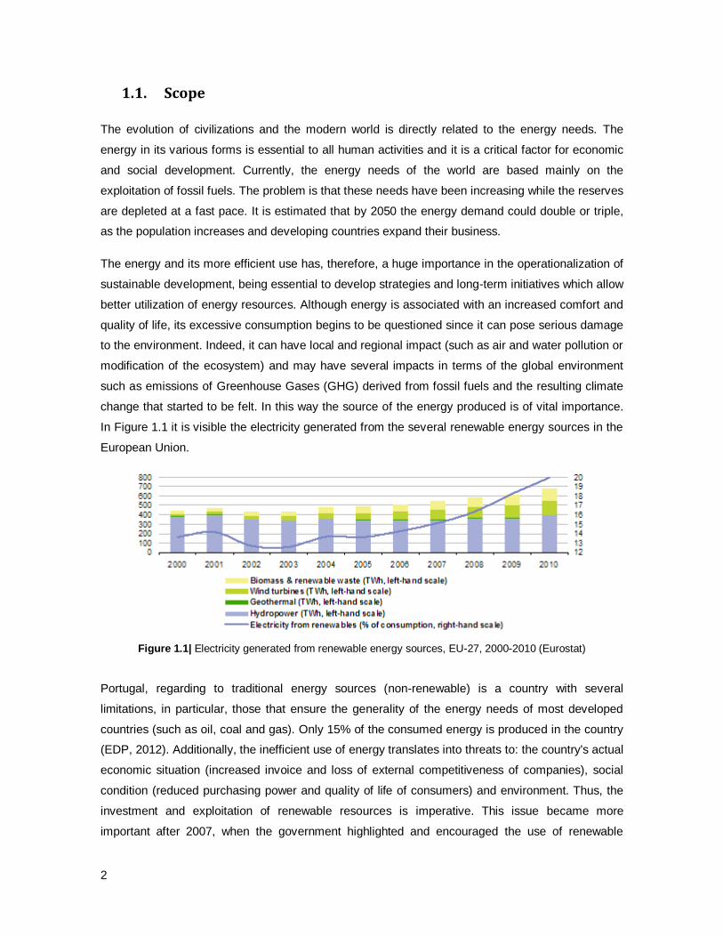
change that started to be felt. In this way the source of the energy produced is of vital importance.

In Figure 1.1 it is visible the electricity generated from the several renewable energy sources in the

European Union.

Figure 1.1| Electricity generated from renewable energy sources, EU-27, 2000-2010 (Eurostat)

Portugal, regarding to traditional energy sources (non-renewable) is a country with several

limitations, in particular, those that ensure the generality of the energy needs of most developed

countries (such as oil, coal and gas). Only 15% of the consumed energy is produced in the country

(EDP, 2012). Additionally, the inefficient use of energy translates into threats to: the country's actual

economic situation (increased invoice and loss of external competitiveness of companies), social

condition (reduced purchasing power and quality of life of consumers) and environment. Thus, the

investment and exploitation of renewable resources is imperative. This issue became more

important after 2007, when the government highlighted and encouraged the use of renewable

3

energies (APREN, 2011). Regarding the gross consumption of electricity in 2011 (Figure 1.2),

Portugal was recognized as the fifth country in the European Union with greater integration of

renewable energy, yet was considered the fifth country in the EU with greater energy dependence.

This dependence led to the development of ways to minimized it, resulting in a strong focus on

sector (DGEG, 2011).

Figure 1.2| Share of renewable energy in gross final energy consumption in EU-27 Member States (APREN, 2013)

Taking this situation into account, Portugal has set very ambitious goals in the energy sector.

According to the National Energy Strategy (ENE 2020), Portugal aims to reduce energy

dependence on the outside world from 83% in 2008 to 74% in 2020, which aims to incorporate 31%

of renewable energy consumption while it reduces by 20% the consumption. The investment and

development of renewable energy potential, which in Portugal is remarkable, especially for solar,

wind, hydro and biomass, is therefore one of the main goals. Figure 1.3 shows the electricity

generation in Portugal by the different sources and it is clear (and supported by Figure 1.1) that

water and energy are inextricably linked, and both are equally important for economic and

population growth (Lampe et al., 2009; Rio Carrillo and Frei, 2009).

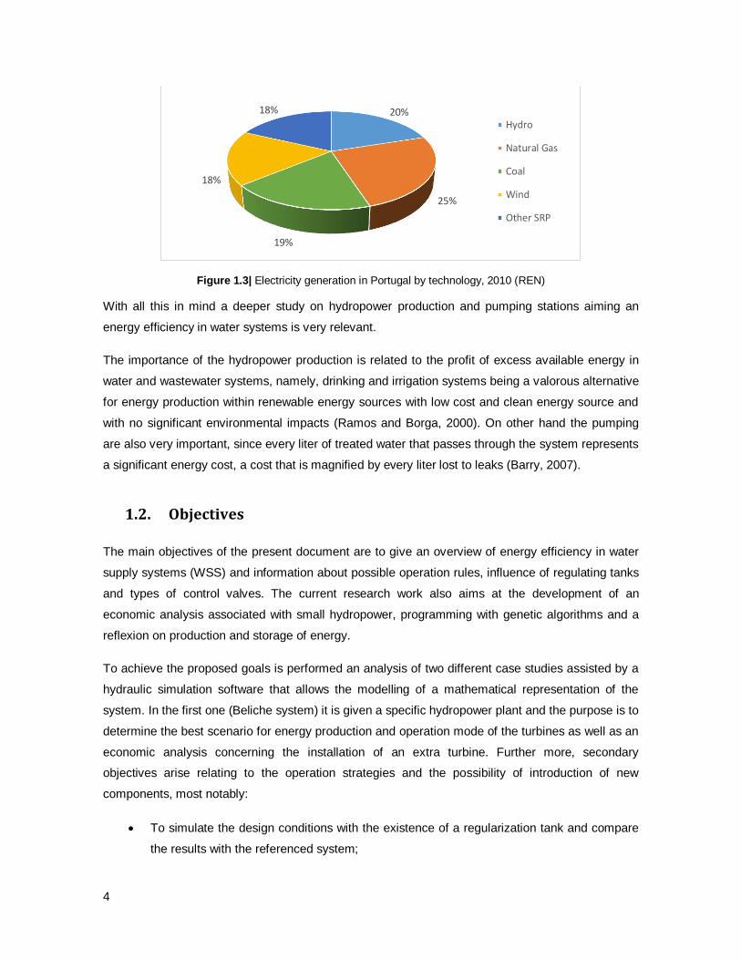
4

Figure 1.3| Electricity generation in Portugal by technology, 2010 (REN)

With all this in mind a deeper study on hydropower production and pumping stations aiming an

energy efficiency in water systems is very relevant.

The importance of the hydropower production is related to the profit of excess available energy in

water and wastewater systems, namely, drinking and irrigation systems being a valorous alternative

for energy production within renewable energy sources with low cost and clean energy source and

with no significant environmental impacts (Ramos and Borga, 2000). On other hand the pumping

are also very important, since every liter of treated water that passes through the system represents

a significant energy cost, a cost that is magnified by every liter lost to leaks (Barry, 2007).

1.2. Objectives

The main objectives of the present document are to give an overview of energy efficiency in water

supply systems (WSS) and information about possible operation rules, influence of regulating tanks

and types of control valves. The current research work also aims at the development of an

economic analysis associated with small hydropower, programming with genetic algorithms and a

reflexion on production and storage of energy.

To achieve the proposed goals is performed an analysis of two different case studies assisted by a

hydraulic simulation software that allows the modelling of a mathematical representation of the

system. In the first one (Beliche system) it is given a specific hydropower plant and the purpose is to

determine the best scenario for energy production and operation mode of the turbines as well as an

economic analysis concerning the installation of an extra turbine. Further more, secondary

objectives arise relating to the operation strategies and the possibility of introduction of new

components, most notably:

To simulate the design conditions with the existence of a regularization tank and compare

the results with the referenced system;

20%

25%

19%

18%

18%

Hydro

Natural Gas

Coal

Wind

Other SRP

5

To perform sensitivity analyses for key parameters/components of the models such as type

of valves, type of control and operation strategy.

The second case study is a pumped-storage hydropower system (Socorridos system) with water

consumption, inlet discharge and a defined operation schedule. The aim is to determine a new

operation schedule of the pump/turbines for one day with no hourly limitations, according to the

electricity tariff through an optimization model based on genetic algorithms and to access the

influence of the tank volumes in the profits generated.

1.3. Structure

The present document is divided into five chapters as displayed in Figure 1.4. In short, the first

chapter corresponds to the introduction, where a scope to address the subject is made and the

main objectives are presented. In chapter 2 an overview of energy efficiency in water supply

systems and the theoretical fundaments of hydraulic turbomachinery are presented. Also in this

chapter, reference is made to the particularities of conducting an economic analysis of hydropower

stations as well as the theory of pumped-storage hydropower plant systems and the basics of an

optimization through genetic algorithms. The methodology and applications are presented in

Chapter 3, describing the two case studies and the respective characteristics. Chapter 4 presents a

discussion of the computational results for the conditions of both studies as well as an economic

analysis concerning the viability of placing a third turbine in the Beliche system. The last chapter

(chapter 5) presents the general conclusions of this thesis and some recommendations for future

works.

6

Figure 1.4| Structure of the document

7

2. STATE-OF-THE-ART

This chapter provides an overview of energy efficiency in water supply systems networks and

measures based on rules, flow and devices behavior that can be taken to improve it. The theoretical

and mathematical bases concerning the operation of hydraulic turbomachinery (pumps and

turbines) are presented as well as the particularities of conducting a viability analysis associated to

a small hydropower scheme. Following, it is presented a brief description of pumped-storage power

plant systems and the theory and a survey of works existing on genetic algorithms.

Content

2.1. Common barriers to energy and water efficiency ............................................................. 8

2.2. Approaches to efficient water distribution ........................................................................ 9

2.3. Hydraulic turbomachinery ............................................................................................. 11

2.4. Small hydropower economic analysis ............................................................................ 22

2.5. Pumped-storage power plants ...................................................................................... 24

2.6. Optimization ................................................................................................................. 26

2

8

2.1. Common barriers to energy and water efficiency

The water-energy nexus is based on the reality that every liter of water that passes through a

system represents a significant energy value. This value can be translated into costs when it is

referred to treating water for human consumption and moving it to the consumer or in profit when it

is referred to energy production. In any case, most of the times the system is not working with its

best efficiency due to:

Inefficient pump/hydropower stations;

Poor design or installation;

Lack of maintenance or poor management;

Old pipes with high head loss;

Excessive supply pressure and head losses;

Leakage in the system;

Inefficient use of water;

Inefficient operation strategies.

This kind of problems that are crucial to solve in Water Supply Systems (WSS) exist because,

according with Barry (2007), there are serious obstacles to the widespread adoption of more

efficient practices and technologies, like:

Lack of awareness: People will not make changes towards efficiency unless they are

aware of the cost-benefit arguments for doing so;

Aversion to risk: Deviating from the usual routine is associated with risk, real or perceived,

such as added burden on staff or financial risk. Fear of change has a rational basis and

breaking through it requires that the fears be addressed and that the benefits of change

clearly outweigh risks;

Financing efficiency: For those that do require capital outlays, performance contracting

approaches pay for project costs from the cost savings on water and energy. Those

contemplating efficiency improvements often lack an understanding of performance

contracting mechanisms, especially the awareness that they can be applied to the water

sector. In some countries, financing issues are compounded by an insufficient supply of

service providers capable of performance contracting, or the suppliers exist but the industry

is so recent that confidence in them is lacking. This lack of confidence usually translates

into an inability of these firms to provide the project financing, since their unproven

creditworthiness either denies them access to loans altogether, or the terms are poor.

9

When the average water losses are estimated in 30%, it means that, at least, the same portion of

energy is lost. It is very important to overcome those obstacles and embrace new measures to

reach the best efficiency in all WSSs.

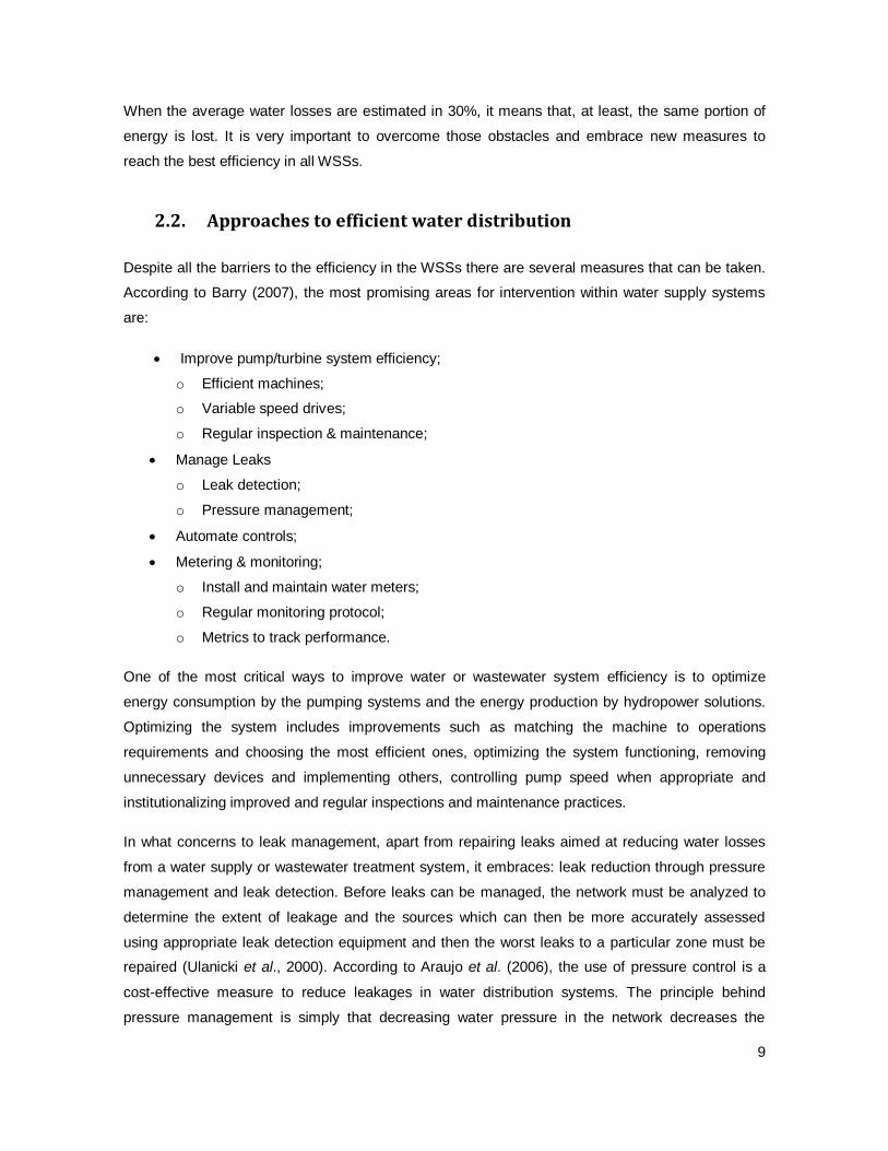
2.2. Approaches to efficient water distribution

Despite all the barriers to the efficiency in the WSSs there are several measures that can be taken.

According to Barry (2007), the most promising areas for intervention within water supply systems

are:

Improve pump/turbine system efficiency;

o Efficient machines;

o Variable speed drives;

o Regular inspection & maintenance;

Manage Leaks

o Leak detection;

o Pressure management;

Automate controls;

Metering & monitoring;

o Install and maintain water meters;

o Regular monitoring protocol;

o Metrics to track performance.

One of the most critical ways to improve water or wastewater system efficiency is to optimize

energy consumption by the pumping systems and the energy production by hydropower solutions.

Optimizing the system includes improvements such as matching the machine to operations

requirements and choosing the most efficient ones, optimizing the system functioning, removing

unnecessary devices and implementing others, controlling pump speed when appropriate and

institutionalizing improved and regular inspections and maintenance practices.

In what concerns to leak management, apart from repairing leaks aimed at reducing water losses

from a water supply or wastewater treatment system, it embraces: leak reduction through pressure

management and leak detection. Before leaks can be managed, the network must be analyzed to

determine the extent of leakage and the sources which can then be more accurately assessed

using appropriate leak detection equipment and then the worst leaks to a particular zone must be

repaired (Ulanicki et al., 2000). According to Araujo et al. (2006), the use of pressure control is a

cost-effective measure to reduce leakages in water distribution systems. The principle behind

pressure management is simply that decreasing water pressure in the network decreases the

10

volume of water escaping through any existing hole or leak in the pipe, as demonstrated by Figure

2.1. Also, in addition to reducing the existing leaks and preventing the emergence of new

leaks, pressure management reduces the incidence of pipeline ruptures, avoiding the

associated repair costs as well as the disruption of traffic on public roads and the supply of water to

the customers. According to Covas and Ramos (1999 and 2010), leakages can be modeled as

energy leaving the control volume, which is analogous to the hydraulic power supplied to

consumers in the form of the network pressure. Therefore, the use of devices, such as pressure-

reducing valves (PRVs) in particular, to increase the head losses in the network is the most

frequently used technology for pressure management and leakage reduction.

Figure 2.1| Burst water main at high and low pressure (Barry, 2007)

Automation in a water supply or wastewater treatment system monitors various system components

for optimal system performance and efficiency. Automation varies in complexity but it always has at

its core sensors that measure system parameters such as pressure, water level and flow rates. The

most basic and inexpensive form of automation consists of stand-alone devices that act on the

information from the sensor to perform simple actions only at the site where they are placed, such

as an automatic shut-off valve responding to water level indicator.

In water systems around the world only about 35% of consumption and 50% of supply is metered

making it difficult to improve a system performance. To achieve a more efficient system, the

establishment of a system to regularly monitor the various components and locations within the

water or wastewater system is crucial. Therefore it is important to create a system for water

metering and monitoring (if there is none) or expand and upgrade the existing system, developing

baselines and metrics for regular monitoring and creating targets and gauge success towards

achieving them against baselines and benchmarks.

In addition to the promising areas for intervention proposed by Barry (2007), and according to

Tsutiya (2005), the reduction in the rate of water losses and water conservation have significant

11

influence on the cost of electricity. This happens because with the reduction of the volume of water

to be wasted there will be a decrease in energy consumption. Identifying points of excessive energy

use after a diagnosis system in operation, it is possible to reduce the cost of electricity in a WSS.

After the deployments of energy efficiency measures in the system it is necessary to perform some

administrative actions aiming at the optimization of electromechanical and hydraulic optimization,

taking into account the operational aspects of the system.

2.3. Hydraulic turbomachinery

2.3.1. Hydraulic turbines

Hydraulic turbomachinery are machines that promote the exchange of mechanical energy between

the water and the rotor. To the movement of the fluid are associated forces that are developed in

the fluid mass and the engine blades (or wheel) in consequence of its rotation. These devices

always involves an energy transfer between a flowing fluid and a rotor and can be classified as an

hydraulic turbine if the transfer of energy is from the fluid to the rotor or as a pump, if the flow of

energy is from rotor to fluid (Logan, 1993).

The turbines are powered from a hydraulic head available, transforming it into mechanical energy

and then into electricity through a generator. The classification of turbines depends on how the flow

hits on the rotor, which allows to classify turbines in action and reaction turbines. When the rotor

blades are driven by water at atmospheric pressure it is classified as impulsive or action turbines.

Pelton turbines are the action turbines more used (Figure 2.2 (a)). In reaction turbines it is the force

of flow pressure that drives the rotor. The reaction turbine is further classified into radial, axial or

mixed flow turbines, depending on the direction of the main fluid path relative to the rotor (Quintela,

2009).

In turbines the flow direction relatively to the rotor has always a significant axial component

otherwise the flow would converge to the periphery of the rotor inducing a speed increase that

would lead to a reduction in the efficiency. The turbines in which the axial component of the flow is

less pronounced the runoff occurs mainly in the plane of rotation. These turbines are designed as

radial flow turbines, being Francis turbines one type of them (Figure 2.2 (b)).

On the other hand there are axial flow turbines when the main direction of the flow is parallel to the

axis of rotation at inlet and outlet of the runner and the fluid passes through the runner in surfaces

with almost constant radius. In this case we have propeller (fixed blades) or Kaplan (variable pitch

blades) turbines (Figure 2.2 (c)).

12

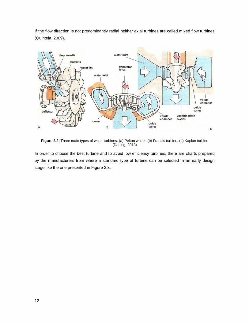
If the flow direction is not predominantly radial neither axial turbines are called mixed flow turbines

(Quintela, 2009).

Figure 2.2| Three main types of water turbines: (a) Pelton wheel; (b) Francis turbine; (c) Kaplan turbine (Darling, 2013)

In order to choose the best turbine and to avoid low efficiency turbines, there are charts prepared

by the manufacturers from where a standard type of turbine can be selected in an early design

stage like the one presented in Figure 2.3.

13

Figure 2.3| Overview of turbine runners and their operating regimes (Casey and Keck, 1996)

The net flow power of a turbine,𝑃𝑇, is given by equation (2.1) and is measured in Watts (W). It

depends on its efficiency, 𝜂𝑇, the specific weight of the water (9800 N/m3), 𝛾 , the turbine discharge

𝑄 (m3/s) and the net head (m), 𝐻𝑇.

𝑃𝑇 = 𝜂𝑇. 𝛾. 𝑄. 𝐻𝑇 (2.1)

The corresponding energy, E (kWh), over a time interval, T (h), of the hydropower plant will be

respectively:

𝐸 = ∫ P

𝑇

0

𝑑𝑡 (2.2)

This energy produced by the turbines is considered a clean energy as the turbine causes

essentially no change to the water.

2.3.2. Rotodynamic pumps

There is a need to move liquids, especially water, from one place, or from one level, to another. The

pumps are the turbomachines which allow this task. The rotodynamic pumps move the water by

dynamic action resulting from transfer angular momentum to the fluid using the mechanical energy

14

they receive from the electric motors that are coupled. They receive power from an external source

(engine) and give part of it to the fluid in the form of pressure, kinetic energy or both, i.e., they

increase the pressure and/or the velocity of the liquid (Torreira, 2002).

This type of pump has an operating principle the transmission to the liquid mass an acceleration so

that it acquires kinetic energy from the conversion of mechanical energy to potential energy

(pressure energy) by the movement of the rotor inserted in the pump body (Macintyre, 1980). Thus,

the movement of fluid occurs through the action of forces which are developed by the rotation of

shaft coupled to the wheel (rotor impeller) with blades, which receives the fluid through its center

and expellees it by the periphery, under the action of the centrifugal force. The movement induced

by the rotor produces kinetic energy, which is partly converted to pressure inside the pump, allowing

in that way the liquid to reach higher or distant positions through the compression pipe. A scheme

representing the energy demands of the pump are shown in Figure 2.4.

Figure 2.4| Pump energy demands (Moreira, 2012)

According to the different shapes and types of the rotor and the flow direction, it is possible to

distinguish the pumps, which can be classified as well as the reaction turbines as radial, axial or

mixed-flow pumps.

The radial or centrifugal pumps (Figure 2.5 (a)), have this name because of the flow path within the

rotor, which is made according to a radial plane (normal to the axis), from the center to the

periphery of the rotor. Mixed-flow pumps (Figure 2.5 (b)), have an impeller type whose flow is

diagonal to the axis, the fluid experiences both radial acceleration and lift and exits the impeller

somewhere between 0 and 90 degrees from the axial direction. Therefore it function as a

compromise between radial and axial-flow pumps. As a consequence mixed-flow pumps operate at

higher pressures than axial-flow pumps while delivering higher discharges than radial-flow pumps.

The exit angle of the flow dictates the pressure head-discharge characteristic in relation to radial

and mixed-flow.

On other hand the axial pumps (Figure 2.5 (c)) have flow trajectories in the direction of the axis of

the pump, being used for large flows and low manometric heights. The axial pumps do not use

15

centrifugal force, but the lift force (inertia). To increase this force, the rotor has an aerodynamic

profile with aspect of propeller.

(a) Radial pump (b) Mixed-flow pump (c) Axial pump

Figure 2.5| Types of pumps and relative flow direction and axis position (Engineering Science Data Unit,

2014)

The hydraulic power of a pump (Pp) measured in watts (W) depends on the mass flow rate, the

liquid density and the manometric head, as present in equation (2.3),

𝑃𝑃 =𝑄. 𝛾. 𝐻𝑝

𝜂𝑃 (2.3)

being Q the discharge (m3/s), 𝐻𝑝 the total pump head (m) and 𝜂𝑃 the efficiency of the pump.

The cost of pumping is mainly associated with the power consumed by the motors that drive the

pumps and which depends on the efficiency of the motor itself and the efficiency of the pump at a

given discharge rate.

The energy cost represent about 50% of the global cost of a pump and can be divided in fix and

variable costs. The variable costs depend on the unitary energy price during a specific period

determined by the electric company’s energy tariff and the amount of time during which the pump

operates.

𝐶𝑝 = 𝑃𝑃. 𝐶𝑝,ℎ . ∆𝑡 (2.4)

where 𝐶𝑝 is the energy cost of the pump (€), 𝑃𝑃 is the electric power of the pump (kW), 𝐶𝑝,ℎ is the

unitary cost of energy (€/kWh) and ∆𝑡 is the time interval of pump operation (h).

2.3.3. Pump as turbine The pump is presented as an economic advantage for being a machine on the market at acceptable

prices (Naldi et al. 2009). When a pump induces certain energy to the flow, it is necessary that this

16

quantity promotes the pumping of fluid, which in many cases cannot occur leading to a reverse

rotation of the wheel and therefore changing the flow direction from the local of discharge to the

draft tube. This situation is identified as a pump operating as a turbine (PAT).

A PAT operates as a reaction turbine with reverse flow, from the outlet to inlet. Since it has no flow

regulation (guide vane) it can only operate under approximate constant head and discharge.

Usually, this type of reversible turbines is used in pumped storage plant. One of the disadvantages

of these reversible turbomachinery is that it has lower efficiency than the simple turbines (Massey,

2006). On the other hand, the advantages of the system PAT among others, include: mechanics

implicitness, robustness, economically attractive (price and maintenance) and high hydraulic

performance.

Actually, the pumps operating as turbines is not a new idea, but a vast lack of knowledge in the

physical development of the fluid inside these devices has so far been an extremely delicate task

(Carravetta et al., 2012 and 2013). From this situation, the use of computational resources for the

understanding of the physical environment of a PAT allows not only to examine but also to bring

favorable solutions accompanied by experimental tests.

An application of a PAT in water supply or distribution systems was investigated by Naldi et al.

(2009) where three different perspectives of energy production are analyzed: a turbine, a PAT with

and without flow control and a PAT with flow control. In fact, when compared to conventional

turbines, pumps operating as turbines do not have a guide vane, so it is not possible to adjust the

machine flow to maintain optimal conditions for efficiency. Then, the main interest is the

assessment of the best efficiency to net head and flow values in the turbine mode and the

relationship between the values that lead to the best efficiencies in the pump mode.

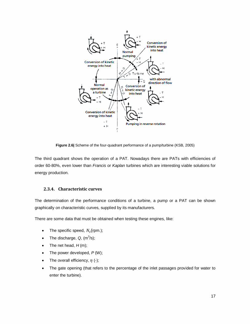
In Figure 2.6 it is possible to observe the four quadrants of performance of a pump and turbine.

17

Figure 2.6| Scheme of the four-quadrant performance of a pump/turbine (KSB, 2005)

The third quadrant shows the operation of a PAT. Nowadays there are PATs with efficiencies of

order 60-80%, even lower than Francis or Kaplan turbines which are interesting viable solutions for

energy production.

2.3.4. Characteristic curves

The determination of the performance conditions of a turbine, a pump or a PAT can be shown

graphically on characteristic curves, supplied by its manufacturers.

There are some data that must be obtained when testing these engines, like:

The specific speed, 𝑁𝑠(rpm.);

The discharge, Q, (m3/s);

The net head, H (m);

The power developed, P (W);

The overall efficiency, 𝜂 (-);

The gate opening (that refers to the percentage of the inlet passages provided for water to

enter the turbine).

18

The characteristic curves obtained can be constant head, speed and efficiency curves. A given

machine works with flows and net heads ranging within certain values. However, usually, the

specific speed remains constant because of the need to conserve practically invariable the

frequency of the power grid. Figure 2.7 shows typical pump and turbine curves for different

rotational speeds.

Figure 2.7| Performance curves in turbine and pump mode for different speeds (Chapallaz et al., 1992)

Each pair of values of flow and net head in which a given turbine operates at steady regime

(constant n), corresponds to a certain value of efficiency. The higher efficiency, to the possible

performance points with n constant, is called optimal efficiency that corresponds to the optimal

operation (Quintela, 2009).

The operating point corresponds to the intersection, at the plan (H, Q), of the characteristic curve of

the machine, H = H (Q), with the rotational speed number of the engine, n, with the curve that

expresses, as a function of flow rate, the total net head required for installation. The installation or

system curve is a graphical representation of the relation between discharge and head loss in a

system of pipes. It is completely independent of the pump characteristics and its basic shape is a

parable which stars at zero flow and zero head if there is no static lift, otherwise it would be

vertically offset from the zero head value. Figure 2.8 shows the operating point as a result of

interception of the pump and system curves.

In a pumping system consisting of a pump, a pipe and a tank, it is clear that the point where the

system and the pump curves cross change over time. This is due to the fact that some

characteristics of the system are altered, such as pipe roughness, pump wear, pump speed

changes or variations in the water level of the upstream tank. Those nonlinear phenomena are

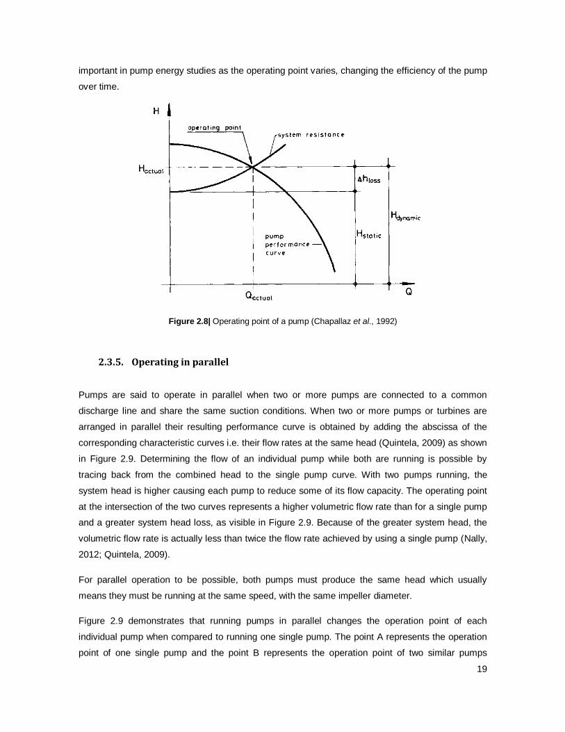
19

important in pump energy studies as the operating point varies, changing the efficiency of the pump

over time.

Figure 2.8| Operating point of a pump (Chapallaz et al., 1992)

2.3.5. Operating in parallel

Pumps are said to operate in parallel when two or more pumps are connected to a common

discharge line and share the same suction conditions. When two or more pumps or turbines are

arranged in parallel their resulting performance curve is obtained by adding the abscissa of the

corresponding characteristic curves i.e. their flow rates at the same head (Quintela, 2009) as shown

in Figure 2.9. Determining the flow of an individual pump while both are running is possible by

tracing back from the combined head to the single pump curve. With two pumps running, the

system head is higher causing each pump to reduce some of its flow capacity. The operating point

at the intersection of the two curves represents a higher volumetric flow rate than for a single pump

and a greater system head loss, as visible in Figure 2.9. Because of the greater system head, the

volumetric flow rate is actually less than twice the flow rate achieved by using a single pump (Nally,

2012; Quintela, 2009).

For parallel operation to be possible, both pumps must produce the same head which usually

means they must be running at the same speed, with the same impeller diameter.

Figure 2.9 demonstrates that running pumps in parallel changes the operation point of each

individual pump when compared to running one single pump. The point A represents the operation

point of one single pump and the point B represents the operation point of two similar pumps

20

running in parallel. When traced back, the operation point of a single pump operating in parallel,

which is the point B1, drifts upward due to a higher system head. If one pump was designed to

operate independently near its best efficiency point (point A), two similar pumps operating at the

same time will have a lower efficiency.

Figure 2.9| Comparison between a single pump and two equal pumps in parallel (Chapallaz et al., 1992)

If the pumps are of different sizes, the larger pump can throttle the smaller pump causing it to run

too far off of its best efficiency point. This can cause shaft deflection and possible premature

bearing and seal failure as the pumps will operate less efficiently (Nally, 2012).

2.3.6. Similarity laws

The vast majority of hydraulic structures is designed based on tests with reduced scale models.

According to Ramos (1999) the theory of similarity in turbomachinery is used in different types of

application and is extremely important in the areas of research based on experimental models

reduced.

The physical similarity is a general term that encompasses many different types of similarity,

namely: geometric similarity, kinetics similarity and dynamic similarity. Two systems are said to be

physically similar with respect to certain physical quantities, when the relationship between values

and corresponding counterparts of these quantities is constant in the whole of the two systems, the

prototype and its reduced model. For the geometric similarity, the dimensions of the turbomachine

cannot be reduced to a very small scale prototype otherwise it could be subject to scale effects. The

kinematic similarity implies equivalent velocity triangles at inlet and outlet of the runner and

21

in the case of dynamic similarity the polygon of forces should be similar both in prototype and in the

model (Ramos, 1999).

According to Ramos (1999, 2003) the similarity of Reynolds is not valid due to the fact that the

value of the Reynolds number is lower in the model or in the laboratory set-up than in the prototype.

On the contrary, the use of the similarity of Froude ensures the ratio between the inertial forces and

gravitational forces both in the prototype model as well as the similarity of the pressure gradient for

a given average speed. Establishing these conditions allows a scientific approach to select the

turbine that best fits the design conditions.

According to Quintela (2009), the similarity of hydraulic turboachinery is a particular case of

dynamic similarity. In order to obtain relationships between variables characteristics of hydraulic

turbines, from the laws of similarity, it can be considered that turbomachinery geometrically similar

work in similar conditions provided they have the same efficiency.

Thus, to one machine working under similarity conditions are observed the following relationships:

𝑛

𝑛′=

𝑄

𝑄′= (

𝐻

𝐻′)

12

= (𝑃

𝑃′)

13 (2.5)

Where n represents the rotational speed (rpm), Q is the discharge (m3/s), H is the net head (m) and

P is the power developed (W).

To establish the condition of equal efficiency of two geometrically similar turbines there are used,

according to Ramos (1995) and Quintela (2009), the expressions providing the turbine speed, head

and power, both in model and prototype:

𝑛

𝑛′= (

𝑃

𝑃′)

12

(𝐻

𝐻′)

54 (2.6)

Which results, according to the affinity laws, in equation (2.7).

𝑁𝑠 = 𝑛 𝑃

12

𝐻54

(2.7)

where 𝑁𝑠 is the specific speed of a similar turbine with unit head and unit output power during

similar operating conditions (rpm). Thus, the value of 𝑁𝑠 is considered as constant for similar

turbines, under the same conditions.

22

In what concerns to pumps, the specific speed of a given pump is the rotational speed of a pump

geometrically similar to the first one that, with equal efficiency, propels a unitary flow at a unitary

total head. This specific speed is given by the equation (2.8).

𝑁𝑠 = 𝑛 𝑄

12

𝐻34

(2.8)

2.4. Small hydropower economic analysis

2.4.1. Economic analysis parameters

The production of small-scale hydropower (micro-hydro) has been developed as a renewable

energy solution particularly in water supply systems (WSS). This solution has the advantages of

using components that already exist (tanks, pipes, valves) not being necessary large civil works and

the guaranteed of a continuous daily flow along each day (Vieira and Ramos, 2008).

The viability of hydropower production in small plants can be seen from the standpoint of interest

both for the national economy and for the operator, particularly, to the owner of the hydro plant

concerned. It should be noted that the contribution of small hydropower plants is usually negligible

in view of the productivity of the country. However, what matters is that the potential for substitution

with advantage of production in numerous and potential small hydropower is exploited to its limit.

This is all the more relevant as Portugal is a country with a lack of solid, liquid and even nuclear

fuels making its economy vulnerable both in relation to security of supply, as in matters of energy

prices. This type of electricity production is defined as micro, since it consists of a small-scale

activity of decentralized production, using for such renewable resources and delivering for

remuneration electricity to the public network, provided that there is actual consumption at the

installation site.

The final decision on whether or not an hydraulic project like a hydropower scheme should be

constructed, or the selection among alternative design solutions for the same, generally depends

on the comparison of the expected costs and benefits for the useful life of the project, by

means of economic analysis criteria.

The monetary base flows necessary to this type of economic analysis refer to the investment costs,

the operating costs (operation, maintenance, and parts of the reserve), the replacement and

revenue. There is always an investment period during which income may be nil or lower than costs,

followed by a revenue period when incomes exceed costs and the investment is earning its return.

A year is the standard unit and it is usually used as an account period in all financial analysis. The

23

respective estimates are based on market prices referred to a given year, the one during which the

studies were performed. The evolution of the inflation during the project lifetime and its effect on

each component of the previous cost estimates is practically impossible to establish. To overcome

the problem of future evolution of the inflation a common and simple economic approach based on

a constant market prices system referred to the year in study is generally applied in the comparison

of costs and benefits either of a project or of alternative design solutions for the same. This

approach assumes that it is not necessary to account for the inflation, as it will have the same effect

in any monetary flux. The future costs and benefits are, then, evaluated at present market prices.

(Portela, 2010).

In the course of an economic analysis there are some concepts that is necessary to understand:

Discount rate (r): The present value of a future unitary monetary flux will be lesser through

the years, which will generate different “appetencies” to transfer money from the present to

the future and vice-verse. Theses “appetencies” can be expressed in terms of different

discount rates. The values of these rates depend, among other factors, on the state of the

economy, on the risk that involves the investment, the capital availability and on the

expected future rate of inflation. One monetary unit of today will be changed in year n by

(1+r)n monetary units and one monetary unit of year n will be change today by 1/(1+r)

n

units.

Net Present Value (NPV) is the net sum of total discounted benefits and total discounted

costs in period of time. This shows the excess (or shortfall) of benefits over costs in

monetary terms.

Benefit Cost Ratio (BCR) is the ratio of total discounted benefits to total discounted costs.

A BCR greater than one should indicate a viable project.

Internal Rate of Return (IRR) is defined as the discount rate at which the NPV is zero. It is

the rate at which the project’s benefits are equal to the costs, and reflects the rate at which

the project investment is just recovered. Since the IRR is a measure of efficiency it is the

most widely used of the measures. It also has the advantage of not requiring a definite

discount rate specified in advance. Usually donors and governments have a target rate or

cut-off rate and projects with an IRR above the target rate are considered viable.

When considering a number of projects, the funding authorities may want to consider all three

measures, but NPV and IRR are the most commonly used. Analysis of NPVs can relate the scale of

project benefits (increase in national income) to the scale of the initial investment in ways which the

relative measures of the BCR and IRR cannot. On the other hand the IRR indicates the relative

efficiency of projects which the NPV does not. In the case of mutually exclusive projects, where only

one can be chosen because of competition for sites or other resources, the NPV would generally be

24

used rather than the other measures since it will indicate which project yields the greatest addition

to national income.

2.4.2. Remuneration schemes

When a hydropower plant produces electricity from a renewable resource and is based on a single

technology which introduces less than 250 kW in the power grid, it can integrate into the

Portuguese program of microgeneration. To be admitted in this program it cannot produce or supply

to the national grid over half the power consumption contracted for with the supplier. Thus, the

energy consumed in the Water treatment plant (WTP) must be equal to or greater than 50% of the

energy produced.

The Portuguese program of micro-generation is defined in Decree Law No. 25/2013 and admits two

remuneration regimes:

General regime;

Subsidized regime.

In the general regime, the electricity is remunerated according to the market conditions. The rate of

pay for the injection of electricity in the electric public network is therefore determined according to

market conditions, existing therefore no reference administratively fixed tariff.

The access to subsidized regime depends on the fulfillment of certain requirements. There is a

reference rate, which in 2013 was 250 €/MWh and whose value is reduced annually by 7%. There

is also a fee to apply to the reference rate that depends on the type of primary energy used. For the

case of hydropower, this rate is 50%. The rate to be applied is thus 125 €/MWh, valid for 15 years.

At the end of this period, the compensation changes to the general scheme (Diário da Républica,

19/02/2013).

These regimes are taken into account whenever it is intended the sale of the produced energy to

the national grid. Furthermore, there is also the option of consumption in-situ.

2.5. Pumped-storage power plants

Nowadays, to guarantee the stability of electrical networks it is becoming increasingly important to

manage the balance between energy production and consumption levels. With this, a very big

interest in Pumped-Storage Power Plants (PSPP) is taking place worldwide. Pumped hydroelectric

25

storage is one of the most established technology for utility scale electricity storage. Storage allows

to face the major problem of renewable energies, which is the intermittency and at the same time,

assures the energy efficiency and environmental sustainability (Amaral, 2012).

It is the only viable, large scale resource that is being broadly used for storing energy and it offers

the best option for harnessing off-peak generation from renewable sources. According to Miller and

Winters (2011) with the ever-increasing investment in variable generating sources, energy

storage will be a critical tool for using our clean energy resources effectively.

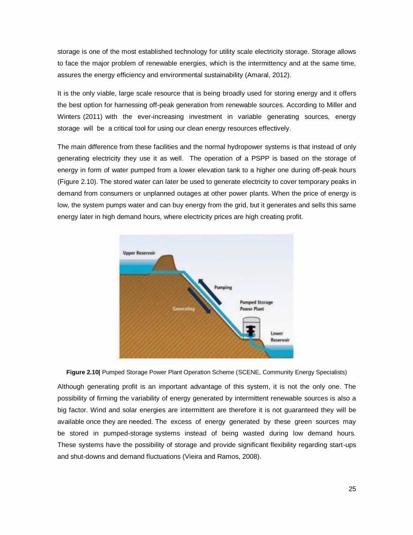
The main difference from these facilities and the normal hydropower systems is that instead of only

generating electricity they use it as well. The operation of a PSPP is based on the storage of

energy in form of water pumped from a lower elevation tank to a higher one during off-peak hours

(Figure 2.10). The stored water can later be used to generate electricity to cover temporary peaks in

demand from consumers or unplanned outages at other power plants. When the price of energy is

low, the system pumps water and can buy energy from the grid, but it generates and sells this same

energy later in high demand hours, where electricity prices are high creating profit.

Figure 2.10| Pumped Storage Power Plant Operation Scheme (SCENE, Community Energy Specialists)

Although generating profit is an important advantage of this system, it is not the only one. The

possibility of firming the variability of energy generated by intermittent renewable sources is also a

big factor. Wind and solar energies are intermittent are therefore it is not guaranteed they will be

available once they are needed. The excess of energy generated by these green sources may

be stored in pumped-storage systems instead of being wasted during low demand hours.

These systems have the possibility of storage and provide significant flexibility regarding start-ups

and shut-downs and demand fluctuations (Vieira and Ramos, 2008).

26

2.6. Optimization

2.6.1. Methods of optimization

The optimization is a tool that can aid the designer to more easily test changes in design variables

and quickly interpret their results until they reach a closest possible to the desired result. Through

mathematical models and numerical methods it is possible to obtain for a given project the best

results in a set of feasible alternatives by the evaluation of a function that represents the

optimization problem.

There are several techniques for optimizing an objective function for both a single-objective analysis

as to a multi-objective analysis. For a local optimization it is usually used a gradient method being

the sequential quadratic programming, SQP, an example, and for a global optimization, genetic

algorithms, GA, are another example. (Santos, 2009).

The advantages of the SQP focus on the fact that it is a technique already used successfully in

many fields and in particular in the conceptual optimization of axial turbines (Albuquerque 2006)

and axial compressors axial compressors in multiple stages (Sousa Junior, 2007).

The advantages of evolutionary algorithms (EA) such as GA is due to the fact that it is the most

appropriate technique (independent of the type of optimization problem) for solving problems goal-

single and multi-purposes, for maintaining a set of applicants in parallel (Khatib and Fleming, 1997).

There are numerous applications of evolutionary in various branches of engineering algorithms.

According to Sarker and Newton (2008) a general optimization problem can be classified as shown

in Figure 2.11.

Level 1

Level 2

Level 3

Level 4

General optimization problem

Single objective Multi-objectives

Without restrictions With restrictions

Continuous/discrete Continuous/real Mixed

27

Level 5

Figure 2.11| Classification of a optimization problem (based on Sarker and Newton, 2008)

Level 1 refers to the identification of the optimization problem, the level 2 to the classification of

objectives and the type of objective (maximization or minimization) and the level 3 to the

classification of the problem as well as restrictions. The level 4 of the scheme refers to the

classification of the variables used and at last level 5 refers to the classification of the objective

function. The above levels are important for proper modeling of the optimization problem

considered, in which the initial step can be considered the most important step in the optimization

process (Nocedal and Wright, 1999). A very simple model cannot give a full awareness of the

problem, but on the other hand, a very complex modeling can become very difficult problem to

solve.

2.6.2. Genetic algorithms

Regarding to optimization techniques, GA’s are almost among of all of them so they are the one

considered in this work. According to Costa et al. (2010), they are stochastic algorithms whose

search methods to model some natural phenomena: genetic inheritance and Darwinian strife for

survival. The concept of genetic algorithms was developed by Holland and his colleagues in the

1960s and 1970s. GA is inspired by the evolutionist theory explaining the origin of species. In

nature, weak and unfit species within their environment are faced with extinction by natural

selection. The strong ones have greater opportunity to pass their genes to future generations via

reproduction. In the long run, species carrying the correct combination in their genes become

dominant in their population. Sometimes, during the slow process of evolution, random changes

may occur in genes. If these changes provide additional advantages in the challenge for survival,

new species evolve from the old ones. Unsuccessful changes are eliminated by natural selection

(Konak et al., 2006). A genetic algorithm follows a step-by-step procedure schematized in Figure

2.12.

In GA terminology, a solution vector is called an individual or a chromosome. Chromosomes are

made of discrete units called genes. Each gene controls one or more features of the chromosome.

In the original implementation of GA by Holland, genes are assumed to be binary numbers. In later

implementations more varied gene types have been introduced. Normally, a chromosome

Linear or

non-linear

Convex or

non-convex

Differentiable or

non-differentiable

28

corresponds to a unique solution x in the solution space, being the solution space the total amount

of possible individuals. This depends on all the possible combination of chromosomes, i.e., the set

of all possible input permutations. Small variations in system complexity can greatly increase the

solution space. This requires a mapping mechanism between the solution space and the

chromosomes. This mapping is called an encoding. In fact, GA works on the encoding of a problem,

not on the problem itself (Michalewicz, 1996).

GA operates with a collection of chromosomes called a population. The population is normally

randomly initialized as seen in Figure 2.12. As the search evolves, the population includes fitter and

fitter solutions, and eventually it converges, meaning that it is dominated by a single solution. Thus,

there must also be constrains in the system to guide the evolution of the solutions. These

constrains are imposed to the algorithm and represent physical impositions. They define the

boundaries of the solutions’ evolution and determine its convergence towards a feasible solution,

through penalty factors associated with each violation that reduce the total fitness (Obitko, 1998).

There are also a certain number of initial parameters that can be tuned, prior to the simulation, that

affect the quality of the convergence.

29

Figure 2.12| Flowchart of the GA cycle (Lin, 2006)

GA use two operators to generate new solutions from existing ones: crossover and mutation. The

crossover operator is the most important operator of GA. In crossover generally two chromosomes

called parents are combined together to form new chromosomes called offspring. The parents are

selected among existing chromosomes in the population with preference towards fitness so that

offspring is expected to inherit good genes which make the parents fitter. By iteratively applying the

crossover operator, genes of good chromosomes are expected to appear more frequently in the

population, eventually leading to convergence to an overall good solution.

The mutation operator introduces random changes into characteristics of chromosomes. Mutation is

generally applied at the gene level. In typical GA implementations the mutation rate (probability of

changing the properties of a gene) is very small, typically less than 1% (Konak et al., 2006).

Therefore, the new chromosome produced by mutation will not be very different from the original

one. Mutation plays a critical role in GA. As discussed earlier, crossover leads the population to

30

converge by making the chromosomes in the population alike. Mutation reintroduces genetic

diversity back into the population and assists the search escape from local optima.

Reproduction involves selection of chromosomes for the next generation. In the most general case,

the fitness of an individual determines the probability of its survival for the next generation. There

are different selection procedures in GA depending on how the fitness values are used.

Besides all these parameters, in this type of algorithms the term elitism is also essential for a good

and fast approach. This term means that the best solution found so far during the search has

immunity against selection and always survives in the next generation. In this way an Elite

Population is a subgroup of individuals from each generation that represent the fittest solutions and

that are not subject to crossover passing directly onto the next generation. This particularity permit

to avoid the loss of the optimal solutions from each generation (Konak et al., 2006).

Optimization techniques have been used by hydraulic engineers for more than 40 years, in order to

project, plan and manage complex systems (Filho, 2006) occupying the optimization of

pump/turbine-operation with energy consumption/production an important role.

Coelho et al. (2012) developed several analysis of diverse optimization algorithms for pump

scheduling in water supply systems in which the optimization methods applied in the WSS obtained

success, presenting cost savings from 14% to 70%. In Allan et al. (2009) the best pump efficiency

solutions were analyzed developing a non-specific program that could calculate the optimum

number of pumps that should be running for any given system characteristics. In Gonçalves et al.

(2011) a best economical hybrid solution is applied and the study showed the installation of a micro

hydro in a real small water distribution system using water level controls and pump operation

optimization by using genetic algorithms shows the improvement of the energy efficiency in 63%.

31

3. CASE STUDY DESCRIPTION AND MODELLING

This chapter begins by presenting the two case studies analysed, the Beliche system and the case of

Socorridos pumped-storage hydropower plant, introducing data such as its location and geometric

and hydraulic characterization. Following it is presented the computational models developed for

each case and its components as well as the analyses that are assessed. For the case study of

Socorridos it is also presented the optimization procedure applied.

Content

3.1. Case Study A – Beliche System .................................................................................... 32

3.2. Case Study B – Socorridos Pumped-Storage System ................................................... 40

3

32

3.1. Case study A – Beliche system

3.1.1. System description

A real supply system is studied in order to optimize and evaluate the energy produced by hydraulic

turbines. It is utilized an operational research methodologies assisted by a hydraulic simulation

software that allows the modelling of a mathematical representation of the system. The analysis

focuses is an already existing water supply system with an integrated small hydropower plant and a

guaranteed discharge for the population with availability of potential energy that can be used locally

or to be sold to the national electric grid, depending on the tariff and the local advantages. The

hydropower plant is currently completed and running but their production needs improvement of

operation.

The supply system for this case study was chosen following the investigation of Livramento (2013)

and the publications of Carriço et al. (2013), Ramos et al. (2010) and Samora et al. (2013) under

TRUST subject. Their respective studies are essential to obtain the information and the best

knowledge of the case study.

The analyzed case study is the Eastbound system, a subsystem of the Multi-Municipal Water

Supply System (MMWSS) for the Algarve region in Portugal. Algarve region is the most popular

touristic destination in Portugal, receiving a high number of people at the summer season. MMWSS

supplies 450,000 inhabitants from October to May, value that almost triples in the high season.

MMWSS has four surface water sources (tanks): Odeleite/Beliche; Bravura; Funcho and Odelouca.

The Eastbound system is supplied by the Beliche dam that aims at irrigation and water consumption

uses and the water is treated in both Tavira and Beliche Water Treatment Plants (WTP). The raw

water main from Beliche to Tavira WTP has two pumping stations and at the upstream of Beliche

WTP there is a micro-hydropower plant (red circle in Figure 3.1) with an installed power of 11kW.

The real hydraulic circuit that is analyzed begins at the intake located at Beliche dam in Algarve

(South of Portugal) and continues until the WTP as showed in Figure 3.2.

The conveyance system of the water treatment plant is made of the following pressurized hydraulic

circuit that comprises of three branches:

From the intake tower of Beliche dam to pumping station which is composed of a tunnel

with 3.5 m in diameter and 390 m in longitudinal development;

From the pumping station to the branch section of WTP with 800 DN and longitudinal

development of 475 m;

33

From the branch section of the WTP to the entrance of the valve-chamber in the WTP, with

500 DN and longitudinal development of 455 m.

Figure 3.1| Operating scheme of the Eastbound system (Carriço et al., 2013)

Figure 3.2| View of Beliche Dam tank and treatment plant at Algarve (Ramos et al., 2010)

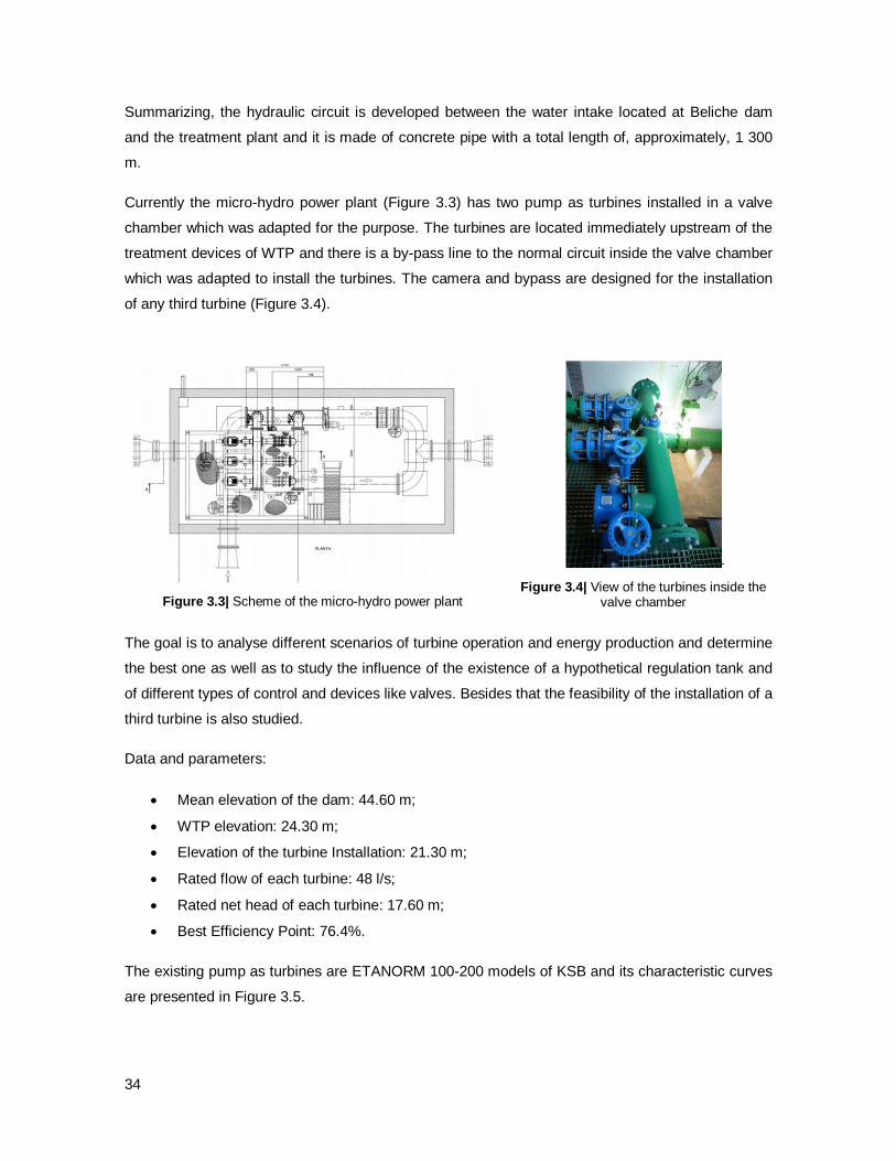
34

Summarizing, the hydraulic circuit is developed between the water intake located at Beliche dam

and the treatment plant and it is made of concrete pipe with a total length of, approximately, 1 300

m.

Currently the micro-hydro power plant (Figure 3.3) has two pump as turbines installed in a valve

chamber which was adapted for the purpose. The turbines are located immediately upstream of the

treatment devices of WTP and there is a by-pass line to the normal circuit inside the valve chamber

which was adapted to install the turbines. The camera and bypass are designed for the installation

of any third turbine (Figure 3.4).

Figure 3.3| Scheme of the micro-hydro power plant

Figure 3.4| View of the turbines inside the valve chamber

The goal is to analyse different scenarios of turbine operation and energy production and determine

the best one as well as to study the influence of the existence of a hypothetical regulation tank and

of different types of control and devices like valves. Besides that the feasibility of the installation of a

third turbine is also studied.

Data and parameters:

Mean elevation of the dam: 44.60 m;

WTP elevation: 24.30 m;

Elevation of the turbine Installation: 21.30 m;

Rated flow of each turbine: 48 l/s;

Rated net head of each turbine: 17.60 m;

Best Efficiency Point: 76.4%.

The existing pump as turbines are ETANORM 100-200 models of KSB and its characteristic curves

are presented in Figure 3.5.

35

(a) Characteristic curve

(b) Curve of the torque on the turbine shaft

(c) Curve of the turbine power

(d) Curve of the turbine efficiency

Figure 3.5| Turbine characteristic curves to 1500 rpm (50 Hz) (Livramento, 2013)

3.1.2. System modelling

The commercial hydraulic software used to model the system and perform the simulations is

Bentley’s WaterGEMS©. Figure 3.6 shows the scheme of the supply system analyzed. Beliche dam

is considered as tank with an elevation of 44.60 m from which the water is driven to the micro-hydro

power plant through a concrete pipe with a Hazen-Williams roughness factor of 110. The micro-

hydro power plant, and consequently, the two PAT, are represented by two turbines in parallel

(TBN-1 and TBN-2) whose characteristic head curve is shown in Figure 3.7 and adapted from

Livramento (2013).

36

Figure 3.6| Scheme of the Beliche system under analysis

Figure 3.7| Characteristic curve of each turbine (adapted from Livramento, 2013)

Downstream of the micro-hydro, and admitting that the head loss is negligible between these two

elements, there is a junction (WTP) with an elevation of 24.30 m which represents the Beliche WTP.

The model is designed as a bypass system controlled by a Throttle Control Valve (TCV-1) based on

head loss which ensures the water needs in the WTP when the demand is higher than the

maximum turbine flow. The bypass is only used when the flow treated is higher than 96 l/s which

corresponds to the maximum possible with two turbines and only with the amount of water

necessary to ensure the normal operation of the WTP.

It is assumed that the consumption of water in the system, i.e. the amount of water treated in the

WTP is imposed by the demand junction (WTP) and vary during the day as shown in Figure 3.8.

8

10

12

14

16

18

20

30 35 40 45 50

Net

Hea

d (m

)

Flow (l/s)

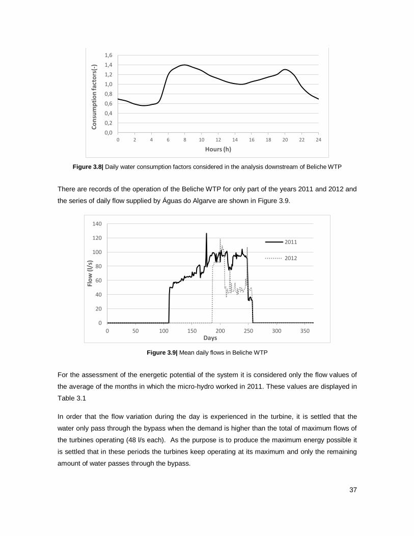
37

Figure 3.8| Daily water consumption factors considered in the analysis downstream of Beliche WTP

There are records of the operation of the Beliche WTP for only part of the years 2011 and 2012 and

the series of daily flow supplied by Águas do Algarve are shown in Figure 3.9.

Figure 3.9| Mean daily flows in Beliche WTP

For the assessment of the energetic potential of the system it is considered only the flow values of

the average of the months in which the micro-hydro worked in 2011. These values are displayed in

Table 3.1

In order that the flow variation during the day is experienced in the turbine, it is settled that the

water only pass through the bypass when the demand is higher than the total of maximum flows of

the turbines operating (48 l/s each). As the purpose is to produce the maximum energy possible it

is settled that in these periods the turbines keep operating at its maximum and only the remaining

amount of water passes through the bypass.

0,0

0,2

0,4

0,6

0,8

1,0

1,2

1,4

1,6

0 2 4 6 8 10 12 14 16 18 20 22 24

Co

nsu

mp

tio

n fa

cto

rs(-

)

Hours (h)

0

20

40

60

80

100

120

140

0 50 100 150 200 250 300 350

Flo

w (

l/s)

Days

2011

2012

38

Table 3.1| Mean daily flows, in 2011, in the months of operation of the micro-hydro

Month Mean Daily

Flow (l/s)

April 18.98

May 62.05

June 77.97

July 95.86

August 90.68

September 26.43

Average 62.00

Two options of turbines operation mode are considered: i) two turbines operating always with equal

flows and consequently with the same efficiency; ii) a second turbine only operating when the first

one is running at its maximum and if necessary.

Besides that is also considered different operating rules for energy production: iii) for all heads and

efficiencies values; iv) the energy for small heads and efficiency lower than 35% is neglected. The

purpose of the last suggestions iii) and iv) is to assess which one is more viable taking into account

the wear of the turbines. It is expected that the energy produced with efficiencies lower than 35%

would be very small, then the difference in terms of energy production between these two

conditions is also expected to be small. In this way the goal is to evaluate whether the fact that if

operating just for higher efficiencies or if the machines with no restrictions require a higher number

of star/stops of the turbine and consequently, excessive wear. The different hypotheses of turbine

operation and energy production are organized in scenarios presented in Table 3.2.

Table 3.2| Summary of the different scenarios analysed concerning the turbine operation and energy production

Scenario Turbine Operation Energy production

A Both turbines operating with equal flows and consequently with the same efficiency

All heads and efficiencies values

B One turbine at its maximum and the second one only when and if needed

All heads and efficiencies values

C Best turbine operation mode evaluate between A and B

High heads and efficiency higher than 35%

As previously mentioned, the power plant is prepared for the installation of a third turbine and the

viability of this decision is analyzed. In this case the bypass would be integrated just for demands

higher than 144 l/s because it corresponds the maximum turbine flow possible for three turbines.

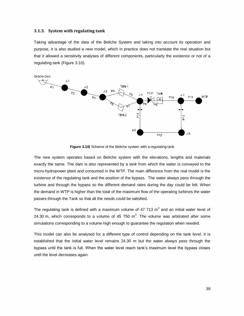
39

3.1.3. System with regulating tank

Taking advantage of the data of the Beliche System and taking into account its operation and

purpose, it is also studied a new model, which in practice does not translate the real situation but

that it allowed a sensitivity analyses of different components, particularly the existence or not of a

regulating tank (Figure 3.10).

Figure 3.10| Scheme of the Beliche system with a regulating tank

The new system operates based on Beliche system with the elevations, lengths and materials

exactly the same. The dam is also represented by a tank from which the water is conveyed to the

micro-hydropower plant and consumed in the WTP. The main difference from the real model is the

existence of the regulating tank and the position of the bypass. The water always pass through the

turbine and through the bypass so the different demand rates during the day could be felt. When

the demand in WTP is higher than the total of the maximum flow of the operating turbines the water

passes through the Tank so that all the needs could be satisfied.

The regulating tank is defined with a maximum volume of 47 713 m3 and an initial water level of

24.30 m, which corresponds to a volume of 45 750 m3. The volume was arbitrated after some

simulations corresponding to a volume high enough to guarantee the regulation when needed.

This model can also be analysed for a different type of control depending on the tank level. It is

established that the initial water level remains 24.30 m but the water always pass through the

bypass until the tank is full. When the water level reach tank’s maximum level the bypass closes

until the level decreases again.

40

3.1.4. Summary of analyses performed

In summary the study of the system of Beliche embraces the following analyses, schematized in

Figure 3.11:

The determination of the best scenario concerning turbine operation and energy

production;

The influence of the type of valves used for the system control;

The viability of the installation of a third turbine in the system;

The effect of a tank of regulation and a sensitivity analysis concerning:

o The influence of a control based on the water level of the regulation tank;

o The influence of the volume of the regulating tank;

Figure 3.11| Diagram of the Beliche system methodology

3.2. Case Study B – Socorridos pumped-storage system

3.2.1. System description

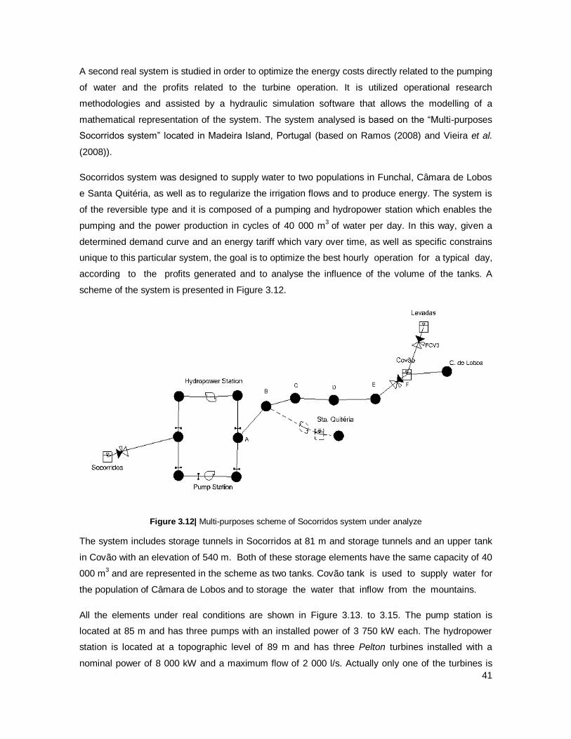
41

A second real system is studied in order to optimize the energy costs directly related to the pumping

of water and the profits related to the turbine operation. It is utilized operational research

methodologies and assisted by a hydraulic simulation software that allows the modelling of a

mathematical representation of the system. The system analysed is based on the “Multi-purposes

Socorridos system” located in Madeira Island, Portugal (based on Ramos (2008) and Vieira et al.

(2008)).

Socorridos system was designed to supply water to two populations in Funchal, Câmara de Lobos

e Santa Quitéria, as well as to regularize the irrigation flows and to produce energy. The system is

of the reversible type and it is composed of a pumping and hydropower station which enables the

pumping and the power production in cycles of 40 000 m3

of water per day. In this way, given a

determined demand curve and an energy tariff which vary over time, as well as specific constrains

unique to this particular system, the goal is to optimize the best hourly operation for a typical day,

according to the profits generated and to analyse the influence of the volume of the tanks. A

scheme of the system is presented in Figure 3.12.

Figure 3.12| Multi-purposes scheme of Socorridos system under analyze

The system includes storage tunnels in Socorridos at 81 m and storage tunnels and an upper tank

in Covão with an elevation of 540 m. Both of these storage elements have the same capacity of 40

000 m3 and are represented in the scheme as two tanks. Covão tank is used to supply water for

the population of Câmara de Lobos and to storage the water that inflow from the mountains.

All the elements under real conditions are shown in Figure 3.13. to 3.15. The pump station is

located at 85 m and has three pumps with an installed power of 3 750 kW each. The hydropower

station is located at a topographic level of 89 m and has three Pelton turbines installed with a

nominal power of 8 000 kW and a maximum flow of 2 000 l/s. Actually only one of the turbines is

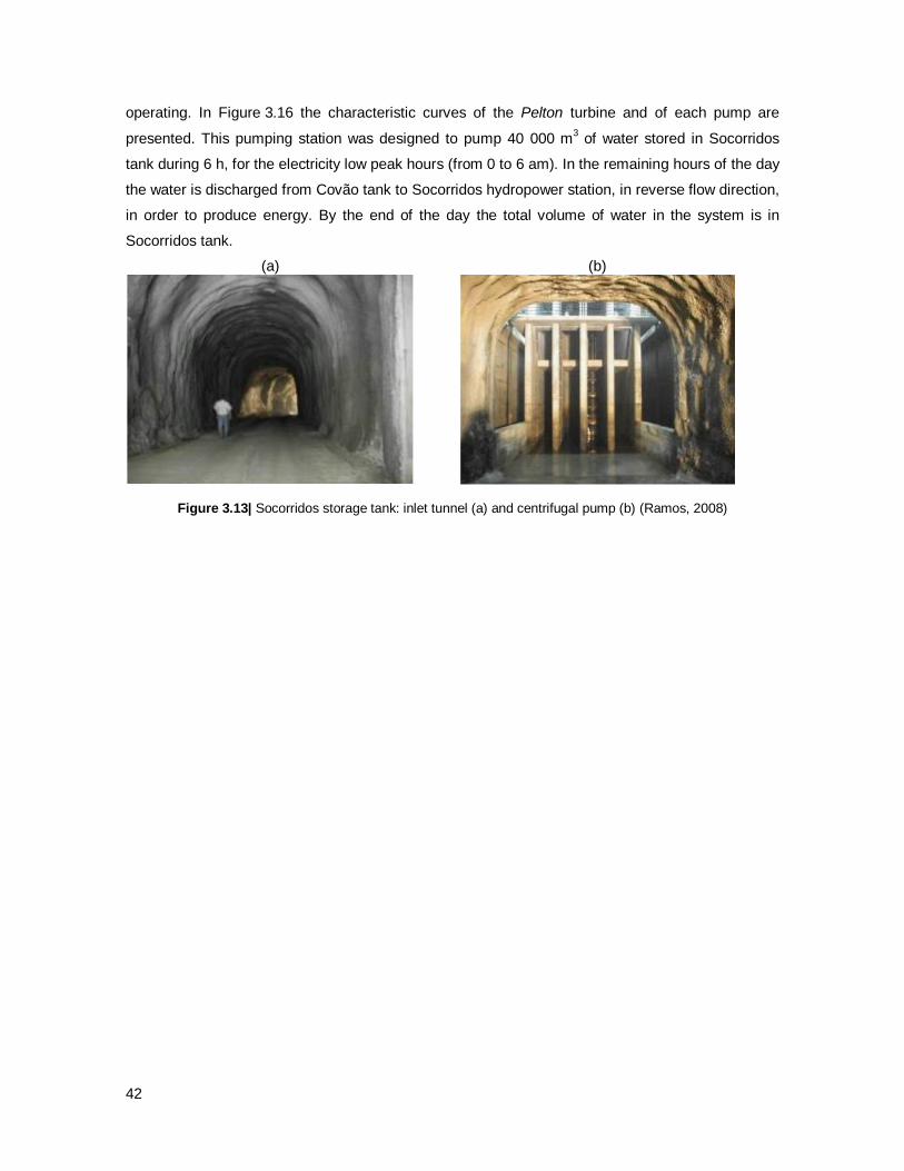
42

operating. In Figure 3.16 the characteristic curves of the Pelton turbine and of each pump are

presented. This pumping station was designed to pump 40 000 m3 of water stored in Socorridos

tank during 6 h, for the electricity low peak hours (from 0 to 6 am). In the remaining hours of the day

the water is discharged from Covão tank to Socorridos hydropower station, in reverse flow direction,

in order to produce energy. By the end of the day the total volume of water in the system is in

Socorridos tank.

(a)

(b)

Figure 3.13| Socorridos storage tank: inlet tunnel (a) and centrifugal pump (b) (Ramos, 2008)

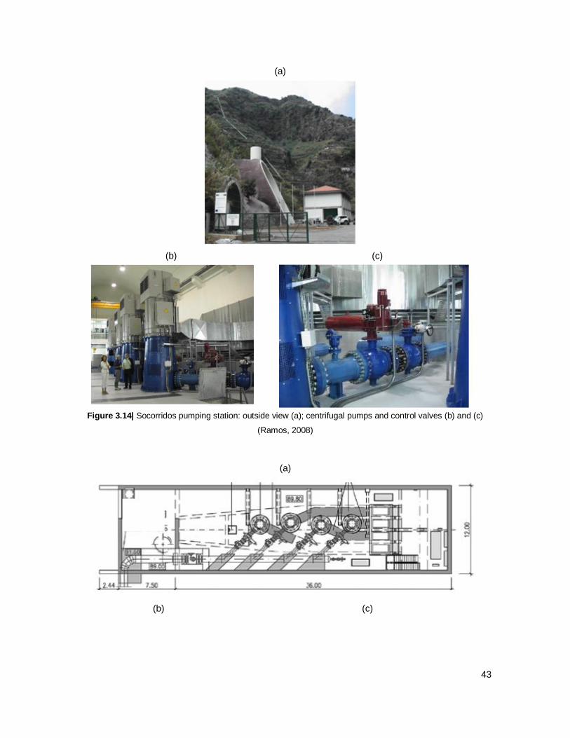
43

(a)

(b)

(c)

Figure 3.14| Socorridos pumping station: outside view (a); centrifugal pumps and control valves (b) and (c)

(Ramos, 2008)

(a)

(b) (c)

44

Figure 3.15| Socorridos pumping station: plant of the ground level (a), transversal view (b) and longitudinal

view (c) (Ramos, 2008)

Figure 3.16| Characteristic curves of the turbine (a) and of the pump (b) (adapted from Vieira et al. 2008)

At the downstream end of St. Quitéria pipe branch is located St. Quitéria hydropower plant and at

immediately downstream of it there is a water treatment plant and a storage-tank. This hydropower

station has a single Pelton turbine with a nominal flow rate of 1 m3/s and a bypass to the water

treatment plant (Figure 3.17).

0

100

200

300

400

500

600

700

0 1000 2000 3000

H (

m)

Q (l/s)

(a)

0

200

400

600

800

1000

0 200 400 600 800 1000

H (

m)

Q (l/s)

(b)

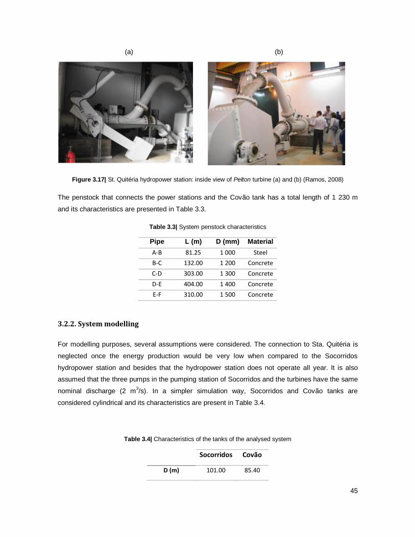
45

(a)

(b)

Figure 3.17| St. Quitéria hydropower station: inside view of Pelton turbine (a) and (b) (Ramos, 2008)

The penstock that connects the power stations and the Covão tank has a total length of 1 230 m

and its characteristics are presented in Table 3.3.

Table 3.3| System penstock characteristics

Pipe L (m) D (mm) Material

A-B 81.25 1 000 Steel

B-C 132.00 1 200 Concrete

C-D 303.00 1 300 Concrete

D-E 404.00 1 400 Concrete

E-F 310.00 1 500 Concrete

3.2.2. System modelling

For modelling purposes, several assumptions were considered. The connection to Sta. Quitéria is

neglected once the energy production would be very low when compared to the Socorridos

hydropower station and besides that the hydropower station does not operate all year. It is also

assumed that the three pumps in the pumping station of Socorridos and the turbines have the same

nominal discharge (2 m3/s). In a simpler simulation way, Socorridos and Covão tanks are

considered cylindrical and its characteristics are present in Table 3.4.

Table 3.4| Characteristics of the tanks of the analysed system

Socorridos Covão

D (m) 101.00 85.40

46

Min. Level (m) 0.5 0.5

Max level (m) 5.0 7.0

The water consumption in Câmara de Lobos follows the Manual of Basic Sanitation pattern (DGRN,

1991) and the inflow to Covão tank is assumed to have a constant value throughout the day. The

consumption in Câmara de Lobos and the discharge inlet in Covão tank for one day are displayed

in Figure 3.18.

Figure 3.18| Water volume consumption Câmara de Lobos and inlet volume in Covão

The electricity tariff used in this study, for the pumped-storage system is presented in Figure 3.19

and is based on the 2014 electricity tariff from Madeira Electricity Company (Appendix A.2) and

assumed to be equal in both cases of sale and purchase of energy.

Figure 3.19| Electricity tariff used in the model both for sale and purchase of energy (Eletricidade da Madeira)

3.2.3. Cost-effective optimization

3.2.3.1. Optimization procedure

0

5

10

15

20

25

30

35

0-1

1-2

2-3

3-4

4-5

5-6

6-7

7-8

8-9

9-10

10-1

1

11-1

2

12-1

3

13-1

4

14-1

5

15-1

6

16-1

7

17-1

8

18-1

9

19-2

0

20-2

1

21-2

2

22-2

3

23-2

4

Wat

er F

low

(l)

Time (h)

Consumption (Câmara de Lobos) Inflow (Covão)

0,00

0,02

0,04

0,06

0,08

0,10

0,12

0-1

1-2

2-3

3-4

4-5

5-6

6-7

7-8

8-9

9-10

10-1

1

11-1

2

12-1

3

13-1

4

14-1

5

15-1

6

16-1

7

17-1

8

18-1

9

19-2

0

20-2

1

21-2

2

22-2

3

23-2

4Elec

tric

ity

Pri

ce (

€/kW

h)

Time (h)

47

For the optimization of the pumps/turbines hourly operation a sequence of decisions along a day is

established in order to reduce the total costs and increase the total benefits related to the electricity

use. To minimize operation costs it is always preferable to pump during off-peak hours as the

energy cost of pumping the same volume can be as much as less than half the price. To maximize

the benefits in energy production it is preferable to turbine the water during these peak-hours. This

problem would be easy to solve if the Covão tank had enough volume to store water during these

off-peak hours, delivering it and allowing some volumes to return to Socorridos producing energy

during the peak consumption. Socorridos tank should also have enough volume to store the water

in the peak hours. Since the tanks capacity is limited the difficulty of the problem is increased and

some decisions have to be made.

The analysis is done in 24 h cycles with time steps of one hour. The goal is to achieve the best

solution for each hour considering that this action influences the next ones. It is analysed how the

system reacts to the pumping operation in each hour, guarantying the supply of water to the

populations and all the hydraulic restrictions. Consequently the turbine operation is also determined

and analysed.

An integrated software tool has been developed in MATLAB for determining the optimum pump and

turbine schedules and tanks water levels that minimize the pumping costs. This tool incorporates a

hydraulic simulator that describes the hydraulic behaviour of the system during 24 hour simulation

(EPANET) and an optimization solver based on an objective function to minimize. It is determined

the optimal solution without violating system constraints and ensuring that downstream demands

are satisfied. These constraints refer to the minimum and maximum allowable water levels in the

storage tanks and the imposition that the initial and the final tank levels match to ensure that each

daily cycle ended without volume variation. Therefore, the problem is solved in terms of the water

levels in the tanks.

The referenced study has cycles starting at 0:00 with the Socorridos tank full and the Covão at is

minimum (level of 0.5 m). This means that whatever happened during the rest of the simulation, in

the first hours of the day the pumps must be switched-on because Socorridos is already full and

cannot storage more water from the turbines and Covão is empty and needs flow to satisfy the

population needs, even if it meant operating at disadvantageous hours. In the same way, in the last

hours of the day the turbines must be operating because it is wanted to finish the simulation with

the same initial parameters.

The output of the optimization routines is introduced in EPANET to verify the hydraulic behaviour of

the system. For a simulation more realistic regarding the operating procedures it is inputted that the

system:

48

Switches on the pump if the water level in Covão tank is less than the minimum value;

Switches off the pump if the water level in Covão tank reach the maximum value;

Switches on the turbine if the pumps are off and vice-versa.

With that in mind an optimization program is developed with the objective function to minimize given

by equation 3.1.

The variables of the optimization are:

Electricity tariff associated with the pump operation (€/kWh) – 𝑐𝑃

Electricity tariff associated with the turbine operation (€/kWh) – 𝑐𝑇

Pump efficiency (-) – 𝜂𝑃

Turbine efficiency (-) - 𝜂𝑇

Water level raise or decrease in Covão tank (m) – 𝑑𝑁

This function represents the costs associated with the level variation either for pump or turbine

modes. If there is a raise in Covão tank water level (𝑑𝑁 > 0) the pump station is operating and has

a cost (𝑐𝑃) associated for each hour. On the other hand if there is a decrease in Covão tank

water level (𝑑𝑁 < 0) the system is discharging water from Covão to Socorridos and,

consequently, producing energy that can be sold at a price (𝑐𝑇). With this function is possible to

attribute the electricity costs for the pumping hours and the selling price for the electricity

production hours.

The reference system schedule is projected with an operation mode where the water pumping

occurs during the first six hours of the day (from 0 to 6 am) and in the remaining hours the

system produce energy by hydropower. This optimization approach is expected to output a new

pump/turbine schedule with no restriction related to pump and turbine hours and higher profits when

compared with the reference system.

3.2.3.2. Feasibility and constraint handling

In the literature of the pump scheduling problems, constraints are usually handled by means of

penalty functions.

𝑓 = ∑ [𝑐𝑃,ℎ

𝜂𝑃

. (𝑑𝑁ℎ + |𝑑𝑁ℎ|

2) + 𝑐𝑇,ℎ . 𝜂𝑇 . (

𝑑𝑁ℎ − |𝑑𝑁ℎ|

2)]

24

ℎ=1

(3.1)

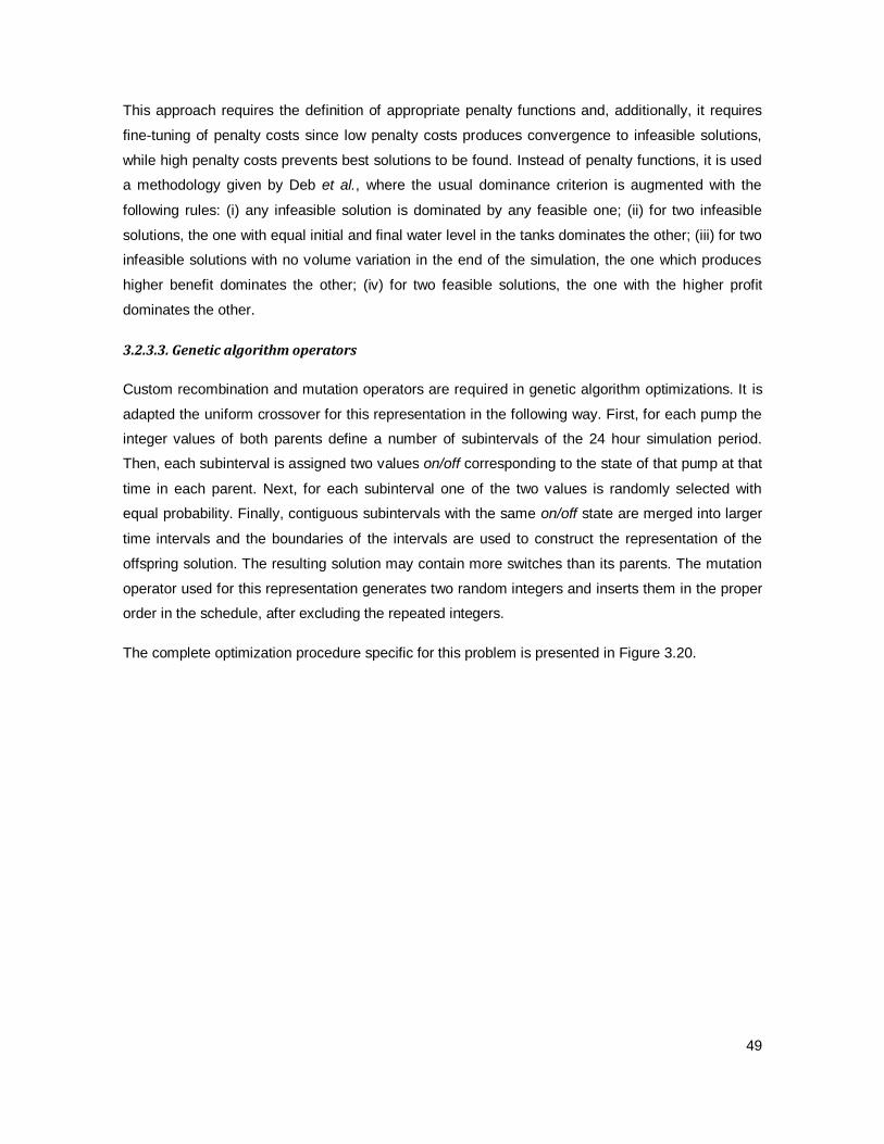
49

This approach requires the definition of appropriate penalty functions and, additionally, it requires

fine-tuning of penalty costs since low penalty costs produces convergence to infeasible solutions,

while high penalty costs prevents best solutions to be found. Instead of penalty functions, it is used

a methodology given by Deb et al., where the usual dominance criterion is augmented with the

following rules: (i) any infeasible solution is dominated by any feasible one; (ii) for two infeasible

solutions, the one with equal initial and final water level in the tanks dominates the other; (iii) for two

infeasible solutions with no volume variation in the end of the simulation, the one which produces

higher benefit dominates the other; (iv) for two feasible solutions, the one with the higher profit

dominates the other.

3.2.3.3. Genetic algorithm operators

Custom recombination and mutation operators are required in genetic algorithm optimizations. It is

adapted the uniform crossover for this representation in the following way. First, for each pump the

integer values of both parents define a number of subintervals of the 24 hour simulation period.

Then, each subinterval is assigned two values on/off corresponding to the state of that pump at that

time in each parent. Next, for each subinterval one of the two values is randomly selected with

equal probability. Finally, contiguous subintervals with the same on/off state are merged into larger

time intervals and the boundaries of the intervals are used to construct the representation of the

offspring solution. The resulting solution may contain more switches than its parents. The mutation

operator used for this representation generates two random integers and inserts them in the proper

order in the schedule, after excluding the repeated integers.

The complete optimization procedure specific for this problem is presented in Figure 3.20.

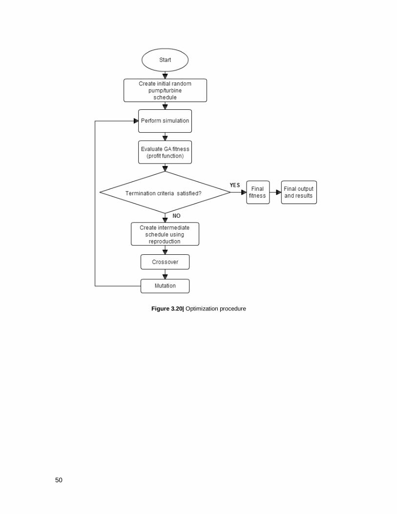
50

Figure 3.20| Optimization procedure

51

52

4. ANALYSES AND RESULTS

In this chapter the computational results for the scenarios and models studied are presented and

discussed. In the first part of the chapter an analysis on the best scenario for energy production and

operation of the turbines is made as well as an economic analysis concerning the placing of a third

turbine in the Beliche system. Following sensitivity analyses on the existence of a regulating and

different types of control tank are made. Finally, there is a presentation and discussion of results of

the best hourly operation for one day, according to the electricity tariff, for the Socorridos

system with water consumption and inlet discharge and a analysis on the influence of the volume of

the tanks.

Content

4.1. Case study A – Beliche system ..................................................................................... 53

4.2. Case study B – Pumped-storage Socorridos system ..................................................... 68

4

53

4.1. Case study A – Beliche system

4.1.1. Analyses of different scenarios

Taking into account the system of Beliche several simulations are performed for the scenarios of

turbine operation and energy production and for the different flows treated in the Beliche WTP. For

each situation the energy produced is obtained from equation (2.2).

Scenario A

The average energy produced, per day and per month, in each month of operation in 2011, in the

micro-hydro with the two turbines installed in parallel for the scenario A is shown in Table 4.1.

These calculations are also made for arbitrary flow values to a wider analysis.

Table 4.1| Mean of produced energy, in 2011, in the months of operation of the micro-hydro with 2 turbines installed considering them always performing at the same efficiency and for all head values and efficiencies

Month Mean Daily Flow (l/s)

Energy (kWh/day)

Energy (kWh/month)

April 18.98 0.0 0.0

May 62.05 88.9 2192.4

June 77.97 174.5 4303.1

July 95.86 237.3 5853.9

August 90.68 223.8 5520.3

September 26.43 0.0 0.0

Arbitrary Values

57.00 249.8 1656.7

100.00 290.0 6160.9

120.00 67.2 7153.1

Total 17.9 MWh

It is noticed that for demand flows like 18.98 and 26.43 l/s the flow values that passes in the

turbines are so low that they is not enough to produce energy. The total of energy produced in all

the 148 days of operation of the micro-hydro is equal to 17.9 MWh

Scenario B

In the same way, the correspondent energy production for the scenario B – starting a second

turbine only after the first one is at its maximum and if it is needed for all efficiency and head values

- is presented in Table 4.2.

54

The energy produced in the days of operation of the micro-hydro is equal to 22.6 MWh which is

higher than in scenario A. In this way, it is noted the condition of the turbine running at its maximum

efficiency and only resorting to the second turbine if needed and in the amount necessary is the

more profitable and it is the one to be taken into account in the calculations of scenario C.

Table 4.2| Mean of produced energy, in 2011, in the months of operation of the micro-hydro with 2 turbines installed considering one turbine at its maximum efficiency and the second only switched-on if needed.

Operation for all head and efficiency values

Month Mean Daily Flow (l/s)

Energy (kWh/day)

Energy (kWh/month)

April 18.98 5.7 141.1

May 62.05 151.3 3731.3

June 77.97 224.0 5524.8

July 95.86 257.6 6354.8

August 90.68 251.7 6207.9

September 26.43 25.9 639.2

Arbitrary Values

57.00 137.3 3387.1

100.00 260.8 6433.7

120.00 278.8 6877.5

Total 22.6 MWh

Scenario C

Similarly to the previous scenarios calculations, the average energy produced, per day, in each

month of operation in 2011, in the micro-hydro with the two turbines installed for the scenario C -

neglecting the energy for small heads values and efficiency lower than 35% and taking advantage

of the best modes of operation of the turbines is shown in Table 4.3.

As expected, the energy produced in each month with the condition of the turbines operation with

restrictions related to its efficiency is slightly lower than in the scenario B, being the total in all days

of operation of the micro-hydro equal to 22.1 MWh. Regarding the turbines wear, the number of

star/stops during one day is practically the same for all the flows analyzed (one/two starts and

stops) in the two scenarios. This similarity in the number of star/stops relates to the fact that for

flows in the range of 18 l/s the efficiency of the turbines reaches 0%, so the turbine also stops. In

this way, the mode of the turbines always working without restriction is the more feasible.

55

Table 4.3| Mean of produced energy, in 2011, in the months of operation of the micro-hydro with 2 turbines installed working if needed and neglecting the energy correspondent to small heads and efficiency values

lower than 35%

Month Mean Daily Flow (l/s)

Energy (kWh/day)

Energy (kWh/month)

April 18.98 1.6 38.3

May 62.05 147.0 3626.1

June 77.97 218.4 5387.7

July 95.86 257.2 6343.7

August 90.68 248.8 6137.4

September 26.43 24.8 612.1

Arbitrary Values

57.00 135.5 3342.2

100.00 260.7 6429.3

120.00 278.5 6868.3

Total 22.1 MWh

Assessment of the best scenario and influence of the type of valve

A summary of the energy produced in the 148 days of operation of the micro-hydro by the three

different scenarios is presented in Table 4.4.

Table 4.4| Summary of the energy produced in the 148 days of operation of the micro-hydro

Scenario Energy Produced (MWh)

A 17.9

B 22.6

C 22.1

Summarizing, scenario B is the most viable and is taken into account in further calculations.

The data flows available are only related to the energy consumption in the high season, i.e, in the

months of summer. It is known that in this area of Portugal, in summer the number of the population

increases a lot what is reflected in energy and water consumption. Due to the lack of data it is

admitted that in winter the energy production follows the same pattern than in the rest of the days of

utilization of the micro-hydropower plant which results in 55.8 MWh/year.

On the other hand, assuming that May can be considered as a representative month of the year,

once it presents a mean daily flow whose value is close to the monthly average (62 l/s), one obtains

a value of the total energy produced of approximately 55.2 MWh/year, very similar with the real one.

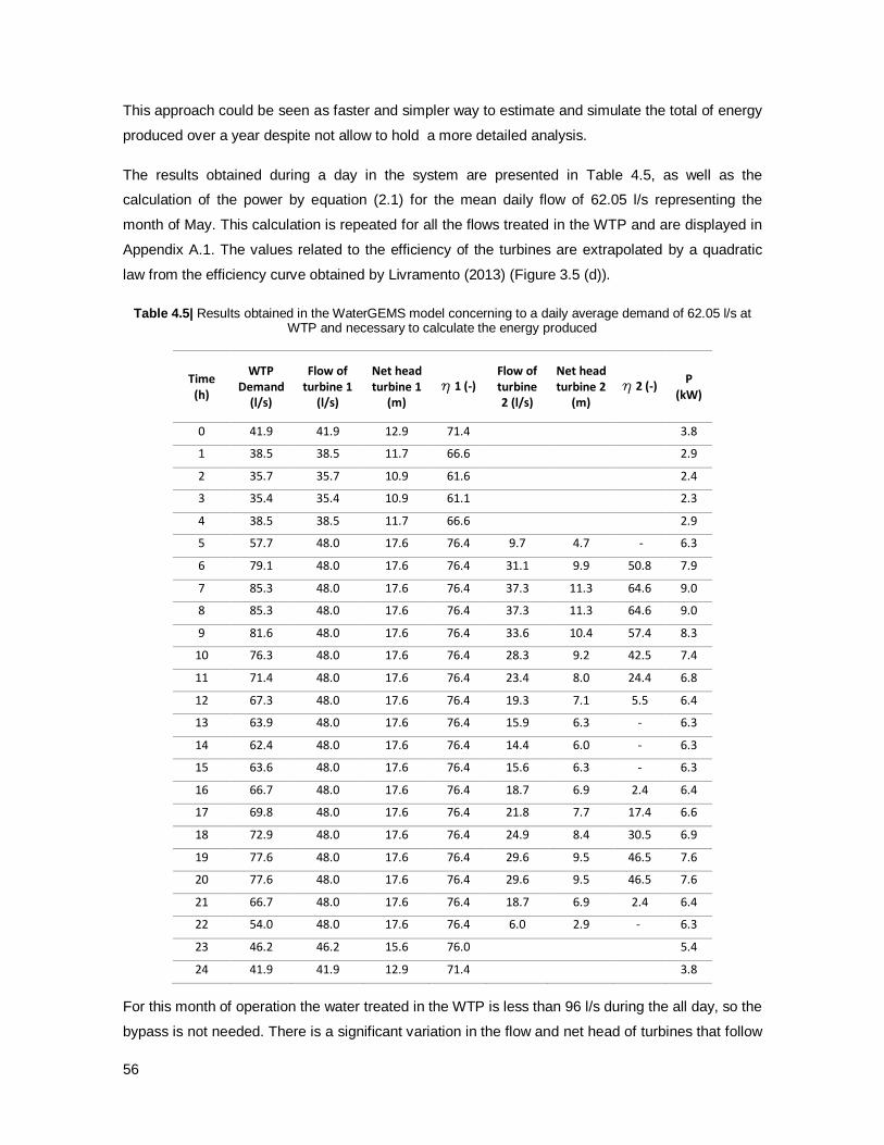
56

This approach could be seen as faster and simpler way to estimate and simulate the total of energy

produced over a year despite not allow to hold a more detailed analysis.

The results obtained during a day in the system are presented in Table 4.5, as well as the

calculation of the power by equation (2.1) for the mean daily flow of 62.05 l/s representing the

month of May. This calculation is repeated for all the flows treated in the WTP and are displayed in

Appendix A.1. The values related to the efficiency of the turbines are extrapolated by a quadratic

law from the efficiency curve obtained by Livramento (2013) (Figure 3.5 (d)).

Table 4.5| Results obtained in the WaterGEMS model concerning to a daily average demand of 62.05 l/s at WTP and necessary to calculate the energy produced

Time (h)

WTP Demand

(l/s)

Flow of turbine 1

(l/s)

Net head turbine 1

(m) η 1 (-)

Flow of turbine 2 (l/s)

Net head turbine 2

(m) η 2 (-)

P (kW)

0 41.9 41.9 12.9 71.4 3.8

1 38.5 38.5 11.7 66.6 2.9

2 35.7 35.7 10.9 61.6 2.4

3 35.4 35.4 10.9 61.1 2.3

4 38.5 38.5 11.7 66.6 2.9

5 57.7 48.0 17.6 76.4 9.7 4.7 - 6.3

6 79.1 48.0 17.6 76.4 31.1 9.9 50.8 7.9

7 85.3 48.0 17.6 76.4 37.3 11.3 64.6 9.0

8 85.3 48.0 17.6 76.4 37.3 11.3 64.6 9.0

9 81.6 48.0 17.6 76.4 33.6 10.4 57.4 8.3

10 76.3 48.0 17.6 76.4 28.3 9.2 42.5 7.4

11 71.4 48.0 17.6 76.4 23.4 8.0 24.4 6.8

12 67.3 48.0 17.6 76.4 19.3 7.1 5.5 6.4

13 63.9 48.0 17.6 76.4 15.9 6.3 - 6.3

14 62.4 48.0 17.6 76.4 14.4 6.0 - 6.3

15 63.6 48.0 17.6 76.4 15.6 6.3 - 6.3

16 66.7 48.0 17.6 76.4 18.7 6.9 2.4 6.4

17 69.8 48.0 17.6 76.4 21.8 7.7 17.4 6.6

18 72.9 48.0 17.6 76.4 24.9 8.4 30.5 6.9

19 77.6 48.0 17.6 76.4 29.6 9.5 46.5 7.6

20 77.6 48.0 17.6 76.4 29.6 9.5 46.5 7.6

21 66.7 48.0 17.6 76.4 18.7 6.9 2.4 6.4

22 54.0 48.0 17.6 76.4 6.0 2.9 - 6.3

23 46.2 46.2 15.6 76.0 5.4

24 41.9 41.9 12.9 71.4 3.8

For this month of operation the water treated in the WTP is less than 96 l/s during the all day, so the

bypass is not needed. There is a significant variation in the flow and net head of turbines that follow

57

the demand curve (Figure 3.8). It is also observed that by the end of 4 hours and after 22 h there is

only one turbine operating and in the remaining time the two of them. The operation of the second

turbine starts with flows higher than 48 l/s but in this case the energy is only produced between 6h

and 12 h and 16 h and 21 h due to the efficiency of the turbine for the respective flows reached 0%.

This situation of the number of turbines effectively producing energy, i.e., with efficiencies higher

than zero is easily evaluate in Figure 4.1. The blue columns represent the cases where the demand

flow is higher than 48 l/s which would switch on a second turbine and the orange columns represent

the number of turbines that effectively produce energy.

Figure 4.1| Comparison of the number of turbines theoretically operating based on the WTP flow and the ones

effectively producing energy based on its efficiency, in the month of May and for two turbines installed

For higher demand flows the use of bypass becomes more relevant since values higher than the

maximum possible flows in the turbines are reached and need to be controlled. A mean daily flow in

the WTP of 90.68 l/s corresponds to August as a month with significant consumption. The path of

the water in the system simulated in the model of WaterGems for this flow is shown in Figure 4.2.

It is visible that the flow in the WTP has the configuration of the daily water consumption curve

(Figure 3.8) and the flow in the turbine follows that same configuration whenever the demand is

lower than 96 l/s – which corresponds to the maximum flow with two turbines operating- otherwise it

remains around that value. The water only passes through the bypass in the periods with a demand

higher than 96 l/s and its amount is equivalent to the difference between the required treated water

and the maximum allowed to produce energy.

0

1

2

0 1 2 3 4 5 6 7 8 9 10 11 12 13 14 15 16 17 18 19 20 21 22 23 24Nu

mb

er o

f t

urb

ines

in o

pe

rati

on

Time (h) Turbines Operating Turbines Producing Energy

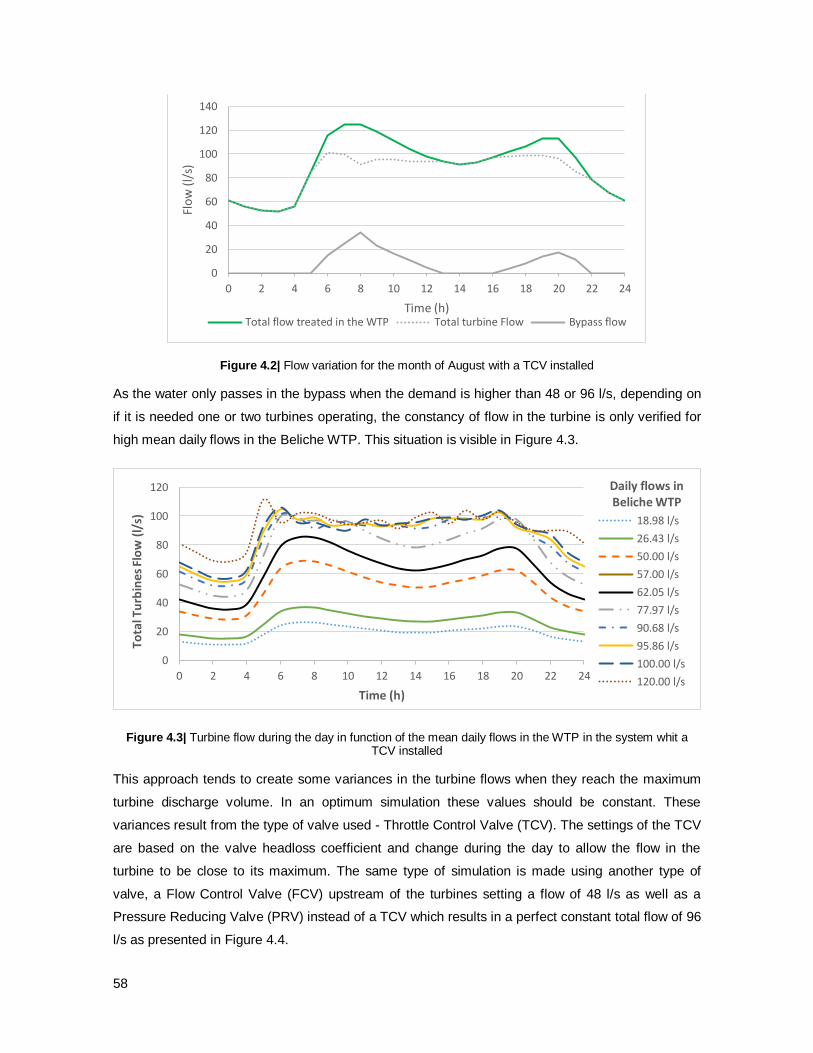
58

Figure 4.2| Flow variation for the month of August with a TCV installed

As the water only passes in the bypass when the demand is higher than 48 or 96 l/s, depending on

if it is needed one or two turbines operating, the constancy of flow in the turbine is only verified for

high mean daily flows in the Beliche WTP. This situation is visible in Figure 4.3.

Figure 4.3| Turbine flow during the day in function of the mean daily flows in the WTP in the system whit a TCV installed

This approach tends to create some variances in the turbine flows when they reach the maximum

turbine discharge volume. In an optimum simulation these values should be constant. These

variances result from the type of valve used - Throttle Control Valve (TCV). The settings of the TCV

are based on the valve headloss coefficient and change during the day to allow the flow in the

turbine to be close to its maximum. The same type of simulation is made using another type of

valve, a Flow Control Valve (FCV) upstream of the turbines setting a flow of 48 l/s as well as a

Pressure Reducing Valve (PRV) instead of a TCV which results in a perfect constant total flow of 96

l/s as presented in Figure 4.4.

0

20

40

60

80

100

120

140

0 2 4 6 8 10 12 14 16 18 20 22 24

Flo

w (

l/s)

Time (h) Total flow treated in the WTP Total turbine Flow Bypass flow

0

20

40

60

80

100

120

0 2 4 6 8 10 12 14 16 18 20 22 24

Tota

l Tu

rbin

es F

low

(l/

s)

Time (h)

Daily flows in Beliche WTP

18.98 l/s

26.43 l/s

50.00 l/s

57.00 l/s

62.05 l/s

77.97 l/s

90.68 l/s

95.86 l/s

100.00 l/s

120.00 l/s

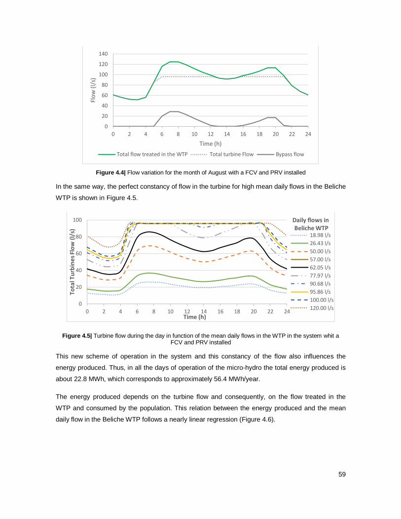
59

Figure 4.4| Flow variation for the month of August with a FCV and PRV installed

In the same way, the perfect constancy of flow in the turbine for high mean daily flows in the Beliche

WTP is shown in Figure 4.5.

Figure 4.5| Turbine flow during the day in function of the mean daily flows in the WTP in the system whit a FCV and PRV installed

This new scheme of operation in the system and this constancy of the flow also influences the

energy produced. Thus, in all the days of operation of the micro-hydro the total energy produced is

about 22.8 MWh, which corresponds to approximately 56.4 MWh/year.

The energy produced depends on the turbine flow and consequently, on the flow treated in the

WTP and consumed by the population. This relation between the energy produced and the mean

daily flow in the Beliche WTP follows a nearly linear regression (Figure 4.6).

0

20

40

60

80

100

120

140

0 2 4 6 8 10 12 14 16 18 20 22 24

Flo

w (

l/s)

Time (h)

Total flow treated in the WTP Total turbine Flow Bypass flow

0

20

40

60

80

100

0 2 4 6 8 10 12 14 16 18 20 22 24

Tota

l Tu

rbin

es F

low

(l/

s)

Time (h)

Daily flows in Beliche WTP

18.98 l/s

26.43 l/s

50.00 l/s

57.00 l/s

62.05 l/s

77.97 l/s

90.68 l/s

95.86 l/s

100.00 l/s

120.00 l/s

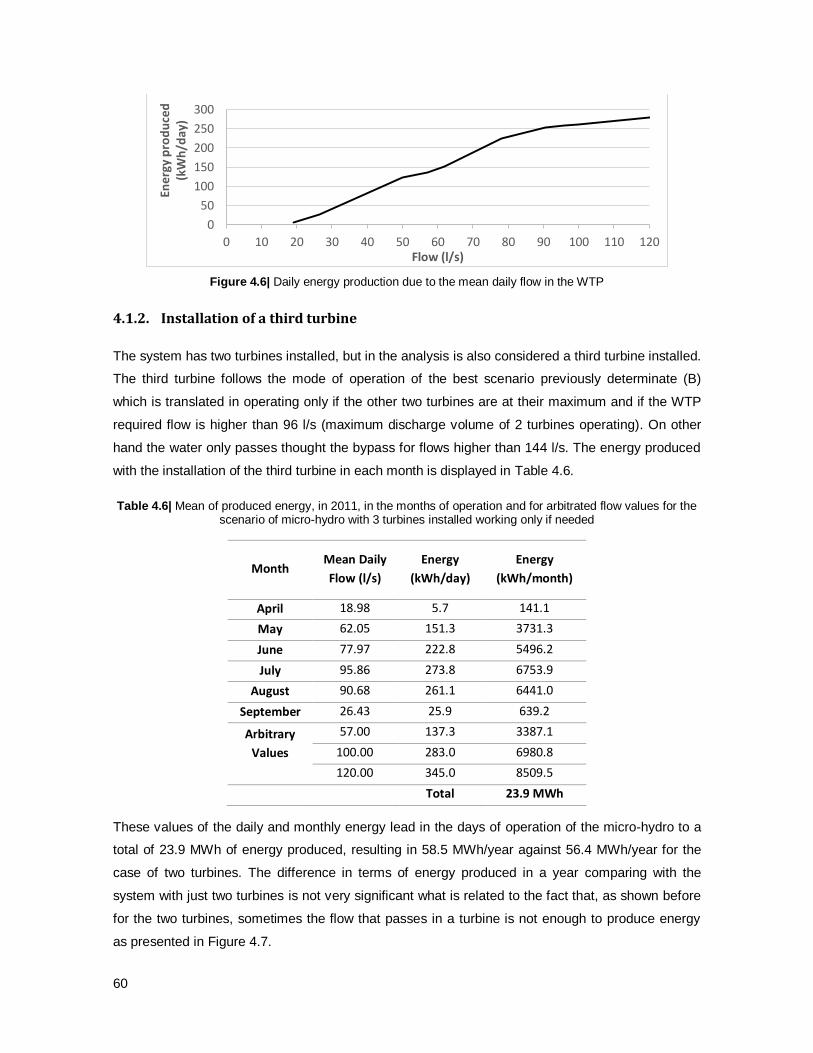
60

Figure 4.6| Daily energy production due to the mean daily flow in the WTP

4.1.2. Installation of a third turbine

The system has two turbines installed, but in the analysis is also considered a third turbine installed.

The third turbine follows the mode of operation of the best scenario previously determinate (B)

which is translated in operating only if the other two turbines are at their maximum and if the WTP

required flow is higher than 96 l/s (maximum discharge volume of 2 turbines operating). On other

hand the water only passes thought the bypass for flows higher than 144 l/s. The energy produced

with the installation of the third turbine in each month is displayed in Table 4.6.

Table 4.6| Mean of produced energy, in 2011, in the months of operation and for arbitrated flow values for the scenario of micro-hydro with 3 turbines installed working only if needed

Month Mean Daily

Flow (l/s)

Energy

(kWh/day)

Energy

(kWh/month)

April 18.98 5.7 141.1

May 62.05 151.3 3731.3

June 77.97 222.8 5496.2

July 95.86 273.8 6753.9

August 90.68 261.1 6441.0

September 26.43 25.9 639.2

Arbitrary

Values

57.00 137.3 3387.1

100.00 283.0 6980.8

120.00 345.0 8509.5

Total 23.9 MWh

These values of the daily and monthly energy lead in the days of operation of the micro-hydro to a

total of 23.9 MWh of energy produced, resulting in 58.5 MWh/year against 56.4 MWh/year for the

case of two turbines. The difference in terms of energy produced in a year comparing with the

system with just two turbines is not very significant what is related to the fact that, as shown before

for the two turbines, sometimes the flow that passes in a turbine is not enough to produce energy

as presented in Figure 4.7.

0

50

100

150

200

250

300

0 10 20 30 40 50 60 70 80 90 100 110 120

Ener

gy p

rod

uce

d

(kW

h/d

ay)

Flow (l/s)

61

Figure 4.7| Comparison of the number of turbines theoretically operating based on the WTP flow and the ones effectively producing energy based on the efficiency characteristic curve, in August and for three turbines

installed

4.1.3. Economic Analysis

The economic analysis of the operation of micro-hidropower plant considered two distinct

remuneration schemes: sale of the produced energy and consumption in-situ. For the first scheme

it is taken into account the energetic tariffs and the restrictions related to the Portuguese program of

micro-generation and presented in 2.4.2. For the scheme of consumption in-situ the remuneration is

calculated from the average rate of purchase from the data provided by the Entidade Reguladora

dos Serviços Energéticos (ERSE) relating to the transitional rate of sales to final customers in

medium voltage. It is estimated an average tariff of € 118.9/MWh for the year of 2014.

Given the lack of information on costs of the hydropower equipment it is considered estimated

values based on the study of Ramos and Ramos (2010). In this study the variation of the acquisition

costs of a turbine or a PAT is given by Figure 4.8.

Figure 4.8| Curves for the hydropower equipment initial cost - pump operating as a turbine and water turbine (adapted from Ramos e Ramos, 2010)

0

1

2

3

0 1 2 3 4 5 6 7 8 9 10 11 12 13 14 15 16 17 18 19 20 21 22 23 24Nu

mb

er o

f tu

rbin

es in

op

erat

ion

Time (h) Turbines Operating Turbines Effectively Operating

0

1000

2000

3000

4000

5000

6000

0 100 200 300

€ (

kW)

Power (kW)

Pump as Turbine

Turbine

62

Knowing the installed power of the two turbines is about 11 kW it is admitted a charge of 30 000 €

for the purchase and installation of the PATs in the referenced situation. Regarding the

maintenance cost during the period of analysis it is considered 2% of the installation costs. The

economic analysis is performed assuming constant prices and different discount rates for a period

of 15 years. The Net Present Value (NPV) and Benefit-Cost Ratio are calculated for three discount

rates (2%, 4% and 6%) and the Internal Rate of Return (IRR) is determined also for the period of 15

years. Although the long-term profitability of the general regime is similar or even superior to

subsidized regime it has a payback period of investment longer (Portal Energia, 2013) so the

subsidized regime is the one considered in the calculation of profit.

The results of the referenced scenario with two installed turbines in the micro-hydropower plant for

the two schemes of remuneration considering the production only in high season (i.e. in the 148

days of operation) or during all year are present in Table 4.7.

Table 4.7| Economic analysis of the existing scenario of two installed turbines in the micro-hydropower plant for the two schemes of remuneration

Sale Consumption in-situ

Production only in high season

Production all year Production only in

high season Production all year

IRR (%) 3.8% 17.7% 3.2% 16.8%

r (%) 2.0% 4.0% 6.0% 2.0% 4.0% 6.0% 2.0% 4.0% 6.0% 2.0% 4.0% 6.0%

NPV (1000€)

5.1 -0.4 -5.0 58.4 45.8 35.3 3.3 -1.9 -6.3 54.1 42.0 32.0

BCR (-)

1.17 0.99 0.84 2.91 2.47 2.11 1.11 0.94 0.80 2.77 2.35 2.01

It is visible that the production only in high season is not feasible once the 15 years taken into

account are not enough to the benefits equalize or exceed the costs for the discount rates of 4 and

6% which is also visible by the BCR lower than 1 for both sale and consumption in-situ.

In order to better understand the influence of the treated flow in the hydropower plant profitability it

is performed an economic analysis for the arbitrated flow values of 100 and 120 l/s that are

displayed in Table 4.8.

63

Table 4.8| Economic analysis of the existing scenario of two installed turbines in the micro-hydropower plant for the two schemes of remuneration and for arbitrated flow values

Sale Consumption in-situ Sale Consumption in-situ

Flow (l/s)

100 120

IRR (%) 29.4% 28.2% 31.2% 29.8%

r (%) 2.0% 4.0% 6.0% 2.0% 4.0% 6.0% 2.0% 4.0% 6.0% 2.0% 4.0% 6.0%

NPV (1000€)

121.7 100.5 83.1 114.2 94.0 77.5 132.2 109.6 91.1 124.3 102.7 85.1

BCR (-) 4.98 4.22 3.61 4.73 4.01 3.44 5.32 4.51 3.87 5.06 4.29 3.68

In the same way an economic analysis is made for the hypothesis of the installation of a third

turbine. Given that the hydromechanical equipment is installed in an existing chamber, not

requiring high costs of construction and once the installed power remained the same and the

information provided is not accurate it is considered the same initial costs. On other way in order to

bridge the initial costs expected in the installation of an extra turbine it is considered the

maintenance costs of 4% of the initial costs. The results are presented in Table 4.9.

Table 4.9| Economic analysis of the installation of a third turbine in the micro-hydropower plant for the two schemes of remuneration

Sale Consumption in-situ

Production only in

high season Production all year

Production only in high season

Production all year

IRR (%) 4.2% 18.2% 3.5% 17.3%

r (%) 2.0% 4.0% 6.0% 2.0% 4.0% 6.0% 2.0% 4.0% 6.0% 2.0% 4.0% 6.0%

NPV (1000 €)

6.2 0.5 -4.3 62.1 48.8 37.9 4.4 -1.2 -5.7 57.5 44.9 34.5

BCR (-) 1.20 1.01 0.86 3.03 2.56 2.19 1.14 0.96 0.82 2.88 2.44 2.08

It is visible that for this set of initial parameters and mean daily flows and taking in consideration the

energy production calculations, the installation of a third turbine is viable also only for the production

during all year. Thus, and likewise the case of two turbines, the analysis is extended to hypothetical

treated flow values of 100 and 120 l/s. The results are showed in Table 4.10. For all the flows

analyzed, the NPV, BCR and IRR values are higher for the case of an extra turbine in the system.

Although the differences are not very high, it reflects a possible improvement in the system.

64

Table 4.10| Economic analysis of the hypothesis of the installation of a third turbine in the micro-hydropower plant for the two schemes of remuneration and for arbitrated flow values

Sale Consumption in-situ Sale Consumption in-situ

Flow (l/s)

100 120

IRR (%) 30.8% 29.5% 35.5% 34.1%

r (%) 2.0% 4.0% 6.0% 2.0% 4.0% 6.0% 2.0% 4.0% 6.0% 2.0% 4.0% 6.0%

NPV

(1000 €) 132.6 109.9 91.2 124.6 102.9 85.2 163.0 136.1 114.2 153.5 127.9 107.0

BCR (-) 5.33 4.52 3.87 5.07 4.30 3.68 6.33 5.36 4.59 6.01 5.10 4.36

The comparison of the cases of two or three turbines installed in the hydropower plant for the

discount rate of 4 % are present in Figure 4.9 taking into account the two different remuneration

schemes: sale to the national electric grid (a) and consumption in-situ (b).

Figure 4.9| Comparison of the economic analysis of two and three turbines installed in the Beliche hydropower plant for a period of 15 years and a discount rate of 4% for the remuneration scheme of sale (a) and

consumption in-situ (b).

It is visible that both graphs follow the same configuration which results from the calculations in the

basis of the remuneration schemes being similar with the difference of higher NPV in the scheme of

sale to the national electric grid.

A more comprehensive comparison of the economic analysis for the different discount rates studies

is present in Figure 4.10. It is observed the scheme of sale to the national electric grid which

-40

-20

0

20

40

60

80

100

120

140

1 2 3 4 5 6 7 8 9 10 11 12 13 14 15

NP

V (

1000

€)

Years

(a)

-40

-20

0

20

40

60

80

100

120

140

1 2 3 4 5 6 7 8 9 10 11 12 13 14 15

NP

V (

1000

€)

Years

(b)

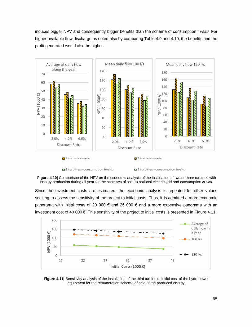
65

induces bigger NPV and consequently bigger benefits than the scheme of consumption in-situ. For

higher available flow discharge as noted also by comparing Table 4.9 and 4.10, the benefits and the

profit generated would also be higher.

Figure 4.10| Comparison of the NPV on the economic analysis of the installation of two or three turbines with energy production during all year for the schemes of sale to national electric grid and consumption in-situ

Since the investment costs are estimated, the economic analysis is repeated for other values

seeking to assess the sensitivity of the project to initial costs. Thus, it is admitted a more economic

panorama with initial costs of 20 000 € and 25 000 € and a more expensive panorama with an

investment cost of 40 000 €. This sensitivity of the project to initial costs is presented in Figure 4.11.

Figure 4.11| Sensitivity analysis of the installation of the third turbine to initial cost of the hydropower equipment for the remuneration scheme of sale of the produced energy

0

10

20

30

40

50

60

70

2,0% 4,0% 6,0%

NP

V (1

000 €)

Discount Rate

Average of daily flow along the year

0

20

40

60

80

100

120

140

2,0% 4,0% 6,0%

NP

V (1

000€)

Discount Rate

Mean daily flow 100 l/s

0

20

40

60

80

100

120

140

160

180

2,0% 4,0% 6,0%

NP

V (1

000 €)

Discount Rate

Mean daily flow 120 l/s

0

50

100

150

200

17 22 27 32 37 42

NP

V (

100

0 €

)

Initial Costs (1000 €)

Average ofdaily flow ina year

100 l/s

120 l/s

66

4.1.4. System with regulating tank

Several sensitivity analyses are carried out. A new model concept of the Beliche system (proposed

in 3.1.3) with two turbines installed and with a regulating tank is considered and it produced results

quite similar from the referenced system. The values of the total flows in the turbines suffer

significant variations during the day as presented in Figure 4.12.

Figure 4.12| Variation of the turbine flow during the day in function of the demand at the WTP

As it is expected the configuration of the flow load curve along the day tends to adopt the same

configuration as the daily water consumption factors curve. For high flows, i.e. when the demand

flows are greater than 96 l/s, the turbine flow remains constant since it is the best efficiency point.

It is also noted that the Figure 4.12 has a configuration quite similar to the Figure 4.3, 4.4. and 4.5.

The energy produced along one year with this new model and operation rules is 56.7 MWh which is

also very similar to the referenced studied model. This means the new solution also could be

adapted for the Beliche system if a regulating tank was involved with the advantage of a possibility

of implementation of different types of control.

Control based on the tank water level

For the simulation of the behavior of the system depending on the tank level, i.e. the bypass closes

when the water level reaches tank’s maximum and remains that way until the level decreases

again, the energy produced is presented in Table 4.11.

There is much more energy produced than in the previous analyzed simulations with a total of

32 MWh in the 148 days of operation and 80 MWh in the whole year. The disparity of energy

produced when compared with the model only resorting to the tank when needed is related to the

fact that now the turbines are always working at its maximum efficiency until the tank is full.

0

20

40

60

80

100

120

0 2 4 6 8 10 12 14 16 18 20 22 24

Tota

l Tu

rbin

e F

low

(l/

s)

Time (h)

Mean Daily flows at Beliche WTP

18.98 l/s

26.43 l/s

50.00 l/s

57.00 l/s

62.05 l/s

77.97 l/s

90.68 l/s

95.86 l/s

100.00 l/s

120.00 l/s

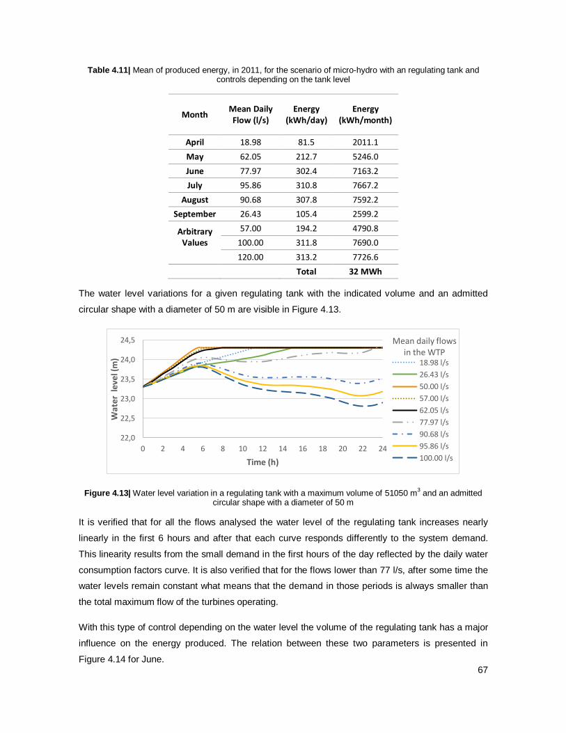
67

Table 4.11| Mean of produced energy, in 2011, for the scenario of micro-hydro with an regulating tank and controls depending on the tank level

Month Mean Daily Flow (l/s)

Energy (kWh/day)

Energy (kWh/month)

April 18.98 81.5 2011.1

May 62.05 212.7 5246.0

June 77.97 302.4 7163.2

July 95.86 310.8 7667.2

August 90.68 307.8 7592.2

September 26.43 105.4 2599.2

Arbitrary Values

57.00 194.2 4790.8

100.00 311.8 7690.0

120.00 313.2 7726.6

Total 32 MWh

The water level variations for a given regulating tank with the indicated volume and an admitted

circular shape with a diameter of 50 m are visible in Figure 4.13.

Figure 4.13| Water level variation in a regulating tank with a maximum volume of 51050 m3 and an admitted

circular shape with a diameter of 50 m

It is verified that for all the flows analysed the water level of the regulating tank increases nearly

linearly in the first 6 hours and after that each curve responds differently to the system demand.

This linearity results from the small demand in the first hours of the day reflected by the daily water

consumption factors curve. It is also verified that for the flows lower than 77 l/s, after some time the

water levels remain constant what means that the demand in those periods is always smaller than

the total maximum flow of the turbines operating.

With this type of control depending on the water level the volume of the regulating tank has a major

influence on the energy produced. The relation between these two parameters is presented in

Figure 4.14 for June.

22,0

22,5

23,0

23,5

24,0

24,5

0 2 4 6 8 10 12 14 16 18 20 22 24

Wat

er l

evel

(m

)

Time (h)

Mean daily flows in the WTP

18.98 l/s

26.43 l/s

50.00 l/s

57.00 l/s

62.05 l/s

77.97 l/s

90.68 l/s

95.86 l/s

100.00 l/s

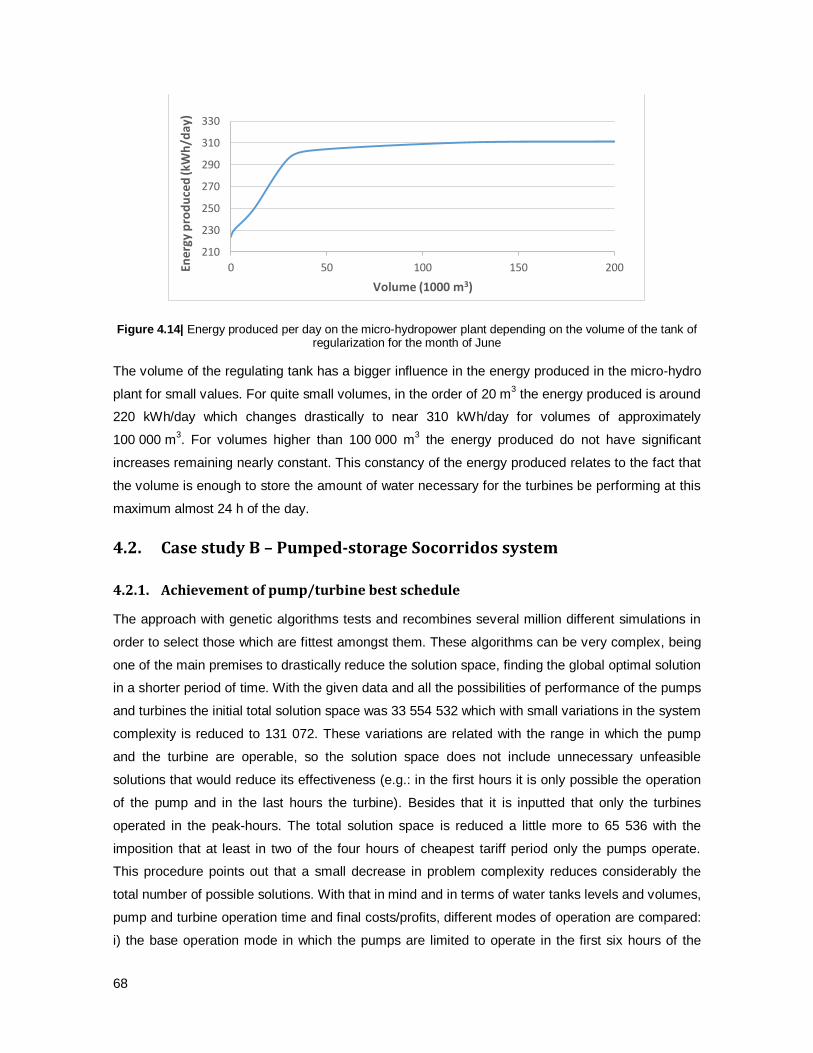
68

Figure 4.14| Energy produced per day on the micro-hydropower plant depending on the volume of the tank of regularization for the month of June

The volume of the regulating tank has a bigger influence in the energy produced in the micro-hydro

plant for small values. For quite small volumes, in the order of 20 m3 the energy produced is around

220 kWh/day which changes drastically to near 310 kWh/day for volumes of approximately

100 000 m3. For volumes higher than 100 000 m

3 the energy produced do not have significant

increases remaining nearly constant. This constancy of the energy produced relates to the fact that

the volume is enough to store the amount of water necessary for the turbines be performing at this

maximum almost 24 h of the day.

4.2. Case study B – Pumped-storage Socorridos system

4.2.1. Achievement of pump/turbine best schedule

The approach with genetic algorithms tests and recombines several million different simulations in

order to select those which are fittest amongst them. These algorithms can be very complex, being

one of the main premises to drastically reduce the solution space, finding the global optimal solution

in a shorter period of time. With the given data and all the possibilities of performance of the pumps

and turbines the initial total solution space was 33 554 532 which with small variations in the system

complexity is reduced to 131 072. These variations are related with the range in which the pump

and the turbine are operable, so the solution space does not include unnecessary unfeasible

solutions that would reduce its effectiveness (e.g.: in the first hours it is only possible the operation

of the pump and in the last hours the turbine). Besides that it is inputted that only the turbines

operated in the peak-hours. The total solution space is reduced a little more to 65 536 with the

imposition that at least in two of the four hours of cheapest tariff period only the pumps operate.

This procedure points out that a small decrease in problem complexity reduces considerably the

total number of possible solutions. With that in mind and in terms of water tanks levels and volumes,

pump and turbine operation time and final costs/profits, different modes of operation are compared:

i) the base operation mode in which the pumps are limited to operate in the first six hours of the

210

230

250

270

290

310

330

0 50 100 150 200Ene

rgy

pro

du

ced

(kW

h/d

ay)

Volume (1000 m3)

69

day; ii) the optimized operation mode in which the schedule of the pumps and turbines have no

restrictions.

Base operation mode

In Figure 4.15, the discharge volumes through the analysis of water levels in Socorridos and Covão

tanks are presented. It can be seen the initial and final water levels are imposed to be the same.

0

1

2

3

4

5

6

7

0 2 4 6 8 10 12 14 16 18 20 22 24

Wat

er le

vel (

m)

Co

vão

Time (h)

(a)

0

1

2

3

4

5

0 2 4 6 8 10 12 14 16 18 20 22 24

Wat

er le

vel (

m)

Soco

rrid

os

Time (h)

(b)

70

Figure 4.15| Water level variation in Covão (a) and Socorridos (b) tanks for the base mode of operation of the system and identification of the electricity tariff

The pumping and turbine operation time for each hour along the day are presented in Figure 4.16.

Figure 4.16| Pump and turbine operation time for the base mode of operation of the system

It can be seen for this mode of operation the pump station only operates during the first six hours of

the day as intended, while in the remaining time the hydropower station is working. In the last four

hours of the day the Covão tank has reached the minimum water level so there is no more water

available to turbine.

Optimized operation mode

In the same way the optimized solution for an operation without schedule limitations regarding the

water level of the tanks during the day, is presented in Figure 4.17.

In terms of the time of operation of the pumps and the turbines, Figure 4.18 shows the

correspondent best solution. In this case it the pumps usually operate during the 60 min in each

0,00

0,02

0,04

0,06

0,08

0,10

0,12

0 1 2 3 4 5 6 7 7 8 9 10 11 12 13 14 14 15 15 16 17 18 19 20 21 22 23 24

Ele

tric

ity

tari

ff (

€/K

wh

)

Time (h)

(c)

0

10

20

30

40

50

60

0 1 2 3 4 5 6 7 8 9 10 11 12 13 14 15 16 17 18 19 20 21 22 23 24

Mac

hin

e O

per

ati

ng

Tim

e (m

in)

Time (h)

Pump Turbine

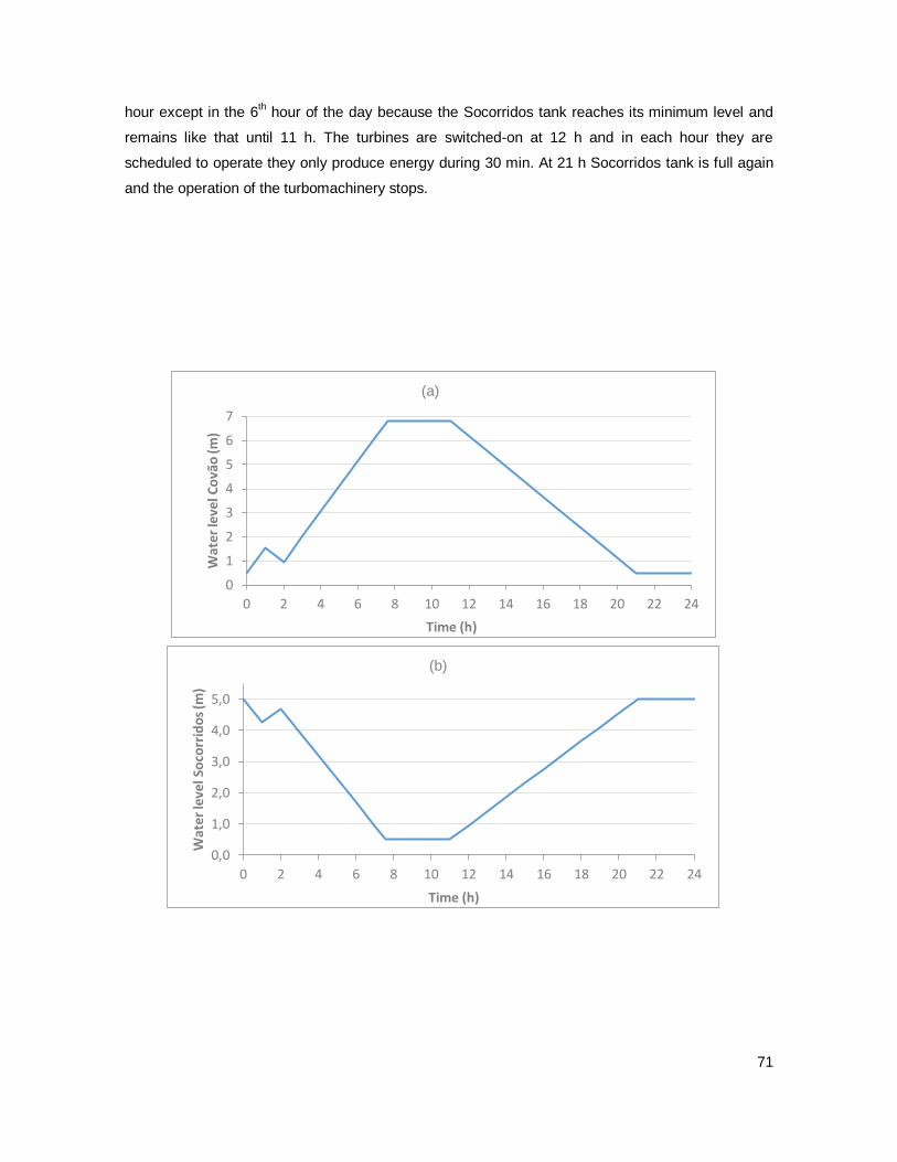
71

hour except in the 6th hour of the day because the Socorridos tank reaches its minimum level and

remains like that until 11 h. The turbines are switched-on at 12 h and in each hour they are

scheduled to operate they only produce energy during 30 min. At 21 h Socorridos tank is full again

and the operation of the turbomachinery stops.

0

1

2

3

4

5

6

7

0 2 4 6 8 10 12 14 16 18 20 22 24

Wat

er le

vel C

ovã

o (m

)

Time (h)

(a)

0,0

1,0

2,0

3,0

4,0

5,0

0 2 4 6 8 10 12 14 16 18 20 22 24

Wat

er

leve

l So

corr

ido

s (m

)

Time (h)

(b)

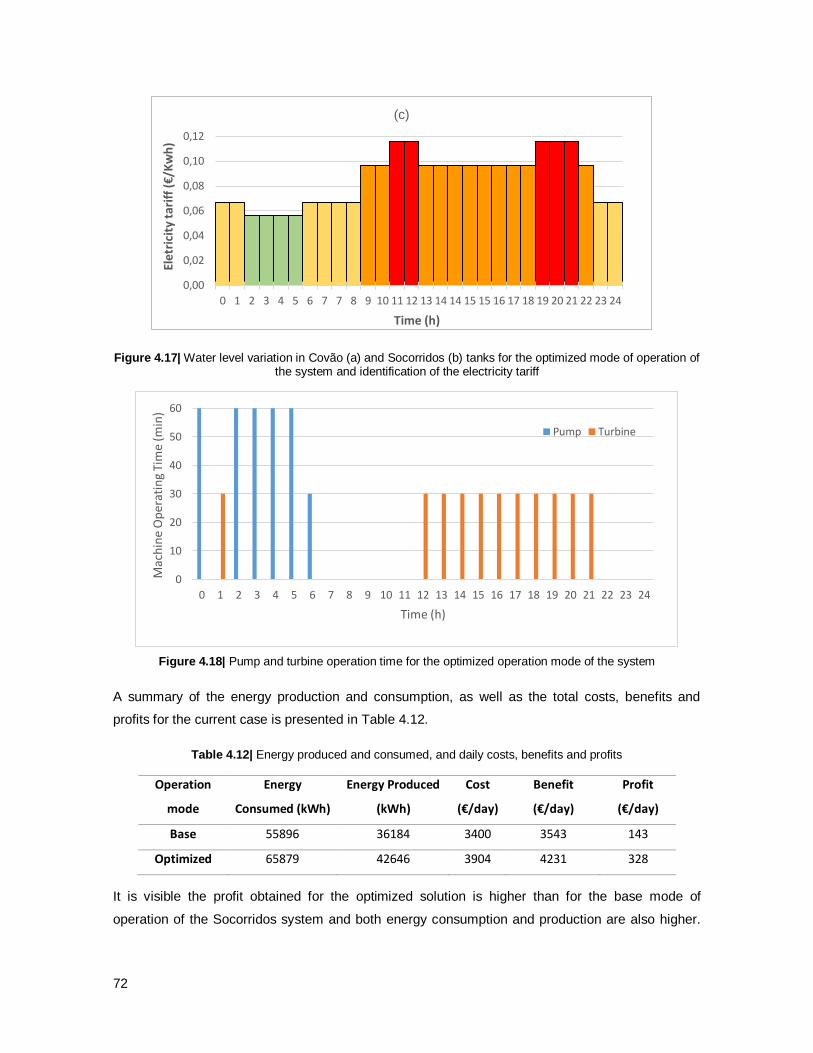
72

Figure 4.17| Water level variation in Covão (a) and Socorridos (b) tanks for the optimized mode of operation of the system and identification of the electricity tariff

Figure 4.18| Pump and turbine operation time for the optimized operation mode of the system

A summary of the energy production and consumption, as well as the total costs, benefits and

profits for the current case is presented in Table 4.12.

Table 4.12| Energy produced and consumed, and daily costs, benefits and profits

Operation

mode

Energy

Consumed (kWh)

Energy Produced

(kWh)

Cost

(€/day)

Benefit

(€/day)

Profit

(€/day)

Base 55896 36184 3400 3543 143

Optimized 65879 42646 3904 4231 328

It is visible the profit obtained for the optimized solution is higher than for the base mode of

operation of the Socorridos system and both energy consumption and production are also higher.

0,00

0,02

0,04

0,06

0,08

0,10

0,12

0 1 2 3 4 5 6 7 7 8 9 10 11 12 13 14 14 15 15 16 17 18 19 20 21 22 23 24

Ele

tric

ity

tari

ff (

€/K

wh

)

Time (h)

(c)

0

10

20

30

40

50

60

0 1 2 3 4 5 6 7 8 9 10 11 12 13 14 15 16 17 18 19 20 21 22 23 24

Mac

hin

e O

per

atin

g Ti

me

(min

)

Time (h)

Pump Turbine

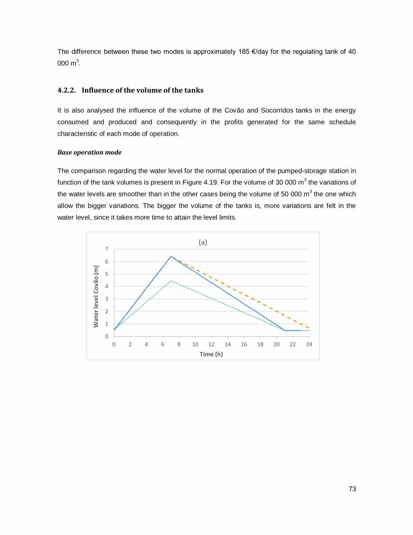
73

The difference between these two modes is approximately 185 €/day for the regulating tank of 40

000 m3.

4.2.2. Influence of the volume of the tanks

It is also analysed the influence of the volume of the Covão and Socorridos tanks in the energy

consumed and produced and consequently in the profits generated for the same schedule

characteristic of each mode of operation.

Base operation mode

The comparison regarding the water level for the normal operation of the pumped-storage station in

function of the tank volumes is present in Figure 4.19. For the volume of 30 000 m3 the variations of

the water levels are smoother than in the other cases being the volume of 50 000 m3 the one which

allow the bigger variations. The bigger the volume of the tanks is, more variations are felt in the

water level, since it takes more time to attain the level limits.

0

1

2

3

4

5

6

7

0 2 4 6 8 10 12 14 16 18 20 22 24

Wat

er le

vel C

ovã

o (m

)

Time (h)

(a)

74

Figure 4.19| Water level variation in Covão (a) and Socorridos (b) tanks for the base operation mode in function of the tanks volume (m

3)

The comparison of the time of operation of the pumps and the turbines for the different volumes is

showed in Figure 4.20. For this mode of operation and independently of the volume, the pump

station only operates during the first six hours of the day while in the remaining time the

hydropower station is working. The time of operation of the pumps in each hour remains constant

and decreases for smaller volumes. Considering the time of operation of the turbines it can be

observed it is the same when the volume of the tanks is 40 000 m3 or 50 000 m

3, but in the first

case the Socorridos tank reaches its maximum at 21 h, then the turbines stop operating. The same

situation happens when the volume is 30 000 m3 but it only operates 10 min in each hour.

0

1

2

3

4

5

0 2 4 6 8 10 12 14 16 18 20 22 24

Wat

er

leve

l So

corr

ido

s (m

)

Time (h)

(b)

50000 30000 40000

0

10

20

30

40

50

60

0 1 2 3 4 5 6 7 8 9 10 11 12 13 14 15 16 17 18 19 20 21 22 23 24

Pu

mp

Op

erat

ion

Tim

e (m

in)

Time (h)

(a)

75

Figure 4.20| Pump (a) and turbine (b) operation time for the base operation mode in function of the tanks volume (m

3)

Optimized operation mode

As showed for the base mode of operation of the system, the comparison regarding the water level

for the optimized mode in function of the tank volumes is present in Figure 4.21. It is observed the

sensitivity in the water level follows the same pattern as in the base operation mode, it is higher for

bigger volumes.

0

5

10

15

20

25

30

0 1 2 3 4 5 6 7 8 9 10 11 12 13 14 15 16 17 18 19 20 21 22 23 24

Turb

ine

Op

era

tio

n T

ime

(m

in)

Time (h)

(b)

50000 40000 30000

0

1

2

3

4

5

6

7

0 2 4 6 8 10 12 14 16 18 20 22 24

Wa

ter

leve

l Co

vão

(m)

Time (h)

(a)

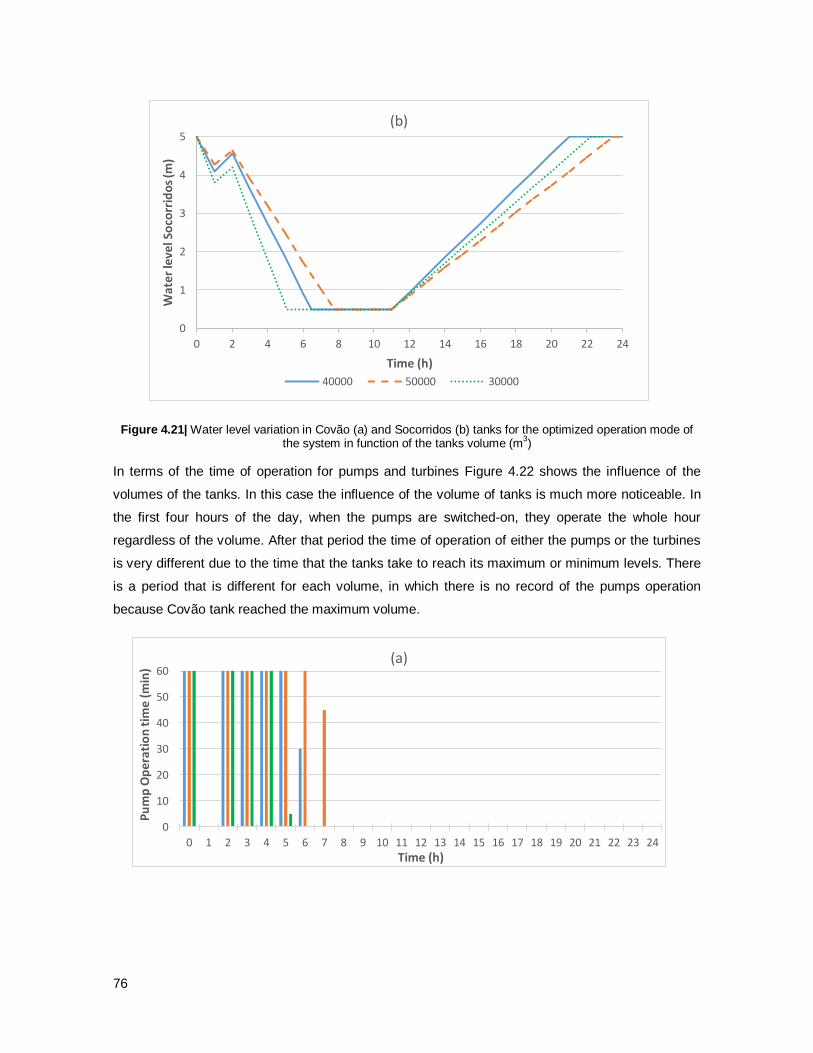
76

Figure 4.21| Water level variation in Covão (a) and Socorridos (b) tanks for the optimized operation mode of the system in function of the tanks volume (m

3)

In terms of the time of operation for pumps and turbines Figure 4.22 shows the influence of the

volumes of the tanks. In this case the influence of the volume of tanks is much more noticeable. In

the first four hours of the day, when the pumps are switched-on, they operate the whole hour

regardless of the volume. After that period the time of operation of either the pumps or the turbines

is very different due to the time that the tanks take to reach its maximum or minimum levels. There

is a period that is different for each volume, in which there is no record of the pumps operation

because Covão tank reached the maximum volume.

0

1

2

3

4

5

0 2 4 6 8 10 12 14 16 18 20 22 24

Wat

er

leve

l So

corr

ido

s (m

)

Time (h)

(b)

40000 50000 30000

0

10

20

30

40

50

60

0 1 2 3 4 5 6 7 8 9 10 11 12 13 14 15 16 17 18 19 20 21 22 23 24

Pu

mp

Op

era

tio

n t

ime

(m

in)

Time (h)

(a)

77

Figure 4.22| Pump (a) and turbine (b) operation time for the optimized mode of operation in function of the tanks volume (m

3)

All the differences of energy consumption/production referred in both modes of operation of the

system and for different volumes of the tanks have influence in terms of profits. An adequate

comparison in terms of energy production, consumption and profits is made and presented in

Table 4.13. The intermediate calculations are presented in Appendix A.3.

Table 4.13| Energy consumed and produced, daily costs, benefits and profits for different tank volumes

Operation mode

Volume of the tank (m3)

Energy Consumed

(kWh)

Energy Produced

(kWh)

Cost (€/day)

Benefit (€/day)

Profit (€/day)

Base

30 000 27948 18092 1700 1771 56

40 000 55896 36184 3400 3543 143

50 000 69870 46523 4250 4437 187

Optimized

30 000 48909 31661 2884 3234 350

40 000 65879 42646 3904 4231 328

50 000 44906 48454 4900 5261 361

Comparing all the results for the base mode of operation, the profit generated is nearly proportional

to the volume of the tank with a lower profit in the case of the smaller tank analysed. The bigger

volume would increase the energy production in 30.8%. The differences of profits become much

more interesting in the analysis of the optimized solution with the smaller volume producing more

energy than the referenced one. In this model the profits generated do not differ much for different

volumes as observed in Figure 4.23.

0

5

10

15

20

25

30

35

0 1 2 3 4 5 6 7 8 9 10 11 12 13 14 15 16 17 18 19 20 21 22 23 24

Turb

ine

op

era

tio

n ti

me

(m

in)

Time (h)

(b)

40000 50000 30000

78

Figure 4.23| Profits generated in the system for the two different modes of programming in function of the volumes of Covão e Socorridos tank

0

50

100

150

200

250

300

350

400

25000 30000 35000 40000 45000 50000 55000

Pro

fit

(€/d

ay)

Resevoirs volume (m3)

Base operation mode Optimized Operation Mode

79

5. CONCLUSIONS

This chapter presents the main conclusions of this document as well as a brief summary of the

review of the results obtained. Following are made some suggestions for future developments of

the work.

Content

5.1. General Conclusions ............................................................................................................. 80

5.2. Further developments............................................................................................................ 81

5

80

5.1. General Conclusions

The present document covers the operating rules and sensitivity analyses towards the best system

efficiencies in two different water supply systems.

The efficient use of energy is critical for the global economic efficiency of utilities. Energy production

and consumption represent a significant part of operating benefits and costs of the water supply

utilities so the theoretical bases of hydropower and pumping station are presented succinctly in this

document. In both case studies the computational simulation based on hydraulic principles

constitutes a powerful tool in the comprehension of the complex effects occurring in each system

characteristics.

In the case study of Beliche several scenarios of turbine operation and energy production are

analysed. It is determined that the best is the one with the turbine running at its maximum efficiency

and only resorting to the second turbine if necessary and with no restrictions concerning efficiencies

and heads values. This scenario produced a total energy in all the 148 days of operation of the

micro-hydro equal to 22.6 MWh which considering an estimation for the whole year would result in

55.8 MWh/year. The same system is also simulated for different types of valves. In the beginning it

is simulated with a TCV in which the parameter of control is the valve headlloss coefficient and in a

second analysis the TCV is replaced by a PRV and a FCV in which the flow is the variable

controlled. In terms of energy produced both designs generated similar values but the constancy of

flow in the turbines in the second case is closer to what was expected in terms of the simulation of

the system. It is also concluded the relation between the energy produced and the mean daily flow

in the Beliche WTP follows a nearly linear regression.

The possibility of installation of the third turbine is also analysed and proved to be viable for both

schemes of sale of the produced energy to the national electric grid or consumption in-situ and for

different initial costs signifying a very important future improvement in the Beliche system. In terms

of remuneration’s schemes, sale of the produced energy would bring slightly bigger benefits than

consumption in-situ.

The same system is also simulated for the case of existing a regulating tank as well as a sensitivity

analysis for key parameters of the models. It is concluded the same system could be simulated and

improved in several ways depending on which type of control and investment required. In the case

of the system controlled by the water level the energy produced increased a lot reaching values of

80 MWh/year. This increment is related to the new capacity of storage of the system allowing the

turbines always operate at their maximum flow until the tank become full.

81

Regarding the volume of the regulating thank it is proved that it would have influence in the energy

produced until volumes near 100 000 m3. For volumes bigger than this the energy produced would

be practically constant.

In the case study of Socorridos is presented the procedure developed in order to improve the

energy and economic efficiency in the pumped-storage system. Optimization routines for the pump

and turbine operation are developed and the best schedule which lead to greater profits are found

for a programming with no hourly operation limitations. The correct utilization of a GA simulator in

an optimization process required running several scenarios, in which is essential to minimize the

model complexity. It can be concluded that the model used is very flexible in terms of input data:

water consumption, tanks volume, maximum flow and electricity tariff.

The results showed that the difference in terms of profit between the base and optimized operation

mode of the pumped-storage system is approximately 185 €/day with the best result for the second

condition with near 320 €/day. This difference represents the diary saving that can be achieved with

the implementation of an optimization in the operation mode of the system when compared to the

current schedule of pump/turbines, maintaining the hydraulic restrictions and water delivery to the

population.

The influence of the volume of the tanks in the profits generated is also analyzed for this case study

concluding that for the base operation mode it increases almost linearly. For the optimized mode of

operation, the profit generated for a tank with 30 000 m3 is quite higher than for the actual case of

40 000 m3 but these value do not differ as much as in the referenced operation mode. In this case

the difference would be of 22 €/day.

5.2. Further developments

Although the study in this thesis has covered a wide range of scenarios and sensitivity analyses of

several parameters there are some more analyses that would be interesting to perform.

Concerning the case study of Beliche it would be relevant in future works to investigate the

following points:

1. Make an economic analysis of the type of valves used;

2. Make an economic analysis of the option of installing a regulating tank;

3. Study the influence of the initial water level of the regulating tank in the behavior of the

system and in the energy produced.

Regarding the case study of Socorridos it is recommended for future works:

1. Study the possibility of the pumps to operate independently of each other at different time;

82

2. Study the possibility of using variable speed drives (VSD) instead of fixed speed drives

(FSD);

3. Determine the best hourly schedule of the system for different volumes of the tanks.

83

6. REFERENCES

[1] Albuquerque, R.B. F., 2006. Projecto de Turbinas Hidráulicas Axiais com Parametrização da

Geometria, Equação de Equilíbrio Radial e Técnicas de Otimização, M.Sc. Thesis, UNIFEI.

[2] Allan, J. F., Nekimken, K. J. And Weills S. B., 2009. Pump Sequencing Optimization. Pump

Efficiency Solutions, California Polytechnic State University.

[3] Amaral, M. 2012, Energy Efficiency and Sustainability - Renewable Energies and Pumped-

Storage M.Sc. Thesis, Instituto Superior Técnico.

[4] Araujo, L.S., Ramos, H., Coelho S.T., 2006. Pressure control for leakage minimization in

water distribution systems management, Water Resources Management, 133 (20), pp.133–149.

[5] Barry, J.A., 2007. WATERGY: Energy and Water Efficiency in Municipal Water Supply and

Wastewater Treatment Cost-Effective Savings of Water and Energy, pp. 1-44.

[6] Carravetta, A., Giudice, G., Fecarotta, O., Ramos, H., 2012. Energy Production in Water

Distribution Networks: A PAT Design Strategy. Water Resour Manage (2012) 26:3947–3959.

[7] Carravetta, A., Giudice, G., Fecarotta, O., Ramos, H., 2013. PAT Design Strategy for Energy

Recovery in Water Distribution Networks by Electrical Regulation. Energies 2013, 6, 411

[8] Carravetta, A., Fecarotta, O., Sinagra, M., Tucciarelli, T., 2012. Turbine Selection For Energy

Production In Water Distribution Networks. Journal of Water Resources Planning and

Management.

[9] Carriço, N., Covas, D., Alegre, H., Almeida, M. 2013. How to Assess the Effectiveness of

Energy Management Processes in Water Supply Systems, In Asset Management for Enhancing

Energy Efficiency in Water and Wastewater Systems, Marbelha.

[10] Casey, M. V.and Keck, H., 1996. Hydraulic turbines. Handbook of Fluid Dynamics and Fluid

Machinery, Eds J. A. Schetzand A. E. Fuhs, John Wiley Inc.

[11] Chapallaz, J.M., Eichenberger, P.,Fischer, G., 1992, Manual on Pumps Used as Turbines,

MHPG Series, Harnessing Water Power on a Small Scale, Volume 11.

[12] Coelho, B., Tavares, A. and Andrade-Campos, A., 2012, Analysis of diverse optimization

algorithms for pump scheduling in water supply systems EngOpt 2012 – 3rd

International

Conference on Engineering Optimization.

[13] Costa, L. H. M., Ramos, H. M. and Castro, M. A. H., 2010. Hybrid genetic algorithm in the

84

optimization of energy costs in water supply networks. Water Science & Technology: Water

Supply—WSTWS Vol 10 No 3 pp 315–326. IWA Publishing. DOI:10.2166/ws.2010.194

[14] Costa, L. H. M., Ramos, H. M. and Castro, M. A. H., 2010. Use of hybrid genetic algorithms

for optimized operation of water supply systems. Eng. Sanit. Ambient. [online]., vol.15, n.2, pp.

187-196. ISSN 1413-4152.

[15] Covas, D. and Ramos, H. 1999. Leakage detection in single pipeline using pressure wave

behavior. Water Industry System: Modelling and optimization application. Baldock, Hertfordshire,

England, pp 287-299.

[16] Covas, D. and Ramos, H. 2010. Case Studies of Leak Detection and Location in Water Pipe

Systems by Inverse Transient Analysis, Journal of Water Resources Planning and Management,

Vol. 136, No. 2, pp. 248-257. DOI: 10.1061/(ASCE)0733-9496(2010)136:2(248).

[17] Darling, D., 2013, The Encyclopedia of Alternative Energy and Sustainable Living.

[18] Deb, K. and Jain, S., 2002. Multi-speed gearbox design using multiobjective evolutionary

algorithms. ASME Transactions on Mechanical. 125(3): 609-619.

[19] Diário da República, 1.ª série — N.º 35 — 19 de fevereiro de 2013.

[20] Diez, P., 2001.Turbinas Hidráulicas, Departamento De Ingenieria Electrica Y Energetica

Universidad De Cantabria.

[21] Direcção-Geral dos recursos naturais, 1991. “Manual de Saneamento Básico”, Volumes 1 e

2 (Ministério do Ambiente e dos Recursos Naturais).

[22] Drtina, P. and Sallaberger, M., 1999. Hydraulic turbines—basic principles and state-of-theart

computational fluid dynamics applications. Proc. Instn. Mech. Engrs, vol. 213 Part C, pp. 85-102.

[23] Engineering Science Data Unit, 2007. Radial, mixed and axial flow pumps, The Institution

mechanical Engineers & The Institution of Chemical Engineers.

[24] Fecarotta, O., Aricó, C., Carravetta, A.,Ramos, H., Martino,R., 2013. Pressure Control And

Hydropower Potential In Water Distribution Networks: Valve Replacement By Pats.

[25] Fecarotta, O., Aricó, C., Carravetta, A.,Ramos, H., Martino,R., 2013. Valve substitution by

PATs.

[26] Filho, L. A. P.: 2006, Um modelo de operação de sistemas adutores de abastecimento de

água com vistas a minimização dos custos energéticos, Universidade Federal de Campina

Grande - Centro de Ciências e Tecnologia.

85

[27] Gonçalves, F. V., Costa, L. H. e Ramos, H.M., 2011. Best economical hybrid energy

solution: Model development and case study of a WDS in Portugal. Energy Policy, v.39, n.6, pp.

3361-3369, 2011.

[28] Khatib, W. and Fleming, P. J., 1997. An Introduction to Evolutionary Computation for

Multidisciplinary Optimisation, Genetic Algorithms in Engineering Systems: Innovations and

Applications.

[29] Konak, A., Coit, D.W., and Smith A.E., 2006. Multi-Objective Optimization Using Genetic

Algorithms: A Tutorial, Reliability Engineering and System Safety, 91, 992-1007.

[30] KSB. 2005. Pumps and Systems. Techno digest.

[31] Lampe, L.K., Adams, L.M., Jensen, D.G., 2009. Water supply and energy generation. Paper

Presented at the World Environmental and Water Resources. pp. 1-10. DOI:

10.1061/41036(342)526.

[32] Lin, M., 2008. The single-row machine layout problem in apparel manufacturing by

hierarchical order-based genetic algorithm, International Journal of Clothing Science and

Technology, Vol. 20 Iss: 5, pp.258 – 270.

[33] Livramento, J. M., 2013. Central micro-hídrica incorporada em adutora, M.Sc. Thesis for

Renewable Energies and Energy Management, Faculdade de Ciências e Tecnologia,

Universidade do Algarve.

[34] Logan, E. Jr., 1993. Turbomachinery: basic theory and applications, Second Edition, CRC

Press. ISBN 13: 9780824715090.

[35] López-Ibáñez, M., Prasad, T. and Paechter, B., 2005. Optimal pump scheduling:

Representation and multiple objectives. Proceedings of the Eighth International Conference on

Computing and Control for the Water Industry (CCWI 2005), volume 1, pages 117–122,

University of Exeter, UK.

[36] Macintyre, A.J. 1980. Bombas e instalações de bombeamento. Editora Guanabara Dois

S.A. Rio de Janeiro, ISBN: 9788521610861.

[37] Massey, B. 2006. Mechanics of fluids. 8th edition. Taylor & Francis, Abingdon.

ISBN 0-415-36205-9.

[38] Michalewicz, Z.,1996, Genetic algorithms + data structures = evolution programs: 3rd ed.

New York: Springer, pp. 387, ISBN 3-540-60676-9.

[39] Miller, R. and Winters, M., 2009. Opportunities for pumped storage: supporting renewable

86

energy goals. Hydro Review, p. 26-38.

[40] Mitchell, M. 1999. An introduction to Genetic Algorithms, Fifth Printing, MIT Press-

Massachusetts Institute of Technology, USA. ISBN 0−262−13316−4.

[41] Moreira, D., Ramos, H., 2012. Energy efficiency in pumping drink-water systems’ operation:

a case study. Journal of Energy, Hindawi Publishing Corporation.

[42] Moreira, D., 2012, Energy cost optimization in a water supply system case study, M.Sc.

Thesis. Instituto Superiro Técnico.

[43] Naldi, G., Artina, A., Bragalli, C., Liserra, T., Marchi, A., 2009. Experimental

investigation of characteristics curves of centrifugal pumps working as turbines, Integrating Water

Systems. p.571-576, LONDON:CRC Press Taylor & Francis Group, ISBN: 9780415548519,

Sheffield (UK).

[44] Nocedal, J. and Wright, S. J., 1999, Numerical Optimization, Springer-Verlag New York.

ISBN 0-387-98793-2.

[45] Obitko, M., 1998, Introduction to Genetic Algorithms. Alemania, University of Applied

Sciences.

[46] Portela, M. M., 2010, Análise da Rentabilidade Económica de PCH. Relatório do CEHIDRO

para o Projecto PCH (Pequenas Centrais Hidroeléctricas), 30 p., Instituto Superior Técnico, IST,

CEHIDRO, Lisboa.

[47] Quintela, A., 2009, Hidráulica, Fundação Calouste Gulbenkian. ISBN 9789723107753

[48] Ramos, H. 2012. Pumped-Storage and Hybrid Energy Solutions Towards the Improvement

of Energy Efficiency in Water Systems, INTECH.

[49] Ramos, H., 1999. Guideline for Design of Small Hydropower Plants. Supported by WREAN

(Western Energy Agency and Network) and DED (Department of Economic Development –

Energy Division), North Ireland and CEHIDRO (Centro de Estudos de Hidrossistemas) DECivil,

IST, Lisbon.

[50] Ramos, H., 2008. Pumped-Storage and Hybrid Energy Solutions Towards the Improvement

of Energy Efficiency in Water Systems. Energy Efficiency – The Innovative Ways for Smart

Energy, the Future Towards Modern Utilities, Chapter 8.

[51] Ramos, H., Mello, M. and De, P., 2010. Clean power in water supply systems as a

sustainable solution: from planning to practical implementation, IWA Publishing,

87

DOI:10.2166/ws.2010.720.

[52] Ramos, H., 2010. Fundamentos e Orientações no Projecto de Aproveitamentos

Hidroeléctricos: critérios e dimensionamento. Texto de apoio à disciplina de Estruturas e

Aproveitamentos Hidráulicos do 5º ano do MEC – IST.

[53] Ramos, H. and Borga, A., 2000. Pump as turbines: an unconventional solution to energy

production. URBWAT, 1(3), 261–265. DOI: 10.1016/S1462-0758(00)00016-9.

[54] Ramos, J. S. and Ramos, H., 2010. Multi-criterion optimization of energy management in

drinking systems, Water Science and Technology: Water Supply, IWA. DOI:10.2166/ws.2010.011

[55] Relatório de Monitorização da Segurança de Abastecimento do Sistema Elétrico Nacional

2013-2030.

[56] Rio Carrillo, A.M., Frei, C., 2009. Water: a key resource in energy production. Energy Policy

37 (11), pp. 4303–4312, DOI: 10.1016/j.enpol.2009.05.074

[57] Samora, I., Ramos, H., Covas, D., Schleiss, A., 2013. Micro-geração no sistema

multimunicipal de água das Águas do Algarve. Central de Beliche. “XII Simposio Iberoamericano

sobre planificación de sistemas de abastecimiento y drenaje”.

[58] Santos, M., 2009. Otimização de Bomba-Turbina Utilizando Programação Quadrática

Sequencial e Algoritmos Genéticos. PhD Thesis, Instituto de Engenharia Mecânica, Universidade

Federal de Itajubá, UNIFEI.

[59] Sarker, R. A. and Newton, C., 2008. Optimization Modeling: A Pratical Introduction, CRC –

Press Taylor & Francis Group, 469p.

[60] Sousa Júnior, F., 2007, Simulação Numérica de Otimização de Projecto de Compressores

Axiais utilizando o Método da Programação Sequencial Quadrática, PhD Thesis, UNIFEI.

[61] Torreira, R. P. 2002. Fluidos térmicos: água, vapor, óleos térmicos. Editora Hemus. ISBN

8528902390.

[62] Tsutiya, M. T., 2001, Redução do custo de energia elétrica em sistemas de abastecimento

de Água, Associação Brasileira de Engenharia Sanitária e Ambiental - ABES.

[63] Tsutiya, M. T., 2004, Abastecimento de Água. 2a edição, Departamento de Engenharia

Hidráulica e Sanitária da USP.

[64] Ulanicki, B., Bounds, P.L.M., Rance, J.P., Reynolds, L., 2000. Open and closed loop

88

pressure control for leakage reduction. Urban Water 2 (2), 105-114. DOI: 10.1016/S1462-

0758(00)00048-0.

[65] Vieira, F. and Ramos, H. 2008. Hybrid solution and pump-storage optimization in water

supply system efficiency: A case study. Elsier, Energy Policy 36:4142-4148.

[66] Vieira, F., Ramos, H. M., Covas, D.I.C. , Almeida, A. B. 2008, Pump-storage optimization

with renewable energy production in water supply systems. International conference on water

and wastewater pumping station design, pp. 99-112.

[67] Vilanova, M., Balestieri, J., Filho, P., 2014, Energy And Hydraulic Efficiency In Conventional

Water Supply Systems. Renewable and Sustainable Energy Reviews, 30, pp. 701-714.

Consulted websites

[68] APREN - Associação de Energias Renováveis (November, 2013). URL:

http://www.apren.pt/;

[69] APREN (November, 2013). URL: http://www.apren.pt/noticias/detalhes.php?id=258.

[70] Direcção-Geral de Energia e Geologia (September 2013).. URL: http://www.dgeg.pt/.

[71] Eco EDP (September, 2013). URL: http://www.eco.edp.pt/pt/.

[72] Eletricidade da Madeira (January, 2014). URL: www.eem.pt.

[73] Estratégia Nacional de Energia (ENE 2020) (September, 2013).

URL: http://www.apren.pt/fotos/editor2/destaques/rcm_29_2010.pdf

[74] James, Adam. Ways to Increase Hydropower Efficiency and Revenues (January, 2014)

URL:http://www.renewableenergyworld.com/rea/news/article/2013/05/three-ways-to-increase-

hydropower-efficiency-and-revenues.

[75] Portal da Energia (October, 2013). URL:http://www.portal-energia.com/rendimento-da-

microgeracao/.

[76] Nally (October 2013). URL: http : //www.mcnallyinstitute.com/index.html.

[77] REN, Redes Energéticas Nacionais, 2011, Informação mensal, sistema electroprodutor

(October 2013). URL: http://www.centrodeinformacao.ren.pt/.

[78] SCENE, Community Energy Specialists (October, 2013). URL:

http://scenetwork.co.uk/node/121.

A-1

A. APPENDICES

Content

A.1. Results obtained in the WaterGEMS model for the Beliche System ...................................... A-2

A.2. 2014 electricity tariff from Madeira Electricity Company ........................................................ A-6

A.3. Calculation of the profit of Socorridos pumped-storage plant ................................................ A-7

A

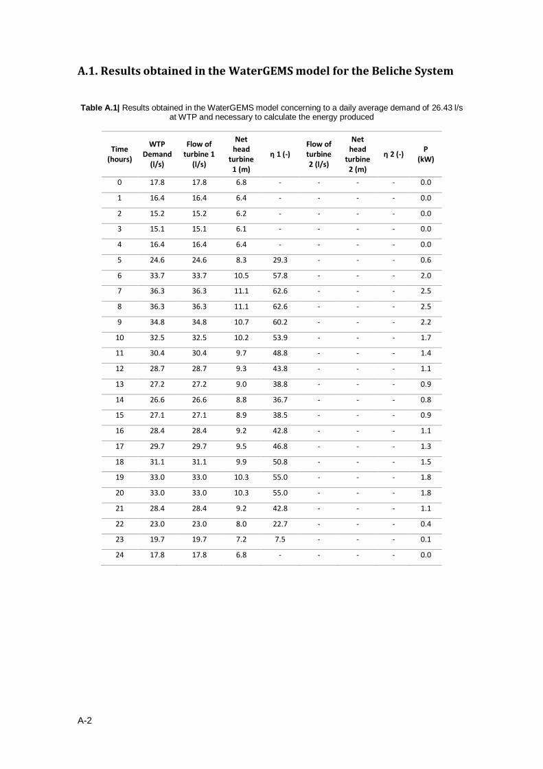
A-2

A.1. Results obtained in the WaterGEMS model for the Beliche System

Table A.1| Results obtained in the WaterGEMS model concerning to a daily average demand of 26.43 l/s at WTP and necessary to calculate the energy produced

Time (hours)

WTP Demand

(l/s)

Flow of turbine 1

(l/s)

Net head

turbine 1 (m)

η 1 (-) Flow of turbine 2 (l/s)

Net head

turbine 2 (m)

η 2 (-) P

(kW)

0 17.8 17.8 6.8 - - - - 0.0

1 16.4 16.4 6.4 - - - - 0.0

2 15.2 15.2 6.2 - - - - 0.0

3 15.1 15.1 6.1 - - - - 0.0

4 16.4 16.4 6.4 - - - - 0.0

5 24.6 24.6 8.3 29.3 - - - 0.6

6 33.7 33.7 10.5 57.8 - - - 2.0

7 36.3 36.3 11.1 62.6 - - - 2.5

8 36.3 36.3 11.1 62.6 - - - 2.5

9 34.8 34.8 10.7 60.2 - - - 2.2

10 32.5 32.5 10.2 53.9 - - - 1.7

11 30.4 30.4 9.7 48.8 - - - 1.4

12 28.7 28.7 9.3 43.8 - - - 1.1

13 27.2 27.2 9.0 38.8 - - - 0.9

14 26.6 26.6 8.8 36.7 - - - 0.8

15 27.1 27.1 8.9 38.5 - - - 0.9

16 28.4 28.4 9.2 42.8 - - - 1.1

17 29.7 29.7 9.5 46.8 - - - 1.3

18 31.1 31.1 9.9 50.8 - - - 1.5

19 33.0 33.0 10.3 55.0 - - - 1.8

20 33.0 33.0 10.3 55.0 - - - 1.8

21 28.4 28.4 9.2 42.8 - - - 1.1

22 23.0 23.0 8.0 22.7 - - - 0.4

23 19.7 19.7 7.2 7.5 - - - 0.1

24 17.8 17.8 6.8 - - - - 0.0

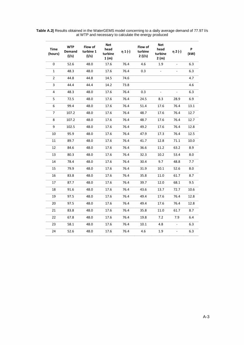
A-3

Table A.2| Results obtained in the WaterGEMS model concerning to a daily average demand of 77.97 l/s at WTP and necessary to calculate the energy produced

Time (hours)

WTP Demand

(l/s)

Flow of turbine 1

(l/s)

Net head

turbine 1 (m)

η 1 (-) Flow of turbine 2 (l/s)

Net head

turbine 2 (m)

η 2 (-) P

(kW)

0 52.6 48.0 17.6 76.4 4.6 1.9 - 6.3

1 48.3 48.0 17.6 76.4 0.3 - - 6.3

2 44.8 44.8 14.5 74.6 4.7

3 44.4 44.4 14.2 73.8 4.6

4 48.3 48.0 17.6 76.4 0.3 - - 6.3

5 72.5 48.0 17.6 76.4 24.5 8.3 28.9 6.9

6 99.4 48.0 17.6 76.4 51.4 17.6 76.4 13.1

7 107.2 48.0 17.6 76.4 48.7 17.6 76.4 12.7

8 107.2 48.0 17.6 76.4 48.7 17.6 76.4 12.7

9 102.5 48.0 17.6 76.4 49.2 17.6 76.4 12.8

10 95.9 48.0 17.6 76.4 47.9 17.3 76.4 12.5

11 89.7 48.0 17.6 76.4 41.7 12.8 71.1 10.0

12 84.6 48.0 17.6 76.4 36.6 11.2 63.2 8.9

13 80.3 48.0 17.6 76.4 32.3 10.2 53.4 8.0

14 78.4 48.0 17.6 76.4 30.4 9.7 48.8 7.7

15 79.9 48.0 17.6 76.4 31.9 10.1 52.6 8.0

16 83.8 48.0 17.6 76.4 35.8 11.0 61.7 8.7

17 87.7 48.0 17.6 76.4 39.7 12.0 68.1 9.5

18 91.6 48.0 17.6 76.4 43.6 13.7 72.7 10.6

19 97.5 48.0 17.6 76.4 49.4 17.6 76.4 12.8

20 97.5 48.0 17.6 76.4 49.4 17.6 76.4 12.8

21 83.8 48.0 17.6 76.4 35.8 11.0 61.7 8.7

22 67.8 48.0 17.6 76.4 19.8 7.2 7.9 6.4

23 58.1 48.0 17.6 76.4 10.1 4.8 - 6.3

24 52.6 48.0 17.6 76.4 4.6 1.9 - 6.3

A-4

Table A.3| Results obtained in the WaterGEMS model concerning to a daily average demand of 95.86 l/s at WTP and necessary to calculate the energy produced

Time (hours)

WTP Demand

(l/s)

Flow of turbine 1

(l/s)

Net head

turbine 1 (m)

η 1 (-) Flow of turbine 2 (l/s)

Net head

turbine 2 (m)

η 2 (-) P

(kW)

0 64.7 48.0 17.6 76.4 16.7 6.5 - 6.3

1 59.4 48.0 17.6 76.4 11.4 5.2 - 6.3

2 55.1 48.0 17.6 76.4 7.1 3.6 - 6.3

3 54.6 48.0 17.6 76.4 6.6 3.3 - 6.3

4 59.4 48.0 17.6 76.4 11.4 5.2 - 6.3

5 89.1 48.0 17.6 76.4 41.1 12.5 70.2 9.9

6 122.2 48.0 17.6 76.4 56.2 17.6 76.4 13.7

7 131.8 48.0 17.6 76.4 49.5 17.6 76.4 12.8

8 131.8 48.0 17.6 76.4 50.9 17.6 76.4 13.0

9 126.1 48.0 17.6 76.4 45.6 15.1 75.6 11.4

10 117.9 48.0 17.6 76.4 46.2 15.6 76.0 11.7

11 110.2 48.0 17.6 76.4 46.6 15.9 76.1 11.9

12 104.0 48.0 17.6 76.4 44.9 14.5 74.8 11.1

13 98.7 48.0 17.6 76.4 46.3 15.7 76.1 11.7

14 96.3 48.0 17.6 76.4 45.6 15.1 75.6 11.4

15 98.3 48.0 17.6 76.4 50.2 17.6 76.4 12.9

16 103.0 48.0 17.6 76.4 50.4 17.6 76.4 13.0

17 107.8 48.0 17.6 76.4 50.6 17.6 76.4 13.0

18 112.6 48.0 17.6 76.4 49.4 17.6 76.4 12.8

19 119.8 48.0 17.6 76.4 54.2 17.6 76.4 13.5

20 119.8 48.0 17.6 76.4 43.9 13.9 72.9 10.7

21 103.0 48.0 17.6 76.4 40.5 12.3 69.3 9.7

22 83.4 48.0 17.6 76.4 35.4 10.9 61.1 8.6

23 71.4 48.0 17.6 76.4 23.4 8.0 24.4 6.8

24 64.7 48.0 17.6 76.4 16.7 6.5 - 6.3

A-5

Table A.4| Results obtained in the WaterGEMS model concerning to a daily average demand of 120 l/s at WTP and necessary to calculate the energy produced

Time (hours)

WTP Demand

(l/s)

Flow of turbine 1

(l/s)

Net head

turbine 1 (m)

η 1 (-) Flow of turbine 2 (l/s)

Net head

turbine 2 (m)

η 2 (-) P

(kW)

0 81.0 48.0 17.6 76.4 33.0 10.3 55.0 8.2

1 74.4 48.0 17.6 76.4 26.4 8.8 36.0 7.1

2 69.0 48.0 17.6 76.4 21.0 7.5 13.8 6.5

3 68.4 48.0 17.6 76.4 20.4 7.3 10.9 6.5

4 74.4 48.0 17.6 76.4 26.4 8.8 36.0 7.1

5 111.6 48.0 17.6 76.4 63.6 17.6 76.4 14.7

6 153.0 48.0 17.6 76.4 47.3 16.6 76.2 12.2

7 165.0 48.0 17.6 76.4 53.9 17.6 76.4 13.4

8 165.0 48.0 17.6 76.4 53.9 17.6 76.4 13.4

9 157.8 48.0 17.6 76.4 49.9 17.6 76.4 12.9

10 147.6 48.0 17.6 76.4 46.4 15.7 76.1 11.8

11 138.0 48.0 17.6 76.4 47.5 16.8 76.3 12.3

12 130.2 48.0 17.6 76.4 48.8 17.6 76.4 12.8

13 123.6 48.0 17.6 76.4 43.6 13.7 72.7 10.6

14 120.6 48.0 17.6 76.4 50.7 17.6 76.4 13.0

15 123.0 48.0 17.6 76.4 54.1 17.6 76.4 13.5

16 129.0 48.0 17.6 76.4 46.9 16.2 76.2 12.0

17 135.0 48.0 17.6 76.4 55.8 17.6 76.4 13.7

18 141.0 48.0 17.6 76.4 49.4 17.6 76.4 12.8

19 150.0 48.0 17.6 76.4 55.0 17.6 76.4 13.6

20 150.0 48.0 17.6 76.4 47.7 17.1 76.3 12.4

21 129.0 48.0 17.6 76.4 42.1 12.9 71.6 10.1

22 104.4 48.0 17.6 76.4 41.8 12.8 71.2 10.1

23 89.4 48.0 17.6 76.4 41.4 12.6 70.6 9.9

24 81.0 48.0 17.6 76.4 33.0 10.3 55.0 8.2

A-6

A.2. 2014 electricity tariff from Madeira Electricity Company

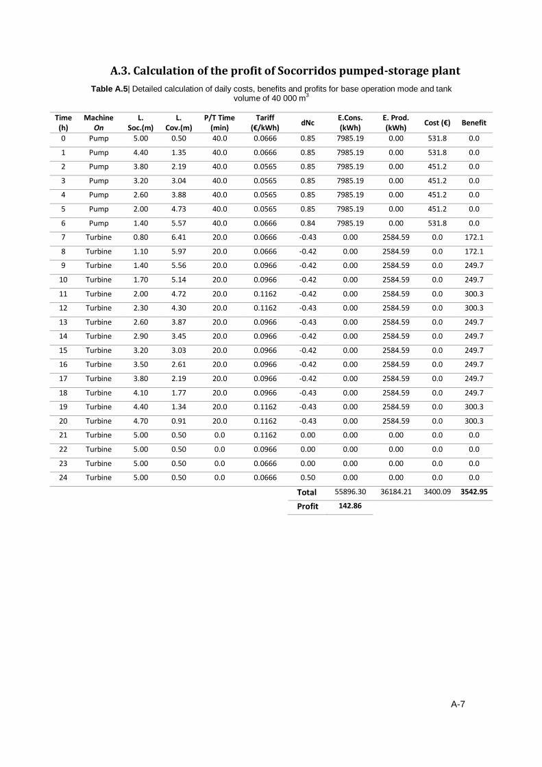
A-7

A.3. Calculation of the profit of Socorridos pumped-storage plant

Table A.5| Detailed calculation of daily costs, benefits and profits for base operation mode and tank volume of 40 000 m

3

Time (h)

Machine On

L. Soc.(m)

L. Cov.(m)

P/T Time (min)

Tariff (€/kWh)

dNc E.Cons. (kWh)

E. Prod. (kWh)

Cost (€) Benefit

0 Pump 5.00 0.50 40.0 0.0666 0.85 7985.19 0.00 531.8 0.0

1 Pump 4.40 1.35 40.0 0.0666 0.85 7985.19 0.00 531.8 0.0

2 Pump 3.80 2.19 40.0 0.0565 0.85 7985.19 0.00 451.2 0.0

3 Pump 3.20 3.04 40.0 0.0565 0.85 7985.19 0.00 451.2 0.0

4 Pump 2.60 3.88 40.0 0.0565 0.85 7985.19 0.00 451.2 0.0

5 Pump 2.00 4.73 40.0 0.0565 0.85 7985.19 0.00 451.2 0.0

6 Pump 1.40 5.57 40.0 0.0666 0.84 7985.19 0.00 531.8 0.0

7 Turbine 0.80 6.41 20.0 0.0666 -0.43 0.00 2584.59 0.0 172.1

8 Turbine 1.10 5.97 20.0 0.0666 -0.42 0.00 2584.59 0.0 172.1

9 Turbine 1.40 5.56 20.0 0.0966 -0.42 0.00 2584.59 0.0 249.7

10 Turbine 1.70 5.14 20.0 0.0966 -0.42 0.00 2584.59 0.0 249.7

11 Turbine 2.00 4.72 20.0 0.1162 -0.42 0.00 2584.59 0.0 300.3

12 Turbine 2.30 4.30 20.0 0.1162 -0.43 0.00 2584.59 0.0 300.3

13 Turbine 2.60 3.87 20.0 0.0966 -0.43 0.00 2584.59 0.0 249.7

14 Turbine 2.90 3.45 20.0 0.0966 -0.42 0.00 2584.59 0.0 249.7

15 Turbine 3.20 3.03 20.0 0.0966 -0.42 0.00 2584.59 0.0 249.7

16 Turbine 3.50 2.61 20.0 0.0966 -0.42 0.00 2584.59 0.0 249.7

17 Turbine 3.80 2.19 20.0 0.0966 -0.42 0.00 2584.59 0.0 249.7

18 Turbine 4.10 1.77 20.0 0.0966 -0.43 0.00 2584.59 0.0 249.7

19 Turbine 4.40 1.34 20.0 0.1162 -0.43 0.00 2584.59 0.0 300.3

20 Turbine 4.70 0.91 20.0 0.1162 -0.43 0.00 2584.59 0.0 300.3

21 Turbine 5.00 0.50 0.0 0.1162 0.00 0.00 0.00 0.0 0.0

22 Turbine 5.00 0.50 0.0 0.0966 0.00 0.00 0.00 0.0 0.0

23 Turbine 5.00 0.50 0.0 0.0666 0.00 0.00 0.00 0.0 0.0

24 Turbine 5.00 0.50 0.0 0.0666 0.50 0.00 0.00 0.0 0.0

Total 55896.30 36184.21 3400.09 3542.95

Profit 142.86

A-8

Table A.6| Detailed calculation of daily costs, benefits and profits for optimized mode of operation and tank volume of 40 000 m

3

Time (h)

Machine On

L. Soc.(m)

L. Cov.(m)

P/T Time (min)

Tariff (€/kWh)

dNc E.Cons. (kWh)

E. Prod. (kWh)

Cost (€) Benefit

0.00 Pump 5.00 0.50 60.0 1.27 0.0666 11977.78 0.00 797.7 0.0

1.00 Turbine 4.10 1.77 30.0 -0.62 0.0666 0.00 3876.88 0.0 258.2

2.00 Pump 4.55 1.14 60.0 1.27 0.0565 11977.78 0.00 676.7 0.0

3.00 Pump 3.65 2.41 60.0 1.27 0.0565 11977.78 0.00 676.7 0.0

4.00 Pump 2.75 3.67 60.0 1.27 0.0565 11977.78 0.00 676.7 0.0

5.00 Pump 1.85 4.94 60.0 1.27 0.0565 11977.78 0.00 676.7 0.0

6.00 Pump 0.95 6.20 60.0 0.63 0.0666 5989.72 0.00 398.9 0.0

6.50 Pump 0.50 6.83 0.0 0.00 0.0666 0.00 0.00 0.0 0.0

7.00 Pump 0.50 6.83 60.0 0.00 0.0666 0.00 0.00 0.0 0.0

8.00 Pump 0.50 6.81 60.0 0.00 0.0666 0.00 0.00 0.0 0.0

9.00 Pump 0.50 6.82 60.0 0.00 0.0966 0.00 0.00 0.0 0.0

10.00 Pump 0.50 6.82 60.0 0.00 0.0966 0.00 0.00 0.0 0.0

11.00 Turbine 0.95 6.19 30.0 -0.63 0.1162 0.00 3876.88 0.0 450.5

12.00 Turbine 1.40 5.56 30.0 -0.64 0.1162 0.00 3876.88 0.0 450.5

13.00 Turbine 1.85 4.92 30.0 -0.64 0.0966 0.00 3876.88 0.0 374.5

14.00 Turbine 2.30 4.29 30.0 -0.63 0.0966 0.00 3876.88 0.0 374.5

15.00 Turbine 2.75 3.66 30.0 -0.63 0.0966 0.00 3876.88 0.0 374.5

16.00 Turbine 3.20 3.03 30.0 -0.63 0.0966 0.00 3876.88 0.0 374.5

17.00 Turbine 3.65 2.40 30.0 -0.63 0.0966 0.00 3876.88 0.0 374.5

18.00 Turbine 4.10 1.77 30.0 -0.64 0.0966 0.00 3876.88 0.0 374.5

19.00 Turbine 4.55 1.13 30.0 -0.64 0.1162 0.00 3876.88 0.0 450.5

20.00 Turbine 5.00 0.50 30.0 0.00 0.1162 0.00 0.54 0.0 0.1

21.00 Turbine 5.00 0.50 0.0 0.00 0.1162 0.00 0.00 0.0 0.0

22.00 Turbine 5.00 0.50 0.0 0.00 0.0966 0.00 0.00 0.0 0.0

23.00 Turbine 5.00 0.50 0.0 0.00 0.0666 0.00 0.00 0.0 0.0

24.00 Turbine 5.00 0.50 0.0 0.00 0.0666 0.00 0.00 0.0 0.0

Total 65878.61 42646.22 3903.61 4231.29

Profit 327.68

A-9

Table A.7| Detailed calculation of daily costs, benefits and profits for optimized mode of operation and tank volume of 30 000 m

3

Time (h)

Machine On

L. Soc.(m)

L. Cov.(m)

P/T Time (min)

Tariff (€/kWh)

dNc E.Cons. (kWh)

E. Prod. (kWh)

Cost (€) Benefit

0.00 pump 5.00 0.50 60.0 0.0666 1.69 11977.78 0.00 797.7 0.0

1.00 turbine 3.80 2.19 20.0 0.0666 -0.55 0.00 2584.59 0.0 172.1

2.00 pump 4.20 1.63 60.0 0.0565 1.69 11977.78 0.00 676.7 0.0

3.00 pump 3.00 3.32 60.0 0.0565 1.69 11977.78 0.00 676.7 0.0

4.00 pump 1.80 5.01 60.0 0.0565 1.69 11977.78 0.00 676.7 0.0

5.00 pump 0.60 6.69 60.0 0.0565 0.14 998.28 0.00 56.4 0.0

5.08 pump 0.50 6.84 0.0 0.0565 0.01 0.00 0.00 0.0 0.0

6.00 pump 0.50 6.84 0.0 0.0666 0.00 0.00 0.00 0.0 0.0

7.00 pump 0.50 6.84 0.0 0.0666 -0.02 0.00 0.00 0.0 0.0

8.00 pump 0.50 6.82 0.0 0.0666 0.00 0.00 0.00 0.0 0.0

9.00 pump 0.50 6.82 0.0 0.0966 0.00 0.00 0.00 0.0 0.0

10.00 pump 0.50 6.82 0.0 0.0966 0.00 0.00 0.00 0.0 0.0

11.00 turbine 0.50 6.82 20.0 0.1162 -0.56 0.00 2584.59 0.0 300.3

12.00 turbine 0.90 6.26 20.0 0.1162 -0.57 0.00 2584.59 0.0 300.3

13.00 turbine 1.30 5.70 20.0 0.0966 -0.57 0.00 2584.59 0.0 249.7

14.00 turbine 1.70 5.13 20.0 0.0966 -0.56 0.00 2584.59 0.0 249.7

15.00 turbine 2.10 4.57 20.0 0.0966 -0.56 0.00 2584.59 0.0 249.7

16.00 turbine 2.50 4.01 20.0 0.0966 -0.56 0.00 2584.59 0.0 249.7

17.00 turbine 2.90 3.45 20.0 0.0966 -0.56 0.00 2584.59 0.0 249.7

18.00 turbine 3.30 2.89 20.0 0.0966 -0.57 0.00 2584.59 0.0 249.7

19.00 turbine 3.70 2.32 20.0 0.1162 -0.57 0.00 2584.59 0.0 300.3

20.00 turbine 4.10 1.75 20.0 0.1162 -0.57 0.00 2584.59 0.0 300.3

21.00 turbine 4.50 1.18 20.0 0.1162 -0.56 0.00 2584.59 0.0 300.3

22.00 turbine 4.90 0.62 20.0 0.0966 -0.14 0.00 646.23 0.0 62.4

22.25 turbine 5.00 0.48 0.0 0.0966 0.00 0.00 0.00 0.0 0.0

23.00 turbine 5.00 0.48 20.0 0.0666 0.00 0.00 0.00 0.0 0.0

23.00 turbine 5.00 0.48 0.0 0.0666 0.00 0.00 0.00 0.0 0.0

24.00 turbine 5.00 0.49 0.0 0.0666 0.00 0.00 0.00 0.0 0.0

Total 48909.39 31661.27 2884.36 3234.23

Profit 349.87

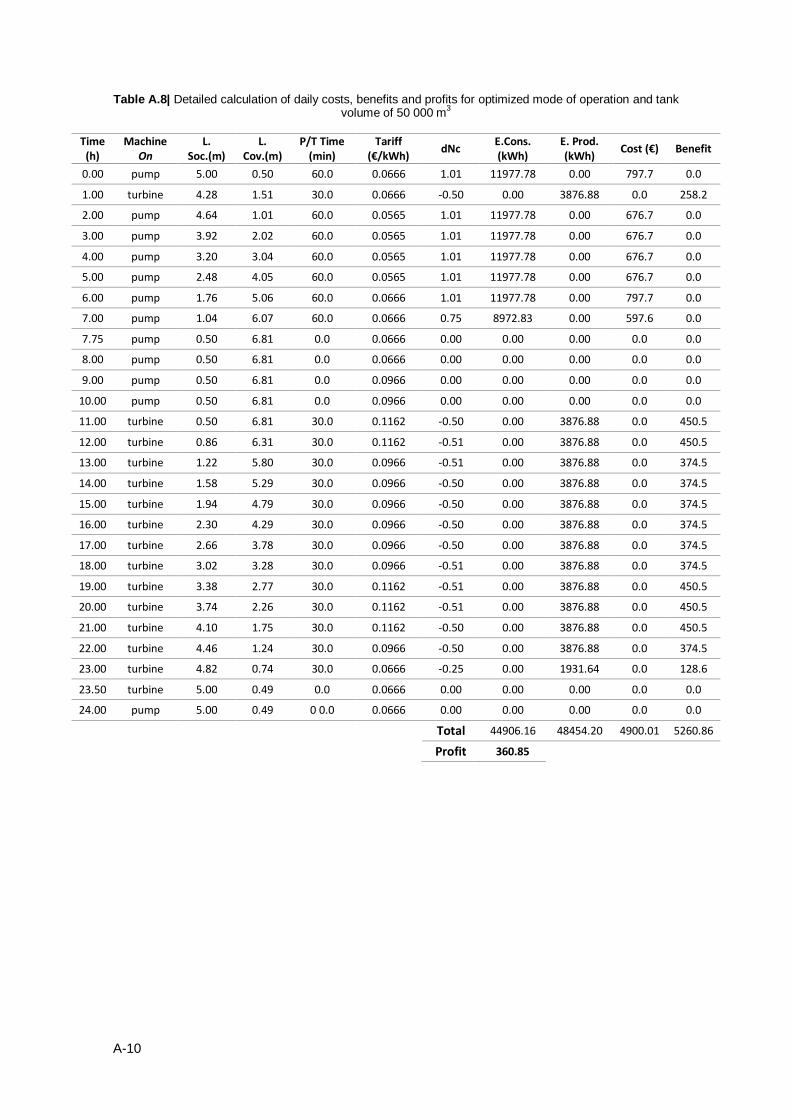
A-10

Table A.8| Detailed calculation of daily costs, benefits and profits for optimized mode of operation and tank volume of 50 000 m

3

Time (h)

Machine On

L. Soc.(m)

L. Cov.(m)

P/T Time (min)

Tariff (€/kWh)

dNc E.Cons. (kWh)

E. Prod. (kWh)

Cost (€) Benefit

0.00 pump 5.00 0.50 60.0 0.0666 1.01 11977.78 0.00 797.7 0.0

1.00 turbine 4.28 1.51 30.0 0.0666 -0.50 0.00 3876.88 0.0 258.2

2.00 pump 4.64 1.01 60.0 0.0565 1.01 11977.78 0.00 676.7 0.0

3.00 pump 3.92 2.02 60.0 0.0565 1.01 11977.78 0.00 676.7 0.0

4.00 pump 3.20 3.04 60.0 0.0565 1.01 11977.78 0.00 676.7 0.0

5.00 pump 2.48 4.05 60.0 0.0565 1.01 11977.78 0.00 676.7 0.0

6.00 pump 1.76 5.06 60.0 0.0666 1.01 11977.78 0.00 797.7 0.0

7.00 pump 1.04 6.07 60.0 0.0666 0.75 8972.83 0.00 597.6 0.0

7.75 pump 0.50 6.81 0.0 0.0666 0.00 0.00 0.00 0.0 0.0

8.00 pump 0.50 6.81 0.0 0.0666 0.00 0.00 0.00 0.0 0.0

9.00 pump 0.50 6.81 0.0 0.0966 0.00 0.00 0.00 0.0 0.0

10.00 pump 0.50 6.81 0.0 0.0966 0.00 0.00 0.00 0.0 0.0

11.00 turbine 0.50 6.81 30.0 0.1162 -0.50 0.00 3876.88 0.0 450.5

12.00 turbine 0.86 6.31 30.0 0.1162 -0.51 0.00 3876.88 0.0 450.5

13.00 turbine 1.22 5.80 30.0 0.0966 -0.51 0.00 3876.88 0.0 374.5

14.00 turbine 1.58 5.29 30.0 0.0966 -0.50 0.00 3876.88 0.0 374.5

15.00 turbine 1.94 4.79 30.0 0.0966 -0.50 0.00 3876.88 0.0 374.5

16.00 turbine 2.30 4.29 30.0 0.0966 -0.50 0.00 3876.88 0.0 374.5

17.00 turbine 2.66 3.78 30.0 0.0966 -0.50 0.00 3876.88 0.0 374.5

18.00 turbine 3.02 3.28 30.0 0.0966 -0.51 0.00 3876.88 0.0 374.5

19.00 turbine 3.38 2.77 30.0 0.1162 -0.51 0.00 3876.88 0.0 450.5

20.00 turbine 3.74 2.26 30.0 0.1162 -0.51 0.00 3876.88 0.0 450.5

21.00 turbine 4.10 1.75 30.0 0.1162 -0.50 0.00 3876.88 0.0 450.5

22.00 turbine 4.46 1.24 30.0 0.0966 -0.50 0.00 3876.88 0.0 374.5

23.00 turbine 4.82 0.74 30.0 0.0666 -0.25 0.00 1931.64 0.0 128.6

23.50 turbine 5.00 0.49 0.0 0.0666 0.00 0.00 0.00 0.0 0.0

24.00 pump 5.00 0.49 0 0.0 0.0666 0.00 0.00 0.00 0.0 0.0

Total 44906.16 48454.20 4900.01 5260.86

Profit 360.85

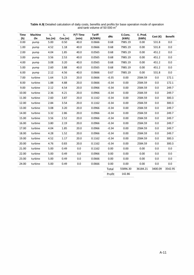
A-11

Table A.9| Detailed calculation of daily costs, benefits and profits for base operation mode of operation and tank volume of 50 000 m

3

Time (h)

Machine On

L. Soc.(m)

L. Cov.(m)

P/T Time (min)

Tariff (€/kWh)

dNc E.Cons. (kWh)

E. Prod. (kWh)

Cost (€) Benefit

0.00 pump 5.00 0.50 40.0 0.0666 0.68 7985.19 0.00 531.8 0.0

1.00 pump 4.52 1.18 40.0 0.0666 0.68 7985.19 0.00 531.8 0.0

2.00 pump 4.04 1.85 40.0 0.0565 0.68 7985.19 0.00 451.2 0.0

3.00 pump 3.56 2.53 40.0 0.0565 0.68 7985.19 0.00 451.2 0.0

4.00 pump 3.08 3.20 40.0 0.0565 0.68 7985.19 0.00 451.2 0.0

5.00 pump 2.60 3.88 40.0 0.0565 0.68 7985.19 0.00 451.2 0.0

6.00 pump 2.12 4.56 40.0 0.0666 0.67 7985.19 0.00 531.8 0.0

7.00 turbine 1.64 5.23 20.0 0.0666 -0.35 0.00 2584.59 0.0 172.1

8.00 turbine 1.88 4.88 20.0 0.0666 -0.34 0.00 2584.59 0.0 172.1

9.00 turbine 2.12 4.54 20.0 0.0966 -0.34 0.00 2584.59 0.0 249.7

10.00 turbine 2.36 4.21 20.0 0.0966 -0.34 0.00 2584.59 0.0 249.7

11.00 turbine 2.60 3.87 20.0 0.1162 -0.34 0.00 2584.59 0.0 300.3

12.00 turbine 2.84 3.54 20.0 0.1162 -0.34 0.00 2584.59 0.0 300.3

13.00 turbine 3.08 3.20 20.0 0.0966 -0.34 0.00 2584.59 0.0 249.7

14.00 turbine 3.32 2.86 20.0 0.0966 -0.34 0.00 2584.59 0.0 249.7

15.00 turbine 3.56 2.52 20.0 0.0966 -0.34 0.00 2584.59 0.0 249.7

16.00 turbine 3.80 2.19 20.0 0.0966 -0.34 0.00 2584.59 0.0 249.7

17.00 turbine 4.04 1.85 20.0 0.0966 -0.34 0.00 2584.59 0.0 249.7

18.00 turbine 4.28 1.52 20.0 0.0966 -0.34 0.00 2584.59 0.0 249.7

19.00 turbine 4.52 1.17 20.0 0.1162 -0.34 0.00 2584.59 0.0 300.3

20.00 turbine 4.76 0.83 20.0 0.1162 -0.34 0.00 2584.59 0.0 300.3

21.00 turbine 5.00 0.49 0.0 0.1162 0.00 0.00 0.00 0.0 0.0

22.00 turbine 5.00 0.49 0.0 0.0966 0.00 0.00 0.00 0.0 0.0

23.00 turbine 5.00 0.49 0.0 0.0666 0.00 0.00 0.00 0.0 0.0

24.00 turbine 5.00 0.49 0.0 0.0666 0.00 0.00 0.00 0.0 0.0

Total 55896.30 36184.21 3400.09 3542.95

Profit 142.86

A-12

Table A.10| Detailed calculation of daily costs, benefits and profits for base mode of operation of the system and tank volume of 30 000 m

3

Time (h)

Machine On

L. Soc.(m)

L. Cov.(m)

P/T Time (min)

Tariff (€/kWh)

dNc E.Cons. (kWh)

E. Prod. (kWh)

Cost (€) Benefit

0.00 pump 5.00 0.50 40.0 0.0666 1.13 7985.19 0.00 531.8 0.0

1.00 pump 4.20 1.63 40.0 0.0666 1.13 7985.19 0.00 531.8 0.0

2.00 pump 3.40 2.75 40.0 0.0565 1.13 7985.19 0.00 451.2 0.0

3.00 pump 2.60 3.88 40.0 0.0565 1.13 7985.19 0.00 451.2 0.0

4.00 pump 1.80 5.01 40.0 0.0565 1.13 7985.19 0.00 451.2 0.0

5.00 pump 1.00 6.13 40.0 0.0565 0.70 4990.87 0.00 282.0 0.0

5.63 pump 0.50 6.84 0.0 0.0565 0.00 0.00 0.00 0.0 0.0

6.00 pump 0.50 6.84 0.0 0.0666 0.00 0.00 0.00 0.0 0.0

7.00 turbine 0.50 6.84 20.0 0.0666 -0.58 0.00 2584.59 0.0 172.1

8.00 turbine 0.90 6.26 20.0 0.0666 -0.56 0.00 2584.59 0.0 172.1

9.00 turbine 1.30 5.70 20.0 0.0966 -0.56 0.00 2584.59 0.0 249.7

10.00 turbine 1.70 5.14 20.0 0.0966 -0.56 0.00 2584.59 0.0 249.7

11.00 turbine 2.10 4.58 20.0 0.1162 -0.56 0.00 2584.59 0.0 300.3

12.00 turbine 2.50 4.02 20.0 0.1162 -0.57 0.00 2584.59 0.0 300.3

13.00 turbine 2.90 3.46 20.0 0.0966 -0.57 0.00 2584.59 0.0 249.7

14.00 turbine 3.30 2.89 20.0 0.0966 -0.56 0.00 2584.59 0.0 249.7

15.00 turbine 3.70 2.33 20.0 0.0966 -0.56 0.00 2584.59 0.0 249.7

16.00 turbine 4.10 1.77 20.0 0.0966 -0.56 0.00 2584.59 0.0 249.7

17.00 turbine 4.50 1.21 20.0 0.0966 -0.56 0.00 2584.59 0.0 249.7

18.00 turbine 4.90 0.65 20.0 0.0966 -0.14 0.00 646.23 0.0 62.4

18.25 turbine 5.00 0.51 0.0 0.0966 -0.01 0.00 0.00 0.0 0.0

19.00 turbine 5.00 0.50 0.0 0.1162 -0.01 0.00 0.00 0.0 0.0

20.00 turbine 5.00 0.49 0.0 0.1162 -0.01 0.00 0.00 0.0 0.0

21.00 turbine 5.00 0.48 0.0 0.1162 0.00 0.00 0.00 0.0 0.0

22.00 turbine 5.00 0.48 0.0 0.0966 0.00 0.00 0.00 0.0 0.0

23.00 turbine 5.00 0.48 0.0 0.0666 0.01 0.00 0.00 0.0 0.0

24.00 turbine 5.00 0.49 0.0 0.0666 0.00 0.00 0.00 0.0 0.0

Total 44916.80 29076.68 2699.10 2755.05

Profit 55.95