Embed Size (px)
Citation preview

Public Infrastructure Investments, Productivity and Welfare in Fixed Geographic Areas
Andrew F. HaughwoutFederal Reserve Bank of New York
AbstractMeasures of the value of public investments are critical inputs into the policy process, andaggregate production and cost functions have become the dominant methods of evaluating thesebenefits. This paper examines the limitations of these approaches in light of applied productionand spatial equilibrium theories. A spatial general equilibrium model of an economy withnontraded, localized public goods like infrastructure is proposed, and a method for identifyingthe role of public capital in firm production and household preferences is derived. Empiricalevidence from a sample of large US cities suggests that while public capital provides significantproductivity and consumption benefits, an ambitious program of locally funded infrastructureprovision would likely generate negative net benefits for these cities.
Keywords: Infrastructure, Regional Economics, Regional Land and Labor Markets
The author is grateful for the comments of two anonymous referees, Roger Gordon, JosephGyourko, Robert Inman, Michael Rothschild, Joseph Tracy and seminar participants at CaseWestern Reserve University, Princeton University and University of Pennsylvania. The viewsexpressed here are the author s, and do not necessarily reflect those of the Federal Reserve Bankof New York or the Federal Reserve System. This work was funded, in part, by financial supportfrom the National Science Foundation and the US and New Jersey Departments ofTransportation subcontract #882090, while the author was at Princeton University. Remainingerrors are my own.

1
I. The debate over infrastructure
While the value of public capital has been a subject of substantial controversy, recent
research has primarily focused on only one component of infrastructure s effect. But the nation s
infrastructure investment has many dimensions. Among these are the consumption value of
public capital, its productivity, and its role in influencing the location of economic activity. This
paper addresses these dimensions simultaneously by providing both a new method and a new
data set for estimating infrastructure benefits.
Public capital may influence social welfare in two ways. The first is through income. If
infrastructure contributes positively to private productivity, then more infrastructure will raise
incomes and increase welfare. Concern about the role of public investment policies in
productivity growth has generated many recent studies attempting to explore the role of
infrastructure in private production, particularly since Aschauer (1989) used national time series
data to estimate an astonishingly high marginal productivity for public capital.
While the marginal productivity of public capital is certainly one component of its
aggregate social value, many of the most prominent authors in the ongoing debate over
infrastructure productivity have recognized that direct, non-pecuniary, household benefits are a
second avenue by which infrastructure may affect welfare. The direct consumption benefits of
public capital have been a less direct focus of current scholarship, even though findings of zero
productivity do not by themselves lead to the conclusion that infrastructure is efficiently
supplied. Instead, reliable results from productivity and household studies must be combined
with cost information to answer the normative question of whether the nation would benefit by
directing more of its resources to public investment. This paper explores the limitations in

2
current approaches to estimating infrastructure s contribution to productivity and provides a new
strategy for analyzing the value of public capital in production and consumption. The alternative
described here provides a fuller and more theoretically consistent accounting of these benefits,
and allows clearer insight into the normative issues involved in infrastructure decision making.
Aschauer s study opened a veritable growth industry in infrastructure research, much of
which utilized the aggregate production, or the analogous aggregate cost function, approaches.
The problems inherent in satisfactory estimation of relationships among short, non-stationary
time series (Aaron 1990, Hulten and Schwab 1991) quickly led researchers to explore the
substantial interregional variation in public capital provision within the US. The interregional
approach offers substantial increases in degrees of freedom and thus an opportunity to exploit
more sophisticated statistical methods. Further, the majority of the nation s non-military public
capital stock is owned by state and local governments (Haughwout and Inman 1996, Holtz-Eakin
1994), and those governments are likely to invest in systems that generate benefits concentrated
within their own borders. State/local analyses implicitly recognize that public investments serve
limited geographic areas, and it is likely that the output responses they induce would be
concentrated within these service areas.
Munnell (1990) and Eberts (1990) applied the aggregate production function (APF)
approach to panels of states and metropolitan areas, respectively. Each found significantly
positive output responses, although the implied output elasticities were far lower than Aschauer s
original estimates. Nonetheless, Munnell s estimated state-level output elasticity of 0.15 was
large enough to provoke continued interest in the possibility of unexploited returns to public
investment. More recent refinements to the aggregate production approach have focused

3
thoroughly on the model s statistical properties. In Holtz-Eakin (1994) and Garcia-Mila, McGuire
and Porter (1996), correction of the estimates for unobserved state-level characteristics reduces
the elasticity of public sector capital to zero, suggesting that the findings of Munnell (1990)
resulted from correlations between infrastructure and unmeasured state traits.
In a parallel set of papers, several authors have applied aggregate cost functions (ACFs)
to data sets similar to those used for analysis of aggregate production functions. In the ACF
approach, the marginal productivity of public capital is measured by calculating its role in
reducing private production costs. This is accomplished by estimating the reductions in aggregate
private input utilization that additional public infrastructure allows. ACF estimates have
generally been more favorable than recent APF results to the argument that there is a positive
role for public capital in production. Berndt and Hansson (1992) report that public capital is a
significant cost-reducing factor in a study of the Swedish economy, while Nadiri and Mamuneas
(1994) find the same for twelve U.S. manufacturing industries at the national level. Finally, in a
paper particularly relevant to the current discussion, Morrison and Schwartz (1996) report that
application of the aggregate cost approach to a panel of American states reveals a significant role
for infrastructure in reducing private production costs, even when unmeasured state factors are
controlled. This result appears to conflict directly with the findings of Holtz-Eakin (1994) and
Garcia-Mila, McGuire and Porter (1996), who argued that after controlling for unmeasured state
effects the marginal productivity of public capital is indistinguishable from zero.
The distinction between the APF and ACF approaches to the estimation of factor
productivities is based on contrasting theories of what may be treated as exogenous to firms
(Friedlander 1990, Berndt 1991). Advocates of aggregate production functions implicitly argue

4
that productive inputs (employment, private capital stock, etc.) are exogenously determined, and
firms make output decisions based on the availability of these factors. Under this hypothesis, the
question of infrastructure productivity becomes whether additions to public capital stocks
increase the output that can be obtained from given input stocks. In practice, this is equivalent to
the assumption that disturbances in output will be uncorrelated with quantities of inputs
available.
ACF authors, however, prefer the assumption that input prices, not quantities, are treated
as exogenous by producers. Morrison and Schwartz (1996) concur with Berndt (1991) in
suggesting that ACF estimates are thus free of endogenous variable bias that plagues production
function estimation, an argument that has a long history in the applied production theory
literature. In this literature, authors have emphasized that while input use is clearly endogenous to
production decisions, input prices will, in a competitive economy, be exogenous to the decisions
of any particular firm.1 The ACF and APF approaches thus embody opposite assumptions about
own-price factor supply elasticities. Perfectly inelastic factor supply schedules (quantities given)
suggest the APF approach, while perfect elasticity (prices given) suggests that ACF is the
1Both Diewert (1974) and McFadden (1978) contain useful surveys and original
contributions. This point was originally made in the context of infrastructure productivityestimation by Friedlander (1990).

5
appropriate theoretical framework.
But application of this logic to the aggregate behavior of regions like the US states raises
new issues. There are two sets of reasons to be concerned about the effects of aggregation. First
is the question of whether the relationships among production aggregates can be interpreted. In a
series of papers, Fisher (1968a, 1968b, 1969) studied the conditions for the existence of
consistent relationships between aggregate and microeconomic functions and variables. His
findings are discouraging to those who wish to analyze these measures. The conditions under
which an aggregate production function exists, for example, are found to be quite restrictive, and
even such variables as aggregate capital and labor stocks and aggregate output will be
meaningful only in very special circumstances. Fisher (1969) acknowledges that contemporary
national time series estimates of such aggregate production functions performed surprisingly
well, generally providing output elasticity estimates for labor and private capital near their shares
in total income. He attributes this success to the fact that relative input stocks and prices had not
changed dramatically over the years for which data were available. But if the reliability of
estimated aggregate relationships depends on the stability of relative factor prices and/or
quantities, then the estimates retrieved from aggregated estimating equations would presumably
become less reliable as this stability breaks down. And the stylized fact that relative input prices
and quantities are stable at the national level over time does not necessarily imply that they will
be consistent over time and regions within the nation. Indeed, there is substantial variation across
the states in both input stocks (see, for example, the data in Morrison and Schwartz 1996 and in
Holtz-Eakin 1992) and prices over the post-WWII period (Carlino and Mills 1996). Aggregate
production function estimates have been especially plagued by implausible estimates of the

6
marginal productivities of private inputs (Berndt and Hansson 1992).
Additional to these problems with the interpretation of aggregate variables and
relationships is a second, related, set of issues. While the hypothesis of price exogeneity may be
appropriate for the analysis of individual competitive firms, it is a far less satisfactory description
of regional behavior. Regions like the US states and ex ante defined metropolitan areas have
complex factor markets in which both the pure price- and quantity-taking assumptions are likely
to fail. Instead, an approach that acknowledges the realities of regional factor markets may be
more appropriate.
Since the geographic areas defined as regions (states or federally-defined metropolitan
areas) are pre-determined, their land area represents a fixed factor with an endogenous price
which varies over space. Meanwhile, private capital supply to small regions is perfectly elastic at
a nationally-determined (exogenous) price, but labor supply is neither perfectly elastic nor
inelastic, and both wages and labor supply are endogenous to regions. The compensating
variations literature pioneered by Rosen (1979) and Roback (1982), and extended by Blomquist,
Berger and Hoehn (1988) shows that when regions are profit and utility takers, the value of
unpriced, nontraded regional traits like climate or infrastructure stock will be fully reflected in
local factor prices. Ultimately, maintained hypotheses about what is exogenous to regions are
crucial, as they determine whether factor prices, quantities, or neither can be treated as exogenous
explanatory variables in regional analysis.
Neither of the dominant methods of analyzing infrastructure productivity controls for the
possibility that regional factor prices reflect part of the value of public capital. But if households
and firms are mobile across regions, then wages and land values will vary in response to

7
infrastructure provision, and the ACF and APF approaches can not adequately estimate the
marginal productivity of public capital, let alone its social value. Exploiting regional data to
answer the nation s infrastructure questions requires an empirical method which utilizes plausibly
exogenous variables to identify the dual roles of public capital in firm production technologies
and household consumption. Spatial equilibrium theory provides such a method. Section II
derives and motivates an alternative measure of infrastructure s social value based on spatial
equilibrium, and comments on its implications for aggregate approaches. Section III provides
estimates of the role of public infrastructure in production and consumption in a set of US cities
and Section IV interprets the results and concludes the paper.
II. Model
Following the compensating variations literature pioneered by Rosen (1979) and Roback
(1982), assume that regions are profit rate and utility takers. Like the maintained hypotheses of
the APF and ACF approaches, this is a polar case, but one which is more consistent with both the
concept of spatial equilibrium and the high degree of mobility exhibited by residential and
business activities in the US.
Workers and firms compete for scarce sites across regions. Individual firms produce a
composite output good using a production technology of the form }m,n,Gx{ = x jjjj , where x
is firm production, G is infrastructure available, n is private employment, m is land used by
firms, and j indexes regions.2 For simplicity, assume that the firm s technology exhibits constant
2The exclusion of private capital has no effect on the regional economic equilibrium, as
long as it is freely mobile and its price is determined in national markets, as is assumed here.

8
returns across the private inputs n and m .3 Local input demands per unit of output (referred to
as )G ,W ,R(n jjj1j and )G ,W ,R(m jjj
1j ) will depend on regional prices for land (R) and labor
(W) and infrastructure stocks. The zero-profit equilibrium condition for a firm in the jth region is
then
3Violation of this assumption complicates the analysis but does not weaken the argument
against the aggregative approach.
where }c{• is the firm s unit cost function and Px is the price of the composite output good
which is determined in national or world markets. The jth region s public capital stock is
$productive# to an individual firm if 0 > mpg = G
xj
j∂∂
, or, equivalently, if 0 < G
c
j∂∂
.
A finding that infrastructure is productive in this sense could be important in
models of economic growth. Aschauer (1989), for example, argues that a decline in relative
infrastructure spending was an important contributor to the US productivity growth slowdown
that began in the 1970s, while Munnell (1990, 1992) endorses this position and suggests that
P = }G,R,Wc{ (1) Xjjj

9
infrastructure differentials help explain interregional productivity variations. But as noted above,
infrastructure s contribution to productivity is only one component of its social value.
The empirical literature has treated infrastructure as a pure national (Aschauer 1989),
state (Holtz-Eakin 1994, Morrison and Schwartz 1996) or regional (Eberts 1990) public good.
The aggregate marginal productivity of infrastructure may then be calculated by summing the
individual productivity benefits across firms, G
x = MPG
jj ∂
∂∑ where the summation is over all
firms in the region. The ideal method of analysis of the aggregate role of infrastructure in
production is thus to collect data on individual firms, calculate the marginal productivity of
infrastructure for each, and aggregate these individual productivities to reflect infrastructure s
nature as a public good. In practice, sufficient data on the behavior of individual firms are
unavailable, and researchers have turned to the analysis of aggregate outcomes. It is crucial to
recognize, however, that the question of infrastructure s productivity is a question about its
effects on the output of individual firms, not on aggregate output. Cross-sectional or panel data
evidence that infrastructure is associated with higher aggregate output at the regional level does
not necessarily mean that increasing infrastructure stocks will raise national output, since the
increase in productivity may be entirely associated with relocations of productive factors from
other regions (Haughwout 1998).
The potential for mobility of productive inputs means that even when the productivity of
public capital is the only question of interest, a model of household behavior is necessary if
aggregate data are to be analyzed. Assume that individual households have well-behaved4 utility
4Twice-differentiable, quasi-concave.

10
functions of the form )G,l,xu( = u jjjj , where x and l are, respectively, the household s
consumption of the composite good and land, and j again indexes locations. Households
maximize utility subject to the constraint that their expenditures equal the wage income they earn
by (inelastically) supplying one unit of labor in the local productive process. In a free-mobility
equilibrium, the level of indirect utility achievable by a household is identical across locations, or
V=)(u j • , where V is the nationally determined equilibrium utility level. Thus, the household
must receive a wage (W j ) that, given local land price Rj and infrastructure stock Gj , enables it
to achieve the utility level which it can attain elsewhere:5
5The household s (constant utility) wage bid function is an expenditure function, as the
notation indicates.
).V,P,G,Re( = W (2) Xjjj

11
Public capital G is directly valuable as a consumption good if and only if 0 > G
u
j∂∂
or,
equivalently, if 0 < G
e
j∂∂
.
Following Roback (1982), firm and household equilibrium conditions (1) and (2) may be
implicitly solved for equilibrium local prices W*j and R*
j :
Since both PX and V are exogenous to any small region, local prices will vary with local
infrastructure stocks, the only unpriced, locationally fixed argument of either household or firm
behavior (Roback 1982).6
6In practice, of course, other non-traded public goods and amenities (like taxes and
climate) will affect local prices. See, inter alia, Roback (1982), Blomquist, Berger and Hoehn(1988), Gyourko and Tracy (1991). The current framework is general in that we can consider Gj avector of non-traded goods. This is the treatment adopted in the empirical analysis below.
);V,G,PR( = R (3) jX*j
).V,G,PW( = W (4) jX*j

12
Aggregate Output, Employment and Land Use
Let x = X j*j ∑ , where the summation is over all firms in the region, represent aggregate
output produced in region j. Under the assumption of constant returns over the private inputs at
the firm level, expressions may be derived for aggregate employment, X)*(n = N *j
1j
*j • , land use
by firms, X)*(m = M *j
1j
*j • and land use by households X* )(n* )(l = N* )(l = L *
j1jj
*jj
*j ••• . For
the land market in region j to clear, its available land area L j must be exhausted by firm and
household demands.7 Thus, L = X ) n* l + m( = L + M j*j
1jj
1j
*j
*j , where, as above,m 1
j and n 1j are
firm demands for land and labor per unit output, l j is demand for land by each household, and
X*j is aggregate output produced in the region. Equilibrium aggregate output produced in region
j is then given by
where n* l + m = L 1jj
1j
1j is the total land area utilized by firms and households in the production
of each unit of output.
7The assumption of fixed area is consistent with the analysis of states and other areas of
fixed geography, like metropolitan areas defined ex ante by the federal government. Of course,the appropriate geographic scale for the analysis infrastructure benefits is a crucial question. It isplausible that infrastructure generates costs and benefits that spill over political jurisdictions
boundaries and that regional definitions are themselves endogenous. Evidence on this point isfound in Boarnet (1997) and Haughwout (1997, 1999).
)G ,W ,R(L
L = ) n*l + m(
L = X (5)j
*j
*j
1j
j
1jj
1j
j*j

13
Comparative Statics
Differentiation of (5) reveals the importance of local price adjustment in determining the effects
of infrastructure on aggregate output
where W
l n +
W
n l +
W
m = k *
j
j1j*
j
1j
j*j
1j
W ∂∂
∂∂
∂∂
,R
l n +
R
n l +
R
m = k *
j
j1j*
j
1j
j*j
1j
R ∂∂
∂∂
∂∂
and
G
l n +
G
n l +
G
m = k
j
j1j
j
1j
jj
1j
G ∂∂
∂∂
∂∂
.
Further, employing Shephard s lemma, it is possible to show that
]G
e n +
G
c[
L
1- =
dG
dR (7)
j
1j
j1jj
*j
∂∂
∂∂
and
]G
c l-
G
em[
L
1 =
dG
dW (8)
jj
j
1j1
jj
*j
∂∂
∂∂
Inspection of (7) and (8) provides insights into the equilibrium effects of public
investment. When infrastructure is valuable to both households and firms, both G
c
j∂∂
andG
e
j∂∂
] k + dG
dRk +
dG
dWk[
L
X- =
dG
dX (6) G
j
*j
Rj
*j
W1j
*j
j
*j

14
are negative. In these circumstances, 0 > dG
dR
j
*j , but equilibrium wages may rise or fall, depending
on which sector (firms or households) benefits more from the investment. If infrastructure is
productive but does not directly affect households, then 0 < G
c
j∂∂
, 0 = G
e
j∂∂
, and both land and
labor price effects are positive.
But the sign of dG
dX
j
*j is indeterminate, even when households are indifferent to
infrastructure and infrastructure plays a positive role in the production functions of every
individual firm.8 A finding that 0 > dG
dX
j
*j is not evidence that infrastructure is productive, i.e., it
does not indicate that 0 < G
c
j∂∂
. The role of market prices in compensating firms and households
for the value of unpriced elements of the environment makes it impossible for analyses of
aggregate output and factor demands to uncover the role of infrastructure in either production and
consumption. Only analysis of local price effects can accomplish this goal. It is to this task that
we now turn, after brief examinations of the aggregate social value of infrastructure and the
identification of its separate impacts on households as producers and consumers.
Willingness to pay for infrastructure and measuring public capital s value to firms and
8 Substitution of (7) and (8) into (6) yields a complex expression for the relationship
between aggregate output and infrastructure provision.There is no regular relationship between aproductive public good and aggregate output. See Haughwout (1998) for more detail anddiscussion.

15
households
In addition to providing a more theoretically consistent empirical model of infrastructure
impacts, the compensating variations method allows both calculation of the aggregate social
value of public capital investments and identification of the two avenues by which it affects
welfare.
Private actors evaluations of infrastructure are expressed as their willingness to pay for
additional infrastructure, ceteris paribus. For individual firms, this is G
c-
j∂∂
(constant-profit cost
savings per unit output), while for households it is G
e-
j∂∂
(constant-utility expenditure savings
per household). Aggregate social value is then equivalent to aggregate willingness to pay9:
9Roback (1982) obtains an identical result, but does not apply it to the analysis of public
decision-making.

16
The question of whether there is $enough# infrastructure is thus whether aggregate willingness to
pay for additional infrastructure equals its aggregate social costs. The efficiency rule is thus to
continue investing in public capital as long as new (net) investment increases jurisdictional land
prices (taxes constant). This rule bears no consistent relationship to the test implicit (and
sometimes explicit) in the APF and ACF literature, which is to invest until aggregate marginal
product equals social marginal tax cost, including excess burden (Morrison and Schwartz 1996).
Indeed, it is clear from (6) that public decisions which attempt to maximize output or
employment will not generally be allocatively efficient, at least from the point of view of the
investing jurisdiction.
In spite of the fact that the sign and size of Gd
dW
j
*j are irrelevant to the efficiency of local
public sector activity, its estimation serves a valuable purpose. With it, we can determine the
incidence of infrastructure benefits across the two sectors. This is crucial, since 0 > dG
dX
j
*j cannot
be interpreted as evidence that public good G is productive. But the compensating variations
method allows identification of the separate effects of infrastructure on firm productivity and
household welfare. Rearrangement of (7) and (8) yields
dGdR
L = dGdR)L + M( =
}dG
dRl -
dG
dW{N- )}
dG
dRm +
dG
dWn( {-X- =
G
eN -
G
c X - = SV
*
0
**j
*j
j
*j
jj
*j*
jj
*j1
jj
*j1
j*j
j
*j
j
*jj ∂
∂∂∂

17
)dG
dRm +
dG
dWn( - =
G
c (9)
j
*j1
jj
*j1
jj∂
∂
and
dG
dRl -
dG
dW =
G
e (10)
j
*j
jj
*j
j∂∂
Under the assumption of free mobility, estimates of dG
dW
j
*j and
dG
dR
j
*j can thus be combined with
land use and employment data to separately identify household and firm willingness to pay for
infrastructure (or other public services) located in a particular geographic area.
III. Data, estimation and evidence on the effects of city infrastructure
Calculation of infrastructure s effects on regional prices requires an empirical design
which can distinguish infrastructure effects from those generated by other produced and non-
produced regional traits. The dependent variables for the estimation are central city house prices
and wages from the American Housing Survey national files micro data, while the principal
independent variables are constructed from US Bureau of the Census Government Finances
publication series. While the data set includes detailed information on houses and their residents
that varies within cities in a given year, the fiscal information in a given year varies only across,
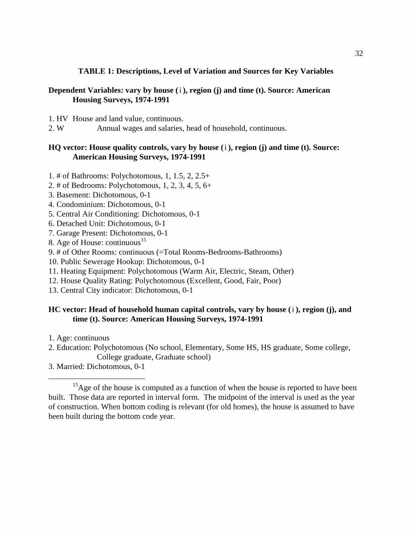
not within, cities. A complete list of variables, the type of variation they provide and their
sources appears in Table 1. Table 2 provides descriptive statistics for the key variables.
The public capital data differ in two key ways from those currently in widespread use.
The replacement value of pubic capital in place is estimated by applying the perpetual inventory
technique to gross-of-depreciation capital investment flows from the early part of this century to

18
the present. Holtz-Eakin (1993) and Munnell (1990) both provide state-level estimates of the
replacement value of public capital in place by apportioning national aggregates to each state
based on the state s share of national gross investment during a benchmark period. This
procedure introduces the possibility of systematic measurement error into the public capital
measure, since investments made during the benchmark period may be correlated with factors
other than historical investment patterns. Because the current method requires no bench marking,
it provides a measure of city and state public capital that is less likely to contain measurement
error.10 Haughwout and Inman (1996) contains a complete description of the public capital data
and 1972-1992 values for each of the central cities analyzed here.
10Garcia-Mila, McGuire and Porter (1996), using an aggregate production function
model, test for and reject the hypothesis that the Munnell series is measured with error.
The infrastructure measure employed here requires data on the investments made by each
government over a long historical period, and such data are available only for state governments
and large cities. While the analysis is thus limited to the effects of infrastructure provision in the
cities listed in Table 3, the addition of sub-state infrastructure variation into the analysis is
valuable. Recent evidence suggests that infrastructure investments have effects on the intra-state
location of economic activities. Boarnet (1997) finds that investments in highway infrastructure
in California counties draw activity from other parts of the state, while Haughwout (1997, 1999)

19
finds that city infrastructure investments increase both city and suburban land values. In
Gyourko, Haughwout and Inman (1997) and Haughwout (1999) state infrastructure investments
are found to reduce city and suburban land values, respectively. Taken together, these results
imply that infrastructure investments have important effects on the intra-state distribution of
activities. If this conclusion is correct, then the case for state-level analysis is considerably
weakened. It also qualifies the interpretation of the empirical analysis performed here. If
infrastructure is found to have a positive marginal benefit in these central cities, it does not
follow that it has positive effects in the state as a whole. Benefits realized in the city jurisdiction
may come at the expense of other areas of the state (as in Boarnet 1996), and/or may spill over to
spatially proximate jurisdictions (Haughwout 1997, 1999).
A two-stage estimation procedure is performed to determine whether city infrastructure
can account for the any of the variance in land prices and wages across metropolitan areas over
time. In the first stage, city-specific effects in land prices and wages over time are computed.
Determining them requires estimation of land price and wage equations:
Here, i , j, and t respectively index individuals, metropolitan areas and time, HV is house value,
W is the household head s wage, and HQ and HC are vectors of house quality and human
capital controls. C j and Tt are, respectively, city and time dummy variables; their interaction
εαα tj,i,tj2tj,i,1tj,i, + T C + HQ = HV (11) •Log
µββ tj,i,tj2tj,i,1tj,i, + T C + HC = W (12) •Log

20
allows estimation of city-year specific effects in house prices and wages. ε tj,i, and µ tj,i, are
standard $white noise# residual terms. These first-stage regressions are estimated with ordinary
least squares over 37,503 households in 33 central cities in 12 cross sections. A list of the cities,
the years they are present in the data set and their mean values for α̂ 2 and β̂ 2 are provided in
Table 3.
The second stage of the estimation strategy involves examining whether variance in local
amenities (Aj ), local or state current tax/service conditions (LTS tj, and STStj,
), and public
infrastructure conditions (LG tj, and SG tj,
) can account for the variance in the estimated city-
specific effects over time in local prices. The α̂ 2 and β̂ 2 vectors (each a 355x1 column vector)
from equations (11) and (12) are then regressed on the city-specific variables:
The coefficients α7 andβ7 retrieved from simultaneous equations estimation of these structural
equations are the estimated land price and wage effects of central city infrastructure stocks,
which are the basis of the willingness to pay calculations provided below.
City land area and city infrastructure specification
Two further estimation issues arise. First, standard urban economic models emphasize the
νβααααααα tj,tj,2,9tj,8tj,7tj,6tj,5j4tj,2, + + SG + LG + STS + LTS + A = (13) ˆˆ
ηαβββββββ tj,tj,2,9tj,8tj,7tj,6tj,5j4tj,2, + + SG + LG + STS + LTS + A = (14) ˆˆ

21
importance of proximity to employment nodes in determining the market value of land, with
centrally located properties commanding the highest locational premia (Fujita, 1989). In the
present context, it is thus likely that physical size of the central city will have a ceteris paribus
effect on the city-specific land price effect, since the sample of houses drawn from a
geographically larger city will be more heavily weighted toward units that are relatively distant
from the central business district. Addition of city land area to the second stage regressions
controls for this element of the AHS sampling design.
A more substantive question that has received little attention in aggregate models is the
congestibility of physical infrastructure. In the majority of recent APF and ACF studies,
infrastructure is measured as the replacement value of the current stock and is treated as a pure,
uncongestible public good. Of course, the true value of infrastructure is the services it provides,
and these services may be (inversely) related to the population utilizing the facility. Here, we
perform a grid search for the proper specification by substituting
POP
STOCK = )STOCKf( = LG
tj,
tj,tj,tj, γ , where γ ranges from 0 (a pure public good specification) to
1 (pure private good).
The grid search reveals that the effect of infrastructure on city land premia falls
monotonically as γ rises. Measured as a pure private good (1 = γ ), infrastructure has an
insignificantly negative effect on land values (and, as is the case for all other values of γ , no
significant effect on wages). As γ falls, the infrastructure coefficient becomes significantly
positive. These effects are driven by the presence of city population in the denominators of the
infrastructure measures. When city population is included as a separate regressor, its coefficient

22
estimate is strongly positive and statistically significant and the coefficient on infrastructure stock
per capita (i.e., 1 = γ ) becomes positive and significant. Under the compensating variations
framework, city populations (like city employment) are endogenous, responding to city land and
labor market conditions rather than the converse. These considerations, along with the fact that
the specification with 0 = γ describes the data best (i.e., it has the lowest mean squared error),
confirm the treatment of infrastructure as uncongestible. This may seem surprising until it is
recognized that the majority of the central cities in the sample have lost population since the
1960s. This suggests the potential for excess capacity in city infrastructure stocks, indicating that
aggregate returns to new investments may be low, a judgement that is supported by the analysis
below.
Effects of city public capital on regional factor prices
Table 4 reports the estimated city infrastructure elasticities retrieved from estimation of
various specifications of equations (13) and (14). The specifications are distinguished by the
assumptions about the linearity of infrastructure s effects on factor prices and by the treatment of
the residual terms ν tj, and η tj, . Specifications 1 and 2 are estimated by three-stage least squares
in order to control for simultaneity in local prices.11 Identification is achieved by omitting city
land area from the wage equation and city crime rates from the land price relationship. The latter
restriction is supported by evidence that crime is perceived as a neighborhood phenomenon.12 In
11The estimated city-year effects in wages and land prices are significantly positively
correlated (r = 0.27).
12 In post-1985 American Housing Surveys, question 50(a) reads: "How would you rate

23
these estimates, infrastructure has a significantly positive effect on city land prices, but wage
effects are indistinguishable from zero.
the neighborhood on a scale of 1 to 10? 10 is best, 1 is worst." Question 50(b) asks for theneighborhood's specific problems to be described, including problems with crime, traffic, andcity or county public services. In Gyourko, Haughwout and Inman (1997), the authors find thatremoving neighborhood quality controls from the first stage regression results in a significantlynegative coefficient on the crime variable in the second stage land price equation, which supportsthis hypothesis. Other identification restrictions do not significantly alter the results presentedhere.
In specifications 3 and 4 of Table 4, controls for simultaneity in prices are replaced with a
two-way variance components estimator (feasible generalized least squares) for city land price
premia. The specification test provided by Hausman (1978) provides little evidence of
misspecification in the variance components estimator, in contrast to similar tests conducted on
the aggregate state production function specification (Garcia-Mila et al, 1996). In these results,
the estimated effect of city infrastructure on land prices is somewhat less precise. Without the
wage equation, the estimates identify only the aggregate social value of infrastructure, but not its

24
components.
Recall from the spatial equilibrium theory described above that were infrastructure a
purely productive input, we would anticipate positive land price and wage effects. Here, the
evidence is that infrastructure provides benefits to both the firm and household sectors. It is also
apparent that the dominant aggregative approaches to infrastructure benefits abstract from
potentially informative covariation between infrastructure provision and local relative prices. The
importance of these relationships emphasizes the role of nontraded public capital investments in
affecting not only the level, but also the spatial distribution of productive and residential
activities.
Results for other second stage variables13
13Details available upon request.
Other second stage variables perform largely as expected. Our climatological and
locational amenity measures are statistically significant and of the expected sign. As anticipated,
the coefficient estimate on land area is negative and significant in the land price equation and
insignificant in the wage equation. Local taxes are negatively capitalized into land prices at rates
near 100%.
The effects of state policy measures are instructive. In spite of the attention paid to
interregional mobility, intrastate migration dominates American residential relocations. During

25
the 1980's and early 1990's, between 80 and 90 percent of residential relocations were within the
same state. What this suggests for the current model is that local and state fiscal policies may
well have substantially different effects. For example, while high city taxes may reduce the
attractiveness of a city location, high state taxes may not, particularly if an active state
government finances some services that other cities must fund from their own tax bases. In such
cases, higher state taxes will lead to higher city land values, as we consistently find here. State
infrastructure stocks have little effect on city land values or wages, as would be expected given
that central cities are relatively small proportions of the states total area. These findings
underline the importance of careful attention to locational decision making in evaluating the
effects of state and local fiscal policies. Models which combine the state and local sectors into
single measures abstract from informative intra-state movements that they differentially induce.
Estimated willingness to pay for central city infrastructure
Producers willingness to pay (WTP) for city infrastructure per unit output is calculated
from equation (9) as )dG
dRm +
dG
dWn( - =
G
c
j
*j1
jj
*j1
jj∂
∂, while for a typical household, WTP is
dG
dRl -
dG
dW =
G
e
j
*j
jj
*j
j∂∂
. The central city benefit generated by a one standard deviation (4.64 billion
constant dollars) increase in mean city infrastructure stock is estimated as dGdR
L*
0 .
Estimates of household and firm willingness to pay for infrastructure are presented in the

26
second panel of Table 4.14 Note that without the wage equation, the components of
infrastructure s social value and its productivity are unidentified. While city infrastructure
provision provides benefits at the margin, the social value of a one standard deviation increase in
city infrastructure is not, for the typical city, sufficient to offset its cost. The largest aggregate
value estimate (line 2 of Table 4) is just over 75% of the $4.64 billion cost required to raise
infrastructure stock in the typical city by a sample standard deviation. It is also apparent that
estimated household infrastructure benefits are substantial, probably exceeding firm benefits.
Finally, the marginal productivity of infrastructure is estimated to be non-negative, but small.
IV. Conclusions
The model and empirical evidence presented here emphasize the importance of
infrastructure investments in affecting the relative attractiveness of places, potentially redirecting
growth from infrastructure-poor areas to those which have invested more heavily. While
investments on the public agenda have evolved from canals and ports aimed at capturing the
trade of unfinished agricultural products to fiber optic cable for providing internet bandwidth,
part of the motivation for such investments has been the idea that they might provide some
locations a competitive advantage vis a vis others (Pred 1966, Markoff 1997). But the
implications of spatial competition among regions has not played a large role in dominant
14These estimates use data from the State of the Nation s Cities data base (Center for
Urban Policy Research, 1996).

27
approaches to modeling infrastructure impacts.
The spatial equilibrium approach adopted here emphasizes the importance of
infrastructure in altering the distribution of economic activity across regions, and re-establishes
the household sector to its joint roles as consumer of infrastructure services, supplier of labor and
competitor in the land market. The model and empirical evidence suggest that central city land
prices are, ceteris paribus, positively associated with infrastructure provision and that the benefits
of a large public capital stock are likely enjoyed by both firms and households. A negative,
statistically significant, firm cost elasticity of infrastructure is estimated. Nonetheless, substantial
increases in city public infrastructure provision are unlikely to provide social benefits sufficient
to offset their costs. On the other hand, it is likely that some of the benefits of city infrastructure
investments spill over into neighboring suburban jurisdictions, suggesting that the estimates
presented here may be a lower bound of the total value of such spending. In addition, from the
point of view of the central city, it is quite likely that generous capital aid from other
governments might make substantial capital investments worth their local cost (see Haughwout
1999 for a discussion).
This last observation points to a weakness of this paper and most of the current literature
on public infrastructure impacts. While the empirical model assumes that infrastructure is
exogenously determined, this is clearly not the case. Indeed, the current approach, in which
infrastructure is envisioned as a contributor to local property values, underlines the complex
relationship between the value of the local tax base and the level of infrastructure investment. It
is clear that a more careful analysis of the determinants of public investment is indicated.
Modeling public investment is complicated by the fact that public capital is only one, albeit

28
generally the largest, component of a portfolio of public assets and liabilities (Haughwout and
Inman 1996). The net local benefit generated by a program of long term borrowing to fund
infrastructure investment is the crucial question faced by local decision makers and the municipal
bond market (for preliminary evidence on this point, see Gyourko, Haughwout and Inman 1997).
Until such a model is developed, however, it is crucial to develop methods of examining the
impact of infrastructure on local areas that are based on a consistent theoretical underpinning. As
demonstrated here, local price effects of public investments must play a prominent role in this
effort.

29
REFERENCES
Aaron, H. 1990. "Discussion of `Why is Infrastructure Important?'" in A. Munnell, ed. Is There a Shortfall in Public Capital Investment?.
Aschauer, D. 1989. "Is Public Expenditure Productive?" Journal of Monetary Economics, Vol. 23, pp. 177-200.
Berndt, E. 1991. The Practice of Econometrics: Classic and Contemporary, Reading, Mass:Addison-Wesley.
Berndt, E. and B. Hannsson. 1991. "Measuring the Contribution of Public Infrastructure Capital in Sweden," Working Paper No. 3842, National Bureau of Economic Research.
Blomquist, G., M. Berger, and J. Hoehn. 1988. "New Estimates of Quality of Life in UrbanAreas," American Economic Review, Vol. 78, pp. 89-107.
Boarnet, M. 1997. $Spillovers and the Locational Effect of Public Infrastructure,# mimeo, School of Social Ecology, University of California, Irvine.
Brueckner, J. 1979. "Property Values, Local Public Expenditure and Economic Efficiency," Journal of Public Economics, Vol. 11, pp. 223-245.
. 1982. "A Test for Allocative Efficiency in the Local Public Sector," Journal of Public Economics, Vol. 19, pp. 311-331.
. 1983. "Property Value Maximization and Public Sector Efficiency," Journal of Urban Economics, Vol. 14, pp. 1-15.
Center for Urban Policy Research, 1996. $State of the Nation s Cities,# New Brunswick, NJ: Rutgers University.
Eberts, R. 1990. "Cross-Sectional Analysis of Public Infrastructure and Regional Productivity Growth," Working Paper No. 9004, Federal Reserve Bank of Cleveland.
Fisher, F. 1968a. $Embodied Technology and the Existence of Labour and OutputAggregates,# Review of Economic Studies, Vol. 35, pp. 391-412.
. 1968b. $Embodied Technology and the Aggregation of Fixed and Movable Capital Goods,# Review of Economic Studies, Vol. 35, pp. 417-428.
. 1969. $The Existence of Aggregate Production Functions,# Econometrica, Vol. 37, No. 4, pp. 553-577.

30
Friedlander, A. 1990. Discussion of !Infrastructure and Regional Economic Performance, in Is There a Shortfall in Public Capital Investment? (A. Munnell, Ed.) Federal ReserveBank of Boston.
Garcia-Mila, T., T. McGuire and R. Porter. 1996. "The Effect of Public Capital in State-Level Production Functions Reconsidered," Review of Economics and Statistics,Vol. 78, pp. 177-180.
Gyourko, J., A. Haughwout and R. Inman. 1997. $State and Local Fiscal Conditions, Public Wealth and Local Land Values,# mimeo, Wharton Real Estate Center, University ofPennsylvania.
Gyourko, J. and J. Tracy. 1991. "The Structure of Local Public Finance and the Quality of Life," Journal of Political Economy, Vol. 99, pp. 774-806.
Haughwout, A. 1997. $Central City Infrastructure Investment and Suburban House Values,#
Regional Science and Urban Economics, Vol. 27, No.1.
. 1998. "Aggregate production functions, interregional equilibrium, and themeasurement of infrastructure productivity," Journal of Urban Economics, Vol. 44, pp. 216-227.
. 1999. $Regional Fiscal Cooperation in Metropolitan Areas: An Exploration,#
Journal of Policy Analysis and Management, Vol. 18, No. 4, pp. 579-600.
Haughwout, A. and R. Inman. 1996. $State and Local Assets and Liabilities, 1972-1992,#
mimeo, Woodrow Wilson School, Princeton University.
Hausman, J. 1978. $Specification Tests in Econometrics,# Econometrica, Vol. 46, pp. 1251-1271.
Holtz-Eakin, D. 1994. "Public-Sector Capital and the Productivity Puzzle," Review ofEconomics and Statistics, Vol. 76, pp. 12-21.
Hulten, C. and R. Schwab. 1991. "Is there too little Public Capital?" presented at conference Infrastructure Needs and Policy Options for the 1990s, American Enterprise Institute.
Markoff, J. 1997. $Old Man Bandwidth: Will Commerce Flourish Where Rivers of Wires Converge?# New York Times, 12/8/97, page D1.
Morrison, C. and A. Schwartz. 1996. "State Infrastructure and Productive Performance," American Economic Review, Vol. 86, no. 5, pp. 1095-1111.

31
Munnell, A., ed. 1990. Is There a Shortfall in Public Capital Investment? Proceedings of a Federal Reserve Bank of Boston Conference held in June 1990.
. 1990. $How Does Infrastructure Affect Regional Economic Performance?# in A.Munnell, ed. Is There a Shortfall in Public Capital Investment?.
. 1992. $Policy Watch: Infrastructure Investment and Economic Growth,# Journal of Economic Perspectives, Vol. 6, No. 4, pp. 189-198.
Pred, A. 1966. The Spatial Dynamics of US Urban-Industrial Growth, 1800-1914, Cambridge: MIT Press.
Roback, J. 1982. "Wages, Rents, and the Quality of Life," Journal of Political Economy, Vol. 90, pp. 1257-1278.
Rosen, S. 1979. $Wage-Based Indexes and the Quality of Life,# in P. Mieszkowski and M. Straszheim, eds., Current Issues in Urban Economics, Baltimore: Johns Hopkins Press.
Wildasin, D. 1986. Urban Public Finance, New York: Harwood.
32
TABLE 1: Descriptions, Level of Variation and Sources for Key Variables
Dependent Variables: vary by house (i ), region (j) and time (t). Source: American Housing Surveys, 1974-1991
1. HV House and land value, continuous.2. W Annual wages and salaries, head of household, continuous.
HQ vector: House quality controls, vary by house (i ), region (j) and time (t). Source: American Housing Surveys, 1974-1991
1. # of Bathrooms: Polychotomous, 1, 1.5, 2, 2.5+2. # of Bedrooms: Polychotomous, 1, 2, 3, 4, 5, 6+3. Basement: Dichotomous, 0-14. Condominium: Dichotomous, 0-15. Central Air Conditioning: Dichotomous, 0-16. Detached Unit: Dichotomous, 0-17. Garage Present: Dichotomous, 0-18. Age of House: continuous15
9. # of Other Rooms: continuous (=Total Rooms-Bedrooms-Bathrooms)10. Public Sewerage Hookup: Dichotomous, 0-111. Heating Equipment: Polychotomous (Warm Air, Electric, Steam, Other)12. House Quality Rating: Polychotomous (Excellent, Good, Fair, Poor)13. Central City indicator: Dichotomous, 0-1
HC vector: Head of household human capital controls, vary by house (i ), region (j), and time (t). Source: American Housing Surveys, 1974-1991
1. Age: continuous2. Education: Polychotomous (No school, Elementary, Some HS, HS graduate, Some college,
College graduate, Graduate school)3. Married: Dichotomous, 0-1
15Age of the house is computed as a function of when the house is reported to have been
built. Those data are reported in interval form. The midpoint of the interval is used as the yearof construction. When bottom coding is relevant (for old homes), the house is assumed to havebeen built during the bottom code year.

33
4. White: Dichotomous, 0-15. Hispanic: Dichotomous, 0-1

34
Table 1, continued
STS and LTS: Local and State Tax and Service vectors, vary by region (j) and year (t).Sources: Government Finances (GF) series (Census a, various years); Significant Featuresof Fiscal Federalism (ACIR, various years); American Housing Survey (AHS), 1974-1991;Digest of Educational Statistics (DES), (Department of Education, various years); UniformCrime Reports (UCR), (FBI, various years).
1. Mean city effective property tax rate: Continuous, Source: AHS2. City income tax rate: Continuous, ACIR3. City sales tax rate: Continuous, ACIR4. Serious crimes per 100,000 population: Continuous, UCR5. Pupil-teacher ratio in city schools: Continuous, DES6. State income tax rate: Continuous, ACIR7. State sales tax rate: Continuous, ACIR8. City infrastructure stock: Continuous, GF and author s calculations (See Haughwout and Inman 1996 for details)9. State infrastructure stock: Continuous, GF and author s calculations (See Haughwout and Inman 1996 for details)
A: Unproduced Amenities, vary by region (j). Source: US Bureau of the Census, City andCounty Data Book, 1987 and author s calculations.
1. Coastal status: Dichotomous, 0-1, author s calculations2. Mean annual rainfall: Continuous3. Mean annual heating degree days: Continuous4. Mean cooling degree days: Continuous

35
TABLE 2: Descriptive Statistics for Second Stage Variables
Variable Mean Std. dev. Min Max
α 2 (Land price effect) 10.39 0.37 9.43 11.79
β 2 (Labor price effect) 7.25 0.20 6.12 7.98
Violent crime (per 100,000 pop) 1,268.95 596.31 385.15 4,041.08
Pupil-teacher ratio 20.12 2.63 12.60 27.40
Property tax rate (%) 1.33 0.66 0.21 3.51
State income tax rate (%) 5.33 3.94 0.00 16.00
State sales tax rate (%) 4.30 1.17 0.00 6.50
Local sales tax rate (%) 1.15 1.09 0.00 5.00
Coastal dummy 0.27 0.44 0.00 1.00
Mean rainfall (inches per yr) 34.37 11.74 7.66 61.88
Heating degree days 4,400.25 2,040.39 137.00 7,981.00
Cooling degree days 1,294.69 947.09 65.00 4,162.00
State infrastructure stock (billionsof $1990)
40.68 23.17 8.19 89.36
City infrastructure stock (billions of$1990)
6.29 4.64 1.77 23.42
City infrastructure stock per capita(thousands of $1990)
8.67 3.45 1.86 19.80
City infrastructure stock, naturallog of $1990 billion
1.65 0.58 0.57 3.15
City Land area (sq mi) 192.3 153.8 40.6 666.2
City population 813,936 683,041 331,163 3,487,390

36
TABLE 3: Estimated City Land Price and Wage Effects
Mean Mean City Years of data* α̂ 2 β 2
1 Atlanta 10.39 7.08 2 Baltimore 10.36 7.27 3 Boston 74-79, 83-91 10.71 7.24 4 Buffalo 74-83 9.90 7.06 5 Chicago 10.47 7.29 6 Cincinnati 10.25 7.27 7 Cleveland 10.08 7.26 8 Columbus 10.22 7.31 9 Dallas 10.38 7.33 10 Denver 10.61 7.17 11 Detroit 9.91 7.36 12 Ft. Worth 10.16 7.27 13 Houston 10.36 7.27 14 Indianapolis 10.15 7.26 15 Kansas City, Missouri 10.11 7.21 16 Los Angeles 11.09 7.36 17 Memphis 85-91 10.16 7.23 18 Milwaukee 10.33 7.27 19 Minneapolis 10.53 7.22 20 New Orleans 10.51 7.34 21 Oakland 85-91 11.22 7.44 22 Oklahoma City 10.24 7.25 23 Omaha 85-91 10.03 7.07 24 Philadelphia 10.25 7.21 25 Phoenix 10.40 7.20 26 Pittsburgh 10.13 7.05 27 Portland, Oregon 74-83 10.44 7.21 28 San Antonio 85-91 10.17 6.88 29 San Diego 10.91 7.28 30 San Francisco 11.25 7.39 31 Seattle 10.66 7.31 32 St. Louis 10.13 7.36 33 Toledo 10.27 7.30
* 1974-1979, 1981, 1983, 1985, 1987, 1989, 1991 unless otherwise noted.

37
TABLE 4: Infrastructure Returns and ProductivityEstimated city effects of a one standard deviation (4.64 billion $1990) increase in mean city s infrastructure stock
Description EstimatorLand
price peracre
Landprice
elasticity
Presentvalue
wagesper
workerWage
elasticity
Firms
AggregateWTP
(thousandsof $1990)
Households Total
CRTSoutput
elasticity
1/ Level 3SLS $17,893 (2,263)
0.030(.0038)
-$142(361)
-0.001 (0.003)
$657,817(128,510)
$1,870,887 (128,499)
$2,528,704 (181,733)
0.026 (0.005)
2/ Log 3SLS 25,265 (2,971)
0.042(0.005)
1,064(919)
0.0097 (0.0084)
1,379,335(327,493)
2,191,271(327,486)
3,570,606 (463,140)
0.054 (0.013)
3/ Level(reduced formland price only)
FGLSHausman sm = 12.20,Prob=0.27
14,032 (6,123)
0.024(0.010)
--- --- --- --- 1,983,145 (1,064,000)
---
4/ Log(reduced formland price only)
FGLSHausman sm = 13.01,Prob=0.22
5,445(7,629)
0.009(0.013)
--- --- --- --- 769,483 (898,434)
---
Note: standard errors in parentheses*Assumes constant returns to scale over private inputs