Policy Research Working Paper 7397

Public Good Provision in Indian Rural Areas

The Returns to Collective Action by Microfinance Groups

Paolo CasiniLore Vandewalle

Zaki Wahhaj

Development Economics Vice PresidencyOperations and Strategy TeamAugust 2015

WPS7397P

ublic

Dis

clos

ure

Aut

horiz

edP

ublic

Dis

clos

ure

Aut

horiz

edP

ublic

Dis

clos

ure

Aut

horiz

edP

ublic

Dis

clos

ure

Aut

horiz

ed

Produced by the Research Support Team

Abstract

The Policy Research Working Paper Series disseminates the findings of work in progress to encourage the exchange of ideas about development issues. An objective of the series is to get the findings out quickly, even if the presentations are less than fully polished. The papers carry the names of the authors and should be cited accordingly. The findings, interpretations, and conclusions expressed in this paper are entirely those of the authors. They do not necessarily represent the views of the International Bank for Reconstruction and Development/World Bank and its affiliated organizations, or those of the Executive Directors of the World Bank or the governments they represent.

Policy Research Working Paper 7397

This paper is a product of the Operations and Strategy Team, Development Economics Vice Presidency. It is part of a larger effort by the World Bank to provide open access to its research and make a contribution to development policy discussions around the world. Policy Research Working Papers are also posted on the Web at http://econ.worldbank.org. The authors may be contacted at lore.vandewalle@graduateinstitute.ch.

Self-help groups (SHGs) are the most common form of microfinance in India. The authors provide evidence that SHGs, composed of women only, undertake collective actions for the provision of public goods within village communities. Using a theoretical model, this paper shows that an elected official, whose aim is to maximize re-election chances, exerts higher effort in providing public goods when private citizens undertake collective action and coordinate their voluntary contributions towards the same

goods. This effect occurs although government and private contributions are assumed to be substitutes in the technol-ogy of providing public goods. Using first-hand data on SHGs in India, the paper tests the prediction of the model and shows that, in response to collective action by SHGs, local authorities tackle a larger variety of public issues, and are more likely to tackle issues of interest to SHGs. The findings highlight how the social behavior of SHGs can influence the governance of rural Indian communities.

Public Good Provision in Indian Rural Areas: the

Returns to Collective Action by Microfinance Groups ∗

Paolo Casini, Lore Vandewalle and Zaki Wahhaj

JEL codes: O16, H41, G21, D72

Sector Board: FSE

Keywords: Self-help groups, microfinance, public goods, elections, collective actions

∗Paolo Casini is a researcher at the LICOS Center for Institutions and Economic Performance, KU Leuven, andan economic analyst at the European Commission, DG Internal Market, Industry, Entrepreneurship and SMEs; hisemail address is paolo.casini@kuleuven.be. Lore Vandewalle is an assistant professor at the Graduate Institute ofInternational and Development Studies, Geneva and a non-resident senior researcher at the University of Oslo; heremail address is lore.vandewalle@graduateinstitute.ch (corresponding author). Zaki Wahhaj is a senior lecturer at theUniversity of Kent; his email address is Z.Wahhaj@kent.ac.uk. This work was supported by Centre de Recherche enEconomie du Developpement (CRED) at the University of Namur; Fonds de la Recherche Scientifique (FNRS) in Bel-gium; KU Leuven; and the European Research Council [AdG-230290-SSD]. We are grateful to Jean-Marie Baland,Guilhem Cassan, Eliana La Ferrara, Dilip Mookherjee, Jean-Philippe Platteau, Rohini Somanathan, Vincent Somvilleand William Pariente for helpful discussions and suggestions, and seminar participants at Bocconi University, theBREAD summer school, CES, CRED, Chr. Michelsen Institute, the EEA conference, the FEDEA gender conference,Georg-August-Universitat Gottingen, the Graduate Institute of International and Development Studies, LICOS, LSE,the NEUDC conference, Universidad de Chile, and the University of Oslo for useful comments. We also thank thePRADAN teams and especially Narendranath for discussions and for support in facilitating data collection and SanjayPrasad and Amit Kumar for excellent research assistance. This paper is produced as part of the project “Actors, Mar-kets, and Institutions in Developing Countries: A micro-empirical approach” (AMID), a Marie Curie Initial TrainingNetwork (ITN) funded by the European Commission under its Seventh Framework Programme. Contract Number214705 PITN-GA-2008-214705.

Self-help groups (SHGs) are the most common form of microfinance in India. By March

2012, about 103 million households had a member in a SHG (NABARD, 2013). Their primary

aim is to help the poor to save and borrow. At the outset, SHG members pool their savings to

create a common fund and give out small loans to one another. At a later stage, SHGs are able to

open savings accounts with commercial banks and apply for loans. Because of some features of

their functioning, such as the high frequency of meetings and the mutual trust necessary for their

stability, SHGs can impact the lives of their members beyond the mere financial sphere.

We study the long-term, non-financial impact of a SHG program that focuses on women only.

Using first-hand data collected in the Indian state of Odisha, we document how collective actions

undertaken by SHGs impact the variety of public goods that the Gram Panchayat - which is the

lowest official authority - deals with. In our research area, each Gram Panchayat is divided into

several wards. A representative, known as ward member is elected in each of those wards. He

is the official spokesperson of the villagers: his main responsibility is communicating the ward’s

problems and needs to the officials in charge at a higher administrative level, i.e. to officials who

are senior to him. The ward member is the only official appointment for these duties. Yet, we find

evidence that SHG members undertake collective actions that de facto overtake or complement

the work of the ward member. They visit higher officials as well, or intervene directly to solicit

a solution for a variety of problems affecting their ward. We show that these collective actions

impact the ward member’s choices: it becomes more likely that he starts tackling public goods that

SHGs consider important.

We believe the contribution of our findings is twofold. First, to the best of our knowledge, ours

is the first paper assessing the long-term effect of microfinance groups on social outcomes (up to

13 years after their creation). Our data suggest that considering such a long time span is crucial

since, in our sample, an average SHG undertakes collective actions for the first time after 3 years

of weekly meetings only. Second, our results put forward how microfinance can also be used as a

political economy mechanism to improve the lives of the poor.

In September 2010, we interviewed all SHGs created by the NGO PRADAN (Professional

1

Assistance for Development Action) in the Mayurbhanj and Keonjhar districts of rural Odisha.

PRADAN’s SHG program aims at providing financial intermediation and does not have an explicit

socio-political agenda.1 We asked the SHG members what kind of problems they had faced in their

ward and whether they had tried to solve them. Some groups merely discussed problems during

their meetings, but others undertook collective actions to tackle them.

We also interviewed the ward members elected in the past 20 years (1992, 1997, 2002 and

2007). Their main focus is on the major responsibilities of the Gram Panchayat: public infrastruc-

ture and welfare schemes.2 But we provide evidence that the range of problems ward members

take care of is also influenced by observing the collective actions undertaken by SHGs.

To explain these observations, we propose a simple theoretical model in which local public

goods may be provided through voluntary contributions by community members and effort by an

elected official. The official, whose effort is unobservable, is incentivised by the fact that his chance

of future re-election is increasing in the present welfare of community members. We show that if

the community members undertake collective action – more precisely, can commit to making an

efficient level of contribution rather than play the Nash equilibrium – then the official also provides

a higher level of effort in equilibrium.

Thus, although the contributions by the official and the community members are substitutes in

the technology for providing public goods, they behave as strategic complements in equilibrium.

The simple intuition behind the result is that collective action by the community increases the

marginal effect of the official’s effort on their welfare which, in turn, implies that the official’s

optimal level of effort is higher under collective action.

In the context of the SHGs setup by PRADAN, the theoretical model has the following impli-

cation: to the extent that setting up SHGs made it easier for women in the PRADAN villages to

undertake collective action regarding public issues that concerned them, the ward member should

1In contrast, the Grameen Bank in Bangladesh has a clear social development agenda. Members are requiredto obey 16 Decisions which have a clear social connotation. For example, Decision 7 states: “We shall educate ourchildren and ensure that they can earn to pay for their education.”

2Welfare schemes are governmental programs aiming at helping disadvantaged parts of the population. Amongother programs, it includes Mahatma Gandhi National Rural Employment Guarantee Act (MGNREGA), and IndiraGandhi National Old Age Pension Scheme (IGNOAPS).

2

increase his efforts in addressing the same issues.

We test the prediction. The information we collected on ward members allows us to construct

ward-level panel data over four elections. To identify the impact of collective actions undertaken

by SHGs, we use an instrumental variables approach that exploits the variation in the timing of the

creation of SHGs. To identify a causal effect, the creation of SHGs should be uncorrelated with

determinants of future public good provision. After including ward fixed effects, the assumption

underlying our approach is that the creation of SHGs is not correlated with pre-existing differences

across wards. We assess the plausibility of this assumption using the 1991 Census data and our

information on the period before the first SHGs were created. We show that the first villages in

which PRADAN created SHGs have socioeconomic characteristics comparable to those in which

SHGs were created later.

Our empirical results confirm the prediction of our model. We find that ward members deal

with, on average, 1.5 extra public goods after SHGs start undertaking actions. In particular, they

are 29% more likely to deal with alcohol issues, 35% more with forestry issues and 31% more with

school problems, all of which are issues in which SHGs are particularly interested.

Our work is related to several strands of the literature. A number of studies look at the social

implications of microfinance programs. Feigenberg et al. (2013) provide evidence that the fre-

quency of meetings is a determinant of long-run increases in social interaction. Chowdhury et al.

(2004) discuss why, in evaluating the impact of microfinance programs, non-client beneficiaries

ought to be considered. In India, SHG membership makes socially disadvantaged women more

likely to engage in community affairs (Desai and Joshi, 2014), and has a positive impact on female

empowerment (Deininger and Liu, 2009; Datta, 2015; Khanna et al., 2015). Four recent papers

assess the impact on female decision power of microfinance programs that provide loans through

group lending. The results are more diverse: Banerjee et al. (2015), Crepon et al. (2015), and

Tarozzi et al. (2015) do not find significant effects on women’s empowerment in India, Morocco

and Ethiopia, respectively.3 But Angelucci et al. (2015) document a strengthening of women’s

3In Morocco and Ethiopia most borrowers are men. For this reason - as noted by the authors in both papers - thelimited effect on women empowerment is not surprising.

3

decision-making power in the household in Mexico. These studies focus on the short-term effects,

i.e. within 24 months after providing access to microfinance.4 In contrast with these studies, we

focus on the long-term effects on a different social outcome. We describe how the social behavior

of SHGs can influence the governance of rural Indian communities.

Several papers provide evidence that men and women have diverging preferences for some

public policies (Lott and Kenny, 1999; Edlund and Pande, 2002; Edlund et al., 2005). Still, in

many countries, women’s preferences hardly find their way into the policy-making agendas. Some

governments have imposed political reservations to alter policy choices in favor of women. Chat-

topadhyay and Duflo (2004) have shown the significant effect of these reforms in India. We add

to this literature by exploring an alternative channel through which the preferences of women can

sway political decisions, without resort to overt policy controls.

Our theoretical model is related to a long literature which explores the relation between govern-

ment provision of, and voluntary contributions towards, public goods going back to Warr (1982),

Roberts (1984), and Bergstrom et al. (1986). An important finding in this literature is that increases

in government provision can cause crowding out of private contributions. Our theoretical model

shows, in a similar setup, that collective action by private citizens in contributing to a public good

can incentivise an elected official to increase effort in providing the same. Thus, private provision

and government provision of public goods can be complementary.

The remainder of the paper is organized as follows. In Section I we describe our data set, the

ward structure and the collective actions undertaken. In Section II, we develop a theoretical model

on public goods provision by elected officials and citizens. Section III discusses the implications of

the theoretical model in the context of women’s SHGs in Indian villages. The empirical analysis,

including a test of the theoretical prediction, is carried out in Section IV. Section V concludes.

4Banerjee et al. (2015) resurveyed the households after three years. However, at that time, the control group hadaccess to microfinance as well. The control group had larger loans, and was treated for a longer period, but thesecircumstances “[. . . ] may limit power to detect differences in the social outcomes at the community level.” (Banerjeeet al., 2015, pg. 50).

4

I Background Information

Data collection was assisted by our partner, the NGO PRADAN. Its main mission is the improve-

ment of forest-based livelihoods and natural resource management of socioeconomically disadvan-

taged people. It pioneered the creation of SHGs (consisting entirely of women) as an instrument

to achieve its mission (PRADAN, 2005).

In 2006, all the PRADAN SHGs created in the Mayurbhanj and Keonjhar districts of Odisha

were surveyed, independent of whether the groups were still actively meeting or not. The data

set contains of 532 SHGs and 8,589 women who, at some point, belonged to these groups (Baland

et al., 2008). In the autumn of 2010, we complemented this data set in two ways. First, we revisited

these SHGs to gather information on the collective actions they undertook. Second, we performed

a ward survey to collect data on the characteristics and activities of ward members. As PRADAN

started working in Odisha in 1998, and as we needed information dating back to the period before

the creation of the first SHG, we interviewed the ward members elected in 1992, 1997, 2002 and

2007.5 We asked them to recall the types of issues they dealt with, i.e. the type of issues for which

they visited a higher official or intervened directly in the ward.6

In total, we gathered information on 425 SHGs, and we have complete information on 441 ward

members, covering 108 villages and 141 wards.7 Wards are in most cases smaller than villages.

On average, there are 1.3 wards per village. Villages and wards coincide for 75% of the villages in

our data set. Wards are larger than villages for 8 small villages only. These 8 villages belong to 4

different wards.5Elections take place every 5 years. Ward members can be re-elected.6To avoid a recall bias - which occurs if ward members elected in 1992 remember less of their interventions than

those elected in 2007 - we gathered information as follows: first, we conducted focus group discussions in a subset ofwards to list (as many as possible) ward problems. Based on this information, we defined the six broad categories thatare described in the Appendix S1 (for example, problems related to a well or a road are both categorised as “publicinfrastructure”). Second, when interviewing the ward members, we first asked the type of issues they dealt with as anopen question and then we proposed the categories they had not mentioned.

7We were not able to resurvey 21 villages (62 SHGs) because of social tensions created by a private mining firm(the roads to those villages were blocked). Another 45 groups that no longer meet refused to be re-surveyed. 34 ofthose groups are based in wards where other SHGs are still meeting. Thus, for those we obtained all the informationneeded for our analysis.

5

Ward Structure

In rural India, the lowest official authority is the Gram Panchayat. It is composed of 5-15 con-

tiguous villages. The 73rd Amendment Act 1992 of the Constitution of India empowers the State

Legislature “to endow the Panchayats with the power and authority necessary to prepare the plans

and implement the schemes for economic development and social justice”. The main responsibili-

ties passed onto the Gram Panchayat are managing public infrastructure and identifying villagers

who are entitled to welfare schemes (Xaxa, 2010).

Each Gram Panchayat is divided into wards and is governed by one Sarpanch, a Naib-Sarpanch

and several ward members. One ward member (hereafter WM) is elected in each ward. WMs

have the right to access the records of the Gram Panchayat, to question any official about its

administration, and to inspect the actions it undertakes. Their main responsibility is informing

government officials in charge about the ward’s problems and needs. Apart from the Sarpanch,

they can also approach higher authorities at the block or district level. WMs do not control financial

means. Therefore, they cannot intervene without the involvement of higher authorities, unless the

intervention is costless (Xaxa, 2010). In what follows, we use the general label higher official to

indicate any government official, who is at a higher administrative level than the WM, and who is

endowed with the financial means and power to solve a particular issue.

Although SHGs are created for financial intermediation, we find evidence that members partic-

ipate in collective actions that de facto overtake or complement the work of the WM. They either

communicate their concerns about a public issue to a higher official, or they intervene directly in

their ward. SHGs undertake collective actions as a group, with 11 out of an average 15 members

actively involved in the first action.8

Apart from SHGs, there are two other bodies active in solving ward problems: some single

individuals and some other groups of villagers. We label the latter as Other Groups. They consist

of villagers who meet on average once a month, for a specific, non-financial reason. Most of them

8A first action typically concerns public infrastructure (33.6%), forestry issues (26.1%) and alcohol problems(21.9%). See appendix S1 for a description of the ward level problems.

6

are forest committees (69.2%), i.e. groups of people dedicating time and resources to avoid forest

exploitation.9 Some of these committees are created by officials of the forest department (35.4%).

26.6% of Other Groups are known as village help clubs. They are formed by young villagers and

deal with a wide range of issues related to social violence and public infrastructure. Finally, there

are groups formed for cultural activities (3.2%) and farming issues (1.0%). Remarkably, of the 94

Other Groups in our data set, only one consists entirely of women.

We also surveyed a random sample of Individuals to obtain information on villagers who joined

neither a SHG nor an Other Group.

Table 1 shows the characteristics of WMs, members of SHGs, members of Other Groups and

Individuals who dealt with ward problems at least once in the columns (1) to (5). The Other Group

members differ from SHG members in several respects: they are mainly men, are more educated

and own about 1 acre more of land. SHG members also differ from WMs and Individuals: the latter

are better educated and own more land. 31% of the WMs are women, but 78% of them are elected

thanks to reservations for women.10 Remarkably, there are few women among the Individuals who

dealt with ward problems (2.3%). For this reason, we group men and women in column (5).

Columns (6) to (9) show the characteristics of bodies who never dealt with ward problems.

Both SHG members and male Individuals are less educated than their counterparts who dealt with

ward problems. Female Individuals are slightly more educated and own more land than SHG

members, which suggests that SHGs are formed by the more disadvantaged part of the female

population.

9As most villages are located close to the forest, households depend on it for cooking and as a source of income(e.g., an important source of income is making leaf plates). An increasing population adds more pressure upon theforest. To prevent excessive deforestation, villagers formed voluntary forest committees. Later, the forest departmentstarted supporting existing committees and created new ones. They provide training, supplies and introduce new formsof sustainable exploitation of the forest.

10During the period under study, it was imposed that one-third of the seats had to be reserved for women. Thereservation of seats is allotted by rotation among the different wards (Xaxa, 2010).

7

Table 1: Characteristics of WMs, members of SHGs, members of Other Groups and Individuals

Bodies who dealt Bodies who never dealtwith ward problems with ward problems

Ward members SHGs Other Indivi- SHGs Other IndividualsFemale Male Groups duals Groups Female Male

(1) (2) (3) (4) (5) (6) (7) (8) (9)Number of groups - - 388 91 - 37 3 - -Number of members 138 303 6,299 734 132 567 23 79 765Women (%) - - 100.0 13.4 2.3 100.0 17.4 - -Education level (years) 5.8 7.4 2.6 7.6 9.0 1.4 7.2 3.3 4.8Can read and write (%) 76.1 89.4 30.5 83.0 96.2 16.4 87.0 36.7 57.9Land (acres) 2.1 2.5 1.7 2.6 3.3 1.7 2.6 2.6 1.8Number of children 2.7 3.0 2.6 2.6 2.8 2.9 2.1 1.9 2.6Age (years) 40.1 46.9 35.5 41.0 47.7 35.4 34.8 37.0 42.4Caste category: ST (%) 65.9 74.9 62.9 67.3 64.4 82.5 56.5 77.2 66.5Caste category: SC (%) 14.5 4.6 9.3 4.3 4.5 1.4 17.4 1.3 6.7Caste category: OBC (%) 19.6 19.8 26.5 27.9 28.8 15.5 26.1 21.5 26.7Caste category: FC (%) 0.0 0.7 1.3 0.5 2.3 0.6 0.0 0.0 0.1

Source: Authors’ analysis based on data described in the text.

Ward Problems

Table 2 shows, for each issue, the percentage of WMs and SHGs that tried to solve a problem

either by visiting a higher official or by intervening directly.11 A brief explanation of the different

problems is given in the appendix S1.

WMs are more likely to deal with public infrastructure and welfare schemes than SHGs. This

is not surprising since these are the main responsibilities of the Gram Panchayat. Compared to

WMS, SHGs are more likely to deal with alcohol and school problems, and forest related issues.

The focus on alcohol issues is in line with the findings of a wide literature on the topic.12 Some

11SHG members also provided mutual help in about 9 percent of the SHGs. They provided assistance when amember needed medical help, or when a funeral had to be organised. They also intervened when a conflict took placein a member’s household. WMs do not get involved in these activities. Therefore, we do not consider those in theremainder of the paper.

12The literature shows three main results. First, households realize that alcohol consumption reduces the budgetavailable for primary expenses (Mishra, 1999). According to Banerjee and Duflo (2007) alcohol ranks among thefirst goods that poor families would like to eliminate from their consumption bundle if they had more self-control.Secondly, in India, men are 9.7 times more likely than women to regularly consume alcohol (Neufeld et al., 2005).Finally, there is strong evidence that alcoholism triggers violence against women. Rao (1997) and Panda and Agarwal(2005) show that the risk of wife abuse increases significantly with alcohol consumption. Babu and Kar (2010) findthat domestic violence is pervasive in Eastern India, which includes Odisha. They show that alcohol consumption isan important risk factor for physical, psychological and sexual violence against women.

8

Table 2: Aim of collective actions of WMs and SHGs

% that dealt with the issueWMs SHGs

(1) (2)Public infrastructure 81.9 53.7Welfare schemes 65.1 16.5Alcohol problems 12.9 59.8School problems 12.5 16.5Forest issues 33.8 55.1Other 4.8 3.5Average number of different issues 2.2 2.3(conditional on at least one)Number of observations 441 425

Source: Authors’ analysis based on data described in thetext.

SHGs visited higher officials to request the suspension of alcohol licenses. Others intervened

directly by organizing anti-alcohol campaigns or trying to dissuade households from producing

alcohol. This is quite interesting since anecdotal evidence suggests that women consider alcohol

consumption as a prerogative of men; hence, they rarely undertake legal actions, even in case of

domestic violence or abuse. Indeed, we could not find any woman undertaking an action alone.

School problems are mainly related to the provision of free midday meals, sanitation and teacher

quality. The interest in these issues is in line with the common finding that women generally spend

more time and resources on family welfare than men.13 Furthermore, in our survey, SHGs are

responsible for providing midday meals at schools in 23.2% of the villages. The focus of SHGs on

forestry issues is not surprising either, as the livelihood of many households depends on forestry.

Moreover, 29.7% of the SHGs received training from PRADAN to improve their forest-based

sources of income.

The Evolution of WMs’ Activities

We are interested in studying whether the collective actions undertaken by SHGs impacts the

choices of WMs. Unfortunately, we cannot measure changes in the productivity of WMs, as we

13See Anderson and Baland (2002) and Duflo (2012).

9

only know the SHGs’ perception about how successful he was for each intervention.14 But we do

know whether he tackled an issue or not and this is what we exploit. Table 3 shows the percentage

of WMs dealing with each issue in their ward. WMs are classified depending on whether their

mandate finished before the first SHG was created in the ward (column (1)) or after (column (2)).

These simple descriptive statistics document a sharp increase for almost all the problems.

Table 3: Problems WMs dealt with, before and after the creation of SHGs

% of WMs dealing with an issue in their wardbefore the once SHGs are presentfirst SHG all before SHGs since SHGs

was created undertake undertakeactions actions

(1) (2) (3) (4)Public infrastructure 75.2 84.4∗∗ 78.3 86.5∗∗∗

Welfare schemes 37.2 75.6∗∗∗ 63.9∗∗∗ 79.8∗∗∗

Alcohol problems 2.5 16.9∗∗∗ 1.2 22.4∗∗∗

School problems 5.0 15.3∗∗∗ 2.4 19.8∗∗∗

Forest issues 22.3 38.1∗∗∗ 16.9 45.6∗∗∗

Other 3.3 5.3 4.8 5.5Average number of different issues 1.7 2.4∗∗∗ 1.8 2.6∗∗∗

(conditional on at least one)Number of observations 121 320 83 237

Significance of the difference relative to column (1): ∗∗∗ significant at 1 percent, ∗∗ significant at 5percent, ∗ significant at 10 percent.Source: Authors’ analysis based on data described in the text.

This analysis can be refined by taking into account the fact that SHGs do not undertake collec-

tive actions from the very start of their existence. SHGs are created for financial intermediation,

and not for public good provision. Furthermore, PRADAN’s SHG program has no explicit socio-

political agenda. Indeed, on average, a SHG undertakes the first collective action only after about

three years of weekly meetings.15 If the activities of the WMs are influenced by the collective

actions of SHGs, we might observe a change only when SHGs become active. In other words, the

14See Table 10 for a qualitative analysis of the WMs’ productivity.15Mishra (1999) describes the process leading SHGs to different forms of cooperation as a three-stage evolution

over time. In the first stage, group members have a minimum level of awareness and need to shed their prejudices.In the next stage, groups experience pressure from both outside and inside that helps the emergence of a group leaderand shapes internal norms. Groups reach the third stage when they agree on their objective. They start functioningas a team, recognize common problems (both economic and social) and undertake collective actions. Following thisreasoning, we believe that groups deal with elaborated non-financial issues only when they reach a minimum level offinancial stability.

10

mere creation of a SHG might not matter. For this reason, we split the time frame after the creation

of SHGs. Table 3 reports the percentage of WMs who deal with a problem depending on whether

his mandate finishes after the creation of the first SHG but before a SHG undertakes collective

actions in his ward (column (3)) or after the first SHG does so (column (4)). For most issues, we

observe an increment after the creation of the first SHG in the ward, but the increase is statistically

significant only after the first SHG undertakes action.

Section II provides a simple theoretical model, that formalizes why and if WMs have incentives

to deal with a different set of public goods as a response to the collective actions of SHGs.

II A Model of Public Goods Provision and Collective Action

Imagine a community consisting of n individuals. An individual i derives utility from a private

good denoted by xi and a set of public goods y1, ..,yk enjoyed by all community members. We

represent the utility of an individual i as follows:

Ui (xi,y1, ..,yk) = (xi)αi

k

∏j=1

(y j)βi

where αi,βi ∈ (0,1) for i = 1, ..,n.

The private good is generated according to the production function f (lxi) = ωlxi where lxi is the

amount of time devoted to private goods production. (Here, ω can represent productivity in home

production or the wage that an individual receives from providing labour in the labour market,

which is subsequently used to purchase private goods). Public good g is generated according to

the production function h(lg) = θglg where lg is the total labour contribution by all community

members in the production of public good g. (Here, θg is an efficiency parameter in public goods

production). Each individual has an endowment of 1 unit of labour time that can be used either for

the production of private goods or the provision of public goods.

This setup is similar to that of Bergstrom et al. (1986), who investigate how voluntary contri-

butions to a public good in a group of individuals is affected by the distribution of wealth and by

11

the centralised provision of the public good financed by taxes. In the following, we investigate

how the efforts of an elected official – who gains from raising the utility of his constituents – in the

provision of the public good is affected by the presence of collective action within the community.

We show that, paradoxically, the elected official makes a greater contribution to the provision of

public goods when the community members coordinate their efforts in contributing to the same.

Subsequently, we look at the case where different subgroups within the community care about

different public goods, and show that when one of the groups undertakes collective action with

regard to its preferred public good, the elected official shifts his efforts towards the same.

The Case of Homogeneous Preferences

The idea underlying our theoretical argument can be illustrated with a simple setup where there

is a single public good and all members of the community have the same preferences regarding

private and public goods. We write the utility of person i as

U (xi,y) = (xi)α (y)β

The community can elect an official whose job will be to address the public good issues faced

by the community members. We assume that if he contributes lm units of labour to the provision

of the public good, this is equivalent to mlm units of labour contribution by any other community

member, where m > 0 (His level of effectiveness may be different from that of other community

members because he acts in an official capacity). Therefore, we write the total contribution to the

public good as

L = mlm +∑nj=1 ly j

where lm is the amount of labour provided by the elected official and ly j the contribution by person

j.

The elected official receives a remuneration ωm for his official work. His labour contribution

cannot be contracted upon. However, his chances of re-election will depend on how well he has

12

served his constituents in the past. His tenure lasts for one period following which he has to

contest elections. His probability of being successful at the elections is given by π(1′nU) where U

is a vector describing the utility achieved by each community member in the preceding period and

1n is a vector of ones of dimension n. We assume that the probability function is linear over the

relevant range of utilities to ensure that the official’s incentives are unaffected by the level of utility

achieved by community members:

Assumption 1. π′ (.)> 0 and π′′ (.) = 0 in the interval [Umin,Umax] where Umin and Umax are, re-

spectively, the minimum and maximum utility that community members can achieve in the game.16

The ward member’s utility in the current period is given by

Um (xm,y) = (xm)αm (y)βm

where xm denotes the level of consumption of his private good, and αm,βm ∈ (0,1). We assume,

for simplicity, that his utility gain from re-election is equal to a constant Ψ. The term Ψ may

include not only the financial reward from re-election but also the utility derived from the prestige

associated with the position and the added benefits of political capital.17

Before the elected official chooses his labour contribution in the provision of the public good,

the community decides whether they will undertake ‘collective action’; i.e. whether they will

choose their own labour contribution towards the public good collectively or individually. ‘Col-

lective action’ involves a one-time utility cost of C for each community member (this may be

thought of as the cost of organisation, negotiation, setting up an enforcement mechanism, etc.).

Specifically, the timing of events within the game is as follows.

1. Members of the community decide whether or not they will undertake collective action.

16To be precise, Umin = n(αω)α (βθ)β(

nαn+β

)α+β

and Umax = n(αω)α (βθ)β(

m+nα+β

)α+β

.17An alternative approach to modelling the official’s re-election incentive would be to derive his expected utility

from being re-elected from a repeated game. While this alternative approach can provide additional insights, it isbeyond the scope of the present paper. Our approach would be a reasonable simplification if the official’s time horizonfor utility maximisation extends only to the next election.

13

2. The elected official chooses his labour contribution towards the public good and his own

private good.

3. If the members of the community invested in collective action at stage 1, they decide upon

their labour contribution collectively; otherwise they make their labour contribution individ-

ually.

At each stage of the game, the individuals have knowledge of what has happened before. When

the community members decide upon their labour contribution ‘collectively’, we assume that their

contributions are efficient and symmetric. When they decide upon their labour contributions indi-

vidually, we assume that this results in the symmetric Nash equilibrium of the subgame.

To predict the outcome in this model, we first compute, for a given contribution by the elected

official, the utility level that each community member would achieve in the absence and presence

of collective action.

Equilibrium in the Absence of Collective Action

First, we derive the equilibrium level of contributions within the community in the absence of

collective action. Let us denote by lx j and ly j the labour contribution of person j to the private

good and public good respectivly. Then, we can write the utility to person i as

Ui = (ωlxi)α

(mθlm +

n

∑j=1

θly j

)β

In the absence of coordination, each individual will equate marginal utility between the private

good and the public good. Thus, we obtain

αω(xi)α−1 (y)β = βθ(xi)

α (y)β−1 (1)

where xi = ω(1− lyi) and y = mθlm +∑ j θly j. In the case of a symmetric Nash equilibrium where

each community member makes a labour contribution of ly to the public good, we have y = mθlm+

14

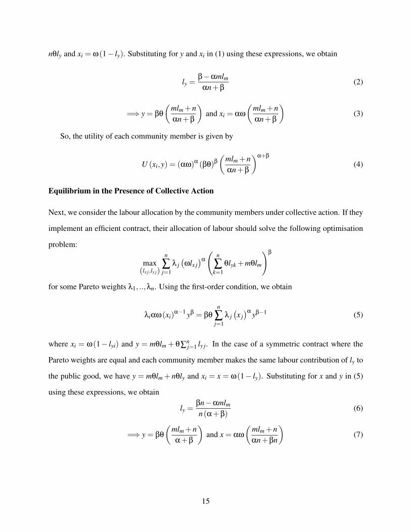
nθly and xi = ω(1− ly). Substituting for y and xi in (1) using these expressions, we obtain

ly =β−αmlm

αn+β(2)

=⇒ y = βθ

(mlm +nαn+β

)and xi = αω

(mlm +nαn+β

)(3)

So, the utility of each community member is given by

U (xi,y) = (αω)α (βθ)β

(mlm +nαn+β

)α+β

(4)

Equilibrium in the Presence of Collective Action

Next, we consider the labour allocation by the community members under collective action. If they

implement an efficient contract, their allocation of labour should solve the following optimisation

problem:

max(lx j,ly j)

n

∑j=1

λ j(ωlx j

)α

(n

∑k=1

θlyk +mθlm

)β

for some Pareto weights λ1, ..,λn. Using the first-order condition, we obtain

λiαω(xi)α−1 yβ = βθ

n

∑j=1

λ j(x j)α yβ−1 (5)

where xi = ω(1− lyi) and y = mθlm + θ∑nj=1 ly j. In the case of a symmetric contract where the

Pareto weights are equal and each community member makes the same labour contribution of ly to

the public good, we have y = mθlm + nθly and xi = x = ω(1− ly). Substituting for x and y in (5)

using these expressions, we obtain

ly =βn−αmlmn(α+β)

(6)

=⇒ y = βθ

(mlm +nα+β

)and x = αω

(mlm +nαn+βn

)(7)

15

So, the utility of each community member is given by

U (xi,y) = (αω)α (βnθ)β

(mlm +nαn+βn

)α+β

(8)

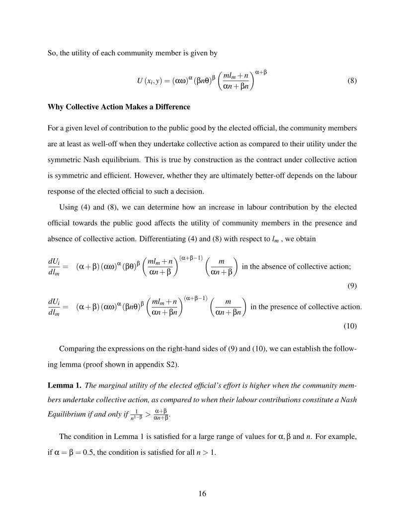
Why Collective Action Makes a Difference

For a given level of contribution to the public good by the elected official, the community members

are at least as well-off when they undertake collective action as compared to their utility under the

symmetric Nash equilibrium. This is true by construction as the contract under collective action

is symmetric and efficient. However, whether they are ultimately better-off depends on the labour

response of the elected official to such a decision.

Using (4) and (8), we can determine how an increase in labour contribution by the elected

official towards the public good affects the utility of community members in the presence and

absence of collective action. Differentiating (4) and (8) with respect to lm , we obtain

dUi

dlm= (α+β)(αω)α (βθ)β

(mlm +nαn+β

)(α+β−1)( mαn+β

)in the absence of collective action;

(9)

dUi

dlm= (α+β)(αω)α (βnθ)β

(mlm +nαn+βn

)(α+β−1)( mαn+βn

)in the presence of collective action.

(10)

Comparing the expressions on the right-hand sides of (9) and (10), we can establish the follow-

ing lemma (proof shown in appendix S2).

Lemma 1. The marginal utility of the elected official’s effort is higher when the community mem-

bers undertake collective action, as compared to when their labour contributions constitute a Nash

Equilibrium if and only if 1n1−β

> α+β

αn+β.

The condition in Lemma 1 is satisfied for a large range of values for α,β and n. For example,

if α = β = 0.5, the condition is satisfied for all n > 1.

16

The Elected Official’s Optimal Choice

Using Lemma 1, we can investigate how the community’s decision about whether or not to under-

take collective action affects the elected official’s labour choice at the second stage of the game.

The official’s optimisation problem can be written as follows:

maxlm

U (xm,y) = (xm)αm (y)βm +π

(1′nU

)Ψ

subject to xm = ωm +ω(1− lm), y = nθly +mθlm and Ui =Ueq for i = 1, ..,n.

Here Ueq is given by (4) in the absence of collective action and by (8) in the presence of

collective action; in addition, ly denotes the equilibrium labour contribution towards the public

good by each community member, given by (2) in the absence of collective action and by (6) in

the presence of collective action, and U′ = (U1,U2, ..,Un).

From the first-order condition to the elected official’s optimisation problem, we obtain the

following, assuming an interior solution:

αmω(xm)αm−1 (y)βm = βmmθ(xm)

αm (y)βm−1 +Ψπ′ (.)

n

∑i=1

dUi

dlm(11)

where π′ (.) is the derivative of the probability function π(.). This equation is identical to that

obtained for ordinary community members except for the last term which derives from the fact

that any effort by the elected official in improving the community’s access to the public good

affects his re-election chances.

We see from Lemma 1 that, for reasonable parameter values, the marginal utility of the elected

official’s effort, dUidlm

(which affects his re-election chances) is higher when the members of the

community undertake collective action. On the other hand, they also allocate a higher level of

effort in the delivery of the public good for any given level of effort applied by the elected official

and this provides the elected official an incentive to free-ride on public good delivery. These two

effects go in opposite directions, and so the net effect on the elected official’s effort is ambiguous.

If the elected official does not directly care for the public good, i.e. βm = 0, then the first effect

17

dominates and he provides higher effort in the delivery of the public good. If βm > 0, the first

effect will dominate if Ψ is sufficiently large; i.e. if he cares enough about being re-elected and/or

the benefits of holding office are sufficiently high. These results are summarised in the following

proposition (proof shown in appendix S2).

Proposition 1. If the conditions in Lemma 1 and Assumption 1 hold and the elected official has

no intrinsic preferences regarding the provision of the public good, then his labour contribution

towards the public good is higher under collective action. If the official cares directly about the

public good, then his labour contribution towards the public good is higher under collective action

if Ψ is sufficiently large.

Thus, assuming the conditions in Proposition 1 hold, the elected official provides a higher

labour contribution towards the public good if the community undertakes collective action at the

first stage of the game. It follows that the community will have a higher level of utility when they

undertake collective action. However, their net gain from collective action also depends on the

fixed cost C. As the cost may vary across communities, some of them may find it in their interest

to form collective action groups while others may not. We discuss this issue in more detail in

Section III.

The Case of Heterogeneous Preferences

Thus far, we have assumed that all members of the community have the same preferences vis-a-vis

their own private consumption and the provision of the public good. In this section, we consider

the setting where the community is composed of distinct groups, which differ in terms of their

preferences regarding public goods. We consider how the elected official’s decisions are affected

when one of the groups organises and engages in collective action to improve the provision of the

public good. We show that the outcome is similar to that obtained in the preceding section.

For ease of analysis, we assume that there are two groups and two public goods. But our main

arguments apply for any number of groups and public goods. We label the two groups in the

population as h and f (for ‘homme’ and ‘femme’), of size nh and n f respectively (nh + n f = n).

18

We label the two public goods as 1 and 2.

If individual i is a member of group g ∈ {h, f}, his/her preferences are given by the following

utility function:

Ug (xi,y1,y2) = (xi)α (y1)

β1g (y2)β2g (12)

where xi denotes the level of i’s private consumption and y1 and y2 denote the level of provision of

public goods 1 and 2 respectively. We impose the following conditions on the preference parame-

ters.

Assumption 2. β1h > β1 f and β2h < β2 f

Assumption 3. β1h +β2h = β1 f +β2 f = β where β ∈ (0,1)

Assumption 2 simply means (without loss of generality) that the male group has a stronger

preference for public good 1 and the female group has a stronger preference for public good 2.

Assumption 3 means that the two groups are alike in terms of their preferences between private

goods and total public goods. We impose Assumption 3 to abstract away from any differences in

behaviour that may arise due to differences in preferences for public goods in general. Note that

Assumptions 2 and 3 allow the preference parameters β2h and β1 f to take negative values. In other

words, the second good may be a ‘public bad’ for men and the first good may be a ‘public bad’ for

women. The preferences of the elected official are defined in a similar manner:

Um (xi,y1,y2) = (xm)αm (y1)

β1m (y2)β2m

As before, he receives a remuneration ωm for his official work and his labour contribution

cannot be contracted upon. He needs to allocate his time between the production of his own

private good and the two distinct public goods. We indicate his labour contributions to his own

private good and the two public goods by lxm, l1m and l2m respectively.

As before, his chances of re-election depends on how well he has served his constituents in the

past. His tenure lasts for one period following which he has to contest elections. His probability of

being successful at the elections is given by π

(λh1′hUh +λ f 1′f U f

)where Uh and U f are vectors

19

describing the utility levels achieved by, respectively, the male and female community members in

the preceding period and 1g is a vector of ones of dimension ng and λh and λ f are positive scalar

terms. Thus, the elected official’s chances of re-election depend on a weighted sum of utilities of

his constituents with all individuals within each gender group assigned the same weight. As in

the case of homogeneous preferences, we assume that the probability function is linear over the

relevant interval:

Assumption 4. π′ (.)> 0 and π′′ (.)= 0 in the interval[λhnhUmin

h +λ f n fUminf ,λhnhUmax

h +λ f n fUmaxf

]where Umin

g and Umaxg are, respectively, the minimum and maximim level of utility that community

members of type g ∈ {h, f} can achieve in the game.18

As in the case of homogeneous preferences, the official’s gain in utility from re-election is

equal to a constant, Ψ. Note that the game can potentially have multiple Nash equilibria because

both men and women can contribute to each public good. To simplify the analysis, we make an

assumption about ‘separate spheres’ of activity for men and women, in the spirit of Lundberg and

Pollak (1993). Specifically, we assume that men can only engage in public action with regard to

good 1 while women can only engage in public action with regard to good 2. This gender division

may be prescribed by social norms so that it is prohibitively costly for women to contribute to

public good 1 or for men to contribute to public good 2, regardless of the preferences within each

group. The timing of events in the game are as described in the case of homogeneous preferences,

but we assume that only the female group has the choice of making the necessary investment for

collective action at the first stage of the game.

Equilibrium in the Absence of Collective Action

First, we consider the case where community members decide on their contribution to the public

good in an uncoordinated manner, and the outcome corresponds to a Nash Equilibrium. Recall that

18To be precise, Uminh =

(nh

αnh+β1h

)α+β1h(

n fαn f +β2 f

)β2hAh, Umin

f =(

n fαn f +β2 f

)α+β2 f(

nhαnh+β1h

)β1 fA f , Umax

h =(m+nhα+β1h

)α+β1h(

m+n fα+β2 f

)β2hAh and Umax

f =(

m+n fα+β2 f

)α+β2 f(

m+nhα+β1h

)β1 fA f , where Ah = (ωα)α (θβ1h)

β1h (θβ2 f )β2h and

A f = (ωα)α (θβ2 f )β2 f (θβ1h)

β1 f .

20

the existence of separate spheres implies that individuals in group h can only contribute to public

good 1 and individuals in group f can only contribute to public good 2. Then, the optimisation

problem for an individual i belonging to group g ∈ {h, f} is given by

maxlxig,lkig

(xig)α (y1)

β1g (y2)β2g

(where k = 1 when g = h, and k = 2 when g = f ) subject to lxig + lkig ≤ 1, xig = ωlxig, y1 =

θ

[ml1m +∑

nhj=1 l1 jh

]and y2 = θml2m +∑

n fj=1 l2 j f .

We restrict our focus to Nash equlibria where all individuals belonging to the same group make

the same labour choices; i.e. lx jg = lxg for g = h, f , l1 jh = l1h and l2 jh = 0, l2 j f = l2 f and l1 j f = 0.

Then, from the first-order conditions, we obtain the following optimisation conditions:

l1h =β1h−αml1m

αnh +β1hand lxh =

αnh +αml1m

αnh +β1hfor men

l2 f =β2 f −αml2m

αn f +β2 fand lx f =

αn f +αml2m

αn f +β2 ffor women

Note that if αml1m > β1h and αml2m > β2 f , then we obtain a corner solution in which the com-

munity members do not make any contributions to the public good. Using the labour contributions

derived above, we can calculate the utility level achieved by men and women in equilibrium for a

given level of labour contribution by the elected official in public goods:

Uh (xh,y1,y2) =

(ml1m +nh

αnh +β1h

)α+β1h(

ml2m +n f

αn f +β2 f

)β2h

(ωα)α (θβ1h)β1h(θβ2 f

)β2h (13)

U f(x f ,y1,y2

)=

(ml2m +n f

αn f +β2 f

)α+β2 f(

ml1m +nh

αnh +β1h

)β1 f

(ωα)α(θβ2 f

)β2 f (θβ1h)β1 f (14)

It should be evident from the expressions that an increase in the elected official’s contribution

to either public good affects the welfare of both groups. But, ceteris paribus, women benefit more

from contributions to public good 2 (since α+β2 f > β1 f ) and men benefit more from contributions

to public good 1 (since α+β1h > β2h).

21

Equilibrium in the Presence of Collective Action

Next, we consider the case where female community members coordinate their actions and choose

the efficient level of contribution to public good 2 (recall that separate spheres implies that they

cannot contribute to public good 1). For any given level of labour allocation by men, an efficient

contract among the women is given by the solution to the following optimisation problem:

max(lxi f ,l2i f )

n f

∑i=1

λi(xi f)α

(y1)β1 f (y2)

β2 f

subject to xi f = ωlx f , y1 = θ

[ml1m +∑

nhj=1 l1 jh

]and y2 = θ

[ml2m +∑

n fj=i l2 j f

].

Here λ1, ..,λn f are Pareto weights. In our analysis, we focus on the symmetric equilibrium

where the utility of each woman is weighted equally and they all make the same contribution to

public good 2; i.e. l2i f = l2 f for i = 1, ..,n f . Similarly, all men make the same contribution to

public good 1; i.e. l1ih = l1h for i = 1, ..,nh. Then, using the first-order condition, we obtain

l2 f =β2 f n f −αml2m

β2 f n f +αn fand lx f =

αn f +αml2m

β2 f n f +αn f

Since collective action enables the group to internalise the externalities provided by their re-

spective contributions to the public good, the level of contribution to the public good is higher. If

men do not undertake collective action, their labour contributions are given by the same equations

as before (we discuss in the next subsection how collective action by men, exogenously deter-

mined, affects the analysis). Using these labour contributions, we can calculate the utility level

achieved by men and women in equilibrium for a given level of labour contribution by the elected

official in public goods:

Uh (xh,y1,y2) =

(ml1m +nh

αnh +β1h

)α+β1h(

ml2m +n f

α+β2 f

)β2h

(ωα)α (θβ1h)β1h(θβ2 f

)β2h (15)

U f(x f ,y1,y2

)=

(ml2m +n f

α+β2 f

)α+β2 f(

ml1m +nh

αnh +β1h

)β1 f

(ωα)α(θβ2 f

)β2 f (θβ1h)β1 f (16)

The presence of collective action by women improves welfare for the male group if β2h > 0

22

and reduces it if β2h < 0. It improves welfare for the female group, and by a greater extent than for

the male group since, by assumption, β2 f > 0 and β2 f > β2h.

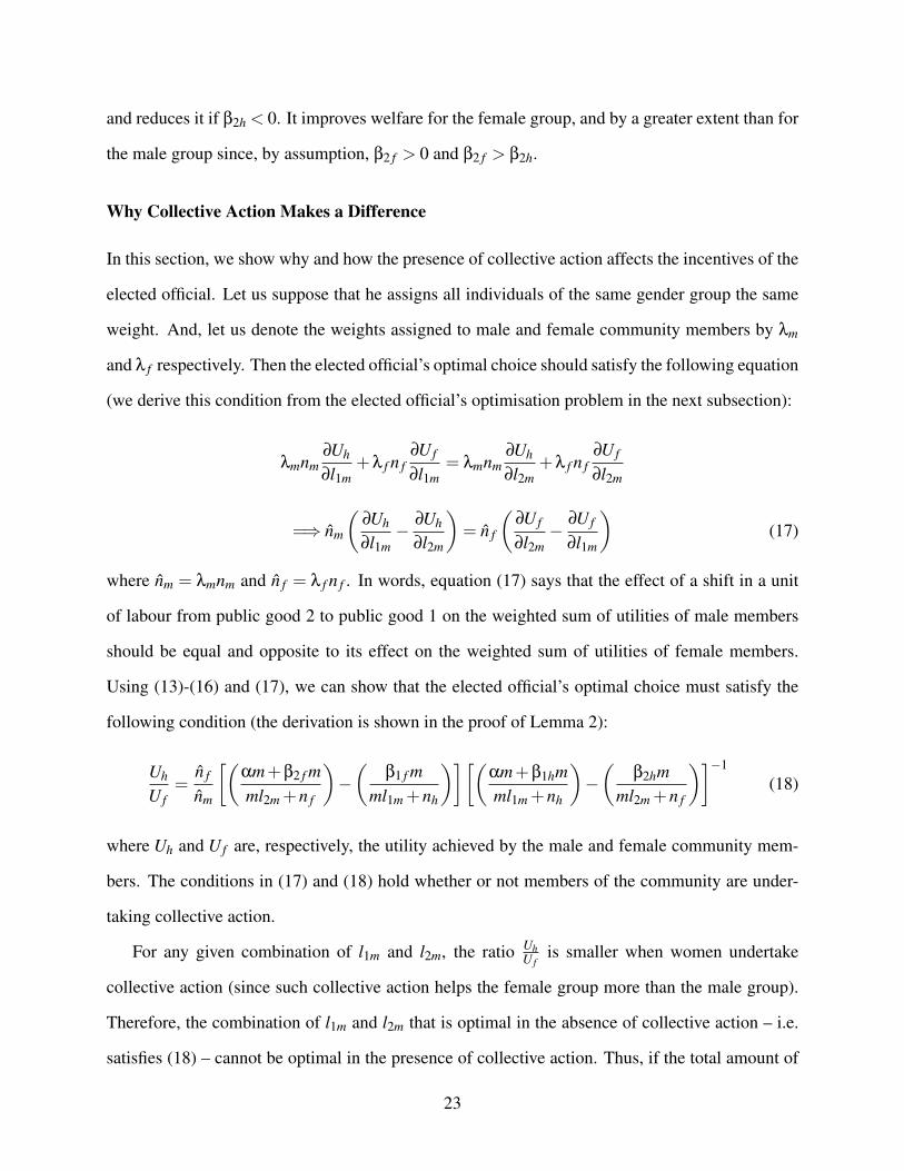
Why Collective Action Makes a Difference

In this section, we show why and how the presence of collective action affects the incentives of the

elected official. Let us suppose that he assigns all individuals of the same gender group the same

weight. And, let us denote the weights assigned to male and female community members by λm

and λ f respectively. Then the elected official’s optimal choice should satisfy the following equation

(we derive this condition from the elected official’s optimisation problem in the next subsection):

λmnm∂Uh

∂l1m+λ f n f

∂U f

∂l1m= λmnm

∂Uh

∂l2m+λ f n f

∂U f

∂l2m

=⇒ nm

(∂Uh

∂l1m− ∂Uh

∂l2m

)= n f

(∂U f

∂l2m−

∂U f

∂l1m

)(17)

where nm = λmnm and n f = λ f n f . In words, equation (17) says that the effect of a shift in a unit

of labour from public good 2 to public good 1 on the weighted sum of utilities of male members

should be equal and opposite to its effect on the weighted sum of utilities of female members.

Using (13)-(16) and (17), we can show that the elected official’s optimal choice must satisfy the

following condition (the derivation is shown in the proof of Lemma 2):

Uh

U f=

n f

nm

[(αm+β2 f mml2m +n f

)−(

β1 f mml1m +nh

)][(αm+β1hmml1m +nh

)−(

β2hmml2m +n f

)]−1

(18)

where Uh and U f are, respectively, the utility achieved by the male and female community mem-

bers. The conditions in (17) and (18) hold whether or not members of the community are under-

taking collective action.

For any given combination of l1m and l2m, the ratio UhU f

is smaller when women undertake

collective action (since such collective action helps the female group more than the male group).

Therefore, the combination of l1m and l2m that is optimal in the absence of collective action – i.e.

satisfies (18) – cannot be optimal in the presence of collective action. Thus, if the total amount of

23

labour allocated to public goods is fixed, the elected official’s optimal allocation of labour involves

a larger l2m and a smaller l1m under collective action. In other words, once the women organise,

the elected official applies more labour in providing the public good that they care about more.

Formally, we have the following result (proof shown in appendix S2).

Lemma 2. Assume that the elected official maximises a weighted sum of utilities of the electorate,

applying the same weight to individuals of the same gender, and the total amount of the elected

official’s labour available for the two public goods is fixed. Assume also that men do not undertake

collective action in the provision of public good 1. Under Assumptions 2 and 3, if women organise

to undertake collective action in the provision of public good 2, the elected official shifts labour

from public good 1 to public good 2, compared to the situation where they do not.

So far we have assumed that the men do not undertake any collective action. A collective

action by men contributing to public good 1 would increase the level of provision of this good and,

therefore, affect the level of utility achieved by both groups. It is straightforward to extend the

analysis above to show that, in such circumstances, a switch by women from a symmetric Nash

equilibrium to collective action would still cause the elected official to shift his labour towards

public good 2. This is shown in Lemma 3 provided in appendix S2.

The Elected Official’s Optimal Choice

Using Lemma 2, we can determine how the female community members’ decision about whether

or not to undertake collective action affects the labour contribution by the elected official. At the

second stage of the game, the elected official’s optimisation problem can be written as follows:

maxl1m,l2m

Um (xm,y1,y2) = (xm)α (y1)

β1m (y2)β2m + π

(λhnhUh +λ f n fU f

)Ψ

subject to xm = ωm +ωlxm, y1 = nθl1y +mθl1m and y2 = nθl2y +mθl2m.

Here l1y and l2y are the equilibrium level of labour contribution to the public goods – and Uh

and U f are the utility levels achieved – by male and female community members respectively, as

derived earlier. Furthermore, lxm = 1− l1m− l2m. From the first-order conditions to the elected

24

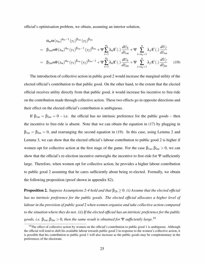
official’s optimisation problem, we obtain, assuming an interior solution,

αmω(xm)αm−1 (y1)

β1m (y2)β2m

= β1mmθ(xm)αm (y1)

β1m−1 (y2)β2m +Ψ

nh

∑i=1

λhπ′ (.)

dUh

dl1m+Ψ

n

∑i=nh+1

λ f π′ (.)

dU f

dl1m

= β2mmθ(xm)αm (y1)

β1m (y2)β2m−1 +Ψ

nh

∑i=1

λhπ′ (.)

dUh

dl2m+Ψ

n

∑i=nh+1

λ f π′ (.)

dU f

dl2m(19)

The introduction of collective action in public good 2 would increase the marginal utility of the

elected official’s contribution to that public good. On the other hand, to the extent that the elected

official receives utility directly from that public good, it would increase his incentive to free-ride

on the contribution made through collective action. These two effects go in opposite directions and

their effect on the elected official’s contribution is ambiguous.

If β1m = β2m = 0 – i.e. the official has no intrinsic preference for the public goods – then

the incentive to free-ride is absent. Note that we can obtain the equation in (17) by plugging in

β1m = β2m = 0, and rearranging the second equation in (19). In this case, using Lemma 2 and

Lemma 3, we can show that the elected official’s labour contribution to public good 2 is higher if

women opt for collective action at the first stage of the game. For the case β1m,β2m > 0, we can

show that the official’s re-election incentive outweighs the incentive to free-ride for Ψ sufficiently

large. Therefore, when women opt for collective action, he provides a higher labour contribution

to public good 2 assuming that he cares sufficiently about being re-elected. Formally, we obtain

the following proposition (proof shown in appendix S2).

Proposition 2. Suppose Assumptions 2-4 hold and that β2h ≥ 0. (i) Assume that the elected official

has no intrinsic preference for the public goods. The elected official allocates a higher level of

labour in the provision of public good 2 when women organise and take collective action compared

to the situation where they do not. (ii) If the elected official has an intrinsic preference for the public

goods, i.e. β1m,β2m > 0, then the same result is obtained for Ψ sufficiently large.19

19The effect of collective action by women on the official’s contribution to public good 1 is ambiguous. Althoughthe official will tend to shift his available labour towards public good 2 in response to the women’s collective action, itis possible that his contribution to public good 1 will also increase as the public goods may be complementary in thepreferences of the electorate.

25

If public good 2 imposes a negative externality on men, i.e. β2h < 0, then the official may not

increase his labour contribution towards the good in response to collective action by women. This

is because collective action by women would not only increase the effect of the official’s labour

on the marginal utility of women but also that on the marginal disutility of men. But, because of

continuity of the functions involved, it can be shown that the results of Proposition 2 will continue

to hold if the negative externality is sufficiently small.

It follows from Proposition 2 that, if the relevant conditions hold, women will achieve higher

utility under collective action (not only because the labour allocation within the group is efficient

but also because the official shifts effort towards the public good for which they have a stronger

preference). Whether this gain in utility is sufficient for them to make the necessary investment for

undertaking collective action at the first stage of the game will depend on the size of the fixed cost

C, as in the case with homogenous preferences. As the cost may vary across communities, women

in some communities may find it in their interest to form collective action groups while others may

not. We discuss this issue in more detail in Section III.

III Implications of the Theory for SHGs and Collective Action

In this section, we discuss the implications of our theoretical results in the context of women’s

SHGs that, as we have discussed, engage in various types of collective action to address issues of

public concern within their ward.

First, it is important to recognise that undertaking collective action involves some fixed costs.

The participating individuals have to agree on what action they will undertake, negotiate about

the division of labour within the group, and setup a monitoring and enforcement mechanism to

minimise free-riding. As discussed in Section I, there is a variety of groups in the PRADAN

villages which undertook collective actions before the NGO began its operations. However, we

found only one women-only group and women play a minor role in the other groups. We argue that

the creation of SHGs provides a space for women to interact in a group on a regular basis, build

26

trust and develop organisational skills, thereby lowering the cost of collective action regarding

ward-level issues of interest to women. The creation of these SHGs thus increases the capacity

of women in the ward to organise and undertake collective action on ‘women’s issues’ in the

subsequent years.

Let us denote by Uvc the utility that women in ward v obtain if they undertake collective action,

as represented by equation (16). Similarly, let Uvn denote the corresponding utility when they do not

undertake collective action, as represented by equation (14). The gain from undertaking collective

action Uvc −Uv

n will vary across wards according to the preferences of the WMs and the divergence

in preferences of his or her constituents. Let us represent the distribution of gains by the c.d.f.

F (.). Following the reasoning in Section II, the theoretical model implies that members of the

SHG would always experience higher welfare when they undertake collective action compared to

when they do not; i.e. F (0) = 0. Let us denote by C0 the fixed cost per woman for engaging

in collective action when they do not have any kind of external organisational support. Given

the absence of women-only groups which undertook collective action prior to the creation of the

SHGs, it seems reasonable to assume that Uvc −Uv

n <C0 for each v; i.e. F (C0) = 1.

The creation of SHGs, we argue, lowered the cost of collective action to Cshg < C0 such that

some fraction of the SHGs found it in their interest to organise themselves and undertake collective

action; i.e. F(Cshg

)< 1.

We argue that, in our empirical setting, the WMs have similar strategic interests to those of the

‘elected official’ considered in the theoretical model. The WMs care about being re-elected and,

therefore, have incentives to take action regarding the public issues that his constituents consider

to be of high priority. On the other hand, the time he spends addressing the ward’s problems and

needs has an opportunity cost in terms of the loss of earnings from alternative income-generating

activities. Furthermore, the WM’s strategic incentives depend on whether his electorate - including

members of SHGs - are capable of undertaking collective action.

As discussed in Section I, SHG members undertake two types of action that complement the

WM’s own efforts: (i) communicating their concerns about a public issue to a higher official; and

27

(ii) intervening directly in the ward. In the empirical analysis, we define the SHG as being active

if the survey records either of these undertakings during the relevant time period.

It should be noted that, for a number of public goods (for example, public infrastructure, wel-

fare schemes, etc.), resources and inputs provided by higher government authorities are an essen-

tial element in their provision. But, in the context of the PRADAN villages, the WMs and citizens

provide an important input for the provision of such goods by identifying problems or ensuring

the quality of delivery. The labour contributions by the elected official and individuals that we

model would correspond to these types of inputs. We do not model the contributions of the higher

authorities explicitly, as our focus is on the strategic interaction between the WMs and citizens.

It is important to note that whether or not a SHG is active is an endogenous variable in our

setting. The SHG may choose not to engage in collective action if, for example, the WM is doing

a satisfactory job of addressing their social concerns. However, the timing of the creation of SHGs

provides an exogenous source of variation in collective action by SHGs. As discussed in Section

I, SHGs generally became active with a time-lag following their creation. This is logical given

that members of the SHG would have to gain expertise regarding its basic operations before it is

able to engage in collective action. Thus, the variation in the timing of SHG creation allows us to

estimate how WMs would respond to exogenous changes in the level of collective action among

their female constituents.

As mentioned in Section I, we do not directly observe the WM’s effort in addressing issues of

interest to his or her constituents. But we do have information on the set of issues regarding which

the SHGs engaged in collective action and the type of issues that the WMs dealt with (see Table

2). Table 3 shows that some issues of concern to the women’s groups, such as ‘alcohol problems’

and ‘school problems’, had been dealt with by very few WMs before the SHGs were created.

Proposition 2 implies that an exogenous increase in collective action increases the WM’s labour

contribution to public issues of interest to women and therefore, in the present context, increases

the probability that the WM tackles such issues.

Relatedly, it should be noted that if there were certain issues of no concern to women’s groups

28

or outside of their sphere of control, then, as per the discussion in Section II, an increase in collec-

tive action by women may cause the WM to decrease his effort in providing them. But we would

not be able to detect the change in our data unless the WM ceased his efforts altogether. This is

unlikely to be the case and we find no evidence of this in the descriptive statistics. Combined with

the reasoning in the previous paragraph, this implies that collective action by the SHGs may have

caused their WMs to increase the number of public issues they dealt with. Thus, the prediction -

based on Proposition 2 - that we test empirically can be summarised as follows.

Prediction 1. An exogenous increase in collective action by women within the ward, due to the

creation of a SHG, would increase the probability that the WM tackles public issues that are of

interest to the group, and would cause the WM to tackle a greater variety of issues.

As discussed in Section I, some PRADAN villages included other groups, primarily composed

of men, which also undertook collective action on a variety of community-level issues. As dis-

cussed in Section II, our theoretical result – on how an elected official responds to the introduction

of collective action by women – holds regardless of whether or not male members of the commu-

nity undertake collective action. Therefore, Prediction 1 is applicable both in communities where

there were pre-existing male groups which undertook collective action on ward-related issues and

in communities where there were not.

IV Empirical Analysis

In this section, we discuss the identification strategy, and formally test the prediction suggested

by the model. To provide further support to our results, we run a placebo regression. Finally, we

present descriptive statistics on the qualitative impact of SHGs’ collective actions.

Identification Strategy

For each ward, we gathered information on the political activities over the past 20 years (four

elections). We asked WMs about the type of issues they dealt with, i.e. the issues for which they

29

visited a higher official or intervened directly in the ward. This allows us to construct a panel for

141 wards.

Consider the following OLS regression to estimate whether the collective actions undertaken

by SHGs have an effect on the activities of WMs:

Ti jt = α1 +α2 SHG activei jt +α3Xi jt +Ct +D j + εi jt (20)

where Ti jt is the total number of different issues that WM i, elected in ward j in year t, deals with.

SHG active is a dummy that takes value 1 if a SHG started undertaking collective actions in ward

j before or during the mandate of WM i. The dummy takes value 0 if no SHG was present in ward

j during the mandate of WM i, or if existing SHGs did not yet start undertaking collective actions.

Xi jt are WM level characteristics, including education level, land ownership, the total number of

children, age, caste category20, and a dummy indicating whether the WM is a man. Ct is a set

of three dummies controlling for the year in which the WM was elected (elected in ’92, ’97, and

’02). The dummies are included to ensure that our variable of interest does not pick up election

year effects, as for example the quality of WMs might increase over time. Finally, D j are ward

fixed effects that control for differences in time-invariant unobservables across wards, and εi jt is

the error term. We cluster the standard errors at the ward level. Our panel is WM specific, so in

case a WM is re-elected, we have information for the full period only (we assumed it would be

difficult for WMs to provide term-wise information).21

The decision of a SHG to become active is potentially endogenous. OLS underestimates the

influence of SHGs on the activities of WMs if SHGs choose not to engage in collective action

because the WM is doing a satisfactory job. On the other hand, OLS overestimates the effect if a

WM particularly sensitive to women issues encourages SHGs to undertake collective actions. As

discussed in Section III, we use the variation in the timing of the creation of SHGs as an exogenous

20Castes are classified in the following categories: ST (scheduled tribe), SC (scheduled caste) and OBC (otherbackward caste) / FC (forward caste).

21To test the sensitivity of our results, we also run regressions in which we include term-wise information. Thedependent variable is the same over the different terms, but the independent variables differ. Our results do not changeusing this different specification.

30

source of variation in the timing of the first collective action by SHGs. Table 4 overviews the

evolution of both the creation of SHGs and their activity over the election periods.

Table 4: The creation and activity of SHGs by election period

Election mandate:1992-1996 1997-2001 2002-2006 2007-2011

% of wards in which at least one SHG has 0.0 42.6 100.0 100.0been created

% of wards in which at least one SHG has 0.0 28.3 68.1 92.9started undertaking collective actions(conditional on a SHG being present)

Source: Authors’ analysis based on data described in the text.

The first SHGs were created during the 1997-2001 election period and, by the end of the 2002-

2006 period, all wards had at least one SHG. As mentioned before, on average, SHGs that under-

take collective actions, do so for the first time after three years of weekly meetings. Therefore, it is

not surprising that most SHGs start undertaking collective actions during the mandates 2002-2006

and 2007-2011.

We will instrument SHG active by whether or not a SHG was created in the ward during the

relevant time period. Our approach leads to the following first stage regression:

SHG activei jt = β1 +β2SHG createdi jt +β3Xi jt +Ct +D j +ζi jt

where SHG created is a dummy that takes value 1 if SHGs were present in ward j during the

mandate of WM i. We use the parameters to predict whether SHGs undertake collective actions,

and estimate consistent estimators for:

Ti jt = δ1 +δ2 SHG activei jt +δ3Xi jt +Ct +D j +θi jt (21)

The assumption underlying this analysis is that the timing of the creation of SHGs is uncor-

related with pre-existing differences in the tendency to intervene for issues across wards, after

controlling for time-varying WM characteristics, time-invariant ward characteristics and a com-

31

mon trend. Next, we assess the plausibility of this assumption.

Exogeneity of the Timing of SHG Creation

In 1994, PRADAN opened an office in the town Keonjhar and started operating in the poorest

block, namely Banspal, which is southwestwards of the town (Figure 1). The initial focus was

on agriculture, as villagers owned some land and small, but perennial rivulets were available to

provide irrigation without the need of major investments. A few years later, in 1998, PRADAN

started promoting SHGs to provide extra resources to strengthen livelihoods.

In the following years, PRADAN identified the poorest regions in the contiguous areas and

expanded its activities. At first, two new offices were opened: one in Suakati, in the Banspal block

in 1998 (Figure 1), and a second in Turumunga, in the Patna block in 1999 (Figure 2). Later,

from 2000 onwards, employees based at the Keonjhar town office started activities in the Keonjhar

Sadar block, located to the west of Keonjhar (Figure 1), and in the adjacent Karanjia block, which

is located in the Mayurbhanj district (Figure 3).

PRADAN’s decision about where to operate was based on the suitability of an area for its

agricultural programs. We surveyed all the wards where PRADAN operates in the Keonjhar and

Mayurbhanj districts of Odisha. Therefore, we believe that, in terms of our research question, the

program placement bias is limited. However, the program timing bias is a concern if the wards in

which PRADAN started working earlier within blocks are systematically different with respect to

the outcomes of interest.

Figures 1, 2 and 3 show the villages in which PRADAN promoted SHGs. We show villages

instead of wards, as ward-level maps do not exist. The villages are a good approximation, as 75%

of the villages encompass exactly the same territory as wards and only 2.8% of the wards cover

several villages. We colored the villages according to the mandate during which a first SHG was

created in the village: 1997-2001 versus 2002-2006.22 We distinguish between these two periods,

as they correspond to the election periods during which SHGs were created (see Table 4). The

22In case there are several wards in the village, we use the mandate during which the first SHG was created in anyof the wards that belong to that village.

32

Figure 1: Keonjhar District: Banspal and Keonjhar Blocks

!.

!.

!.

!.

!.

GH

AS

IP

UR

A

TE

LK

O

I

1

4

2

3

C

H

A

M

P

U

A PA

T

A

N

A

Danla

Deojhar

Kanakana

Kasia

Tentuli

Kusumita

Urumunda

Nelung

Kansa

Kainsi

Ranki

Arsala

Keri

Talajagar

Nayagarh

Kaliapal

Kundei

Naibuga

Basantapur

Ambadahara

Medinipur

Jadipada

Kumundi(KHA)

Tangarpada(Kha)Uparachampei

Goda

Raikala

Potala

Jamunalia

Tikarapada

Khendra

Silisuan

Raisuan

Kasipal

Barigaon

Sendkap

Jharabelada

Suakati

Patbilla

Balibandha

Bhaliadihi

Kaniposi

Ghungi

Naupada

Uparajagara

Toranipani

Poipani

Bhaliadal

Jamudiha(Kha)

Kathabari

Patuakudar

Bistapal

Talapada

Malada

Hatidari

Nuagaon

Jalangadiha

Haridajodi

Dimiria

Talachampei

Gumura

Bramhanidihi

Balabhadrapur

Lunaghara

Sirispal

Sankiri

Chaka

Sanaraduan

Sanhundala

Patung

Balabhadrapur (Alias) Andhari

Kadagarh

Tangarani

Gumura

PurunapaniJoda

Badudighar

Talakainsari

Kalisi

Murusuan

Tulasichaunra

Kanjipani

Sarukudara

Raghunathapur

Chaka

Padmapur

Badaposi

Naradapur

Fakirpur

Durgapur

Rengalbeda

Kunjarabahal

Ichinda

Kodipasa

Kempasada

Gobardhan

Baulamal

Dimbo

Bauripada

Bhaluka

Kaunrikala

Kandarkala

Kendua

Angulia

Ramachandrapur

Kaijoda

Dhatika

Hundula

Murusuan

Banua

Hariharpur

Kandaraposi

Kalanda

Kanaposi

Naigaon

Jamujodi

Dimiridiha

Bodapalasha

Jhumpura

Badaraduan

Nuagaon

Siriskhunta

Mukuna

Khajuripani

Rugudi

Mahadeijoda

Siriabahal

Jhadaposi

Katalposi

Handibhanga

Katupali

Jamuposi

Birakishorpur

Nunajharan

Ghutukesari

Dhenkikot

Jaganathapur

Putulia

Naupani

Aharaposi

Sahadapur

Uparakaipur

Nitigotha

Banajodi

Gopalpur

Rajabasa

Jajapasi

Chingudiposi

Dalimbapur

Kusumila

Tangarani

Deobandha

Danuan

Kasira

Duarasuni

Silisuan

Guhalachatua Khadiadiha

Dimirimunda

Kusapada

Baneikala

Jamudapal

Gopinathapur

Naigaon KaniposiBanpar

Ghuturu

Belapasi

Talakampadihi

Sunariposi

Poipani

Bishnupur

Balisuan

Kulhadihi

Sariaposi

Jamudiha

Maidanikela

Godatopa

Kathabaunsuli

Jamardihi

Gobindapur

Balidiha

Dhanurjayapur

Bramhanjhari

Danardanpur

Teranti

Kotagaon

Dudhakundi

Bajenitangar

Dhudurupala

KhaparakhaiParjanpur

Ramchandrapur alias Balabhadra

Bhatunia

Bhodabahali

Hatikucha

Dhatika

Jagannathapur

Kamalabahal

Sandhiaposi

Dhanurjayapur

Baradapal

Salarapentha

Manoharpur(BADA)

Kholapa

Chhemandibil

Alanapada

Jalapaposi

Sarasakela

Sankarpur

Ghuntapasi

Barkhanda

Sarasa

DhanurjayapurSrirampur

Haladharpur

Upardiha

Sanamuni

Baliaguda

Palashapokhari

Uparasamatha

Ghuntaposi

Ramachandrapur(Kha)

Amunipur

Gopinathapur

Trilochanpur

Tihadiposi

Fakirpur

Andharikhaman

Kumundi(KA)

Tolankabahala

Tolakabahal

Jagannathapur

Bhangabandha

Laxmipasi

Jansonpur

Sarupatala

Madarangajodi

Nahabeda

Teliarsala

Uparakampodihi

Palasapanga

Jalabanga

Narasinghapur

Champadihi

Sarasposi

Kankadajodi

Dabanka

Nischintapur

Basudevpur

Mathuramandali

Jaipur

Padmakesharpur

Kaliabeda

Majuraposi

Manoharpur

Mahuladiha

Kathakaranjia

Balabhadrapur

Dhagotha

Chipinda

Nuadihi

Haladiaguna

Dimiribahala

BaiganposiKajaleipasi

Jadichatar

Satikudar

Mahadebpur

Hirapur

Karanjiapada

Saradhapanka

Mangalapasi

Pratapadhanurjayapur

Ratanpur

Dhaulipat

Mandua

Belada

Chempei

Kesapanka

Podadiha

Nungadia

Bhalupahadi

Deuladiha

Harshapur

Motitangara

Tentulinanda

Amrutapada

Dhatika

Uperkainsari

Tulasipur

Bankamaruni

Haladiatangiri

Jagannathapur

Tangarpalasa

Badamuni

TaratakhamanaPatana

Biswanathpur

Alekhapada

Muktapur

Balabhadrapur

Badbil(Ka)

Govindapur

Sadarapada

Rukunadeipur sasan

Naranapur

Manoharpur

Luhagudi

Singraisuan

Badabil(KHA)

Jamunalia

Khuntapada(GA)

Gopinathapur(nuagaon)

Baghianasa

Jogimatha

Binodabiharipur(Ka)

Boitabeda

Banamalipur

Sundhimurusuan

Atibudhipada

Saharaposi

Spongepatana

Tikargumura

Binodabiharipur(Kha)

Kaliabeda(Baliabeda)

Jamunapasi

Tangarnali

Sankalimati

Basantapur

Nischintapur

Ichhapur

Nirmadapasi

Kendupasi

Biringadihi

Khuntapada(KHA)

Bebartaposi

Goudunibeda

Nuapadmakesharpur

BirabarpurpatanaKhadengapada

Manibandha

Laxmiposi

Jenagadia

Malada

Kodipasa

Suak ati

Kum undi

Nischintapur

Dim bo

Talacham pei

Naranapur

Nuagaon

Nelung

Sank ir i

Raik ala

Kathabar i

Nay agar h

Bal ibandha

Ar sala

Maidank el

Raghunathpur

Talak ainsar i

Nahabeda

Kandarapasi

Handibhanga

Bar adapal

KEONJHAR (M)

Sir ispal

Baur ipada

Raisuan

Par janpur

Basantapur

Mahadei j oda

Palasapanga

Naradapur

Khendra

Gum ura

Gobardhan

Padm apur

Mandua

Kaunr ik ala

Bodapalasa

Jhum pur a

Kutugaon

Janardanapur

Kaunr ik ala

Palasapanga

Malada

Nuagaon

A

A

B

B

C

C

4 4

3 3

2 2

1 1

Orissa Remote Sensing Application CentreDept. of Science and Technology

Govt. of Orissa, Bhubaneswar

CHIEF ELECTORAL OFFICER

Orissa, Bhubaneswar

Sponsored by

!. BLOCK H.Q.

FOREST

MUNICIPALITY / NAC

RIVER / RESERVOIR

G.P. BOUNDARY

VILLAGE BOUNDARY

BLOCK BOUNDARY

ASSEMBLY BOUNDARY NATIONAL HIGHWAY

MAJOR ROADS

OTHER ROADS

RAILWAY

A SSEM B L Y CON STI TU EN CY M A P

24-KEONJHAR (ST)(AS PER DELIMITATION COMMISSION'S ORDER Dt. 15-12-2006)

KEONJHAR DISTRICT, ORISSA

1 - JHUMPURA BLOCK (PART)

2 - BANSPAL BLOCK (PART)

3 - KEONJHAR BLOCK

4 - KEONJHAR (M)

:0 1 2 3 40.5

Kilometers

Legend

Villages where PRADAN entered before the 2002 elections

Villages where PRADAN entered since the 2002 elections

Suakati OfficeSHG promotion since 1998

Keonjhar town officeSHG promotion since 1998

Source: The map was downloaded from http://ceoorissa.nic.in/acmaps.asp (AcNo 24)

33

Figure 2: Keonjhar District: Patna Block

!.

!.

!.

!. !.

!.

!.

C HA

MP

UA

JA

SH

I PU

RK

A

R

A

N

J

I

A

G

H

A

S

I

P

U

R

A

ANAN

DA

PU

R

KE

O

N

J

H

A

R

4

1 2

1

3Sibanarayanpur

TikayatpatnaBadapatna

Sadhupada

Sanapadiaposi

Dumur ia

2

Udayapur

Baunsuli

Erendei

Bhulada

Bala

Asanapat

Tando

Khamua

Baikala

Begana

SilipadaGorasa

Gundunia

Saraskola

Musakhori

Silida

TandoDumuria

Khadikapada

Kumudabahali

Rudhiapada

Kapundi

Gidhibas

Denua

Kantiapada

Baria

Kalinga

Tukudiha

Ankura

Chinamalpasi

Lunga

Khireitangiri

Jumei

Bila

Sirikuan

Kundala

Kendua

Solagoda

Raikala

ChemanaPodasimila

Madhapur

Raipur

Baikunthapur

Chilida

Asuria

Dianali

Banabir

Dabarchua

Nuagaon

Badapasi

Jally

Mahuldiha

Ninhua

Raidiha

Jamuda

Tangarpada

Jamunapasi

Tangarpada

Kamaramara

BinindaHatibari

Sialijoda

Digaposi

Chutiaposi

Jayipur

Ostajodi

Nuapada

Dalanga

Baratunia

Sadangabahali

Manpur

Banmahuldiha

Manada

Barakhandia

Bhodaposi

Gorandijodi

Mahisamundi

Godipokhari

Saradhapur

Badajamupasi

Sadangi

Putulia

Tribindha

Gandabarei

Nuapada

Balibandha

Telipada

Tentala

Baruna

Tendara

Kudabeda

Baunsanali

Pipilia

Badaneuli

Purunapani

Ghatbalijadi

Golakunda

Neundi

Kaunrikala

Jyotipur

Chauthia

Kendeipasi

Gojitangar

Dhatika

Baliapasi

Angikala

Khuntapada

Chatarpani

Gopiballavpur

Mirigikhoji

Palanghati

Jamunalia

Laxmiposi

Damahuda

Kendujoda

Fulapahadi

Dalapaka

Bhimapur(Bhuinpur)

Putugaon

Maudipa

Ketanga

Hirapasi

Jadichatar

Malarpada

Aharapada

Panuposi

Parsala

Katabeda

Khuntapada

Khadibeda

Medinipur

Tavasarua

Baliposi

Guludipasi

Ukhunda

Badabil

Dhanabeni

Bhaliadal

Bananipasi

Duaghata

Sankhua

Nischintapur

KaindaPahadpur

Barhaposi Belapasi

Ankudi

Pichhilabeda

Gopinathpur

Jamunalia

Kothaghar

Rengalabeda

Machhagarh

Brahmanideo

Purunia

Kodakhamana

Paitamaja

Hariposi

Murusuan

Tangarbantala

Sananeuli

Badaposi

Kashipur

Chhelianal

Khuntapingu

Sarasinga

Budhikapudi

Balitota

Mahadevpur

Maliposi

Gandibeda

SunaposiBhalughar

Talapada

Pingupatana

Badagahmaria

Chitrapur

Jajaposi

Silitia

Sijukala

Kaliaduma

Nagarpal

Belasarei

Patanali

Katuposi

Saraspasi

Sanabaliposi

Gidhibasa

Khuntapada

Baradangua

Kankada

Bandhanahara

Tentalapasi

Ashoki

Khuntapada

Chadeibhure

Rengalbeda

Badadumuria

Dobeipentha

Palasapada

Badnuagaon

Bhalupahadi

Jamuleibeda

Fulkanlei

Nuakhamana

Baidabaza

Keshadiha

Jhaliapada

Kenduapada

Madhupur

Khajuriapata

Radhapur

Pichhulabeda

Jarakanibeda

Rasabantala

Chakundapal

Padmapur

Badadhanurjayapur

Balipasi

Barudipasi

Bhaliadiha

Gainsiri

Dasharathipur

Kanchandumuria

Kucheibeda

Nischintapur

Banmalipur

Kantidiha

Kamanda(KA)

Balaniposi

Bhanrapur

Godheinali

Saharapada

Gayalkund

Budhabana

Sanagahmaria

Purandarpur

Rajanagar

Gobindpur

Bhangabilla

Sitarampur

Gunduriposi

Parbatipur

Tilabeda

Khudaposi

Talapada

Muktapur

Bhurupada

Nayadhanurjaypur

Turumunga

Khandeipada

Dasapada

Padhanpada

Hariharpur

RasapadaMusapada

Khajuridiha

Dudhanali

Chakulia(Chakadiha)

Mangalapur

Nuagaon (Bada)

Bhubanposi

Godhirampara

Gajapathar

Danuatangarpada

Bhimapada

Neudipasi

Birikuan(KA)

Barachela

Rohaniduma

Haridagotha

Kashipur

Tentulikhunti

Tentala

Nuagaonkhilaripata

Jaganathapur

Saraswatipada

Galaphula

Mangalapur

Ratanpur

Parudiposi

Kimirdapasi

Suagapur

Barabeda

Nischintapur

Sankhasara

Kumudabahali

Laxmiposi

Deuliapasi

Laxmiposi(Ka)

Khajuriapasi

Singmajuni

Padiapasi

Jamunaposi

Mandama(Manima)

Kiapada

Bardhana

Birikuan(KHA)

Tainsira

Sanadhanurjaypur

Talasarua

Bhandaribila

Sabaranibeda

Asanabani

Hastinapur

Uchatanagar

Nuagaonbalavadrapur

Panapasi

Gobindapur

Banapada

Kalighai

Sunariposi

Padmakesharpur

Asanabahali

Harichandanapur

Karanjiapada

Analadiha

Katupada

Ratnaposi

Ghungibeda

Arjunpur

Kuapasi

Badabaliposi

Saharaposi

Bhrungaraj

Nuabandha

Nayabandha

Janheipasi

Ramachandrapur

Balabhadrapur

Ganiabarei

Surendrapur

Budhimara

Hatianasa

Matiaguni alias gopalpur

Ramachandrapur

MayurapankhaJharabeda

Bichitranandapur

Dumurigoda

Dhanurjaypur

Beguniapasi

Bhogapasi

Hinjalagadia

Dharuapada

Suambirajayagovindpur

Gopinathapur

RadhikadeipurManoharpur

Lekhana

Patadhanurjayapur

Deogaon

Haladibata

Kameswarpur

Kamanda(KHA)

Sabak Dhanurjaypur

Nayajaganathapur

Shyamsundarpur

Giliriduma

Raghunathapur

Jagannathapur

Giridhina

kantaposi

Nuagaonbudhusahi

Chuapani

Banakati

Ranipur(KA)

Vaga bandha

Chaitanpur

Kochilapada

Changuapada

Ramachandrapur

Rathapada

Sanajamuposi

Bautiapada

Tangarnali alias Rauturapur

Kodadhara

Bhabisakudar

Badapadiapasi

BalipokhariKakharuabeda

DurgadeipurKamalabahali

Govindapur

Nakanlei

Dwitiya Sivanarayanpur

Dumuridiha

Narayanpat (Naranpat)

Jal l y

Baunsul i

Bar ia

Bar bi l

Asanpat

ChemanaBaik ala

Sahar padaUday apur

Dumur ia

Bhuinpur

Tuk udiha

Goras

Kendeipasi

Tangarpada

Palanghat i

Si l ipada

Raid iha

Badaneul i

Badapatna

Khuntapada

Digiposi

Machhagar h

Dalapak a

Erendei

Chauth ia

Jaj aposi

Mal lar pada

Kapundi

Sarasak ola

Chinamal ipasi

Kantiapada

Khaj ir apat

Budh ik apud i

Uk hunda

Musak hor i

Jamunaposi

Kundala

Gandabeda

Khirei tangir i

Tendara

Sank hua

Khadik apada

Murusuan

Raj nagar

Damahuda

Turum unga

Khuntapada

Chak undapal

Sadangi

Gundunia

Dumur ia

Par sala

Mir igi k hoj i

Jy ot ipur

Dhanur jay apur

Badadum ur ia

Dhanur jay apur

Par sala

Tendara

Jy ot ipur

Tuk udiha

Dumur ia

Jy ot ipur

A

A

B

B

C

C

4 4

3 3

2 2

1 1

Orissa Remote Sensing Application CentreDept. of Science and Technology

Govt. of Orissa, Bhubaneswar

CHIEF ELECTORAL OFFICER

Orissa, Bhubaneswar

Sponsored by!. BLOCK H.Q.

FOREST

MUNICIPALITY / NAC

RIVER / RESERVOIR

G.P. BOUNDARY

VILLAGE BOUNDARY

BLOCK BOUNDARY

ASSEMBLY BOUNDARY NATIONAL HIGHWAY

MAJOR ROADS

OTHER ROADS

RAILWAY

A SSEM B L Y CON ST I T U EN CY M A P23-PATNA (ST)

(AS PER DELIMITATION COMMISSION'S ORDER Dt. 15-12-2006)

KEONJHAR DISTRICT, ORISSA

:0 2 4 6 81

Kilometers

1 - JHUMPURA BLOCK (PART)

2 - CHAMPUA BLOCK (PART)

3 - PATNA BLOCK

4 - SAHARPADA BLOCK

LegendVillages where PRADAN entered before the 2002 elections

Villages where PRADAN entered since the 2002 elections

Turumunga officeSHG promotion since 1999

Source: The map was downloaded from http://ceoorissa.nic.in/acmaps.asp (AcNo 23)

34

Figure 3: Mayurbhanj District: Karanjia Block

!.

!.

!.!.

!.

!.

!.

!.

!.

!.

!.

!.

!.

!.

2

1

4

3

JA

SH

IP

UR

B

A

N

G

IR

IP

O

S

H

I

UD

AL

A

P

A

TA

NA

A

N

A

ND

AP

UR

GHASIPURA

AN

AN

DA

PU

R

SM

UL

IA

NI

LG

I

R

I

Badgaon

Salchua

Salchua

Nota

Kesdiha

Duara Suni

Sarat

Dhapada

Bhandar

Dewanbahali

Taramara

Jarak

Mituani

Bala

Boring

Dugudha

Satkosia

Bisipur

Rajatnagar

Nada

Dari

Ghulghulia

Mata

Patbil

Bhaliadal

Katuria

Sarubil

DolipadaTolagadia

hatigoda

Saradiha

Dakeipal

Purunapani

Kadabahali

Kunjia

Ranipokhari

Ghosda

Gokulpur

Kerkera

Paudia

Simdiha

Pingu

Dirba

Goudia bahali

Jamunanda

Bharandia

Sukhuapata

Gourchandrapur

Digdhar

Dumuria

Chheratangar

Bhanra

Labanyadeipur

Kaliajiani Ranibhol

Siriapal

Nuagan

Kurulia

Halpur

Jamunalia

Diliganj

Saradha

Tikasil

Dillisahar

Padiabeda

Baghadafa

Gahandiha

Ghodabindha

Balibhal

Baunsadiha

Koliposi

Kendumundi

Chirupada

Kumudabadi

Nuagan

Baghadafa

Talapada

Ramchandrapur

Dangadiha

Nakuda

Handifuta

Balichua

Kalakada

Tuntuna

Salachua

Miludihi

Mulapal

Murgapat

Baliposi

Dihajodi

Chakulia

Kia

Jadibil

Saradha

Padeidhuda

Kelarposi

Bisungaon

Radang

Kathakaranjia

Panaposi

Bhejidiha

Banki

Jarali

Sukhuapata Hill

Kham Diha

Kalamgadia

Badbaliposi

Tata

Saleibeda

Padmapokhari

Badadeuli

PrasanachandrapurMahuldiha

Nedhuapal

Jhadbeda

Edelbeda

Sarangagad

Gaudgan

Asanbani

Biunria

Purunapani

Khejuria

Sunariposi

Khudsila

Purunapani

Rengalbeda

Kadadiha

Batapalasa

Satkosia Forest cluster

Pahadmadak

Patiapada

Bhadubeda

Raipada

Singada

Deogan

Miriginandi

Kadapani

Kankada

Rasamtala

Ramjodi

Gidhibas

Kenjhara

Asanbani

Burudihi

Dangapani

Baghadafa

Bandhagan

SalarapadaHatibari

Sripadamanjaripur

Jangal Block Samil Sudarsanpur

Nuagan

Jamuposi

ChamakpurDaunikila

Jamunalia

Kusapada

Nipania

Sanadeuli

Godabhanga

Panaspal

Ghantiadara

Jalada

Dumurdiha

Jhalakiani

Guliajodi

Khaparkhai

Sarasaposi

Kendujiani

Nuapada

Mandua

Oriam

Nundiha

Kirikichipal

Hatisalbeda

Ranibhol

Jodipada

Dhatikidiha

Kuduma

Kalasira

Simgan

Jhaddumuria

Majuraposi

Ghadaghagudi

Kucheikudar

Khadipal

Sanbadapasi

Badbil

Ranipat

Suninda

Khumthan

Sunaposi

kathachua

Mandal Jhari

Laxmiposi

Chheliaposi

Karadia

Anlakata

Basantpur

Thakurmunda

Patulidiha

Dumbisahi

Giribeda

Badaposi

Jamukhanjari

Jamunalia

Andarjhari

Pariarsahi

Baliposi

Dudhiani

Chainbainsi

Chadhaibhol

Tikarpada

Guhaldihi

Akhapolan

Pakamunda

Tulasiposi

Godidiha

Banamunda

Malharpada

Asankudar

Nuagaon

Khalpada

Kasibeda

Patarpada

Pichhuli

Sarabhadi

Kaliaposi

Badagan

Khadidamak

Jadidar

Gobarjoda

Kucheidiha

Kapandara

Barapanposi

Dibigarh

Thakurjharan

Bhairanibeda

Jhatiali

Kadambeda

Champajhar

Gourigoda

Baula

Bhadubeda

Khadikudar

Tulasiposi

Chauthia

Rugudisahi

Dubapal

Sanadei

Bhanraposi

Khandbandh

Satabedi

Jarasahi

PahadbhangaKiapanposi

Dhakata

Chanchabani

Badmahuldiha

Mukundiapada

Kudarsahi

Chaturisahi

BaliposiAmbabeda

Kadalibadi

Ramachandrapur

Hatidandi

Kathuanuagaon

Mankadabeda

Satakiari

Miriginendi

Nischintapur

Thianali

Badasarai

Baliabeda

Dhatikibeda

Khasakudar

Nuapada

Asanbani

Nisaposi

Karadapal

Badramchandrapur

Jadibeda

Sanagansasan

Batatainsira

Bhalugodaorofchitraposi

Khuntakata

Raitalia

Kadamadak

Gaipanikhiahill

Budhigan

Rugudibeda

Jamudiha

SialinaiDhalabani

Kokanda

Khuntaposi

Baunsa Pani

Syamchandrapur

Balidiha

Madarangajodi

Sanmohuldiha

Antasahi

Sanandharilkhaman

Mahadevdeuli

Baghamunda

Khandiadar

Purunadeogan

Sudiam

Dhirol

Kanjiapal

Batagaudagan

Bajenisila

Prafullachandrapur

Gapalpur

Purunapani

Jambani

Badposi

Bhalughar

Kasibania

Panasa diha

Jhumukakudar

Baghalata

Ranibholorofkalodar

Sanarugudibeda

Thakuramapatana

Nadhagadia

Sanbarahkamuda

Nihangandi

Bholpada

Pahadpur

Dangasila

Sanramchandrapur

Betajhari

Lokanathpur

Sanbaliposi

Sadangitainsira

Asurkhal

Rangamatia

Raidiha

Jharjhari

Baghamara

Bhandaribila

Ambaduma

Badbarahkamuda

Kundei

Danuabaliposi

Birajadunathpurshasan

Chaulajhari

Satkosiaamal Nama Hill Block

Patbil

Bahaghar

Meghasani

Kandadhanu

Debasthali

Nuagaon

Upper Barahakamuda

Dari

Patbil

Satkosia

Nota

Jarak

Kuliposi

Sarat

Bala

Keshdiha

Talpada

Hatigoda

Tato

Baddeuli

Dudhiani

Sardiha

Padiabeda

Kendujiani

Kalamgadia

Saleibeda

Rasantala

Bharandia

Khandabandha

Ranipokhari

Mahuldiha

Dewanbahali

Batpalsa

Bhaliadal

Padmapokhari

Ramachandrapur

KARANJIA (NAC)

Kerkara

Digiddhar

Champajhar

Chitraposi

Thakurmunda

Miriginandi

Labanyadeipur

Hatigoda

Hatigoda

Champajhar

Hatigoda

Hatigoda

Saleibeda

A

A

B

B

C

C

D

D

E

E

4 4

3 3

2 2

1 1

1. KARANJIA BLOCK2 THAKURMUNDA BLOCK3. KAPTIPADA BLOCK (PART)4. KARANJIA (NAC)

Orissa Remote Sensing Application CentreDept. of Science and Technology

Govt. of Orissa, Bhubaneswar

CHIEF ELECTORAL OFFICEROrissa, Bhubaneswar

Sponsored by!. BLOCK H.Q.

FOREST

MUNICIPALITY / NAC

RIVER / RESERVOIR

G.P. BOUNDARY

VILLAGE BOUNDARY

BLOCK BOUNDARY

ASSEMBLY BOUNDARY NATIONAL HIGHWAY

MAJOR ROADS

OTHER ROADS

RAILWAY

:0 3 6 9 121.5

Kilometers

A SSEM B L Y CON STI TU EN CY M A P30-KARANJIA (ST)

(AS PER DELIMITATION COMMISSION'S ORDER Dt. 15-12-2006)

MAYURBHANJ DISTRICT, ORISSA

Karanjia officeSHG promotion since 2000

LegendVillages where PRADAN entered before the 2002 elections

Villages where PRADAN entered since the 2002 elections

Source: The map was downloaded from http://ceoorissa.nic.in/acmaps.asp (AcNo 30)

35

maps reveal two important patterns. First, all PRADAN offices in all blocks created SHGs both

before and after the 2002 elections. Second, the villages in which SHGs were created earlier

and later are neighboring one another. This is the result of PRADAN’s preference for having the

same employee operate in the same villages over time: each employee is assigned a cluster of

neighboring villages in which he creates SHGs following the pace and the direction he considers

appropriate. This policy saves traveling time and limits transportation costs. We address potential

employee biases by including ward fixed effects. As the villages in which PRADAN created SHGs

before 2002, and those in which SHGs were created later are situated close together, it is likely

that they have similar socioeconomic characteristics. We check whether this is indeed the case in

the Tables 5 and 6.

Table 5 displays data from the 1991 Census of India. The village is the lowest level at which

data is available, so we cannot do a ward-level comparison. We could match all but three villages

(105 total). The first column provides details on villages in which the first SHG was created during

the 1997-2001 mandate, the second column on villages that had a first SHG created during the

2002-2006 mandate, and the third column provides the difference. With the exception of power

supply, there are no significant differences for a wide range of facilities and public infrastructures.

Villages also have, on average, the same size, and similar rates of employment, and literacy.

We also used all the variables in Table 5 to predict SHG creation (a dummy taking value 1 (0)

if the first SHG was created in 2002-2006 (1997-2001)). We cannot reject the joint null hypothesis

(p-value = 0.64).23 This result provides an argument in favor of SHG creation not being influenced

by the elected WMs.

Next, Table 6 shows the outcome variables and controls of our main regressions for the period

1992-1996, i.e. before the first SHGs were created, at the ward level. Although the number of ob-

servations is limited, the difference is small for all variables, but for welfare schemes. Furthermore,

the sign is not systematically positive or negative.24

23The regression is available upon request.24We excluded the WMs who have been re-elected in 1997 and faced SHGs undertaking collective actions, since

for them we do not have disaggregated information. This reduces the number of observations, but allows us to compareinformation on WMs before SHGs were active.

36

Table 5: Village characteristics based on the Census of India 1991, by mandate during which a first SHGwas created in the village

First SHG created in the village in1997-2001 2002-2006 Difference(Std. Dev.) (Std. Dev.) (Std. Err.)

Number of households 129.3 112.4 16.9(83.2) (84.5) (16.5)

Literacy rate of women 12.3 15.5 -3.2(9.5) (10.9) (2.0)

Literacy rate of men 33.1 37.6 -4.5(16.0) (17.2) (3.3)

Employment rate of women 18.8 16.3 2.5(15.8) (16.9) (3.2)

Employment rate of men 53.6 51.9 1.7(5.2) (9.3) (1.5)

EDUCATION FACILITIESNumber of primary schools 0.87 0.78 0.09

(0.40) (0.46) (0.09)Number of middle schools 0.24 0.14 0.10

(0.43) (0.39) (0.08)Number of high schools 0.13 0.07 0.06

(0.34) (0.31) (0.06)

MEDICAL FACILITIESA medical facility is available (% of villages) 15.2 6.8 8.4

(36.3) (25.4) (6.0)

DRINKING WATER FACILITIESWell water (% of villages) 73.9 83.1 -9.2

(44.4) (37.8) (8.0)Tank water (% of villages) 45.7 54.2 -8.5

(50.4) (50.2) (9.9)Tube well (% of villages) 30.4 32.2 -1.8

(46.5) (47.1) (9.2)River water (% of villages) 28.3 20.3 8.0

(45.5) (40.6) (8.4)

OTHER INFRASTRUCTUREBus stop (% of villages) 17.4 13.6 3.8

(38.3) (34.5) (7.1)Village accessibility by paved road (% of villages) 28.3 25.4 2.9

(45.5) (43.9) (8.8)Market facility available (% of villages) 13.0 6.8 6.2

(34.1) (25.4) (5.8)Power supply (% of villages) 54.3 71.2 -16.9∗

(50.4) (45.7) (9.4)Irrigated land (% of land) 5.2 6.1 -0.9

(11.4) (17.6) (3.0)

Number of villages 46 59∗∗∗ significant difference at 1 percent, ∗∗ significant difference at 5 percent, ∗ significant differ-ence at 10 percent.Source: Authors’ analysis based on data from the Census of India, 1991.

37

Table 6: Summary statistics at baseline (1992-1996), by mandate during which a first SHG was created

First SHG created in the ward in1997-2001 2002-2006 Difference(Std. Dev.) (Std. Dev.) (Std. Err.)

DEPENDENT VARIABLES FOR 1992-1996Number of ward problems addressed by the WMs 1.42 1.36 0.06

(0.87) (1.09) (0.23)WM deals with alcohol issues (%) 0.0 2.6 -2.6

(0.0) (16.0) (2.8)WM deals with school issues (%) 6.1 7.7 -1.6

(24.2) (27.0) (6.1)WM deals with forest issues (%) 18.2 23.1 -4.9

(39.2) (42.7) (9.7)WM deals with public infrastructure (%) 78.8 71.8 7.0

(41.5) (45.6) (10.4)WM deals with welfare schemes (%) 39.4 25.6 13.8

(49.6) (44.2) (11.1)

CHARACTERISTICS WMs IN 1992-1996(= independent variables)Male (%) 87.9 79.5 8.4

(33.1) (40.9) (8.9)Education level (years) 4.9 6.8 -1.9∗∗

(3.1) (3.7) (0.8)Land (acres) 3.0 3.2 -0.2

(2.0) (7.8) (1.4)Number of children 3.7 3.1 0.6

(1.8) (1.8) (0.4)Age 58.8 52.3 6.5∗∗

(11.1) (12.2) (2.8)Caste category: SC (%) 6.1 7.7 -1.6

(24.2) (27.0) (6.1)Caste category: OBC/FC (%) 12.1 25.6 -13.5

(33.1) (44.2) (9.4)

Number of wards 33 39∗∗∗ significant difference at 1 percent, ∗∗ significant difference at 5 percent, ∗ significant differ-ence at 10 percent.Source: Authors’ analysis based on data from the Census of India, 1991.

38

Results

First, we measure the impact of SHGs on the number of different problems a WM deals with.

The results are shown in Table 7. The columns (1) and (2) provide the estimates using OLS

(equation 20), and the columns (3) and (4) using instrumental variables (equation 21). Regressions

without WM controls are provided in the odd-numbered columns and those with controls in the

even-numbered columns.

WMs operating in wards where SHGs have started undertaking collective actions deal with

1.5 extra issues compared to WMs who operate in wards where SHGs are not present or do not

undertake actions. The result confirms our prediction: an increase in collective actions within the

ward causes the WM to tackle a greater variety of issues. The coefficients are significant, but

slightly smaller in size in the OLS regressions. We also find that, overall, male WMs deal with

fewer issues.

Next, we examine the type of extra issues the WM starts dealing with. To do that, we replace

the left hand side variable of the equations (20) and (21) by Ti jtk, a dummy equal to one if WM

i, elected in ward j in year t, deals with issue k. The independent variables are the same. The

results are given in Table 8. The odd numbered columns provide the results using OLS, and the

even numbered columns using IV.

Once SHGs undertake collective actions, WMs are 29% more likely to deal with alcohol prob-

lems, 31% with school problems and 35% with forestry issues. WMs are also more likely to start

dealing with welfare schemes. Thus, the estimates confirm that WMs start dealing with public

goods that are of interest to SHGs (see Section I). The bias is similar to the previous regression:

The IV coefficients are close to or larger than their OLS counterparts.

Interestingly, male WMs are less likely to take care of alcohol issues, school problems and

welfare schemes, but they are more likely to deal with public infrastructure.

39

Table 7: The effect of collective actions by SHGs on the number of issues addressed by the WM

Number of issues addressed by the WMOLS 2SLS

(1) (2) (3) (4)

SHG active 0.89∗∗∗ 0.91∗∗∗ 1.48∗∗∗ 1.54∗∗∗

(0.16) (0.16) (0.42) (0.42)Male -0.29∗∗ -0.33∗∗∗

(0.12) (0.13)Education level (years) 0.03 0.03

(0.02) (0.02)Land (acres) -0.04∗∗∗ -0.04∗∗∗

(0.01) (0.01)Number of children -0.02 -0.01

(0.03) (0.03)Age 0.05∗ 0.05∗

(0.03) (0.03)Squared age -0.00∗ -0.00

(0.00) (0.00)Caste category: SC -0.16 -0.12

(0.21) (0.23)Caste category: OBC/FC 0.02 0.06

(0.16) (0.17)

Ward fixed effects yes yes yes yesElection year dummies yes yes yes yesF-stat first stage 31.6 29.1Observations 441 441 441 441

An observation in the regression model is a WM. The dependentvariable is the total number of different issues that the WM deals withduring his mandate. The variable “SHG active” is a dummy that takesvalue one if a SHG started undertaking collective actions in ward j beforeor during the mandate of WM i. The first two columns provide the resultsusing standard linear regression techniques. In the last two columns weinstrument for “SHG active”, using the timing of SHG creation in theward. The uneven columns do not include WM characteristics, while theeven columns do so. Standard errors clustered at the ward level are givenin parentheses. *** significant at 1 percent, ** significant at 5 percent, *significant at 10 percentSource: Authors’ analysis based on data described in the text.

40

Table 8: The effect of collective actions by SHGs on the type of issues WMs deal with

Probability that the WM deals with:Alcohol issues School issues Forest issues Infrastructure Welfare scheme

OLS IV OLS IV OLS IV OLS IV OLS IV(1) (2) (3) (4) (5) (6) (7) (8) (9) (10)

SHG active 0.30∗∗∗ 0.29∗∗ 0.19∗∗∗ 0.31∗∗ 0.22∗∗∗ 0.35∗∗ 0.04 0.10 0.14∗ 0.40∗

(0.06) (0.14) (0.06) (0.14) (0.05) (0.17) (0.07) (0.21) (0.08) (0.23)Male -0.11∗∗∗ -0.11∗∗∗ -0.07 -0.08∗ -0.06 -0.06 0.09∗ 0.09∗ -0.14∗∗∗ -0.16∗∗∗

(0.04) (0.04) (0.04) (0.04) (0.04) (0.04) (0.05) (0.05) (0.05) (0.06)Education level (years) 0.01∗∗ 0.01∗∗ -0.00 -0.00 -0.01 -0.01 0.00 0.00 0.01 0.01

(0.01) (0.01) (0.01) (0.01) (0.01) (0.01) (0.01) (0.01) (0.01) (0.01)Land (acres) -0.01 -0.01 -0.01∗∗∗ -0.01∗∗∗ -0.01 -0.01 -0.01 -0.01 -0.00 -0.00

(0.01) (0.01) (0.00) (0.00) (0.01) (0.01) (0.01) (0.01) (0.01) (0.01)Number of children -0.02∗∗ -0.02∗∗ 0.01 0.01 -0.00 0.00 -0.03 -0.03 0.01 0.01

(0.01) (0.01) (0.01) (0.01) (0.01) (0.01) (0.02) (0.02) (0.01) (0.01)Age 0.00 0.00 0.01 0.01 0.00 0.00 0.02∗ 0.02∗ 0.02∗ 0.02

(0.01) (0.01) (0.01) (0.01) (0.01) (0.01) (0.01) (0.01) (0.01) (0.01)Squared age 0.00 0.00 -0.00 -0.00 -0.00 -0.00 -0.00 -0.00∗ -0.00∗ -0.00∗

(0.00) (0.00) (0.00) (0.00) (0.00) (0.00) (0.00) (0.00) (0.00) (0.00)Caste category: SC -0.08 -0.08 0.05 0.06 -0.12 -0.12 -0.10 -0.10 0.11 0.13

(0.06) (0.06) (0.08) (0.08) (0.08) (0.08) (0.09) (0.09) (0.11) (0.11)Caste category: OBC/FC -0.14∗∗ -0.14∗∗ 0.08∗ 0.08∗∗ -0.03 -0.03 -0.01 -0.01 0.16∗∗ 0.18∗∗

(0.06) (0.06) (0.04) (0.04) (0.05) (0.05) (0.05) (0.05) (0.07) (0.07)

Ward fixed effects yes yes yes yes yes yes yes yes yes yesElection year dummies yes yes yes yes yes yes yes yes yes yesObservations 441 441 441 441 441 441 441 441 441 441

An observation in the regression model is a WM. The dependent variable is a binary variable that equals one if the WM deals with the issueduring his mandate. The variable “SHG active” is a dummy that takes value one if a SHG started undertaking collective actions in ward j before or duringthe mandate of WM i. The odd numbered columns provide the results using OLS. In the even numbered columns we instrument for “SHG active”, usingthe timing of SHG creation in the ward. Standard errors clustered at the ward level are given in parentheses. *** significant at 1 percent, ** significant at 5percent, * significant at 10 percent.Source: Authors’ analysis based on data described in the text.

41

Placebo Regression

In this section, we perform a placebo regression. SHGs become active during the election periods

2002-2006 and 2007-2011 in 78% of the wards. Before 2002, there should not be differences

between wards where SHGs started undertaking collective actions in 2002-2006 as compared to

those in which SHGs became active in 2007-2011. To test this, we restrict our data set to WMs

whose mandate finished before 2002, i.e. we keep the election periods 1992-1996 and 1997-2001,

and run the following differences-in-differences regressions:

Ti jt | t < 2002 = βActive2002−2006 +X ′i jtγ+δElected1997+D j + εi jt

Ti jtk | t < 2002 = βActive2002−2006 +X ′i jtγ+δElected1997+D j + εi jt

Ti jt is the total number of different issues that the WM deals with, and Ti jtk a dummy equal to one

if WM i, elected in ward j in year t, deals with issue k. The binary variable Active2002−2006 takes

value one if SHGs became active in the ward in the election period 2002-2006 and zero otherwise.

The election year dummies Ct are replaced by a dummy indicating that the WM is elected in 1997.

SHGs became active during the election period 1997-2001 in 12.2% of the wards. We drop these

wards in the regressions.25

Table 9 shows that the timing of becoming active (2002-2006 versus 2007-2011) does not affect

the number of issues discussed before 2002: the difference is small (less than one third of an issue)

and not significant. The type of issues discussed are not significantly different either. Therefore,

we can conclude that the WM’s public good activities - prior to the first SHGs being active - cannot

be predicted by the fact that SHGs will become active in the future.

25The results do not change if we include those wards. The independent variable “Caste category: SC” is omitteddue to perfect collinearity. We do not have results for alcohol issues, as there is not enough variation (only 2% of theWMs dealt with this topic before 2002).

42

Table 9: Placebo test

Prediction 1 Prediction 2Number of issues Probability that the WM deals with:

addressed by the WM School issues Forest issues Infrastructure Welfare schemes(1) (2) (3) (4) (5)

Active2002−2006 -0.28 -0.04 -0.02 -0.15 0.00(0.20) (0.04) (0.06) (0.13) (0.13)

Male -0.09 0.03 -0.01 0.11 -0.22(0.24) (0.03) (0.03) (0.15) (0.13)

Education level (years) 0.05∗ -0.00 0.01 0.02 0.00(0.03) (0.00) (0.01) (0.02) (0.02)

Land (acres) 0.00 0.00 0.00 -0.00 0.00(0.01) (0.00) (0.00) (0.01) (0.00)

Number of children -0.05 0.00 0.00 -0.08∗∗ 0.03(0.06) (0.00) (0.01) (0.04) (0.03)

Age 0.02 0.02 0.01 0.04 -0.05(0.09) (0.02) (0.01) (0.05) (0.05)

Squared age -0.00 -0.00 -0.00 -0.00 0.00(0.00) (0.00) (0.00) (0.00) (0.00)

Caste category: OBC/FC -0.58 -0.08 -0.03 -0.33∗ -0.13(0.40) (0.08) (0.04) (0.19) (0.24)

Elected in ’97 0.55∗∗∗ 0.02 0.06 0.29∗∗ 0.12(0.17) (0.02) (0.06) (0.11) (0.11)

Ward fixed effects yes yes yes yes yesN 142 142 142 142 142

An observation in the regression model is a WM. The data set is restricted to WMs whose mandate ended before2002. In column (1) the dependent variable is the total number of different issues that the WM deals with during his mandate.In columns (2)-(5) the dependent variable is a binary variable that equals one if the WM deals with the issue during hismandate. The variable “Active2002−2006” is a binary variable that equals one if SHGs became active in the ward in theelection period 2002-2006 and zero otherwise. Standard errors clustered at the ward level are given in parentheses. ***significant at 1 percent, ** significant at 5 percent, * significant at 10 percentSource: Authors’ analysis based on data described in the text.

43

The Qualitative Impact

As mentioned in Section I, a caveat of our empirical results is that we can focus on the type of public

goods only and not on the quality of the work of the WM. To partially overcome this limitation,

we asked SHGs how effective their collective actions were, i.e., whether they obtained what they

requested or, at least, received the promise that a solution was to be provided. The answers to these

questions are summarized in column (1) of Table 10. SHGs obtained what they requested in 43

to 60 percent of the wards where they undertook collective actions and they received the promise

that a solution would be provided in 28 to 47 percent of the wards. They received either a solution

or promise in 86 to 92 percent of the wards (obtained by summing up the percentages).26 Most

likely column (1) overestimates the success of SHGs, as there might be a selection issue: SHGs

undertake actions only if they believe they will be successful. We try to correct for selection in

the columns (2) and (3). For each type of issue, we asked SHGs if they faced it at least once. In

column (2) we show the percentages over all the wards where the problem appeared, independent

of whether a SHG undertook action or not. Hence, this is equivalent to treating SHGs which did

not undertake actions as not successful. Finally, in column (3), we assume that all the problems

appeared in all the wards.

Column (2) might underestimate the impact of SHGs, and yet the figures are still remarkable.

The data suggest that undertaking action for alcohol issues led to a solution in one fifth of the

wards where the problem appeared.27

Therefore, despite some obvious limitations, we believe to be providing reliable evidence about

the positive impact of collective actions by socially disadvantaged women.

26Examples of successful stories are a replacement of the school teacher, the prohibition of alcohol brewed byoutsiders, the reparation of a well, the obtainment of a widow pension or below the poverty line card, etc.

27This increase is remarkable as we know that WMs barely dealt with alcohol issues before SHGs were created(see Table 3).

44

Table 10: Outcome of collective actions undertaken by SHGs

(1) Wards where SHGs (2) Wards where (3) All wardsundertook collective actions the problem appearedWards Solution Promise Wards Solution Promise Wards Solution Promise

(#) (%) (%) (#) (%) (%) (#) (%) (%)Public 92 42.5 46.8 135 20.0 23.7 141 17.1 19.7

infrastructure (34.0) (35.5) (25.0) (29.7) (23.1) (25.9)Welfare schemes 60 59.2 30.5 113 25.5 13.4 141 14.0 7.7

(42.1) (37.6) (37.3) (28.0) (25.0) (19.2)Alcohol problems 66 51.9 39.7 121 20.1 15.7 141 16.4 12.9

(38.1) (36.6) (29.5) (25.5) (27.5) (23.6)School problems 35 58.2 27.5 98 13.6 5.6 141 5.6 2.5

(40.5) (33.2) (27.5) (14.9) (16.7) (10.3)Forest issues 74 59.6 32.3 121 26.8 14.0 141 19.9 10.6

(34.8) (34.4) (32.7) (23.6) (27.7) (18.9)

We asked SHG members whether they obtained what they requested thanks to their collective actions (“solution”)or, at least, received the promise that a solution was to be provided (“promise”). The columns (1) show summary statisticsfor wards where at least one SHG undertook collective actions for the issue. The columns (2) show the percentages over allthe wards where the problem appeared (we asked SHGs whether they faced the problem in their ward). Finally, the columns(3) assume that all the problems appeared in all the wards. Standard deviations are given in parentheses.Source: Authors’ analysis based on data described in the text.

V Conclusions

We examine the impact of SHGs’ collective actions on the variety of problems dealt with by local

governments. Using a theoretical model, we show that an elected official, whose aim is to maximise

re-election chances, would exert higher effort in providing public goods when private citizens

undertake collective action and coordinate their voluntary contributions towards the same. This

occurs although government and private contributions are assumed to be perfect substitutes. We

test the prediction of the model using first-hand data on SHGs in India. We find that WMs take

care of a larger variety of ward issues when SHGs undertake collective actions, and that they start

dealing with the public goods preferred by SHGs. In particular, WMs are more likely to deal with

alcohol, forestry and school problems.

Our results are important in light of the attention given to SHGs in anti-poverty programs in

India. For example, the National Rural Livelihood Mission puts forward the creation of groups

as a first step in its poverty alleviation program. As shown by Desai and Joshi (2014), SHGs

45

help overcoming the barriers to collective actions imposed by traditions and social pressure. We

complement their findings by providing evidence that this effort is recognized by local authorities

and affect their behavior.

An additional and interesting research question is whether the phenomena we observe are re-

lated or not to the financial role of SHGs. Potentially, similar outcomes could be attained by

different types of groups. However, this should not lead to understatements on the role of microfi-

nance in India. In the context of our survey region, where the social role of women is restrained,

intra-household interactions may play an important role. In this respect, the explicit financial aim

of SHGs can make the difference by providing a socially acceptable reason for women to meet

regularly.

46

References

Anderson, S. and Baland, J.-M. (2002). The economics of roscas and intrahousehold resource

allocation. The Quarterly Journal of Economics, 117(3):963–995.

Angelucci, M., Karlan, D., and Zinman, J. (2015). Microcredit impacts: Evidence from a random-

ized microcredit program placement experiment by Compartamos Banco. American Economic

Journal: Applied Economics, 7(1):151–182.

Babu, B. V. and Kar, S. K. (2010). Domestic violence in Eastern India: Factors associated with

victimization and perpetration. Public Health, 124(3):136–148.

Baland, J.-M., Somanathan, R., and Vandewalle, L. (2008). Microfinance lifespans: A study of

attrition and exclusion in self-help groups in India. India Policy Forum, 4(1):159–210.

Banerjee, A. and Duflo, E. (2007). The economic lives of the poor. The Journal of Economic

Perspectives, 21(1):141–167.

Banerjee, A., Duflo, E., Glennerster, R., and Kinnan, C. (2015). The miracle of microfinance?

Evidence from a randomized evaluation. American Economic Journal: Applied Economics,

7(1):22–53.

Bergstrom, T., Blume, L., and Varian, H. (1986). On the private provision of public goods. Journal

of Public Economics, 29(1):25–49.

Chattopadhyay, R. and Duflo, E. (2004). Women as policy makers: Evidence from a randomized

policy experiment in India. Econometrica, 72(5):1409–1443.

Chowdhury, M., Mosley, P., and Simanowitz, A. (2004). The social impact of microfinance: Intro-

duction. Journal of International Development, 16(3):291–300.

Crepon, B., Devoto, F., Duflo, E., and Pariente, W. (2015). Estimating the impact of microcredit on

those who take it up: Evidence from a randomized experiment in Morocco. American Economic

Journal: Applied Economics, 7(1):123–150.

47

Datta, U. (2015). Socio-economic impacts of JEEViKA: A large-scale self-help group project in

Bihar, India. World Development, 68:1–18.

Deininger, K. and Liu, Y. (2009). Economic and social impacts of self-help groups in India. World

Bank Policy Research Working Paper 4884, Washington, DC.

Desai, R. M. and Joshi, S. (2014). Collective action and community development: Evidence from

self-help groups in rural India. World Bank Economic Review, 28(3):492–524.

Duflo, E. (2012). Women empowerment and economic development. Journal of Economic Liter-

ature, 50(4):1051–1079.

Edlund, L., Haider, L., and Pande, R. (2005). Unmarried parenthood and redistributive politics.

Journal of the European Economic Association, 3(1):95–119.

Edlund, L. and Pande, R. (2002). Why have women become left-wing? The political gender gap

and the decline in marriage. The Quarterly Journal of Economics, 117(3):917–961.

Feigenberg, B., Field, E., and Pande, R. (2013). The economic returns to social interaction: Ex-

perimental evidence from microfinance. Review of Economic Studies, 80(4):1459–1483.

Khanna, M., Kochhar, N., and Palaniswamy, N. (2015). A retrospective impact evaluation of

the Tamil Nadu empowerment and poverty alleviation (Pudhu Vaazhvu) project. Journal of

Development Studies, pages 1–14.

Lott, J. R. and Kenny, L. W. (1999). Did women’s suffrage change the size and scope of govern-

ment? The Journal of Political Economy, 107(6):1163–1198.

Lundberg, S. and Pollak, R. A. (1993). Separate spheres bargaining and the marriage market.

Journal of Political Economy, 101(6):988–1010.

Mishra, A. K. (1999). Orissa: Tribal women against liquor. Economic and Political Weekly,

34(19):1089–1091.

48

NABARD (2013). Status of microfinance in India 2011-2012. Technical report, National Bank for

Agriculture and Rural Development, Mumbai, www.nabard.org.

Neufeld, K. J., Peters, D. H., Rani, M., Bonu, S., and Brooner, R. K. (2005). Regular use of

alcohol and tobacco in India and its association with age, gender, and poverty. Drug and Alcohol

Dependence, 77(3):283–291.

Panda, P. and Agarwal, B. (2005). Marital violence, human development and women’s property

status in India. World Development, 33(5):823–850.

PRADAN (2005). Group dynamics: Promoting women’s self-help groups amongst the rural poor.

Technical report, Professional Assistance for Development Action, Delhi.

Rao, V. (1997). Wife-beating in rural South India: A qualitative and econometric analysis. Social

Science & Medicine, 44(8):1169–1180.

Roberts, R. D. (1984). A positive model of private charity and public transfers. Journal of Political

Economy, 92(1):136–148.

Tarozzi, A., Desai, J., and Johnson, K. (2015). The impacts of microcredit: Evidence from

Ethiopia. American Economic Journal: Applied Economics, 7(1):54–89.

Warr, P. G. (1982). Pareto optimal redistribution and private charity. Journal of Public Economics,

19(1):131–138.

Xaxa, J. (2010). Grama Panchayat in Orissa. Orissa Review.

49

Appendix S1: Ward problems Classification

Public infrastructure: This category includes both reparation and construction of facilities such

as tube wells, water pumps, roads, etc.

Alcohol problems: This category includes all problems related to excessive alcohol consumption

and illegal production.

School problems: The central government launched the National Program of Nutritional Support

to Primary Education (NP-NSPE) to introduce cooked midday meals for all children in pri-

mary government schools. Several problems can arise in terms of quality of the services.

Other examples of school problems are complaints about the teachers, and sanitation.

Forestry issues: This mainly involves the protection of forest, e.g., actions against illegal cutting

down of trees.

Welfare schemes: These are governmental programs aiming at helping disadvantaged parts of

the population. These include Below the Poverty Line cards (BPL), Mahatma Gandhi Na-

tional Rural Employment Guarantee Act cards (MGNREGA), Indira Awaas Yojana housing

scheme (IAY), Indira Gandhi National Old Age Pension Scheme (IGNOAPS), National Ma-

ternity Benefit Scheme (NMBS), and Ration shops (PDS).

Other issues: Miscellaneous category including different specific issues like, for example, relo-

cation of stone crusher machines or closing down of particular companies.

50

Appendix S2: Theoretical Proofs

Proof of Lemma 1: Comparing (9) and (10), we see that the marginal utility of the elected offi-

cial’s labour contribution towards the public good will be greater under collective action if and

only if

nβ

(mlm +nαn+βn

)(α+β−1)( mαn+βn

)>

(mlm +nαn+β

)(α+β−1)( mαn+β

)

=⇒ nβ

(1

αn+βn

)(α+β−1)( 1αn+βn

)>

(1

αn+β

)(α+β−1)( 1αn+β

)=⇒ nβ

(1

αn+βn

)>

(1

αn+β

)=⇒ nβ−1 >

α+β

αn+β

=⇒ 1n1−β

>α+β

αn+β

Proof of Proposition 1: First, let us consider the case βm = 0. Let us denote by l0m the elected

official’s optimal level of effort when the community does not undertake collective action. Then,

the following condition, obtained by substituting βm = 0 into (11), must hold at lm = l0m when the

community does not undertake collective action:

αmω(xm)αm−1 = Ψπ

′ (.)n

∑i=1

dUi

dlm(S2.1)

According to Lemma 1, if 1n1−β

> α+β

αn+β, then dUi

dlm|lm=l0

mis higher under collective action. By

Assumption 1, π′ (.) is unaffected by collective action. Then, at lm = l0m, the left-hand side of (S2.1)

is smaller than the right-hand side under collective action. Since the elected official’s optimisation

problem is globally concave, it follows that his optimal level of effort under collective action is

greater than l0m.

Next, let us consider the case where βm > 0. The first-order condition can be written as

αmω(xm)αm−1−βmmθ(xm)

αm (y)βm−1 = Ψπ′ (.)

n

∑i=1

dUi

dlm(S2.2)

51

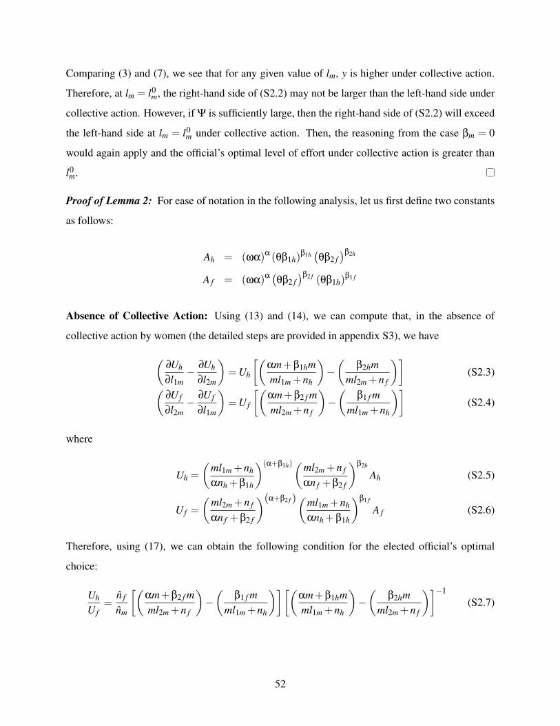
Comparing (3) and (7), we see that for any given value of lm, y is higher under collective action.

Therefore, at lm = l0m, the right-hand side of (S2.2) may not be larger than the left-hand side under

collective action. However, if Ψ is sufficiently large, then the right-hand side of (S2.2) will exceed

the left-hand side at lm = l0m under collective action. Then, the reasoning from the case βm = 0

would again apply and the official’s optimal level of effort under collective action is greater than

l0m.

Proof of Lemma 2: For ease of notation in the following analysis, let us first define two constants

as follows:

Ah = (ωα)α (θβ1h)β1h(θβ2 f

)β2h

A f = (ωα)α(θβ2 f

)β2 f (θβ1h)β1 f

Absence of Collective Action: Using (13) and (14), we can compute that, in the absence of

collective action by women (the detailed steps are provided in appendix S3), we have

(∂Uh

∂l1m− ∂Uh

∂l2m

)=Uh

[(αm+β1hmml1m +nh

)−(

β2hmml2m +n f

)](S2.3)(

∂U f

∂l2m−

∂U f

∂l1m

)=U f

[(αm+β2 f mml2m +n f

)−(

β1 f mml1m +nh

)](S2.4)

where

Uh =

(ml1m +nh

αnh +β1h

)(α+β1h)(

ml2m +n f

αn f +β2 f

)β2h

Ah (S2.5)

U f =

(ml2m +n f

αn f +β2 f

)(α+β2 f )(ml1m +nh

αnh +β1h

)β1 f

A f (S2.6)

Therefore, using (17), we can obtain the following condition for the elected official’s optimal

choice:

Uh

U f=

n f

nm

[(αm+β2 f mml2m +n f

)−(

β1 f mml1m +nh

)][(αm+β1hmml1m +nh

)−(

β2hmml2m +n f

)]−1

(S2.7)

52

We obtain, from (S2.5), (S2.6) and (S2.7),

Uh

U f=

(ml1m +nh

αnh +β1h

)(α+β1h−β1 f )(ml2m +n f

αn f +β2 f

)β2h−β2 f−α Ah

A f(S2.8)

Presence of Collective Action: Using (15) and (16), we can compute that, in the presence of

collective action (the detailed steps are provided in appendix S3), we have

(∂Uh

∂l1m− ∂Uh

∂l2m

)=Uh

[(αm+β1hmml1m +nh

)−(

β2hmml2m +n f

)](S2.9)(

∂U f

∂l2m−

∂U f

∂l1m

)=U f

[(αm+β2 f mml2m +n f

)−(

β1 f mml1m +nh

)](S2.10)

where

Uh =

(ml1m +nh

αnh +β1h

)(α+β1h)(

ml2m +n f

α+β2 f

)β2h

Ah (S2.11)

U f =

(ml2m +n f

α+β2 f

)(α+β2 f )(ml1m +nh

αnh +β1h

)β1 f

A f (S2.12)

Therefore, using (17), the optimal choice requires that

Uh

U f=

n f

nm

[(αm+β2 f mml2m +n f

)−(

β1 f mml1m +nh

)][(αm+β1hmml1m +nh

)−(

β2hmml2m +n f

)]−1

(S2.13)

We obtain, from (S2.11), (S2.12) and (S2.13),

Uh

U f=

(ml1m +nh

αnh +β1h

)(α+β1h−β1 f )(ml2m +n f

α+β2 f

)β2h−β2 f−α Ah

A f(S2.14)

Comparing (S2.8) and (S2.14), it is clear that, for given l1m and l2m and β2 f > β2h, the ratio of

utilities is smaller under collective action if n f > 1. Therefore, if l′1m and l′2m satisfies (S2.13) in

the absence of collective action, we have

Uh

U f<

n f

nm

[(αm+β2 f mml2m +n f

)−(

β1 f mml1m +nh

)][(αm+β1hmml1m +nh

)−(

β2hmml2m +n f

)]−1

(S2.15)

in the presence of collective action. The left-hand side of (S2.15) is increasing in l1m and decreasing

53

in l2m. The right-hand side of (S2.15) is decreasing in l2m and increasing in l1m. Therefore, if

l′′1m, l′′2m solves (S2.13) and l′′1m + l′′2m = l′1m + l′2m, then we must have l′2m > l′′2m and l′1m < l′′1m.

Lemma 3. Assume that the elected official maximises a weighted sum of utilities of the electorate,

applying the same weight to individuals of the same gender, and the total amount of the elected

official’s labour available for the two public goods is fixed. Assume also that men undertake

collective action in the provision of public good 1. Under Assumptions 2 and 3, if women organise

to take collective action in the provision of public good 2, the elected official shifts labour from

public good 1 to public good 2, compared to the situation where they do not.

Proof. We assume in the following that men undertake collective action in contributing to Pub-

lic Good 1. Following the reasoning in Section II, it can be shown that the utility levels of the

community members in the absence of collective action by women is given by

Uh (xh,y1,y2) =

(ml1m +nh

αnh +β1h

)α+β1h(

ml2m +n f

α+β2 f

)β2h

(ωα)α (θβ1h)β1h(θβ2 f

)β2h

U f(x f ,y1,y2

)=

(ml2m +n f

α+β2 f

)α+β2 f(

ml1m +nh

αnh +β1h

)β1 f

(ωα)α(θβ2 f

)β2 f (θβ1h)β1 f

and the utility levels of the community members in the presence of collective action by women is

given by

Uh (xh,y1,y2) =

(ml1m +nh

α+β1h

)α+β1h(

ml2m +n f

α+β2 f

)β2h

(ωα)α (θβ1h)β1h(θβ2 f

)β2h

U f(x f ,y1,y2

)=

(ml2m +n f

α+β2 f

)α+β2 f(

ml1m +nh

α+β1h

)β1 f

(ωα)α(θβ2 f

)β2 f (θβ1h)β1 f

Then, following the reasoning provided in the proof of Lemma 2, we can show that the elected

official’s optimal choice requires

Uh

U f=

(ml1m +nh

α+β1h

)(α+β1h−β1 f )(ml2m +n f

αn f +β2 f

)β2h−β2 f−α Ah

A f

if women do not undertake collecive action, and

Uh

U f=

(ml1m +nh

α+β1h

)(α+β1h−β1 f )(ml2m +n f

α+β2 f

)β2h−β2 f−α Ah

A f

54

if women do undertake collective action. Comparing the two equations, it is clear that, for given

l1m and l2m and β2 f > β2h, the ratio of utilities is smaller under collective action if n f > 1. Then,

following the reasoning in the proof of Lemma 2, we can show that if l′1m and l′2m satisfies (18) in

the absence of collective action, and l′′1m, l′′2m solves (18) in the presence of collective action, we

must have l′2m > l′′2m and l′1m < l′′1m.

Proof of Proposition 2: The first-order condition’s from the elected official’s optimisation prob-

lem can be written as follows:

(y2)β2m[αmω(xm)

αm−1 (y1)β1m−β1mmθ(xm)

αm (y1)β1m−1

]= Ψπ

′ (.)

[nh

dUh

dl1m+ n f

dU f

dl1m

](S2.16)

(y1)β1m[αmω(xm)

αm−1 (y2)β2m−β2mmθ(xm)

αm (y2)β2m−1

]= Ψπ

′ (.)

[nh

dUh

dl2m+ n f

dU f

dl2m

](S2.17)

β1mmθ(xm)αm (y1)

β1m−1 (y2)β2m−β2mmθ(xm)

αm (y1)β1m (y2)

β2m−1

= Ψπ′ (.)

[n f

(dU f

dl2m−

dU f

dl1m

)− nh

(dUh

dl1m− dUh

dl2m

)](S2.18)

Let us denote by l∗xm, l∗1m, l

∗2m, the elected official’s optimal choice in the absence of collective action

by women.

(i) Let us first consider the case where β1m = β2m = 0. It can be shown that, for any given

values of l1m, l2m, the terms dUhdl1m

and dU fdl1m

are higher when women undertake collective action as

compared to when they do not. Therefore, the right-hand side of (S2.16) is higher when women

undertake collective action (note that, under Assumption 4, the term π′ (.) is constant). Moreover,

if β1m = β2m = 0, then the expression on the left-hand side of (S2.16) is the same whether or

not women undertake collective action. It follows that at lxm = l∗xm, l1m = l∗1m, l2m = l∗2m, the left-

hand side of (S2.16) is smaller than the right-hand side when women undertake collective action.

Therefore, we must have either l1m > l∗1m or l2m > l∗2m (or both) when women undertake collective

action.

If β1m = β2m = 0, then the left-hand side of (S2.18) is equal to zero whether or not women

55

undertake collective action. If l1m > l∗1m and l2m ≤ l∗2m, then following the reasoning in the proof

of Lemma 2 (in the case that men do not undertake collective action) or Lemma 3 (in the case that

men do undertake collective action), the right hand-side of (S2.18) is greater than zero. Therefore,

we can rule out the possibility that the elected official’s optimal labour allocation involves l1m > l∗1m

and l2m≤ l∗2m when women undertake collective action. It follows that the elected official’s optimal

choice must involve l2m > l∗2m when women undertake collective action.

(ii) Next, let us consider the case where β1m,β2m > 0. Then, for any given values of lxm, l1m and

l2m, the expression on the left-hand side of (S2.16) is also higher when women undertake collective

action as compared to when they do not. However we can show that, at lxm = l∗xm, l1m = l∗1m, l2m =

l∗2m, for Ψ sufficiently large, the left-hand side of (S2.16) is, again, smaller than the right-hand side

when women undertake collective action. Therefore, we must have either l1m > l∗1m or l2m > l∗2m (or

both) when women undertake collective action. Similarly, if β1m,β2m > 0, the expression on the

left-hand side of (S2.18) is also higher when women undertake collective action. But, once again,

if l1m > l∗1m and l2m ≤ l∗2m, the expression on the right-hand of (S2.18) will exceed the left-hand

side for Ψ sufficiently large. It follows that, for Ψ sufficiently large, the elected official’s optimal

choice must involve l2m > l∗2m when women undertake collective action.

56

Appendix S3: Derivations used in Proof of Lemma 2

In this appendix, we show in detail the steps for deriving equations (S2.3)-(S2.4) and (S2.9)-

(S2.10). We make use of the following constants in computing the elected official’s marginal

utility of effort.

Ah = (ωα)α (θβ1h)β1h(θβ2 f

)β2h

A f = (ωα)α(θβ2 f

)β2 f (θβ1h)β1 f

Using (13) and (14), we find that, in the absence of collective action, we have

∂Uh

∂l1m=

(m

αnh +β1h

)(α+β1h)

(ml1m +nh

αnh +β1h

)(α+β1h−1)(ml2m +n f

αn f +β2 f

)β2h

Ah

∂U f

∂l1m=

(m

αnh +β1h

)(β1 f)(ml2m +n f

αn f +β2 f

)(α+β2 f )(ml1m +nh

αnh +β1h

)(β1 f−1)A f

∂Uh

∂l2m=

(m

αn f +β2 f

)(β2h)

(ml1m +nh

αnh +β1h

)(α+β1h)(

ml2m +n f

αn f +β2 f

)(β2h−1)

Ah

∂U f

∂l2m=

(m

αn f +β2 f

)(α+β2 f

)(ml2m +n f

αn f +β2 f

)(α+β2 f−1)(ml1m +nh

αnh +β1h

)β1 f

A f

Therefore,

(∂Uh

∂l1m− ∂Uh

∂l2m

)= Uh

[(αm+β1hmαnh +β1h

)(ml1m +nh

αnh +β1h

)−1

−(

β2hmαn f +β2 f

)(ml2m +n f

αn f +β2 f

)−1]

= Uh

[(αm+β1hmml1m +nh

)−(

β2hmml2m +n f

)]

Similarly, (∂U f

∂l2m−

∂U f

∂l1m

)=U f

[(αm+β2 f mml2m +n f

)−(

β1 f mml1m +nh

)]

57

Using (15) and (16), we find that, in the presence of collective action, we have

∂Uh

∂l1m=

(m

αnh +β1h

)(α+β1h)

(ml1m +nh

αnh +β1h

)(α+β1h−1)(ml2m +n f

α+β2 f

)β2h

Ah

∂U f

∂l1m=

(m

αnh +β1h

)(β1 f)(ml2m +n f

α+β2 f

)α+β2 f(

ml1m +nh

αnh +β1h

)(β1 f−1)A f

∂Uh

∂l2m=

(m

α+β2 f

)(β2h)

(ml1m +nh

αnh +β1h

)(α+β1h)(

ml2m +n f

α+β2 f

)(β2h−1)

Ah

∂U f

∂l2m=

(m

α+β2 f

)(α+β2 f

)(ml2m +n f

α+β2 f

)(α+β2 f−1)(ml1m +nh

αnh +β1h

)β1 f

A f

Therefore,

(∂Uh

∂l1m− ∂Uh

∂l2m

)= Uh

[(αm+β1hmαnh +β1h

)(ml1m +nh

αnh +β1h

)−1

−(

β2hmα+β2 f

)(ml2m +n f

α+β2 f

)−1]

= Uh

[(αm+β1hmml1m +nh

)−(

β2hmml2m +n f

)]

(∂U f

∂l2m−

∂U f

∂l1m

)= U f

[(αm+β2 f m

α+β2 f

)(ml2m +n f

α+β2 f

)−1

−(

β1 f mαnh +β1h

)(ml1m +nh

αnh +β1h

)−1]

= U f

[(αm+β2 f mml2m +n f

)−(

β1 f mml1m +nh

)]

58