Embed Size (px)
Citation preview

PTK: A PARALLEL TOOLKIT LIBRARY
by
Kirsten Ann Allison
A thesis
submitted in partial fulfillment
of the requirements for the degree of
Master of Science in Computer Science
Boise State University
March 2007

c© 2007Kirsten Ann Allison
ALL RIGHTS RESERVED
The thesis presented by Kirsten Ann Allison entitled PTK: A Parallel Toolkit Libraryis hereby approved.
Amit Jain, Advisor Date
John Griffin, Committee Member Date
Jyh-Haw Yeh, Committee Member Date
John R. Pelton, Graduate Dean Date

dedicated to my father
iv

ACKNOWLEDGEMENTS
This experience was possible because I have an incredible husband, Mark, and
boys, Connor and Teagan. They have sacrificed much in the last year and a half. My
parents have always told me that I can be anything I want to be. This has served
me well. My sister has been extremely encouraging and supportive. My friends have
helped me find brief moments of sanity, not to mention help with kids. It takes a
village to produce a thesis.
Many thanks go to Dr. Amit Jain for his teaching and patience. When I embarked
on this journey, I hadn’t written a line of code in eight years. I imagine some of my
questions were not particularly brilliant. He has a wonderful knack for knowing when
to help and when to send me away to figure it out on my own.
Thank you, also, to the Department of Computer Science for its support. When
Dr. Griffin called me in August 2006 to ask when I was planning on getting my
paperwork in to the department, my planned experiment of taking one class turned
into being a full time student with a teaching assistantship. Little did I know what I
was getting into. Dr. Teresa Cole has been an immense help to my success as a TA
and student.
Thank you to Conrad Kennington and Luke Hindman. The talks on the way to
get coffee often helped me clarify an idea, and provided fuel for the next round.
This material is based upon work supported by the National Science Foundation
under Grant No. 0321233. Any opinions, findings, and conclusions or recommen-
dations expressed in this material are those of the author(s) and do not necessarily
reflect the views of the National Science Foundation.
v
AUTOBIOGRAPHICAL SKETCH
Kirsten Allison took her first programming class in fourth grade. She has always
loved solving problems.
She received her degree in Computer Science from the University of Minnesota.
Upon graduation, she moved to Oregon to work for Tektronix. Her Tek years were
spent in a cubical writing code. On deciding that she’d like to get out of that cube
other than to go to meetings, she went to work for Integrated Measurement Systems
as an Applications Engineer. She spent much of her time in Asia, helping customize
systems to meet users’ needs. It was nice to get out of that cubicle, but airplanes
become very small when you’ve been on them for 20 hours, and it became time for
another change.
The next adventure was on to a much greater challenge. Kirsten chose to take
a break from “work” and be a full-time parent. This was in the wake of significant
research on brain development in the first three years of life, and the importance
of providing a “proper environment” for that development, and a cultural shift of
women heading home. The impact of these cultural changes is a thesis in itself.
A number of years at home made it clear that it was time to go back to work.
Going back to school seemed a logical step along that path. Her Boise State experience
has been a challenge and a joy. She believes it will serve her well in venturing back
out into “the real world.”
vi

ABSTRACT
The High Performance Computing(HPC) market has made a significant shift from
large, monolithic, specialized systems to networked clusters of workstations. This has
been precipitated by the continuing upward movement of the price/performance ratio
of commodity computing hardware. The fast growth of this market has presented a
challenge to the open source community. Software has not necessarily kept up with
the growth.
The Parallel Toolkit Library provides support for common design patterns used
throughout parallel programs. It includes both PVM and MPI versions. The examples
given help users understand how to use the library functions.
The data sharing patterns of gather, scatter, and all to all are fully supported.
They allow users the flexibility of having odd amounts of data that are not evenly
divisible by the number of processes. The two-dimensional versions allow the user to
share “ragged” arrays of data. These elements are not provided by PVM or MPI.
The file merging functionality automates a common cluster task.
The workpools remove a significant layer of detail from writing workpool code.
The user of the workpool needs to provide the library with functions for processing
tasks and results. The library takes care of sending and receiving tasks and results.
Most importantly it handles termination detection, which can be quite cumbersome
to design and write.
The testing and benchmarking results are consistent with expectations. The li-
brary does not add a significant amount of overhead. In some cases, it may be more ef-
ficient than code that users would write, because time may not be taken in non-library
vii

code to incorporate some efficiencies that are part of the toolkit library. The library
and example code is available at http://cs.boisestate.edu/~amit/research/ptk.
Libraries such as the toolkit are critical to making clusters easier to write programs
for. The toolkit removes a layer of detail for the programmer to need to understand.
This will make writing parallel programs easier and faster. The toolkit also provides
a tested set of features that will make users’ programs more robust.
viii
TABLE OF CONTENTS
LIST OF TABLES . . . . . . . . . . . . . . . . . . . . . . . . . . . . . . . xiv
LIST OF FIGURES . . . . . . . . . . . . . . . . . . . . . . . . . . . . . . xv
1 INTRODUCTION . . . . . . . . . . . . . . . . . . . . . . . . . . . . . 1
1.1 Problem Statement . . . . . . . . . . . . . . . . . . . . . . . . . . . . 1
1.2 Prior Research . . . . . . . . . . . . . . . . . . . . . . . . . . . . . . 3
1.3 General Thoughts on Library Development . . . . . . . . . . . . . . . 4
1.3.1 Adequate Functionality Versus Ease of Use . . . . . . . . . . . 4
1.3.2 Memory Allocation - Where Should It Happen? . . . . . . . . 4
1.4 Terminology . . . . . . . . . . . . . . . . . . . . . . . . . . . . . . . . 4
1.4.1 Process Groups . . . . . . . . . . . . . . . . . . . . . . . . . . 4
1.4.2 Blocking Versus Non-Blocking Sends and Receives . . . . . . . 5
2 TOOLKIT IMPLEMENTATION . . . . . . . . . . . . . . . . . . . . 6
2.1 Some General Differences Between PVM and MPI . . . . . . . . . . . 6
2.1.1 Groups . . . . . . . . . . . . . . . . . . . . . . . . . . . . . . . 6
2.1.2 Message Ordering . . . . . . . . . . . . . . . . . . . . . . . . . 8
2.2 Common Toolkit Parameters and Elements . . . . . . . . . . . . . . . 8
2.2.1 Verbose . . . . . . . . . . . . . . . . . . . . . . . . . . . . . . 8
2.2.2 PVM Datatypes . . . . . . . . . . . . . . . . . . . . . . . . . . 9
2.2.3 MPI Datatypes . . . . . . . . . . . . . . . . . . . . . . . . . . 9
ix
2.3 ptk init . . . . . . . . . . . . . . . . . . . . . . . . . . . . . . . . . . 10
2.3.1 PVM Usage . . . . . . . . . . . . . . . . . . . . . . . . . . . . 11
2.3.2 MPI Usage . . . . . . . . . . . . . . . . . . . . . . . . . . . . 11
2.4 ptk scatter1d . . . . . . . . . . . . . . . . . . . . . . . . . . . . . . . 12
2.4.1 Usage . . . . . . . . . . . . . . . . . . . . . . . . . . . . . . . 13
2.5 ptk scatter2d . . . . . . . . . . . . . . . . . . . . . . . . . . . . . . . 14
2.5.1 Usage . . . . . . . . . . . . . . . . . . . . . . . . . . . . . . . 16
2.6 ptk gather1d . . . . . . . . . . . . . . . . . . . . . . . . . . . . . . . 16
2.6.1 Usage . . . . . . . . . . . . . . . . . . . . . . . . . . . . . . . 17
2.7 ptk gather2d . . . . . . . . . . . . . . . . . . . . . . . . . . . . . . . 17
2.7.1 Usage . . . . . . . . . . . . . . . . . . . . . . . . . . . . . . . 19
2.8 ptk alltoall1d . . . . . . . . . . . . . . . . . . . . . . . . . . . . . . . 20
2.8.1 Usage . . . . . . . . . . . . . . . . . . . . . . . . . . . . . . . 21
2.9 ptk alltoall2d . . . . . . . . . . . . . . . . . . . . . . . . . . . . . . . 21
2.9.1 Usage . . . . . . . . . . . . . . . . . . . . . . . . . . . . . . . 24
2.10 ptk mcast . . . . . . . . . . . . . . . . . . . . . . . . . . . . . . . . . 24
2.10.1 PVM Usage . . . . . . . . . . . . . . . . . . . . . . . . . . . . 25
2.10.2 MPI Usage . . . . . . . . . . . . . . . . . . . . . . . . . . . . 25
2.11 ptk filemerge . . . . . . . . . . . . . . . . . . . . . . . . . . . . . . . 26
2.11.1 Usage . . . . . . . . . . . . . . . . . . . . . . . . . . . . . . . 26
2.12 ptk central workpool . . . . . . . . . . . . . . . . . . . . . . . . . . . 27
2.12.1 Usage . . . . . . . . . . . . . . . . . . . . . . . . . . . . . . . 28
2.12.2 Implementation Discussion . . . . . . . . . . . . . . . . . . . . 31
2.13 ptk distributed workpool . . . . . . . . . . . . . . . . . . . . . . . . . 35
x
2.13.1 Usage . . . . . . . . . . . . . . . . . . . . . . . . . . . . . . . 37
2.13.2 Implementation Discussion . . . . . . . . . . . . . . . . . . . . 43
2.14 ptk wtime . . . . . . . . . . . . . . . . . . . . . . . . . . . . . . . . . 49
2.15 ptk exit . . . . . . . . . . . . . . . . . . . . . . . . . . . . . . . . . . 50
2.15.1 PVM Usage . . . . . . . . . . . . . . . . . . . . . . . . . . . . 50
2.15.2 MPI Usage . . . . . . . . . . . . . . . . . . . . . . . . . . . . 51
2.16 Miscellaneous Files Used By the Toolkit . . . . . . . . . . . . . . . . 51
2.16.1 ptk array . . . . . . . . . . . . . . . . . . . . . . . . . . . . . 51
2.16.2 ptk pvmgs . . . . . . . . . . . . . . . . . . . . . . . . . . . . . 51
3 USING THE TOOLKIT: SOME EXAMPLES . . . . . . . . . . . . 52
3.1 Gather and Scatter . . . . . . . . . . . . . . . . . . . . . . . . . . . . 52
3.1.1 A Simple One-Dimensional Gather . . . . . . . . . . . . . . . 52
3.1.2 A One-Dimensional Scatter Example . . . . . . . . . . . . . . 55
3.1.3 Bucketsort Using Two-Dimensional Scatter . . . . . . . . . . . 55
3.2 All to All . . . . . . . . . . . . . . . . . . . . . . . . . . . . . . . . . 56
3.2.1 A Simple All to All . . . . . . . . . . . . . . . . . . . . . . . . 56
3.2.2 Bucketsort Using All to All . . . . . . . . . . . . . . . . . . . 56
3.3 Merging Files From Across a Cluster . . . . . . . . . . . . . . . . . . 57
3.4 The Workpools . . . . . . . . . . . . . . . . . . . . . . . . . . . . . . 58
3.4.1 Choosing the Appropriate Workpool . . . . . . . . . . . . . . 58
3.4.2 Centralized Workpool . . . . . . . . . . . . . . . . . . . . . . . 60
3.4.3 Distributed Workpool . . . . . . . . . . . . . . . . . . . . . . 66
4 TESTING AND BENCHMARKING . . . . . . . . . . . . . . . . . 71
xi
5 CONCLUSIONS . . . . . . . . . . . . . . . . . . . . . . . . . . . . . . 78
5.1 Library Support for Common Parallel Design Patterns . . . . . . . . 78
5.2 General Observations and Reflections on Decisions Made . . . . . . . 79
5.3 Potential Further Work . . . . . . . . . . . . . . . . . . . . . . . . . . 79
5.3.1 Centralized Workpool Queue . . . . . . . . . . . . . . . . . . . 79
5.3.2 Multi-threading . . . . . . . . . . . . . . . . . . . . . . . . . . 79
5.3.3 C++ . . . . . . . . . . . . . . . . . . . . . . . . . . . . . . . . 80
REFERENCES . . . . . . . . . . . . . . . . . . . . . . . . . . . . . . . . . 81
APPENDIX A SHORTEST PATHS CODE . . . . . . . . . . . . . . . 83
A.1 Shortest Paths Centralized - Simple . . . . . . . . . . . . . . . . . . . 83
A.1.1 Processing tasks . . . . . . . . . . . . . . . . . . . . . . . . . . 83
A.1.2 Processing results . . . . . . . . . . . . . . . . . . . . . . . . . 84
A.2 Shortest Paths Centralized - More Efficient . . . . . . . . . . . . . . . 86
A.2.1 Processing tasks . . . . . . . . . . . . . . . . . . . . . . . . . . 86
A.2.2 Processing results . . . . . . . . . . . . . . . . . . . . . . . . . 88
A.3 Shortest Paths Distributed - Simple . . . . . . . . . . . . . . . . . . . 91
A.3.1 Processing tasks . . . . . . . . . . . . . . . . . . . . . . . . . . 91
A.3.2 Processing results . . . . . . . . . . . . . . . . . . . . . . . . . 93
A.4 Shortest Paths Distributed - More Efficient . . . . . . . . . . . . . . . 94
A.4.1 Processing tasks . . . . . . . . . . . . . . . . . . . . . . . . . . 94
A.4.2 Processing results . . . . . . . . . . . . . . . . . . . . . . . . . 97
APPENDIX B TIMING DATA . . . . . . . . . . . . . . . . . . . . . . 98
xii

APPENDIX C INSTALLING THE PTK LIBRARY . . . . . . . . . 101
APPENDIX D BOISE STATE COMPUTER SCIENCE DEPARTMENTCLUSTERS . . . . . . . . . . . . . . . . . . . . . . . . . . . . . . . . . 102
D.1 Onyx . . . . . . . . . . . . . . . . . . . . . . . . . . . . . . . . . . . . 102
D.2 Beowulf . . . . . . . . . . . . . . . . . . . . . . . . . . . . . . . . . . 102
xiii
LIST OF TABLES
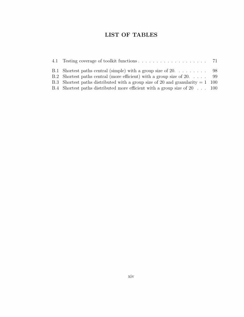
4.1 Testing coverage of toolkit functions . . . . . . . . . . . . . . . . . . . 71
B.1 Shortest paths central (simple) with a group size of 20. . . . . . . . . 98B.2 Shortest paths central (more efficient) with a group size of 20. . . . . 99B.3 Shortest paths distributed with a group size of 20 and granularity = 1 100B.4 Shortest paths distributed more efficient with a group size of 20 . . . 100
xiv
LIST OF FIGURES
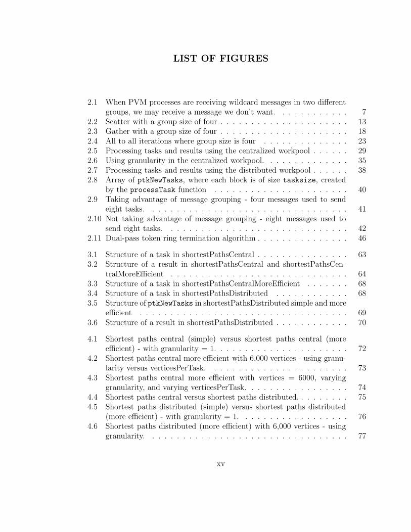
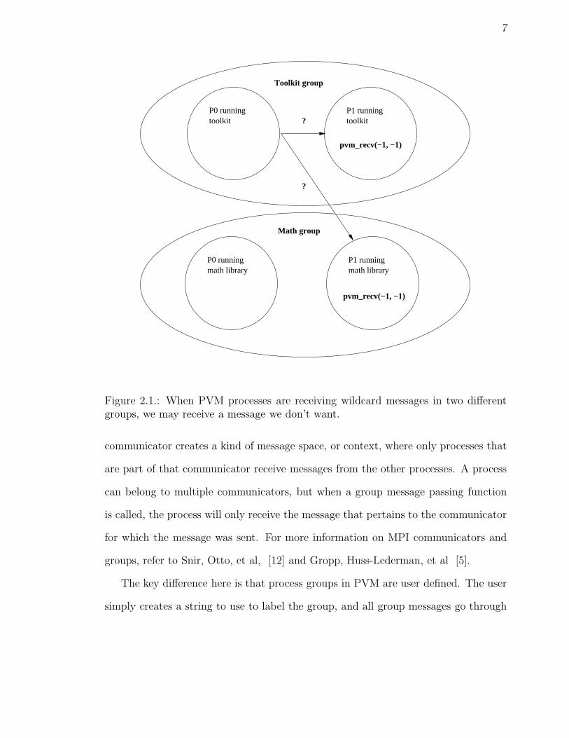
2.1 When PVM processes are receiving wildcard messages in two differentgroups, we may receive a message we don’t want. . . . . . . . . . . . 7
2.2 Scatter with a group size of four . . . . . . . . . . . . . . . . . . . . . 132.3 Gather with a group size of four . . . . . . . . . . . . . . . . . . . . . 182.4 All to all iterations where group size is four . . . . . . . . . . . . . . 232.5 Processing tasks and results using the centralized workpool . . . . . . 292.6 Using granularity in the centralized workpool. . . . . . . . . . . . . . 352.7 Processing tasks and results using the distributed workpool . . . . . . 382.8 Array of ptkNewTasks, where each block is of size tasksize, created
by the processTask function . . . . . . . . . . . . . . . . . . . . . . 402.9 Taking advantage of message grouping - four messages used to send
eight tasks. . . . . . . . . . . . . . . . . . . . . . . . . . . . . . . . . 412.10 Not taking advantage of message grouping - eight messages used to
send eight tasks. . . . . . . . . . . . . . . . . . . . . . . . . . . . . . 422.11 Dual-pass token ring termination algorithm . . . . . . . . . . . . . . . 46
3.1 Structure of a task in shortestPathsCentral . . . . . . . . . . . . . . . 633.2 Structure of a result in shortestPathsCentral and shortestPathsCen-
tralMoreEfficient . . . . . . . . . . . . . . . . . . . . . . . . . . . . . 643.3 Structure of a task in shortestPathsCentralMoreEfficient . . . . . . . 683.4 Structure of a task in shortestPathsDistributed . . . . . . . . . . . . 683.5 Structure of ptkNewTasks in shortestPathsDistributed simple and more
efficient . . . . . . . . . . . . . . . . . . . . . . . . . . . . . . . . . . 693.6 Structure of a result in shortestPathsDistributed . . . . . . . . . . . . 70
4.1 Shortest paths central (simple) versus shortest paths central (moreefficient) - with granularity = 1. . . . . . . . . . . . . . . . . . . . . . 72
4.2 Shortest paths central more efficient with 6,000 vertices - using granu-larity versus verticesPerTask. . . . . . . . . . . . . . . . . . . . . . . 73
4.3 Shortest paths central more efficient with vertices = 6000, varyinggranularity, and varying verticesPerTask. . . . . . . . . . . . . . . . . 74
4.4 Shortest paths central versus shortest paths distributed. . . . . . . . . 754.5 Shortest paths distributed (simple) versus shortest paths distributed
(more efficient) - with granularity = 1. . . . . . . . . . . . . . . . . . 764.6 Shortest paths distributed (more efficient) with 6,000 vertices - using
granularity. . . . . . . . . . . . . . . . . . . . . . . . . . . . . . . . . 77
xv

4.7 Shortest paths distributed - condensed messaging affects performance. 77
xvi
1
Chapter 1
INTRODUCTION
1.1 Problem Statement
The dominant supercomputing platform is moving from large monolithic machines to
networked clusters of workstations. Continuing improvement in the price/performance
ratio of commodity computing hardware drives this change. The software written for
these clusters uses standardized message passing libraries. The two libraries most
commonly used are: PVM (Parallel Virtual Machine) [10] and MPI (Message Pass-
ing Interface) [7]. The increased availability and cost effectiveness of clusters has
increased the need for effective parallel programming tools. PVM and MPI are useful
libraries, but they are missing several elements. There are several common design
patterns, or tasks, that one wishes to perform in parallel programs, but these tasks
must be implemented from scratch every time a parallel program is written. These
tasks are strong candidates for inclusion in the Parallel Toolkit.
Gropp, Lusk, and Skjellum [6] make an excellent argument for the need for parallel
libraries:
“Software libraries offer several advantages:
• they ensure consistency in program correctness,
• they help guarantee a high-quality implementation,
• they hide distracting details and complexities associated with state-of-the-art implementations, and
2
• they minimize repetitive effort or haphazard results.”
Prior to beginning work on the toolkit, my parallel programming experience was
limited to my Parallel Computing course. In thinking about what should be included
in the toolkit, I relied heavily on Dr. Amit Jain to act as my “customer,” and provide
a list of requirements. The common design patterns that the toolkit needed to support
were:
• a centralized workpool that manages communication between a coordinating
node and worker nodes,
• a distributed workpool that manages communication between workers and han-
dles termination,
• all to all data sharing, where each node sends a subset of a collection of data to
each other node,
• a gather function, where a root node collects data from each node,
• a scatter function, where a root node sends a subset of a collection of data to
each other node,
• a multicast function, where a sending node sends a collection of data to each
other node, in its entirety,
• a filemerge function that collects files from all nodes in a group, and condenses
them into one file at a root node.
3
1.2 Prior Research
There is much to be found in the way of parallel libraries and applications. These
include copious math libraries, applications for doing computational chemistry and
biology, oceanic and atmospheric modeling, applications for building clusters, and
system administration tools. The applications tend to be very domain specific, but
not very useful for more general purpose computing. The Argonne National Lab’s
Mathematics and Computer Science Division maintains a list of their current software
projects at http://www-new.mcs.anl.gov/new/software.php, and a list of libraries
based on MPI at http://www-unix.mcs.anl.gov/mpi/libraries.html. There ap-
pears to be nothing there or on the web that is similar to the Parallel Toolkit.
A paper [11] was presented at the Midwest Instructional Computing Symposium in
2003 that documented the implementation of a “Hybrid Process Farm/Work Pool”.
The concept is similar to my workpool implementation. The code is not available
online. I have verified with the advisor of the paper that there is not an open source
version of this code available (see [8]). The code was implemented as part of a project
that has since been turned over to Sun Microsystems.
There is a graduate student in Germany who has implemented a workpool skeleton
in Eden, which is a parallel version of Haskell [9]. Most work on parallel skeletons is
associated with functional programming languages. Although there are some charac-
teristics of functional programming languages that make them useful for paralleliza-
tion, they are not mainstream development tools. Most parallel programming is done
in C and C++, so these skeletons cannot be viewed as pertinent to the discussion of
the parallel toolkit.
4
1.3 General Thoughts on Library Development
1.3.1 Adequate Functionality Versus Ease of Use
There were many times in the process of defining what a function should do, when the
question came up of “What if we added <fill in favorite extra bell or whistle here>?”
This then prompted discussion of how many parameters would need to be added to
make it work. Sometimes functionality was abandoned because it would have made
the function so complicated to use that no one would wanted to use it. Although
this may mean that the toolkit doesn’t solve every problem, it solves most of them
without an insurmountable learning curve.
1.3.2 Memory Allocation - Where Should It Happen?
One of the issues that came up is where to allocate memory for various data structures,
mainly arrays where data is filled in by the toolkit. There is a balance between
wanting the toolkit to do as much for the user as possible, while being as transparent
as possible at the same time. It seemed inconsistent and awkward to have the toolkit
allocate memory, and then expect the user to free it when done using the data. I
made the decision that wherever possible, the user should allocate and free memory.
Wherever possible, the toolkit allocates and frees memory within its own functions.
1.4 Terminology
1.4.1 Process Groups
A process group can be thought of as a ring, with each process having neighbors to its
right and left. The process group contains N processes. If we number the processes
5
from 0 to N − 1, then the right neighbor of process i is the process i + 1, and the
neighbor to the left of process i is the process i− 1. The left neighbor of process 0 is
process N − 1, and the right neighbor of process N − 1 is process 0.
1.4.2 Blocking Versus Non-Blocking Sends and Receives
When making a call to a blocking send, the process does not continue until the
message sent has been received. Likewise, in a blocking receive, the process does not
continue until there is a message available. In a non-blocking send or receive, control
returns immediately to the calling function. How this happens is different in PVM
and MPI, because they handle buffering differently. For a more extensive discussion,
see Wilkinson and Allen [13].
6
Chapter 2
TOOLKIT IMPLEMENTATION
2.1 Some General Differences Between PVM and MPI
2.1.1 Groups
One of the main differences between PVM and MPI is how they handle group com-
munication. PVM uses a centralized group server to differentiate process groups.
When a user wants to create a group in PVM, the pvm joingroup function is called,
which invokes the PVM group server. The group is defined by its name, which is
a simple string. This string is passed to the group functions and the functions are
only performed on members of the group. This is a very simplistic approach. It
becomes problematic when processes are doing “wildcard” receives. In a wildcard
receive, any receiver is looking for any type of message from any sender, which is
exactly what the toolkit does in the workpools. In that case, it is possible for the
toolkit functions to receive messages from other libraries or programs, or vice versa
(see Figure 2.1). This is not a limitation of the toolkit, but of PVM. Dongarra, Geist,
et al [3], present a proposal for adding static groups and contexts to PVM, but it has
not been implemented.
MPI, on the other hand, has a more sophisticated way of dealing with groups.
MPI uses “communicators” and groups to manage communication. These were in-
cluded in the MPI specification explicitly to support library development. An MPI
7
P0 runningtoolkit
P0 runningmath library
P1 runningtoolkit
P1 runningmath library
Math group
Toolkit group
?
?
pvm_recv(−1, −1)
pvm_recv(−1, −1)
Figure 2.1.: When PVM processes are receiving wildcard messages in two differentgroups, we may receive a message we don’t want.
communicator creates a kind of message space, or context, where only processes that
are part of that communicator receive messages from the other processes. A process
can belong to multiple communicators, but when a group message passing function
is called, the process will only receive the message that pertains to the communicator
for which the message was sent. For more information on MPI communicators and
groups, refer to Snir, Otto, et al, [12] and Gropp, Huss-Lederman, et al [5].
The key difference here is that process groups in PVM are user defined. The user
simply creates a string to use to label the group, and all group messages go through
8
a centralized group server. In MPI, the communicator is created by the system. This
allows point-to-point communication in MPI groups, without having to go through a
centralized group server. Needless to say, this eliminates a bottleneck in sending and
receiving group messages.
Another key difference between PVM and MPI groups is that PVM groups are
dynamic, that is, processes may join or leave a group at any time. This may lead
to race conditions if the programmer is not careful about how this is handled. MPI
groups are static. They are created and destroyed as whole groups.
2.1.2 Message Ordering
Message ordering is handled differently between PVM and MPI. PVM guarantees
message ordering. This means that if P0 sends Message A to P1, and then sends
Message B to P1, we can rely on Message A being received by P1 before Message B.
MPI does not give us this guarantee. In the collective data moving operations this is
not critical. It does becomes an issue in the workpools, where there are completely
asynchronous communication patterns.
2.2 Common Toolkit Parameters and Elements
2.2.1 Verbose
The verbose parameter specifies how much information the toolkit will provide about
its inner workings. Passing a verbose value of 0 will turn off output from the toolkit.
Note that the toolkit will still output error messages. Passing a verbose value of 1
will produce output from the toolkit. The output is particularly useful when trying
to debug a program that uses one of the workpools.
9
2.2.2 PVM Datatypes
The datatypes supported in the PVM version of the toolkit are defined as follows:
#define PTK_CHAR PVM_CHAR
#define PTK_SIGNED_CHAR PVM_SIGNED_CHAR
#define PTK_UNSIGNED_CHAR PVM_UNSIGNED_CHAR
#define PTK_BYTE PVM_BYTE
#define PTK_WCHAR PVM_WCHAR
#define PTK_SHORT PVM_SHORT
#define PTK_UNSIGNED_SHORT PVM_UNSIGNED_SHORT
#define PTK_INT PVM_INT
#define PTK_UNSIGNED PVM_UNSIGNED
#define PTK_LONG PVM_LONG
#define PTK_UNSIGNED_LONG PVM_UNSIGNED_LONG
#define PTK_FLOAT PVM_FLOAT
#define PTK_DOUBLE PVM_DOUBLE
#define PTK_LONG_DOUBLE PVM_LONG_DOUBLE
#define PTK_LONG_LONG_INT PVM_LONG_LONG_INT
#define PTK_UNSIGNED_LONG_LONG PVM_UNSIGNED_LONG_LONG
#define PTK_LONG_LONG PVM_LONG_LONG
#define PTK_PACKED PVM_PACKED
#define PTK_LB PVM_LB
#define PTK_UB PVM_UB
Note that although the code has been written as independently as possible of the
type of data, it has not been tested with all of the above datatypes.
2.2.3 MPI Datatypes
The datatypes supported in the MPI version of the toolkit are defined as follows:
#define PTK_CHAR MPI_CHAR
#define PTK_SIGNED_CHAR MPI_SIGNED_CHAR
#define PTK_UNSIGNED_CHAR MPI_UNSIGNED_CHAR
#define PTK_BYTE MPI_BYTE

10
#define PTK_WCHAR MPI_WCHAR
#define PTK_SHORT MPI_SHORT
#define PTK_UNSIGNED_SHORT MPI_UNSIGNED_SHORT
#define PTK_INT MPI_INT
#define PTK_UNSIGNED MPI_UNSIGNED
#define PTK_LONG MPI_LONG
#define PTK_UNSIGNED_LONG MPI_UNSIGNED_LONG
#define PTK_FLOAT MPI_FLOAT
#define PTK_DOUBLE MPI_DOUBLE
#define PTK_LONG_DOUBLE MPI_LONG_DOUBLE
#define PTK_LONG_LONG_INT MPI_LONG_LONG_INT
#define PTK_UNSIGNED_LONG_LONG MPI_UNSIGNED_LONG_LONG
#define PTK_LONG_LONG MPI_LONG_LONG
#define PTK_PACKED MPI_PACKED
#define PTK_LB MPI_LB
#define PTK_UB MPI_UB
Note that although the code has been written as independently as possible of the
type of data, it has not been tested with all of the above datatypes.
2.3 ptk init
int
ptk_init(int argc,
char **argv)
IN int argc The argc value equal to the value passed in to the
calling program.
IN char **argv The argv value equal to the value passed in to the
calling program.

11
2.3.1 PVM Usage
This is a basic function designed to provide the calling function with information
about the processing environment. The global variable gsize is assigned a value by
making a call to the pvm siblings function. This size is the number of processes that
were spawned together. The me global variable is assigned a value by making a call
to pvm joingroup and is the group instance number, or rank, of the process. These
instance numbers range from 0 to gsize - 1, and are unique, i.e., no two processes
can have the same instance number. The instance numbers are also contiguous.
The global array of task ids, tids is also populated. These are the task ids as
defined by the PVM group server. They are acquired by ptk init using the function
pvm gettid. Note that the order of tids in this array may be different than the array
that one would get by filling in the tids array with a call to pvm siblings(). The
ptk init function calls pvm joingroup. This invokes the PVM group server, which
creates a new internal array of task IDs. This array is filled in differently than the
task ID array created when the PVM processes are spawned. Among other things, the
PVM group server ensures that the task ID array is contiguous. This is an important
distinction. Users of the library should make sure that they are using an array of task
ids filled in by ptk init to ensure consistency.
2.3.2 MPI Usage
The argc and argv parameters should be self explanatory. They are used in a call
to MPI Init to pass parameters to all the processes. The gsize global variable is
given a value by calling MPI Comm size, and will be equivalent to all the processes
in PTK WORLD. PTK WORLD is an MPI Comm. An MPI Comm is a communi-
cator. For more discussion of communicators, refer to [6]. This function creates the
12
PTK WORLD from the MPI COMM WORLD. The me global variable is assigned a
value with a call to MPI Comm rank, and is the rank of the process in the group.
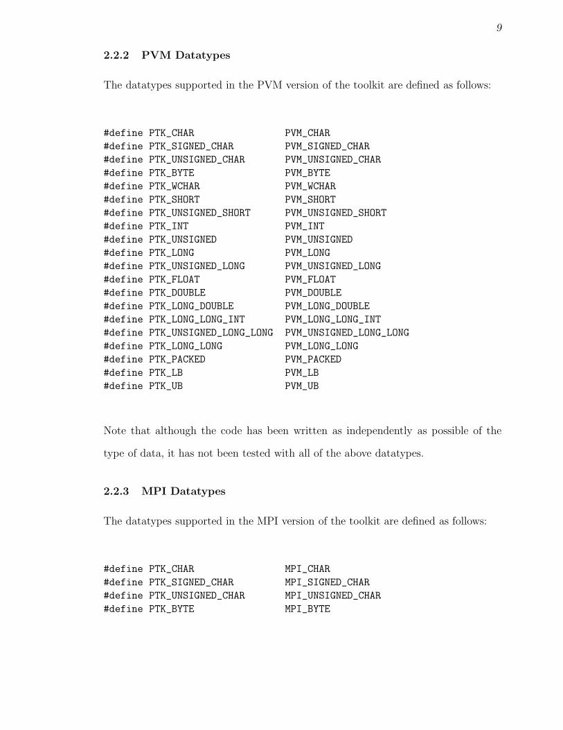
2.4 ptk scatter1d
int
ptk_scatter1D(void *sendbuf,
int sendcount,
int lastcount,
void *recvbuf,
int datatype,
int root,
int verbose)
IN void *sendbuf A one-dimensional array of any type of data, filled
in by the calling function at PTK ROOT.
IN int sendcount The number of elements to send to processes 0
through gsize - 2.
IN int lastcount The number of elements to send to process gsize
- 1.
OUT void *recvbuf A one-dimensional array of data, available at all
the processes after the call to ptk scatter1d. The
number of elements in the array at each process
is sendcount, with the exception of the last pro-
cess (process with the instance or rank equal to
gsize - 1). The size of the array is sendcount (or
lastcount) * datasize.
13
Data at the root node
... ... ... ...
? ? ? ?
P0 P1 P2 P3
0 sendcount- 1
sendcount
(send
count∗ 2)
- 1
sendcount∗ 2
(send
count∗ 3)
- 1
sendcount∗ 3
(send
count∗ 3)
+ last
count- 1
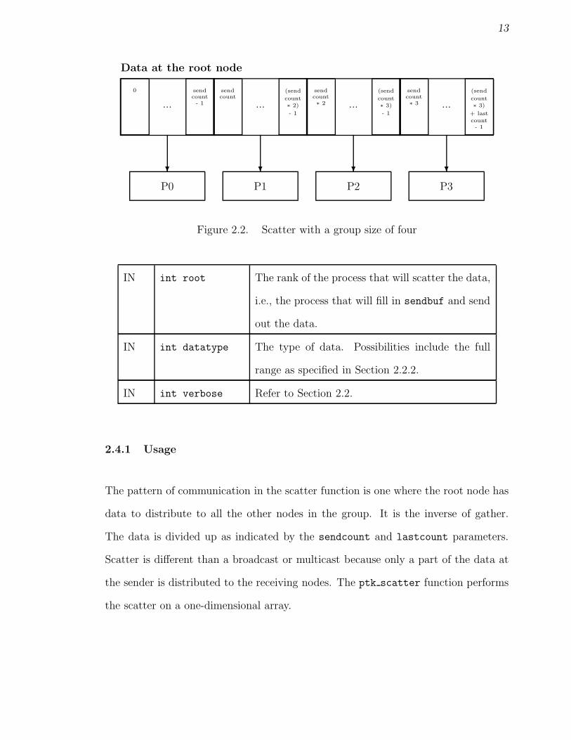
Figure 2.2. Scatter with a group size of four
IN int root The rank of the process that will scatter the data,
i.e., the process that will fill in sendbuf and send
out the data.
IN int datatype The type of data. Possibilities include the full
range as specified in Section 2.2.2.
IN int verbose Refer to Section 2.2.
2.4.1 Usage
The pattern of communication in the scatter function is one where the root node has
data to distribute to all the other nodes in the group. It is the inverse of gather.
The data is divided up as indicated by the sendcount and lastcount parameters.
Scatter is different than a broadcast or multicast because only a part of the data at
the sender is distributed to the receiving nodes. The ptk scatter function performs
the scatter on a one-dimensional array.
14
There is a pvm scatter function available. It has a significant limitation in that it
requires the size of the send buffer to be evenly divisible by the number of processes.
While this limitation must make its implementation much simpler, in reality there are
situations where there is an odd amount of data. The ptk scatter function supports
having an array with a size not evenly divisible by the group size.
In the first version of this function, I implemented it so that the user passed in the
array to scatter, and the size of the array. The toolkit then sent a chunk of data to
each process that was the size of the array divided (as evenly as possible) by the group
size, with the leftover going to the last process. I then ran into a situation in one
of the examples where I wanted to be able to divide the data up into “chunks.” For
example, if I have 3 processes, and an array with 100 elements, I wanted 30 elements
to go to the first two processes, and 40 to go to the last process.
Adding this functionality necessitated the use of an extra parameter. That means
there is more the user needs to understand, but I believe the trade off is justified
because the functionality is needed.
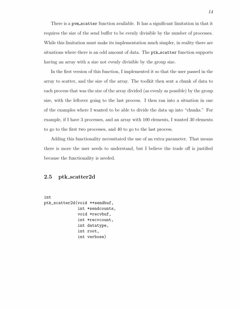
2.5 ptk scatter2d
int
ptk_scatter2d(void **sendbuf,
int *sendcounts,
void *recvbuf,
int *recvcount,
int datatype,
int root,
int verbose)

15
IN void **sendbuf A two-dimensional array of any type of data, filled
in by the calling function at PTK ROOT.
IN int
*sendcounts
Each entry in the sendcounts array is equivalent
to the number of elements to send to the corre-
sponding process. For example, if sendcounts[3]
is equal to 32, then 32 elements of type datatype
will be sent to process 3.
OUT void *recvbuf A one-dimensional array of data, available at all
the processes after the call to ptk scatter2d. The
number of elements in the array at each process
is sendcounts[myginst]. The size of each row is
defined in sendcounts.
OUT int *recvcount A reference to an integer. This value is filled in
and is equivalent to the number of elements put
in the recvbuf array.
IN int root The rank of the process that will scatter the data,
i.e., the process that will fill in sendbuf and send
out the data.
IN int datatype The type of data. Possibilities include the full
range as specified in Section 2.2.2.
IN int verbose Refer to Section 2.2.
16
2.5.1 Usage
In this version of scatter, the root sends a varying amount of data to each process.
The communication pattern is the same as that described for a 1-dimensional scatter.
The array to be sent is a two-dimensional array. The number of rows in the array
must be equal to the number of processes in the group. Another array is passed in,
called sendcounts. This array specifies how many elements there are in each row of
the sendbuf.
Another one-dimensional array, the recvbuf is also passed in. The toolkit al-
locates memory for this array as data is received. There is no way for the calling
function to allocate this memory, because it does not necessarily know how big the
array will be. This array is populated by the data in the corresponding row of the
two-dimensional send buffer. For example, P3 will have a recvbuf full of the data in
row sendbuf[3] at the root.
The calling function must specify the datatype of the send and receive buffers.
This information is used to select the appropriate pvm pack and unpack functions,
and to determine the size of the data.
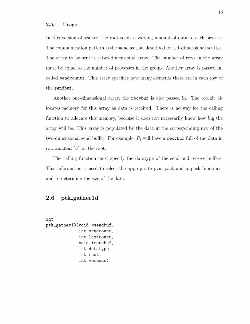
2.6 ptk gather1d
int
ptk_gather1D(void *sendbuf,
int sendcount,
int lastcount,
void *recvbuf,
int datatype,
int root,
int verbose)
17
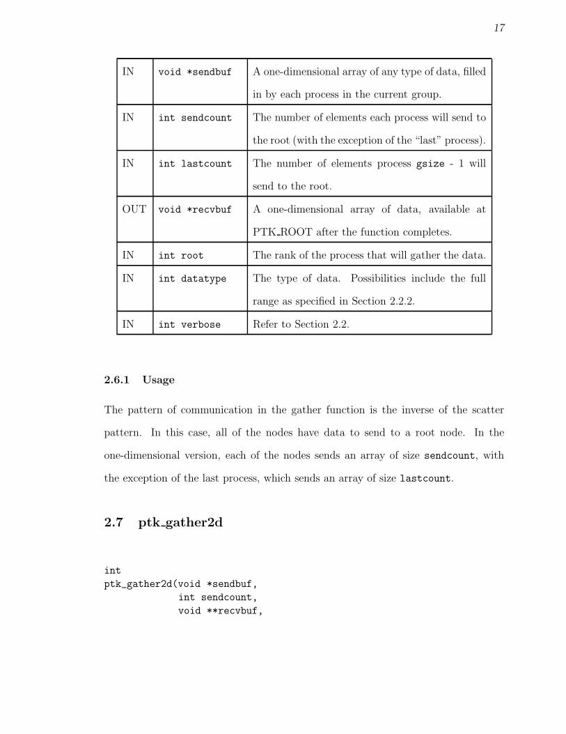
IN void *sendbuf A one-dimensional array of any type of data, filled
in by each process in the current group.
IN int sendcount The number of elements each process will send to
the root (with the exception of the “last” process).
IN int lastcount The number of elements process gsize - 1 will
send to the root.
OUT void *recvbuf A one-dimensional array of data, available at
PTK ROOT after the function completes.
IN int root The rank of the process that will gather the data.
IN int datatype The type of data. Possibilities include the full
range as specified in Section 2.2.2.
IN int verbose Refer to Section 2.2.
2.6.1 Usage
The pattern of communication in the gather function is the inverse of the scatter
pattern. In this case, all of the nodes have data to send to a root node. In the
one-dimensional version, each of the nodes sends an array of size sendcount, with
the exception of the last process, which sends an array of size lastcount.
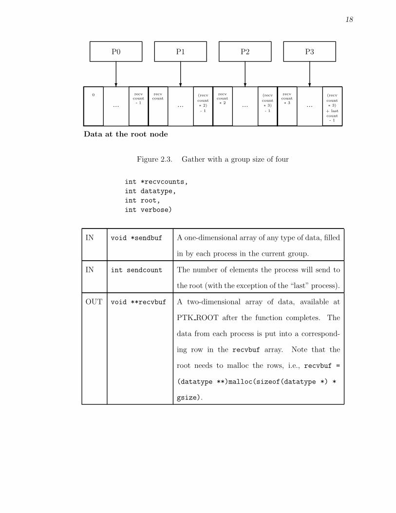
2.7 ptk gather2d
int
ptk_gather2d(void *sendbuf,
int sendcount,
void **recvbuf,
18
Data at the root node
... ... ... ...
? ? ? ?
P0 P1 P2 P3
0 recvcount- 1
recvcount
(recv
count∗ 2)
- 1
recvcount∗ 2
(recv
count∗ 3)
- 1
recvcount∗ 3
(recv
count∗ 3)
+ last
count- 1
Figure 2.3. Gather with a group size of four
int *recvcounts,
int datatype,
int root,
int verbose)
IN void *sendbuf A one-dimensional array of any type of data, filled
in by each process in the current group.
IN int sendcount The number of elements the process will send to
the root (with the exception of the “last” process).
OUT void **recvbuf A two-dimensional array of data, available at
PTK ROOT after the function completes. The
data from each process is put into a correspond-
ing row in the recvbuf array. Note that the
root needs to malloc the rows, i.e., recvbuf =
(datatype **)malloc(sizeof(datatype *) *
gsize).
19
OUT int
*recvcounts
An integer array of length group size. The
calling function at PTK ROOT must malloc, i.e.,
recvcounts = (int *)malloc(sizeof(int) *
gsize). The root will fill in the array with the
number of elements recv’d from each member,
where a row index corresponds to a process.
IN int root The rank of the process that will gather the data.
IN int datatype The type of data. Possibilities include the full
range as specified in Section 2.2.2.
IN int verbose Refer to Section 2.2.
2.7.1 Usage
In this version of gather, each process sends a varying amount of data to the root
node. The communication pattern is the same as that described for a 1-dimensional
gather. The array to be sent is a one-dimensional array. That array is then put into
a two-dimensional array at the root node, with the row position corresponding to the
position of the process in the group. The number of rows in the array must be equal
to the number of processes in the group. The size of the array to be sent is specified
in the sendcount parameter.
A two dimensional array is also passed in at PTK ROOT. The pointers to each
row in this array must be malloc’d at the root by the calling function. The toolkit
then allocates memory for each row as it is received. There is no way for the calling
function to allocate memory for each row, because it does not necessarily know how
big each row will be. The toolkit then fills in the recvcounts array, which specifies

20
how many elements are created in each row of the recvbuf array.
The calling function must specify the datatype of the send and receive buffers.
This information is used to select the appropriate pvm pack and unpack function,
and to determine the size of the data.
2.8 ptk alltoall1d
int
ptk_alltoall1d(void *sendbuf,
int sendcount,
int lastcount,
void *recvbuf,
int datatype,
int verbose)
IN void *sendbuf A one-dimensional array of any type of data, filled
in by each process in the current group.
IN int count The number of elements each process will send to
every other process.
OUT void *recvbuf A one-dimensional array of data, available at each
node after the function completes. This array con-
tains each set of data collected from every process.
The data is ordered according to process, i.e., the
set of data in the third “chunk” corresponds to
the data collected from process 3.
IN int datatype The type of data. Possibilities include the full
range as specified in Section 2.2.2.
IN int verbose Refer to Section 2.2.

21
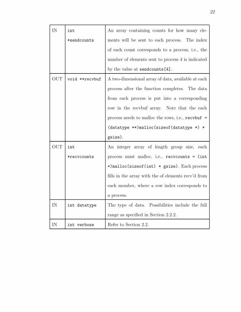
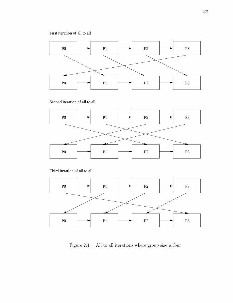
2.8.1 Usage
In an all to all communication pattern, each group member sends and receives a
message from each other group member. In this version of all to all, the assumption is
that each process sends and receives the same quantity of data. The group members
must allocate memory for their send and receive buffers. The calling function is
responsible for doing this memory allocation. The send buffer is a 1-dimensional
array of homogenous data.
In the main loop of the code, each process walks through a for loop, with the
number of iterations equal to the group size. At each iteration, each process sends
to the process i processes away from it, to the right, and receives from the process i
processes away from it, to the left. The send buffer is divided into sections, with the
number of sections being N , where N is equal to the group size, and the size being
count ∗ N . Figure 2.4 shows the communication pattern at each iteration.
2.9 ptk alltoall2d
int
ptk_alltoall2d(void **sendbuf,
int *sendcounts,
void **recvbuf,
int *recvcounts,
int datatype,
int verbose)
IN void **sendbuf A two-dimensional array of any type of data, filled
in by each process in the current group.
22
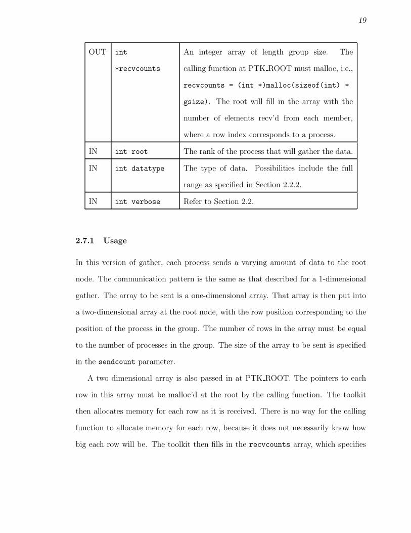
IN int
*sendcounts
An array containing counts for how many ele-
ments will be sent to each process. The index
of each count corresponds to a process, i.e., the
number of elements sent to process 4 is indicated
by the value at sendcounts[4].
OUT void **recvbuf A two-dimensional array of data, available at each
process after the function completes. The data
from each process is put into a corresponding
row in the recvbuf array. Note that the each
process needs to malloc the rows, i.e., recvbuf =
(datatype **)malloc(sizeof(datatype *) *
gsize).
OUT int
*recvcounts
An integer array of length group size, each
process must malloc, i.e., recvcounts = (int
*)malloc(sizeof(int) * gsize). Each process
fills in the array with the of elements recv’d from
each member, where a row index corresponds to
a process.
IN int datatype The type of data. Possibilities include the full
range as specified in Section 2.2.2.
IN int verbose Refer to Section 2.2.
23
P0 P1 P2 P3
P0 P1 P2 P3
First iteration of all to all
P0 P1 P2 P3
P0 P1 P2 P3
Third iteration of all to all
P0 P1 P2 P3
P0 P1 P2 P3
Second iteration of all to all
Figure 2.4. All to all iterations where group size is four
24
2.9.1 Usage
In this version of all to all, each process sends a varying amount of data to each
other process. The communication pattern is the same as that described for a 1-
dimensional all to all. The array that is passed in to be sent is a two-dimensional
array. The number of rows in the array must be equal to the number of processes in
the group. Another array is passed in, called sendcounts. This array specifies how
many elements there are in each row of the sendbuf.
Another two-dimensional array is also passed in, for the process to receive data.
The pointers to each row in this array must be malloc’d by the calling function. The
toolkit then allocates memory for each row as it is received. There is no way for
the calling function to allocate memory for each row, because it does not necessarily
know how big each row will be. The toolkit then fills in the recvcounts array, which
specifies how many elements are created in each row of the recvbuf array.
The calling function must specify the datatype of the send and receive buffers.
This information is used to select the appropriate pvm pack and unpack function,
and to determine the size of the data.
2.10 ptk mcast
int ptk_mcast(void *data,
int count,
int datatype,
int sender)
25
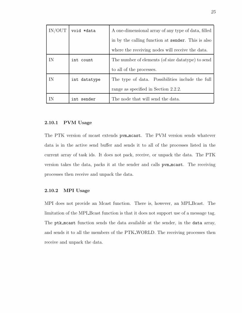
IN/OUT void *data A one-dimensional array of any type of data, filled
in by the calling function at sender. This is also
where the receiving nodes will receive the data.
IN int count The number of elements (of size datatype) to send
to all of the processes.
IN int datatype The type of data. Possibilities include the full
range as specified in Section 2.2.2.
IN int sender The node that will send the data.
2.10.1 PVM Usage
The PTK version of mcast extends pvm mcast. The PVM version sends whatever
data is in the active send buffer and sends it to all of the processes listed in the
current array of task ids. It does not pack, receive, or unpack the data. The PTK
version takes the data, packs it at the sender and calls pvm mcast. The receiving
processes then receive and unpack the data.
2.10.2 MPI Usage
MPI does not provide an Mcast function. There is, however, an MPI Bcast. The
limitation of the MPI Bcast function is that it does not support use of a message tag.
The ptk mcast function sends the data available at the sender, in the data array,
and sends it to all the members of the PTK WORLD. The receiving processes then
receive and unpack the data.
26
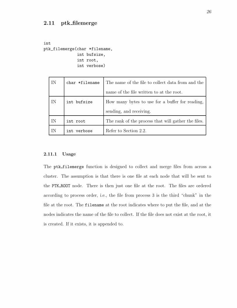
2.11 ptk filemerge
int
ptk_filemerge(char *filename,
int bufsize,
int root,
int verbose)
IN char *filename The name of the file to collect data from and the
name of the file written to at the root.
IN int bufsize How many bytes to use for a buffer for reading,
sending, and receiving.
IN int root The rank of the process that will gather the files.
IN int verbose Refer to Section 2.2.
2.11.1 Usage
The ptk filemerge function is designed to collect and merge files from across a
cluster. The assumption is that there is one file at each node that will be sent to
the PTK ROOT node. There is then just one file at the root. The files are ordered
according to process order, i.e., the file from process 3 is the third “chunk” in the
file at the root. The filename at the root indicates where to put the file, and at the
nodes indicates the name of the file to collect. If the file does not exist at the root, it
is created. If it exists, it is appended to.

27
2.12 ptk central workpool
int
ptk_central_workpool(int (*processTask)(void *task,
void **ptkResult,
int *returnSize),
int (*processResults)(void *results,
void **ptkNewTasks,
int *numNewTasks),
void *startingObjects,
int tasksize,
void (*freeObj),
int arraylen,
int granularity,
int root,
int verbose)
IN int (*processTask)() Pointer to a function that processes tasks.
This function is called by the workpool at
the worker nodes. See below for more de-
tail on what this function must support.
IN int
(*processResults)()
Pointer to a function that processes results.
This function is called by the coordinator
at the root nodes. See below for more de-
tail on what this function must support.
IN void
*startingObjects
An array of objects created by the calling
function at the root node.
IN int tasksize The size of the objects, in bytes. These are
the tasks that are processed by the pro-
cessTask function.
IN int (*freeObj()) Pointer to a function that frees and object.
28
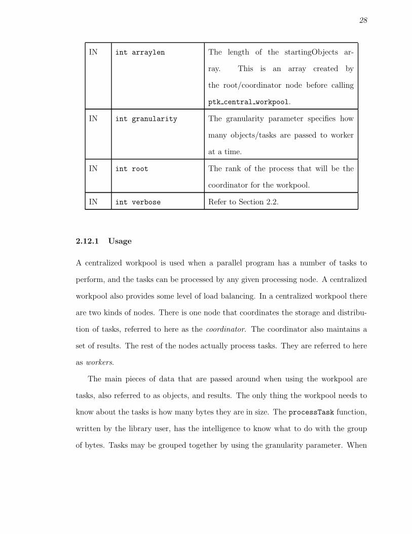
IN int arraylen The length of the startingObjects ar-
ray. This is an array created by
the root/coordinator node before calling
ptk central workpool.
IN int granularity The granularity parameter specifies how
many objects/tasks are passed to worker
at a time.
IN int root The rank of the process that will be the
coordinator for the workpool.
IN int verbose Refer to Section 2.2.
2.12.1 Usage
A centralized workpool is used when a parallel program has a number of tasks to
perform, and the tasks can be processed by any given processing node. A centralized
workpool also provides some level of load balancing. In a centralized workpool there
are two kinds of nodes. There is one node that coordinates the storage and distribu-
tion of tasks, referred to here as the coordinator. The coordinator also maintains a
set of results. The rest of the nodes actually process tasks. They are referred to here
as workers.
The main pieces of data that are passed around when using the workpool are
tasks, also referred to as objects, and results. The only thing the workpool needs to
know about the tasks is how many bytes they are in size. The processTask function,
written by the library user, has the intelligence to know what to do with the group
of bytes. Tasks may be grouped together by using the granularity parameter. When
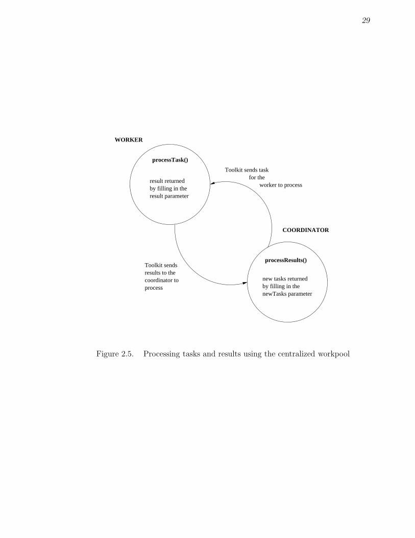
29
WORKER
COORDINATOR
result returnedby filling in theresult parameter
new tasks returnedby filling in thenewTasks parameter
Toolkit sendsresults to thecoordinator toprocess
processTask()
processResults()
for the worker to process
Toolkit sends task
Figure 2.5. Processing tasks and results using the centralized workpool
30
using the granularity parameter, tasks are sent together in “chunks.” This cuts down
on the number of messages, by passing a “chunk” of tasks together, in one message,
from the coordinator to the worker. When using the granularity parameter, the
processTask function still only needs to be able to handle one task. The task is
processed one at a time by the workpool, and results and/or new tasks dealt with
accordingly.
Note that in the following discussion of the result and task processing functions,
it of course does not matter how the user refers to each of the function’s parameters.
The user may want to use the convention presented here to help maintain clarity
about what is going on in the code.
The processTask() function
int processTask(task, ptkResult, returnSize)
void *task;
void **ptkResult;
int *returnSize;
This function must be able to process the task. If the function does not produce
any results, it may set ptkResult to null and returnSize to 0. If ptkResult is
null, but returnSize is greater than 0, nothing will be done with ptkResult by the
toolkit.
These are the same tasks that are packed by the processResults() function
into the ptkNewTasks parameter. The structure of these tasks can be anything the
calling function wants it to be. Although the user function, processResults(), may
pack many tasks into the ptkNewTasks array, only one at a time will be sent to
processTask.
31
The parameter ptkResult points to a result. This is sent to the coordinator by
the workpool. Again, the workpool does not need to know anything about what
ptkResult contains. The processResult function will get this exact set of bytes
passed in as its result parameter. The processResult function then processes the
data appropriately.
The processResult() function
int processResult(results, ptkNewTasks, numNewTasks)
void *results;
void **ptkNewTasks;
int *numNewTasks;
This function must be able to handle the results array. If it does not produce any
new tasks, it may set ptkNewTasks to null and numNewTasks to 0. If ptkNewTasks is
null, but numNewTasks is greater than 0, nothing will be done.
The parameter results is created by the processTask function and sent to the
coordinator through the workpool. It corresponds to the ptkResult parameter in the
processTask function.
The parameter ptkNewTasks points to an array of new tasks. The size should be
numNewTasks * objsize (as passed to the ptk central workpool). These tasks are
then stored by the coordinator and handed out as requested by the workers.
2.12.2 Implementation Discussion
The Coordinator
The coordinator’s reponsibility is to maintain a pool of tasks, distribute them to the
workers, process results, and terminate the function when all the tasks have been
32
completed. Tasks are stored in a circular array. The coordinator is given an initial
set of tasks to begin with, called the startingObjects. It begins by creating the
array and inserting the startingObjects into this array.
The coordinator then enters a loop, waiting for messages from the workers. The
received message may be a request for a task, or a result. If the request is for a
task, and the task array is not empty, the coordinator sends the worker a task. The
coordinator does not need to know anything about the task, other than how big it is.
If the request is a result, the coordinator calls the processResults function.
The pseudocode is as follows for the coordinator:
if (myginst == root) {
/* load array */
A = createArray;
for (i=0; i < number of startingObjects; i++) {
add task to A;
}
/* manage work */
while (finished < (gsize - 1)) {
/* receive any message from any node */
/* figure out who sent the message and what kind it is */
/* if I got the result tag, process results */
if (type of tag == RESULTTAG) {
whatToDo = processResults;
if (whatToDo == ADD_TASKS) {
for (i=0; i < number of new tasks returned; i++) {
add task to A;
}
}
else if (whatToDo == ERROR) {
deal with error;
}

33
}
else if ((type == REQUESTTAG) && !isEmpty(A)) {
pack and send tasks;
}
/* (type == REQUESTTAG) && (isEmpty(A) */
else {
finished++;
}
} /* end while-loop */
multicast the DONETAG;
/* Collect information about number of messages sent */
for (i = 0; i < gsize - 1; i++) {
receive information from all nodes about # of messages sent;
}
}
The Workers
The workers also enter a loop. They send a request for a task to the coordinator
and then receive the task. The processTask function is called. The processTask
function returns a result and sends it to the coordinator. The loop is terminated
when the worker receives a “done” signal from the coordinator.
The pseudocode for the workers is as follows:
/* else I am a worker */
else {
while (type != DONETAG) {
send request;
receive message;
if (type of message == TASKTAG) {
34
for (i=0; i < number of tasks sent; i++) {
/* compute */
whatToDo = processTask(...);
if ((whatToDo == ADD_RESULT) && (sizeReturned > 0)) {
send result to root;
}
}
}
/* if DONETAG, we are out of here */
else if (type == DONETAG) {
terminate loop;
}
} /* end while */
send root info about how many messages I sent;
}
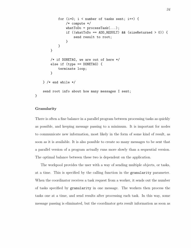
Granularity
There is often a fine balance in a parallel program between processing tasks as quickly
as possible, and keeping message passing to a minimum. It is important for nodes
to communicate new information, most likely in the form of some kind of result, as
soon as it is available. It is also possible to create so many messages to be sent that
a parallel version of a program actually runs more slowly than a sequential version.
The optimal balance between these two is dependent on the application.
The workpool provides the user with a way of sending multiple objects, or tasks,
at a time. This is specified by the calling function in the granularity parameter.
When the coordinator receives a task request from a worker, it sends out the number
of tasks specified by granularity in one message. The workers then process the
tasks one at a time, and send results after processing each task. In this way, some
message passing is eliminated, but the coordinator gets result information as soon as

35
it is available.
COORDINATORgroup "granularity" number of tasks together to send
result sent immediately after each task is processed
WORKER
for i = 0 to granularity
processTask() send result
Figure 2.6. Using granularity in the centralized workpool.
The Queue
The centralized workpool stores the tasks in a first-in, first-out queue. This is not
always ideal. There may be tasks that, if performed early in the computation, may
yield more significant results. Creating a mechanism for the user of the workpool
to indicate some priority level would mean adding a parameter to the processTask
function. This would add to the complexity of adding tasks to the queue, slowing
this process down. Solving this problem is left for future investigation.
2.13 ptk distributed workpool
int
ptk_distributed_workpool(int (*processTask)(void *dataToProcess,
int tasksToProcess,
void **ptkNewTasks,
36
int *numTasks,
void **ptkResults,
int *numResults),
int (*processResults)(void *result),
void *startingObjects,
int tasksize,
int arraylen,
int resultsize,
int granularity,
int root,
int verbose)
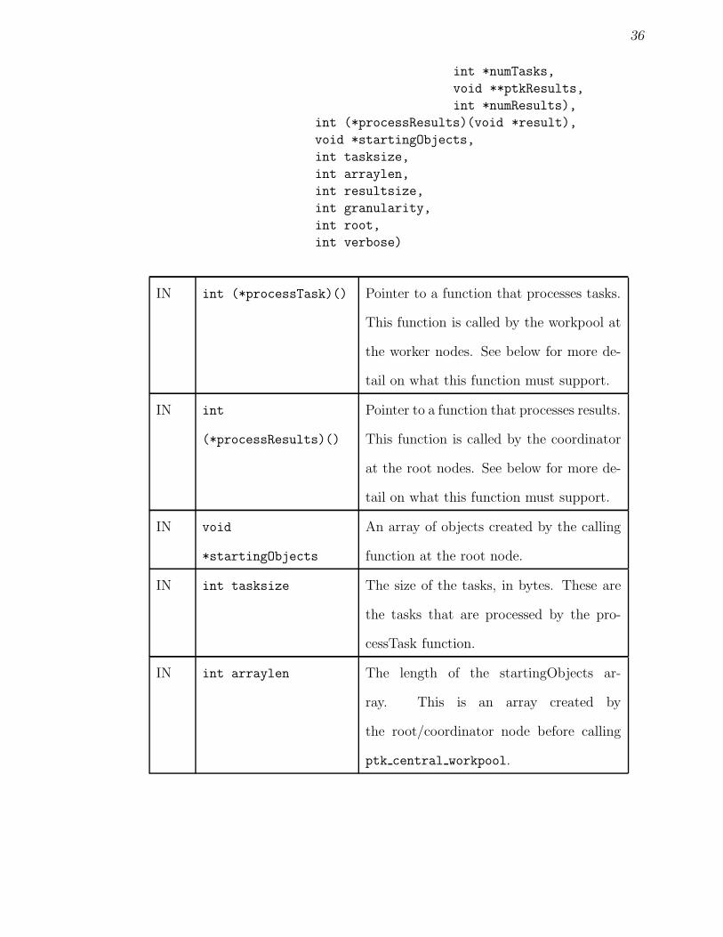
IN int (*processTask)() Pointer to a function that processes tasks.
This function is called by the workpool at
the worker nodes. See below for more de-
tail on what this function must support.
IN int
(*processResults)()
Pointer to a function that processes results.
This function is called by the coordinator
at the root nodes. See below for more de-
tail on what this function must support.
IN void
*startingObjects
An array of objects created by the calling
function at the root node.
IN int tasksize The size of the tasks, in bytes. These are
the tasks that are processed by the pro-
cessTask function.
IN int arraylen The length of the startingObjects ar-
ray. This is an array created by
the root/coordinator node before calling
ptk central workpool.

37
IN int resultsize The size of the results, in bytes. These
are the results that are processed by the
processResult function.
IN int granularity The granularity parameter specifies how
many objects/tasks are passed to worker
at a time.
IN int root The rank of the process that will be coor-
dinate termination for the workpool.
IN int verbose Refer to Section 2.2.
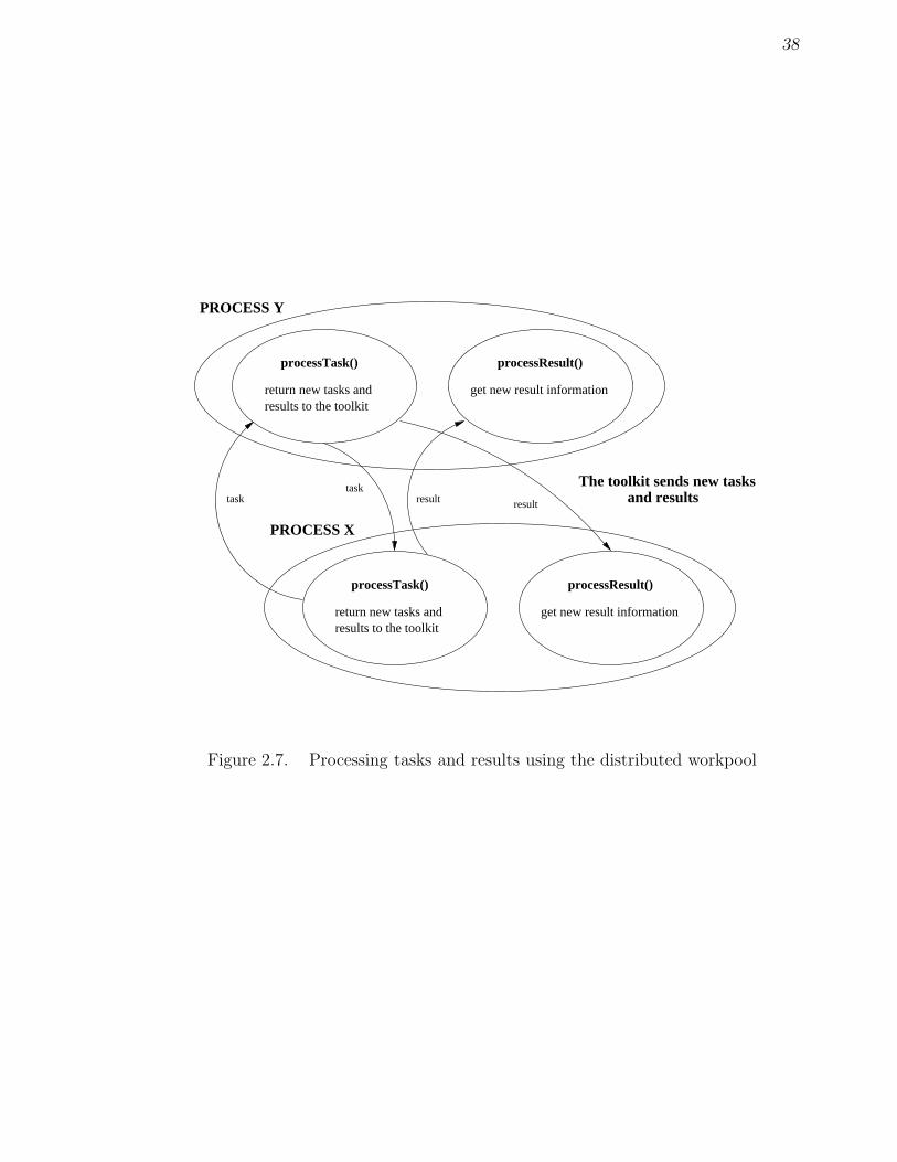
2.13.1 Usage
A distributed work pool is used when tasks can be divided up between processes. It
is also helpful where one can’t use a centralized workpool because the data needed to
process tasks cannot be stored on one processing node because of memory limitations.
The tasks must be divided in a way that each worker knows where to send new tasks
that might be created when it is processing a task. In the distributed version of
the workpool, all of the nodes are workers. There is one root node that coordinates
termination.
As in the centralized workpool, the main pieces of data that are passed between
nodes are tasks and results. The only thing the workpool needs to know about the
tasks is how many bytes they are in size. The processTask function, written by the
library user, has the intelligence to know what to do with the group of bytes. The
distributed version of the workpool also supports the granularity parameter.
Note that in the following discussion of the result and task processing functions,
38
processTask()
return new tasks andresults to the toolkit
processResult()
get new result information
PROCESS Y
processTask()
return new tasks andresults to the toolkit
processResult()
get new result information
PROCESS X
The toolkit sends new tasksand resultsresult resulttask
task
Figure 2.7. Processing tasks and results using the distributed workpool
39
it of course does not matter how the user refers to each of the function’s parameters.
The user may want to use the convention presented here to help maintain clarity
about what is going on in the code.
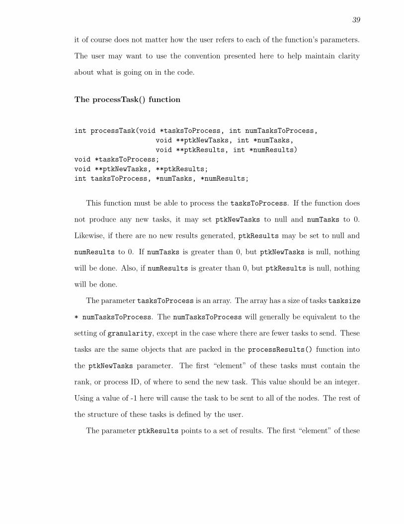
The processTask() function
int processTask(void *tasksToProcess, int numTasksToProcess,
void **ptkNewTasks, int *numTasks,
void **ptkResults, int *numResults)
void *tasksToProcess;
void **ptkNewTasks, **ptkResults;
int tasksToProcess, *numTasks, *numResults;
This function must be able to process the tasksToProcess. If the function does
not produce any new tasks, it may set ptkNewTasks to null and numTasks to 0.
Likewise, if there are no new results generated, ptkResults may be set to null and
numResults to 0. If numTasks is greater than 0, but ptkNewTasks is null, nothing
will be done. Also, if numResults is greater than 0, but ptkResults is null, nothing
will be done.
The parameter tasksToProcess is an array. The array has a size of tasks tasksize
* numTasksToProcess. The numTasksToProcess will generally be equivalent to the
setting of granularity, except in the case where there are fewer tasks to send. These
tasks are the same objects that are packed in the processResults() function into
the ptkNewTasks parameter. The first “element” of these tasks must contain the
rank, or process ID, of where to send the new task. This value should be an integer.
Using a value of -1 here will cause the task to be sent to all of the nodes. The rest of
the structure of these tasks is defined by the user.
The parameter ptkResults points to a set of results. The first “element” of these
40
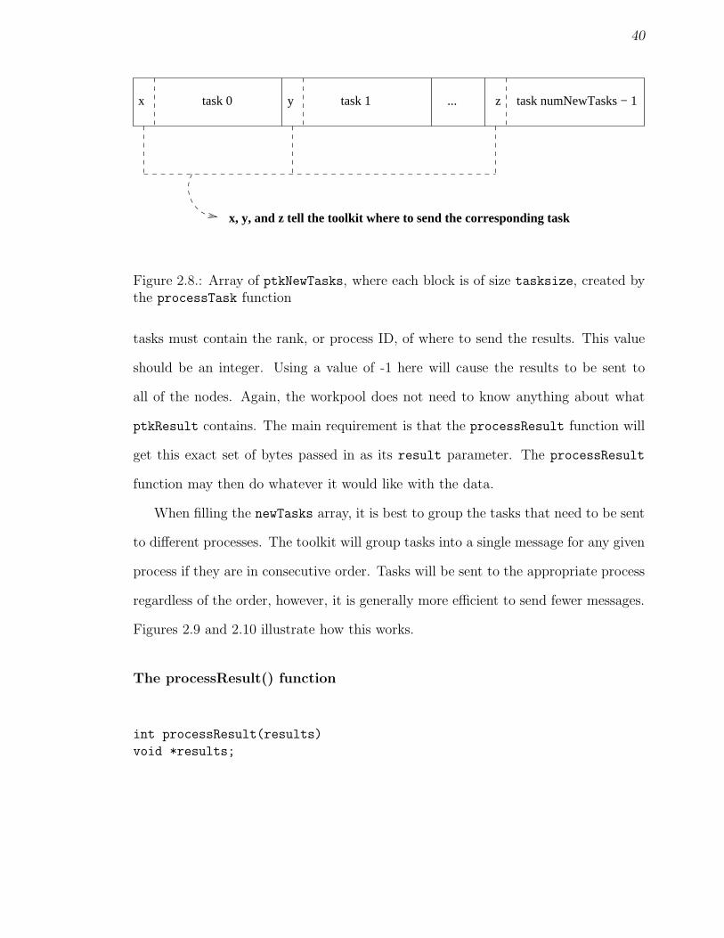
x task numNewTasks − 1...task 0 task 1y z
x, y, and z tell the toolkit where to send the corresponding task
Figure 2.8.: Array of ptkNewTasks, where each block is of size tasksize, created bythe processTask function
tasks must contain the rank, or process ID, of where to send the results. This value
should be an integer. Using a value of -1 here will cause the results to be sent to
all of the nodes. Again, the workpool does not need to know anything about what
ptkResult contains. The main requirement is that the processResult function will
get this exact set of bytes passed in as its result parameter. The processResult
function may then do whatever it would like with the data.
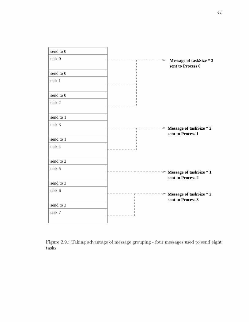
When filling the newTasks array, it is best to group the tasks that need to be sent
to different processes. The toolkit will group tasks into a single message for any given
process if they are in consecutive order. Tasks will be sent to the appropriate process
regardless of the order, however, it is generally more efficient to send fewer messages.
Figures 2.9 and 2.10 illustrate how this works.
The processResult() function
int processResult(results)
void *results;
41
send to 0
task 0
send to 0
task 2
send to 1
task 3
send to 1
task 4
send to 2
task 5
send to 3
task 6
send to 0
task 1
Message of taskSize * 2sent to Process 1
Message of taskSize * 1sent to Process 2
Message of taskSize * 2sent to Process 3
Message of taskSize * 3sent to Process 0
send to 3
task 7
Figure 2.9.: Taking advantage of message grouping - four messages used to send eighttasks.

42
send to 0
task 0
send to 2
task 2
send to 3
task 3
send to 0
task 4
send to 1
task 5
send to 2
task 6
send to 1
task 1
Message sent to Process 0
Message sent to Process 2
Message sent to Process 1
Message sent to Process 0
Message sent to Process 1
Message sent to Process 2
Message sent to Process 3
Message sent to Process 3
task 7
send to 3
Figure 2.10.: Not taking advantage of message grouping - eight messages used to sendeight tasks.
43
This function must be able to handle the results array. Generally speaking,
in a distributed workpool, all of the nodes maintain a current best set of results.
As new results are generated, they are sent out to the other nodes. The results
array is created by the processTask function and sent to the other nodes through
the workpool. It corresponds to the ptkResults parameter in the processTask
function.
2.13.2 Implementation Discussion
The communication pattern in the distributed workpool is completely asynchronous,
and the size of the messages passed varies with every send and receive. Each node
in the workpool cycles through a loop. It performs a blocking receive, waiting for a
task to arrive from another node. It then processes the task and sends out any new
tasks that result.
The pseudocode for the distributed workpool is as follows:
while (type != DONETAG) {
/* receive any message type from any node */
/* Figure out what I got, where it came from, and how big it is */
if (type == RESULTTAG) {
/* call the user function that processes the results */
}
else if (type == TASKTAG) {
nothingNew = TRUE;
/* check the granularity value, and do some math to figure out
* how many tasks to group together
*/

44
while there are tasks left to process {
/* compute */
error = (int)(*processTask)(...);
if (number of results > 0) {
send results to other nodes;
if (number of new tasks > 0) {
nothingNew = FALSE;
send new tasks to other nodes;
}
/* If nothing generated, and I’m the root, I’m done,
* change color to white */
if ((nothingNew == TRUE) &&
(me == root) && (sentTokens == 0)) {
token = WHITE;
send the token;
}
}
else if (type == TOKENTAG) {
copy the token out of the receive buffer;
if (me == root) {
if (token == WHITE) {
/* If the root gets a white token, we are done */
multicast the DONETAG;
}
else {
/* The root always sends a white token */
token = WHITE;
send the token;
}
}
else {
if (color == BLACK) {
token = BLACK;
}
send the token;
color = WHITE;
}
}
/* if DONETAG, we are out of here */
else if (type == DONETAG) {
45
leave the loop;
}
else if (type == DIETAG) {
goto done;
}
} /* end while */
Task Objects
The tasks that are passed between worker processes contain an integer followed by
any number of bytes. The integer at the beginning of the task object is required by
the workpool. This integer indicates to the workpool the id of the process that the
task should be sent to. The calling function indicates the size of the object in the
tasksize parameter. This tasksize should include the size of the integer that is at
the beginning of the task object.
Grouping Messages
When a process sends new tasks or results to the other processes, it groups the
messages for each process together. For example, if P1 has five new tasks for P2, it
will send one message containing all five new tasks if these five tasks are sequential in
the ptkNewTasks array. This significantly cuts down on message passing. P2 will then
process the first task, broadcast results, process the second task, broadcast results,
etc.
Load Balancing
The distributed workpool does not load balance. It simply sends new tasks where it is
told to send them. The workpool could monitor the load at each node by tracking idle
time. If a process were idle for some designated time, it could send out a message that

46
it needed work. The user of the toolkit could then handle the situation appropriately.
How to load balance when tasks are distributed between nodes is very dependent on
the application. At most the toolkit could signal that processes are idle. Adding load
balancing to the distributed workpool was deemed beyond the scope of this project
and is left for future experimentation.
Termination Detection
Pj PiP0 Pn−1
Task
white token white tokenPi turns white token black
Figure 2.11. Dual-pass token ring termination algorithm
The distributed workpool uses a dual-pass token ring algorithm originally devel-
oped by Dijkstra, Feijen, and van Gasteren [2], as illustrated in Figure 2.11. This
algorithm is used instead of a single-pass token ring because processes may be reac-
tivated after receiving and passing a token. Each process keeps track of its “color.”
The color is either white or black. The processes pass tokens to their neighbors to
the right. The algorithm is described as follows:
1. All processes initialize their color to white.
2. When P0 runs out of tasks, i.e., there are no tasks in the receive buffer, it sends

47
a white token to P1.
3. Whenever a process sends a task to a neighbor to its left, it colors itself black.
As a process terminates, it receives the token from its neighbor to its left. If the
received token is white and the process’ color is white, it passes on the white
token. If the received token is white and the process’ color is black, it turns the
token black and passes it on. It the token is black, it will be passed on as is,
regardless of the color of the process. After a process passes on the token, it
changes its color to white.
4. When P0 receives a white token, that means that all of the processes have termi-
nated and none of them have been reactivated, thus terminating the workpool.
The Big Problem, or How Unordered Messages Caused Great Headache
I wrote the first version of the toolkit in PVM, and then ported the functions to
MPI. PVM and MPI have slightly different versions of send. In PVM, to perform a
blocking receive of a message, one first calls pvm recv, and then follows it with a call
to pvm unpack to get the data into a buffer. To do the same thing in MPI, one first
calls MPI Probe which blocks until a message is received. Then MPI Recv is called to
get the data. In doing the port, I simply changed the pvm recv calls to MPI Probe
calls, and the pvm unpacks to MPI Recvs. In the process of porting the distributed
workpool to MPI I ran into a problem caused by an issue referred to earlier. As
discussed in Section 2.1, PVM guarantees message ordering, while MPI does not.
After making these changes to the distributed workpool, my MPI version wouldn’t
run with the example code. I determined that the problem was that I ran into a
situation where two processes were doing blocking sends to each other, causing a

48
deadlock. This was a symptom of the difference in the way that PVM and MPI
handle message ordering.
The question then was how to get around this. One option was to do a non-
blocking send and then a wait, which blocks until the message was received. This,
of course, produced the exact same problem. After experimenting with a number of
different options, I came up with what I believe to be a rather novel solution.
I changed the sends to non-blocking sends (MPI Isend). The only problem with
this is that you can’t touch the send buffer until it has been received. Since I needed
to free the memory I’d used for the buffer I somehow needed to keep track of it. The
non-blocking send provides, as a function parameter, a “handle” to the send buffer.
This handle is represented by the MPI Request datatype. There is an MPI function
that allows you to get status information about a certain MPI Request.
To solve my problem, I store a list of MPI Requests in a circular array after each
send. I also store a list of buffer pointers in a second array. When a process is idle,
i.e., there are no messages waiting for it, it runs through the array and calls MPI Test
to check the status of the MPI Requests. If the message has been received, it frees
the memory and removes the structure from the array. In the first incarnation of
this solution, I ran through the whole array every time. This caused the code to take
forever to run. I discovered that only the first few tests in the array were encountering
received messages. I changed it so that once a non-received message is found, the loop
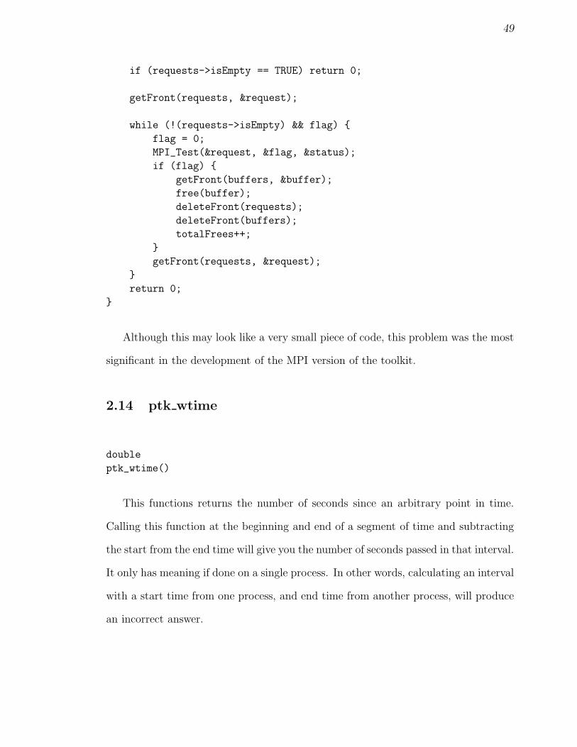
terminates. The code is as follows:
int cleanup() {
int flag = 1;
MPI_Status status;
MPI_Request request;
void *buffer = NULL;
49
if (requests->isEmpty == TRUE) return 0;
getFront(requests, &request);
while (!(requests->isEmpty) && flag) {
flag = 0;
MPI_Test(&request, &flag, &status);
if (flag) {
getFront(buffers, &buffer);
free(buffer);
deleteFront(requests);
deleteFront(buffers);
totalFrees++;
}
getFront(requests, &request);
}
return 0;
}
Although this may look like a very small piece of code, this problem was the most
significant in the development of the MPI version of the toolkit.
2.14 ptk wtime
double
ptk_wtime()
This functions returns the number of seconds since an arbitrary point in time.
Calling this function at the beginning and end of a segment of time and subtracting
the start from the end time will give you the number of seconds passed in that interval.
It only has meaning if done on a single process. In other words, calculating an interval
with a start time from one process, and end time from another process, will produce
an incorrect answer.
50
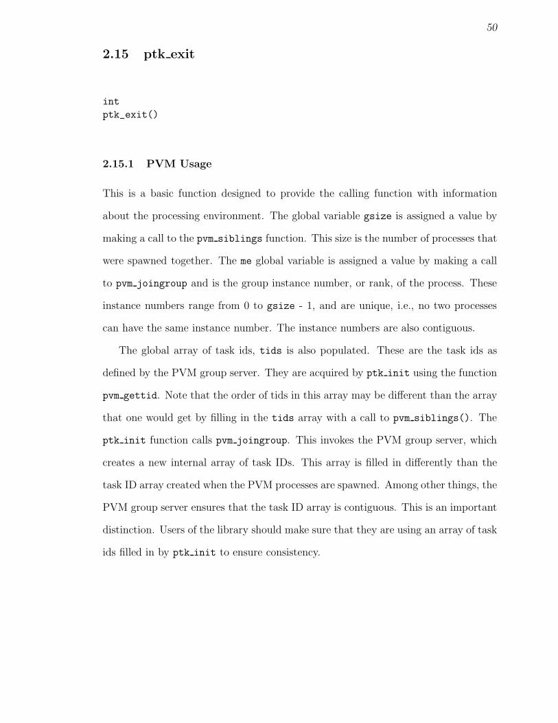
2.15 ptk exit
int
ptk_exit()
2.15.1 PVM Usage
This is a basic function designed to provide the calling function with information
about the processing environment. The global variable gsize is assigned a value by
making a call to the pvm siblings function. This size is the number of processes that
were spawned together. The me global variable is assigned a value by making a call
to pvm joingroup and is the group instance number, or rank, of the process. These
instance numbers range from 0 to gsize - 1, and are unique, i.e., no two processes
can have the same instance number. The instance numbers are also contiguous.
The global array of task ids, tids is also populated. These are the task ids as
defined by the PVM group server. They are acquired by ptk init using the function
pvm gettid. Note that the order of tids in this array may be different than the array
that one would get by filling in the tids array with a call to pvm siblings(). The
ptk init function calls pvm joingroup. This invokes the PVM group server, which
creates a new internal array of task IDs. This array is filled in differently than the
task ID array created when the PVM processes are spawned. Among other things, the
PVM group server ensures that the task ID array is contiguous. This is an important
distinction. Users of the library should make sure that they are using an array of task
ids filled in by ptk init to ensure consistency.
51
2.15.2 MPI Usage
The argc and argv parameters should be self explanatory. They are used in a call
to MPI Init to pass parameters to all the processes. The gsize global variable is
given a value by calling MPI Comm size, and will be equivalent to all the processes
in PTK WORLD. PTK WORLD is an MPI Comm. An MPI Comm is a communi-
cator. For more discussion of communicators, refer to [6]. This function creates the
PTK WORLD from the MPI COMM WORLD. The me global variable is assigned a
value with a call to MPI Comm rank, and is the rank of the process in the group.
2.16 Miscellaneous Files Used By the Toolkit
2.16.1 ptk array
This file implements a growable, circular array. It is used to maintain the queue
of tasks in the centralized workpool, and the queue of message handles and buffer
pointers in the distributed workpool. It is not necessary for the user of the library to
understand or use this code.
2.16.2 ptk pvmgs
The functions used from this file include gs get datasize(int datatype), which
returns the size of datatype. The other function in this file is gs pack unpack(int
datatype, int (**packfunc)(), int (**unpackfunc)()). It is used to find the
appropriate PVM pack and unpack functions for the specified datatype. This code
was borrowed from the PVM source code.

52
Chapter 3
USING THE TOOLKIT: SOME EXAMPLES
This chapter contains documentation for a number of different example programs.
The code is provided as part of the toolkit package. The code can be downloaded
from:
http://cs.boisestate.edu/~amit/research/ptk.
In that directory there are two subdirectories, one is pvm, the other is mpi.
3.1 Gather and Scatter
3.1.1 A Simple One-Dimensional Gather
This example may be found in $PTK HOME/examples/gather1d.c. In this very simple
example a series of N numbers is gathered from the nodes by the root. Each node
generates a sequence of numbers from process id number * sendcount to (process id
number * sendcount) + sendcount - 1, where sendcount is equivalent to N / group
size. These numbers fill the sendbuf array. It is obvious that the memory for the
sendbuf needs to be malloc’d by each node. Note that the memory for recvbuf is
also malloc’d, by the root, even though the toolkit will fill it in for us.
The program then calls ptk gather1d to gather the data. After the function
returns, the root should then have in its recvubf numbers in the range of 0 to N .
Note that since we malloc’d the memory for the send and receive buffers we free it
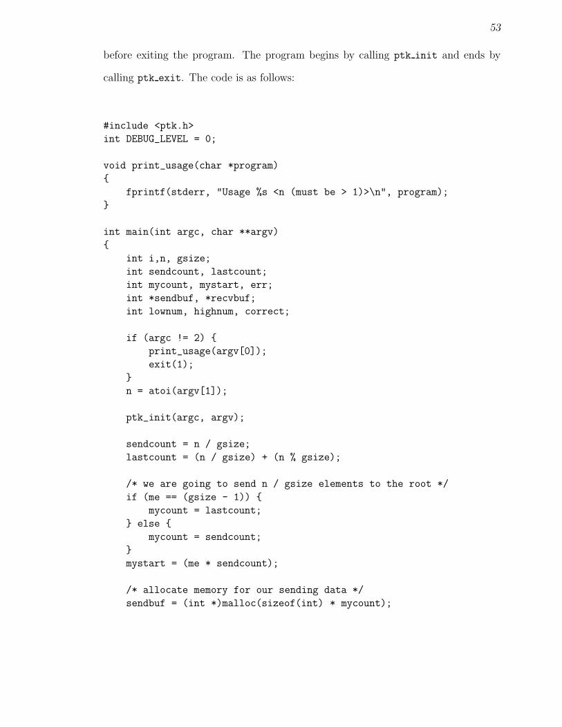
53
before exiting the program. The program begins by calling ptk init and ends by
calling ptk exit. The code is as follows:
#include <ptk.h>
int DEBUG_LEVEL = 0;
void print_usage(char *program)
{
fprintf(stderr, "Usage %s <n (must be > 1)>\n", program);
}
int main(int argc, char **argv)
{
int i,n, gsize;
int sendcount, lastcount;
int mycount, mystart, err;
int *sendbuf, *recvbuf;
int lownum, highnum, correct;
if (argc != 2) {
print_usage(argv[0]);
exit(1);
}
n = atoi(argv[1]);
ptk_init(argc, argv);
sendcount = n / gsize;
lastcount = (n / gsize) + (n % gsize);
/* we are going to send n / gsize elements to the root */
if (me == (gsize - 1)) {
mycount = lastcount;
} else {
mycount = sendcount;
}
mystart = (me * sendcount);
/* allocate memory for our sending data */
sendbuf = (int *)malloc(sizeof(int) * mycount);
54
if (me == PTK_ROOT) {
recvbuf = (int *)malloc(sizeof(int) * n);
}
/* fill up the array */
for (i = 0; i < mycount; i++) {
sendbuf[i] = i + mystart;
}
/* send the data to the root */
err = ptk_gather1d(sendbuf, sendcount, lastcount,
recvbuf, PVM_INT, 0);
if (me = PTK_ROOT) {
correct = 1;
/* make sure that I got the correct numbers */
if (err < 0) {
fprintf(stderr, "err at p%d from ptk_gather = %d",
myginst, err);
} else {
for (i = 0; i < n; i++) {
if (recvbuf[i] != i) {
fprintf(stderr, "recvbuf[%d] = %d\n",
i, recvbuf[i]);
correct = 0;
}
}
}
}
free(sendbuf);
free(recvbuf);
ptk_exit();
if (correct != 1) {
fprintf(stderr, "Error all to all at p%d when n = %d!!\n",
myginst, n);
exit(-1);
} else {
exit(0);
}
}
55
3.1.2 A One-Dimensional Scatter Example
This example may be found in $PTK HOME/examples/shortestPathsDistributed.c.
The one-dimensional scatter, ptk scatter1d is used in the distributed workpool
shortest paths examples. It is used to distribute the edge data to all of the nodes. In
this example, a one-dimensional array is filled with data, a portion of which is needed
by each node. For more information on the distributed shortest paths example see
Section 3.4.3.
3.1.3 Bucketsort Using Two-Dimensional Scatter
This example may be found in $PTK HOME/examples/bucketSortWithScatter.c.
This example shows how to use a two-dimensional scatter function. In this version of
bucket sort, a quantity of N numbers is sorted. In this example, the root node begins
by generating N random numbers. As the numbers are generated, they are added to
the appropriate row of a two-dimensional array, where the row index corresponds to
a process node that will get the data.
After the numbers are generated, ptk scatter2d is called to distribute the data.
After the scatter is called, memory is free’d at the root. A bucket sorting function is
then called to sort the received data at each of the nodes. After the sort, each node
verifies that its data is sorted. The root node also verifies that data is sorted across
rows, i.e., the largest number at Pi is less than the smallest number at Pi − 1. For
more information on the bucket sort algorithm, see Cormen, Leiserson, et al [1].
56
3.2 All to All
3.2.1 A Simple All to All
This example may be found in $PTK HOME/examples/allToall.c. This is another
simple example. In this case a one-dimensional array of data is distributed across a
group of processes. Two arrays are defined, sendbuf and recvbuf. It is obvious that
the memory for the sendbuf needs to be malloc’d by the sending node. Note that the
memory for recvbuf is also malloc’d, even though the toolkit will fill it in for us.
The sendbuf is then filled with numbers, where the data at each index in the
array is equal to the index, i.e., i[3] = 3. The program then calls ptk alltoall1d to
distribute the data. Each processing node should then have in its recvubf numbers
in the range of (process id number * sendcount) to ((process id number * sendcount)
+ sendcount - 1).
Note that since we malloc’d the memory for the send and receive buffers we free
it before exiting the program. The program begins by calling ptk init and ends by
calling ptk exit.
3.2.2 Bucketsort Using All to All
This example may be found in $PTK HOME/examples/bucketSortWithAlltoAll2d.c.
This is a more interesting example of how to use an all to all function. In this version
of bucket sort, a quantity of N numbers is sorted. Each process node begins by
generating N/groupsize random numbers, using a parallel random number generator,
prand. The prand library is available at:
http://cs.boisestate.edu/~amit/research/prand.
Each node is responsible for sorting numbers in a certain range. The range is
57
equivalent to (RANDMAX/groupsize)∗processID) to (RANDMAX/groupsize)∗
processID+1)−1. As the numbers are generated, they are added to the appropriate
row of a two-dimensional array, where the row index corresponds to a process node
that will get the data.
After the numbers are generated, ptk alltoall2d is called to distribute the data.
After the all to all is called, memory is free’d. A bucket sorting function is then called
to sort the received data. After the sort, each node verifies that its data is sorted.
The root node also verifies that data is sorted across rows, i.e., the largest number
at Pi is less than the smallest number at Pi − 1. For more information on the bucket
sort algorithm, see Cormen, Leiserson, et al [1].
3.3 Merging Files From Across a Cluster
This example may be found in $PTK HOME/examples/filemerge.c. This program
merges N files from across a cluster, where the number of processes is equal to N .
The first argument is the name of the file to collect from the non-root nodes. The
second argument is the name of the file to collect the data into at the root. The third
is the size of the buffer to use, and the fourth is the process ID of the root node.
Each node calculates the size of its file and sends that size information to the
root. The ptk filemerge function is then called. When the function returns, the
root checks the size of the newly collected file. It verifies that the size of the new file
is the same as the calculated total of all the size information received.
58
3.4 The Workpools
3.4.1 Choosing the Appropriate Workpool
It is important to understand the major differences between the centralized and dis-
tributed workpools when deciding which to use. A workpool should be used when a
problem lends itself to a divide and conquer technique. The example shown with the
toolkit is the problem of finding shortest paths in a graph, using Moore’s algorithm.
It is helpful for the reader to understand the algorithm in the following discussion. A
simple explanation of Moore’s algorithm is put forth in Wilkinson and Allen [13]:
Starting with the source vertex, the basic algorithm implemented whenvertex i is being considered is as follows: Find the distance to vertexj through vertex i and compare with the current minimum distance tovertex j. Change the minimum distance if the distance through vertex i isshorter. In mathematical notation, if di is the current minimum distancefrom the source vertex to vertex i, and wi,j is the weight of the edge fromvertex i to vertex j, we have
dj = min(dj , di + wi,j)
If a new better distance is found for any given vertex, insert that vertexinto a queue. Keep investigating vertices in the queue until the queue isempty.
The major data structures used in the algorithm are a two-dimensional array of
edges, a one-dimensional array of current best distances, and a one-dimensional array
of the paths to those current best distances. The size of the edge array is the square
of the number of vertices in the graph. The other two arrays are equivalent in length
to the number of vertices.
59
Memory Usage
One of the big issues that arises in using a workpool is memory. Generally speaking,
when using a centralized workpool, all of the nodes need to have all of the information
required to process a task. This is because all of the nodes need to be able to process
any task. In our shortest paths example, the edge array is stored in its entirety by
each node. The distance and path array is passed as part of the task when handed
out by the coordinator. So in our example, each node needs to be able to store
vertices2 + 2vertices.
Needless to say, this quickly becomes a large amount of memory. If a graph
contains 10,000 vertices, each node will have approximately 1.5GB of data, assuming
the vertices are integers that each require 4 bytes of space. If memory at the nodes
becomes a limiting factor, then it makes sense to use the distributed version of the
workpool.
In a distributed workpool, each node is responsible for a certain subset of tasks.
In our shortest paths example, each node is responsible for a number of vertices
equivalent to vertices/groupsize. This means that each node now only needs to
store a fraction of the edge data. Each node maintains it owns set of the current
best distance and path arrays. This means that each node now only needs to store
(vertices2/groupsize) + vertices ∗ 2.
Consider our previous example of a graph containing 10,000 vertices. If we use 20
processes to search the graph, each node now only needs 76MB of memory to store
the necessary information. This is a significant improvement over our earlier 1.5GB.
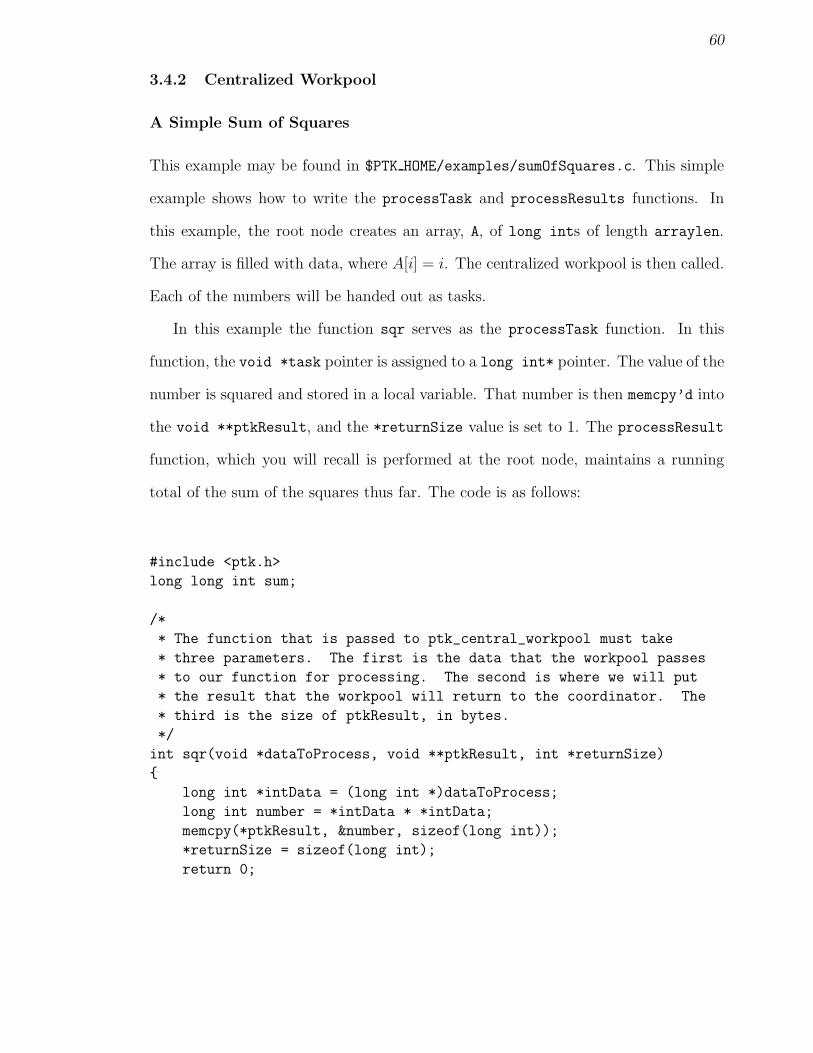
60
3.4.2 Centralized Workpool
A Simple Sum of Squares
This example may be found in $PTK HOME/examples/sumOfSquares.c. This simple
example shows how to write the processTask and processResults functions. In
this example, the root node creates an array, A, of long ints of length arraylen.
The array is filled with data, where A[i] = i. The centralized workpool is then called.
Each of the numbers will be handed out as tasks.
In this example the function sqr serves as the processTask function. In this
function, the void *task pointer is assigned to a long int* pointer. The value of the
number is squared and stored in a local variable. That number is then memcpy’d into
the void **ptkResult, and the *returnSize value is set to 1. The processResult
function, which you will recall is performed at the root node, maintains a running
total of the sum of the squares thus far. The code is as follows:
#include <ptk.h>
long long int sum;
/*
* The function that is passed to ptk_central_workpool must take
* three parameters. The first is the data that the workpool passes
* to our function for processing. The second is where we will put
* the result that the workpool will return to the coordinator. The
* third is the size of ptkResult, in bytes.
*/
int sqr(void *dataToProcess, void **ptkResult, int *returnSize)
{
long int *intData = (long int *)dataToProcess;
long int number = *intData * *intData;
memcpy(*ptkResult, &number, sizeof(long int));
*returnSize = sizeof(long int);
return 0;
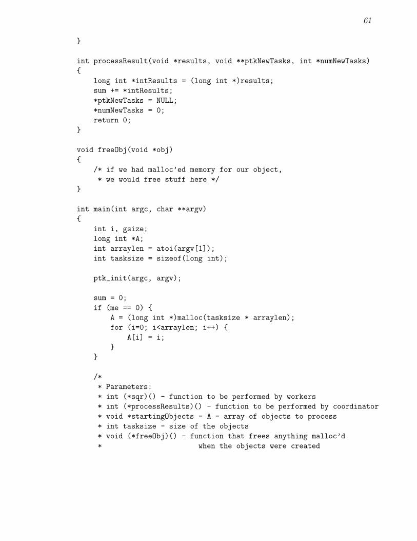
61
}
int processResult(void *results, void **ptkNewTasks, int *numNewTasks)
{
long int *intResults = (long int *)results;
sum += *intResults;
*ptkNewTasks = NULL;
*numNewTasks = 0;
return 0;
}
void freeObj(void *obj)
{
/* if we had malloc’ed memory for our object,
* we would free stuff here */
}
int main(int argc, char **argv)
{
int i, gsize;
long int *A;
int arraylen = atoi(argv[1]);
int tasksize = sizeof(long int);
ptk_init(argc, argv);
sum = 0;
if (me == 0) {
A = (long int *)malloc(tasksize * arraylen);
for (i=0; i<arraylen; i++) {
A[i] = i;
}
}
/*
* Parameters:
* int (*sqr)() - function to be performed by workers
* int (*processResults)() - function to be performed by coordinator
* void *startingObjects - A - array of objects to process
* int tasksize - size of the objects
* void (*freeObj)() - function that frees anything malloc’d
* when the objects were created
62
* int arraylen - length of the array myobjs, A in our case
* int root - 0 in this case
* int verbose - 0 for nothing, 1 for everything - will output
* information about what is happening
*/
ptk_central_workpool(sqr,
processResult,
(void *)A,
tasksize,
freeObj,
arraylen,
1, /* granularity */
0, /* root */
0); /* not verbose */
if (me == 0) {
free(A);
printf("gsize = %2d, n = %6d, sum of squares is %lld.\n",
gsize, arraylen, sum);
}
ptk_exit();
exit(0);
}
Shortest Paths Central - The Simple Version
This example may be found in $PTK HOME/examples/shortestPathsCentral.c. The
shortest paths example provides a look at a more substantial piece of code. In this
example the function processVertex serves as the processTask function. The code
for the processVertex function can be found in Section A.1.1. The task here is
composed of a vertex, represented as an int, followed by an array of ints, which
represent the current best set of distances from the source. The function begins
by memcpy’ing these values into a local vertex value, and a distances array. The
distances array is a global array, so that memory for it can be malloc’d and free’d
just once.
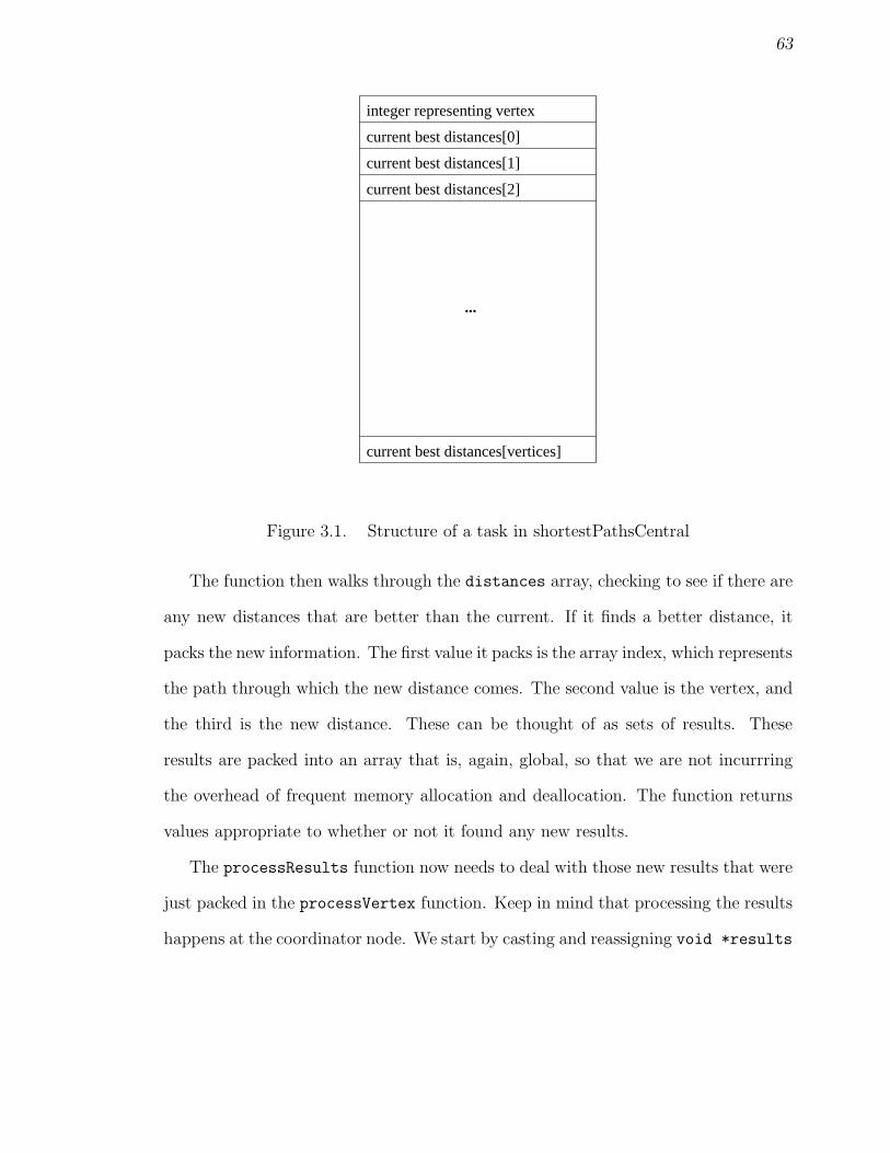
63
...
integer representing vertex
current best distances[0]
current best distances[vertices]
current best distances[1]
current best distances[2]
Figure 3.1. Structure of a task in shortestPathsCentral
The function then walks through the distances array, checking to see if there are
any new distances that are better than the current. If it finds a better distance, it
packs the new information. The first value it packs is the array index, which represents
the path through which the new distance comes. The second value is the vertex, and
the third is the new distance. These can be thought of as sets of results. These
results are packed into an array that is, again, global, so that we are not incurrring
the overhead of frequent memory allocation and deallocation. The function returns
values appropriate to whether or not it found any new results.
The processResults function now needs to deal with those new results that were
just packed in the processVertex function. Keep in mind that processing the results
happens at the coordinator node. We start by casting and reassigning void *results
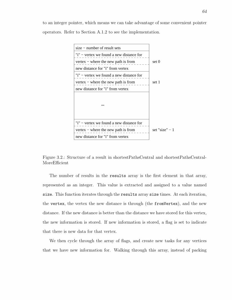
64
to an integer pointer, which means we can take advantage of some convenient pointer
operators. Refer to Section A.1.2 to see the implementation.
"i" − vertex we found a new distance for
vertex − where the new path is from
new distance for "i" from vertex
"i" − vertex we found a new distance for
vertex − where the new path is from
new distance for "i" from vertex
"i" − vertex we found a new distance for
vertex − where the new path is from
new distance for "i" from vertex
size − number of result sets
...
set 0
set 1
set "size" − 1
Figure 3.2.: Structure of a result in shortestPathsCentral and shortestPathsCentral-MoreEfficient
The number of results in the results array is the first element in that array,
represented as an integer. This value is extracted and assigned to a value named
size. This function iterates through the results array size times. At each iteration,
the vertex, the vertex the new distance is through (the fromVertex), and the new
distance. If the new distance is better than the distance we have stored for this vertex,
the new information is stored. If new information is stored, a flag is set to indicate
that there is new data for that vertex.
We then cycle through the array of flags, and create new tasks for any vertices
that we have new information for. Walking through this array, instead of packing
65
the new task immediately after discovering it, adds some small amount of overhead.
The advantage of doing it this way means that we are packing the best distances we
have for all of the results processed. In the long run this means fewer new tasks are
ultimately created.
Shortest Paths Central - A More Efficient Version
Refer to $PTK HOME/examples/shortestPathsCentralMoreEfficient.c to see the
full example. The above example is useful in understanding the workpool, but the
tasks are not computationally intensive, or in other words are very fine-grained. This
results in processes spending more time passing messages than performing actual
computations. The following example tries to solve this problem by grouping vertices
to examine into larger tasks, so that with each task we are performing more compu-
tation. In this example the function processVertex (see Section A.2.1) serves as the
processTask function. The task is structured as seen in Figure 3.3.
The task is composed of an array of integers, which represents the current best
set of distances, an integer equivalent to the number of vertices to check, followed
by this number of vertices. The function begins by memcpy’ing the distances into the
global distances array. It then fills in the verticesToCheck value with the integer
following the distances array. The distances array is again a global array.
The function then iterates from 0 to verticesToCheck. It copies the vertex to
investigate into the vertex value. It then walks through the distances array to see if
the new distance improves any other paths, as was done in the basic shortest paths
centralized version.
The processResult function is very similar to the basic shortest paths central
version. The code for processResult may be found in Section A.2.2. The exception
66
is in how it repacks the task. Since the tasks are grouped, we need to do that here.
The value verticesPerTask is passed in at the command line of the main program.
It specifies how many vertices are to be packed into any given task. The only tricky
part of packing the tasks is accounting for any number of vertices left if the number
of vertices we need to pack up is not evenly divided by verticesPerTask. These
calculations are made, and the tasks are packed.
3.4.3 Distributed Workpool
Shortest Paths Distributed - The Simple Version
This example may be found in $PTK HOME/examples/shortestPathsDistributed.c.
This version of shortest paths is distributed. Each of the processes has a certain
“slice” of vertices that it is responsible for processing. This slice is equivalent to
vertices/number of processes in group. The processVertex function(Section A.3)
is similar to that in the centralized shortest paths in process, however the task is
structured very differently. Because each process keeps its own current set of best
results, the entire distance array does not need to be sent as part of the task. The
structure of the task is shown in Figure 3.4.
This function begins by “unpacking” the vertex, path, and distance information
from the task. It iterates through its current best distances array to see if the new
vertex information creates any new tasks. As it finds new tasks it packs them up.
The newTasks array is global, again to avoid frequent allocation and deallocation of
memory. Each new task contains information about the process to send the new task
to, the vertex, the path, and the new distance, as pictured in Figure 3.5.
After the new tasks are packed up the new results need to be broadcast to all of
the other nodes. The first element of ptkResults is where to send the information.
67
We use a -1 here to signal the toolkit to broadcast the data to all of the nodes. The
next set of numbers is the distance array, followed by the paths array. In this
example, numResults is always 1.
Processing the results, which happens at each node, is very simple. The func-
tion simply iterates through the new distances received, compares them to its own
current best data, and replaces any values that are better than the current. The
processResult function code may be seen in Section A.3.2.
Shortest Paths Distributed - A More Efficient Version
Refer $PTK HOME/examples/shortestPathsDistributedMoreEfficient.c for the full
implementation of this example. The shortest paths distributed more efficient ver-
sion takes advantage of the workpool’s granularity functionality. In this version, we
assume that tasksToProcess will be greater than one. We do what was done in the
more efficient version of the centralized shortest paths example. Instead of examining
just one vertex, we iterate through a loop and examine vertices, setting a flag when
we find a new and better distance. We then iterate through our array of flags, and
pack any new information into ptkNewTasks. The structure of ptkNewTasks is the
same as in the simple version. The code for the processVertex function may be
found in Section A.4.1.
The processing of the result in the shortest paths distributed more efficient exam-
ple is identical to the simple version.
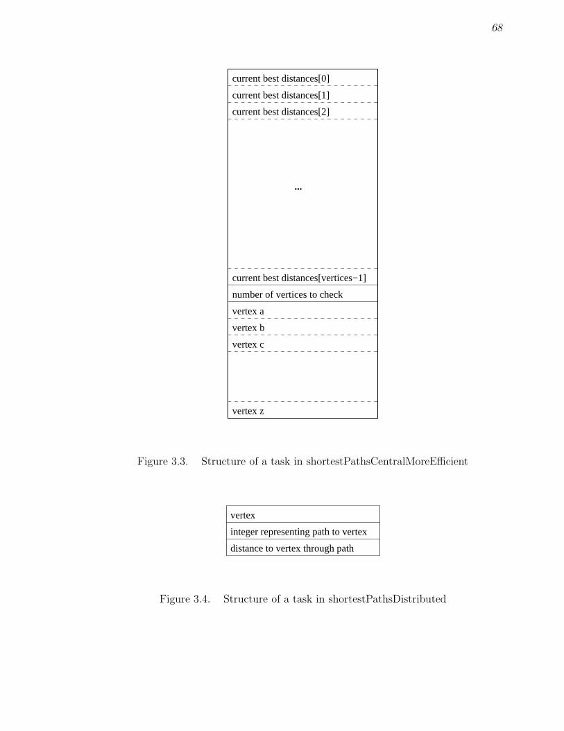
68
...
current best distances[0]
current best distances[1]
current best distances[2]
number of vertices to check
vertex a
vertex b
vertex c
vertex z
current best distances[vertices−1]
Figure 3.3. Structure of a task in shortestPathsCentralMoreEfficient
vertex
integer representing path to vertex
distance to vertex through path
Figure 3.4. Structure of a task in shortestPathsDistributed
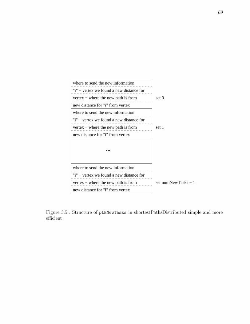
69
set 0
"i" − vertex we found a new distance for
vertex − where the new path is from
new distance for "i" from vertex
where to send the new information
set 1
"i" − vertex we found a new distance for
vertex − where the new path is from
new distance for "i" from vertex
where to send the new information
set numNewTasks − 1
"i" − vertex we found a new distance for
vertex − where the new path is from
new distance for "i" from vertex
where to send the new information
...
Figure 3.5.: Structure of ptkNewTasks in shortestPathsDistributed simple and moreefficient
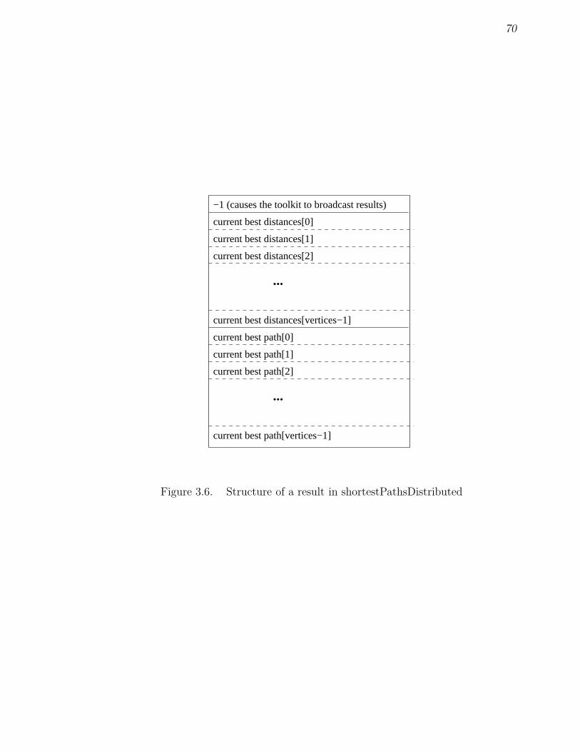
70
−1 (causes the toolkit to broadcast results)
current best path[0]
current best path[1]
current best path[2]
...
current best path[vertices−1]
current best distances[0]
current best distances[1]
current best distances[2]
...
current best distances[vertices−1]
Figure 3.6. Structure of a result in shortestPathsDistributed
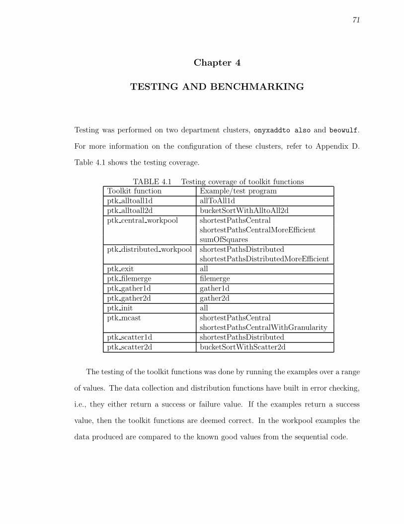
71
Chapter 4
TESTING AND BENCHMARKING
Testing was performed on two department clusters, onyxaddto also and beowulf.
For more information on the configuration of these clusters, refer to Appendix D.
Table 4.1 shows the testing coverage.
TABLE 4.1 Testing coverage of toolkit functionsToolkit function Example/test programptk alltoall1d allToAll1dptk alltoall2d bucketSortWithAlltoAll2dptk central workpool shortestPathsCentral
shortestPathsCentralMoreEfficientsumOfSquares
ptk distributed workpool shortestPathsDistributedshortestPathsDistributedMoreEfficient
ptk exit allptk filemerge filemergeptk gather1d gather1dptk gather2d gather2dptk init allptk mcast shortestPathsCentral
shortestPathsCentralWithGranularityptk scatter1d shortestPathsDistributedptk scatter2d bucketSortWithScatter2d
The testing of the toolkit functions was done by running the examples over a range
of values. The data collection and distribution functions have built in error checking,
i.e., they either return a success or failure value. If the examples return a success
value, then the toolkit functions are deemed correct. In the workpool examples the
data produced are compared to the known good values from the sequential code.
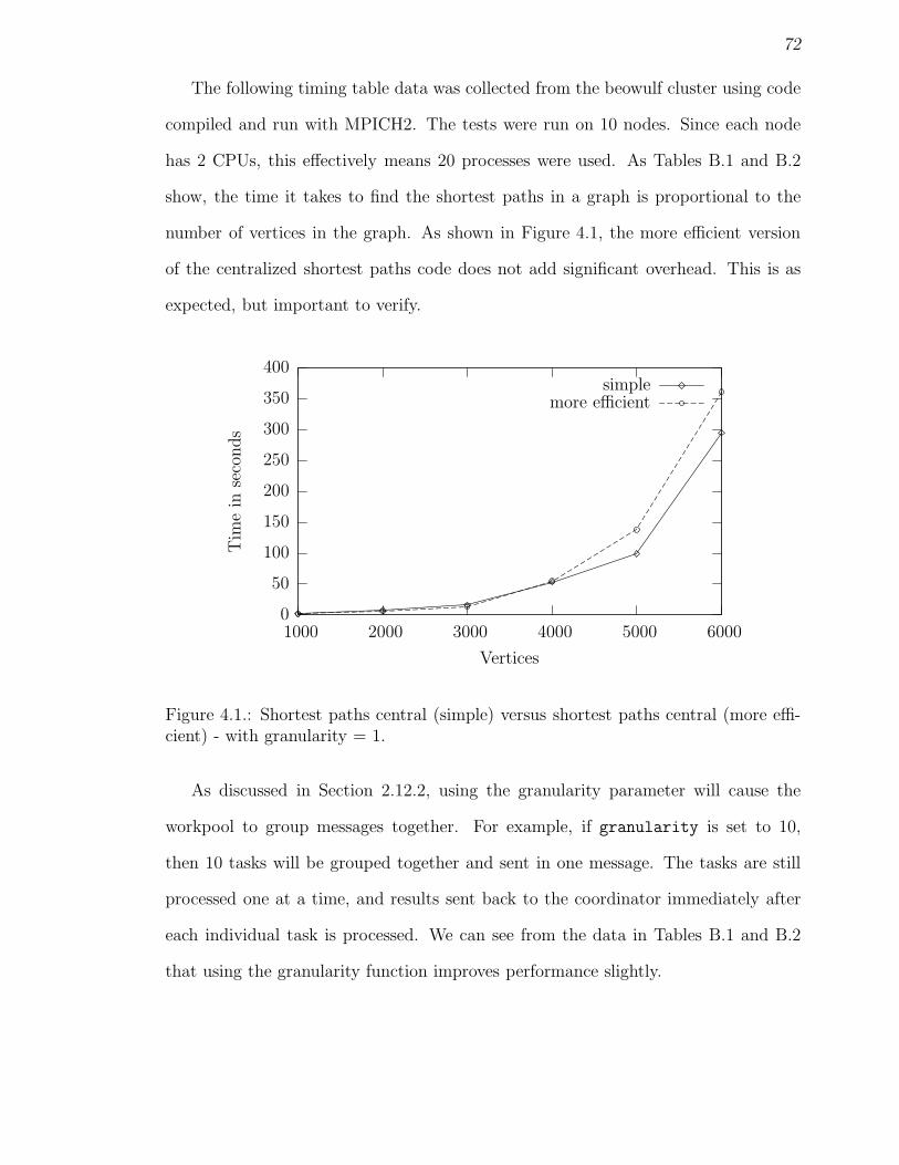
72
The following timing table data was collected from the beowulf cluster using code
compiled and run with MPICH2. The tests were run on 10 nodes. Since each node
has 2 CPUs, this effectively means 20 processes were used. As Tables B.1 and B.2
show, the time it takes to find the shortest paths in a graph is proportional to the
number of vertices in the graph. As shown in Figure 4.1, the more efficient version
of the centralized shortest paths code does not add significant overhead. This is as
expected, but important to verify.
0
50
100
150
200
250
300
350
400
1000 2000 3000 4000 5000 6000
Tim
ein
seco
nds
Vertices
simplemore efficient
Figure 4.1.: Shortest paths central (simple) versus shortest paths central (more effi-cient) - with granularity = 1.
As discussed in Section 2.12.2, using the granularity parameter will cause the
workpool to group messages together. For example, if granularity is set to 10,
then 10 tasks will be grouped together and sent in one message. The tasks are still
processed one at a time, and results sent back to the coordinator immediately after
each individual task is processed. We can see from the data in Tables B.1 and B.2
that using the granularity function improves performance slightly.
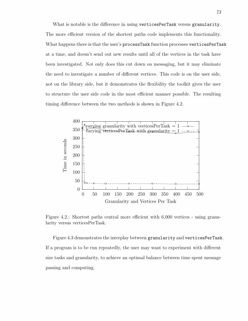
73
What is notable is the difference in using verticesPerTask versus granularity.
The more efficient version of the shortest paths code implements this functionality.
What happens there is that the user’s processTask function processes verticesPerTask
at a time, and doesn’t send out new results until all of the vertices in the task have
been investigated. Not only does this cut down on messaging, but it may eliminate
the need to investigate a number of different vertices. This code is on the user side,
not on the library side, but it demonstrates the flexibility the toolkit gives the user
to structure the user side code in the most efficient manner possible. The resulting
timing difference between the two methods is shown in Figure 4.2.
0
50
100
150
200
250
300
350
400
0 50 100 150 200 250 300 350 400 450 500
Tim
ein
seco
nds
Granularity and Vertices Per Task
varying granularity with verticesPerTask = 1varying verticesPerTask with granularity = 1
Figure 4.2.: Shortest paths central more efficient with 6,000 vertices - using granu-larity versus verticesPerTask.
Figure 4.3 demonstrates the interplay between granularity and verticesPerTask.
If a program is to be run repeatedly, the user may want to experiment with different
size tasks and granularity, to achieve an optimal balance between time spent message
passing and computing.
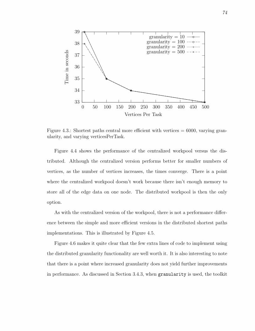
74
33
34
35
36
37
38
39
0 50 100 150 200 250 300 350 400 450 500
Tim
ein
seco
nds
Vertices Per Task
granularity = 10granularity = 100granularity = 200granularity = 500
Figure 4.3.: Shortest paths central more efficient with vertices = 6000, varying gran-ularity, and varying verticesPerTask.
Figure 4.4 shows the performance of the centralized workpool versus the dis-
tributed. Although the centralized version performs better for smaller numbers of
vertices, as the number of vertices increases, the times converge. There is a point
where the centralized workpool doesn’t work because there isn’t enough memory to
store all of the edge data on one node. The distributed workpool is then the only
option.
As with the centralized version of the workpool, there is not a performance differ-
ence between the simple and more efficient versions in the distributed shortest paths
implementations. This is illustrated by Figure 4.5.
Figure 4.6 makes it quite clear that the few extra lines of code to implement using
the distributed granularity functionality are well worth it. It is also interesting to note
that there is a point where increased granularity does not yield further improvements
in performance. As discussed in Section 3.4.3, when granularity is used, the toolkit
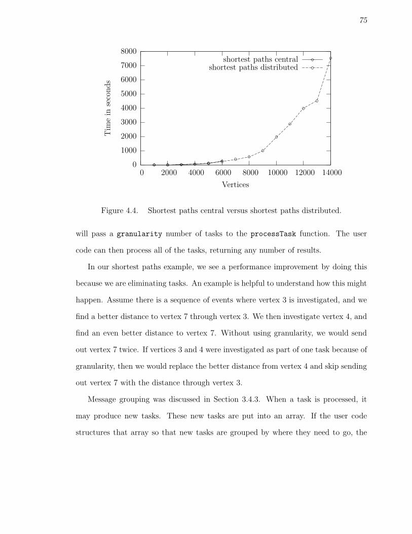
75
0
1000
2000
3000
4000
5000
6000
7000
8000
0 2000 4000 6000 8000 10000 12000 14000
Tim
ein
seco
nds
Vertices
shortest paths centralshortest paths distributed
Figure 4.4. Shortest paths central versus shortest paths distributed.
will pass a granularity number of tasks to the processTask function. The user
code can then process all of the tasks, returning any number of results.
In our shortest paths example, we see a performance improvement by doing this
because we are eliminating tasks. An example is helpful to understand how this might
happen. Assume there is a sequence of events where vertex 3 is investigated, and we
find a better distance to vertex 7 through vertex 3. We then investigate vertex 4, and
find an even better distance to vertex 7. Without using granularity, we would send
out vertex 7 twice. If vertices 3 and 4 were investigated as part of one task because of
granularity, then we would replace the better distance from vertex 4 and skip sending
out vertex 7 with the distance through vertex 3.
Message grouping was discussed in Section 3.4.3. When a task is processed, it
may produce new tasks. These new tasks are put into an array. If the user code
structures that array so that new tasks are grouped by where they need to go, the
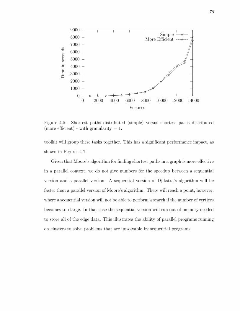
76
0
1000
2000
3000
4000
5000
6000
7000
8000
9000
0 2000 4000 6000 8000 10000 12000 14000
Tim
ein
seco
nds
Vertices
SimpleMore Efficient
Figure 4.5.: Shortest paths distributed (simple) versus shortest paths distributed(more efficient) - with granularity = 1.
toolkit will group these tasks together. This has a significant performance impact, as
shown in Figure 4.7.
Given that Moore’s algorithm for finding shortest paths in a graph is more effective
in a parallel context, we do not give numbers for the speedup between a sequential
version and a parallel version. A sequential version of Djikstra’s algorithm will be
faster than a parallel version of Moore’s algorithm. There will reach a point, however,
where a sequential version will not be able to perform a search if the number of vertices
becomes too large. In that case the sequential version will run out of memory needed
to store all of the edge data. This illustrates the ability of parallel programs running
on clusters to solve problems that are unsolvable by sequential programs.
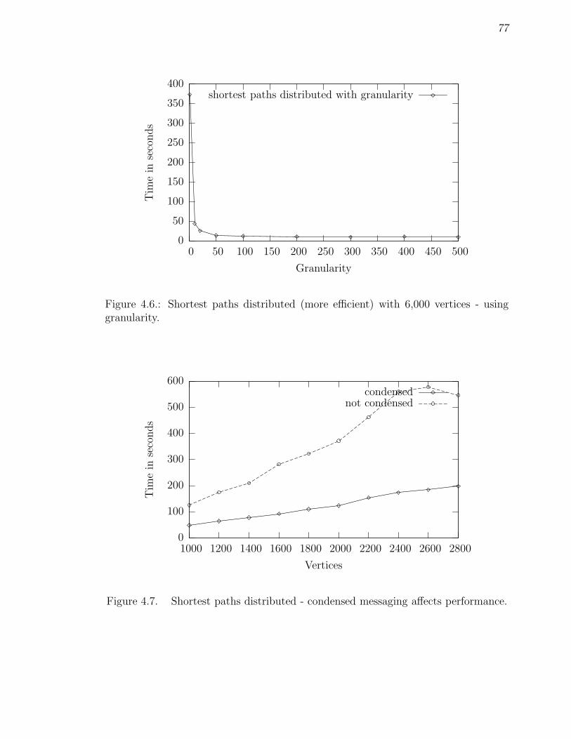
77
0
50
100
150
200
250
300
350
400
0 50 100 150 200 250 300 350 400 450 500
Tim
ein
seco
nds
Granularity
shortest paths distributed with granularity
Figure 4.6.: Shortest paths distributed (more efficient) with 6,000 vertices - usinggranularity.
0
100
200
300
400
500
600
1000 1200 1400 1600 1800 2000 2200 2400 2600 2800
Tim
ein
seco
nds
Vertices
condensednot condensed
Figure 4.7. Shortest paths distributed - condensed messaging affects performance.
78
Chapter 5
CONCLUSIONS
5.1 Library Support for Common Parallel Design Patterns
The Parallel Toolkit Library provides support for common design patterns used
throughout parallel programs. It includes both PVM and MPI versions. The ex-
amples given help users understand how to use the library functions.
The data sharing patterns of gather, scatter, and all to all are fully supported.
They allow users the flexibility of having odd amounts of data that are not evenly
divisible by the number of processes. The two-dimensional versions allow the user to
share “ragged” arrays of data. These elements are not provided by PVM or MPI.
The file merging functionality automates a common cluster task.
The workpools remove a significant layer of detail from writing workpool code.
The user of the workpool needs to provide the library with functions for processing
tasks and results. The library takes care of sending and receiving tasks and results.
Most importantly it handles termination detection, which can be quite cumbersome
to design and write.
The testing and benchmarking results are consistent with expectations. The li-
brary does not add a significant amount of overhead. In some cases, it may be more
efficient than code that users would write, because time may not be taken in non-
library code to incorporate some efficiencies that are part of the toolkit library.
79
5.2 General Observations and Reflections on Decisions Made
In a perfect parallel world, different program parameters would be evenly divisible
by other parameters. If this were the case, code would be much simpler to write.
If I would have imposed certain limitations on users of the library, and on my own
examples, the code would have taken much less time to write. However, it is my belief
that in the real world, numbers don’t always work out the way we might like them
to, thus the decision to add flexibility at the expense of complexity.
5.3 Potential Further Work
5.3.1 Centralized Workpool Queue
Creating a mechanism in the centralized workpool for pushing more urgent tasks to
the front of the queue might increase performance in certain applications. There is a
potential, however, as mentioned in Section 2.12.2, to slow down the workpool. This
would require an extra parameter somewhere, most likely the processTask function,
where new tasks that are created have a priority associated with them.
5.3.2 Multi-threading
Experimenting with multi-threading, particularly in the centralized workpool, would
be worth doing. There may be a bottleneck in the root being able to hand out tasks
quickly enough. Creating separate threads for communication and computation might
solve this problem. The decision was made to avoid any threading to make the code
as universal and portable as possible. Adding multi-threading may require a branch
in the “development tree.”

80
5.3.3 C++
It would be very interesting to try to create a C++ version of the library. The
workpools would lend themselves very nicely to object orientation. Instead of the
tasks being a collection of bytes, they could be objects.

81
REFERENCES
[1] Thomas H. Cormen, Charles E. Leiserson, Ronald L. Rivest, and Clifford Stein.Introduction to Algorithms. Second Edition, MIT Press, Cambridge, Massachus-sets, 2001.
[2] Edsger W. Dijkstra, W.H.J Feijen, A.J.M van Gasteren. “Derivation of a Termi-nation Detection Algorithm for a Distributed Computation.” Information Pro-cessing Letters, vol. 16(5), pp. 217-219.
[3] J.J. Dongarra, G.A. Geist, R.J. Mancheck, and P.M. Papadopou-los. “Adding context and static groups into PVM.” July 1995.http://www.epm.ornl.gov/pvm/context.ps.
[4] Al Geist, Adam Beguelin, Jack Dongarra, Weicheng Jiang, Robert Manchek,Vaidy Sunderam. PVM: Parallel Virtual Machine, A Users’ Guide and Tutorialfor Networked Parallel Computing. The MIT Press, Cambridge, Massachusetts,1994.
[5] William Gropp, Steven Huss-Lederman, Andrew Lumsdaine, Ewing Lusk, BillNitzberg, William Saphir, Marc Snir. MPI - The Complete Reference, Volume2, The MPI Extensions. The MIT Press, Cambridge, Massachusetts, 1998.
[6] William Gropp, Ewing Lusk, Anthony Skjellum. Using MPI: Portable Paral-lel Programming with the Message-Passing Interface. Second Edition, The MITPress, Cambridge, Massachusetts, 1999.
[7] Message Passing Interface. http://www-unix.mcs.anl.gov/mpi/.
[8] Jeff McGough. Personal communication. March 2007.
[9] Steffen Priebe. “Dynamic Task Generation and Transformation within a NestableWorkpool Skeleton.” European Conference on Parallel Computing (Euro-Par)2006, Dresden, Germany, LNCS 4128, Springer-Verlag, 2006.
[10] PVM: Parallel Virtual Machine. http://www.csm.ornl.gov/pvm/pvm home.html.
[11] N. Sachs, J. McGough. “Hybrid Process Farm/Work Pool Implementation in aDistributed Environment using MPI.” Conference Proceedings, Midwest Instruc-tional Computing Symposium. Duluth, Minnesota, April 2003.
82
[12] Marc Snir, Steve Otto, Steven Huss-Lederman, David Walker, Jack Dongarra.MPI - The Complete Reference, Volume 1, The MPI Core. Second Edition, TheMIT Press, Cambridge, Massachusetts, 1998.
[13] Barry Wilkinson, Michael Allen. Parallel Programming: Techniques and Appli-cations Using Networked Workstations and Parallel Computers. Second Edition,Pearson Prentice Hall, Upper Saddle River, New Jersey, 2005.
[14] Jason Man and Amit Jain. PRAND: A Parallel Random Number Generator.http://cs.boisestate.edu/~amit/research/prand.
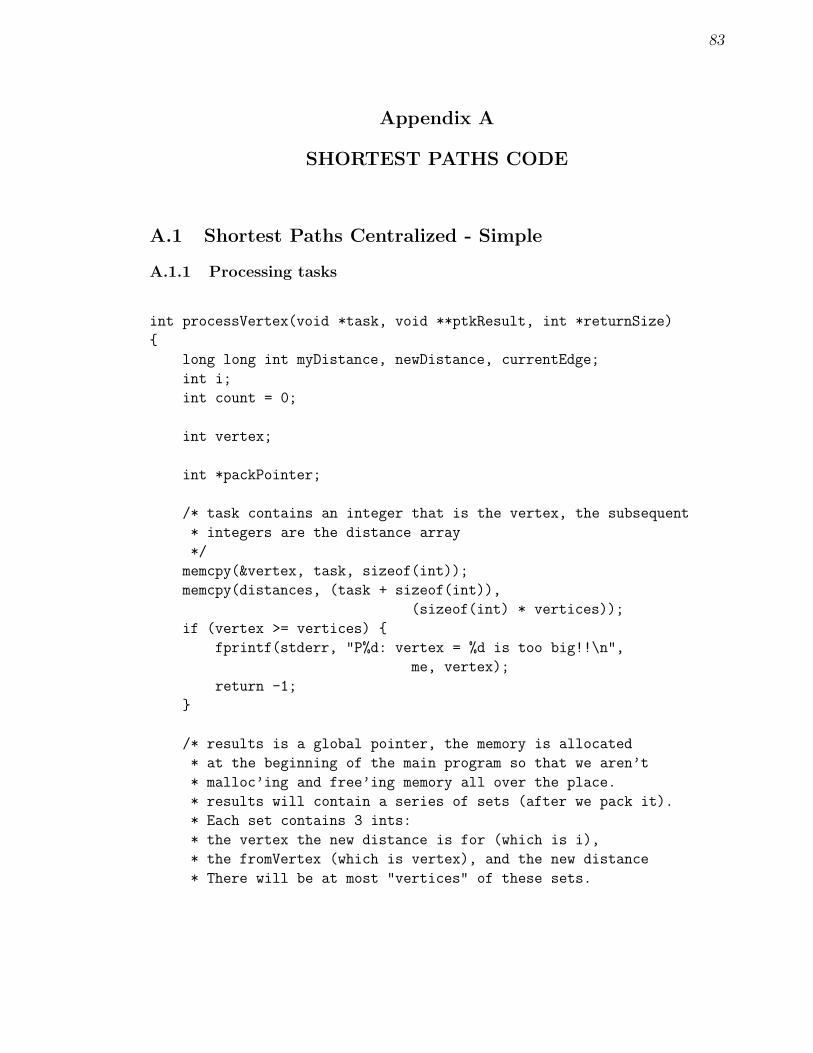
83
Appendix A
SHORTEST PATHS CODE
A.1 Shortest Paths Centralized - Simple
A.1.1 Processing tasks
int processVertex(void *task, void **ptkResult, int *returnSize)
{
long long int myDistance, newDistance, currentEdge;
int i;
int count = 0;
int vertex;
int *packPointer;
/* task contains an integer that is the vertex, the subsequent
* integers are the distance array
*/
memcpy(&vertex, task, sizeof(int));
memcpy(distances, (task + sizeof(int)),
(sizeof(int) * vertices));
if (vertex >= vertices) {
fprintf(stderr, "P%d: vertex = %d is too big!!\n",
me, vertex);
return -1;
}
/* results is a global pointer, the memory is allocated
* at the beginning of the main program so that we aren’t
* malloc’ing and free’ing memory all over the place.
* results will contain a series of sets (after we pack it).
* Each set contains 3 ints:
* the vertex the new distance is for (which is i),
* the fromVertex (which is vertex), and the new distance
* There will be at most "vertices" of these sets.

84
*/
packPointer = results;
/* save the first int of the result (packPointer)
* for the count
*/
packPointer++;
myDistance = distances[vertex];
for (i = 1; i < vertices; i++) {
currentEdge = edges[(vertex * vertices) + i];
if (currentEdge != RAND_MAX) {
newDistance = myDistance + currentEdge;
if (newDistance < distances[i]) {
memcpy(packPointer, &i, sizeof(int));
packPointer++;
memcpy(packPointer, &vertex, sizeof(int));
packPointer++;
memcpy(packPointer, &newDistance, sizeof(int));
packPointer++;
count++;
}
}
}
memcpy(results, &count, sizeof(int));
*ptkResult = results;
if (count > 0) {
*returnSize = (sizeof(int) * ((count * 3) + 1));
return ADD_RESULT;
}
else {
*returnSize = 0;
return DO_NOTHING;
}
}
A.1.2 Processing results
/* Coordinator function. Accepts a result, checks to see if the new
* distance is better than what we have so far.
85
*/
int processResult(void *results, void **ptkNewTasks, int *numNewTasks)
{
int *intResults;
int size;
int i;
int vertex;
int fromVertex;
int newDistance;
int *savePtr;
/* Results is an array of groups. Each group is a new
* ‘‘fromVertex’’ to put in the paths array,
* the vertex it is for, and the new distance to put in the
* distances array. Then we need to add the new vertices to
* the newTasks array. Using an int array to step through
* "results" makes some things easier.
*/
intResults = (int *)results;
memcpy(&size, intResults, sizeof(int));
intResults++;
*numNewTasks = 0;
for (i=0; i < size; i++) {
/* Extract the data */
memcpy(&vertex, intResults, sizeof(int));
intResults++;
memcpy(&fromVertex, intResults, sizeof(int));
intResults++;
memcpy(&newDistance, intResults, sizeof(int));
intResults++;
/* Is the newDistance better than what we have?? */
if (distances[vertex] > newDistance) {
paths[vertex] = fromVertex;
distances[vertex] = newDistance;
newInfo[vertex] = TRUE;
(*numNewTasks)++;
}
}
savePtr = newTasks;
86
/* Now we have to pack up the new tasks so
* that the coordinator can hand them out.
*/
for (i=0; i < vertices; i++) {
if (newInfo[i] == TRUE) {
memcpy(newTasks, &i, sizeof(int));
newTasks++;
memcpy(newTasks, distances, sizeof(int) * vertices);
newTasks += vertices;
}
newInfo[i] = FALSE;
}
*ptkNewTasks = savePtr;
newTasks = savePtr;
if (*numNewTasks > 0) {
return ADD_TASKS;
}
else {
return DO_NOTHING;
}
}
A.2 Shortest Paths Centralized - More Efficient
A.2.1 Processing tasks
/*
* Worker function. Accepts multiple vertices and tries to discover
* a shorter path to one of the other vertices
*/
int processVertex(void *dataToProcess, void **ptkResult,
int *returnSize)
{
long long int myDistance, newDistance, currentEdge;
int i, j;
int count = 0;
int vertex;
87
int verticesToCheck;
int *packPointer;
/* dataToProcess contains a distance array, then the
* number of vertices to investigate, then the
* vertices themselves.
*/
memcpy(distances, dataToProcess, (sizeof(int) * vertices));
memcpy(&verticesToCheck,
dataToProcess + (sizeof(int) * vertices),
sizeof(int));
for (i = 0; i < verticesToCheck; i++) {
memcpy(&vertex, dataToProcess +
(sizeof(int) * (vertices + 1 + i)),
sizeof(int));
myDistance = distances[vertex];
for (j = 1; j < vertices; j++) {
currentEdge = edges[(vertex * vertices) + j];
if (currentEdge != RAND_MAX) {
newDistance = myDistance + currentEdge;
if (newDistance < distances[j]) {
paths[j] = vertex;
distances[j] = newDistance;
if (newInfo[j] != TRUE) {
newInfo[j] = TRUE;
count++;
}
}
}
}
}
if (count > 0) {
/* result is a series of sets.
* Each set contains 3 ints:
* a fromVertex, the vertex, and the new distance
*/
*returnSize = (sizeof(int) * ((count * 3) + 1));
88
packPointer = result;
memcpy(packPointer, &count, sizeof(int));
packPointer++;
for (i=0; i < vertices; i++) {
if (newInfo[i] == TRUE) {
memcpy(packPointer, &paths[i], sizeof(int));
packPointer++;
memcpy(packPointer, &i, sizeof(int));
packPointer++;
memcpy(packPointer, &distances[i], sizeof(int));
packPointer++;
newInfo[i] = FALSE;
}
}
*ptkResult = result;
return ADD_RESULT;
}
else {
*returnSize = 0;
return DO_NOTHING;
}
}
A.2.2 Processing results
/* Coordinator function. Accepts a result, checks to see if the new
* distance is better than what we have so far.
*/
int processResult(void *results, void **ptkNewTasks, int *numNewTasks)
{
int *intResults;
int size;
int i;
int vertex;
int fromVertex;
int newDistance;
int *savePtr;
/* Results is an array of groups. Each group is a new
* ‘‘fromVertex’’ to put in the paths array,
89
* the vertex it is for, and the new distance to put in the
* distances array. Then we need to add the new vertices to
* the newTasks array. Using an int array to step through
* "results" makes some things easier.
*/
intResults = (int *)results;
memcpy(&size, intResults, sizeof(int));
intResults++;
*numNewTasks = 0;
for (i=0; i < size; i++) {
/* Extract the data */
memcpy(&vertex, intResults, sizeof(int));
intResults++;
memcpy(&fromVertex, intResults, sizeof(int));
intResults++;
memcpy(&newDistance, intResults, sizeof(int));
intResults++;
/* Is the newDistance better than what we have?? */
if (distances[vertex] > newDistance) {
paths[vertex] = fromVertex;
distances[vertex] = newDistance;
newInfo[vertex] = TRUE;
(*numNewTasks)++;
}
}
savePtr = newTasks;
/* Now we have to pack up the new tasks so
* that the coordinator can hand them out.
*/
if (count > 0) {
tail = count % verticesPerTask;
if (tail == 0) {
*numNewTasks = count / verticesPerTask;
}
else {
*numNewTasks = (count / verticesPerTask) + 1;
}
90
/* Each new task is the distance array, a count of how many
* vertices we are packing up, followed by up to N vertices,
* where N is indicated by the value of "verticesPerTask".
*/
newArray = newTasks;
for (i = 0; i < *numNewTasks; i++) {
/* First we copy in the current distances array, then the
* number of vertices we are packing
*/
memcpy(newArray, distances, (sizeof(int) * vertices));
newArray+= vertices;
/* If we’re on the last task, and count is not evenly
* divided by verticesPerTask, then we only pack a total
* of "tail" vertices
*/
if ((i == (*numNewTasks - 1)) && (tail != 0)) {
memcpy(newArray, &tail, sizeof(int));
newArray++;
j = 0;
count = 0;
while (count < tail) {
vertex = (i * verticesPerTask) + j;
if (newInfo[vertex] == TRUE) {
memcpy(newArray, &vertex, sizeof(int));
newArray++;
newInfo[vertex] = FALSE;
count++;
}
j++;
}
}
else {
memcpy(newArray, &verticesPerTask, sizeof(int));
newArray++;
j = 0;
count = 0;
while (count < verticesPerTask) {
vertex = (i * verticesPerTask) + j;
if (newInfo[vertex] == TRUE) {
91
memcpy(newArray, &vertex, sizeof(int));
newArray++;
newInfo[vertex] = FALSE;
count++;
}
j++;
}
}
}
*ptkNewTasks = newTasks;
return ADD_TASKS;
}
else {
*numNewTasks = 0;
return DO_NOTHING;
}
}
A.3 Shortest Paths Distributed - Simple
A.3.1 Processing tasks
/*
* Worker function. Accepts a vertex number and tries to discover
* a shorter path to one of the other vertices
*/
void *processVertex(void *task, int tasksToProcess,
void **ptkNewTasks, int *numNewTasks,
void **ptkResults, int *numResults)
{
long long int myDistance, newDistance, currentEdge;
int i;
int count = 0;
int sendTo;
int vertex;
int fromVertex;
int distance;
int *intPointer;
int minusOne = -1;
/* Make dataToProcess a little easier to use */
92
int *data = (int *)task;
/* task contains the sendTo (which we ignore here),
* a vertex, a fromVertex, and a distance
* This version of the code assumes a granularity of 1,
* so we ignore the tasksToProcess number.
*/
vertex = data[1];
fromVertex = data[2];
distance = data[3];
/* ptkNewTasks is a series of 4 ints for a maximum of
* n vertices - each is where to send the new task,
* the fromVertex, the vertex the new distance is for,
* and the new distance.
*/
intPointer = newTasks;
myDistance = distances[vertex];
for (i = 1; i < vertices; i++) {
currentEdge =
myedges[((vertex - myFirstVertex) * vertices) + i];
if (currentEdge != RAND_MAX) {
newDistance = myDistance + currentEdge;
if (newDistance < distances[i]) {
/* The math gets a little hairy here in
* order to account for the case where vertices
* are not evenly divided by group size
*/
sendTo = i * gsize / (vertices - (vertices % gsize));
if (sendTo == gsize) {
sendTo = gsize - 1;
}
distances[i] = newDistance;
paths[i] = vertex;
memcpy(intPointer, &sendTo, sizeof(int));
intPointer++;
memcpy(intPointer, &i, sizeof(int));
intPointer++;
93
memcpy(intPointer, &vertex, sizeof(int));
intPointer++;
memcpy(intPointer, &newDistance, sizeof(int));
intPointer++;
count++;
}
}
}
if (count > 0) {
*numTasks = count;
/* The first value in the results array is where to send
* the info. The size in this case is the length of the
* distance array (vertices) plus the length of the paths
* array (vertices) plus where to send the result, which
* is -1, meaning send to everyone.
*/
memcpy(results, &minusOne, sizeof(int));
memcpy(results + 1, distances, sizeof(int) * vertices);
memcpy(results + vertices + 1, paths, sizeof(int) * vertices);
*numResults = 1;
*ptkNewTasks = newTasks;
*ptkResults = results;
}
else {
*numTasks = 0;
*numResults = 0;
}
return (void *)1;
}
A.3.2 Processing results
void *processResult(void *result)
{
int i;
int *data;
/* The first integer is the sendTo that we packed in
* processVertex. The subsequent "vertices" elements
* are the distances, and the next "vertices" elements
94
* are the paths.
*/
data = (int *)result;
data++;
for (i = 0; i < vertices; i++) {
if (data[i] < distances[i]) {
memcpy(&(distances[i]), result + (i * sizeof(int)),
sizeof(int));
memcpy(&(paths[i]), result + ((i + vertices) * sizeof(int)),
sizeof(int));
}
}
return (void *)1;
}
A.4 Shortest Paths Distributed - More Efficient
A.4.1 Processing tasks
/*
* Worker function. Accepts multiple vertices (the quantity of
* which is defined by the "granularity" variable) and tries
* to discover a shorter path to one of the other vertices
*/
void *processVertex(void *dataToProcess, int tasksToProcess,
void **ptkNewTasks, int *numNewTasks,
void **ptkResults, int *numResults)
{
long long int myDistance, newDistance, currentEdge;
int i, j;
int count = 0;
int sendTo;
int vertex;
int fromVertex;
int distance;
int *intPointer;
int *data;
int minusOne = -1;
/* This make the code a bit more readable */
95
data = (int *)dataToProcess;
for (i = 0; i < tasksToProcess; i++) {
/* The workpool sends tasks just like what we pack when
* we create new objects. We ignore the ‘‘sendTo’’
* integer that is at the beginning of each task.
*/
vertex = data[(i * 3) + 1];
fromVertex = data[(i * 3) + 2];
distance = data[(i * 3) + 3];
myDistance = distances[vertex];
for (j = 1; j < vertices; j++) {
currentEdge =
myedges[((vertex - myFirstVertex) * vertices) + j];
if (currentEdge != RAND_MAX) {
newDistance = myDistance + currentEdge;
if (newDistance < distances[j]) {
distances[j] = newDistance;
paths[j] = vertex;
if (newInfo[j] != TRUE) {
newInfo[j] = TRUE;
count++;
}
}
}
}
}
if (count > 0) {
*numNewTasks = count;
/* newTasks is a series of 4 ints for a maximum of
* n vertices - each is where to send the new task,
* the fromVertex, the vertex the new distance is for,
* and the new distance
*/
intPointer = newTasks;
for (j = 0; j < vertices; j++) {
if (newInfo[j] == TRUE) {
96
/* The math gets a little hairy here in order to
* account for the case where vertices are not
* evenly divided by group size. Note that the
* placement of the parentheses is important.
*/
sendTo = j * gsize / (vertices - (vertices % gsize));
if (sendTo == gsize) {
sendTo = gsize - 1;
}
memcpy(intPointer, &sendTo, sizeof(int));
intPointer++;
memcpy(intPointer, &j, sizeof(int));
intPointer++;
memcpy(intPointer, &paths[j], sizeof(int));
intPointer++;
memcpy(intPointer, &distances[j], sizeof(int));
intPointer++;
}
newInfo[j] = FALSE;
}
/* The first value in the results array is where to send
* the info. The size in this case is the length of the
* distance array (vertices) plus the length of the paths
* array (vertices) plus where to send the result,
* which is -1, meaning send to everyone.
*/
memcpy(results, &minusOne, sizeof(int));
memcpy(results + 1, distances, sizeof(int) * vertices);
memcpy(results + vertices + 1, paths, sizeof(int) * vertices);
*numResults = 1;
*ptkNewTasks = newTasks;
*ptkResults = results;
}
else {
*numNewTasks = 0;
*numResults = 0;
}
return (void *)1;
}

97
A.4.2 Processing results
This function is the same as in Shortest Paths Distributed, the simple version.
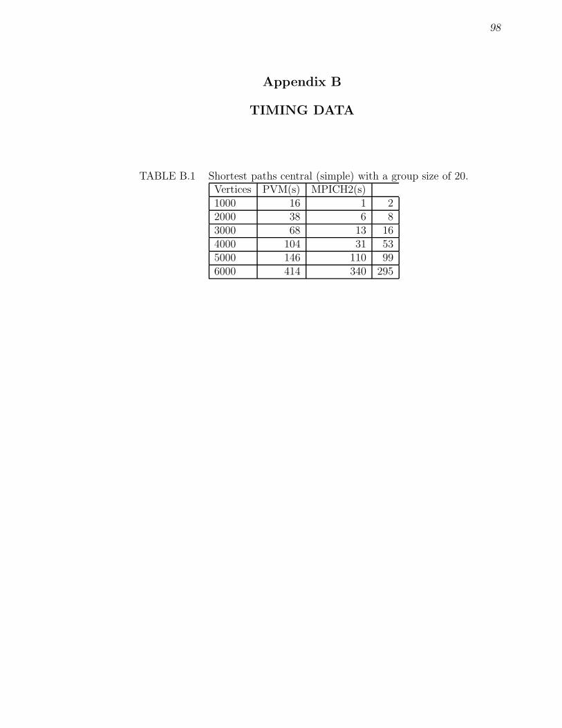
98
Appendix B
TIMING DATA
TABLE B.1 Shortest paths central (simple) with a group size of 20.Vertices PVM(s) MPICH2(s)1000 16 1 22000 38 6 83000 68 13 164000 104 31 535000 146 110 996000 414 340 295
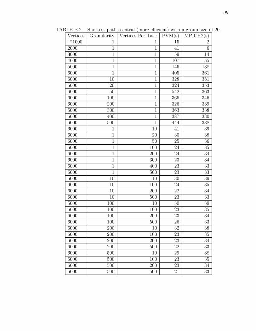
99
TABLE B.2 Shortest paths central (more efficient) with a group size of 20.Vertices Granularity Vertices Per Task PVM(s) MPICH2(s)””1000 1 1 15 22000 1 1 41 63000 1 1 59 144000 1 1 107 555000 1 1 146 1386000 1 1 405 3616000 10 1 328 3816000 20 1 324 3536000 50 1 542 3636000 100 1 366 3466000 200 1 326 3396000 300 1 363 3386000 400 1 387 3306000 500 1 444 3386000 1 10 41 396000 1 20 30 386000 1 50 25 366000 1 100 24 356000 1 200 24 346000 1 300 23 346000 1 400 23 336000 1 500 23 336000 10 10 30 396000 10 100 24 356000 10 200 22 346000 10 500 23 336000 100 10 30 396000 100 100 23 356000 100 200 23 346000 100 500 26 336000 200 10 32 386000 200 100 23 356000 200 200 23 346000 200 500 22 336000 500 10 29 386000 500 100 23 356000 500 200 23 346000 500 500 21 33
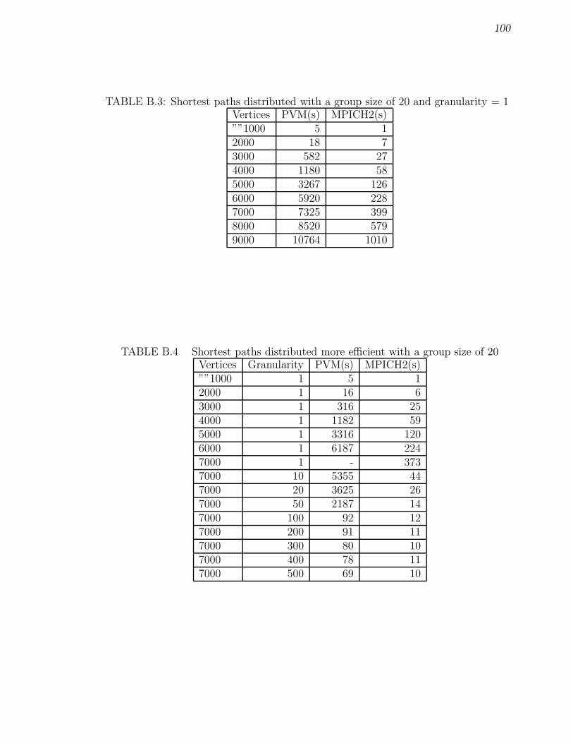
100
TABLE B.3: Shortest paths distributed with a group size of 20 and granularity = 1Vertices PVM(s) MPICH2(s)””1000 5 12000 18 73000 582 274000 1180 585000 3267 1266000 5920 2287000 7325 3998000 8520 5799000 10764 1010
TABLE B.4 Shortest paths distributed more efficient with a group size of 20Vertices Granularity PVM(s) MPICH2(s)””1000 1 5 12000 1 16 63000 1 316 254000 1 1182 595000 1 3316 1206000 1 6187 2247000 1 - 3737000 10 5355 447000 20 3625 267000 50 2187 147000 100 92 127000 200 91 117000 300 80 107000 400 78 117000 500 69 10
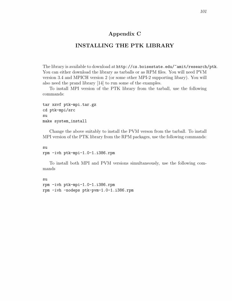
101
Appendix C
INSTALLING THE PTK LIBRARY
The library is available to download at http://cs.boisestate.edu/~amit/research/ptk.You can either download the library as tarballs or as RPM files. You will need PVMversion 3.4 and MPICH version 2 (or some other MPI-2 supporting libary). You willalso need the prand library [14] to run some of the examples.
To install MPI version of the PTK library from the tarball, use the followingcommands:
tar xzvf ptk-mpi.tar.gz
cd ptk-mpi/src
su
make system_install
Change the above suitably to install the PVM verson from the tarball. To installMPI version of the PTK library from the RPM packages, use the following commands:
su
rpm -ivh ptk-mpi-1.0-1.i386.rpm
To install both MPI and PVM versions simultaneously, use the following com-mands
su
rpm -ivh ptk-mpi-1.0-1.i386.rpm
rpm -ivh -nodeps ptk-pvm-1.0-1.i386.rpm

102
Appendix D
BOISE STATE COMPUTER SCIENCE DEPARTMENTCLUSTERS
D.1 Onyx
Onyx is the cluster used by students taking Computer Science courses. It’s vitalsinclude,
• a head node with dual 3.2GHz Intel Xeon processors with 4GB RAM,
• nodes 01-27: 2.8GHz Intel Pentium 4 w/HT processors with 1GB RAM,
• nodes 28-32: 3.2GHz Intel Pentium 4 w/HT processors with 1GB RAM,
• private gigabit ethernet,
• runs Fedora Core 5, kernel 2.6.16,
• compiles code with gcc version 4.1.1.
D.2 Beowulf
Beowulf, aka “The Big Cluster,”
• has a head node with dual 2.4GHz Intel Xeon processors with 4GB RAM,
• 60 dual-processor nodes with dual 2.4GHz Intel Xeon processors with 1GBRAM,
• private gigabit ethernet,
• runs Fedora Core 3, kernel 2.6.12,
• compiles code with gcc version 3.4.4.