Proton-proton scattering from low to LHC-energiesfolk.uio.no/finnr/talks/pp-scattering.pdf · Proton-proton scattering from low to LHC-energies • Coulomb scattering • Low-energy

Proton-proton scattering from low to LHC-energies

• Coulomb scattering

• Low-energy strong interactions

• Regge poles and the pomeron

• The Froissart bound

• Feynman parton model

• Recent ideas and conclusion

Finn Ravndal, Dept of Physics, UiO

HEP-coll, 13/11 - 2009

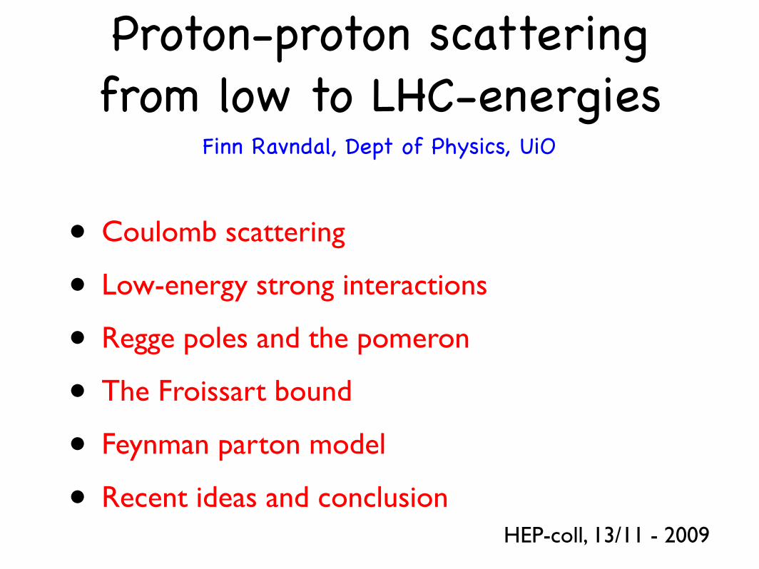
Coulomb scattering

e

e

Q Q2= 4p2

sin2 !/2

in CM-frame:

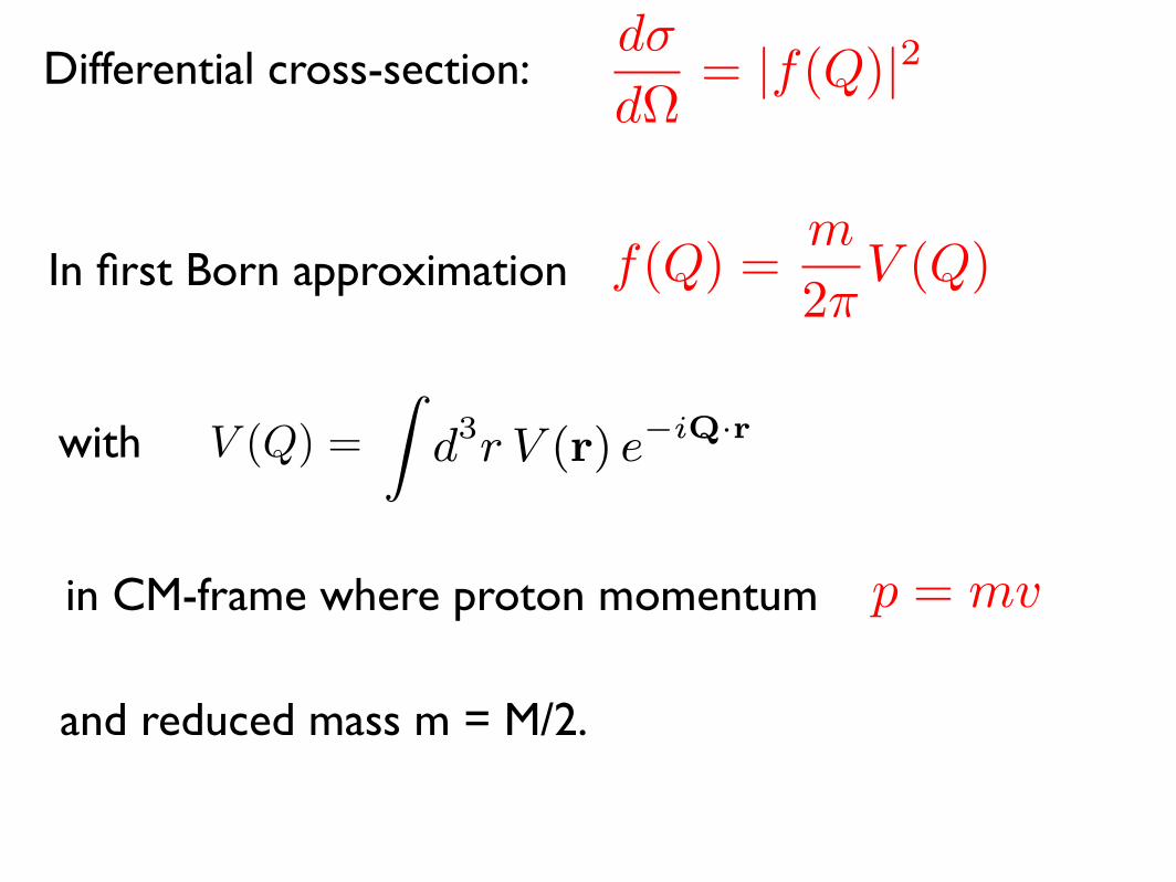
Differential cross-section:

In first Born approximation

in CM-frame where proton momentum

d!

d!= |f(Q)|2

f(Q) =m

2!V (Q)

with

becomes infinite Born series

T = V + V G0V + V G0V G0V + · · ·

when expressed by the free Green’s function

G0(E) =1

E ! H0 + i!

First Born approximation

T (1)p!p

= "p! |bV |p# =

Zd3r V (r) e"iQ·r

Scattering on potential of finite range R

V(r)

rR

at low energies p ! 1/R:

d"d!

= a20

where S-wave scattering length

a0 =M

4#

Zd3r V (r)

in this approximation.

3

V (Q) =

and reduced mass m = M/2.

p = mv

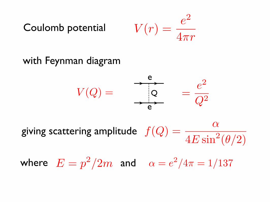
Coulomb potential

with Feynman diagram

= + + + ! ! !

+=

Figure 6: Coulomb propagator as an infinite sum.

or Kummer function M(a, b;x)[23]. For the repulsive Coulomb potential VC = !/r thein-state solution with outgoing spherical waves in the future is

"(+)p (r) = e!

1

2!"!(1 + i#)M(!i#, 1; ipr ! ip · r) eip·r (20)

The corresponding out-state has incoming spherical waves in the distant past and is givenby the wavefunction

"(!)p (r) = e!

1

2!"!(1 ! i#)M(i#, 1;!ipr ! ip · r) eip·r (21)

where # = !M/2p is the parameter which also appeared in the earlier perturbative calcu-lation. The probability to find the two protons at zero separation is thus

C2" " |"(±)

p (0)|2 = e!!"!(1 + i#)!(1 ! i#) =2$#

e2!" ! 1(22)

which is the well-known Sommerfeld factor[23][24]. When the relative velocity betweenthe particles goes to zero, it becomes exponentially small. At higher velocities # < 1 andthe Coulomb repulsion is perturbative. We then recover to lowest order the result 1 ! $#obtained from the Feynman diagram Fig. 4 in the previous section.

With these Coulomb eigenstates we can now find a more useful expression for theGreen’s functions (18). Since the scattering states form a complete set in the repulsivecase we consider here, we can instead write it as in (17). Taking the matrix element incoordinate space, we then have for the retarded function

#r" | !G(+)C |r$ = M

"d3q

(2$)3"(+)

q (r")"(+)#q (r)

p2 ! q2 + i%(23)

In the next section we will see that this propagator gives the main part of the non-perturbative Coulomb corrections of the strong scattering amplitude.

9

giving scattering amplitude

and ! = e2/4" = 1/137where

V (r) =e2

4!r

Q

e

e

=

e2

Q2V (Q) =

f(Q) =!

4E sin2("/2)

E = p2/2m

= + + + ! ! !

+=

Figure 6: Coulomb propagator as an infinite sum.

or Kummer function M(a, b;x)[23]. For the repulsive Coulomb potential VC = !/r thein-state solution with outgoing spherical waves in the future is

"(+)p (r) = e!

1

2!"!(1 + i#)M(!i#, 1; ipr ! ip · r) eip·r (20)

The corresponding out-state has incoming spherical waves in the distant past and is givenby the wavefunction

"(!)p (r) = e!

1

2!"!(1 ! i#)M(i#, 1;!ipr ! ip · r) eip·r (21)

where # = !M/2p is the parameter which also appeared in the earlier perturbative calcu-lation. The probability to find the two protons at zero separation is thus

C2" " |"(±)

p (0)|2 = e!!"!(1 + i#)!(1 ! i#) =2$#

e2!" ! 1(22)

which is the well-known Sommerfeld factor[23][24]. When the relative velocity betweenthe particles goes to zero, it becomes exponentially small. At higher velocities # < 1 andthe Coulomb repulsion is perturbative. We then recover to lowest order the result 1 ! $#obtained from the Feynman diagram Fig. 4 in the previous section.

With these Coulomb eigenstates we can now find a more useful expression for theGreen’s functions (18). Since the scattering states form a complete set in the repulsivecase we consider here, we can instead write it as in (17). Taking the matrix element incoordinate space, we then have for the retarded function

#r" | !G(+)C |r$ = M

"d3q

(2$)3"(+)

q (r")"(+)#q (r)

p2 ! q2 + i%(23)

In the next section we will see that this propagator gives the main part of the non-perturbative Coulomb corrections of the strong scattering amplitude.

9

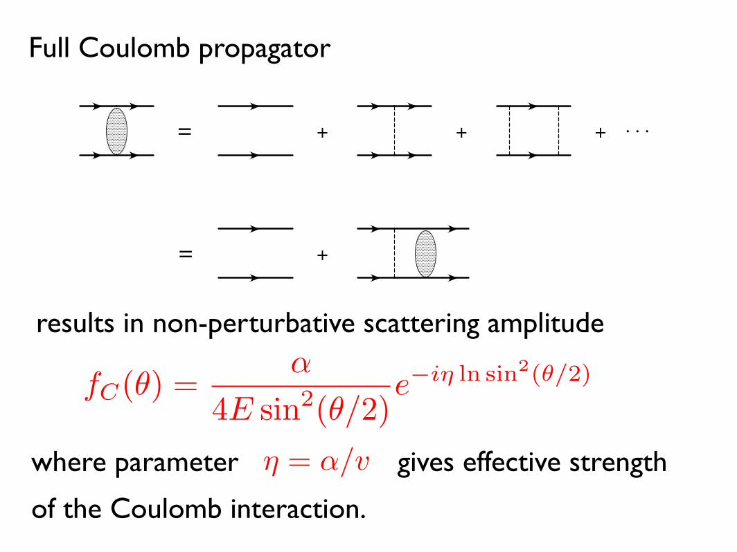
Full Coulomb propagator

results in non-perturbative scattering amplitude

where parameter ! = "/v gives effective strength

of the Coulomb interaction.

fC(!) ="

4E sin2(!/2)e!iη ln sin2(θ/2)

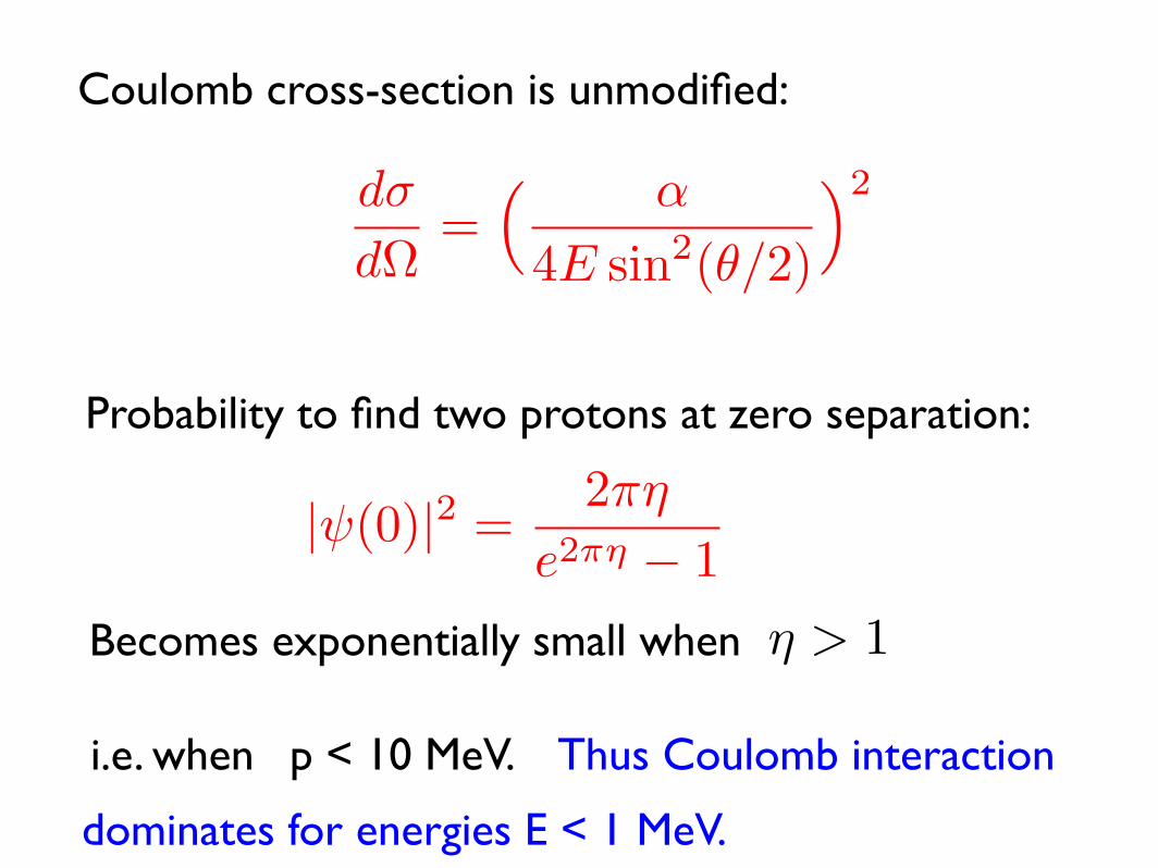
Probability to find two protons at zero separation:

|!(0)|2 =2"#

e2!" ! 1

Becomes exponentially small when ! > 1

i.e. when p < 10 MeV.

Coulomb cross-section is unmodified:

d!

d!=

! "

4E sin2(#/2)

"2

Thus Coulomb interaction

dominates for energies E < 1 MeV.

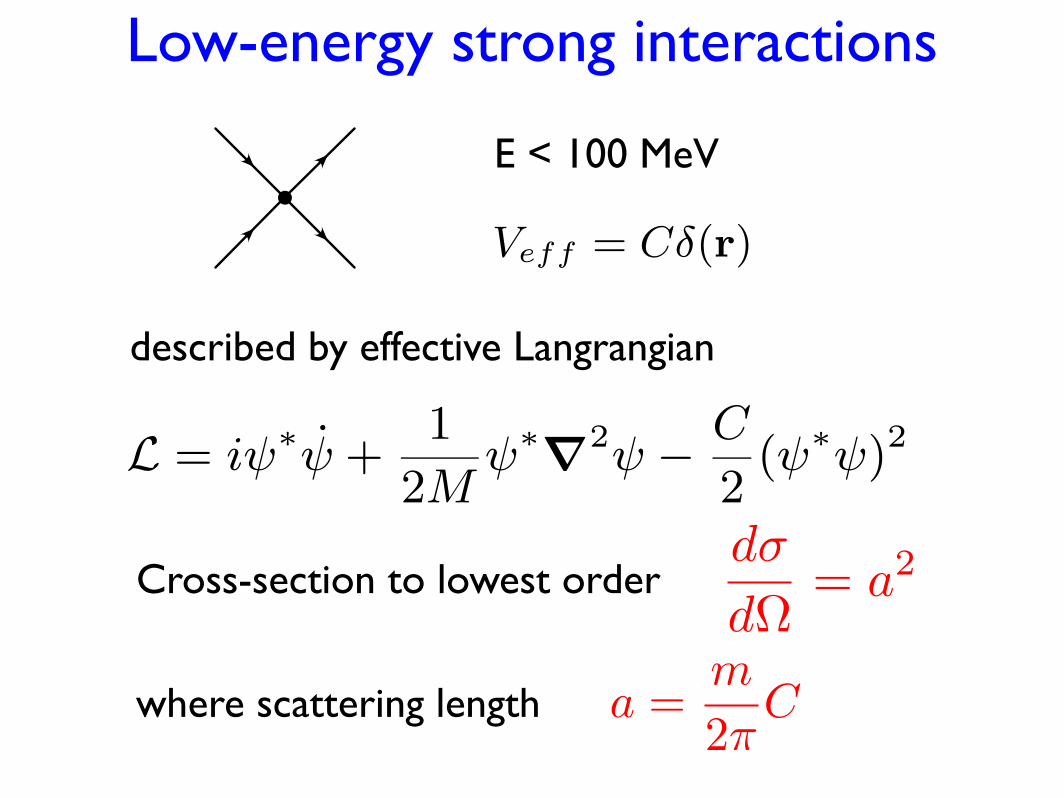
Low-energy strong interactions

E!ective potential, valid at low energies:

Veff = C!(r)

where coupling constant C = 4!M

a in first Born

approximation.

Higher order Born corrections can now be obtained ine!ective field theory

L = i"!" +1

2M"!

!2" ! C

2("!")2

using standard field-theoretic perturbation theory withnon-relativistic propagator

G0(E,p) =1

E ! p2/2M + i#

and elementary vertex

Second order Born correction from Feynman diagram

4


Veff = C!(r)


a in first Born

approximation.


L = i"!" +1

2M"!

!2" ! C

2("!")2


G0(E,p) =1

E ! p2/2M + i#



4

Cross-section to lowest order


Veff = C!(r)


a in first Born

approximation.


L = i"!" +1

2M"!

!2" ! C

2("!")2


G0(E,p) =1

E ! p2/2M + i#



4

described by effective Langrangian

d!

d!= a

2

where scattering length a =m

2!C

E < 100 MeV

Higher order corrections

with value C2I0(p) with bubble integral

I0(p) =

Zd3k

(2!)32M

p2 ! k2 + i"

Higher order diagram with n bubbles

...

gives similarly Cn+1In0 (p). Total scattering amplitude:

T (p) = Cˆ1 + CI0 + (CI0)

2 + (CI0)3 + · · ·

˜

=C

1 ! CI0=

11/C ! I0(p)

Bubble integral I0(p) is divergent in d = 3 dimensions.Regularize with cut-o! ! " 1/R giving

I0(p) = ! M2!2

„! +

i2!p

«

which implies that bare coupling C = C(!).

5


I0(p) =

Zd3k

(2!)32M

p2 ! k2 + i"


...


T (p) = Cˆ1 + CI0 + (CI0)

2 + (CI0)3 + · · ·

˜

=C

1 ! CI0=

11/C ! I0(p)


I0(p) = ! M2!2

„! +

i2!p

«


5

+ ...... + + ....

given by bubble integral


I0(p) =

Zd3k

(2!)32M

p2 ! k2 + i"


...


T (p) = Cˆ1 + CI0 + (CI0)

2 + (CI0)3 + · · ·

˜

=C

1 ! CI0=

11/C ! I0(p)


I0(p) = ! M2!2

„! +

i2!p

«


5


I0(p) =

Zd3k

(2!)32M

p2 ! k2 + i"


...


T (p) = Cˆ1 + CI0 + (CI0)

2 + (CI0)3 + · · ·

˜

=C

1 ! CI0=

11/C ! I0(p)


I0(p) = ! M2!2

„! +

i2!p

«


5

Full scattering amplitude:

T

Bubble integral with cut-off regularization:


I0(p) =

Zd3k

(2!)32M

p2 ! k2 + i"


...


T (p) = Cˆ1 + CI0 + (CI0)

2 + (CI0)3 + · · ·

˜

=C

1 ! CI0=

11/C ! I0(p)


I0(p) = ! M2!2

„! +

i2!p

«


5

Remove cut-off ! by introducing renormalizedcoupling constant

Renormalization

Remove cut-o! ! by introducing renormalized couplingconstant

1CR

=1C

+M!2!2

with value CR = 4!M

a which gives scattering amplitude

T (p) =4!

M

1

1/a + ip

and is now unitary. Di!erential cross-section

d"

d"=

a2

1 + (ap)2

Renormalized coupling CR goes to zero as ! ! ", no scattering

on !-function potential in this limit. Theory is then trivial.

Instead of cut-o! regularization, dimensionalregularization was introduced by Kaplan, Savage andWise (1998) by the name PDS giving

I0(p) =“µ

2

”"Z

ddk

(2!)d

2M

p2 ! k2 + i#

= !M

4!

`µ + ip

´

where d = 3 ! # after subtracting pole at d = 2, i.e.

Power Divergence Subtraction.

Comparing with cut-o!: µ " !.

6

Thus

Renormalization


1CR

=1C

+M!2!2

with value CR = 4!M


T (p) =4!

M

1

1/a + ip


d"

d"=

a2

1 + (ap)2




I0(p) =“µ

2

”"Z

ddk

(2!)d

2M

p2 ! k2 + i#

= !M

4!

`µ + ip

´




6

T with a =M

4!CR

and differential cross-section becomes

Renormalization


1CR

=1C

+M!2!2

with value CR = 4!M


T (p) =4!

M

1

1/a + ip


d"

d"=

a2

1 + (ap)2




I0(p) =“µ

2

”"Z

ddk

(2!)d

2M

p2 ! k2 + i#

= !M

4!

`µ + ip

´




6

Renormalization


1CR

=1C

+M!2!2

with value CR = 4!M


T (p) =4!

M

1

1/a + ip


d"

d"=

a2

1 + (ap)2




I0(p) =“µ

2

”"Z

ddk

(2!)d

2M

p2 ! k2 + i#

= !M

4!

`µ + ip

´




6

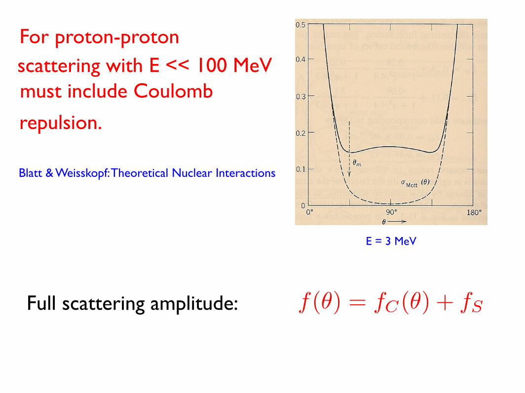
must include Coulomb

repulsion.

Blatt & Weisskopf: Theoretical Nuclear Interactions

Full scattering amplitude: f(!) = fC(!) + fS

For proton-protonscattering with E << 100 MeV

E = 3 MeV

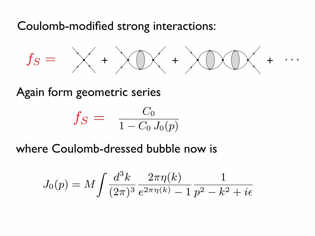
Coulomb-modified strong interactions:Strong interactions now modified by Coulomb e!ects

+ + + ! ! !

with Coulomb-dressed strong interaction bubble J0(p):

= + + + ! ! !

All such Feynman diagrams again form geometric seriesgiving scattering amplitude

TSC(p) = C2!

C0

1 ! C0 J0(p)

Gives Coulomb-modified scattering length

1aC

=4!M

1TSC(p)

! "MH(#)

where standard function

H(#) = $(i#) +1

2i#! log(i#)

Experimentally aC = !7.82 fm compared with

apn " ann " !20 fm.

Now calculate aC from above TSC(p):

11

fS =

Again form geometric series

Strong interactions now modified by Coulomb e!ects

+ + + ! ! !

with Coulomb-dressed strong interaction bubble J0(p):

= + + + ! ! !

All such Feynman diagrams again form geometric seriesgiving scattering amplitude

TSC(p) = C2!

C0

1 ! C0 J0(p)


1aC

=4!M

1TSC(p)

! "MH(#)

where standard function

H(#) = $(i#) +1

2i#! log(i#)

Experimentally aC = !7.82 fm compared with

apn " ann " !20 fm.

Now calculate aC from above TSC(p):

11

fS =

where Coulomb-dressed bubble now is

Coulomb-dressed bubble J0(p) is amplitude for protonsto move from zero separation back to zero separation,i.e. J0(p) = GC(E; r! = 0, r = 0) or

J0(p) = M

Zd3k

(2!)32!"(k)

e2!"(k) ! 1

1p2 ! k2 + i#

Can be done analytically (!):

J0(p) =$M2

4!

»1#

+ lnµ"

!$M

+ 1 ! 32CE

–

! µM4!

! $M2

4!H(")

with Euler constant CE = 0.5772 . . ..


1aC

=1

a(µ)! $M

»ln

µ"

!$M

+ 1 ! 32CE

–

when divergence 1/# is absorbed in strong interactioncoupling

C0(µ) =4!

M

1

1/a(µ) ! µ

Expect a(µ) # apn # !20 fm for µ # ! # m!.

Relation between scattering lengths first derived byBlatt and Jackson (1950) in potential model:

1aC

=1

app! $M

»ln

1$Mr0

! 0.33

–

12

Can be done analytically

and gives Coulomb-modified scattering length:

Kong and Ravndal (1998)

Coulomb-dressed bubble J0(p) is amplitude for protonsto move from zero separation back to zero separation,i.e. J0(p) = GC(E; r! = 0, r = 0) or

J0(p) = M

Zd3k

(2!)32!"(k)

e2!"(k) ! 1

1p2 ! k2 + i#

Can be done analytically (!):

J0(p) =$M2

4!

»1#

+ lnµ"

!$M

+ 1 ! 32CE

–

! µM4!

! $M2

4!H(")

with Euler constant CE = 0.5772 . . ..


1aC

=1

a(µ)! $M

»ln

µ"

!$M

+ 1 ! 32CE

–

when divergence 1/# is absorbed in strong interactioncoupling

C0(µ) =4!

M

1

1/a(µ) ! µ

Expect a(µ) # apn # !20 fm for µ # ! # m!.

Relation between scattering lengths first derived byBlatt and Jackson (1950) in potential model:

1aC

=1

app! $M

»ln

1$Mr0

! 0.33

–

12

Blatt and Jackson (1950)

from quantum mechanics in a potential model.

Proton-proton fusion:

Low-energy pp scattering and fusion:

A modern approach

Finn Ravndal, University of Oslo

• Scattering on a !-function potential

• Renormalization

• Proton-neutron scattering and the deuteron D

• Proton-proton scattering and Coulomb e!ects

• Solar fusion p + p ! D + e+ + "e

• Conclusion

1

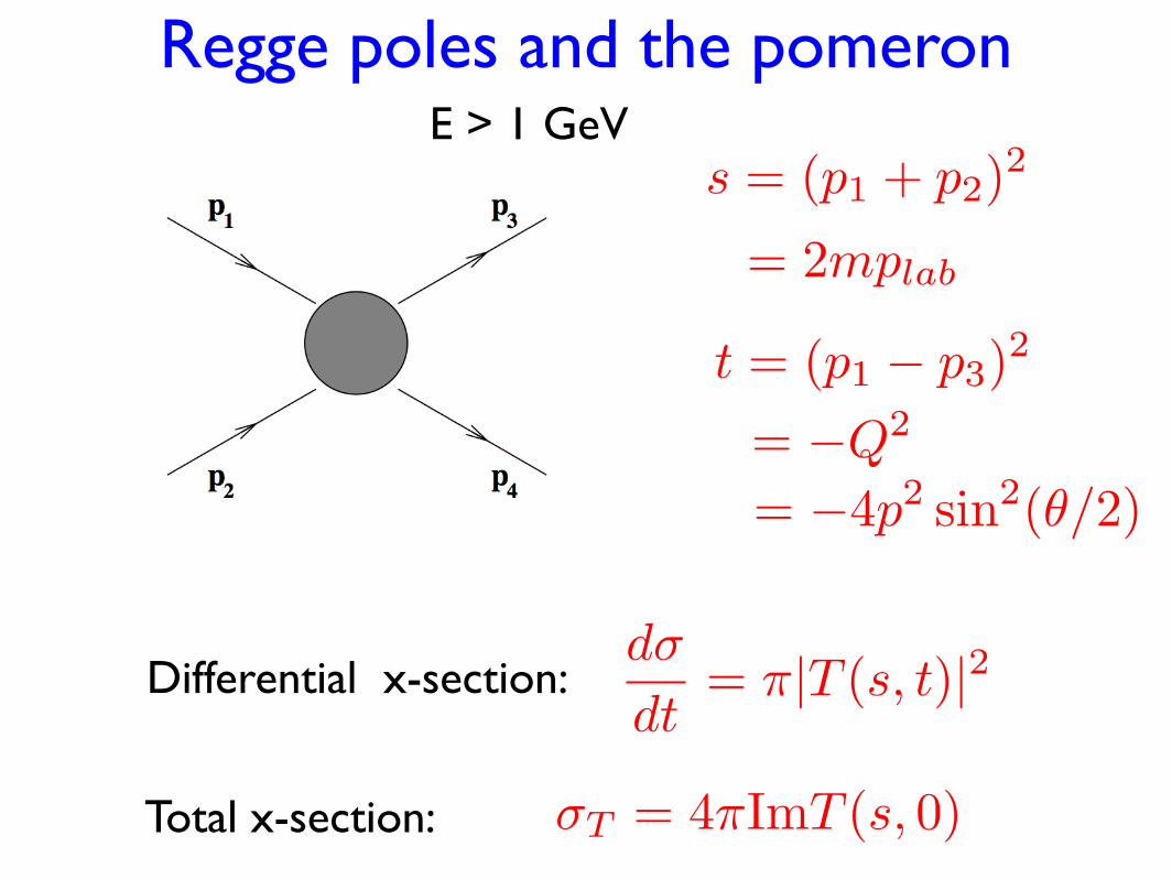
Regge poles and the pomeron

d!

dt= "|T (s, t)|2

s = (p1 + p2)2

t = (p1 ! p3)2

= 2mplab

= !Q2

= !4p2 sin2(!/2)

Differential x-section:

Total x-section: !T = 4"ImT (s, 0)

E > 1 GeV

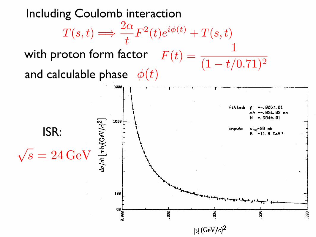
Including Coulomb interaction

with proton form factor

T (s, t) =!2!

tF 2(t)ei!(t) + T (s, t)

F (t) =1

(1 ! t/0.71)2and calculable phase !(t)

ISR:!

s = 24 GeV

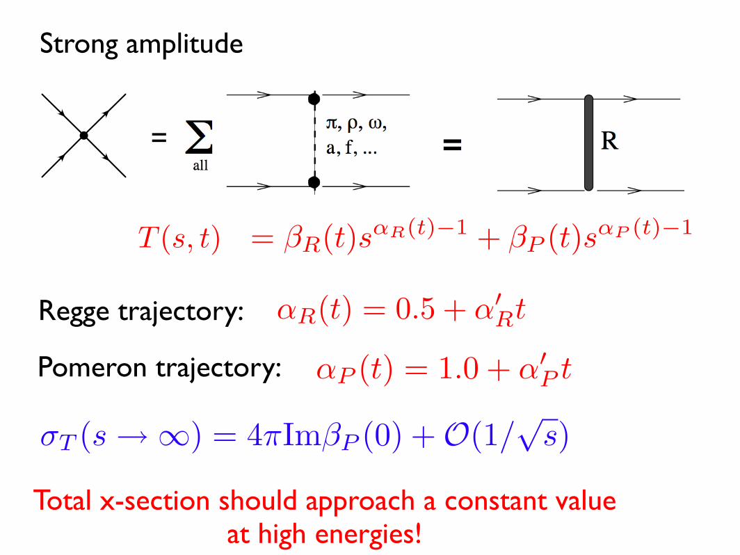
Strong amplitude

= !R(t)s!R(t)!1 + !P (t)s!P (t)!1

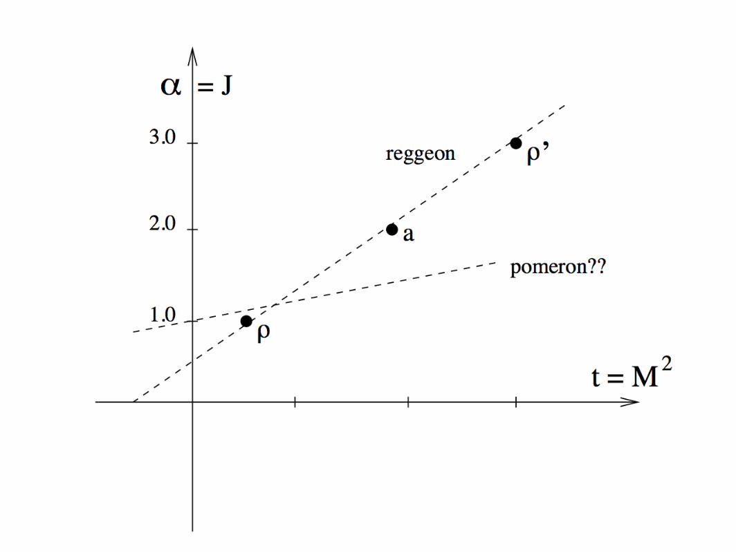
Regge trajectory:

Pomeron trajectory: !P (t) = 1.0 + !!

P t

Total x-section should approach a constant value at high energies!

!T (s ! ") = 4"Im#P (0) + O(1/#

s)

!R(t) = 0.5 + !!

Rt


Veff = C!(r)


a in first Born

approximation.


L = i"!" +1

2M"!

!2" ! C

2("!")2


G0(E,p) =1

E ! p2/2M + i#



4

T (s, t)

=

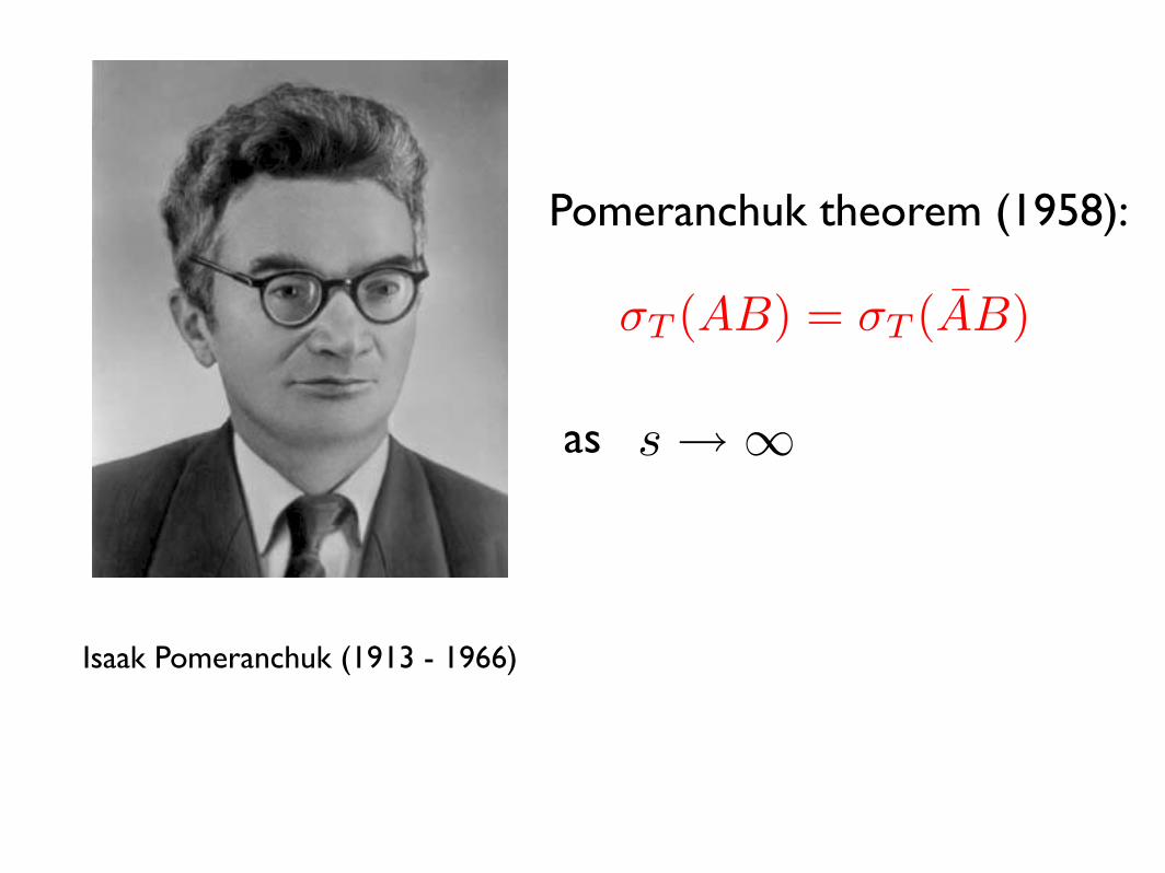
Isaak Pomeranchuk (1913 - 1966)

Pomeranchuk theorem (1958):

s ! "as

!T (AB) = !T (AB)

expansion:

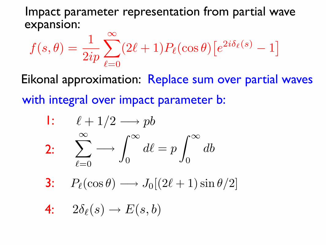
f(s, !) =1

2ip

!!

!=0

(2" + 1)P!(cos !)"

e2i"!(s)! 1

#

Eikonal approximation: Replace sum over partial waves

with integral over impact parameter b:

! + 1/2 !" pb1:

2:!!

!=0

!"

"!

0

d! = p

"!

0

db

3: P!(cos !) !" J0[(2" + 1) sin !/2]

4: 2!!(s) ! E(s, b)

Impact parameter representation from partial wave

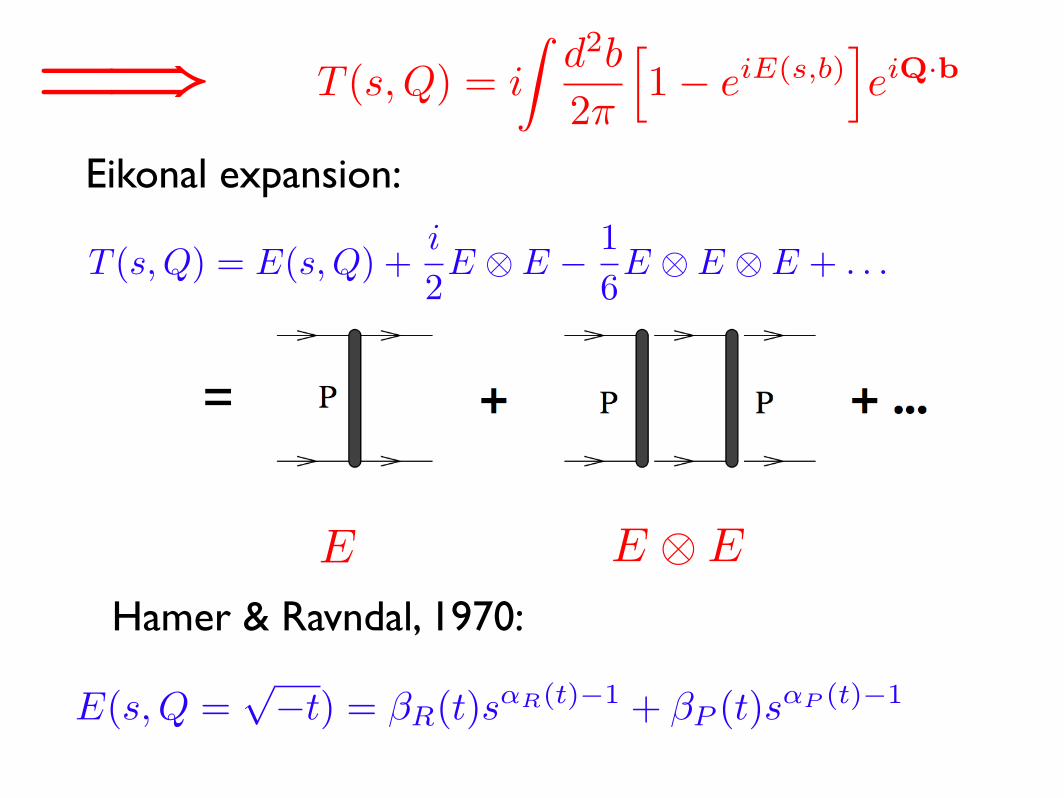
Eikonal expansion:

T (s, Q) = E(s, Q) +i

2E ! E "

1

6E ! E ! E + . . .

E ! EE

E(s, Q =!

"t) = !R(t)s!R(t)!1 + !P (t)s!P (t)!1

Hamer & Ravndal, 1970:

=

T (s, Q) = i

!

d2b

2!

"

1 ! eiE(s,b)#

eiQ·b=!

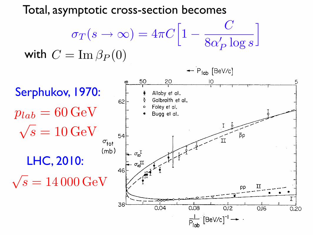
Total, asymptotic cross-section becomes

!T (s ! ") = 4"C

!

1 #

C

8#!

Plog s

"

with C = Im !P (0)

Serphukov, 1970:

LHC, 2010:

plab = 60 GeV!

s = 10 GeV

!

s = 14 000 GeV

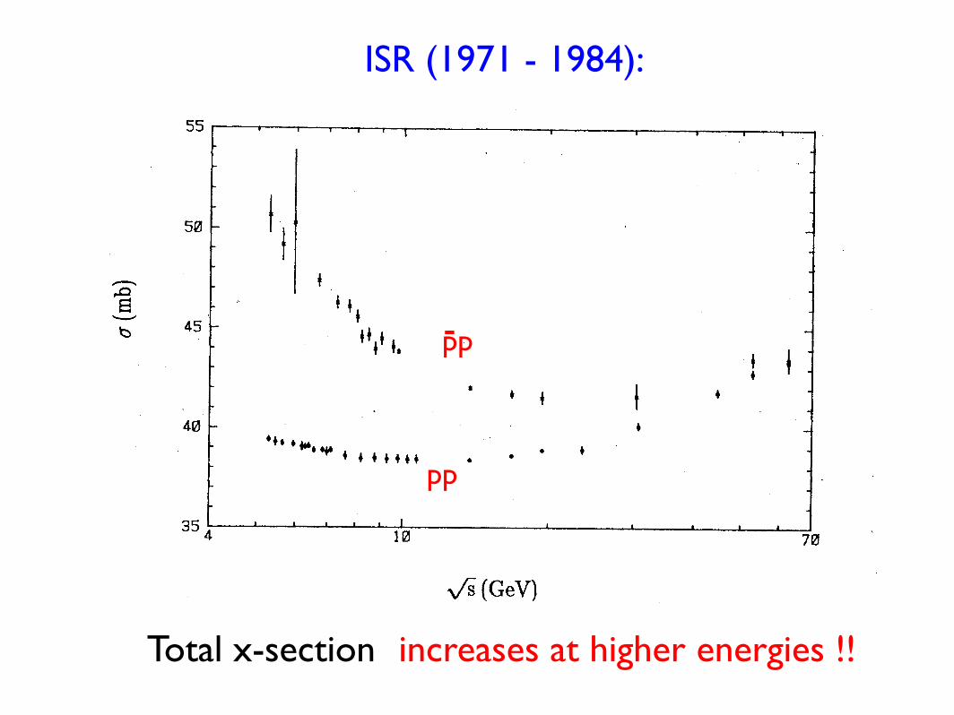
ISR (1971 - 1984):

pp

-pp

Total x-section increases at higher energies !!

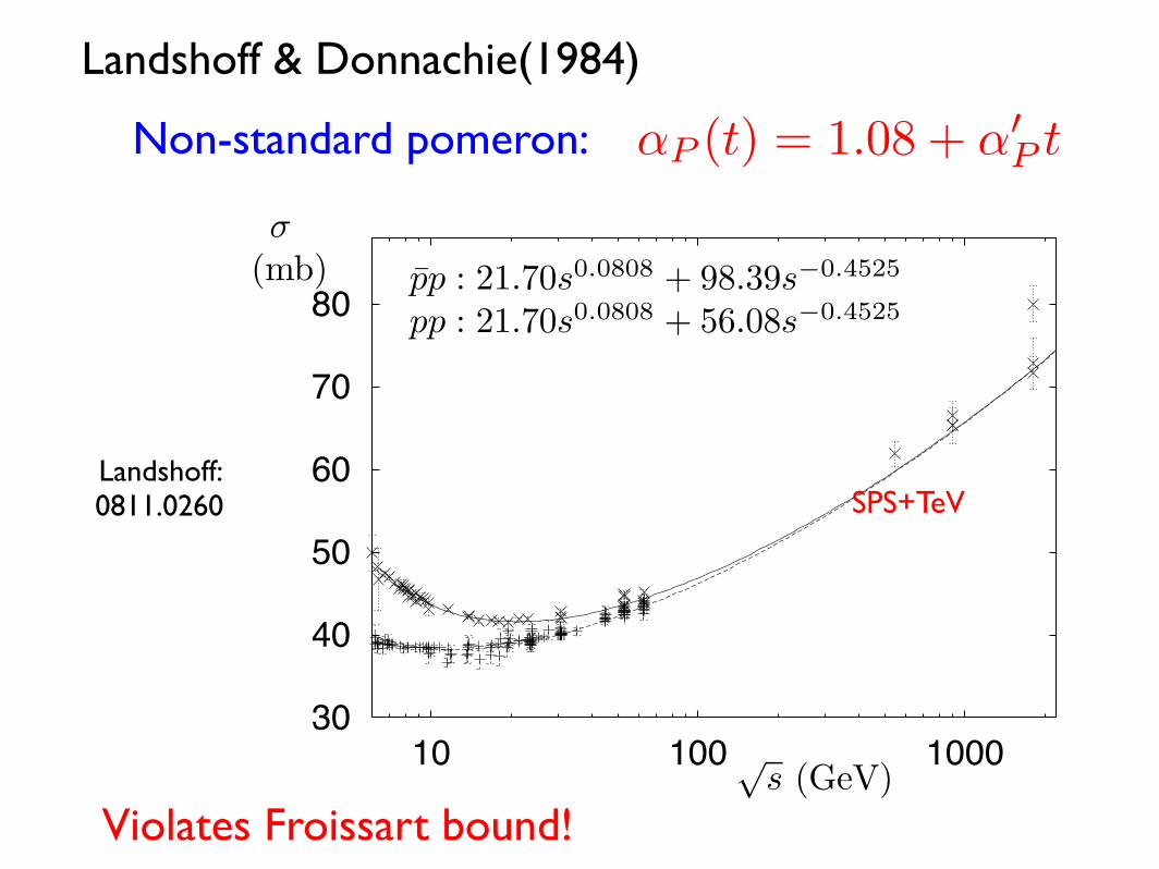
Landshoff & Donnachie(1984)

Non-standard pomeron:

arX

iv:0

811.0

260v1 [h

ep-p

h]

3 N

ov 2

008

How well can we predict the total cross section atthe LHC?

P V Landshoff

Department of Applied Mathematics and Theoretical PhysicsUniversity of CambridgeCambridge CB3 0WA

England

Abstract. Independently of any theory, the possibility that the large value of the Tevatron crosssection claimed by CDF is correct suggests that the total cross section at the LHC may be large.Because of the experimental and theoretical uncertainities, the best prediction is 125±35 mb.

PACS: 13.85.Lg 13.85.Dz 13.60.Hb 11.55.Jy

This talk is based on work with Polkinghorne, Donnachie, Nachtmann and others

going back to 1970. Further details may be found in our book[1].While theoreticalunderstanding of long-range strong interactions has increased greatly since then, it is

still not good enough to allow a confident prediction of even the value of the total cross

section at the LHC. When I prepared this talk, I quoted 125±25 mb, but at the meeting

Alan Martin predicted 90 mb.

Alan Martin’s prediction is viable only if one believes that the CDF measurement[2]

of the pp cross section at the Tevatron is wrong. This is the upper of the!s = 1800

Gev data points shown in figure 1. The curves in the figure are based on !,", f2,a2 and

soft-pomeron exchange, and they go nicely through the E710 Tevatron data point[3]. At!s = 14 TeV only the soft-pomeron term 21.7s0.0808 survives, giving a prediction of

101.5 mb.

30

40

50

60

70

80

10 100 1000

pp : 21.70s0.0808 + 98.39s!0.4525

pp : 21.70s0.0808 + 56.08s!0.4525

!(mb)

!s (GeV)

Figure 1: pp and pp total cross sections

A significant discovery at HERA was that soft-pomeron exchange does not describe

the rise at small x of the proton structure function F2(x,Q2). That is, a term that behaves

SPS+TeV

Violates Froissart bound!

!P (t) = 1.08 + !!

P t

Landshoff: 0811.0260

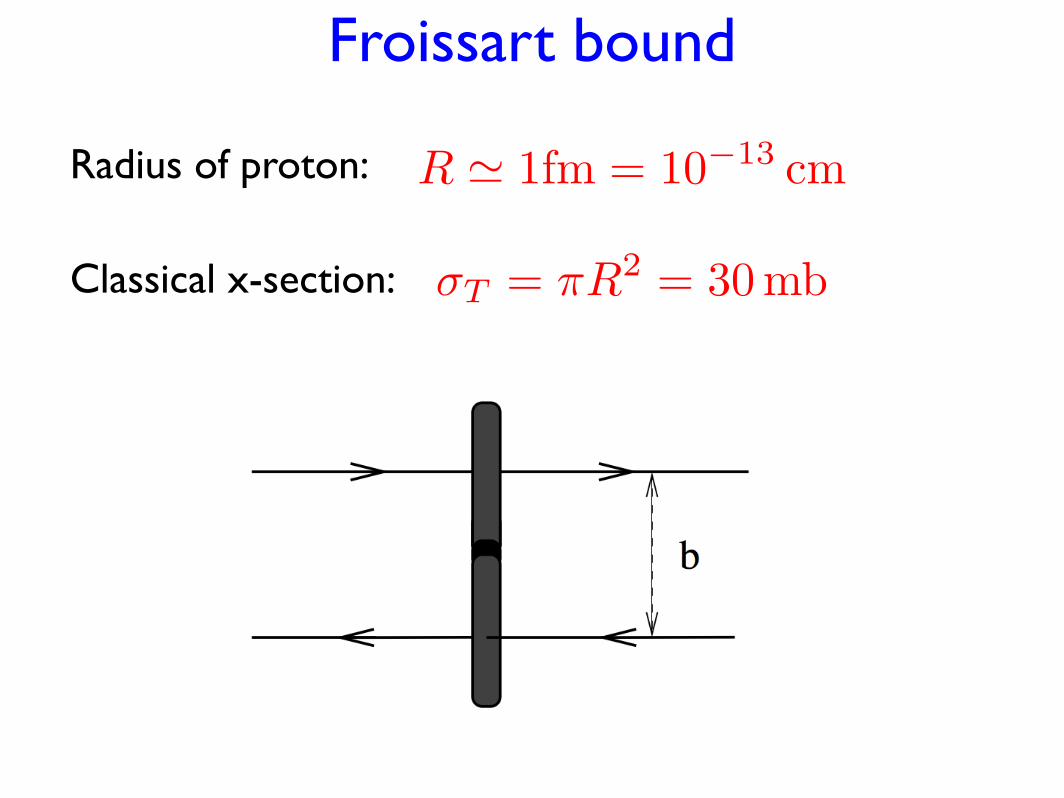
Froissart bound

Radius of proton: R ! 1fm = 10!13

cm

Classical x-section: !T = "R2

= 30 mb

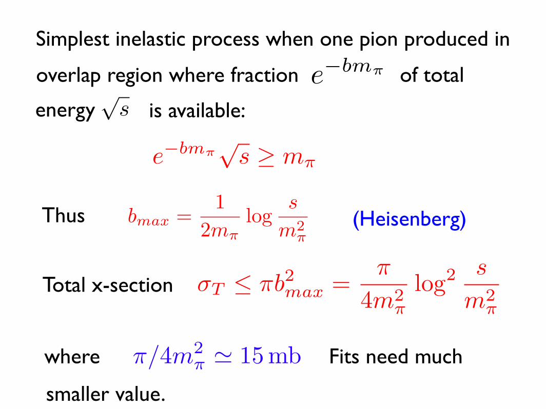
Simplest inelastic process when one pion produced in

overlap region where fraction e!bm! of total

energy !

s is available:

e!bm!

!s " m!

Thus bmax =1

2m!

logs

m2!

(Heisenberg)

Total x-section !T ! "b2

max ="

4m2!

log2 s

m2!

!/4m2

!! 15 mbwhere Fits need much

smaller value.

3

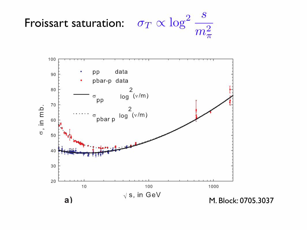
FIG. 2: The saturated Froissart bound fit[13] of total crosssection !pp, " vs.

!s, in GeV, for pp (squares) and pp (circles)

accelerator data: (a) !pp, in mb, (b) "; (c) the nuclear slopeB, in GeV!2 vs.

!s, in GeV, from a QCD-inspired fit[16].

intersections of the B-!pp curve with the !prodp!air curves in

Fig. 1. Figure 3 furnishes cosmic ray experimenters withan easy method to convert their measured !prod

p!air to !pp,

and vice versa. The percentage error in !prodp!air is ! 0.4%

near !prodp!air = 450mb, due to the error in !pp from model

parameter uncertainties.

FIG. 3: A plot of the predicted total pp cross section !pp, inmb vs. the measured p-air cross section, !prod

p!air, in mb.

Determining the k value. It is important at this pointto recall Eq. (1), !m = k"p!air, thus rewinding us ofthe fact that in Method I, the extraction of "p!air (or

!prodp!air) from the measurement of !m requires knowing

the parameter k. The measured depth Xmax at whicha shower reaches maximum development in the atmo-sphere, which is the basis of the cross section measure-ment in Ref. [1], is a combined measure of the depth of

the first interaction, which is determined by the inelasticcross section, and of the subsequent shower development,which has to be corrected for. The model dependent rateof shower development and its fluctuations are the originof the deviation of k from unity in Eq. (1). As seen in Ta-ble I, its values range from 1.6 for a very old model wherethe inclusive cross section exhibited Feynman scaling, to1.15 for modern models with large scaling violations.

Adopting the same strategy that earlier had been usedby Block et al.[17], we decided to match the data to ourprediction of !prod

p!air(s) in order to extract a common valuefor k. This neglects the possibility of a weak energy de-pendence of k over the range measured, found to be verysmall in the simulations of Ref. [9]. By combining theresults of Fig. 2 (a) and Fig. 3, we obtain our predictionof !prod

p!air vs."

s, which is shown in Fig. 4. To deter-

mine k, we leave it as a free parameter and make a #2 fitto rescaled !prod

p!air(s) values of Fly’s Eye, [1]AGASSA[2],EAS-TOP[4] and Yakutsk[3], which are the experimentsthat need a common k-value.

Figure 4 is a plot of !prodp!air vs.

"s, the cms energy

in GeV, for the two di"erent types of experimental ex-traction, using Methods I and II described earlier. Plot-ted as published is the HiRes value at

"s = 77 TeV,

since it is an absolute measurement. We have rescaledin Fig. 4 the published values of !prod

p!air for Fly’s Eye[1],AGASSA[2], Yakutsk[3] and EAS-TOP[4], against ourprediction of !prod

p!air, using the common value of k =

1.264 ± 0.033 ± 0.013 obtained from a #2 fit, and it isthe rescaled values that are plotted in Fig. 4. The er-ror in k of 0.033 is the statistical error of the #2 fit,whereas the error of 0.013 is the systematic error due tothe error in the prediction of !prod

p!air. Clearly, we have

FIG. 4: A #2 fit of the renormalized AGASA, EASTOP, Fly’sEye and Yakutsk data for !prod

p!air, in mb, as a function of theenergy,

!s, in GeV. The result of the fit for the parameter

k in Eq. (1) is k = 1.263 ± 0.033. The HiRes point (soliddiamond), at

!s = 77 GeV, is the model-independent HiRes

experiment, which has not been renormalized.

Froissart saturation: !T ! log2 s

m2!

M. Block: 0705.3037

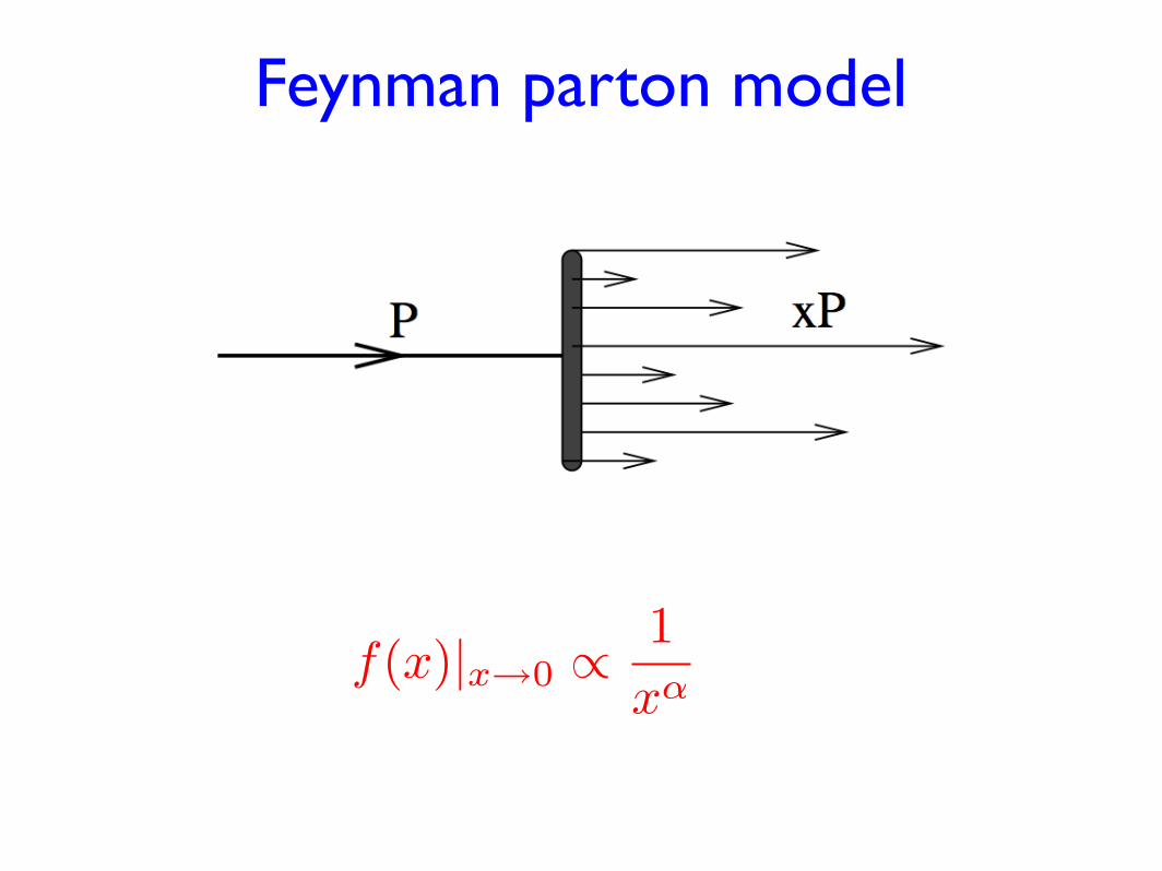
Feynman parton model

f(x)|x!0 !1

x!

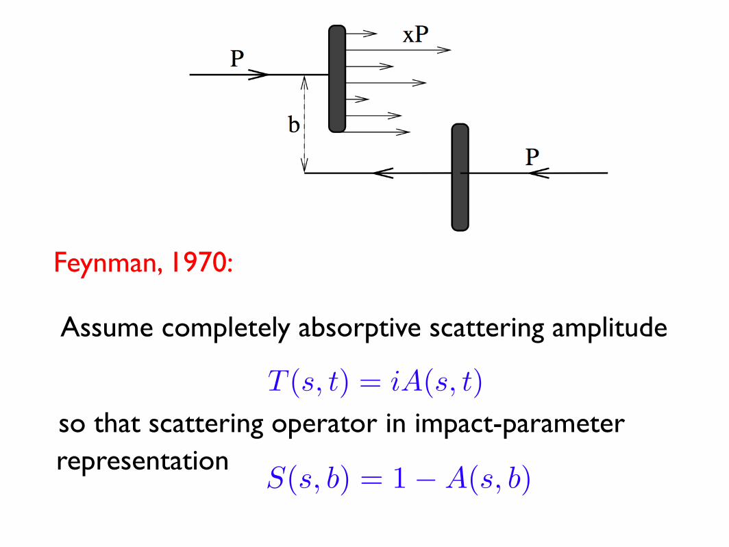
Feynman, 1970:

Assume completely absorptive scattering amplitude

T (s, t) = iA(s, t)

so that scattering operator in impact-parameter

S(s, b) = 1 ! A(s, b)representation

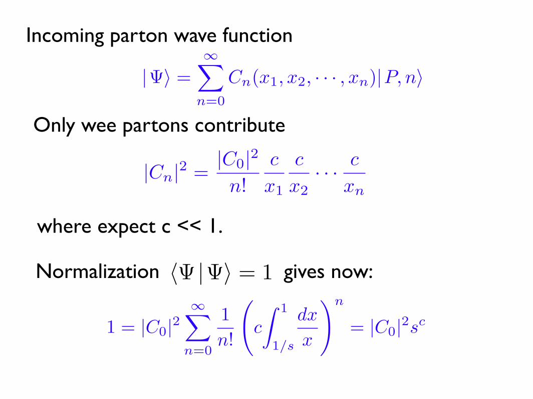
Incoming parton wave function

|!! =!!

n=0

Cn(x1, x2, · · · , xn)|P, n!

Only wee partons contribute

|Cn|2

=|C0|2

n!

c

x1

c

x2

· · ·c

xn

where expect c << 1.

Normalization !! |!" = 1 gives now:

1 = |C0|2

!!

n=0

1

n!

"

c

# 1

1/s

dx

x

$n

= |C0|2s

c

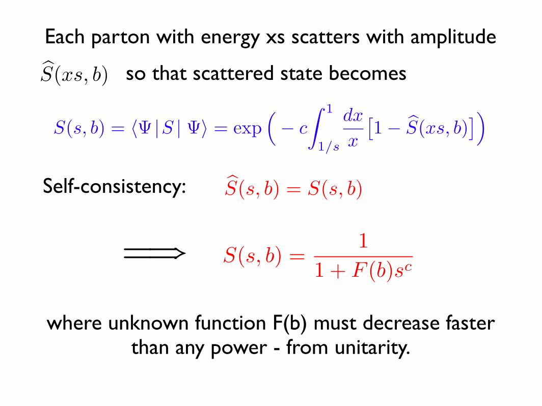
Each parton with energy xs scatters with amplitude

!S(xs, b) so that scattered state becomes

S(s, b) = !! |S | !" = exp!# c

" 1

1/s

dx

x

#1 # $S(xs, b)

%&

Self-consistency: !S(s, b) = S(s, b)

=! S(s, b) =1

1 + F (b)sc

where unknown function F(b) must decrease faster than any power - from unitarity.

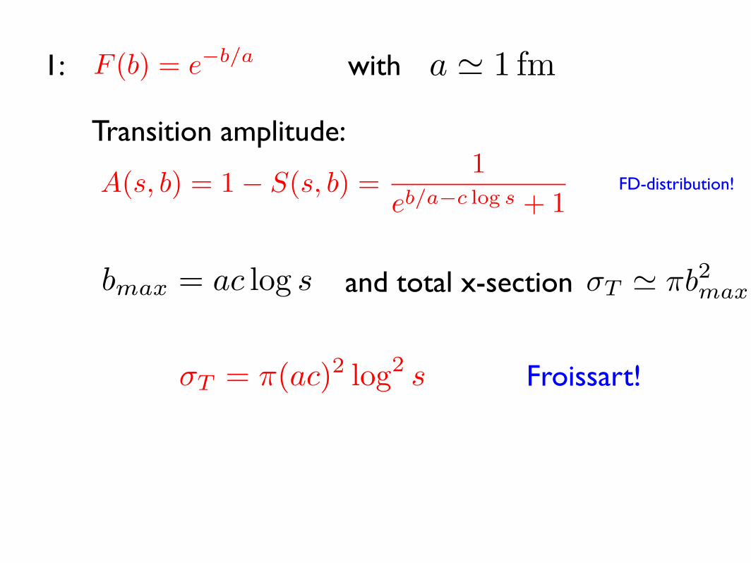
1: F (b) = e!b/a

a ! 1 fmwith

Transition amplitude:

A(s, b) = 1 ! S(s, b) =1

eb/a!c log s + 1FD-distribution!

bmax = ac log s and total x-section !T ! "b2

max

!T = "(ac)2 log2s Froissart!

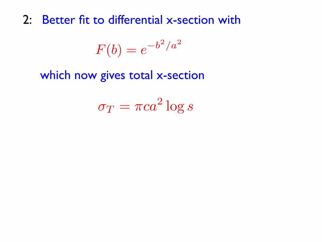
2: Better fit to differential x-section with

F (b) = e!b2/a2

which now gives total x-section

!T = "ca2 log s

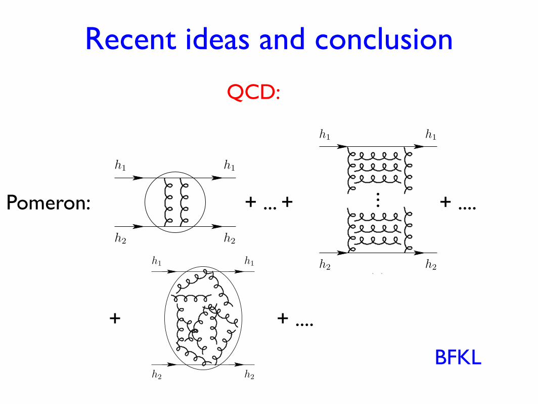
Recent ideas and conclusion

QCD:

BFKL

?

(a)h2 h2

(b)h2 h2

h1 h1h1h1

h1 h1

h2 h2

(e)

h1 h1

(d)h2 h2

(c)h2 h2

h1 h1

Figure 3: Hadron-hadron scattering: (a) what happens?, (b) phenomenological pomeron and(c) two gluon exchange, (d) exchange of a reggeised gluon ladder and (e) in the fluctuatingvacuum gluon field

pomeron is a single Regge pole, consists of two Regge poles, is maybe a Regge cut, and so on.Nevertheless, the assumption that the pomeron seen in elastic hadron-hadron scattering is asimple Regge pole works extremely well phenomenologically.

We discuss as an example the Donnachie-Landsho! (DL) Ansatz [4] for the soft pomeronin Regge theory. The DL pomeron is assumed to be e!ectively a simple Regge pole. Consideras an example p ! p elastic scattering

p(p1) + p(p2) " p(p3) + p(p4), (2.1)

s = (p1 + p2)2, t = (p1 ! p3)

2, (2.2)

where s and t are the c.m. energy squared and the momentum transfer squared. The corre-sponding diagram is as in figure 3b, setting h1 = h2 = p. In the DL Ansatz the wavy line infigure 3b can be interpreted as an e!ective pomeron propagator given by

(!is!!

P)!P(t)"1. (2.3)

Here !P(t) is the pomeron trajectory which is assumed to be linear in t.

!P(t) = !P(0) + !!

Pt (2.4)

3

?

(a)h2 h2

(b)h2 h2

h1 h1h1h1

h1 h1

h2 h2

(e)

h1 h1

(d)h2 h2

(c)h2 h2

h1 h1




p(p1) + p(p2) " p(p3) + p(p4), (2.1)

s = (p1 + p2)2, t = (p1 ! p3)

2, (2.2)


(!is!!

P)!P(t)"1. (2.3)


!P(t) = !P(0) + !!

Pt (2.4)

3

?

(a)h2 h2

(b)h2 h2

h1 h1h1h1

h1 h1

h2 h2

(e)

h1 h1

(d)h2 h2

(c)h2 h2

h1 h1




p(p1) + p(p2) " p(p3) + p(p4), (2.1)

s = (p1 + p2)2, t = (p1 ! p3)

2, (2.2)


(!is!!

P)!P(t)"1. (2.3)


!P(t) = !P(0) + !!

Pt (2.4)

3

+ ... + + ....

+ + ....

Pomeron:

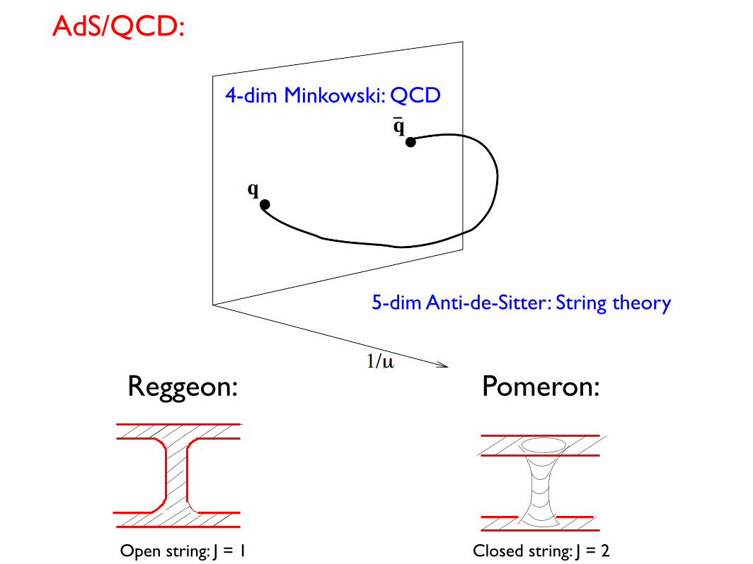
AdS/QCD:4 proceedings printed on April 22, 2008

a strongly coupled plasma of deconfined gauge fields. In this case, onemay expect that features of the AdS/CFT correspondence may be rele-vant. Hence this problem appears to give a stimulating testing ground forthe Gauge/Gravity correspondence and its physical relevance for QCD andparticle physics.

Our aim in these lectures is to provide one possible introduction tothose aspects of the construction of string theory and its applications,mainly the AdS/CFT correspondence, which could be of interest for the stu-dents in QCD and QGP phenomenology. The presentation is thus “strong-interaction oriented”, with both reasons that it uses as much as possible theparticle language, and that the speaker is more appropriately considered asa particle physicist than a string theorist. In this respect he is deeply grate-ful to his string theorists friends and collaborators, in first place RomualdJanik, for their help in many subtle and often technical aspects of stringtheory. In this respect, it is quite stimulating to take part in casting a newbridge between “particles and strings”.

2. The Veneziano Formula and Dual Resonance Models

Shapiro-Virasoro AmplitudeVeneziano Amplitude

{q^2

A (s,q^2) A (s,q^2)R P

s{

Fig. 1. “Duality Diagrams” representing the Veneziano and Shapiro-Virasoro am-plitudes. The hatched surface gives a representation of the string worldsheet of theprocess. s (resp. q2) are the square of the c.o.m. energy (resp. momentum trans-fer) of the 2-body scattering amplitude. AR(s, q2) is, at high energy, the Reggeonamplitude; AP (s, q2) is the Pomeron amplitude, see text.

The Veneziano amplitude was the e!ective starting point of string the-ory, even if it took some years to fully realize the connection. At first theVeneziano amplitude was proposed as a way to formulate mathematically

Reggeon:

4 proceedings printed on April 22, 2008

a strongly coupled plasma of deconfined gauge fields. In this case, onemay expect that features of the AdS/CFT correspondence may be rele-vant. Hence this problem appears to give a stimulating testing ground forthe Gauge/Gravity correspondence and its physical relevance for QCD andparticle physics.

Our aim in these lectures is to provide one possible introduction tothose aspects of the construction of string theory and its applications,mainly the AdS/CFT correspondence, which could be of interest for the stu-dents in QCD and QGP phenomenology. The presentation is thus “strong-interaction oriented”, with both reasons that it uses as much as possible theparticle language, and that the speaker is more appropriately considered asa particle physicist than a string theorist. In this respect he is deeply grate-ful to his string theorists friends and collaborators, in first place RomualdJanik, for their help in many subtle and often technical aspects of stringtheory. In this respect, it is quite stimulating to take part in casting a newbridge between “particles and strings”.

2. The Veneziano Formula and Dual Resonance Models

Shapiro-Virasoro AmplitudeVeneziano Amplitude

{q^2

A (s,q^2) A (s,q^2)R P

s{

Fig. 1. “Duality Diagrams” representing the Veneziano and Shapiro-Virasoro am-plitudes. The hatched surface gives a representation of the string worldsheet of theprocess. s (resp. q2) are the square of the c.o.m. energy (resp. momentum trans-fer) of the 2-body scattering amplitude. AR(s, q2) is, at high energy, the Reggeonamplitude; AP (s, q2) is the Pomeron amplitude, see text.

The Veneziano amplitude was the e!ective starting point of string the-ory, even if it took some years to fully realize the connection. At first theVeneziano amplitude was proposed as a way to formulate mathematically

Pomeron:

Open string: J = 1 Closed string: J = 2

4-dim Minkowski: QCD

5-dim Anti-de-Sitter: String theory

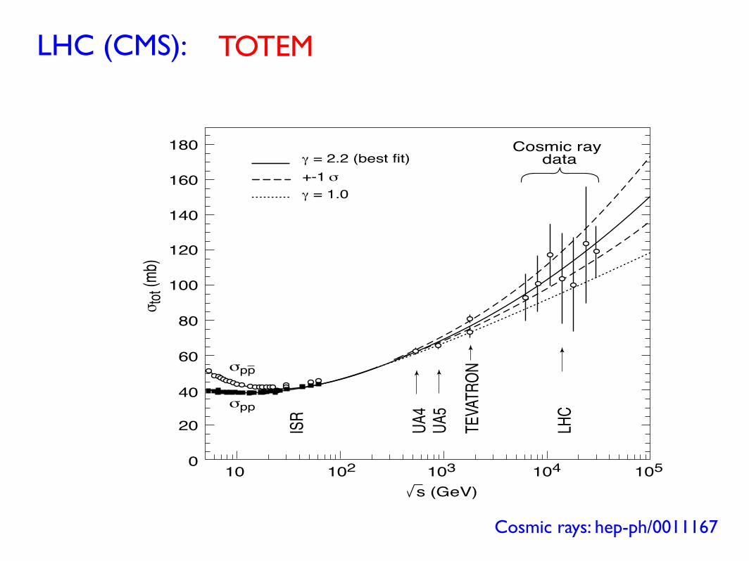
TABLE 1. !pptot data from high

energy accelerators: fits values are

from [5].

!s (TeV) !pp

tot (mb)0.55 Fit 61.8 ± 0.7

UA4 62.2 ± 1.5CDF 61.5 ± 1.0

1.8 Fit 76.5 ± 2.3E710 72.8 ± 3.1CDF 80.6 ± 2.3

14 Fit 109.0 ± 8.030 Fit 126.0± 11.040 Fit 130.0± 13.0

experimental knowledge for both !pptot and !pp

tot are plotted in figure 1. We have alsoplotted the cosmic ray experimental data from AKENO (now AGASSA) [23] andthe Fly’s Eye experiment [24,25]. The curve is the result of the fit described in [5].The increase in !pp

tot as the energy increases is clearly seen. Numerical predictionsfrom this analysis are given in Table 1. It should be remarked that at the LHCenergies and beyond the fitting results display relatively high error values, equal orbigger than 8 mb. We conclude that it is necessary to look for ways to reduce theerrors and make the extrapolations more precise.

0

20

40

60

80

100

120

140

Cosmic ray data

160

180

10 102 103 104 105

s (GeV)

! tot

(mb)

!pp

!pp

" = 2.2 (best fit)

+-1 !

" = 1.0

ISR

TEVA

TRO

N

UA

4U

A5

LHC

FIGURE 1. Experimental !pptot and !pp

tot with the prediction of [5].Cosmic rays: hep-ph/0011167

LHC (CMS): TOTEM

Page 1 of 1

Untitled 3 11/11/2009 15:52

Documents

Proton-proton scattering from low to LHC-energiesfolk.uio.no/finnr/talks/pp-scattering.pdf · Proton-proton scattering from low to LHC-energies • Coulomb scattering • Low-energy