Embed Size (px)
Citation preview

UNIVERSITY OF DELHI BACHELOR OF MATHEMATICS (Hons.)
(BMH)
(Effective from Academic Year 2018-19)
PROGRAMME BROCHURE
XXXXX Revised Syllabus as approved by Academic Council on XXXX, 2018 and
Executive Council on YYYY, 2018

Department of Mathematics, University of Delhi
2
CONTENTS
Page
I. About the Department 3
II. Introduction to CBCS 4
Scope
Definitions
CBCS Course Structure for under-graduate (Hons.) Programme
Semester wise Placement of Courses
III. BMH Programme Details 8
Programme Objectives
Programme Structure
Selection of Elective Courses
Teaching
Teaching Pedagogy
Eligibility for Admissions
Assessment Tasks
Assessment of Students’ Performance
and Scheme of Examination
Pass Percentage & Promotion Criteria:
Semester to Semester Progression
Conversion of Marks into Grades
Grade Points
CGPA Calculation
Division of Degree into Classes
Attendance Requirement
Span Period
Guidelines for the Award of Internal Assessment Marks
BMH Programme (Semester Wise)
IV. Course Wise Content Details for BMH Programme 13

Department of Mathematics, University of Delhi
3
I. About the Department
The impressive tradition of the Department of Mathematics derives its roots from the east
which predates the formation of the post graduate department. Encompassed within the
tradition are names such as P. L. Bhatnagar, J. N. Kapur, A. N. Mitra, and B. R. Seth, all of
whom distinguished themselves by their teaching and research and who later carved out major
roles for themselves on the Indian mathematical scenario even though they were not directly
associated with the post-graduate department.
The Department of Mathematics, University of Delhi took birth in 1947, with Prof. Ram
Behari, as Head of the Department. He can be credited with having started the tradition of
research in Differential Geometry, one of the first disciplines in pure mathematics to have been
pursued in the department. During his tenure in 1957 masters program in Mathematical
Statistics was introduced and the department was renamed as Department of Mathematics and
Mathematical Statistics. In 1962, the department was given a formidable push when a
distinguished mathematician, Prof. R. S. Varma, assumed the responsibilities of the Head. The
first masters program in Operational Research in the country was started in this department
under the leadership of Prof. R. S. Varma. This was even before any university in the U.K.,
and in several other advanced countries had done so. Since the activities and the courses in the
department were now so wide and varied the department was enlarged into the Faculty of
Mathematics at the initiative of Prof. R. S. Varma. In 1970, another distinguished
mathematician, Prof. U. N. Singh, was appointed the Head of the Department and the Dean of
the Faculty of Mathematics. He provided the department with the requisite strength and depth
in the core areas of mathematics. He created strong research in Functional Analysis, Harmonic
Analysis, and in Operator Theory. During his stewardship of the department, several
distinguished mathematicians from all over the globe began to visit the department regularly
and the department can be said to have attained full maturity. He foresaw the need to have
separate departments within the overall set-up of the Faculty of Mathematics and thus were
created, in 1973, the Department of Mathematics, the Department of Statistics, the Department
of Operational Research and the Department of Computer Science. The Faculty of Mathematics
was re-designated as the Faculty of Mathematical Sciences.
The Department of Mathematics offers a Bachelor of Mathematics (Hons.) (BMH) course
through constituent colleges of the University of Delhi besides offering Masters Programme in
Mathematics and two research programmes, M.Phil. and Ph.D. in Mathematics.
We are highly rated in various rankings such as we are ranked 10 in Times Higher Education
Ranking in India and 144 in Asia in 2018. Inputs are taken from various stakeholders including
students, alumni, parents at different stages of the preparation of the syllabus.

Department of Mathematics, University of Delhi
4
II. Introduction to CBCS (Choice Based Credit System)
Choice Based Credit System:
The CBCS provides an opportunity for the students to choose courses from the prescribed
courses comprising core, elective/minor or skill-based courses. The courses can be evaluated
following the grading system, which is considered to be better than the conventional marks
system. Grading system provides uniformity in the evaluation and computation of the
Cumulative Grade Point Average (CGPA) based on student’s performance in examinations
enables the student to move across institutions of higher learning. The uniformity in evaluation
system also enable the potential employers in assessing the performance of the candidates.
Definitions:
(i) ‘Academic Programme’ means an entire course of study comprising its programme
structure, course details, evaluation schemes etc. designed to be taught and evaluated in a
teaching Department/Centre or jointly under more than one such Department/Centre.
(ii) ‘Course’ means a segment of a subject that is part of an Academic Programme.
(iii) ‘Programme Structure’ means a list of courses (Core, Elective, Open Elective) that makes
up an Academic Programme, specifying the syllabus, Credits, hours of teaching, evaluation
and examination schemes, minimum number of credits required for successful completion of
the programme etc. prepared in conformity to University Rules, eligibility criteria for
admission.
(iv) ‘Core Course’ means a course that a student admitted to a particular programme must
successfully complete to receive the degree and which cannot be substituted by any other
course.
(v) ‘Elective Course’ means an optional course to be selected by a student out of such courses
offered in the same or any other Department/Centre.
(vi) ‘Discipline Specific Elective (DSE)’ Course is the domain specific elective course offered
by the main discipline/subject of study. The University/Institute may also offer discipline
related Elective courses of interdisciplinary nature also, but these are needed to be offered by
main discipline/subject of study.
(vii) ‘Dissertation/Project’ is an elective course designed to acquire special/advanced
knowledge, such as supplement study/support study to a project work, and a candidate studies
such a course on his own with an advisory support by a teacher/faculty member. Project
work/Dissertation is considered as a special course involving application of knowledge in
solving /analysing /exploring a real life situation/difficult problem. A Project/Dissertation work
would be of 6 credits. A Project/Dissertation work may be given in lieu of a discipline specific
elective paper.
(viii) ‘Generic Elective (GE)’ Course is an elective course chosen generally from an unrelated
discipline/subject, with an intention to seek exposure to other disciplines. A core course offered

Department of Mathematics, University of Delhi
5
in a discipline/subject may be treated as an elective by other discipline/subject and vice versa
and such electives may also be referred to as Generic Elective.
(ix) ‘Ability Enhancement Courses (AEC)’ also referred as Competency Improvement
Courses/Skill Development Courses/Foundation Course. The Ability Enhancement Courses
(AEC) may be of two kinds: AE Compulsory Course (AECC) and AE Elective Course (AEEC).
(x) ‘AECC’ are the courses based upon the content that leads to Knowledge enhancement. The
two AECC are: Environmental Science, English/MIL Communication.
(xi) ‘AEEC’ are value-based and/or skill-based and are aimed at providing hands-on-training,
competencies, skills, etc. These courses may be chosen from a pool of courses designed to
provide value-based and/or skill-based instruction. These courses are also referred to as Skill
Enhancement Courses (SEC).
(vii) ‘Credit’ means the value assigned to a course which indicates the level of instruction;
One-hour lecture per week equals 1 Credit, 2 Hours practical class per week equals 1 credit.
Credit for a practical could be proposed as part of a course or as a separate practical course
(viii) ‘CGPA’ is cumulative grade points calculated for all courses completed by the students
at any point of time.
(ix) ‘SGPA’ means Semester Grade Point Average calculated for individual semester.
(x) ‘CGPA’ is Cumulative Grade Points Average calculated for all courses completed by the
students at any point of time. CGPA is calculated each year for both the semesters clubbed
together.
(xi) ‘Grand CGPA’ is calculated in the last year of the course by clubbing together of CGPA
of two years, i.e., four semesters. Grand CGPA is being given in Transcript form. To benefit
the student a formula for conversation of Grand CGPA into % age marks is given in the
Transcript.

Department of Mathematics, University of Delhi
6
CBCS Course Structure for undergraduate (Hons.) Programme
Course *Credits
Theory + Practical Theory + Tutorial
=========================================================================
I. Core Course 14X4=56 14X5=70
(14 Papers)
Core Course Practical / Tutorial* 14X2=28 14X1=14
(14 Practicals/Tutorials*)
II. Elective Course
(8 Papers)
A.1. Discipline Specific Elective 4X4=16 4X5=20
(4 Papers)
A.2. Discipline Specific Elective
Practical/ Tutorial* 4X2=8 4X1=4
(4 Papers)
B.1. Generic Elective/ Interdisciplinary 4X4=16 4X5=20
(4 Papers)
B.2. Generic Elective Practical/ Tutorial* 4X2=8 4X1=4
(4 Papers)
Optional Dissertation or project work in place of one Discipline Specific Elective paper (6 credits)
in sixth Semester.
III. Ability Enhancement Courses
1. Ability Enhancement Compulsory Courses (AECC) 2X2=4 2X2=4
(2 Papers of 2 credits each)
Environmental Science
English /MIL Communication
2. Ability Enhancement Elective (Skill Based) 2X4=8 2X4=8
(Minimum 2) (SEC)
(2 Papers of 4 credits each)
_________________ _________________
Total credits: 144 144
Note: The institute should evolve a system/ policy about ECA/ General Interest/ Hobby/ Sports/ NCC/ NSS/ related
courses on its own.
* Wherever there is a practical there will be no tutorial and vice-versa

Department of Mathematics, University of Delhi
7
SEMESTER WISE PLACEMENT OF THE COURSES
Sem-
ester
Core Course(14)
Ability Enhancement
Compulsory Course
(AECC)(2)
Skill
Enhancement
Course
(SEC)(2)
Discipline
Specific
Elective
(DSE)(4)
Generic
Elective
(GE)(4)
I BMH101: Calculus
(including practicals) (English
Communication/MIL)/
Environmental Science
GE-1
BMH102: Algebra
II BMH203: Real Analysis (English
Communication/MIL)/
Environmental Science
GE-2
BMH204: Differential
Equations
(including practicals)
III BMH305: Theory of Real
Functions
SEC-1
LaTeX and
HTML
GE-3
BMH306: Group Theory-I
BMH307: Multivariate
Calculus
(including practicals)
IV BMH408: Partial Differential
Equations
(including practicals)
SEC-2
Computer
Algebra
Systems and
Related
Software
GE-4
BMH409: Riemann Integration
and Series of Functions
BMH410: Ring Theory and
Linear Algebra-I
V
BMH511: Metric Spaces
DSE-1
(including
practicals)
DSE-2
BMH512: Group Theory-II
VI BMH613: Complex Analysis
(including practicals) DSE-3
DSE-4
BMH614: Ring Theory and
Linear Algebra-II

Department of Mathematics, University of Delhi
8
III. BMH Programme Details:
Programme Objectives: Students who choose BMH Programme, develop the ability to
think critically, logically and analytically and hence use mathematical reasoning in everyday
life. Pursuing a degree in mathematics will introduce the students to a number of interesting
and useful ideas in preparations for a number of mathematics careers in education, research,
government sector, business sector and industry.
The programme covers the full range of mathematics, from classical Calculus to modern
Cryptography, Information Theory, and Network Security. The course lays a structured
foundation of Calculus, Real & Complex analysis, Abstract Algebra, Differential equations
(including Mathematical modeling), Number theory, Graph theory, and C++ programming
exclusively for mathematics.
An exceptionally broad range of topics covering Pure & Applied Mathematics: Linear Algebra,
Metric spaces, Statistics, Linear Programming, Numerical Analysis, Mathematical Finance,
Coding theory, Mechanics and Bio-Mathematics cater to varied interests and ambitions. Also
hand on sessions in Computer lab using various Computer Algebra Systems (CAS) softwares
such as Mathematica, MATLAB, Maxima, R to have a deep conceptual understanding of the
above tools are carried out to widen the horizon of students’ self-experience.
To broaden the interest for interconnectedness between formerly separate disciplines one can
choose from the list of Generic electives for example one can opt for economics as one of the
GE papers. Skill enhancement Courses enable the student acquire the skill relevant to the main
subject. Choices from Discipline Specific Electives provides the student with liberty of
exploring his interests within the main subject.
Of key importance is the theme of integrating mathematical and professional skills. The well-
structured programme empowers the student with the skills and knowledge leading to enhanced
career opportunities in industry, commerce, education, finance and research.
Programme Learning Outcomes: The completion of the BMH Programme will enable
a student to:
i) Communicate mathematics effectively by written, computational and graphic means.
ii) Create mathematical ideas from basic axioms.
iii) Gauge the hypothesis, theories, techniques and proofs provisionally.
iv) Utilize mathematics to solve theoretical and applied problems by critical understanding,
analysis and synthesis.
v) Identify applications of mathematics in other disciplines and in the real-world, leading
to enhancement of career prospects in a plethora of fields and research.
Programme Structure: The BMH programme is a three-year, six-semesters course. A
student is required to complete 144 credits for completion of the course and award of degree.
Semester Semester
Part – I First Year Semester I: 20 Semester II: 20
Part – II Second Year Semester III: 28 Semester IV: 28
Part - III Third Year Semester V: 24 Semester VI: 24

Department of Mathematics, University of Delhi
9
Semester wise Details of BMH Course & Credit Scheme
Sem-
ester
Core Course(14)
Ability Enhancement
Compulsory Course
(AECC)(2)
Skill
Enhancement
Course
(SEC)(2)
Discipline
Specific
Elective
(DSE)(4)
Generic
Elective
(GE)(4)
Total
Credits
I
L+T/P
BMH101: Calculus
(including practicals) (English
Communication/MIL)/
Environmental
Science
2
GE-1
5+1 = 6
20
BMH102: Algebra
4 + 2 = 6
5 + 1 = 6
II
L+T/P
BMH203: Real
Analysis
(English
Communication/MIL)/
Environmental
Science
2
GE-2
5+1 = 6
20
BMH204: Differential
Equations
(including practicals)
5 + 1 = 6
4 + 2 = 6
III
L+T/P
BMH305: Theory of
Real Functions
SEC-1
LaTeX and
HTML
4
GE-3
5 +1 = 6
28
BMH306: Group
Theory-I
BMH307:
Multivariate Calculus
(including practicals)
5 + 1 = 6, 5 + 1 = 6
4 + 2 = 6
IV
L+T/P
BMH408: Partial
Differential Equations
(including practicals)
SEC-2
Computer
Algebra
Systems and
Related
Software
4
GE-4
5 +1 = 6
28
BMH409: Riemann
Integration and Series
of Functions
BMH410: Ring
Theory and Linear
Algebra-I
4 + 2 = 6, 5 + 1 = 6
5 + 1 = 6
V
L+T/P
BMH511: Metric
Spaces
DSE-1
(including
practicals)
DSE-2
4 + 2 = 6
5 + 1 = 6
24
BMH512: Group
Theory-II
5 + 1 = 6
5 + 1 = 6

Department of Mathematics, University of Delhi
10
Sem-
ester
Core Course(14)
Ability Enhancement
Compulsory Course
(AECC)(2)
Skill
Enhancement
Course
(SEC)(2)
Discipline
Specific
Elective
(DSE)(4)
Generic
Elective
(GE)(4)
Total
Credits
VI
L+T/P
BMH613: Complex
Analysis
(including practicals)
DSE-3
DSE-4
5 + 1 = 6
5 + 1 = 6
24
BMH614: Ring
Theory and Linear
Algebra-II
4 + 2 = 6, 5 + 1 = 6
Total Credits = 144
Legend: L: Lecture Class; T: Tutorial Class; P: Practical Class
Note: One-hour lecture per week equals 1 Credit, 2 Hours practical class per week equals 1 credit.
Practical in a group of 15-20 students in Computer Lab and Tutorial in a group of 8-12 students.
List of Discipline Specific Elective (DSE) Courses:
DSE-1 (including practicals): Any one of the following
(at least two shall be offered by the college)
(i). Numerical Analysis
(ii). Mathematical Modeling and Graph Theory
(iii). C++ Programming for Mathematics
DSE-2: Any one of the following (at least two shall be offered by the college)
(i). Probability Theory and Statistics
(ii). Discrete Mathematics
(iii). Cryptography and Network Security
DSE-3: Any one of the following (at least two shall be offered by the college)
(i). Mathematical Finance
(ii). Introduction to Information Theory and Coding
(iii). Biomathematics
DSE-4: Any one of the following (at least two shall be offered by the college)
(i). Number Theory
(ii). Linear Programming and Applications
(iii). Mechanics

Department of Mathematics, University of Delhi
11
Teaching:
The faculty of the Department is primarily responsible for organizing lecture work for
BMH. The instructions related to tutorials are provided by the respective registering units
under the overall guidance of the Department. Faculty from some other Departments and
constituent colleges are also associated with lecture and tutorial work in the Department.
There shall be 90 instructional days excluding examination in a semester.
(Add details about Projects/Dissertation and role of supervisor)
Teaching Pedagogy:
Teaching pedagogy involving class room interactions, discussion, presentation etc. to be
detailed out. The description should not be more than 300 words and could be both in
general for all the courses and even for some particular papers requiring specific pedagogy
like project work, group activities, or live projects.
This section (for each paper) could include the class-wise/week-wise flow of the course.
Eligibility for Admissions:
Senior Secondary School Certificate Examination (Class XII) of the Central Board of
Secondary Education or an examination recognized as equivalent thereto.
50% marks in Mathematics and an aggregate of 45% marks in the qualifying examination.
(Relaxation will be given to the candidates belongin SC, ST and OBC category as per the
University rules).
Specific Requirements: The merit shall be determined on the basis of aggregate of marks
obtained in Mathematics, one language paper and two best elective subjects under academic
stream.
Assessment Tasks:
Comprising MCQs, Project work and presentations, design and production of course related
objects, written assignments, open or closed book exams specifically designed to assess the
Learning Outcomes. (Evidence of achieving the Outcomes).
Assessment of Students’ Performance and Scheme of Examinations:
i ) English shall be the medium of instruction and examination. i i ) Assessment of students’ performance shall consist of:
(Point wise details of internal assessment and end semester examination, their
weightage and scheme to be given)
It is mentioned along with course content of respective courses.
Pass Percentage & Promotion Criteria: As per University Examination rule.
Part to Part Progression: As per University Examination rule
Department of Mathematics, University of Delhi
12
Conversion of Marks into Grades: As per University Examination rule
Grade Points: Grade point table as per University Examination rule
CGPA Calculation: As per University Examination rule.
SGPA Calculation: As per University Examination rule
Grand SGPA Calculation: As per University Examination rule
Conversion of Grand CGPA into Marks
As per University Examination rule
Division of Degree into Classes:
As per University Examination rule
Attendance Requirement:
As per University Examination rule
Span Period:
No student shall be admitted as a candidate for the examination for any of the Parts/Semesters
after the lapse of five years from the date of admission to the Part-I/Semester-I of the BMH
Programme.
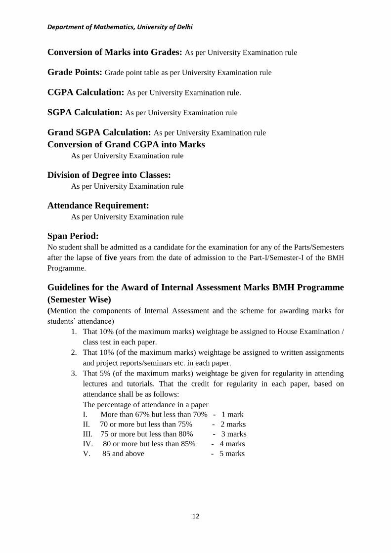
Guidelines for the Award of Internal Assessment Marks BMH Programme
(Semester Wise)
(Mention the components of Internal Assessment and the scheme for awarding marks for
students’ attendance)
1. That 10% (of the maximum marks) weightage be assigned to House Examination /
class test in each paper.
2. That 10% (of the maximum marks) weightage be assigned to written assignments
and project reports/seminars etc. in each paper.
3. That 5% (of the maximum marks) weightage be given for regularity in attending
lectures and tutorials. That the credit for regularity in each paper, based on
attendance shall be as follows:
The percentage of attendance in a paper
I. More than 67% but less than 70% - 1 mark
II. 70 or more but less than 75% - 2 marks
III. 75 or more but less than 80% - 3 marks
IV. 80 or more but less than 85% - 4 marks
V. 85 and above - 5 marks

Department of Mathematics, University of Delhi
13
IV: Course Wise Content Details for BMH Programme:
Bachelor of Mathematics (Hons.)
(BMH)
Semester I
BMH101: Calculus
Total Marks: 150 (Theory: 75, Internal Assessment: 25 and Practical: 50)
Workload: 4 Lectures (per week), 4 Practicals (per week per student)
Duration: 14 Weeks (56 Hrs. Theory + 56 Hrs. Practical) Examination: 3 Hrs.
Course Objectives: The primary objective of this course is to introduce the basic tools of
calculus and geometric properties of different conic sections which are helpful in understanding
their applications in planetary motion, design of telescope and to the real-world problems. Also,
to carry out the hand on sessions in computer lab to have a deep conceptual understanding of
the above tools to widen the horizon of students’ self-experience.
Course Learning Outcomes: This course will enable the students to:
i) Sketch curves in a plane using its mathematical properties in the different coordinate
systems of reference.
ii) Apply derivatives in Optimization, Social sciences, Physics and Life sciences etc.
iii) Compute area of surfaces of revolution and the volume of solids by integrating over
cross-sectional areas.
Course Contents:
Unit 1: Derivatives for Graphing and Applications (Lectures: 12)
The first-derivative test for relative extrema, Concavity and inflection points, Second-
derivative test for relative extrema, Curve sketching using first and second derivative tests;
Limits to infinity and infinite limits, Graphs with asymptotes, L’Hôpital’s rule; Applications
in Business, Economics and Life Sciences; Higher order derivatives, Leibniz rule.
Unit 2: Sketching and Tracing of Curves (Lectures: 16)
Parametric representation of curves and tracing of parametric curves (except lines in 3 ), Polar
coordinates and tracing of curves in polar coordinates; Techniques of sketching conics,
Reflection properties of conics, Rotation of axes and second degree equations, Classification
into conics using the discriminant.
Unit 3: Volume and Area of Surfaces (Lectures: 16)
Volumes by slicing disks and method of washers, Volumes by cylindrical shells, Arc length,
Arc length of parametric curves, Area of surface of revolution; Hyperbolic functions;
Reduction formulae.

Department of Mathematics, University of Delhi
14
Unit 4: Vector Calculus and its Applications (Lectures: 12)
Introduction to vector functions and their graphs, Operations with vector functions, Limits and
continuity of vector functions, Differentiation and integration of vector functions; Modeling
ballistics and planetary motion, Kepler's second law; Unit tangent, Normal and binormal
vectors, Curvature.
References:
1. Anton, Howard, Bivens, Irl, & Davis, Stephen (2013). Calculus (10th ed.). John Wiley
& Sons Singapore Pte. Ltd. Indian Reprint (2016) by Wiley India Pvt. Ltd. Delhi.
2. Osborne, George. A. (1906). Differential and Integral Calculus with Examples and
Applications. Revised Edition. D. C. Health & Co. Publishers. Boston, U.S.A.
3. Strauss, Monty J., Bradley, Gerald L., & Smith, Karl J. (2007). Calculus (3rd ed.).
Dorling Kindersley (India) Pvt. Ltd. (Pearson Education). Delhi. Indian Reprint 2011.
Additional Reading:
1. Thomas, Jr. George B., Weir, Maurice D., & Hass, Joel (2014). Thomas’ Calculus (13th
ed.). Pearson Education, Delhi. Indian Reprint 2017.
Practical / Lab work to be performed in Computer Lab.
List of the practicals to be done using Mathematica /MATLAB /Maple /Scilab/Maxima etc.
(i). Plotting the graphs of the following functions: , [ ] (greatest integer function), ax x
1, | |, | |, , ,n nax b ax b c ax b x x n
1, sin 1 , sin 1 , and , , for 0.
, log( ), 1/ ( ), sin( ), cos( ), | sin( ) |, | cos( ) | .
x
ax b
x x x x x e x
e ax b ax b ax b ax b ax b ax b
Observe and discuss the effect of changes in the real constants a, b and c on the graphs.
(ii). Plotting the graphs of polynomial of degree 4 and 5, and their first and second
derivatives, and analysis of these graphs in context of the concepts covered in Unit 1.
(iii). Sketching parametric curves, e.g., Trochoid, Cycloid, Epicycloid and Hypocycloid.
(iv). Tracing of conic in Cartesian coordinates.
(v). Obtaining surface of revolution of curves.
(vi). Graph of hyperbolic functions.
(vii). Computation of limit, Differentiation, Integration and sketching of vector-valued
functions.
(viii). Complex numbers and their representations, Operations like addition,
Multiplication, Division, Modulus. Graphical representation of polar form.
(ix). Find numbers between two real numbers and plotting of finite and infinite subset of .
(x). Matrix Operations: Addition, Multiplication, Inverse, Transpose, Determinant,
Rank, Eigenvectors, Eigenvalues, Characteristic equation and verification of the
Cayley-Hamilton theorem, Solving the systems of linear equations.
Department of Mathematics, University of Delhi
15
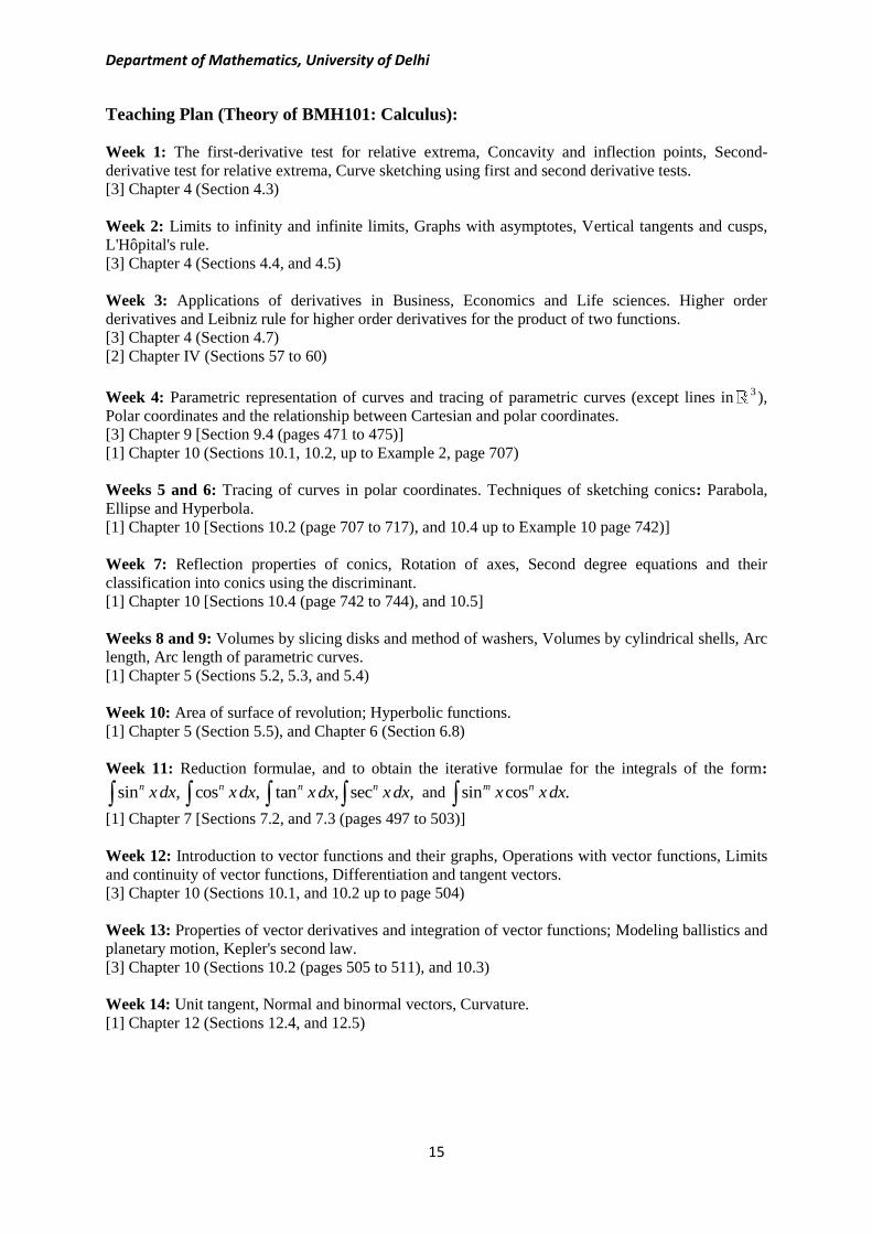
Teaching Plan (Theory of BMH101: Calculus):
Week 1: The first-derivative test for relative extrema, Concavity and inflection points, Second-
derivative test for relative extrema, Curve sketching using first and second derivative tests.
[3] Chapter 4 (Section 4.3)
Week 2: Limits to infinity and infinite limits, Graphs with asymptotes, Vertical tangents and cusps,
L'Hôpital's rule.
[3] Chapter 4 (Sections 4.4, and 4.5)
Week 3: Applications of derivatives in Business, Economics and Life sciences. Higher order
derivatives and Leibniz rule for higher order derivatives for the product of two functions.
[3] Chapter 4 (Section 4.7)
[2] Chapter IV (Sections 57 to 60)
Week 4: Parametric representation of curves and tracing of parametric curves (except lines in3),
Polar coordinates and the relationship between Cartesian and polar coordinates.
[3] Chapter 9 [Section 9.4 (pages 471 to 475)]
[1] Chapter 10 (Sections 10.1, 10.2, up to Example 2, page 707)
Weeks 5 and 6: Tracing of curves in polar coordinates. Techniques of sketching conics: Parabola,
Ellipse and Hyperbola.
[1] Chapter 10 [Sections 10.2 (page 707 to 717), and 10.4 up to Example 10 page 742)]
Week 7: Reflection properties of conics, Rotation of axes, Second degree equations and their
classification into conics using the discriminant.
[1] Chapter 10 [Sections 10.4 (page 742 to 744), and 10.5]
Weeks 8 and 9: Volumes by slicing disks and method of washers, Volumes by cylindrical shells, Arc
length, Arc length of parametric curves.
[1] Chapter 5 (Sections 5.2, 5.3, and 5.4)
Week 10: Area of surface of revolution; Hyperbolic functions.
[1] Chapter 5 (Section 5.5), and Chapter 6 (Section 6.8)
Week 11: Reduction formulae, and to obtain the iterative formulae for the integrals of the form:
sin , cos , tan , sec ,n n n nx dx x dx x dx x dx and sin cos .m nx x dx
[1] Chapter 7 [Sections 7.2, and 7.3 (pages 497 to 503)]
Week 12: Introduction to vector functions and their graphs, Operations with vector functions, Limits
and continuity of vector functions, Differentiation and tangent vectors.
[3] Chapter 10 (Sections 10.1, and 10.2 up to page 504)
Week 13: Properties of vector derivatives and integration of vector functions; Modeling ballistics and
planetary motion, Kepler's second law.
[3] Chapter 10 (Sections 10.2 (pages 505 to 511), and 10.3)
Week 14: Unit tangent, Normal and binormal vectors, Curvature.
[1] Chapter 12 (Sections 12.4, and 12.5)

Department of Mathematics, University of Delhi
16
BMH102: Algebra
Total Marks: 100 (Theory: 75, Internal Assessment: 25)
Workload: 5 Lectures (per week), 1 Tutorial (per week per student)
Duration: 14 Weeks (70 Hrs.) Examination: 3 Hrs.
Course Objectives: The primary objective of this course is to introduce the basic tools of
theory of equations, complex numbers, number theory and matrices to understand their linkage
to the real-world problems. Perform matrix algebra with applications to Computer Graphics.
Course Learning Outcomes: This course will enable the students to:
i) Employ De Moivre’s theorem in a number of applications to solve numerical problems.
ii) Apply Euclid’s algorithm and backwards substitution to find greatest common divisor.
iii) Recognize consistent and inconsistent systems of linear equations by the row echelon
form of the augmented matrix, using rank.
iv) Find eigenvalues and corresponding eigenvectors for a square matrix.
Course Contents:
Unit 1: Theory of Equations and Complex Numbers (Lectures: 20)
Elementary theorems on the roots of an equation, Polynomials, The remainder and factor
theorem, Synthetic division, Factored form of a polynomial, The Fundamental theorem of
algebra, Relations between the roots and the coefficients of polynomial equations, Imaginary
roots occur in pairs, Integral and rational roots; Polar representation of complex numbers, The
nth roots of unity, De Moivre’s theorem for integer and rational indices and its applications.
Unit 2: Equivalence Relations and Functions (Lectures: 10)
Equivalence relations, Functions, Composition of functions, Invertibility and inverse of
functions, One-to-one correspondence and the cardinality of a set.
Unit 3: Basic Number Theory (Lectures: 10)
The division algorithm, Divisibility and the Euclidean algorithm, The fundamental theorem
of arithmetic, Modular arithmetic and basic properties of congruences; Principles of
mathematical induction and well ordering principle.
Unit 4: Row Echelon Form of Matrices and Applications (Lectures: 30)
Systems of linear equations, Row reduction and echelon forms, Vector equations, The matrix
equation Ax = b, Solution sets of linear systems, Linear independence, The rank of a matrix and
applications; Introduction to linear transformations, The matrix of a linear transformation;
Matrix operations, The inverse of a matrix, Characterizations of invertible matrices,
Applications to Computer Graphics, Eigenvectors and eigenvalues, The characteristic equation
and the Cayley-Hamilton theorem.
References:
1. Andreescu, Titu & Andrica Dorin. (2014). Complex Numbers from A to...Z.
(2nd ed.). Birkhäuser.
Department of Mathematics, University of Delhi
17
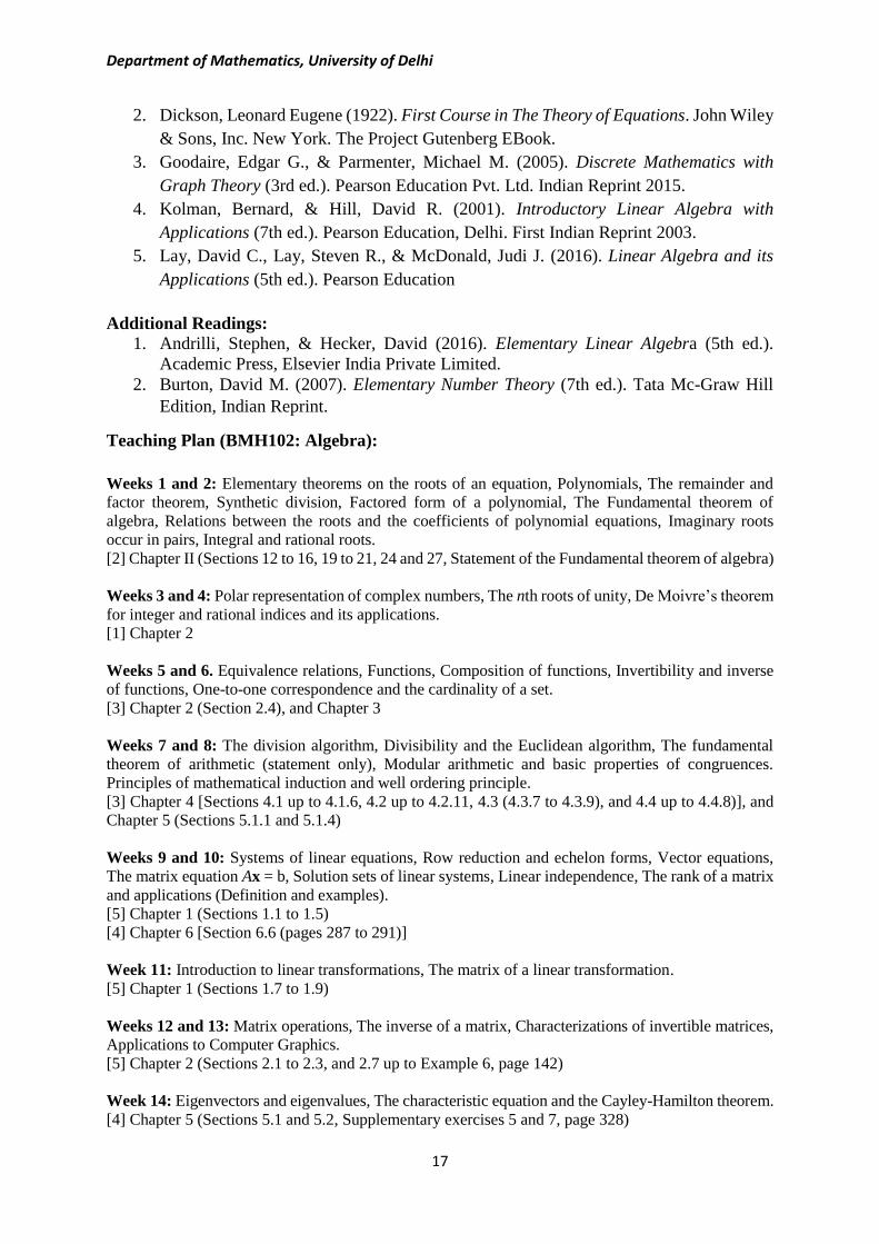
2. Dickson, Leonard Eugene (1922). First Course in The Theory of Equations. John Wiley
& Sons, Inc. New York. The Project Gutenberg EBook.
3. Goodaire, Edgar G., & Parmenter, Michael M. (2005). Discrete Mathematics with
Graph Theory (3rd ed.). Pearson Education Pvt. Ltd. Indian Reprint 2015.
4. Kolman, Bernard, & Hill, David R. (2001). Introductory Linear Algebra with
Applications (7th ed.). Pearson Education, Delhi. First Indian Reprint 2003.
5. Lay, David C., Lay, Steven R., & McDonald, Judi J. (2016). Linear Algebra and its
Applications (5th ed.). Pearson Education
Additional Readings:
1. Andrilli, Stephen, & Hecker, David (2016). Elementary Linear Algebra (5th ed.).
Academic Press, Elsevier India Private Limited.
2. Burton, David M. (2007). Elementary Number Theory (7th ed.). Tata Mc-Graw Hill
Edition, Indian Reprint.
Teaching Plan (BMH102: Algebra):
Weeks 1 and 2: Elementary theorems on the roots of an equation, Polynomials, The remainder and
factor theorem, Synthetic division, Factored form of a polynomial, The Fundamental theorem of
algebra, Relations between the roots and the coefficients of polynomial equations, Imaginary roots
occur in pairs, Integral and rational roots.
[2] Chapter II (Sections 12 to 16, 19 to 21, 24 and 27, Statement of the Fundamental theorem of algebra)
Weeks 3 and 4: Polar representation of complex numbers, The nth roots of unity, De Moivre’s theorem
for integer and rational indices and its applications.
[1] Chapter 2
Weeks 5 and 6. Equivalence relations, Functions, Composition of functions, Invertibility and inverse
of functions, One-to-one correspondence and the cardinality of a set.
[3] Chapter 2 (Section 2.4), and Chapter 3
Weeks 7 and 8: The division algorithm, Divisibility and the Euclidean algorithm, The fundamental
theorem of arithmetic (statement only), Modular arithmetic and basic properties of congruences.
Principles of mathematical induction and well ordering principle. [3] Chapter 4 [Sections 4.1 up to 4.1.6, 4.2 up to 4.2.11, 4.3 (4.3.7 to 4.3.9), and 4.4 up to 4.4.8)], and
Chapter 5 (Sections 5.1.1 and 5.1.4)
Weeks 9 and 10: Systems of linear equations, Row reduction and echelon forms, Vector equations,
The matrix equation Ax = b, Solution sets of linear systems, Linear independence, The rank of a matrix
and applications (Definition and examples).
[5] Chapter 1 (Sections 1.1 to 1.5)
[4] Chapter 6 [Section 6.6 (pages 287 to 291)]
Week 11: Introduction to linear transformations, The matrix of a linear transformation.
[5] Chapter 1 (Sections 1.7 to 1.9)
Weeks 12 and 13: Matrix operations, The inverse of a matrix, Characterizations of invertible matrices,
Applications to Computer Graphics.
[5] Chapter 2 (Sections 2.1 to 2.3, and 2.7 up to Example 6, page 142)
Week 14: Eigenvectors and eigenvalues, The characteristic equation and the Cayley-Hamilton theorem.
[4] Chapter 5 (Sections 5.1 and 5.2, Supplementary exercises 5 and 7, page 328)

Department of Mathematics, University of Delhi
18
Semester II
BMH203: Real Analysis
Total Marks: 100 (Theory: 75, Internal Assessment: 25)
Workload: 5 Lectures (per week), 1 Tutorial (per week per student)
Duration: 14 Weeks (70 Hrs.) Examination: 3 Hrs.
Course Objectives: The course will develop a deep and rigorous understanding of real line
and of defining terms to prove the results about convergence and divergence of sequences and
series of real numbers. These concepts has vide range of applications in real life scenario.
Course Learning Outcomes: This course will enable the students to:
i) Understand many properties of the real line and learn to define sequence in terms of
functions from to a subset of .
ii) Recognize bounded, convergent, divergent, Cauchy and monotonic sequences and to
calculate their limit superior, limit inferior, and the limit of a bounded sequence.
iii) Apply the ratio, root, alternating series and limit comparison tests for convergence and
absolute convergence of an infinite series of real numbers.
Course Contents:
Unit 1: Real Number System (Lectures: 10)
Algebraic and order properties of , Absolute value of a real number; Bounded above and
bounded below sets, Supremum and infimum of a nonempty subset of .
Unit 2: Properties of (Lectures: 10)
The completeness property of , Archimedean property, Density of rational numbers in ;
Definition and types of intervals, Nested intervals property; Neighborhood of a point in ,
Open and closed sets in .
Unit 3: Sequences in (Lectures: 25)
Convergent sequence, Limit of a sequence, Bounded sequence, Limit theorems, Monotone
sequences, Monotone convergence theorem, Subsequences, Bolzano-Weierstrass theorem for
sequences, Limit superior and limit inferior for bounded sequence, Cauchy sequence, Cauchy’s
convergence criterion.
Unit 4: Infinite Series (Lectures: 25)
Convergence and divergence of infinite series of real numbers, Necessary condition for
convergence, Cauchy criterion for convergence; Tests for convergence of positive term series:
Integral test, Basic comparison test, Limit comparison test, D’Alembert’s ratio test, Cauchy’s
nth root test; Alternating series, Leibniz test, Absolute and conditional convergence.
References:
1. Bartle, Robert G., & Sherbert, Donald R. (2015). Introduction to Real Analysis
(4th ed.). Wiley India Edition. New Delhi.

Department of Mathematics, University of Delhi
19
2. Bilodeau, Gerald G., Thie, Paul R., & Keough, G. E. (2010). An Introduction to
Analysis (2nd ed.). Jones and Bartlett India Pvt. Ltd. Student Edition. Reprinted 2015.
3. Denlinger, Charles G. (2011). Elements of Real Analysis. Jones and Bartlett India Pvt.
Ltd. Student Edition. Reprinted 2015.
Additional Readings:
1. Ross, Kenneth A. (2013). Elementary Analysis: The theory of calculus (2nd ed.).
Undergraduate Texts in Mathematics, Springer. Indian Reprint.
2. Thomson, Brian S., Bruckner, Andrew. M., & Bruckner, Judith B. (2001). Elementary
Real Analysis. Prentice Hall.
Teaching Plan (Theory of BMH203: Real Analysis):
Weeks 1 and 2: Algebraic and order properties of . Absolute value of a real number; Bounded above
and bounded below sets, Supremum and infimum of a nonempty subset of .
[1] Chapter 2 [Sections 2.1, 2.2 (2.2.1 to 2.2.6), and 2.3 (2.3.1 to 2.3.5)]
Weeks 3 and 4: The completeness property of , Archimedean property, Density of rational numbers
in ; Definition and types of intervals, Nested intervals property; Neighborhood of a point in , Open
and closed sets in .
[1] Chapter 2 [Sections 2.3 (2.3.6), 2.4 (2.4.3 to 2.4.9), and 2.5 up to Theorem 2.5.3]
[1] Chapter 11 [Section 11.1 (11.1.1 to 11.1.3)]
Weeks 5 and 6: Sequences and their limits, Bounded sequence, Limit theorems.
[1] Chapter 3 (Sections 3.1 and 3.2)
Week 7: Monotone sequences, Monotone convergence theorem and applications.
[1] Chapter 3 (Section 3.3)
Week 8: Subsequences and statement of the Bolzano-Weierstrass theorem. Limit superior and limit
inferior for bounded sequence of real numbers with illustrations only. [1] Chapter 3 [Section 3.4 (3.4.1 to 3.4.12), except 3.4.4, 3.4.7, 3.4.9 and 3.4.11]
Week 9: Cauchy sequences of real numbers and Cauchy’s convergence criterion.
[1] Chapter 3 [Section 3.5 (3.5.1 to 3.5.6)]
Week 10: Convergence and divergence of infinite series, Sequence of partial sums of infinite series,
Necessary condition for convergence, Cauchy criterion for convergence of series.
[3] Chapter 8 (Section 8.1)
Weeks 11 and 12: Tests for convergence of positive term series: Integral test statement and
convergence of p-series, Basic comparison test, Limit comparison test with applications, D’Alembert’s
ratio test and Cauchy’s nth root test.
[3] Chapter 8 (Section 8.2 up to 8.2.19)
Weeks 13 and 14: Alternating series, Leibniz test, Absolute and conditional convergence.
[2] Chapter 6 (Section 6.2)

Department of Mathematics, University of Delhi
20
BMH204: Differential Equations
Total Marks: 150 (Theory: 75, Internal Assessment: 25 and Practical: 50)
Workload: 4 Lectures (per week), 4 Practicals (per week per student)
Duration: 14 Weeks (56 Hrs. Theory + 56 Hrs. Practical) Examination: 3 Hrs.
Course Objectives: The main objectives of this course are to introduce the students to the
exciting world of Differential Equations, Mathematical Modeling and their applications.
Course Learning Outcomes: The course will enable the students to:
i) Formulate Differential Equations for various Mathematical models.
ii) Solve first order non-linear differential equation and linear differential equations of
higher order using various techniques.
iii) Apply these techniques to solve and analyze various mathematical models.
Course Contents:
Unit 1: Differential Equations and Mathematical Modeling (Lectures: 12)
Differential equations and mathematical models, Order and degree of a differential equation,
Exact differential equations and integrating factors of first order differential equations,
Reducible second order differential equations, Application of first order differential equations
to equations to acceleration-velocity model, Growth and decay model.
Unit 2: Population Growth Models (Lectures: 12)
Introduction to compartmental models, Lake pollution model (with case study of Lake Burley
Griffin), Drug assimilation into the blood (case of a single cold pill, case of a course of cold
pills, case study of alcohol in the bloodstream), Exponential growth of population, Limited
growth of population, Limited growth with harvesting.
Unit 3: Second and Higher Order Differential Equations (Lectures: 20)
General solution of homogeneous equation of second order, Principle of superposition for a
homogeneous equation; Wronskian, its properties and applications, Linear homogeneous and
non-homogeneous equations of higher order with constant coefficients, Euler’s equation,
Method of undetermined coefficients, Method of variation of parameters, Applications of
second order differential equations to mechanical vibrations.
Unit 4: Analysis of Mathematical Models (Lectures: 12)
Interacting population models, Epidemic model of influenza and its analysis, Predator-prey
model and its analysis, Equilibrium points, Interpretation of the phase plane, Battle model and
its analysis.
References:
1. Barnes, Belinda & Fulford, Glenn R. (2015). Mathematical Modelling with Case
Studies, Using Maple and MATLAB (3rd ed.). CRC Press, Taylor & Francis Group.
2. Edwards, C. Henry, Penney, David E., & Calvis, David T. (2015). Differential Equation
and Boundary Value Problems: Computing and Modeling (5th ed.). Pearson Education.
3. Ross, Shepley L. (2004). Differential Equations (3rd ed.). John Wiley & Sons. India

Department of Mathematics, University of Delhi
21
Practical /Lab work to be performed in a Computer Lab:
Modeling of the following problems using Mathematica /MATLAB/Maple/Maxima/Scilab etc.
1. Plotting of second and third order respective solution family of differential equation.
2. Growth and decay model (exponential case only).
3. (a) Lake pollution model (with constant/seasonal flow and pollution concentration).
(b) Case of single cold pill and a course of cold pills.
(c) Limited growth of population (with and without harvesting).
4. (a) Predatory-prey model (basic volterra model, with density dependence, effect of
DDT, two prey one predator).
(b) Epidemic model of influenza (basic epidemic model, contagious for life, disease
with carriers).
(c) Battle model (basic battle model, jungle warfare, long range weapons).
5. Plotting of recursive sequences, and study the convergence.
6. Find a value m that will make the following inequality holds for all :n m
3 3
3 7
( ) 0.5 1 10 , ( ) 1 10 ,
( ) (0.9) 10 , ( ) 2 ! 10 , etc.
n n
n n
i ii n
iii iv n
7. Verify the Bolzano-Weierstrass theorem through plotting of sequences and hence identify
convergent subsequences from the plot.
8. Study the convergence/divergence of infinite series of real numbers by plotting their
sequences of partial sum.
9. Cauchy’s root test by plotting nth roots.
10. D’Alembert’s ratio test by plotting the ratio of nth and (n+1)th term of the given series of
positive terms.
11. For the following sequences na , given 1 2 , 10 , 0,1,2, ; 1,2,3,k jp k j
Find m such that 2 2( ) , ( ) ,m p m m p mi a a ii a a where na is given as:
1
2
1 1 1 1 ( 1)( ) , ( ) , ( ) 1
2 3
( 1) 1 1( ) , ( ) 2 , ( ) 1
2! !
n
nn
na b c
n n n
d e n fn n
12. For the following series na , calculate
11( ) , ( ) , for 10 , 1,2,3,n jn
n
n
ai ii a n j
a
,
and identify the convergent series, where na is given as:
3 21
2
3
2 2
1 1 1 1 !( ) , ( ) , ( ) , ( ) 1 , ( )
5 1 1 1 1( ) , ( ) , ( ) , ( ) cos , ( ) , ( )
3 2 log (log )1
nn
n
n
na b c d e
n n n nn
nf g h i n j k
n n n n n nn

Department of Mathematics, University of Delhi
22
Teaching Plan (Theory of BMH204: Differential Equations):
Weeks 1 and 2: Differential equations and mathematical models, Order and degree of a differential
equation, Exact differential equations and integrating factors of first order differential equations,
Reducible second order differential equations.
[2] Chapter 1 (Sections 1.1, and 1.6)
[3] Chapter 2.
Week 3: Application of first order differential equations to equations to acceleration-velocity model,
Growth and decay model.
[2] Chapter 1 (Section 1.4, pages 35 to 38), and Chapter 2 (Section 2.3)
[3] Chapter 3 (Section 3.3, A and B with Examples 3.8, 3.9)
Week 4: Introduction to compartmental models, Lake pollution model (with case study of Lake Burley
Griffin).
[1] Chapter 2 (Sections 2.1, 2.5, and 2.6)
Week 5: Drug assimilation into the blood (case of a single cold pill, case of a course of cold pills, Case
study of alcohol in the bloodstream).
[1] Chapter 2 (Sections 2.7, and 2.8)
Week 6: Exponential growth of population, Density dependent growth, Limited growth with
harvesting.
[1] Chapter 3 (Sections 3.1 to 3.3)
Weeks 7 to 9: General solution of homogeneous equation of second order, Principle of superposition
for a homogeneous equation; Wronskian, its properties and applications; Linear homogeneous and non-
homogeneous equations of higher order with constant coefficients; Euler’s equation.
[2] Chapter 3 (Sections 3.1 to 3.3)
Weeks 10 and 11: Method of undetermined coefficients, Method of variation of parameters;
Applications of second order differential equations to mechanical vibrations.
[2] Chapter 3 (Sections 3.4 (pages 172 to 177), and 3.5)
Weeks 12 to 14: Interacting population models, Epidemic model of influenza and its analysis, Predator-
prey model and its analysis, Equilibrium points, Interpretation of the phase plane, Battle model and its
analysis.
[1] Chapter 5 (Sections 5.1, 5.2, 5.4, and 5.9), and Chapter 6 (Sections 6.1 to 6.4).

Department of Mathematics, University of Delhi
23
Semester III
BMH305: Theory of Real Functions
Total Marks: 100 (Theory: 75, Internal Assessment: 25)
Workload: 5 Lectures (per week), 1 Tutorial (per week per student)
Duration: 14 Weeks (70 Hrs.) Examination: 3 Hrs. Course Objectives: It is a basic course on the study of real valued functions that would develop
an analytical ability to have a more matured perspective of the key concepts of calculus,
namely, limits, continuity, differentiability and their applications.
Course Learning Outcomes: This course will enable the students to learn:
i) To have a rigorous understanding of the concept of limit of a function.
ii) The geometrical properties of continuous functions on closed and bounded intervals.
iii) The applications of mean value theorem and Taylor’s theorem.
Course Contents:
Unit 1: Limits of Functions (Lectures: 15)
Limits of functions ( approach), Sequential criterion for limits, Divergence criteria, Limit
theorems, One-sided limits, Infinite limits and limits at infinity.
Unit 2: Continuous Functions and their Properties (Lectures: 25)
Continuous functions, Sequential criterion for continuity and discontinuity, Algebra of
continuous functions, Properties of continuous functions on closed and bounded intervals;
Uniform continuity, Non-uniform continuity criteria, Uniform continuity theorem.
Unit 3: Derivability and its Applications (Lectures: 20)
Differentiability of a function, Algebra of differentiable functions, Carathéodory’s theorem and
chain rule; Relative extrema, Interior extremum theorem, Rolle’s theorem, Mean- value
theorem and its applications, Intermediate value property of derivatives - Darboux’s theorem.
Unit 4: Taylor’s Theorem and its Applications (Lectures: 10)
Taylor polynomial, Taylor’s theorem with Lagrange form of remainder, Application of
Taylor’s theorem in error estimation; Relative extrema, and to establish a criterion for convexity;
Taylor’s series expansions of , sinxe x and cos .x
Reference:
1. Bartle, Robert G., & Sherbert, Donald R. (2015). Introduction to Real Analysis (4th
ed.). Wiley India Edition. New Delhi.
Additional Readings:
1. Ghorpade, Sudhir R. & Limaye, B. V. (2006). A Course in Calculus and Real Analysis.
Undergraduate Texts in Mathematics, Springer (SIE). First Indian reprint.
2. Mattuck, Arthur. (1999). Introduction to Analysis, Prentice Hall.
3. Ross, Kenneth A. (2013). Elementary Analysis: The theory of calculus (2nd ed.).
Undergraduate Texts in Mathematics, Springer. Indian Reprint.

Department of Mathematics, University of Delhi
24
Teaching Plan (Theory of BMH305: Theory of Real Functions):
Week 1: Definition of the limit, Sequential criterion for limits, Criterion for non-existence of limit.
[1] Chapter 4 (Section 4.1)
Week 2: Algebra of limits of functions with illustrations and examples, Squeeze theorem.
[1] Chapter 4 (Section 4.2)
Week 3: Definition and illustration of the concepts of one-sided limits, Infinite limits and limits at
infinity.
[1] Chapter 4 (Section 4.3)
Weeks 4 and 5: Definitions of continuity at a point and on a set, Sequential criterion for continuity,
Algebra of continuous functions, Composition of continuous functions.
[1] Chapter 5 (Sections 5.1, and 5.2)
Weeks 6 and 7: Various properties of continuous functions defined on an interval, viz., Boundedness
theorem, Maximum-minimum theorem, Statement of the location of roots theorem, Intermediate
value theorem and the preservation of intervals theorem.
[1] Chapter 5 (Section 5.3)
Week 8: Definition of uniform continuity, Illustration of non-uniform continuity criteria, Uniform
continuity theorem.
[1] Chapter 5 [Section 5.4 (5.4.1 to 5.4.3)]
Weeks 9 and 10: Differentiability of a function, Algebra of differentiable functions, Carathéodory’s
theorem and chain rule.
[1] Chapter 6 [Section 6.1 (6.1.1 to 6.1.7)]
Weeks 11 and 12: Relative extrema, Interior extremum theorem, Mean value theorem and its
applications, Intermediate value property of derivatives- Darboux’s theorem.
[1] Chapter 6 (Section 6.2)
Weeks 13 and 14: Taylor polynomial, Taylor’s theorem and its applications, Taylor’s series
expansions of , sinxe x and cos .x
[1] Chapter 6 (Sections 6.4.1 to 6.4.6), and Chapter 9 (Example 9.4.14, page 286)

Department of Mathematics, University of Delhi
25
BMH306: Group Theory-I
Total Marks: 100 (Theory: 75, Internal Assessment: 25)
Workload: 5 Lectures (per week), 1 Tutorial (per week per student)
Duration: 14 Weeks (70 Hrs.) Examination: 3 Hrs.
Course Objectives: The objective of the course is to introduce the fundamental theory of
groups and their homomorphisms. Symmetric groups and group of symmetries are also studied
in detail. Fermat’s Little theorem as a consequence of the Lagrange’s theorem on finite groups.
Course Learning Outcomes: The course will enable the students to:
i) Recognize the mathematical objects that are groups, and classify them as abelian, cyclic
and permutation groups, etc;
ii) Link the fundamental concepts of Groups and symmetrical figures;
iii) Analyze the subgroups of cyclic groups;
iv) Explain the significance of the notion of cosets, normal subgroups, and factor groups.
Course Contents:
Unit 1: Groups and its Elementary Properties (Lectures: 10)
Symmetries of a square, The Dihedral groups, Definition and examples of groups including
permutation groups and quaternion groups (illustration through matrices), Elementary
properties of groups.
Unit 2: Subgroups and Cyclic Groups (Lectures: 15)
Subgroups and examples of subgroups, Centralizer, Normalizer, Center of a group, Product of
two subgroups; Properties of cyclic groups, Classification of subgroups of cyclic groups.
Unit 3: Permutation Groups and Lagrange’s Theorem (Lectures: 25)
Cycle notation for permutations, Properties of permutations, Even and odd permutations,
alternating groups; Properties of cosets, Lagrange’s theorem and consequences including
Fermat’s Little theorem; Normal subgroups, factor groups, Cauchy’s theorem for finite abelian
groups.
Unit 4: Group Homomorphisms (Lectures: 20)
Group homomorphisms, Properties of homomorphisms, Group isomorphisms, Cayley’s
theorem, Properties of isomorphisms, First, Second and Third isomorphism theorems for
groups.
Reference:
1. Gallian, Joseph. A. (2013). Contemporary Abstract Algebra (8th ed.). Cengage
Learning India Private Limited, Delhi. Fourth impression, 2015.
Additional Reading:
1. Rotman, Joseph J. (1995). An Introduction to The Theory of Groups (4th ed.). Springer
Verlag, New York.

Department of Mathematics, University of Delhi
26
Teaching Plan (BMH306: Group Theory-I):
Week 1: Symmetries of a square, The Dihedral groups, Definition and examples of groups including
permutation groups and quaternion groups (illustration through matrices)
[1] Chapter 1
Week 2: Definition and examples of groups, Elementary properties of groups.
[1] Chapter 2
Week 3: Subgroups and examples of subgroups, Centralizer, Normalizer, Center of a Group, Product
of two subgroups.
[1] Chapter 3
Weeks 4 and 5: Properties of cyclic groups. Classification of subgroups of cyclic groups.
[1] Chapter 4
Weeks 6 and 7: Cycle notation for permutations, Properties of permutations, Even and odd
permutations, Alternating group.
[1] Chapter 5 (up to page 110)
Weeks 8 and 9: Properties of cosets, Lagrange’s theorem and consequences including Fermat’s Little
theorem.
[1] Chapter 7 (up to Example 6, page 150)
Week 10: Normal subgroups, Factor groups, Cauchy’s theorem for finite abelian groups.
[1] Chapters 9 (Theorem 9.1, 9.2, 9.3 and 9.5, and Examples 1 to 12)
Weeks 11 and 12: Group homomorphisms, Properties of homomorphisms, Group isomorphisms,
Cayley’s theorem.
[1] Chapter 10 (Theorems 10.1 and 10.2, Examples 1 to 11)
[1] Chapter 6 (Theorem 6.1, and Examples 1 to 8)
Weeks 13 and 14: Properties of isomorphisms, First, Second and Third isomorphism theorems.
[1] Chapter 6 (Theorems 6.2 and 6.3, and Examples 1 to 8)
[1] Chapter 10 (Theorems 10.3, 10.4, Examples 12 to 14, and Exercises 41 and 42 for second and third
isomorphism theorems for groups)

Department of Mathematics, University of Delhi
27
BMH307: Multivariate Calculus
Total Marks: 150 (Theory: 75, Internal Assessment: 25 and Practical: 50)
Workload: 4 Lectures (per week), 4 Practicals (per week per student)
Duration: 14 Weeks (56 Hrs. Theory + 56 Hrs. Practical) Examination: 3 Hrs.
Course Objectives: To understand the extension of the studies of single variable differential
and integral calculus to functions of two or more independent variables. Also, the emphasis
will be on the use of Computer Algebra Systems by which these concepts may be analyzed and
visualized to have a better understanding.
Course Learning Outcomes: This course will enable the students to learn:
i) The conceptual variations when advancing in calculus from one variable to
multivariable discussions.
ii) Inter-relationship amongst the line integral, double and triple integral formulations.
iii) Applications of multi variable calculus tools in physics, economics, optimization, and
understanding the architecture of curves and surfaces in plane and space etc.
Course Contents:
Unit 1: Calculus of Functions of Several Variables (Lectures: 20)
Functions of several variables, Level curves and surfaces, Limits and continuity, Partial
differentiation, Higher order partial derivative, Tangent planes, Total differential and
differentiability, Chain rule, Directional derivatives, The gradient, Maximal and normal
property of the gradient, Tangent planes and normal lines.
Unit 2: Extrema of Functions of Two Variables and Properties of Vector Field (Lectures: 8)
Extrema of functions of two variables, Method of Lagrange multipliers, Constrained
optimization problems; Definition of vector field, Divergence and curl.
Unit 3: Double and Triple Integrals (Lectures: 16)
Double integration over rectangular and nonrectangular regions, Double integrals in polar co-
ordinates, Triple integral over a parallelepiped and solid regions, Volume by triple integrals,
triple integration in cylindrical and spherical coordinates, Change of variables in double and
triple integrals.
Unit 4: Green's, Stokes' and Gauss Divergence Theorem (Lectures: 12)
Line integrals, Applications of line integrals: Mass and Work, Fundamental theorem for line
integrals, Conservative vector fields, Green's theorem, Area as a line integral; Surface integrals,
Stokes' theorem, The Gauss divergence theorem.
References:
1. Strauss, Monty J., Bradley, Gerald L., & Smith, Karl J. (2007). Calculus (3rd ed.).
Dorling Kindersley (India) Pvt. Ltd. (Pearson Education). Delhi. Indian Reprint 2011.
2. Marsden, J. E., Tromba, A., & Weinstein, A. (2004). Basic Multivariable Calculus.
Springer (SIE). First Indian Reprint.

Department of Mathematics, University of Delhi
28
Practical/Lab work to be performed in Computer Lab.
List of practicals to be done using Mathematica / MATLAB / Maple/Maxima/Scilab, etc.
1. Let be any function and L be any real number. For given a and , find a
such that for all x satisfying the inequality holds.
For example:
(a)
(b)
(c)
(d)
2. Discuss the limit of the following functions when x tends to 0:
3. Discuss the limit of the following functions when x tends to infinity:
4. Discuss the continuity of the functions at x = 0 in the Practical 2.
5. Illustrate the geometric meaning of Rolle’s theorem of the following functions on the
given interval: (i) on [-2, 2]; (ii) on [3, 5] etc.
6. Illustrate the geometric meaning of Lagrange’s mean value theorem of the following
functions on the given interval:
(i) on [1/2, 2]; (ii) on [0, 1/2]; (iii) on [2, 5] etc.
7. Visualization by creating graphs: Taylor’s polynomials – approximated up to certain
degrees.
8. Draw the following surfaces and find level curves at the given heights:
(a)
(b)
(c)
(d)
(e)
( )f x 0
0 0 | | ,x a 0 | ( ) |f x l
( ) 1, 5, 4, 0.01f x x L a
( ) 1, 1, 4, 0.1f x x L a
2( ) , 4, 2, 0.5f x x L a
1( ) , 1, 1, 0.1f x L a
x
21 1 1 1 1 1, sin , cos , sin , cos , sin ,
1 1( ), [ ] greatest integer function, sin .
n
x x xx x x x x x
n x xx x
1
2
2
1 1 1, sin , , , sin , ( 0 )
1
xxx ax b
e e x a cx x x x cx dx e
3 4x x 4 3( 3) ( 5)x x
log x ( 1)( 2)x x x 22 7 10x x
2 2( , ) 10 ; 1, 6, 9f x y x y z z z 2 2( , ) ; 1, 6, 9f x y x y z z z
3( , ) ; 1, 6f x y x y z z 2
2( , ) ; 1, 5, 84
yf x y x z z z
2 2( , ) 4 ; 0, 1, 6, 9f x y x y z z z z

Department of Mathematics, University of Delhi
29
9. Draw the following surfaces and discuss whether limit exits or not as (x, y)
approaches to the given points. Find the limit, if it exists:
(i)
(ii)
(iii)
(iv)
(v)
(vi)
10. Draw the tangent plane to the following surfaces at the given point:
(i)
(ii)
(iii)
(iv) 1tan at (1, 3, 3) and (2, 2, 4)z x
(v)
11. Use an incremental approximation to estimate the following functions at the given
point and compare it with calculated value:
(i)
(ii)
(iii)
12. Find critical points and identify relative maxima, relative minima or saddle points to the
following surfaces, if it exists:
(i) ; (ii) ; (iii) ; (iv) .
13. Draw the following regions D and check whether these regions are of Type I or Type II:
(i)
(ii)
(iii)
(iv) The region D is bounded by and the line y = x.
(v)
( , ) ; ( , ) (0,0) and ( , ) (1,3)x y
f x y x y x yx y
2 2( , ) ; ( , ) (0,0) and ( , ) (2,1)
x yf x y x y x y
x y
( , ) ( ) ; ( , ) (1,1) and ( , ) (1,0)xyf x y x y e x y x y
( , ) ; ( , ) (0,0) and ( , ) (1,0)xyf x y e x y x y 2
2 2( , ) ; ( , ) (0,0)
x yf x y x y
x y
2 2
2 2( , ) ; ( , ) (0,0) and ( , ) (2,1)
x yf x y x y x y
x y
2 2( , ) at (3,1, 10)f x y x y
2 2( , ) 10 at (2,2,2)f x y x y
2 2 2 9 at (3,0,0)x y z
2log | | at ( 3, 2,0)z x y
4 4( , ) 3 2 at (1.01,2.03)f x y x y
5 3( , ) 2 at (0.98,1.03)f x y x y
( , ) at (1.01,0.98)xyf x y e
2 2z x y 2 21z x y 2 2z y x 2 4z x y
{( , ) : 0 2,1 }xD x y x y e 2{( , ) : log 2,1 }D x y y x y e
3{( , ) : 0 1, 1}D x y x x y 2 2y x
{( , ) : 0 ,sin cos }4
D x y x x y x

Department of Mathematics, University of Delhi
30
Teaching Plan (Theory of BMH307: Multivariate Calculus): Week 1: Definition of functions of several variables, Graphs of functions of two variables – Level
curves and surfaces, Limits and continuity of functions of two variables.
[1] Chapter 11 (Sections 11.1 and 11.2)
Week 2: Partial differentiation, and partial derivative as slope and rate, Higher order partial derivatives.
Tangent planes, incremental approximation, Total differential.
[1] Chapter 11 (Sections 11.3 and 11.4)
Week 3: Differentiability, Chain rule for one parameter, Two and three independent parameters.
[1] Chapter 11 (Sections 11.4 and 11.5)
Week 4: Directional derivatives, The gradient, Maximal and normal property of the gradient, Tangent
planes and normal lines.
[1] Chapter 11 (Section 11.6)
Week 5: First and second partial derivative tests for relative extrema of functions of two variables,
and absolute extrema of continuous functions.
[1] Chapter 11 [Section 11.7 (up to page 605)]
Week 6: Lagrange multipliers method for optimization problems with one constraint, Definition of
vector field, Divergence and curl.
[1] Chapter 11 [Section 11.8 (pages 610-614)], Chapter13 (Section 13.1)
Week 7: Double integration over rectangular and nonrectangular regions.
[1] Chapter 12 (Sections 12.1 and 12.2)
Week 8: Double integrals in polar co-ordinates, and triple integral over a parallelepiped.
[1] Chapter 12 (Sections 12.3 and 12.4)
Week 9: Triple integral over solid regions, Volume by triple integrals, and triple integration in
cylindrical coordinates.
[1] Chapter 12 (Sections 12.4 and 12.5)
Week 10: Triple integration in spherical coordinates, Change of variables in double and triple integrals.
[1] Chapter 12 (Sections 12.5 and 12.6)
Week 11: Line integrals and its properties, applications of line integrals: mass and work.
[1] Chapter 13 (Section 13.2)
Week 12: Fundamental theorem for line integrals, Conservative vector fields and path independence.
[1] Chapter 13 (Section 13.3)
Week 13: Green's theorem for simply connected region, Area as a line integral, Definition of surface
integrals
[1] Chapter 13 [Sections 13.4 (pages 712 to 716), 13.5 (pages 723 to 726)]
Week 14: Stokes' theorem and the divergence theorem.
[1] Chapter 13 [Sections 13.6 (pages 733 to 737), 13.7 (pages 742 to 745)]
Note. To improve the problem solving ability, for similar kind of examples based upon the above
contents, the reference [2] may be consulted.

Department of Mathematics, University of Delhi
31
Skill Enhancement Paper
SEC-1: LaTeX and HTML
Total Marks: 100 (Theory: 38, Internal Assessment: 12 and Practical: 50)
Workload: 2 Lectures (per week), 4 Practicals (per week per student)
Duration: 14 Weeks (28 Hrs. Theory + 56 Hrs. Practical) Examination: 2 Hrs.
Course Objectives: The purpose of this course is to acquaint students with the latest
typesetting skills, which shall enable them to prepare high quality typesetting, beamer
presentation and webpages.
Course Learning Outcomes: After studying this course the student will be able to:
i) Typeset mathematical formulas, use nested list, tabular & array environments.
ii) Create or import graphics.
iii) Use beamer to create presentation and HTML to create a web page.
Course Contents:
Unit 1: Getting Started with LaTeX (Lectures: 6)
Introduction to TeX and LaTeX, Typesetting a simple document, Adding basic information to
a document, Environments, Footnotes, Sectioning and displayed material.
Unit 2: Mathematical Typesetting with LaTeX (Lectures: 6)
Accents and symbols, Mathematical Typesetting (Elementary and Advanced): Subscript/
Superscript, Fractions, Roots, Ellipsis, Mathematical Symbols, Arrays, Delimiters, Multiline
formulas, Spacing and changing style in math mode.
Unit 3: Graphics and Beamer Presentation in LaTeX (Lectures: 8) Graphics in LaTeX, Simple pictures using PS Tricks, Plotting of functions, Beamer
presentation.
Unit 4: HTML (Lectures: 8)
HTML basics, Creating simple web pages, Images and links, Design of web pages.
References:
1. Bindner, Donald & Erickson, Martin. (2011). A Student’s Guide to the Study, Practice,
and Tools of Modern Mathematics. CRC Press, Taylor & Francis Group, LLC.
2. Lamport, Leslie (1994). LaTeX: A Document Preparation System, User’s Guide and
Reference Manual (2nd ed.). Pearson Education. Indian Reprint.
Practical/Lab work to be performed in Computer Lab.
Practicals:
[1] Chapter 9 (Exercises 4 to 10), Chapter 10 (Exercises 1 to 4 and 6 to 9),
Chapter 11 (Exercises 1, 3, 4, and 5), and Chapter 15 (Exercises 5, 6 and 8 to 11).

Department of Mathematics, University of Delhi
32
Teaching Plan (Theory of SEC-1: LaTeX and HTML):
Weeks 1 to 3: Introduction to TeX and LaTeX, Typesetting a simple document, Adding basic
information to a document, Environments, Footnotes, Sectioning and displayed material.
[1] Chapter 9 (9.1 to 9.5)
[2] Chapter 2 (2.1 to 2.5)
Weeks 4 to 6: Accents of symbols, Mathematical typesetting (elementary and advanced):
subscript/superscript, Fractions, Roots, Ellipsis, Mathematical symbols, Arrays, Delimiters, Multiline
formulas, Spacing and changing style in math mode.
[1] Chapter 9 (9.6 and 9.7)
[2] Chapter 3 (3.1 to 3.3)
Weeks 7 and 8: Graphics in LaTeX, Simple pictures using PS Tricks, Plotting of functions.
[1] Chapter 9 (Section 9.8)
[1] Chapter 10 (10.1 to 10.3)
[2] Chapter 7 (7.1 and 7.2)
Weeks 9 and 10: Beamer presentation.
[1] Chapter 11 (Sections 11.1 to 11.4)
Weeks 11 and 12: HTML basics, Creating simple web pages.
[1] Chapter 15 (Sections 15.1 and 15.2)
Weeks 13 and 14: Adding images and links, Design of web pages.
[1] Chapter 15 (Sections 15.3 to 15.5)

Department of Mathematics, University of Delhi
33
Semester IV
BMH408: Partial Differential Equations
Total Marks: 150 (Theory: 75, Internal Assessment: 25 and Practical: 50)
Workload: 4 Lectures (per week), 4 Practicals (per week per student)
Duration: 14 Weeks (56 Hrs. Theory + 56 Hrs. Practical) Examination: 3 Hrs.
Course Objectives: The main objectives of this course are to teach students to form and solve
partial differential equations and use them in solving some physical problems.
Course Learning Outcomes: The course will enable the students to:
i) Formulate, classify and transform partial differential equations into canonical form.
ii) Solve linear and non-linear partial differential equations using various methods; and
apply these methods in solving some physical problems.
Course Contents:
Unit 1: First Order PDE and Method of Characteristics (Lectures: 12)
Introduction, Classification, Construction and geometrical interpretation of first order partial
differential equations (PDE), Method of characteristic and general solution of first order PDE,
Canonical form of first order PDE, Method of separation of variables for first order PDE.
Unit 2: Mathematical Models and Classification of 2nd Order Linear PDE (Lectures: 12)
Gravitational potential, Conservation laws and Burger’s equations, Classification of second
order PDE, Reduction to canonical forms, Equations with constant coefficients, General solution.
Unit 3: The Cauchy Problem and Wave Equations (Lectures: 16)
Mathematical modeling of vibrating string, vibrating membrane. Cauchy problem for second
order PDE, Homogeneous wave equation, Initial boundary value problems, Non-homogeneous
boundary conditions, Finite strings with fixed ends, Non-homogeneous wave equation, Goursat
problem.
Unit 4: Method of Separation of Variables (Lectures: 16)
Method of separation of variables for second order PDE, Vibrating string problem, Existence
and uniqueness of solution of vibrating string problem, Heat conduction problem, Existence
and uniqueness of solution of heat conduction problem, Non-homogeneous problem.
Reference:
1. Myint-U, Tyn & Debnath, Lokenath. (2007). Linear Partial Differential Equation for
Scientists and Engineers (4th ed.). Springer, Third Indian Reprint, 2013.
Additional Readings:
1. Sneddon, I. N. (2006). Elements of Partial Differential Equations, Dover
Publications. Indian Reprint.
2. Stavroulakis, Ioannis P & Tersian, Stepan A. (2004). Partial Differential Equations: An
Introduction with Mathematica and MAPLE (2nd ed.). World Scientific.

Department of Mathematics, University of Delhi
34
Practical /Lab work to be performed in a Computer Lab: Modeling of the following problems using Mathematica /MATLAB/ Maple/ Maxima/ Scilab etc.
1. Solution of Cauchy problem for first order PDE.
2. Plotting the characteristics for the first order PDE.
3. Plot the integral surfaces of a given first order PDE with initial data.
4. Solution of wave equation 𝜕2𝑢
𝜕𝑡2 = 𝑐2 𝜕2𝑢
𝜕𝑥2 for any two of the following associated conditions:
(a) 𝑢(𝑥, 0) = 𝜙(𝑥), 𝑢(𝑥, 0) = 𝜓(𝑥), 𝑥 ∈ ℝ, 𝑡 > 0
(b) 𝑢(𝑥, 0) = 𝜙(𝑥), 𝑢𝑡(𝑥, 0) = 𝜓(𝑥), 𝑢(0, 𝑡) = 0, 𝑥 > 0 𝑡 > 0
(c) 𝑢(𝑥, 0) = 𝜙(𝑥), 𝑢𝑡(𝑥, 0) = 𝜓(𝑥), 𝑢𝑥(0, 𝑡) = 0, 𝑥 > 0, 𝑡 > 0
(d) 𝑢(𝑥, 0) = 𝜙(𝑥), 𝑢(𝑥, 0) = 𝜓(𝑥), 𝑢(0, 𝑡) = 0, 𝑢(𝑙, 𝑡) = 0, 0 < 𝑥 < 𝑙, 𝑡 > 0
5. Solution of one-Dimensional heat equation 𝑢𝑡 = 𝑘 𝑢𝑥𝑥 , for a homogeneous rod of length 𝑙.
That is - solve the IBVP:
𝑢𝑡 = 𝑘 𝑢𝑥𝑥 , 0 < 𝑥 < 𝑙, 𝑡 > 0
𝑢(0, 𝑡) = 0, 𝑢(𝑙, 𝑡) = 0, 𝑡 ≥ 0
𝑢(0, 𝑡) = 𝑓(𝑥), 0 ≤ 𝑥 ≤ 𝑙
6. Solving systems of ordinary differential equations.
7. Draw the following sequence of functions on the given interval and discuss the pointwise
convergence:
(i) 𝑓𝑛(𝑥) = 𝑥𝑛 for 𝑥 ∈ ℝ, (ii) 𝑓𝑛(𝑥) = 𝑥
𝑛 for 𝑥 ∈ ℝ,
(iii) 𝑓𝑛(𝑥) = 𝑥2+𝑛𝑥
𝑛 for 𝑥 ∈ ℝ , (iv) 𝑓𝑛(𝑥) =
sin 𝑛𝑥+ 𝑛
𝑛 for 𝑥 ∈ ℝ
(v) 𝑓𝑛(𝑥) = 𝑥
𝑥+𝑛 for 𝑥 ∈ ℝ 𝑥 ≥ 0, (vi) 𝑓𝑛(𝑥) =
𝑛𝑥
1+𝑛2𝑥2 for 𝑥 ∈ ℝ
(vii) 𝑓𝑛(𝑥) = 𝑛𝑥
1+𝑛𝑥 for 𝑥 ∈ ℝ, 𝑥 ≥ 0, (viii) 𝑓𝑛(𝑥) =
𝑥𝑛
1+𝑥𝑛 for 𝑥 ∈ ℝ, 𝑥 ≥ 0
8. Discuss the uniform convergence of sequence of functions (i) to (viii) given above in (7).
Teaching Plan (Theory of BMH408: Partial Differential Equations):
Week 1: Introduction, Classification, Construction of first order partial differential equations (PDE).
[1] Chapter 2 (Sections 2.1 to 2.3)
Week 2: Method of characteristics and general solution of first order PDE.
[1] Chapter 2 (Sections 2.4 and 2.5)
Week 3: Canonical form of first order PDE, Method of separation of variables for first order PDE.
[1] Chapter 2 (Sections 2.6 and 2.7)
Week 4: The vibrating string, Vibrating membrane, Gravitational potential, Conservation laws.
[1] Chapter 3 (Sections 3.1 to 3.3, 3.5, and 3.6)
Department of Mathematics, University of Delhi
35
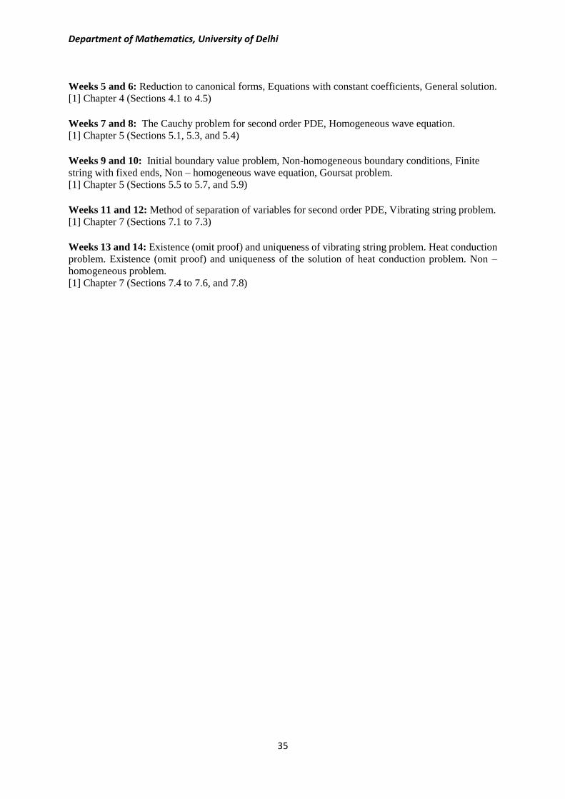
Weeks 5 and 6: Reduction to canonical forms, Equations with constant coefficients, General solution.
[1] Chapter 4 (Sections 4.1 to 4.5)
Weeks 7 and 8: The Cauchy problem for second order PDE, Homogeneous wave equation. [1] Chapter 5 (Sections 5.1, 5.3, and 5.4)
Weeks 9 and 10: Initial boundary value problem, Non-homogeneous boundary conditions, Finite
string with fixed ends, Non – homogeneous wave equation, Goursat problem.
[1] Chapter 5 (Sections 5.5 to 5.7, and 5.9)
Weeks 11 and 12: Method of separation of variables for second order PDE, Vibrating string problem.
[1] Chapter 7 (Sections 7.1 to 7.3)
Weeks 13 and 14: Existence (omit proof) and uniqueness of vibrating string problem. Heat conduction
problem. Existence (omit proof) and uniqueness of the solution of heat conduction problem. Non –
homogeneous problem. [1] Chapter 7 (Sections 7.4 to 7.6, and 7.8)

Department of Mathematics, University of Delhi
36
BMH409: Riemann Integration & Series of Functions
Total Marks: 100 (Theory: 75 and Internal Assessment: 25)
Workload: 5 Lectures (per week), 1 Tutorial (per week per student)
Duration: 14 Weeks (70 Hrs.) Examination: 3 Hrs.
Course Objectives: To understand the integration of bounded functions on a closed and
bounded interval and its extension to the cases where either the interval of integration is infinite,
or the integrand has infinite limits at a finite number of points on the interval of integration.
The sequence and series of real valued functions, and an important class of series of functions
(i.e., power series).
Course Learning Outcomes: The course will enable the students to learn about:
i) Some of the families and properties of Riemann integrable functions, and the
applications of the fundamental theorems of integration.
ii) Beta and Gamma functions and their properties.
iii) The valid situations for the inter-changeability of differentiability and integrability with
infinite sum, and approximation of transcendental functions in terms of power series.
Course Contents:
Unit 1: Riemann Integration (Lectures: 25)
Definition of Riemann integration, Inequalities for upper and lower Darboux sums, Necessary
and sufficient conditions for the Riemann integrability, Definition of Riemann integration by
Riemann sum and equivalence of the two definitions, Riemann integrability of monotone
functions and continuous functions, Properties of Riemann integrable functions, Definitions of
piecewise continuous and piecewise monotone functions and their Riemann integrability,
intermediate value theorem for integrals, Fundamental theorems (I and II) of calculus, and the
integration by parts.
Unit 2: Improper Integral (Lectures: 10)
Improper integrals of Type-I, Type-II and mixed type, Convergence of Beta and Gamma
functions, and their properties.
Unit 3: Sequence and Series of Functions (Lectures: 25)
Pointwise and uniform convergence of sequence of functions, Theorem on the continuity of
the limit function of a sequence of functions, Theorems on the interchange of the limit and
derivative, and the interchange of the limit and integrability of a sequence of functions.
Pointwise and uniform convergence of series of functions, Theorems on the continuity,
Derivability and integrability of the sum function of a series of functions, Cauchy criterion and
the Weierstrass M-Test for uniform convergence.
Unit 4: Power Series (Lectures: 10)
Definition of a power series, Radius of convergence, Absolute convergence (Cauchy-
Hadamard theorem), Uniform convergence, Differentiation and integration of power series,
Abel's Theorem.

Department of Mathematics, University of Delhi
37
References:
1. Bartle, Robert G., & Sherbert, Donald R. (2015). Introduction to Real Analysis (4th
ed.). Wiley India Edition. Delhi.
2. Denlinger, Charles G. (2011). Elements of Real Analysis. Jones and Bartlett (Student
Edition). First Indian Edition. Reprinted 2015.
3. Ghorpade, Sudhir R. & Limaye, B. V. (2006). A Course in Calculus and Real Analysis.
Undergraduate Texts in Mathematics, Springer (SIE). First Indian reprint.
4. Ross, Kenneth A. (2013). Elementary Analysis: The Theory of Calculus (2nd ed.).
Undergraduate Texts in Mathematics, Springer.
Teaching Plan (BMH409: Riemann Integration & Series of Functions): Week 1: Definition of Riemann integration, Inequalities for upper and lower Darboux sums.
[4] Chapter 6 [Section 32 (32.1 to 32.4)]
Week 2: Necessary and sufficient conditions for the Riemann integrability, Definition of Riemann
integration by Riemann sum and equivalence of the two definitions.
[4] Chapter 6 [Section 32 (32.5 to 32.10)]
Week 3: Riemann integrability of monotone functions and continuous functions, Algebra and
properties of Riemann integrable functions.
[4] Chapter 6 [Section 33 (33.1 to 33.6)]
Week 4: Definitions of piecewise continuous and piecewise monotone functions and their Riemann
integrability, Intermediate value theorem for integrals.
[4] Chapter 6 [Section 33 (33.7 to 33.10)]
Week 5: First and second fundamental theorems of integral calculus, and the integration by parts.
[4] Chapter 6 [Section 34 (34.1 to 34.3)]
Week 6: Improper integrals of Type-I, Type-II and mixed type.
[2] Chapter 7 [Section 7.8 (7.8.1 to 7.8.18)]
Week 7: Convergence of Beta and Gamma functions, and their properties.
[3] Pages 405 - 408
Week 8: Definitions and examples of pointwise and uniformly convergent sequence of functions.
[1] Chapter 8 [Section 8.1 (8.1.1 to 8.1.10)]
Week 9: Motivation for uniform convergence by giving examples. Theorem on the continuity of the
limit function of a sequence of functions.
[1] Chapter 8 [Section 8.2 (8.2.1 to 8.2.2)]
Week 10: The statement of the theorem on the interchange of the limit function and derivative, and its
illustration with the help of examples. The interchange of the limit function and integrability of a
sequence of functions.
[1] Chapter 8 [Section 8.2 (Theorems 8.2.3, and 8.2.4)]
Week 11: Pointwise and uniform convergence of series of functions, Theorems on the continuity,
derivability and integrability of the sum function of a series of functions.
[1] Chapter 9 [Section 9.4 (9.4.1 to 9.4.4)]

Department of Mathematics, University of Delhi
38
Week 12: Cauchy criterion for the uniform convergence of series of functions, and the Weierstrass M-
Test for uniform convergence.
[2] Chapter 9 [Section 9.4 (9.4.5 to 9.4.6)]
Week 13: Definition of a power series, Radius of convergence, Absolute and uniform convergence of
a power series.
[4] Chapter 4 (Section 23)
Week 14: Differentiation and integration of power series, Statement of Abel's Theorem and its
illustration with the help of examples.
[4] Chapter 4 [Section 26 (26.1 to 26.6)]

Department of Mathematics, University of Delhi
39
BMH410: Ring Theory & Linear Algebra-I
Total Marks: 100 (Theory: 75 and Internal Assessment: 25)
Workload: 5 Lectures (per week), 1 Tutorial (per week per student)
Duration: 14 Weeks (70 Hrs.) Examination: 3 Hrs.
Course Objectives: The objective of this course is to introduce the fundamental theory of two
objects, namely - rings and vector spaces, and their corresponding homomorphisms.
Course Learning Outcomes: The course will enable the students to learn about:
i) The fundamental concept of Rings, Fields, subrings, integral domains and the
corresponding morphisms.
ii) The concept of linear independence of vectors over a field, the idea of a finite
dimensional vector space, basis of a vector space and the dimension of a vector space.
iii) Basic concepts of linear transformations, the Rank-Nullity Theorem, matrix of a linear
transformation, algebra of transformations and the change of basis.
Course Contents:
Unit 1: Introduction of Rings (Lectures: 20)
Definition and examples of rings, Properties of rings, Subrings, Integral domains and fields,
characteristic of a ring. Ideals, Ideal generated by a subset of a ring, Factor rings, Operations
on ideals, Prime and maximal ideals.
Unit 2: Ring Homomorphisms (Lectures: 10)
Ring homomorphisms, Properties of ring homomorphisms, First, Second and Third
Isomorphism theorems for rings, The Field of quotients.
Unit 3: Introduction of Vector Spaces (Lectures: 20)
Vector spaces, Subspaces, Algebra of subspaces, Quotient spaces, Linear combination of
vectors, Linear span, Linear independence, Basis and dimension, Dimension of subspaces.
Unit 4: Linear Transformations (Lectures: 20)
Linear transformations, Null space, Range, Rank and nullity of a linear transformation, Matrix
representation of a linear transformation, Algebra of linear transformations. Isomorphisms,
Isomorphism theorems, Invertibility and the change of coordinate matrix.
References:
1. Gallian, Joseph. A. (2013). Contemporary Abstract Algebra (8th ed.). Cengage
Learning India Private Limited. Delhi. Fourth impression, 2015.
2. Friedberg, Stephen H., Insel, Arnold J., & Spence, Lawrence E. (2003). Linear
Algebra (4th ed.). Prentice-Hall of India Pvt. Ltd. New Delhi.

Department of Mathematics, University of Delhi
40
Teaching Plan (BMH410: Ring Theory & Linear Algebra-I):
Week 1: Definition and examples of rings, Properties of rings, Subrings. [1] Chapter 12
Week 2: Integral domains and fields, Characteristic of a ring.
[1] Chapter 13
Week 3 and 4: Ideals, Ideal generated by a subset of a ring, Factor rings, Operations on ideals, Prime
and maximal ideals.
[1] Chapter 14
Week 5: Ring homomorphisms, Properties of ring homomorphisms.
[1] Chapter 15 (up to Theorem 15.2)
Week 6: First, Second and Third Isomorphism theorems for rings, The Field of quotients.
[1] Chapter 15 (Theorems 15.3 to 15.6, Examples 10 to 12), and Exercises 3 and 4 on page 347.
Week 7: Vector spaces, subspaces, Algebra of subspaces.
[2] Chapter 1 (Sections 1.2, and 1.3)
Week 8: Linear combination of vectors, Linear span, Linear independence.
[2] Chapter 1 (Sections 1.4, and 1.5)
Weeks 9 and 10: Bases and dimension. Dimension of subspaces.
[2] Chapter 1 (Section 1.6)
Week 11: Linear transformations, Null space, Range, Rank and nullity of a linear transformation.
[2] Chapter 2 (Section 2.1)
Weeks 12 and 13: Matrix representation of a linear transformation, Algebra of linear transformations.
[2] Chapter 2 (Sections 2.2, and 2.3)
Week 14: Isomorphisms, Isomorphism theorems, Invertibility and the change of coordinate matrix.
[2] Chapter 2 (Sections 2.4, and 2.5)

Department of Mathematics, University of Delhi
41
Skill Enhancement Paper
SEC-2: Computer Algebra Systems and Related Software
Total Marks: 100 (Theory: 38, Internal Assessment: 12 and Practical: 50)
Workload: 2 Lectures (per week), 4 Practicals (per week per student)
Duration: 14 Weeks (28 Hrs. Theory + 56 Hrs. Practical) Examination: 2 Hrs.
Course Objectives: This course aims at familiarizing students with the usage of computer
algebra systems (/Mathematica/MATLAB/Maxima/Maple) and the statistical software R. The
basic emphasis is on plotting and working with matrices using CAS. Data entry and summary
commands will be studied in R. Graphical representation of data shall also be explored.
Course Learning Outcomes: This course will enable the students to:
i) Use CAS as a calculator, for plotting functions, animations and various applications of
matrices.
ii) Understand the use of the software R for entry, summary calculation, pictorial
representation of data and exploring relationship between data.
iii) Analyze, test, and interpret technical arguments on the basis of geometry.
Course Contents:
Unit 1: Introduction to CAS and Applications (Lectures: 10)
Computer Algebra System (CAS), Use of a CAS as a calculator, Computing and plotting
functions in 2D, Plotting functions of two variables using Plot3D and ContourPlot, Plotting
parametric curves surfaces, Customizing plots, Animating plots, Producing tables of values,
working with piecewise defined functions, Combining graphics.
Unit 2: Working with Matrices (Lectures: 6)
Simple programming in a CAS, Working with matrices, Performing Gauss elimination,
operations (transpose, determinant, inverse), Minors and cofactors, Working with large
matrices, Solving system of linear equations, Rank and nullity of a matrix, Eigenvalue,
eigenvector and diagonalization.
Unit 3: R - The Statistical Programming Language (Lectures: 6)
R as a calculator, Explore data and relationships in R. Reading and getting data into R:
Combine and scan commands, Types and structure of data items with their properties.
Manipulating vectors, Data frames, Matrices and lists. Viewing objects within objects.
Constructing data objects and conversions.
Unit 4: Data Analysis with R (Lectures: 6)
Summary commands: Summary statistics for vectors, Data frames, Matrices and lists.
Summary tables. Stem and leaf plot, Histograms. Plotting in R: Box-whisker plots, Scatter
plots, Pairs plots, Line charts, Pie charts, Cleveland dot charts and bar charts. Copy and save
graphics to other applications.
References:
1. Bindner, Donald & Erickson, Martin. (2011). A Student’s Guide to the Study, Practice,
and Tools of Modern Mathematics. CRC Press, Taylor & Francis Group, LLC.

Department of Mathematics, University of Delhi
42
2. Torrence, Bruce F., & Torrence, Eve A. (2009). The Student’s Introduction to
Mathematica®: A Handbook for Precalculus, Calculus, and Linear Algebra (2nd ed.).
Cambridge University Press.
3. Gardener, M. (2012). Beginning R: The Statistical Programming Language, Wiley.
Note: Theoretical and Practical demonstration should be carried out only in one of the CAS:
Mathematica/MATLAB/Maxima/Scilab or any other.
Practical/Lab work to be performed in Computer Lab.
Practicals:
[1] Chapter 12 (Exercises 1 to 4 and 8 to 12), Chapter 14 (Exercises 1 to 3)
[2] Chapter 3 [Exercises 3.2 (1 and 2), 3.3 (1, 2 and 4), 3.4 (1 and 2), 3.5 (1 to 4), 3.6 (2 and 3)].
[2] Chapter 6 (Exercises 6.2 and 6.3).
[2] Chapter 7 [Exercises 7.1 (1), 7.2, 7.3 (2), 7.4 (1) and 7.6].
Note: Relevant exercises of [3] Chapters 2 to 5 and 7 (The practical may be done on the database
to be downloaded from http://data.gov.in/).
Teaching Plan (Theory of SEC-1: Computer Algebra Systems and Related Software):
Weeks 1 to 3: Computer Algebra System (CAS), Use of a CAS as a calculator, Computing and plotting
functions in 2D, producing tables of values, working with piecewise defined functions, Combining
graphics. Simple programming in a CAS.
[1] Chapter 12 (Sections 12.1 to 12.5)
[2] Chapter 1, and Chapter 3 (Sections 3.1 to 3.6, and 3.8)
Weeks 4 and 5: Plotting functions of two variables using Plot3D and ContourPlot, Plotting parametric
curves surfaces, Customizing plots, Animating plots.
[2] Chapter 6 (Sections 6.2, and 6.3)
Weeks 6 to 8: Working with matrices, Performing Gauss elimination, operations (Transpose,
Determinant, Inverse), Minors and cofactors, working with large matrices, Solving system of linear
equations, Rank and nullity of a matrix, Eigenvalue, Eigenvector and diagonalization.
[2] Chapter 7 (Sections 7.1 to 7.8)
Weeks 9 to 11: R as a calculator, explore data and relationships in R. Reading and getting data into R:
Combine and scan commands, Types and structure of data items with their properties. Manipulating
vectors, Data frames, Matrices and Lists. Viewing objects within objects. Constructing data objects and
conversions.
[1] Chapter 14 (Sections 14.1 to 14.4)
[3] Chapter 2, and Chapter 3
Weeks 12 to 14: Summary commands: Summary statistics for vectors, Data frames, Matrices and lists.
Summary tables. Stem and leaf plot, histograms. Plotting in R: Box-whisker plots, Scatter plots, Pairs
plots, Line charts, Pie charts, Cleveland dot charts and Bar charts. Copy and save graphics to other
applications.
[1] Chapter 14 (Section 14.7)
[3] Chapter 5 (up to page 157), and Chapter 7.

Department of Mathematics, University of Delhi
43
Semester V
BMH511: Metric Spaces
Total Marks: 100 (Theory: 75, Internal Assessment: 25)
Workload: 5 Lectures (per week), 1 Tutorial (per week per student)
Duration: 14 Weeks (70 Hrs.) Examination: 3 Hrs,
Course Objectives: The course aims at providing the basic knowledge pertaining to metric
spaces such as open and closed balls, neighborhood, interior, closure, subspace, continuity,
compactness, connectedness etc.
Course Learning Outcomes: The course will enable the students to:
i) Understand the basic concepts of metric spaces;
ii) Correlate these concepts to their counter parts in real analysis;
iii) Appreciate the abstractness of the concepts such as open balls, closed balls,
compactness, connectedness etc. beyond their geometrical imaginations.
Course Contents:
Unit 1: Basic Concepts (Lectures: 15)
Metric spaces: Definition and examples, Sequences in metric spaces, Cauchy sequences,
Complete metric space.
Unit 2: Topology of Metric Spaces (Lectures: 25)
Open and closed ball, Neighborhood, Open set, Interior of a set, limit point of a set, derived
set, closed set, closure of a set, diameter of a set, Cantor’s theorem, Subspaces, Dense set.
Unit 3: Continuity & Uniform Continuity in Metric Spaces (Lectures: 15)
Continuous mappings, Sequential criterion and other characterizations of continuity, Uniform
continuity, Homeomorphism, Contraction mapping, Banach fixed point theorem.
Unit 4: Connectedness and Compactness (Lectures: 15)
Connectedness, Connected subsets of , Connectedness and continuous mappings,
Compactness, Compactness and boundedness, Continuous functions on compact spaces.
Reference:
1. Shirali, Satish & Vasudeva, H. L. (2009). Metric Spaces, Springer, First Indian Print.
Additional Readings:
1. Kumaresan, S. (2014). Topology of Metric Spaces (2nd ed.). Narosa Publishing House.
New Delhi.
2. Simmons, G. F. (2004). Introduction to Topology and Modern Analysis.
Tata McGraw Hill. New Delhi.

Department of Mathematics, University of Delhi
44
Teaching Plan (BMH511: Metric Spaces):
Week 1: Definition of metric space, Illustration using the usual metric on , Euclidean and max metric
on 2 , Euclidean and max metric on ,n
Discrete metric, Sup metric on B(S) and C[a, b], Integral
metric on C[a, b] etc.
[1] Chapter 1 [Section 1.2 (1.2.1, 1.2.2 ((i), (ii), (iv), (v), (viii), (ix), (x)), 1.2.3, and 1.2.4 (i))]
Week 2: Sequences in metric space, Definition of limit of a sequence, Illustration through examples,
Cauchy sequences.
[1] Chapter 1 [Section 1.3 (1.3.1, 1.3.2, 1.3.3 ((i), (iv)), 1.3.5), Section 1.4 (1.4.1 to 1.4.4)]
Week 3: Definition of complete metric spaces, Illustration through examples.
[1] Chapter 1 [Section 1.4 (1.4.5 to 1.4.7, 1.4.12 to 1.4.14(ii))]
Week 4: Open and closed balls, Neighborhood, Open sets, Examples and basic results.
[1] Chapter 2 [Section 2.1 (2.1.1 to 2.1.11 (except 2.1.6(ii)))]
Week 5: Interior point, Interior of a set, Limit point, Derived set, Examples and basic results.
[1] Chapter 2 [Section 2.1 (2.1.12 to 2.1.20)]
Week 6: Closed set, Closure of a set, Examples and basic results.
[1] Chapter 2 [Section 2.1 (2.1.21 to 2.1.35)]
Week 7: Bounded set, Diameter of a set, Cantor’s theorem.
[1] Chapter 2 [Section 2.1 (2.1.41 to 2.1.44)]
Week 8: Relativisation and subspaces, Dense sets.
[1] Chapter 2 [Section 2.2 (2.2.1 to 2.2.6), Section 2.3 (2.3.12 to 2.3.13(iv))]
Weeks 9 to 11: Continuous mappings, Sequential and other characterizations of continuity, Uniform
continuity, Homeomorphism, Contraction mappings, Banach fixed point theorem.
[1] Chapter 3 [Section 3.1, Section 3.4 (3.4.1 to 3.4.8), Section 3.5 (3.5.1 to 3.5.7(iii)), and Section 3.7
(3.7.1 to 3.7.5)]
Weeks 12 to 14: Connectedness and compactness, Definitions and properties of connected and compact
spaces.
[1] Chapter 4 [Section 4.1 (4.1.1 to 4.1.12)], and Chapter 5 [Section 5.1 (5.1.1 to 5.1.6), and Section 5.3
(5.3.1 to 5.3.10)]

Department of Mathematics, University of Delhi
45
BMH512: Group Theory-II
Total Marks: 100 (Theory: 75, Internal Assessment: 25)
Workload: 5 Lectures (per week), 1 Tutorial (per week per student)
Duration: 14 Weeks (70 Hrs.) Examination: 3 Hrs.
Course Objectives: The course will develop an in-depth understanding of one of the most
important branch of the abstract algebra with applications to practical real-world problems.
Classification of all finite Abelian groups (up to isomorphism) can be done.
Course Learning Outcomes: The course shall enable students to learn about:
i) Automorphisms for constructing new groups from the given group.
ii) External direct product 2 2Z Z applies to data security and electric circuits.
iii) Group actions, Sylow theorems and their applications to check nonsimplicity.
Course Contents:
Unit 1: Automorphisms and Properties (Lectures: 10)
Automorphism, inner automorphism, Automorphism groups, Automorphism groups of
finite and infinite cyclic groups, Characteristic subgroups, Commutator subgroup and its
properties; Applications of factor groups to automorphism groups.
Unit 2: External and Internal Direct Products of Groups (Lectures: 15)
External direct products of groups and its properties, The group of units modulo n as an external
direct product, Applications to data security and electric circuits; Internal direct products,
Classification of groups of order 2 ,p where p is a prime; Fundamental theorem of finite Abelian
groups and its isomorphism classes.
Unit 3: Group Action (Lectures: 20)
Group actions and permutation representations; Stabilizers and kernels of group actions;
Groups acting on themselves by left multiplication and consequences; Conjugacy in .nS
Unit 4: Sylow Theorems and Applications (Lectures: 25)
Conjugacy classes, The class equation, p-groups, The Sylow theorems and consequences,
Applications of Sylow theorems; Finite simple groups, Nonsimplicity tests; Generalized
Cayley’s theorem, Index theorem, Embedding theorem and applications. Simplicity of 5.A
References:
1. Dummit, David S., & Foote, Richard M. (2016). Abstract Algebra (3rd ed.). Student
Edition. Wiley India.
2. Gallian, Joseph. A. (2013). Contemporary Abstract Algebra (8th ed.). Cengage
Learning India Private Limited. Delhi. Fourth impression, 2015.

Department of Mathematics, University of Delhi
46
Teaching Plan (BMH512: Group Theory-II):
Week 1: Automorphism, Inner automorphism, Automorphism groups, Automorphism groups of finite
and infinite cyclic groups.
[2] Chapter 6 (pages 135 to 138)
Week 2: Characteristic subgroups, Commutator subgroup and its properties; Applications of factor
groups to automorphism groups.
[2] Exercises 1 to 4 on page 181, and Exercises 62, 68 on page 204.
[2] Chapter 9 (Theorem 9.4 and Example 17)
Week 3: External direct products of groups and its properties, The group of units modulo n as an external
direct product, Applications to data security and electric circuits.
[2] Chapter 8
Week 4: Internal direct products, Classification of groups of order 2 ,p where p is a prime.
[2] Chapter 9 (Section on internal direct products, pages 195 to 200)
Week 5: Statement of the Fundamental theorem of finite Abelian groups, The isomorphism classes of
Abelian groups.
[2] Chapter 11
Weeks 6 and 7: Group actions and permutation representations; Stabilizers and kernels of group
actions.
[1] Chapter 1 (Section 1.7), Chapter 2 (Section 2.2), and Chapter 4 (Section 4.1, except cycle
decompositions)
Weeks 8 and 9: Groups acting on themselves by left multiplication and consequences;
Conjugacy in .nS
[1] Chapter 4 [Section 4.2, and Section 4.3 (Pages 125-126)]
Week 10: Conjugacy classes, The class equation, p-groups.
[2] Chapter 24 (Pages 409 to 411)
Weeks 11 and 12: State three Sylow theorems and give their applications.
[2] Chapter 24 (Pages 412 to 421)
Weeks 13 and 14: Finite simple groups, Nonsimplicity tests; Generalized Cayley’s theorem, Index
theorem, Embedding theorem and applications; Simplicity of 5.A
[2] Chapter 25

Department of Mathematics, University of Delhi
47
Discipline Specific Elective (DSE) Course -1 (including practicals)
Any one of the following (at least two shall be offered by the college):
DSE-1 (i): Numerical Analysis
DSE-1 (ii): Mathematical Modeling and Graph Theory
DSE-1 (iii): C++ Programming for Mathematics
DSE-1 (i): Numerical Analysis
Total Marks: 150 (Theory: 75 + Internal Assessment: 25 + Practical: 50)
Workload: 4 Lectures (per week), 4 Periods practical (per week per student)
Duration: 14 Weeks (56 Hrs. Theory + 56 Hrs. practical) Examination: 3 Hrs.
Course Objectives: To comprehend various computational techniques to find approximate
value for possible root(s) of non-algebraic equations, to find the approximate solutions of
system of linear equations and ordinary differential equations. Also, the use of Computer
Algebra System (CAS) by which the numerical problems can be solved both numerically and
analytically, and to enhance the problem solving skills.
Course Learning Outcomes: The course will enable the students to learn the following:
i) Some numerical methods to find the zeroes of nonlinear functions of a single variable
and solution of a system of linear equations, up to a certain given level of precision.
ii) Interpolation techniques to compute the values for a tabulated function at points not in
the table.
iii) Applications of numerical differentiation and integration to convert differential
equations into difference equations for numerical solutions.
Course Contents:
Unit 1: Methods for Solving Algebraic and Transcendental Equations (Lectures: 16)
Algorithms, Convergence, Bisection method, False position method, Fixed point iteration
method, Newton's method, Secant method
Unit 2: Techniques to Solve Linear Systems (Lectures: 12) Partial and scaled partial pivoting, LU decomposition and its applications, Iterative methods:
Gauss-Jacobi, Gauss-Seidel and SOR methods.
Unit 3: Interpolation (Lectures: 12)
Lagrange and Newton interpolation, Piecewise linear interpolation.
Unit 4: Numerical Differentiation and Integration (Lectures: 16)
First order and higher order approximation for first derivative, Approximation for second
derivative. Numerical integration by closed Newton-Cotes formula: trapezoidal rule, Simpson's
rule and its error analysis. Euler’s method to solve ODE’s.
Note: Emphasis is to be laid on the algorithms of the above numerical methods.

Department of Mathematics, University of Delhi
48
Reference:
1. Bradie, Brian. (2006). A Friendly Introduction to Numerical Analysis. Pearson
Education, India. Dorling Kindersley (India) Pvt. Ltd. Third impression 2011.
Additional Readings:
1. Jain, M. K., Iyengar, S. R. K., & Jain, R. K. (2012). Numerical Methods for Scientific
and Engineering Computation. (6th ed.). New Age International Publisher, India, 2016.
2. Gerald, C. F., & Wheatley, P. O. (2008). Applied Numerical Analysis (7th ed.). Pearson
Education. India.
Practical/Lab work to be performed in Computer Lab:
Use of computer algebra software (CAS), for example Mathematica/MATLAB/Maple/
Maxima/Scilab etc., for developing the following numerical programs:
(1) Bisection method
(2) Newton Raphson method
(3) Secant method
(4) Regula Falsi method
(5) LU decomposition method
(6) Gauss-Jacobi method
(7) SOR method
(8) Gauss-Seidel method
(9) Lagrange interpolation
(10) Newton interpolation
(11) Trapezoidal rule
(12) Simpson's rule
(13) Euler’s method
Note: For any of the CAS: Mathematica /MATLAB/ Maple/Maxima /Scilab etc., data types-
simple data types, floating data types, character data types, arithmetic operators and operator
precedence, variables and constant declarations, expressions, input/output, relational operators,
logical operators and logical expressions, control statements and loop statements, Arrays
should be introduced to the students.
Teaching Plan (Theory of DSE-l (i): Numerical Analysis):
Week 1: Algorithms, Convergence, Order of convergence and examples.
[1] Chapter 1 (Sections 1.1, and 1.2)
Week 2: Bisection method, False position method and their convergence analysis, Stopping condition
and algorithms.
[1] Chapter 2 (Sections 2.1, and 2.2)
Week 3: Fixed point iteration method, its order of convergence and stopping condition.
[1] Chapter 2 (Section 2.3)
Week 4: Newton's method, Secant method, their order of convergence and convergence analysis.
[1] Chapter 2 (Sections 2.4, and 2.5)

Department of Mathematics, University of Delhi
49
Week 5: Examples to understand partial and scaled partial pivoting. LU decomposition.
[1] Chapter 3 (Sections 3.2, and 3.5, up to Example 3.15)
Weeks 6 and 7: Application of LU decomposition to solve system of linear equations. Gauss-Jacobi
method, Gauss-Seidel and SOR iterative methods to solve system of linear equations.
[1] Chapter 3 (Sections 3.5, and 3.8)
Week 8: Lagrange interpolation: Linear and higher order interpolation, and error in it.
[1] Chapter 5 (Section 5.1)
Weeks 9 and 10: Divided difference and Newton interpolation. Piecewise linear interpolation.
[1] Chapter 5 (Sections 5.3, and 5.5)
Weeks 11 and 12: First order and higher order approximation for first derivative and error in the
approximation. Second order forward, Backward and central difference approximations for second
derivative.
[1] Chapter 6 (Section 6.2)
Week 13: Numerical integration: Trapezoidal rule, Simpson's rule and its error analysis.
[1] Chapter 6 (Section 6.4)
Week 14: Euler’s method to solve first order ODE initial value problems.
[1] Chapter 7 (Section 7.2 up to page 562)

Department of Mathematics, University of Delhi
50
DSE-1 (ii): Mathematical Modeling and Graph Theory
Total Marks: 150 (Theory: 75 + Internal Assessment: 25 + Practical: 50)
Workload: 4 Lectures (per week), 4 Periods practical (per week per student)
Duration: 14 Weeks (56 Hrs. Theory + 56 Hrs. practical) Examination: 3 Hrs.
Course Objectives: The main objective of this course is to teach students how to model
physical problems using differential equations and solve them. Also, the use of Computer
Algebra Systems (CAS) by which the listed problems can be solved both numerically and
analytically.
Course Learning Outcomes: The course will enable the students to learn the following:
i) The use of mathematics software to observe the implementations of the above
mentioned methods efficiently, and to enhance the problem solving skills.
ii) To solve physical problems using differential equations.
Course Contents:
Unit 1: Power Series Solutions (Lectures: 16)
Power series solution of a differential equation about an ordinary point, Solution about a
regular singular point, The method of Frobenius. Legendre’s and Bessel’s equation.
Unit 2: Laplace Transforms (Lectures: 8)
Laplace transform and inverse transform, application to initial value problem up to second order.
Unit 3: Monte Carlo Simulation (Lectures: 16)
Monte Carlo Simulation Modeling: Simulating deterministic behavior (area under a curve,
volume under a surface); Generating Random Numbers: Middle square method, Linear
congruence; Queuing Models: Harbor system, Morning rush hour. Overview of optimization
modeling; Linear Programming Model: Geometric solution, Algebraic solution, Simplex
method, Sensitivity analysis.
Unit 4: Graph Theory (Lectures: 16)
Graphs, Diagraphs, Networks and subgraphs, Vertex degree, Paths and cycles, Regular and
bipartite graphs, Four cube problem, Social networks, Exploring and traveling, Eulerian and
Hamiltonian graphs, Applications to dominoes, Diagram tracing puzzles, Knight’s tour
problem, Gray codes.
References:
1. Aldous, Joan M., & Wilson, Robin J. (2007). Graphs and Applications: An Introductory
Approach. Springer. Indian Reprint.
2. Edwards, C. Henry, Penney, David E., & Calvis, David T. (2015). Differential Equation
and Boundary Value Problems: Computing and Modeling (5th ed.). Pearson.
3. Giordano, Frank R., Fox, William P., & Horton, Steven B. (2014). A First Course in
Mathematical Modeling (5th ed.). Brooks/Cole, Cengage Learning.
Note: [ 1 ] Chapter 1 (Section 1.1), Chapter 2 (Sections 2.1 to 2.4), Chapter 3 (Sections 3.1 to
3.3) are to be reviewed only. This is in order to understand the models on Graph Theory.

Department of Mathematics, University of Delhi
51
Practical / Lab work to be performed in Computer Lab:
Modeling of the following problems using Mathematica/MATLAB/Maple /Maxima/Scilab etc.
(i). Plotting of Legendre polynomial for n = 1 to 5 in the interval [0, 1]. Verifying
graphically that all the roots of Pn (x) lie in the interval [0, 1].
(ii). Automatic computation of coefficients in the series solution near ordinary points.
(iii). Plotting of the Bessel’s function of first kind of order 0 to 3.
(iv). Automating the Frobenius Series Method.
(v). Random number generation and then use it for one of the following:
a) Simulate area under a curve.
b) Simulate volume under a surface.
(vi). Programming of either one of the queuing model:
a) Single server queue (e.g. Harbor system).
b) Multiple server queue (e.g. Rush hour).
(vii). Programming of the Simplex method for 2 / 3 variables.
Teaching Plan (Theory of DSE-l (ii): Mathematical Modeling and Graph Theory):
Weeks 1 and 3: Power series solution of a differential equation about an ordinary point, Solution about
a regular singular point. Legendre’s equation. The method of Frobenius.
[2] Chapter 8 (Sections 8.1 to 8.3)
Week 4: Bessel’s equation. Bessel’s function of first kind.
[2] Chapter 8 [Section 8.5 up to Equation (19), page 551)]
Weeks 5 and 6: Laplace transform and inverse transform, Application to initial value problem up to
second order.
[2] Chapter 7 (Sections 7.1 to 7.3)
Weeks 7 and 8: Monte Carlo Simulation Modeling: Simulating deterministic behavior (area under a
curve, volume under a surface), Generating Random Numbers: Middle square method, Linear
congruence. Queuing Models: Harbor system, Morning rush hour.
[3] Chapter 5 (Sections 5.1 to 5.2, and 5.5)
Weeks 9 and 10: Overview of optimization modeling, Linear Programming Model: Geometric
solution, Algebraic solution, Simplex method, Sensitivity analysis.
[3] Chapter 7
Weeks 11 and 12: Graphs, Diagraphs, Networks and subgraphs, Vertex degree, Paths and cycles,
Regular and bipartite graphs, Four cube problem, Social networks.
[1] Chapter 1 (Section 1.1), and Chapter 2
Weeks 13 and 14: Overview of optimization modeling, Linear Programming Model: Geometric
solution, Algebraic solution, Simplex method, Sensitivity analysis.
[1] Chapter 3

Department of Mathematics, University of Delhi
52
DSE-1 (iii): C++ Programming for Mathematics
Total Marks: 150 (Theory: 75 + Internal Assessment: 25 + Practical: 50)
Workload: 4 Lectures (per week), 4 Periods practical (per week per student)
Duration: 14 Weeks (56 Hrs. Theory + 56 Hrs. practical) Examination: 3 Hrs.
Course Objectives: This course introduces C++ programming in the idiom and context of
mathematics and imparts a starting orientation using available mathematical libraries, and their
applications.
Course Learning Outcomes: After completion of this paper, student will be able to:
i) Understand and apply the programming concepts of C++ which is important to
mathematical investigation and problem solving.
ii) Use mathematical libraries for computational objectives.
iii) Represent the outputs of programs visually in terms of well formatted text and plots.
Course Contents:
Unit 1: C++ Essentials (Lectures: 16)
Fundamentals of programming, Organization of logic flow in stored program model of
computation, C++ as a general purpose programming language, Structure of a C++ program,
Common compilers and IDE’s, Basic data-types, Variables and literals in C++, Operators,
Expressions, Evaluation precedence, and Type compatibility. Outline of program development
in C++, Debugging and testing.
Applications: Greatest common divisor, and Random number generation.
Unit 2: Working with Structured Data (Lectures: 12)
Structured data-types in C++, Arrays and manipulating data in arrays with applications in
factorization of an integer and finding Euler’s totient; Objects and classes: Information hiding,
Modularity, Constructors and Destructors, Methods and Polymorphism.
Applications: Cartesian geometry using points (2 & 3-dimensional), and Pythagorean triples.
Unit 3: Working with Containers and Templates (Lectures: 16)
Containers and Template Libraries: Sets, Iterators, Multisets, Vectors, Maps, Lists, Stacks and
Queues. Applications: Basic set algebra, Modulo arithmetic, Permutations, and Polynomials.
Unit 4: Using Mathematical Libraries and Packages (Lectures: 12)
Arbitrary precision arithmetic using the GMP package; Linear algebra: Two-dimensional
arrays in C++ with applications in finding Eigenvalues, Eigenvectors, Rank, Nullity, and
Solving system of linear equations in matrices. Features of C++ for input/output and
visualization: Strings, Streams, Formatting methods, Processing files in a batch, Command-
line arguments, Visualization packages and their use in plots.
Reference:
1. Scheinerman, Edward (2006). C++ for Mathematicians: An Introduction for Students
and Professionals. Chapman & Hall/CRC. Taylor & Francis Group, LLC.

Department of Mathematics, University of Delhi
53
Additional Readings:
1. Dale, Nell & Weems, Chip (2013). Programming and Problem Solving with C++ (6th
ed.). Comprehensive Edition. Jones & Bartlett Learning.
2. Gottschling, Peter (2016). Discovering Modern C++: An Intensive Course for
Scientists, Engineers, and Programmers. Addison-Wesley. Pearson Education, Inc.
3. Josuttis, Nicolai M. (2012). The C++ Standard Library: A Tutorial and Reference (2nd
ed.). Addison-Wesley. Pearson Education, Inc.
4. Lippman, Stanley B. (2000). Essential C++. Addison-Wesley.
5. Stroustrup, Bjarne (2013). The C++ Programming Language (4th ed.). Addison-Wesley.
Practical / Lab work to be performed in Computer Lab:
A: Preparatory (Practical Sessions: 8 Hrs.)
1. Setting up of C++ programming environment on Linux/Windows/Mac-OS;
gcc/g++/mingw/cc, Program-development methodology and use IDE’s or other tools.
2. Demonstration of sample programs for
a. “Hello World”
b. Sum of an arithmetic progression.
c. Value of sin x using series expansion.
3. Finding/demonstrating:
a. Machine epsilon.
b. Integer and float overflow/underflow.
c. Iteration and selection based logic.
(provide a list of 8-10 problems suitable to learners needs)
B: Evaluative:
Set-I: (Practical Sessions: 8 Hrs.)
1. Greatest common divisor (including Euclid’s Method).
2. Random number generation (including a Monte Carlo Program).
Set-II: (Practical Sessions: 12 Hrs.)
1. Factorization of an integer, and Euler’s totient.
2. Cartesian geometry using points (2 & 3-dimensional).
3. Pythagorean triples.
Set-III: (Practical Sessions: 16 Hrs.)
1. Basic set algebra.
2. Modulo arithmetic.
3. Permutations.
4. Polynomials.

Department of Mathematics, University of Delhi
54
Set-IV: (Practical Sessions: 12 Hrs.)
1. Arbitrary precision arithmetic using the GMP package.
2. Finding Eigenvalues, Eigenvectors, Rank, Nullity, and Solving system of linear
equations in matrices.
3. Plots (using the GNU plotutils package).
Note. Exception handling in lab-exercises (SET-I to IV), Comments/Documentation using
Doxygen may be emphasized.
Teaching Plan (Theory of DSE-1 (iii) C++ Programming for Mathematics):
Week 1: Fundamentals of programming, Organization of logic flow in stored program model of
computation, C++ as a general purpose programming language, Structure of a C++ program, Common
compilers and IDE’s, Basic data-types.
[1] Chapter 1, and Chapter 2 (Sections 2.1 to 2.3)
Week 2: Variables and literals in C++, Operators, Expressions, Evaluation precedence, and Type
compatibility. Outline of program development in C++, Debugging and testing.
[1] Chapter 2 (Sections 2.4 to 2.9)
Weeks 3 and 4: Applications: Greatest common divisor, and Random number generation.
[1] Chapter 3, and Chapter 4
Week 5: Structured data-types in C++, Arrays and manipulating data in arrays.
Applications: Factorization of an integer, and Euler’s totient.
[1] Chapter 5 (Sections 5.1 to 5.4)
Weeks 6 and 7: Objects and classes: Information hiding, Modularity, Constructors and Destructors,
Methods and Polymorphism. Applications: Cartesian geometry using points (two and three
dimensional), and Pythagorean triples.
[1] Chapter 6, and Chapter 7
Weeks 8 and 9: Containers and Template Libraries: Sets, Iterators, Multisets, Vectors, Maps, Lists,
Stacks and Queues with applications in basic set algebra.
[1] Chapter 8 [Sections 8.1 to 8.7 (8.7.1 – 8.7.3)]
Weeks 10 and 11: Applications: Modulo arithmetic, Permutations, and Polynomials.
[1] Chapter 9, Chapter 11 (Sections 11.1, and 11.2), and Chapter 12 (Sections 12.1 to 12.3)
Week 12: Arbitrary precision arithmetic using the GMP package; Linear algebra: Two-dimensional
arrays in C++ with applications in finding Eigenvalues, Eigenvectors, Rank, Nullity, and Solving
system of linear equations in matrices.
[1] Chapter 13 [Sections 13.1, and 13.2 (13.2.1, 13.2.2)]
Weeks 13 and 14: Features of C++ for input/output & visualization: Strings, Streams, Formatting
methods, Processing files in a batch, Command-line arguments, Visualization packages and their use in
plots.
[1] Chapter 14 [Sections 14.1 to 14.6, and 14.8 (14.8.1-14.8.3)]

Department of Mathematics, University of Delhi
55
Discipline Specific Elective (DSE) Course - 2
Any one of the following (at least two shall be offered by the college):
DSE-2 (i): Probability Theory and Statistics
DSE-2 (ii): Discrete Mathematics
DSE-2 (iii): Cryptography and Network Security
DSE-2 (i): Probability Theory and Statistics
Total Marks: 100 (Theory: 75 + Internal Assessment: 25)
Workload: 5 Lectures (per week), 1 Tutorial (per week per student)
Duration: 14 Weeks (70 Hrs.) Examination: 3 Hrs.
Course Objectives: To make the students familiar with the basic statistical concepts and tools
which are needed to study situations involving uncertainty or randomness. The course intends
to render the students to several examples and exercises that blend their everyday experiences
with their scientific interests.
Course Learning Outcomes: This course will enable the students to learn:
i) Distributions to study the joint behavior of two random variables.
ii) To establish a formulation helping to predict one variable in terms of the other, i.e.,
correlation and linear regression.
iii) Central limit theorem, which helps to understand the remarkable fact that: the empirical
frequencies of so many natural populations, exhibit a bell shaped curve.
Course Contents:
Unit 1: Probability Functions and Moment Generating Function (Lectures: 20)
Sample space, Probability set function, Real random variables - Discrete and continuous,
Cumulative distribution function, Probability mass/density functions, Transformations,
Mathematical expectation, Moments, Moment generating function, Characteristic function.
Unit 2: Univariate Discrete and Continuous Distributions (Lectures: 20)
Discrete distributions: Uniform, Bernoulli, Binomial, Negative binomial, Geometric and
Poisson; Continuous distributions: Uniform, Gamma, Exponential, Chi-square, Beta and
normal; Normal approximation to the binomial distribution.
Unit 3: Bivariate Distribution (Lectures: 10)
Joint cumulative distribution function and its properties, Joint probability density function,
Marginal distributions, Expectation of function of two random variables, Joint moment
generating function, Conditional distributions and expectations.
Unit 4: Correlation, Regression and Central Limit Theorem (Lectures: 20)
The Correlation coefficient, Covariance, Calculation of covariance from joint moment
generating function, Independent random variables, Linear regression for two variables, The
method of least squares, Bivariate normal distribution, Chebyshev’s theorem, Strong law of
large numbers, Central limit theorem and weak law of large numbers.

Department of Mathematics, University of Delhi
56
References:
1. Hogg, Robert V., McKean, Joseph W., & Craig, Allen T. (2013). Introduction to
Mathematical Statistics (7th ed.). Pearson Education, Inc.
2. Miller, Irwin & Miller, Marylees. (2014). John E. Freund’s Mathematical Statistics with
Applications (8th ed.). Pearson. Dorling Kindersley (India).
3. Ross, Sheldon M. (2014). Introduction to Probability Models (11th ed.). Elsevier Inc. AP.
Teaching Plan (DSE-2 (i): Probability Theory and Statistics):
Weeks 1 and 2: Sample space, Probability set function and examples, Random variable, Probability
mass/density function, Cumulative distribution function and its properties.
[1] Chapter 1 (Sections 1.1, 1.3, and 1.5)
Week 3: Discrete and continuous random variables, and Transformations.
[1] Chapter 1 (Sections 1.6, and 1.7)
Week 4: Expectation of random variables, and some special expectations: Mean, Variance, Standard
deviation, Moments and moment generating function, Characteristic function.
[1] Chapter 1 (Sections 1.8, and 1.9)
Week 5: The discrete distributions - Uniform, Bernoulli and binomial.
[2] Chapter 5 (Sections 5.2 to 5.4)
Week 6: The discrete distributions - negative Binomial, Geometric and Poisson.
[2] Chapter 5 (Sections 5.5, and 5.7)
Week 7: The continuous distributions - Uniform, Gamma, Exponential, Chi-square and Beta.
[2] Chapter 6 (Sections 6.2 to 6.4)
Week 8: Normal distribution, and normal approximation to the binomial distribution.
[2] Chapter 6 (Sections 6.5, and 6.6)
Weeks 9 and 10: Random vector: Discrete and continuous, Joint cumulative distribution function and
its properties, Joint probability mass/density function, Marginal probability mass function, and
expectation of two random variables, Joint moment generating function, Conditional distributions and
expectations.
[1] Chapter 2 (Sections 2.1, and 2.3)
Week 11: The Correlation coefficient, Covariance, Calculation of covariance from joint moment
generating function, Independent random variables.
[1] Chapter 2 (Section 2.4, and Section 2.5)
Week 12: Linear regression for two variables, and the method of least squares.
[2] Chapter 14 (Sections 14.1 to 14.3)
Week 13: Bivariate normal distribution; Chebyshev’s theorem.
[2] Chapter 6 (Section 6.7), and Chapter 4 (Section 4.4)
Week 14: Statement and interpretation of the strong law of large numbers, Central limit theorem and
the weak law of large numbers.
[3] Chapter 2 (Section 2.8, and Exercise 76, page 89)

Department of Mathematics, University of Delhi
57
DSE-2 (ii): Discrete Mathematics
Total Marks: 100 (Theory: 75 + Internal Assessment: 25)
Workload: 5 Lectures (per week), 1 Tutorial (per week per student)
Duration: 14 Weeks (70 Hrs.) Examination: 3 Hrs.
Course Objectives: This course aims at introducing the concepts of lattices, Boolean algebras,
switching circuits and graph theory. The course discusses some important applications of
Boolean algebra and graph theory in real life situations through switching circuits and shortest
path algorithms.
Course Learning outcomes: After the course, the student will be able to understand the
concepts of:
i) Lattices and their types;
ii) Boolean algebra, switching circuits and their applications;
iii) Graphs, their types and its applications in study of shortest path algorithms.
Course Contents:
Unit 1: Ordered Sets (Lectures: 10)
Definitions, Examples and basic properties of ordered sets, Order isomorphism, Hasse
diagrams, Dual of an ordered set, Duality principle, Maximal and minimal elements, Building
new ordered sets, Maps between ordered sets.
Unit 2: Lattices (Lectures: 20)
Lattices as ordered sets, Lattices as algebraic structures, Sublattices, Products and
homomorphisms; Definitions, Examples and properties of modular and distributive lattices,
The M3 – N5 Theorem with applications, Complemented lattice, Relatively complemented
lattice, Sectionally complemented lattice.
Unit 3: Boolean Algebras and Switching Circuits (Lectures: 20) Boolean Algebras, De Morgan’s laws, Boolean homomorphism, Representation theorem;
Boolean polynomials, Boolean polynomial functions, Disjunctive normal form and conjunctive
normal form, Minimal forms of Boolean polynomial, Quinn-McCluskey method, Karnaugh
diagrams, Switching circuits and applications of switching circuits.
Unit 4: Graph Theory (Lectures: 20) Introduction to graphs, Konigsberg Bridge problem, Instant insanity game; Definition,
examples and basic properties of graphs, Subgraphs, Pseudographs, Complete graphs, Bipartite
graphs, Isomorphism of graphs, Paths and circuits, Eulerian circuits, Hamiltonian cycles,
Adjacency matrix, Weighted graph, Travelling salesman problem, Shortest path, Dijkstra’s
algorithm.
References:
1. Davey, B. A., & Priestley, H. A. (2002). Introduction to lattices and order (2nd ed.).
Cambridge University press, Cambridge.

Department of Mathematics, University of Delhi
58
2. Goodaire, Edgar G., & Parmenter, Michael M. (2011). Discrete Mathematics with
graph theory (3rd ed.). Pearson Education (Singapore ) Pvt. Ltd. Indian Reprint.
3. Lidl, Rudolf & Pilz, Gunter. (2004). Applied Abstract Algebra (2nd ed.), Undergraduate
Texts in Mathematics. Springer (SIE). Indian Reprint.
4. Rosen, Kenneth H. (2012). Discrete Mathematics and its applications, with
combinatorics and graph theory. (7th ed.). McGraw Hill Education. Indian Reprint.
Teaching Plan (DSE-2 (ii): Discrete Mathematics):
Weeks 1 and 2: Definitions, Examples and basic properties of ordered sets, Order isomorphism, Hasse
diagrams, dual of an ordered set, Duality principle, Maximal and minimal elements, Building new
ordered sets, Maps between ordered sets.
[1] Chapter 1 (Sections 1.1 to 1.5 and 1.14 to 1.26, and 1.34 to 1.36)
[3] Chapter 1 [Section 1 (1.1 to 1.3)]
Weeks 3 and 4: Lattices as ordered sets, Lattices as algebraic structures, Sublattices, Products and
homomorphisms.
[1] Chapter 2 (Sections 2.1 to 2.19)
[3] Chapter 1 [Section 1 (1.5 to 1.20)]
Week 5: Definitions, Examples and properties of Modular and Distributive lattices.
[1] Chapter 4 (Sections 4.1 to 4.9)
[3] Chapter 1 [Section 2 (2.1 to 2.6).
Week 6: M3 – N5 Theorem with applications, Complemented lattice, Relatively complemented lattice,
sectionally complemented lattice.
[1] Chapter 4 (Sections 4.10, and 4.11)
[3] Chapter 1 [Section 2 (2.7 to 2.14)]
Weeks 7 and 8: Boolean Algebras, De Morgan’s laws, Boolean homomorphism, representation
theorem. Boolean polynomials, Boolean polynomial functions, Disjunctive normal form and
conjunctive normal form.
[3] Chapter 1 (Sections 3, and 4)
Week 9: Minimal forms of Boolean polynomial, Quinn-McCluskey method, Karnaugh diagrams.
[3] Chapter 1 (Section 6)
Week 10: Switching circuits and applications of switching circuits.
[3] Chapter 2 (Sections 7, and 8).
Weeks 11 and 12: Introduction to graphs, Konigsberg Bridge problem, Instant insanity game.
Definition, Examples and basic properties of graphs, Subgraphs, Pseudographs, Complete graphs,
Bipartite graphs, Isomorphism of graphs.
[2] Chapter 9 [Sections 9.1, 9.2 (9.2.1, 9.2.7), and 9.3]
Weeks 13 and 14: Paths and circuits, Eulerian circuits, Hamiltonian cycles, Adjacency matrix,
Weighted graph, Travelling salesman problem, shortest path, Dijkstra’s algorithm.
[2] Chapter 10 [Sections 10.1 to 10.4 (10.4.1 to 10.4.3)]

Department of Mathematics, University of Delhi
59
DSE-2 (iii): Cryptography and Network Security
Total Marks: 100 (Theory: 75 + Internal Assessment: 25)
Workload: 5 Lectures (per week), 1 Tutorial (per week per student)
Duration: 14 Weeks (70 Hrs.) Examination: 3 Hrs.
Course Objectives: This course helps the students to develop skills and knowledge of standard
concepts in cryptography and demonstrates how cryptography plays an important role in the
present digital world by knowing encryption and decryption techniques and secure data in
transit across data networks.
Course Learning Outcomes: After the course, the student will be able to:
i) Understand the fundamentals of Cryptography and Network Security, including data
and advanced encryption standard (DES & AES), RSA and elliptic curve cryptography.
ii) Encrypt and decrypt messages using block ciphers, sign and verify messages using well
known signature generation and verification algorithms.
iii) Acquire knowledge of standard algorithms that can be used to provide confidentiality,
integrity and authentication of data.
Course Contents:
Unit 1: Cryptography and Data Encryption Standard (DES) (Lectures: 20)
Overview of Cryptography, Computer security concepts, Security attacks, Symmetric cipher
model, Cryptanalysis and brute-force attack, Substitution techniques, Caesar cipher,
Monoalphabetic ciphers, Playfair cipher, Hill cipher, Polyalphabetic ciphers, One-time pad,
Transposition techniques, Binary and ASCII, Pseudo-random bit generation, Stream ciphers
and Block ciphers, The Feistal cipher, The data encryption standard (DES), DES example.
Unit 2: Algorithms and Advanced Encryption Standard (AES) (Lectures: 20)
Review of basic concepts in Number theory and Finite Fields: Divisibility, Polynomial and
modular arithmetic, Fermat’s and Euler’s theorems, The Chinese remainder theorem, Discrete
logarithm., Finite fields of the form GF(p) and GF(2n). Advanced encryption standard (AES),
AES transformation functions, AES key expansion, AES example.
Unit 3: Public-key Cryptography (Lectures: 15)
Principles of public-key cryptosystems, The RSA algorithm and security of RSA, Elliptic curve
arithmetic, Elliptic curve cryptography, Cryptographic Hash functions, Secure Hash algorithm.
Unit 4: Digital Signatures and Network Security (Lectures: 15)
Digital signatures, Elgamal and Schnorr digital signature schemes, Digital signature algorithm.
Wireless network and mobile device security, Email architecture, formats, threats and security,
Secure/Multipurpose Internet Mail Extension (S/MIME) and Pretty Good Privacy (PGP).
References:
1. Stallings, William (2017). Cryptography and Network Security, Principles and
Practice (7th ed.). Pearson Education Limited. England.

Department of Mathematics, University of Delhi
60
2. Trappe, Wade & Washington, Lawrence C. (2006). Introduction to Cryptography with
Coding Theory (2nd ed.). Pearson Education International.
Additional Reading:
1. Stinson, Douglas R. (2005). Cryptography Theory and Practice (3rd ed.). CRC Press.
Teaching Plan (DSE-2 (iii): Cryptography and Network Security):
Weeks 1 and 2: Overview of Cryptography, Computer security concepts, Security attacks, Symmetric
cipher model, Cryptanalysis and brute-force attack, Substitution techniques, Caesar cipher,
Monoalphabetic ciphers, Playfair cipher, Hill cipher, Polyalphabetic ciphers, One-time pad.
[2] Chapter 1
[1] Chapter 1 (Sections 1.1, and 1.3), Chapter 3 (Sections 3.1, 3.2)
Weeks 3 and 4: Transposition techniques, Binary and ASCII, Pseudo-random bit generation, Stream
ciphers and Block ciphers, The Feistal cipher, The Data Encryption Standard (DES), DES example.
[1] Chapter 3 (Section 3.3), and Chapter 4 (Sections 4.1 to 4.3)
[2] Chapter 2 (Sections 2.8, and 2.10)
Weeks 5 and 6: Review of basic concepts in Number theory and Finite Fields: Divisibility, Polynomial
and modular arithmetic, Statements of Fermat’s and Euler’s theorems, The Chinese remainder theorem,
Discrete logarithm, Finite fields of the form GF(p) and GF(2n).
[1] Chapter 1 (Sections 2.1 to 2.3, 2.5, 2.7, and 2.8), and Chapter 5 (Sections 5.4 to 5.6)
Weeks 7 and 8: Advanced encryption standard (AES), AES transformation functions, AES key
expansion, AES example.
[1] Chapter 6 [Sections 6.1 to 6.5 (up to page 195)]
Weeks 9 and 10: Principles of public-key cryptosystems, The RSA algorithm and security of RSA,
Elliptic curve arithmetic, Elliptic curve cryptography.
[1] Chapter 9 (Sections 9.1, and 9.2), and Chapter 10 (Sections 10.3, and 10.4)
Week 11: Cryptographic Hash functions, Secure Hash algorithm.
[1] Chapter 11 (Sections 11.1, and 11.5)
Weeks 12 and 13: Digital signatures, Elgamal and Schnorr digital signature schemes, The digital
signature algorithm. Wireless network and mobile device security.
[1] Chapter 13 (Sections 13.1 to 13.4), and Chapter 18 (Sections 18.1, and 18.2)
Week 14: Email architecture, threats and security, Secure/Multipurpose Internet Mail Extension
(S/MIME) and Pretty Good Privacy (PGP).
[1] Chapter 19 [Sections 19.1 to 19.5 (Confidentiality excluded)]

Department of Mathematics, University of Delhi
61
Semester VI
BMH613: Complex Analysis
Total Marks: 150 (Theory: 75, Internal Assessment: 25 and Practical: 50)
Workload: 4 Lectures (per week), 4 Practicals (per week per student)
Duration: 14 Weeks (56 Hrs. Theory + 56 Hrs. Practical) Examination: 3 Hrs.
Course Objectives: This course aims to introduce the basic ideas of analysis for complex
functions in complex variables with visualization through relevant practicals. Particular
emphasis has been laid on Cauchy’s theorems, series expansions and calculation of residues.
Course Learning Outcomes: The completion of the course will enable the students to:
i) Understand the significance of differentiability of complex functions leading to the
understanding of Cauchy-Riemann equations.
ii) Evaluate the contour integrals and understand the role of Cauchy-Goursat theorem and
the Cauchy integral formula.
iii) Expand some simple functions as their Taylor and Laurent series, classify the nature of
singularities, find residues and apply Cauchy Residue theorem to evaluate integrals.
Course Contents:
Unit 1: Analytic Functions and Cauchy-Riemann Equations (Lectures: 16)
Functions of complex variable, Mappings; Mappings by the exponential function, Limits,
Theorems on limits, Limits involving the point at infinity, Continuity, Derivatives,
Differentiation formulae, Cauchy-Riemann equations, Sufficient conditions for
differentiability; Analytic functions and their examples.
Unit 2: Elementary Functions and Integrals (Lectures: 14)
Exponential function, Logarithmic function, Branches and derivatives of logarithms,
Trigonometric function, Derivatives of functions, Definite integrals of functions, Contours,
Contour integrals and its examples, Upper bounds for moduli of contour integrals,
Unit 3: Cauchy’s Theorems and Fundamental Theorem of Algebra (Lectures: 12)
Antiderivatives, Proof of antiderivative theorem, Cauchy-Goursat theorem, Cauchy integral
formula; An extension of Cauchy integral formula, Consequences of Cauchy integral
formula, Liouville’s theorem and the fundamental theorem of algebra.
Unit 4: Series and Residues (Lectures: 14)
Convergence of sequences and series, Taylor series and its examples; Laurent series and its
examples, Absolute and uniform convergence of power series, Uniqueness of series
representations of power series, Isolated singular points, Residues, Cauchy’s residue theorem,
residue at infinity; Types of isolated singular points, Residues at poles and its examples.
Reference:
1. Brown, James Ward, & Churchill, Ruel V. (2014). Complex Variables and
Applications (9th ed.). McGraw-Hill Education. New York.

Department of Mathematics, University of Delhi
62
Additional Readings:
1. Bak, Joseph & Newman, Donald J. (2010). Complex analysis (3rd ed.). Undergraduate
Texts in Mathematics, Springer. New York.
2. Zills, Dennis G., & Shanahan, Patrick D. (2003). A First Course in Complex Analysis
with Applications. Jones & Bartlett Publishers, Inc.
3. Mathews, John H., & Howell, Rusell W. (2012). Complex Analysis for Mathematics
and Engineering (6th ed.). Jones & Bartlett Learning. Narosa, Delhi. Indian Edition.
(For practicals: Sample materials of files in the form Mathematica/Maple 2011.zip,
log to: www.jblearning.com/catalog/9781449604455/).
Practical / Lab work to be performed in Computer Lab:
Modeling of the following problems using Mathematica /Maple/MATLAB /Maxima/Scilab etc.
1. Make a geometric plot to show that the nth roots of unity are equally spaced points that
lie on the unit circle C1 (0) = {z: |z| = 1} and form the vertices of a regular polygon with
n sides, for n = 4, 5, 6, 7, 8.
2. Find all the solutions of the equation z3 = 8i and represent these geometrically.
3. Write parametric equations and make a parametric plot for an ellipse centered at the
origin with horizontal major axis of 4 units and vertical minor axis of 2 units.
Show the effect of rotation of this ellipse by an angle of 𝜋
6 radians and shifting of the
centre from (0,0) to (2,1), by making a parametric plot.
4. Show that the image of the open disk D1 (-1 - i ) = {z : |z + 1 + i | < 1} under the linear
transformation w = f(z) = (3 – 4i)z + 6 + 2i is the open disk:
D5 (-1 + 3i) = {w: |w + 1 – 3i| < 5}.
5. Show that the image of the right half plane Re z = x > 1 under the linear transformation
w = (-1 + i)z – 2 + 3i is the half plane 𝑣 > 𝑢 + 7, where u = Re(w), etc. Plot the map.
6. Show that the image of the right half plane A = {z : Re z 1
2 } under the mapping
1( )w f z
z is the closed disk 𝐷1(1)̅̅ ̅̅ ̅̅ ̅̅ = {w : |w - 1| ≤ 1} in the w- plane.
7. Make a plot of the vertical lines x = a, for a = -1, −1
2,
1
2, 1 and the horizontal lines
y = b, for b = -1, −1
2,
1
2, 1. Find the plot of this grid under the mapping
1( )w f z
z .
8. Find a parametrization of the polygonal path C = C1 + C2 + C3 from -1 + i to 3 - i, where
C1 is the line from: -1 + i to -1, C2 is the line from: -1 to 1 + i and C3 is the line from
1 + i to 3 - i. Make a plot of this path.

Department of Mathematics, University of Delhi
63
9. Plot the line segment ‘L’ joining the point A = 0 to B = 2 + i 𝜋
4 and give an exact
calculation of ∫ 𝑒𝑧𝑑𝑧1
𝐿.
10. Plot the semicircle ‘C’ with radius 1 centered at z = 2 and evaluate the contour integral
∫1
𝑧−2𝑑𝑧
1
𝐶.
11. Show that ∫ 𝑧𝑑𝑧1
𝐶1= ∫ 𝑧𝑑𝑧
1
𝐶2= 4 + 2𝑖 where C1 is the line segment from -1 - i to 3 + i
and C2 is the portion of the parabola x = y2 + 2y joining -1 - i to 3 + i. Make plots of
two contours C1 and C2 joining -1 - i to 3 + i .
12. Use ML inequality to show that 2
1 1
1 2 5C
dzz
, where C is the straight line
segment from 2 to 2 + i. While solving, represent the distance from the point z to the
points i and –i, respectively, i.e. |z – i| and |z + i| on the complex plane ₵.
13. Show that 1 22
C
dz
z , where z1/2 is the principal branch of the square root function and C
is the line segment joining 4 to 8 + 6i. Also plot the path of integration.
14. Find and plot three different Laurent series representations for the function
2
3( )
2f z
z z
, involving powers of z.
15. Locate the poles of 4 2
1( )
5 26 5f z
z z
and specify their order.
16. Locate the zeros and poles of 2
cot( )( )
zg z
z
and determine their order. Also justify
that Res(g, 0) = 2 3.
17. Evaluate
1 (0)
exp(2 )
C
z dz
, where 1 (0)C denotes the circle: {z: |z|=1} with positive
orientation. Similarly evaluate
3
4 3 2
(0)
1.
2C
dzz z z
Teaching Plan (Theory of BMH613: Complex Analysis):
Week 1: Functions of complex variable, Mappings, Mappings by the exponential function.
[1] Chapter 2 (Sections 12 to 14)
Week 2: Limits, Theorems on limits, Limits involving the point at infinity, Continuity.
[1] Chapter 2 (Sections 15 to 18)

Department of Mathematics, University of Delhi
64
Week 3: Derivatives, Differentiation formulae, Cauchy-Riemann equations, Sufficient conditions
for Differentiability.
[1] Chapter 2 (Sections 19 to 22)
Week 4: Analytic functions, Examples of analytic functions, Exponential function.
[1] Chapter 2 (Sections 24, and 25), and Chapter 3 (Section 29)
Week 5: Logarithmic function, Branches and Derivatives of Logarithms, Trigonometric functions.
[1] Chapter 3 (Sections 30, 31, and 34)
Week 6: Derivatives of functions, Definite integrals of functions, Contours.
[1] Chapter 4 (Sections 37 to 39)
Week 7: Contour integrals and its examples, upper bounds for moduli of contour integrals.
[1] Chapter 4 (Sections 40, 41, and 43).
Week 8: Antiderivatives, proof of antiderivative theorem.
[1] Chapter 4 (Sections 44, and 45)
Week 9: State Cauchy-Goursat theorem, Cauchy integral formula.
[1] Chapter 4 (Sections 46, and 50)
Week 10: An extension of Cauchy integral formula, Consequences of Cauchy integral formula,
Liouville’s theorem and the fundamental theorem of algebra.
[1] Chapter 4 (Sections 51 to 53)
Week 11: Convergence of sequences, Convergence of series, Taylor series, proof of Taylor’s theorem,
Examples.
[1] Chapter 5 (Sections 55 to 59)
Week 12: Laurent series and its examples, Absolute and uniform convergence of power series,
uniqueness of series representations of power series.
[1] Chapter 5 (Sections 60, 62, 63, and 66).
Week 13: Isolated singular points, Residues, Cauchy’s residue theorem, Residue at infinity. [1]:
Chapter 6 (Sections 68 to 71)
Week 14: Types of isolated singular points, Residues at poles and its examples.
[1] Chapter 6 (Sections 72 to 74)

Department of Mathematics, University of Delhi
65
BMH614: Ring Theory and Linear Algebra-II
Total Marks: 100 (Theory: 75, Internal Assessment: 25)
Workload: 5 Lectures (per week), 1 Tutorial (per week per student)
Duration: 14 Weeks (70 Hrs.) Examination: 3 Hrs.
Course Objectives: This course introduces the basic concepts of ring of polynomials and
irreducibility tests for polynomials over ring of integers, used in finite fields with applications
in Cryptography. This course emphasizes the application of techniques using the adjoint of a
linear operator and their properties to least squares approximation and minimal solutions to
systems of linear equations.
Courses Learning Outcomes: On completion of this course, the student will be able to:
i) Appreciate the significance of unique factorization in rings and integral domains.
ii) Compute with the characteristic polynomial, eigenvalues, eigenvectors, and
eigenspaces, as well as the geometric and the algebraic multiplicities of an eigenvalue
and apply the basic diagonalization result.
iii) Compute inner products and determine orthogonality on vector spaces, including
Gram-Schmidt orthogonalization to obtain orthonormal basis.
Course Contents:
Unit 1: Polynomial Rings and Unique Factorization Domain (UFD) (Lectures: 25)
Polynomial rings over commutative rings, Division algorithm and consequences, Principal
ideal domains, Factorization of polynomials, Reducibility tests, Irreducibility tests, Eisenstein
criterion, Unique factorization in Z[x]; Divisibility in integral domains, Irreducibles, Primes,
Unique factorization domains, Euclidean domains.
Unit 2: Dual Spaces and Diagonalizable Operators (Lectures: 15)
Dual spaces, Double dual, Dual basis, Transpose of a linear transformation and its matrix in
the dual basis, Annihilators; Eigenvalues, Eigenvectors, Eigenspaces and characteristic
polynomial of a linear operator; Diagonalizability, Invariant subspaces and Cayley-Hamilton
theorem; The minimal polynomial for a linear operator.
Unit 3: Inner Product Spaces (Lectures: 15)
Inner product spaces and norms, Orthonormal basis, Gram-Schmidt orthogonalization process,
Orthogonal complements, Bessel’s inequality.
Unit 4: Adjoint Operators and Their Properties (Lectures: 15)
The adjoint of a linear operator, Least squares approximation, Minimal solutions to systems of
linear equations, Normal, Self-adjoint, Unitary and orthogonal operators and their properties.
References:
1. Friedberg, Stephen H., Insel, Arnold J., & Spence, Lawrence E. (2003). Linear
Algebra (4th ed.). Prentice-Hall of India Pvt. Ltd. New Delhi.

Department of Mathematics, University of Delhi
66
2. Gallian, Joseph. A. (2013). Contemporary Abstract Algebra (8th ed.). Cengage
Learning India Private Limited. Delhi. Fourth impression, 2015.
Additional Readings:
1. Herstein, I. N. (2006). Topics in Algebra (2nd ed.). Wiley Student Edition. India.
2. Hoffman, Kenneth, & Kunze, Ray Alden (1978). Linear Algebra (2nd ed.). Prentice-
Hall of India Pvt. Limited. Delhi. Pearson Education India Reprint, 2015.
3. Lang, Serge (1987). Linear Algebra (3rd ed.). Springer.
Teaching Plan (BMH614: Ring Theory and Linear Algebra-II):
Week 1: Polynomial rings over commutative rings, Division algorithm and consequences, Principal
ideal domains.
[2] Chapter 16
Weeks 2 and 3: Factorization of polynomials, Reducibility tests, Irreducibility tests, Eisenstein’s
criterion, Unique factorization in Z[x].
[2] Chapter 17
Weeks 4 and 5: Divisibility in integral domains, Irreducibles, Primes, Unique factorization domains,
Euclidean domains.
[2] Chapter 18
Week 6: Dual spaces, Double dual, Dual basis, Transpose of a linear transformation and its matrix in
the dual basis, Annihilators.
[1] Chapter 2 (Section 2.6)
Weeks 7 and 8: Eigenvalues, Eigenvectors, Eigenspaces and characteristic polynomial of a linear
operator; Diagonalizability, Invariant subspaces and Cayley-Hamilton theorem; The minimal
polynomial for a linear operator.
[1] Chapter 5 (Sections 5.1, 5.2, and 5.4), and Chapter 7 (Section 7.3, Statement of Theorem 7.16)
Week 9: Inner product spaces and norms.
[1] Chapter 6 (Section 6.1)
Weeks 10 and 11: Orthonormal basis, Gram-Schmidt orthogonalization process, Orthogonal
complements, Bessel’s inequality.
[1] Chapter 6 (Section 6.2)
Week 12: The adjoint of a linear operator and its properties, Least squares approximation, Minimal
solutions to systems of linear equations.
[1] Chapter 6 (Section 6.3, Statement of Theorem 6.13 with applications)
Weeks 13 and 14: Normal, Self-adjoint, unitary and orthogonal operators and their properties.
[1] Chapter 6 (Sections 6.4, and 6.5, up to Theorem 6.21, page 385)

Department of Mathematics, University of Delhi
67
Discipline Specific Elective (DSE) Course - 3
Any one of the following (at least two shall be offered by the college):
DSE-3 (i): Mathematical Finance
DSE-3 (ii): Introduction to Information Theory and Coding
DSE-3 (iii): Biomathematics
DSE-3 (i): Mathematical Finance
Total Marks: 100 (Theory: 75 + Internal Assessment: 25)
Workload: 5 Lectures (per week), 1 Tutorial (per week per student)
Duration: 14 Weeks (70 Hrs.) Examination: 3 Hrs.
Course Objectives: This course is an introduction to the application of mathematics in
financial world, that enables the student to understand some computational and quantitative
techniques required for working in the financial markets and actuarial mathematics.
Course Learning outcomes: In this course, the student will learn the basics of:
i) Financial markets and derivatives including options and futures.
ii) Pricing and hedging of options, interest rate swaps and no-Arbitrage pricing concept.
iii) Stochastic analysis (Ito formula and Ito integration) and the Black-Scholes model.
Course Contents:
Unit 1: Interest Rates (Lectures: 20)
Interest rates, Types of rates, Measuring interest rates, Zero rates, Bond pricing, Forward rate,
Duration, Convexity, Exchange traded markets and OTC markets, Derivatives--Forward
contracts, Futures contract, Options, Types of traders, Hedging, Speculation, Arbitrage.
Unit 2: Mechanics and Properties of Options (Lectures: 15)
No Arbitrage principle, Short selling, Forward price for an investment asset, Types of Options,
Option positions, Underlying assets, Factors affecting option prices, Bounds on option prices,
Put-call parity, Early exercise, Effect of dividends.
Unit 3: Stochastic Analysis of Stock Prices and Black-Scholes Model (Lectures: 20) Binomial option pricing model, Risk neutral valuation (for European and American options on
assets following binomial tree model), Lognormal property of stock prices, Distribution of rate
of return, expected return, Volatility, estimating volatility from historical data, Extension of
risk neutral valuation to assets following GBM, Black-Scholes formula for European options.
Unit 4: Hedging Parameters, Trading Strategies and Swaps (Lectures: 15)
Hedging parameters (the Greeks: Delta, Gamma, Theta, Rho and Vega), Trading strategies
involving options, Swaps, Mechanics of interest rate swaps, Comparative advantage argument,
Valuation of interest rate swaps, Currency swaps, Valuation of currency swaps.

Department of Mathematics, University of Delhi
68
Reference:
1. Hull, J. C., & Basu, S. (2010). Options, Futures and Other Derivatives (7th ed.).
Pearson Education. New Delhi.
Additional Readings:
1. Luenberger, David G. (1998). Investment Science, Oxford University Press. Delhi.
2. Ross, Sheldon M. (2011). An elementary Introduction to Mathematical Finance
(3rd ed.). Cambridge University Press. USA.
Teaching Plan (DSE-3 (i): Mathematical Finance):
Weeks 1 and 2: Interest rates, Types of rates, measuring interest rates, zero rates, Bond pricing,
Forward rate, Duration, Convexity.
[1] Chapter 4 (Section 4.1 to 4.4, 4.6, 4.8, and 4.9)
Weeks 3 and 4: Exchange Traded Markets and OTC markets, Derivatives- Forward contracts, Futures
contract, Options, Types of traders, Hedging, Speculation, Arbitrage
[1] Chapter 1 (Sections 1.1 to 1.9)
Week 5: No Arbitrage principle, Short selling, Forward price for an investment asset.
[1] Chapter 5 (Sections 5.2 to 5.4)
Week 6: Types of Options, Option positions, Underlying assets, Factors affecting option prices.
[1] Chapter 8 (Sections 8.1 to 8.3), and Chapter 9 (Section 9.1)
Week 7: Bounds on option prices, Put-call parity, Early exercise, Effect of dividends.
[1] Chapter 9 (Sections 9.2 to 9.7)
Week 8: Binomial option pricing model, Risk neutral Valuation (for European and American options
on assets following binomial tree model).
[1] Chapter 11 (Sections 11.1 to 11.5)
Weeks 9 to 11: Lognormal property of stock prices, Distribution of rate of return, expected return,
Volatility, estimating volatility from historical data. Extension of risk neutral valuation to assets
following GBM (without proof), Black-Scholes formula for European options.
[1] Chapter 13 (Sections 13.1 to 13.4, 13.7, and 13.8)
Week 12: Hedging parameters (the Greeks: Delta, Gamma, Theta, Rho and Vega).
[1] Chapter 17 (Sections 17.1 to 17.9)
Week 13: Trading strategies Involving options.
[1] Chapter 10 (except box spreads, calendar spreads and diagonal spreads)
Week 14: Swaps, Mechanics of interest rate swaps, Comparative advantage argument, Valuation of
interest rate swaps, Currency swaps, Valuation of currency swaps
[1] Chapter 7 (Sections 7.1 to 7.4, and 7.7 to 7.9)

Department of Mathematics, University of Delhi
69
DSE-3(ii): Introduction to Information Theory and Coding
Total Marks: 100 (Theory: 75, Internal Assessment: 25)
Workload: 5 Lectures (per week), 1 Tutorial (per week per student)
Duration: 14 Weeks (70 Hrs.) Examination: 3 Hrs.
Course Objectives: This course aims to introduce the basic aspects of Information Theory and
Coding to the students. Shannon’s work form the underlying theme for the present course.
Construction of finite fields and bounds on the parameters of a linear code discussed.
Course Learning Outcomes: This course will enable the students to learn:
i) The output of the channel, a received signal is observed.
ii) The detection &correction of errors while transmission.
iii) Representation of a linear code by matrices and its encoding and decoding.
Course Contents:
Unit 1: Concepts of Information Theory (Lectures: 20) Communication processes, A model of communication system, A quantitative measure of
information, Binary unit of information, A measure of uncertainty, H function as a measure of
uncertainty, Sources and binary sources, Measure of information for two-dimensional discrete
finite probability schemes.
Unit 2: Entropy Function (Lectures: 20) A sketch of communication network, Entropy, Basic relationship among different entropies, A
measure of mutual information, Interpretation of Shannon’s fundamental inequalities; Redundancy,
Efficiency and channel capacity, Binary symmetric channel, Binary erasure channel, Uniqueness
of the entropy function, Joint entropy and conditional entropy, Relative entropy and mutual
information, Chain rules for entropy, Conditional relative entropy and conditional mutual
information, Jensen’s inequality and its characterizations, The log sum inequality and its
applications.
Unit 3: Concepts of Coding (Lectures: 15) Block codes, Hamming distance, Maximum likelihood decoding, Levels of error handling, Error
correction, Error detection, Erasure correction, Construction of finite fields, Linear codes, Matrix
representation of linear codes.
Unit 4: Bounds of Codes (Lectures: 15) Orthogonality relation, Encoding of linear codes, Decoding of linear codes, The singleton bound
and maximum distance separable codes, The sphere-packing bound and perfect codes, The Gilbert-
Varshamov bound, MacWilliams’ identities.
References:
1. Cover, Thomas M., & Thomas, Joy A. (2006). Elements of Information Theory (2nd
ed.). Wiley India. Indian Reprint 2014.
2. Gallian, Joseph. A. (2013). Contemporary Abstract Algebra(8th ed.).Cengage
Learning India Private Limited. Delhi. Fourth impression, 2015.
3. Reza, Fazlollah M. (1961). An Introduction to Information Theory. Dover Publications
Inc, New York. Reprint 1994.
4. Roth, Ron M. (2007). Introduction to Coding Theory. Cambridge University Press.

Department of Mathematics, University of Delhi
70
Teaching Plan (DSE-3(ii): Introduction to Information Theory and Coding):
Weeks 1 and 2: Communication processes, A model of communication system, A quantitative measure
of information, Binary unit of information.
[3] Chapter 1 (Sections 1.1 to 1.7)
Weeks 3 and 4: A measure of uncertainty, H function as a measure of uncertainty, Sources and binary
sources, Measure of information for two-dimensional discrete finite probability schemes.
[3] Chapter 3 (Sections 3.1 to 3.7)
Weeks 5 and 6: A sketch of communication network, Entropy, Basic relationship among different
entropies, A measure of mutual information, Interpretation of Shannon’s fundamental inequalities;
redundancy, efficiency and channel capacity, Binary symmetric channel, Binary erasure channel,
Uniqueness of the entropy function.
[3] Chapter 3 (Sections 3.9, 3.11 to 3.16, and 3.19)
[1] Chapter 2 (Section 2.1)
Weeks 7 and 8: Joint entropy and conditional entropy, Relative entropy and mutual information, Chain
rules for entropy, Conditional relative entropy and conditional mutual information, Jensen’s inequality
and its characterizations, The log sum inequality and its applications.
[1] Chapter 2 (Sections 2.2 to 2.7)
Weeks 9 and 10: Block codes, Hamming distance, Maximum likelihood decoding, Levels of error
handling, Error correction, Error detection, Erasure correction, Construction of finite fields.
[4] Chapter 1 (Sections 1.2 to 1.5, excluding 1.5.3), and Chapter 3 (Sections 3.1 to 3.4)
Weeks 11 and 12: Linear codes, Matrix representation of linear codes, Orthogonality relation,
Encoding of linear codes, Decoding of linear codes.
[4] Chapter 2 (Sections 2.1 to 2.4)
[2] Chapter 31 (Lemma and Theorem 31.3 on page 538)
Weeks 13 and 14: The singleton bound and maximum distance separable codes, The sphere-packing
bound and perfect codes, the Gilbert-Varshamov bound, MacWilliams’ identities.
[4] Chapter 4 (Sections 4.1 to 4.4), and Chapter 11 (Section 11.1)

Department of Mathematics, University of Delhi
71
DSE-3 (iii): Biomathematics
Total Marks: 100 (Theory: 75 + Internal Assessment: 25)
Workload: 5 Lectures (per week), 1 Tutorial (per week per student)
Duration: 14 Weeks (70 Hrs.) Examination: 3 Hrs.
Course Objectives: The focus of the course is on scientific study of normal functions in living
systems. The emphasis is on exposure to nonlinear differential equations with examples such
as heartbeat, chemical reactions and nerve impulse transmission. The basic concepts of the
probability to understand molecular evolution and genetics have also been applied.
Course Learning outcomes: Apropos conclusion of the course will empower the student to:
i) Learn the development, analysis and interpretation of bio mathematical models.
ii) Reinforce the skills in mathematical modeling.
iii) Appreciate the theory of bifurcation and chaos.
iv) Learn to apply the basic concepts of probability to molecular evolution and genetics.
Course Contents:
Unit 1: Modeling Biological Phenomenon (Lectures: 14)
Population growth, Administration of drugs, Cell division, Systems of linear ordinary
differential equations, Heartbeat, Nerve impulse transmission, Chemical reactions, Predator-
prey models.
Unit 2: Mathematics of Heart Physiology and Nerve Impulse Transmission (Lectures: 28)
Stability and oscillations: Epidemics, The phase plane and the Jacobian matrix, Local stability,
Stability, Limit cycles, Forced oscillations; Mathematics of Heart Physiology: The local model,
The Threshold effect, The phase plane analysis and the heartbeat model, A model of the cardiac
pacemaker; Mathematics of Nerve Impulse Transmission: Excitability and repetitive firing,
Travelling waves.
Unit 3: Bifurcation and Chaos (Lectures: 13)
Bifurcation, Bifurcation of a limit cycle, Discrete bifurcation and period-doubling, Chaos,
Stability of limit cycles, The Poincaré plane.
Unit 4: Modeling Molecular Evolution and Genetics (Lectures: 15)
Modelling Molecular Evolution: Matrix models of base substitutions for DNA sequences, The
Jukes-Cantor model, The Kimura models, Phylogenetic distances; Constructing Phylogenetic
Trees: Phylogenetic trees, Unweighted pair-group method with arithmetic means (UPGMA),
Neighbor joining method; Genetics: Mendelian genetics, Probability distributions in genetics.
References:
1. Allman, Elizabeth S., & Rhodes, John A. (2004). Mathematical Models in Biology:
An Introduction. Cambridge University Press.
2. Jones, D. S., Plank, M. J., & Sleeman, B. D. (2009). Differential Equations and
Mathematical Biology (2nd ed.). CRC Press, Taylor & Francis Group, LLC.

Department of Mathematics, University of Delhi
72
Additional Readings:
1. Murray, J. D. (2002). An Introduction to Mathematical Biology (3rd ed.). Springer.
2. Myint-U, Tyn (1977). Ordinary Differential Equation. Elsevier North-Holland, Inc.
3. Simmons, George F., & Krantz, Steven G. (2015). Differential Equations. McGraw-
Hill Education. Indian Reprint.
4. Strogatz, Steven H. (2009). Nonlinear Dynamics and Chaos (2nd ed.). Perseus Book
Publishing. LLC. Sarat Publication, Kolkata, India.
Teaching Plan (DSE-3 (iii): Biomathematics):
Week 1: Population growth, Administration of drugs, Cell division, Systems of linear ordinary
differential equations.
[2] Chapter 1 (Sections 1.1 to 1.3), and Chapter 3 (An overview of the methods in Sections 3.1 to 3.6)
Week 2: Heartbeat, Nerve impulse transmission
[2] Chapter 4 (Sections 4.2, and 4.3)
Week 3: Chemical reactions, Predator-prey models, Epidemics (Mathematical model).
[2] Chapter 4 (Sections 4.4, and 4.5), and Chapter 5 (Section 5.2)
Week 4: The phase plane and Jacobian matrix, Local stability.
[2] Chapter 5 (Sections 5.3, and 5.4)
Week 5: Stability, Limit cycles.
[2] Chapter 5 [Sections 5.5, and 5.6 (up to page number 137)]
Week 6: Limit cycle criterion and Poincaré-Bendixson Theorem (interpretation only, with Example
5.6.1), Forced oscillations.
[2] Chapter 5 [Section 5.6 (Page number 137 to 138), and Section 5.7)
Week 7: Mathematics of Heart Physiology: The local model, The Threshold effect, The phase plane
analysis and the heartbeat model.
[2] Chapter 6 (Sections 6.1 to 6.3)
Week 8: A model of the cardiac pacemaker, Excitability and repetitive firing.
[2] Chapter 6 (Section 6.5), and Chapter 7 (Section 7.1)
Week 9: Travelling waves, Bifurcation, Bifurcation of a limit cycle.
[2] Chapter 7 (Section 7.2), and Chapter 13 (Sections 13.1, and 13.2)
Weeks 10 and 11: Discrete bifurcation and period-doubling, Chaos, Stability of limit cycles, The
Poincaré plane.
[2] Chapter 13 (Sections 13.3 to 13.6)
Week 12: Matrix models of base substitutions for DNA sequences, The Jukes-Cantor model, The
Kimura models, Phylogenetic distances.
[1] Chapter 4 (Sections 4.4, and 4.5)
Week 13: Constructing Phylogenetic Trees: Phylogenetic trees, Unweighted pair-group method with
arithmetic means (UPGMA), Neighbor joining method.
[1] Chapter 5 (Sections 5.1 to 5.3)
Week 14: Genetics: Mendelian Genetics, Probability distributions in Genetics.
[1] Chapter 6 [Sections 6.1, and 6.2 (up to Equation 6.2 only)]

Department of Mathematics, University of Delhi
73
Discipline Specific Elective (DSE) Course - 4
Any one of the following (at least two shall be offered by the college):
DSE-4 (i): Number Theory
DSE-4 (ii): Linear Programming and Applications
DSE-4 (iii): Mechanics
DSE-4 (i): Number Theory
Total Marks: 100 (Theory: 75 and Internal Assessment: 25)
Workload: 5 Lectures (per week), 1 Tutorial (per week per student)
Duration: 14 Weeks (70 Hrs.) Examination: 3 Hrs.
Course Objectives: In number theory there are challenging open problems which are
comprehensible at undergraduate level, this course is intended to build a micro aptitude of
understanding aesthetic aspect of mathematical instructions and gear young minds to ponder
upon such problems. Also, another objective is to make the students familiar with simple
number theoretic techniques, to be used in data security.
Course Learning Outcomes: This course will enable the students to learn:
i) Some of the open problems related to prime numbers, viz., Goldbach conjecture etc.
ii) About number theoretic functions and modular arithmetic.
iii) Public crypto systems, in particular, RSA.
Course Contents:
Unit 1: Distribution of Primes and Theory of Congruencies (Lectures: 15)
Linear Diophantine equation, Prime counting function, Prime number theorem, Goldbach
conjecture, Fermat and Mersenne primes, Congruence relation and its properties, Linear
congruence and Chinese remainder theorem, Fermat's little theorem, Wilson's theorem.
Unit 2: Number Theoretic Functions (Lectures: 15) Number theoretic functions for sum and number of divisors, Multiplicative function, The
Mobius inversion formula, The greatest integer function. Euler’s phi-function and properties,
Euler’s theorem.
Unit 3: Primitive Roots (Lectures: 20)
The order of an integer modulo n, Primitive roots for primes, Composite numbers having
primitive roots; Definition of quadratic residue of an odd prime, and Euler’s criterion.
Unit 4: Quadratic Reciprocity Law and Public Key Encryption (Lectures: 20)
The Legendre symbol and its properties, Quadratic reciprocity, Quadratic congruencies with
composite moduli; Public key encryption, RSA encryption and decryption.

Department of Mathematics, University of Delhi
74
References:
1. Burton, David M. (2007). Elementary Number Theory (7th ed.). Tata Mc-Graw Hill
Edition, Indian Reprint.
2. Jones, G. A., &Jones, J. Mary. (2005). Elementary Number Theory. Undergraduate
Mathematics Series (SUMS). First Indian Print.
Additional Reading:
1. Neville Robinns. (2007). Beginning Number Theory (2nd ed.). Narosa Publishing
House Pvt. Limited, Delhi.
Teaching Plan (DSE-4 (i): Number Theory):
Week 1 : Linear Diophantine equation and its solutions, Distribution of primes, Prime counting
function, Statement of the prime number theorem, Goldbach conjecture.
[1] Chapter 2 (Section 2.5)
[2] Chapter 2 (Section 2.2)
Week 2: Fermat and Mersenne primes, Congruence relation and its basic properties, Linear congruence
equation and its solutions.
[2] Chapter 2 (Section 2.3)
[1] Chapter 4 (Sections 4.2, and 4.4)
Week 3: Chinese remainder theorem, to solve system of linear congruence for two variables, Fermat's
little theorem, Wilson's theorem.
[1] Chapter 4 (Section 4.4), Chapter 5 (Section 5.2 up to before pseudo-prime at page 90, Section 5.3)
Weeks 4 and 5: Number theoretic functions for sum and number of divisors, Multiplicative function,
and the Mobius inversion formula. The greatest integer function, Euler's phi-function.
[1] Chapter 6 (Sections 6.1 to 6.2), and Chapter 7 (Section 7.2)
Week 6: Euler's theorem, Properties of Euler’s phi-function.
[1] Chapter 7 (Sections 7.3, and 7.4)
Weeks 7 and 8: The order of an integer modulo n. Primitive roots for primes.
[1] Chapter 8 (Sections 8.1, and 8.2)
Week 9: Composite numbers having primitive roots.
[1] Chapter 8 (Section 8.3)
Week 10: Definition of quadratic residue of an odd prime, and Euler's criterion.
[1] Chapter 9 (Section 9.1)
Weeks 11 and 12: The Legendre symbol and its properties. Quadratic reciprocity law.
[1] Chapter 9 (Section 9.2 up to page 181, and Section 9.3)
Week 13: Quadratic congruencies with composite moduli.
[1] Chapter 9 (Section 9.4)
Week 14: Public key encryption, RSA encryption and decryption scheme.
[1] Chapter 10 (Section 10.1)
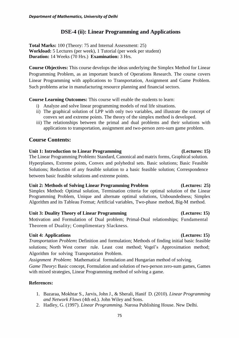
Department of Mathematics, University of Delhi
75
DSE-4 (ii): Linear Programming and Applications
Total Marks: 100 (Theory: 75 and Internal Assessment: 25)
Workload: 5 Lectures (per week), 1 Tutorial (per week per student)
Duration: 14 Weeks (70 Hrs.) Examination: 3 Hrs.
Course Objectives: This course develops the ideas underlying the Simplex Method for Linear
Programming Problem, as an important branch of Operations Research. The course covers
Linear Programming with applications to Transportation, Assignment and Game Problem.
Such problems arise in manufacturing resource planning and financial sectors.
Course Learning Outcomes: This course will enable the students to learn:
i) Analyze and solve linear programming models of real life situations.
ii) The graphical solution of LPP with only two variables, and illustrate the concept of
convex set and extreme points. The theory of the simplex method is developed.
iii) The relationships between the primal and dual problems and their solutions with
applications to transportation, assignment and two-person zero-sum game problem.
Course Contents:
Unit 1: Introduction to Linear Programming (Lectures: 15)
The Linear Programming Problem: Standard, Canonical and matrix forms, Graphical solution.
Hyperplanes, Extreme points, Convex and polyhedral sets. Basic solutions; Basic Feasible
Solutions; Reduction of any feasible solution to a basic feasible solution; Correspondence
between basic feasible solutions and extreme points.
Unit 2: Methods of Solving Linear Programming Problem (Lectures: 25)
Simplex Method: Optimal solution, Termination criteria for optimal solution of the Linear
Programming Problem, Unique and alternate optimal solutions, Unboundedness; Simplex
Algorithm and its Tableau Format; Artificial variables, Two-phase method, Big-M method.
Unit 3: Duality Theory of Linear Programming (Lectures: 15)
Motivation and Formulation of Dual problem; Primal-Dual relationships; Fundamental
Theorem of Duality; Complimentary Slackness.
Unit 4: Applications (Lectures: 15)
Transportation Problem: Definition and formulation; Methods of finding initial basic feasible
solutions; North West corner rule. Least cost method; Vogel’s Approximation method;
Algorithm for solving Transportation Problem.
Assignment Problem: Mathematical formulation and Hungarian method of solving.
Game Theory: Basic concept, Formulation and solution of two-person zero-sum games, Games
with mixed strategies, Linear Programming method of solving a game.
References:
1. Bazaraa, Mokhtar S., Jarvis, John J., & Sherali, Hanif D. (2010). Linear Programming
and Network Flows (4th ed.). John Wiley and Sons.
2. Hadley, G. (1997). Linear Programming. Narosa Publishing House. New Delhi.

Department of Mathematics, University of Delhi
76
3. Taha, Hamdy A. (2010). Operations Research: An Introduction (9th ed.). Pearson.
Additional Readings:
1. Hillier, F. S. & Lieberman, G. J. (2010). Introduction to Operations Research-
Concepts and Cases (9th ed.). Tata McGraw Hill.
2. Thie, Paul R., & Keough, G. E. (2014). An Introduction to Linear Programming and
Game Theory. (3rd ed.). Wiley India Pvt. Ltd.
Teaching Plan (DSE-4 (ii): Linear Programming and Applications):
Week 1 : The Linear Programming Problem: Standard, Canonical and matrix forms, Graphical solution.
[1] Chapter 1 (Section 1.1)
[2] Chapter 1 (Sections 1.1 to 1.4, and 1.6)
Weeks 2 and 3: Hyperplanes, Extreme points, Convex and polyhedral sets; Basic solutions. Basic
Feasible Solutions; Reduction of any feasible solution to a basic feasible solution; Correspondence
between basic feasible solutions and extreme points.
[2] Chapter 2 (Sections 2.16, 2.19, and 2.20), and Chapter 3 (Sections 3.4, and 3.10)
[1] Chapter 3 (Section 3.2)
Week 4: Simplex Method: Optimal solution, Termination criteria for optimal solution of the Linear
Programming Problem, Unique and alternate optimal solutions, Unboundedness.
[1] Chapter 3 (Sections 3.3, and 3.6)
Weeks 5 and 6: Simplex Algorithm and its Tableau Format.
[1] Chapter 3 (Sections 3.7, and 3.8).
Weeks 7 and 8: Artificial variables, Two-phase method, Big-M method.
[1] Chapter 4 (Sections 4.1 to 4.3)
Weeks 9 and 10: Motivation and Formulation of Dual problem; Primal-Dual relationships.
[1] Chapter 6 (Section 6.1, and 6.2, up to Example 6.4)
Week 11: Statements of the Fundamental Theorem of Duality and Complimentary Slackness
Theorem with examples.
[1] Chapter 6 (Section 6.2)
Weeks 12 and 13: Transportation Problem. Assignment problem.
[3] Chapter 5 (Sections 5.1, 5.3, and 5.4)
Week 14: Game Theory: Basic concept, Formulation and solution of two-person zero-sum games,
Games with mixed strategies, Linear Programming method of solving a game.
[2] Chapter 11 (Sections 11.12, and 11.13)

Department of Mathematics, University of Delhi
77
DSE-4 (iii): Mechanics
Total Marks: 100 (Theory: 75, Internal Assessment: 25)
Workload: 5 Lectures (per week), 1 Tutorial (per week per student)
Duration: 14 Weeks (70 Hrs.) Examination: 3 Hrs.
Course Objectives: The course aims at understanding the various concepts of physical
quantities and the related effects on different bodies using mathematical techniques. It
emphasizes knowledge building for applying mathematics in physical world.
Course Learning Outcomes: The course will enable the students to understand:
i) The significance of mathematics involved in physical quantities and their uses;
ii) To study and to learn the cause-effect related to these; and
iii) The applications in observing and relating real situations/structures.
Course Contents:
Unit 1: Forces in Equilibrium (Lectures: 20) Coplanar force systems; Three-dimensional force systems; Moment of a force about a point
and an axis, Principle of moments, Couple and couple moment, Moment of a couple about a
line, Resultant of a force system, Distributed force system, Rigid-body equilibrium,
Equilibrium of forces in two and three dimensions, Free-body diagrams, General equations of
equilibrium, Constraints and statical determinacy.
Unit 2: Friction, Center of Gravity and Moments of Inertia (Lectures: 20)
Equations of equilibrium and friction, Frictional forces on screws and flat belts; Center of
gravity, Center of mass and Centroid of a body and composite bodies; Theorems of Pappus and
Guldinus; Moments and products of inertia for areas, composite areas and rigid body, Parallel-
axis theorem, Moment of inertia of a rigid body about an arbitrary axis, Principal moments and
principal axes of inertia.
Unit 3: Conservation of Energy and Applications (Lectures: 15)
Conservative force fields, Conservation of mechanical energy, Work-energy equations, Kinetic
energy and work-kinetic energy expressions based on center of mass, Moment of momentum
equation for a single particle and a system of particles.
Unit 4: Rigid Body Motion (Lectures: 15)
Translation and rotation of rigid bodies, Chasles' Theorem, General relationship between time
derivatives of a vector for different references, Relationship between velocities of a particle for
different references, Acceleration of particle for different references.
References:
1. Hibbeler, R. C. (2016). Engineering Mechanics: Statics & Dynamics (14th ed.).
Pearson Prentice Hall (Pearson Education), New Jersey.
2. Shames, Irving H., & Rao, G. Krishna Mohan (2009). Engineering Mechanics: Statics
and Dynamics (4th ed.). Dorling Kindersley (India) Pvt. Ltd. (Pearson Education). Delhi.

Department of Mathematics, University of Delhi
78
Teaching Plan (DSE-4 (iii): Mechanics):
Weeks 1 and 2: Coplanar force systems; Three-dimensional force systems. Moment of a force about a
point and an axis, Principle of moments, Couple and couple moment, Moment of a couple about a line,
Resultant of a force system, Distributed force system.
[1] Chapter 3, and Chapter 4
Weeks 3 and 4: Rigid-body equilibrium, Equilibrium of forces in two and three dimensions, Free-body
diagrams, General equations of equilibrium, Constraints and statical determinacy.
[1] Chapter 5
Weeks 5 and 6: Equations of equilibrium and friction, Frictional forces on screws and flat belts; Center
of gravity, Center of mass and Centroid of a body and composite bodies; Theorems of Pappus and
Guldinus.
[1] Chapter 8, and Chapter 9
Weeks 7 and 8: Moments and products of inertia for areas, composite areas and rigid body, Parallel-
axis theorem, Moment of inertia of a rigid body about an arbitrary axis, Principal moments and principal
axes of inertia.
[1] Chapter 10 (Sections 10.1 to 10.5), and Chapter 21 (Section 21.1)
Weeks 9 to 11: Conservative force fields, Conservation of mechanical energy, Work-energy equations,
Kinetic energy and work-kinetic energy expressions based on center of mass, Moment of momentum
equation for a single particle and a system of particles.
[2] Chapter 11, and Chapter 12 (Sections 12.5, and 12.6)
Weeks 12 to 14: Translation and rotation of rigid bodies, Chasles' Theorem, General relationship
between time derivatives of a vector for different references, Relationship between velocities of a
particle for different references, Acceleration of particle for different references.
[2] Chapter 13 (Sections 13.1 to 13.3, and 13.6 to 13.8)