1

Sweden in past, current and future economic crises

-- a report for the OECD Economics Department

Professor John Hassler

Institute for International Economic Studies

Stockholm University

2

1. Introduction

This report has been commissioned by the OECD Economics Department. The purpose of the

report is to discuss issues related to the consequences for Sweden of the global economic crisis. The

report discusses four issues in four separate sections. In section 2, the current crisis is compared to

the economic crisis in the early 1990’s. Despite the fact that GDP fell more and quicker during the

current crisis, public finances and unemployment followed a much more beneficial trajectory than

during the earlier crisis. The purpose of the section is to demonstrate this difference and provide

some tentative explanations. An important conclusion is that the positive fiscal surplus and the

small debt before the current crisis is not a sufficient explanation for the difference in outcomes.

In section 3, some challenges for future fiscal policy are discussed. In particular, the issue of

how large surpluses need to be in upturns so as to give sufficient room for fiscal expansions in

downturns is discussed. In the current crisis, many governments have seen soaring spreads and

increasing costs of financing deficits. The section discusses the lessons for Sweden to be drawn

from this observation.

Section 4 in the report is devoted to a discussion about the retirement age. Sweden seems to

have managed to break the trend towards earlier retirement. However, what has already been

achieved is not likely to be enough, given that longevity continues to increase.

The final topic, if the unemployment insurance system should have cyclical variation in its

generosity, is discussed in section 5. Such variation is the rule in the U.S. and Canada but not used

in Sweden. The section discusses pros and cons of such a system as well as of systems for work

sharing.

3

2. Swedish public finances in the current and previous

macroeconomic crises

The current world-wide recession has affected Sweden no less than most other OECD

countries and the fall in Swedish GDP between 2008 and 2009 was the largest recorded since 1931.

The GDP-gap was more negative 2009 than under the recession in the early 1990's and the

accumulated GDP-deficit is also projected to be larger. Real GDP fell by 6% during the crisis year

of 2008 and 2009, which was close to 3% more than the OECD average. During the crises in the

early 1990s, it took three years for real GDP to fall 5%. Figure 1 illustrates the fact that the current

crisis led to larger and quicker fall in GDP than the crisis during the 90s. Despite this fact, the

negative effect of the recession on public finances has been contained. The weakening of the public

sector budget balance has been substantial but much less so than during the crisis in the 1990s. The

debt buildup has been small and according the government's projections, the automatic

strengthening of the budget following the closing of the output gap, will be sufficient to restore a

public surplus in 2013.

Figure 2 shows general government net lending since 1970 including forecasts for the coming

years. While the current crisis led to a increase in net lending by close to 6%, this is dwarfed by the

deterioration during the 90s, when net lending increased by 14%. The fact that Sweden, in contrast

to many other countries, this time managed not to enter a situation of public finances in free fall has

gained substantial international attention and is the subject of analysis in this section.

The Swedish fiscal developments during the current crisis have been favorable both in an

international comparison and compared to the crisis in the 1990s. It is important to explain the

causes of the positive Swedish experience and it is tempting to point to the budgetary framework

4

that was introduced in the late 1990s.1 This framework includes a government budget surplus target

of 1% over the business cycle and an expenditure ceiling. The norms and rules of the framework

has largely been followed and this has led to strong pre-crisis public finances. Specifically, Sweden

has managed to keep the average budget balance positive since the mid 90s while allowing a

substantial counter-cyclicality. In particular, Sweden entered the crisis with a surplus of 3.5% in

2007 while the average of EU plus US and Japan was negative. The period of surpluses also implied

that government debt was small in an international comparison when the global crisis hit. Gross

debt according to the Maastricht was below 40% and the government's net financial position was

positive at 18% of GDP in the beginning of 2008.

It is clear that strong pre-crisis public finances have been beneficial for Sweden. Sweden has

allowed its automatic stabilizers to work and the deficit has increased about as much as the EU-

average over the crisis period. Despite this, the risk premium on government bonds is virtually zero

and in contrast to many other OECD countries, the deficit is likely to vanish more or less by it self

as growth picks up. The crisis exit strategy of Sweden therefore is not likely to require growth

reducing fiscal reconciliation measures like the ones necessary in many other countries. However,

although the strong public finances have benefited Sweden, it seems unlikely that the mere fact that

the pre-crisis surplus was high directly caused the difference between the fiscal outcomes in the 90's

and the late 00's. In fact, as seen in figure 2, the government surplus was about as high just before

the two crises. Furthermore, just before the onset of the crisis in the 90s, general government gross

debt was fairly low, at slightly above 40% of GDP and practically in line with the 2007 level.

Similarly, the budget surplus was high and debt low before the crisis in the mid 70s. But, while the

crises in the 70s and the 90s led to dramatic increases in debt, the debt buildup during the current

1 See Boije, et al. (2010) for a description and an analysis of the Swedish budgetary framework.

5

crisis is hardly visible in comparison.

A similar picture arises also if one looks at government net financial assets, depicted in Figure

4. Although the net position was somewhat better before the current crisis than in the early 90’s, it

seems unreasonable to attribute much to this difference.

The analysis so far points to the conclusion that something else than the level of pre-crisis

surpluses and government debt is likely to be responsible for the difference in fiscal consequences.

Clearly, an important component may be the new budgetary framework that allowed the

government to control the development of the budget more stringently. However, a more

fundamental reason is that the overall status of the economy was substantially worse during the

earlier crisis. When Sweden entered into the crisis in the 90's it quite soon became clear that the

substantial and painful structural changes needed to be undertaken. For example;

• A long trend of increasing public expenditures need to be stopped and likely reversed.

• The competitiveness of the Swedish export industry could no longer depend on

recurrent devaluations. Instead large shares of important sectors needed to be

restructured and many jobs permanently closed. The laid off workers could not be

absorbed by an expanding public sector.

• Incentives to work needed to be increased and even if the were, the historic very low

unemployment rate could not be maintained.

The crisis in the 90's made it apparent that the governments had mismanaged the economy in

general for a long time. The change in perceptions led to a drastic fall in consumer confidence,

consumption and investments. This affected the whole economy and employment fell in most

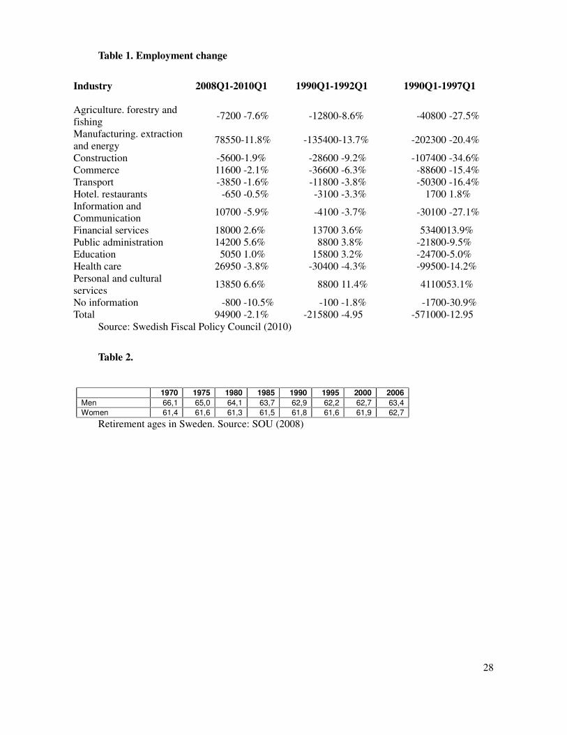
sectors. Table 1, shows that employment in several important sectors not only fell in the beginning

6

of the crisis, but employment continued to fall over the medium run horizon. This is, in particular

true for manufacturing, construction, commerce and the sectors dominated by public employment

like healthcare and public administration. Assuming some foresight among employers, it is not

difficult to understand that labor hoarding was not an option for a large share of employers during

the crisis in the 90s. In contrast, although employment has fallen in many sectors during the current

crisis, the bulk of the fall is accounted for by manufacturing. The total fall in employment between

2008Q1 and 2010Q1 was 94900 individuals, while the loss of employment in manufacturing was

78550 individuals. More importantly, while the loss in e.g., manufacturing employment in the 90s

turned out to be permanent, it seems more likely that employment will recover this time. Therefore,

the willingness to hoard labor should be much larger now, explaining the substantially weaker

relationship between the fall in output and the fall in employment which is key for the favorable

development of public finances despite the large fall in GDP.

Figure 5 provides more evidence in line with the argument of labor hoarding. The figure

shows that capacity utilization in manufacturing fell much more dramatically during the current

crisis. This indicates that the fall in output was to a larger extent than during the previous crisis

accounted for by a reduction in capacity utilization. During the crisis in the 90s, output instead

seems to have fallen due to permanent destruction of non-competitive jobs.

The conclusion from this section is that the comparatively favorable fiscal developments in

Sweden during the current crisis are not directly due to a high surplus and a low debt before the

crisis. Neither should the development be attributed to sheer luck. The new budgetary framework

and the care taken in not spending on ineffective stimulus packages did play an important role. But

the main explanation is that Swedish macroeconomic policy from the mid 90s had successfully

dealt with important structural problems. An extraordinary strong but not long-lasting negative

shock to the demand for Swedish export goods did therefore not lead to expectations of large and

7

costly structural changes. Therefore, important tax bases remained largely intact and the increased

demand for government transfers was manageable.

3. Room to maneuver – surpluses in good times and deficits in

bad

The key lesson from the previous section is that sound macroeconomic policies in general can

allow a country to withstand a very large negative shock without being seriously hurt in the short

and probably also in the medium and long run. Surpluses in good times and a not too large

government debt allowed expansionary fiscal policy and the full working of insurance systems that

help individuals hit by unemployment and other income reductions. A government budget that is

balanced or in surplus over the cycle leading to a small debt is therefore a necessary (but, as

stressed above, not sufficient) ingredient in a successful macroeconomic policy.

During the current crisis, as well as in many earlier instances of financial and economic crisis,

many countries have seen risk premia on their bonds rise quite dramatically, making it increasingly

costly to finance their debt. A key issue in the current debate is how large the surplus in good times

needs to be in order for deficits in bad times not to be so large as to be difficult to finance. There are

basically three ways the literature has dealt with this issue. The first is mainly concerned with

finding appropriate targets for the budget surplus over the business cycle, while the latter two deals

with government debt.

The first approach was taken by the Swedish government committee on stabilization policy

in a monetary union (Calmfors, 2002). Here, the idea is to base the surplus target on a maximum

accepted probability of the deficit becoming larger than the 3% threshold in the EU Growth and

Stability Pact. In the sub-report (Ohlsson, 2002), the distribution of GDP growth rates as well as the

8

sensitivity of the government deficit to changes in the GDP growth rate is estimated on Swedish

post-war data. Ohlson (2002) finds that a 1% decrease in the growth rates leads to a an increase in

the central government budget deficit of 0.8 or 1.2 percentage points of GDP, depending on whether

lagged GDP growth is included in the regression or not. He also finds that growth rates are

approximately normal with a mean of 2.7% and a standard deviation of 1.9%. If the target for the

average budget surplus over the business cycle is set to 2%, Ohlson calculates that the threshold

would be breached with a yearly probability of 0.2% (every 500 years on average) if the budget

sensitivity is 0.8 and with a yearly probability of 4.5% (every 24 years) if the sensitivity is 1.2.

In this year's report from the Swedish Fiscal Policy Council, it is argued that the calculations

reported above may overestimate the risk of breaching the 3% threshold since it is likely that the

surplus is higher than the target just before a crisis, given that surplus target applies over a full

business cycle. The starting point for the calculation should be something higher than the average,

allowing a larger fall than five percentage points it the target for the average surplus is two percent-

While this argument is formally correct, it appears more important to note that the normal

distribution is likely to be a bad approximation for the probability of extreme events. If the

assumption that growth rates are normal with mean 2.7% and standard deviation 1.9%, the

probability of the fall of Swedish GDP of 5% that occurred last year is so low as to happen only

once every 39500 years. If this is true, we certainly not need to take precaution for the possibility

that it happens soon again.

Another issue is that the budget sensitivity may not be a constant. As discussed in the

previous section, if a crisis also induces negative changes in the expectations of medium and long

run income and profits, the deficit can increase more when growth falls than under more normal

circumstances. The same is likely to be true if a recession coincides with large asset price

realignments. This did not happen in Sweden during the current crisis and the budget surplus and

9

GDP therefore fell around one for one. However, it is certainly not inconceivable that more negative

developments could occur again.

A second way of calculating appropriate fiscal policy targets focus on the debt and is taken in

a report to the Swedish Fiscal Policy Council this year (Bi and Leeper, 2010). Here, the purpose is

to construct a model that explains the risk premium as due to the risk that the government is unable

to repay its debt. The starting point is the fact that as for individuals, governments face what is often

called a natural borrowing limit. This limit exists since under reasonable assumptions, the

discounted value of future income minus necessary expenses is finite.2 A debt that is larger than this

amount is impossible to repay and no rational lender should lend when the debt approaches this

level. In the model of Bi and Leeper, stochastic elements imply that the probability that the

borrowing limit is approached is smoothly but non-linearly increasing in the current outstanding

debt. Calibrating the model to Swedish data, Bi and Leeper (2010) finds that the risk premium starts

increasing substantially at around 80% and that default is certain when the debt is around 100% of

GDP.

To give a quantitative perspective of this result, it is instructive to first note that fiscal

sustainability requires that the debt to GDP ratio is non-explosive. Focusing on balanced growth

paths, the debt to GDP ratio thus must converge to a constant. Now use the fact that the budget

constraint of the government can be written Bt+1 = (1+rt)Bt - Gt +Tt where Bt denotes government

debt, rt the interest rate, Gt government expenditures net of interest rate payments and Tt

government revenues, all measured in period t. Divide both sides of the equation by GDP and let

lower case b, g and t denote their uppercase counterparts, but expressed as ratios to GDP. Finally,

2 An exception would be if the economy is dynamically inefficient, i.e., when the steady state growth rate is higher

than the interest rate.

10

denote the growth rate of GDP by γ and consider a steady state where all variables are constant. We

then find that in a steady state, the debt to GDP ratio is constant and given by

b = (t-g)/(r-γ).

This equation can be used to calculate the natural borrowing limit by setting values to the

right-hand side parameters. A standard Laffer argument implies that t is bounded below unity –

there is a maximum share of GDP that the government can raise in taxes and other revenues and this

is strictly smaller than unity.3 Also g is bounded from below, at least at zero. These two observations

imply that the numerator in the right-hand side expressions have a maximum. Given the growth rate

γ and the interest rate r , assumed to be out of the governments control, this implies that there is a

maximum debt to gdp ratio, b, that can be maintained in steady state. The interpretation is that if the

outstanding debt is equal to this maximum, all taxes need to be set so as to maximize revenues (the

top of the Laffer curve) and government expenditures (net of interest rate payments) set to their

minimum in order for the debt ratio not to rise. Clearly, the debt can not be larger and if it reaches

this limit, it cannot be reduced.

Bi and Leeper use a more elaborate stochastic model, but the underlying argument is the same

– governments face a natural borrowing limit above which it must default. The problem with the

argument is that with quantitatively reasonable values of the parameters, the maximum debt is very

large. Suppose for example that it is economically possible for a government to run a permanent

primary surplus (t-g) of 5%. If this is done without changing Swedish government revenues at

around 55%, expenditures need to be cut to around 50%, which is well above the EU-average.

Clearly, this might be politically difficult, but is certainly not technically impossible. Suppose

3 In fact, Trabant and Uhlig (2009) use a calibrated model showing that the Swedish government is already close to this maximum.

11

furthermore that the long run difference between the nominal interest rate on government bonds and

the nominal growth rate is 1.5%, which if anything is a bit high. With this calibration, a debt of

0.05/0.015=3.33 can be sustained. It appears clear that a more realistic calibration would result in

much higher maximal debt levels. The reason why Bi and Leeper come to the opposite conclusion

is that they assume that the government cannot cut expenditures and that the interest rate is a whole

5 percentage point higher than the growth rate. These are unrealistic assumptions.

Given that technical inability to repay debt appears unlikely to explain default and risk premia

a third approach to studying debt and risk premia instead looks at default as a voluntary decision by

the debtor. Here, the decision maker weighs the costs and benefits of a default and default occurs if

the benefits dominate. Since the benefits tend to increases in the debt level, it is natural to

conjecture that, ceteris paribus, default probabilities increase in the current debt level.

A fundamental starting point for this literature on sovereign default is Bulow and Rogoff

(1989). They assume that the cost of default is permanent exclusion from borrowing. However, they

assume that a country that defaults can save at the world market interest rate. Although one in

principle could think that financial markets could coordinate so as to ban a defaulter also from

saving, it has an intuitive flavor that it would be possible also for a defaulter to place its saving

abroad. Given this assumption, Bulow and Rogoff show that exclusion from borrowing is never a

punishment sufficiently strong to prevent default. In fact, default happens with probability one and

no country should thus be able to borrow anything. The reason is that by defaulting and saving, a

higher consumption can always be achieved than if debt is honored. This result is labeled the

Bulow-Rogoff paradox.

In a growing literature, various solutions to the Bulow-Rogoff paradox have been proposed.

For example, Amador (2008) shows that political economy constraints may prevent saving after a

default and this makes default less attractive. Another explanation is used by Arellano

12

(2008), who assumes that default leads to a temporary output loss. She calibrates the model to

Argentina and shows that it can reproduce, in particular, the observed volatility of interest rate

spreads and defaults for Argentina. It does produce a fairly large average interest rate premium on

Argentinean debt that, however, falls short of the observed average risk premium unless a very high

degree of risk aversion among lenders is assumed.

The literature on sovereign default has provided important contributions to our understanding

of the quality and strength of default incentives faced by countries in emerging market and thus how

rational lenders should set default risk premia. However, we still lack similar quantitative models

for developed countries like Sweden. On the other hand, it seems reasonable that default is a

decision also in more advanced economies. Costs and benefits are weighed against each other,

albeit not necessarily by a benevolent country leader but instead in a political process. The lesson

for Sweden should then be that the relationship between debt levels and interest rate spreads is

highly dependent on how the market perceives the incentives for and against default. In part, this

might depend on basic political preferences that are hard to communicate to the market. Because of

the latter, reputation-building can be important – a country that is known to repay also when the

political and economic costs are high might be able to borrow more than a less trustworthy

government. Somewhat ironically, one might note that the Swedish crisis in 90s may have had long

run positive side-effects. Namely, it allowed Sweden to demonstrate that it repays its debt and is

able to deal with politically and economically costly restructuring if necessary.

Reputation is costly and takes time to build. Thus, also alternative institutional means to

decrease the perceived risk of default may be consider in order to shift out the relation between

interest rate spreads and debt. A starting point for an analysis of this is the inherent time-

inconsistency of borrowing. When taking up a loan, borrowers have an incentive to commit not to

be able to default (too easily) but ex ante, the incentive to breach these commitments increases and

13

may dominate. A standard remedy for problems like this has since the classic paper by Rogoff

(1985) been to delegate decisions to an agent with weaker incentives to give in to temptation. Here,

one might think of giving the decision on the budget to an independent fiscal board. Such a

delegation has been suggested to deal with the deficit-bias. Here, the standard counter-argument to

delegation is that it interferes with key political decision making. When discussing default

incentives rather than the deficit bias, this argument may be weaker. This since it does not seem

necessary to delegate in normal times but only in situations when the market starts to worry about

the default risk and interest rate spreads increase. Of course, delegation has to be legally prepared so

as to be possible to execute swiftly if deemed appropriate.

The issue of relaxing the relation between debt and interest rate spreads is particularly

important if other considerations, such as demographic changes, intergenerational equity and tax

smoothing call for a large debt buildup. However, the long-run forecasts of Sweden do not suggest

that a large debt buildup is optimal from either of these perspectives. If this is true, institutional

change to allow larger debt might be less of an issue.

4. Retirement

The issue of how taxes and transfers affect broadly defined labor supply is arguably the most

important issue in public finance, both from an efficiency point of view and for fiscal sustainability.

Broadly defined labor supply includes individual decisions among several margins. The two most

studied are the extensive margin whether to work or not and the intensive margin how many hours

per year to work. How these margins are affected by taxes and transfers is a very well researched

issue. Another key margin is the retirement decision. Here, the knowledge about how the retirement

decision responds to economic incentives is much smaller, not the least for Sweden. One of few

studies is Palme and Svensson (2003). By using micro data, they find that economic incentives are

14

important implying that that the construction the pension system, taxes and other transfers systems

that affect the retirement system are of key importance. The quantitative implications remain vague,

however, requiring intensified empirical work.

From 1970 to 1995, the average age at which Swedish males retired fell by four years from

66.1 t 62.2 years. At the same time the expected remaining lifetime at the 65 increased by close to 2

years from 14.1 to 15.9.4 During the decade thereafter, the retirement age increased by a year to

63.4 (in 2006) while the expected remaining lifetime increased by 1.5 years to 17.4. For females,

the average retirement age was fairly constant at around 61 years from 1970 to 1995 while the

trends in remaining lifetime was similar as that of men, with a steady increase from 17.5 to 20.6

from 1970 to 2006. 5

The increased longevity does not in itself imply that the socially optimal retirement age

should increase. This also depends on how the relation between productivity and health on the one

hand and age on the other has changed over time. However, it seems reasonable that also when

taking these factors into account, both passed and expected future increases in longevity should lead

to increases in the optimal retirement age.6 Under these assumptions, the trend-wise fall in the

retirement age during the period from 1970 to 1995 can be considered a policy failure due to poorly

constructed social insurance systems. The fact that the negative trends seem to have been broken

may be attributable to the pension reforms and other changes that have increased incentives to work

longer, as argued in the 2009 report from the Swedish Fiscal Policy Council.

The current pensions system with a defined contribution rate and automatic adjustments of

benefits to increased longevity provides fairly strong incentives for individuals to postpone their

4 Source: SOU (2008) 5 Source: SOU (2008) 6 If not, the current Swedish pension system with a fixed contribution rate seems poorly constructed. Instead, increased

longevity should lead to higher contribution rates.

15

exit into retirement. For a constant retirement age, a higher expected remaining lifetime leads to a

larger fall in income at retirement. However, it is clear that the retirement decision remains distorted

in the sense that the full value of the production generated by a marginal delay in retirement does

not accrue to the individual. It is also obvious that in an optimal (second best) allocation, one should

not aim for no distortions at this margin while other margins necessarily must remain distorted.

How strong incentives should be instead depends on how elastic the retirement decisions is with

respect to economic incentives relative to other labor supply margins. Given this, it is quite

unfortunate that we have so little knowledge about the retirement elasticity.

A general finding regarding the standard intensive and extensive labor supply elasticities is

that they depend a lot on individual characteristics. For example, the extensive margin is low for

prime age males with medium or high wages while it is substantially higher for women and low

wage individuals. Although, very little is known about the cross-sectional variation in the elasticity

of the retirement decision, one could not rule out that also here there is substantial variation. If there

are such differences, the incentives for staying in the labor force as average longevity increases

might need to be differentiated.

Recently, the Swedish National Government Employee Pensions Board (Statens

Tjänstepensionsverk), responsible for pensions to central government employees, reported a quite

substantial increase in the age at which state employees retire. As seen in Figure 6, the average age

of new retirees from state employment has increased by over 4 years for men and close to two years

for women over the last 10 years. This is substantially more than the average change in the Swedish

population. Although more evidence clearly is needed a tentative conclusion is that this change is

due to a particularly high elasticity of the retirement decision for male state employees.

It is well known that individuals with higher education tend to retire later (Burtless, 2008 and

Gutiérrez-Domènech, 2006). The findings regarding the strong increase in the retirement age for

16

state employees also indicate that the responsiveness to economic incentives vary across groups.

The stronger work incentives for people above 65 seem to have not only increased the average

retirement age but also increased the cross sectional variability as pointed out in SOU, (2008). This

also points in the direction of substantial cross-sectional differences in the sensitivity to economic

incentives.

A high cross-sectional variation in the retirement age elasticity indicates a policy problem. On

the one hand, incentives to work longer are required for long-run fiscal sustainability. Such

incentives reward late retirement relative to early. It is likely that unchanged behavior needs not

only to be punished relatively but also absolutely. In any case, the outcome of stronger incentives

for late retirement is likely to be a potentially large increase in interpersonal differences in life time

income and consumption. This calls for more differentiated pension rules. In a world of perfect

information, individuals with a high elasticity of the retirement age should be given strong

incentives to work long. Punishing them for retiring early has no welfare cost since they simply

retire later. On the other hand, individuals whose retirement decision is less elastic should not be

punished for retiring early. Obviously, this problem is not new and attempts to mitigate it include

systems for disability pension or sick pension or early pension due to bad labor market conditions.

Previous experience with these systems shows the difficulty in designing such systems. Many of the

reasons for why a person has a special need to retire earlier than others are difficult to verify

objectively.

More knowledge is needed before clear policy conclusions can be drawn. In particular, it is

important to know how the elasticity of the retirement decision varies between different individuals.

However, it seems likely that the tension increases between on the one hand the goal of providing

incentives for those who can work long to do so and on the other, providing insurance to those who

cannot work long. When the characteristics driving the differences in the potential for later

17

retirement are observable, they should be allowed to affect pension rules. A system with more

differentiation across occupations as regards to the normal retirement age and the age at which

health insurance and job security stop being in effect might be a reasonable way to go.

The discussion above has implicitly assumed that differences in the elasticity of the retirement

age depend on characteristics of the individual and her job. However, it is possible that also

differences in access to alternative means of income, like private pension plans can be part of the

explanation. If that is the case, it is likely to affect the policy conclusions. It is therefore also of key

importance to get a better understanding of why the elasticity of the retirement decision varies

between individuals.

5. Cyclical Variation in the Unemployment Insurance

The U.S. and Canada have procedures for changing the rules of the unemployment insurance

system over the business cycle. Specifically, the maximum duration of benefits increases if regional

unemployment rates increase beyond particular thresholds. In addition to this automatic response,

congress often makes discretionary decisions on duration extension when the economy is in

recession. The cyclical variation in generosity is fairly large, in particular in the U.S., where the

maximal duration may be almost doubled from the regular 26 weeks.

There are theoretical reasons for having a cyclical variation in the unemployment insurance.

The basic microeconomic tradeoff when constructing efficient unemployment insurance is between

providing insurance, on the one hand, and providing incentives to search for a new job on the other.

There are reasons to believe that this tradeoff may vary over the cycle. If a recession leads to high

unemployment and few vacancies, the value of inducing high search effort may fall while the value

of providing insurance increases. This change in the tradeoff would call for a more generous

unemployment insurance and, perhaps in particular, a slower reduction in benefits over the

18

individual unemployment duration when the economy is in recession (see Sanchez, J. M., 2008).

Michalat (2010) constructs a model where unemployment is due both to wage rigidity and to

search frictions. The author proposes a decomposition of unemployment such that the part due to

wage rigidity is defined as the unemployment rate that would result if recruiting costs were zero and

the remainder is defined as frictional unemployment. By calibrating the model to U.S. data it is

shown that the shares of the two components vary dramatically over the cycle. When

unemployment is below 5% it is only frictional but when it reaches 9%, the frictional component

only accounts for 2 percentage points. As stated by the author “in bad times, there are too few jobs,

the labor market is slack, recruiting is inexpensive, and matching frictions contribute little to

unemployment.”

The Swedish Fiscal Policy Council last year proposed the introduction of an automatic

mechanism that increases the duration of the initial period of unemployment benefits at 80% of the

previous wage. The increase should be triggered if the unemployment rate is above a particular

threshold and it is higher than previous year’s unemployment rate by a given amount. The latter

criterion is also included in the U.S. and Canadian systems and is in a rough manor meant to capture

the possibility of variations in the natural rate of unemployment.

The results by Michalat (2010) seem to support the proposal of the Fiscal Policy Council.

However, one should bear in mind that the macroeconomic consequences of the introduction of a

U.S./Canadian system in Sweden and the U.S. may be quite different.7 First, the natural rate appears

more stable in the U.S. than in Sweden. The criterion that unemployment must have increased

relative to last year is therefore a quite inadequate fix for variations in the natural rate, making the

7 Note though, that the proposed variability is small relative to the case in the U.S. The proposal is to let the point in time when benefits are cut from 80 to 70% vary over the cycle. In the U.S., it is the time when benefits go to zero that changes.

19

automatic system more problematic in Sweden.

Second, the consequences for wage formation of increased unemployment generosity may be

different and possibly larger in Sweden than in the U.S. This since unions play a substantially more

important role and the unemployment insurance is already more generous in Sweden. The risk and

cost of increasing the natural rates and the share of long term unemployed is likely to be higher in

Sweden.

The current recession in Sweden is not due to domestic problems regarding wage formation,

as discussed above. Partly because of this, it would probably have been socially beneficial to

temporarily increase unemployment benefits during the last year when unemployment rates shot up

and the expectation was that large industrial restructuring was not necessary. During the crisis in the

90s, the situation was quite different and a temporary increase in benefits may then have been more

problematic. Introducing an automatic system of variations in benefit generosity may therefore be

worse than having some discretion. A possible alternative is to have a system that allows temporary

increases in generosity that are automatically rolled back in a pre-specified way.

Blanchard and Tirole (2008) discuss an arguably more fundamental problem in designing

good unemployment insurance systems. They note that publically funded unemployment insurance

implicitly subsidizes layoffs.. To understand their argument, think of the cost of unemployment

benefits born by the tax payers as an externality. By laying off a worker, the firm induces costs on

tax payers. Since these costs are not internalized by the firm (nor by the worker) too many layoffs

are likely to result. This effect can be counteracted by various forms of employment protection but

Blanchard and Tirole (2008) argue convincingly that a layoff tax, equal in value to the expected

unemployment benefits paid by the government, is the most direct way of making firms internalize

the cost a layoff inflicts on the government’s budget. It is also important to note, that severance

payments from the firm to the worker does not do the trick since it simply makes the

20

worker more willing to accept a layoff by changing the division of costs between the worker and the

firm. To induce the right behavior, the firm and the worker must together bear the externality cost.

In Sweden, firms can fairly easily and cheaply reduce their workforce by layoffs. Unless firms

make an agreement with the unions, they must follow the principle of last in, first out. However,

unions have an incentive to accept reasonable deviations from this rule. Therefore, it seems

reasonable to argue that the cost of layoffs is low, potentially leading to a too high rate of layoffs in

business cycle downturns. In a downturn as the 2008-9 crisis, when export demand for Swedish

goods fell dramatically, one could argue that the reduction in hours worked should have been shared

more equally over the relevant workforce. Instead, the implicit subsidy to layoffs may have lead to a

concentration of this reduction to a smaller number of individuals who are forced to stop working

altogether, while the remaining worker work full time. In an attempt to counteract this, the large

union IF Metall, with around 400 000 members mostly in manufacturing, in March 2009 made a

work sharing agreement with the employer’s federation. According to the agreement individual

firms can be allowed to make temporary reductions in both work and pay with up to 20%.

According to the yearly report from the National Mediation Office (Medlingsintitutet 2010),

around half of the firms in metal and vehicle industries made temporary work sharing agreements.

According to the same report, the employers estimate that the agreement has led to more than 10

000 workers remain employed in the current crisis.

It seems important to stimulate work sharing agreements, possibly also by introducing a

system of temporary subsidies to work sharing agreements in recessions. It is also important to

realize that the value of work sharing is likely to be countercyclical. Permanent subsidies to work

sharing may reduce structural change and thereby hamper long-run growth and should therefore not

be considered.

21

6. Concluding summary

Sweden has fared well in the current crisis relative to its previous experience and in

comparison to many other countries. The reason for this is partly that Sweden had sound public

finances before the crisis with a quite high surplus and low debt. The main reason is, however, that

sound macroeconomic policies over the period from the crisis in the 90’s until today had made

Sweden able to endure a temporary shock to export demand without large other repercussions. The

fiscal surplus was as higher in 1990 than in 2007, but this did not help much when crisis hit in the

90’s since that crisis made it apparent that the Swedish economy needed a complete overhaul. Such

structural change takes time, is costly and puts a great strain on all parts of the economy.

The current fiscal policy framework, including a surplus target of 1% over the cycle should be

maintained, but is not a substitute for good general macroeconomic policies. The current and

previous governments have demonstrated a strong commitment to fiscal responsibility. This is a

substantial asset for Sweden. The ability for a government to borrow in economic downturns is

typically not much limited by its economic capacity. Rather, the critical issue is whether lenders

believe that governments and voters want to pay back government debt. The relationship between

spreads on government debt and the debt level is therefore not stable enough to allow simple rules

to prevent fiscal crisis.

A key issue for fiscal sustainability is that the share of total life spent working does not

deteriorate. Given that time spend in education is likely to continue to increase, the average

retirement age should increase. Recent developments in Sweden have demonstrated that the

decision when to retire does respond to economic incentives. Reforms that have increased the

returns to working seem to have been important for the increase in the retirement age among in

particular government employees. However, stronger economic incentives usually come at the cost

of less insurance. Regarding retirement, the risk is that the necessary strengthening of incentives to

22

work increases the intra-individual spread in lifetime income. It is therefore important to monitor

this development and possibly allow a larger differentiation across occupational groups, giving

stronger incentives to retire late in occupations where a long working life is reasonable but allow

earlier retirement with adequate benefits in other occupations.

The final issue addressed in this report is if the rules in the unemployment insurance system

should be automatically varied over the business cycle. One can make the argument that the tradeoff

between insurance and incentives is likely to vary over the business cycle. A similar, and perhaps

stronger argument, can be made for policies that facilitate work sharing. A complication, however,

is that not all business cycles are the like. Increasing unemployment benefits does effect wage

formation and how negative the consequences of this is for job creation is not the same in every

downturn. This calls for caution, at least for radical reform.

References

Amador, Manuel, (2008), “Sovereign Debt and The Tragedy of the Commons”, unpublished

manuscript, Stanford University.

Arellano, Cristina, “Default Risk and Income Fluctuations in Emerging Economies",

American Economic Review, June 2008, 98 (3).

Bi, Huixin and Eric M. Leeper, (2010), “Sovereign Debt Risk Premia and Fiscal Policy in

Sweden”, Studier i Finanspolitik 2010/3, Swedish Fiscal Policy Council

Blanchard, Olivier and Jean Tirole, (2008), 2The Joint Design of Unemployment Insurance

and Employment Protection: A First Pass”, Journal of the European Economic Association, Vol. 6:1.

Boije, Robert, Jonas Norlin, Albin Kanelainen and Hanna Ågren, (2010,) ”Utvärdering av

överskottsmålet”, DS 2010:4, Ministru of Finance, Swedish Government

Bulow Jeremy and Kenneth Rogoff, (1989), “Sovereign Debt: Is to Forgive to

23

Forget?”, American Economic Review, March 1989, v. 79, iss. 1, pp. 43-50.

Burtless, Gary, (2008), “The Rising Age at Retierment in Industrial Countries”, Center for

Retirement Research at Boston College, WP 2008-6.

Calmfors, Lars, (2002), “Stabiliseringspolitik i valutaunionen, slutbetänkande”, SOU

2002:16, Fritzes, Stockholm.

Gutiérrez-Domènech, Maria, (2006), ”The Employment of Older Workers”, la Caixa Working

Paper Series, 4/2006.

Medlingsinstitutet, (2010), “Avtalsrörelsen och lönebildningen 2009”, yearly report from The

Swedish National Mediation Office.

Michaillat, Pascal, (2010), “Do Search Frictions Explain Unemployment? Not in Bad Times”,

unpublished manuscript, University of California, Berkley.

NIER (2005), Konjunkturläget Mars 2005, Konjunkturinstitutet.

NIER (2010), Konjunkturläget Juni 2010, Konjunkturinstitutet.

Ohlsson, Henry, (2002), ”Finanspolitik i en valutaunion”, bilaga 4, SOU 2002:16, Fritzes,

Stockholm.

Palme, Mårten and Ingemar Svensson, (2003), “Pathways to Retirement and Retirement

Incentives in Sweden”. in T. Andersen and P. Molander (eds.) Alternatives for Welfare Policy,

Cambridge University Press: Cambridge.

Rogoff, K (1985), ‘The optimal degree of commitment to an intermediate monetary target’,

Quarterly Journal of Economics, November, p. 169–90.

Sanchez, J. M. (2008), “Optimal state-contingent unemployment insurance”, Economics

Letters 98.

24

SOU, (2008), Långtidsutredningen, SOU 2008:105, Fritzes, Stockholm.

SPV, (2009), Pensionsstatistik 2008, Statens Pensionsverk.

Swedish Fiscal Policy Council, (2010), “Svensk Finanspolitik – Finanspolitiska rådets rapport

2010” (in Swedish).

Trabandt, Mathias and Harald Uhlig, (2009). ”How far are we from the slippery slope? The

Laffer curve revisited”, NBER WP 15343.

25

Figure 1. Real GDP relative to value before crises during 90's crises and current crisis.

2008:1=100 1990:1=100Forecast

Source: Swedish Fiscal Policy Council (2010).

Figure 2. General government net lending.

-14,0

-12,0

-10,0

-8,0

-6,0

-4,0

-2,0

0,0

2,0

4,0

6,0

1980

1982

1984

1986

1988

1990

1992

1994

1996

1998

2000

2002

2004

2006

2008

2010

2012

Source: NIER (2005, 2010).

26

Figure 3. General Government Gross Debt (Maastricht definition)

0

10

20

30

40

50

60

70

80

1980

1982

1984

1986

1988

1990

1992

1994

1996

1998

2000

2002

2004

2006

2008

2010

2012

Source: NIER (2010)

Figure 4. General Government Net financial Assets

-30

-20

-10

0

10

20

30

1993

1994

1995

1996

1997

1998

1999

2000

2001

2002

2003

2004

2005

2006

2007

2008

2009

2010

2011

2012

Source: NIER (2010)

27

Figure 5. Capacity utilization in Manufacturing

70,0

75,0

80,0

85,0

90,0

95,0

1991

1991

,8

1992

,5

1993

,319

94

1994

,8

1995

,5

1996

,319

97

1997

,8

1998

,5

1999

,320

00

2000

,8

2001

,5

2002

,320

03

2003

,8

2004

,5

2005

,320

06

2006

,8

2007

,5

2008

,320

09

2009

,8

Source: NIER (2010).

Figure 6. Average age of new state employee retirees

Females Males

Retirement age

Source: SPV (2009)

28

Table 1. Employment change

Industry 2008Q1-2010Q1 1990Q1-1992Q1 1990Q1-1997Q1

Agriculture. forestry and fishing

-7200 -7.6% -12800-8.6% -40800 -27.5%

Manufacturing. extraction and energy

78550-11.8% -135400-13.7% -202300 -20.4%

Construction -5600-1.9% -28600 -9.2% -107400 -34.6% Commerce 11600 -2.1% -36600 -6.3% -88600 -15.4% Transport -3850 -1.6% -11800 -3.8% -50300 -16.4% Hotel. restaurants -650 -0.5% -3100 -3.3% 1700 1.8% Information and Communication

10700 -5.9% -4100 -3.7% -30100 -27.1%

Financial services 18000 2.6% 13700 3.6% 53400 13.9% Public administration 14200 5.6% 8800 3.8% -21800 -9.5% Education 5050 1.0% 15800 3.2% -24700 -5.0% Health care 26950 -3.8% -30400 -4.3% -99500 -14.2% Personal and cultural services

13850 6.6% 8800 11.4% 41100 53.1%

No information -800 -10.5% -100 -1.8% -1700 -30.9% Total 94900 -2.1% -215800 -4.95 -571000 -12.95

Source: Swedish Fiscal Policy Council (2010)

Table 2.

1970 1975 1980 1985 1990 1995 2000 2006

Men 66,1 65,0 64,1 63,7 62,9 62,2 62,7 63,4

Women 61,4 61,6 61,3 61,5 61,8 61,6 61,9 62,7

Retirement ages in Sweden. Source: SOU (2008)