Embed Size (px)
Citation preview

Productivity Tools for Autodesk® Civil 3D® ANZ
Civil 3D Productivity Tools for ANZ Civil 3D Productivity Tools for ANZ is a suite of customised add-ins to allow more
productive design and documentation of your Civil 3D projects.
The tools cover a broad range of tasks, including:
• Aquaplaning analysis
• Annotating of Section Views (including corridor point cuts and staggering)
• Exporting flattened 2D AutoCAD drawings from a 3D GENIO import
• Exporting corridors and featurelines for construction
• Create roadside barriers in 3D
• Exporting Featurelines to 3D XYZ coordinates
• Copy Data Band Profile parameters
• Adjusting datum levels on multiple Profile Views
These tools currently reside in the Toolbox folder located at:
%LocalAppData%\\Autodesk\C3D <version>\enu\Data\ToolBox\ANZ

Contents Civil 3D Productivity Tools for ANZ ...................................................................................................... 1
Civil 3D Drip ........................................................................................................................................... 3
Civil 3D SectionLabel ......................................................................................................................... 13
Civil 3D Genio2D .................................................................................................................................. 21
Civil 3D ExportForConstruction .......................................................................................................28
Civil 3D Barriers ................................................................................................................................. 34
Civil 3D Export Feature Lines XYZ .................................................................................................. 39

Civil 3D Drip Drip allows users to perform immediate on-screen aquaplaning calculations through a
custom dialog. The user selects a Civil 3D surface object, a point to analyse and a
terminating (or break) string. The program will determine the flow path and calculate the
aquaplaning depths for each segment along the flow path in accordance to Austroads
Guide to Road Design Part 5a – Section 4 (Aquaplaning).
The resulting aquaplaning calculation is shown on-screen through a series of coloured
bands (green, orange and red) to indicate whether issues exist on the surface.
This output can finally be output to Excel for use in design reports.
General Notes
• A Point Code Terminator is required to run the analysis, regardless of whether a
terminator is required or not. This issue will be addressed in a future release.
• It is recommended to turn on viewport lineweights (in the status bar) to
better visualise the flow paths.
• The Drip add-in will create an XML file, called ‘Drip.xml’, in the same folder where
the current drawing is located. The XML file will read and write settings so when
the program is re-run, the latest settings in the dialog are not lost.
• The analysis result shown in the bottom portion of the dialog (after clicking ‘Drip’)
is a simplified analysis that utilises the Gallaway method (1979), and uses the
average length and slope of the entire flow path (i.e. point to point). Detailed
analysis results are found in the generated Excel report.
• To get a better aquaplaning result, it is preferred to create a corridor region
through the aquaplaning analysis zone with lower region frequencies (i.e. 1-2m).
This creates a smoother triangulation used to calculate the waterdrop flow path.

Loading
Navigate to the Toolspace – Toolbox - Australia and New Zealand Reports Manager – ANZ
Tools – Drip (Aquaplaning), and either right-click and select ‘Execute’ or double-click the
left mouse button to run the command.
Figure 1: Drip dialog

Process
Surface
The surface pulldown lists all surfaces in the drawing. The currently selected surface is
the surface the analysis will be run on.
Figure 2: Selecting a surface
Coordinates
Coordinates are used to select the upstream flow path point on the Surface (see above).
Values can be entered directly into the X and Y boxes, or simply clicking the icon.
Once the point selection icon is selected, a point can then be selected directly on screen.
Points are selected on screen by using the left-click button. Clicking on the surface will
display a thick blue line indicating the selected flow path (running from the selected
upstream point to the downstream end, stopping at the low point on the surface)
If the selected point does not lie on the surface, a red cross marker will appear.
To finalise and confirm the selected point, either right-click the mouse button. The X and
Y coordinates in the Drip dialog will update to reflect the new analysis point.
Figure 3: Point selection on surface (left) and invalid point selection (right)

Aquaplaning Point Code Terminator
The Point Code Terminator is a selected feature line from the underlying corridor model,
and a related Intersection Number will determine where the two strings (Point Code
Terminator and the Water Drop flow path) intersect.
Typically, when a flow-path is selected, the initial flow path runs from the selected
upstream point to the surfaces low-point. This full-length line is not typically used for the
analysis, as the waterdrop will typically stop at a feature on the pavement (i.e.
linemarking edge, lip of kerb etc). The image below shows this scenario.
Figure 4: Point Code Terminator
Once the Point Code Terminator icon is selected, a feature line can be selected from a
corridor model. This corridor model is typical the same one used to generate the surface
for the analysis.
At the command prompt, select either a CorridorFeatureLine or FeatureLine on-screen. If
a CorridorFeatureLine is selected and the cursor detects more than one featureline under
the cursor, a list will appear prompting the Feature Line section. Double click the feature
or highlight the line or select OK to confirm.

Figure 5: Select A Corridor Feature Line
On confirmation of a selected Feature Line, the textbox next to the Point Code Terminator
will display the Corridor name followed by the feature line name, separated by a ‘->’
symbol (i.e. CORR-MAIN->CE)
Figure 6: Point Code Terminator and Intersection Number
The Intersection Number is an integer value calculating when and how many times the
two lines intersect (flow path and feature line). For instance, an Intersection Number of 0
indicates that the entire flow path string will be used for the analysis. In the image below,
the Intersection Number of 1 is used to terminate the analysis at the first intersection
point between the water drop and the featureline.
Figure 7: Intersection Number 1 selected for analysis

Aquaplaning Parameters
Aquaplaning parameters are used to calculate the flow path analysis and are described
below.
Figure 8: Aquaplaning Paramteres
Texture Depth (mm)
Refers to the average depth of the macrotexture of the road surface.
Figure 9: Pavement Texture Depth
Rainfall Intensity (mm/hr)
For design, rainfall intensity is determined from an appropriate rainfall intensity-
frequency-duration (IFD) chart for a particular site, using a selected ARI and appropriate
duration.
Design Speed (km/h)
A design speed is selected from the drop-down menu. Design speeds range from 30km/h
to 120km/h. The design speeds, in conjunction with the ‘Friction Demand High’ checkbox,
determine the overall Aquaplaning Limit
Figure 10: Design Speeds
Friction Demand High?

This checkbox is used where the friction demand is high, such as at intersections, steep
downhill grades or where the road design speed is 80km/h or higher. See Section 4.10.1 in
Austroads Part 5a: Drainage – Road Surface, Networks, Basins and Subsurface for more
details.
Aquaplaning Limit (mm)
The Aquaplaning limit is a read-only value calculated from a combination oft design
speed and Friction Demand. The values fall between 4mm and 5mm.
Analysis
Aquaplaning analysis is performed by left-clicking the ‘Drip’ button in the upper-right
corner of the dialog.
It is required to have all elements in the dialog populated before a successful analysis is
calculated.
Figure 11: 'Drip' Analysis button
Analysis results are displayed on-screen as a thick polyline, with color bands indicating
successful or non-successful aquaplaning calculations. Note the original blue flow path is
removed from screen upon running the analysis.
Figure 12: Analysis result on-screen

The analysis result shown in the bottom portion of the dialog (after running a ‘Drip’
analysis) is a simplified analysis that utilises the Gallaway method (1979) and uses the
average length and slope of the entire flow path (i.e. point to point). Detailed analysis
results are found in the generated Excel report.
Figure 13: Point to Point analysis (simplified)
The image below shows a successful aquaplaning analysis on a corridor design surface
using the following design parameters:
• Right-edge lip as the Point Code Terminator (CORR-MAIN->CE)
o Intersection Number 1
• Texture Depth 0.4mm
• Rainfall Intensity 50mm/hr
• Design Speed 80km/h
• Friction Demand High? Yes
• Aquaplaning Limit 4mm
Figure 14: Successful aquaplaning analysis

The image below shows an unsuccessful aquaplaning analysis on a corridor design
surface using the following design parameters:
• Right-edge lip as the Point Code Terminator (CORR-MAIN->CE)
o Intersection Number 1
• Texture Depth 0.4mm
• Rainfall Intensity 120mm/hr
• Design Speed 80km/h
• Friction Demand High? Yes
• Aquaplaning Limit 4mm
Figure 15: Unsuccessful aquaplaning analysis
Reporting
Upon completion of an analysis. Select the ‘Report’ button in the bottom-right of the
dialog. This will create an Excel file (called ‘Drip.xlsx’), which can then be saved in another
location (Save-As) for use in reports
Figure 16: Reporting to Excel

The Excel report includes all calculation information, including charts and a table of the
calculation segments.
Figure 17: Sample Excel report
Civil 3D SectionLabel SectionLabel will allow the user to select a single Section View (as part of a Section View
Group) and annotate user-defined point codes within data bands, allowing for staggering
of overlapping text labels.
Steps to be considered when using the SectionLabel tool:
• Use a Code Set Style to add point code labels to a Corridor Section on a Section
View. The SectionLabel tool will only annotate Corridor Sections (i.e. not Surface
Sections). See ‘Section View Corridor Sections - Code Set Style’ for more details.
• Add Data Bands to Section View(s). See ‘Section View Data Bands’ for more details.
• Edit the Section View Style description to add/remove specific customised Section
View attributes (no ticks, XYZ annotation etc). See ‘Section View Style’ for more
details.
• Select a single Section View contained in the Section View Group
The program relies on specific coding standards and Civil 3D Settings that the user must
conform with to successfully use the add-in.
General
• The Section Views must be part of a Section View Group (no Individual Sections)
• To scale the text in the data bands correctly, the system variable ‘Measurement’
should be set to ‘0’ for Imperial and ‘1’ for Metric
Loading
Navigate to the Toolspace – Australia and New Zealand
Reports Manager – ANZ Tools – Section View Labels, and
either right-click and select ‘Execute’ or double-click the left
mouse button to run the command.

Section View Corridor Sections - Code Set Style
The SectionLabel add-in annotates only Corridor Sections displayed on a Section View.
Surface Sections are not used to label the specific point codes, except for the existing
surface, which is used to extract levels at the Corridor Section cut offset locations.
To annotate labels on Corridor Sections, the Corridor Section Code Set Style must be
setup for the section labels to be cut.
1. Assign a Code Set Style to the Corridor Sections
Figure 18- Assign Code Set Style to Corridor Sections
Figure 19 - Starting point for Section View labelling

2. Edit the Code Set Style.
To determine which labels to annotate, edit the Code Set Style.
Under the Point category, assign a Label Style called ‘ADSK_SectionLabel’ (not
case sensitive). This tells the program which codes to annotate. For example, in the
image below, the codes CB, CE, CF and CT will be labelled through the program.
a. Additionally, assigning a label style called ‘ADSK_SectionLabel_Sub’ will
allow you to annotate a separate set of points along the Subgrade (or
Datum) data band, separate from the top surface design strings.
3. Optionally, add a value to the Points ‘Description’ column to override the value of
the feature label in the data band.
4. Note: ‘ADSK_SectionLabel’ and ‘ADSK_SectionLabel_Sub’ labels are design for use
in the SectionLabel tool only. It is recommended to place the resulting Section
View objects onto non-plotting layers
Figure 20 - Adding Label Styles to determine Section View annotation

Section View Styles
• In the Section View Styles dialog, adding the text string ‘#XYZ’ to the description
box annotate the master baseline (alignment) label just above the datum (LHS)
Figure 21- Adding XYZ annotation to Section View

Section View Data Bands
The SectionLabel add-in annotates all specified text values within existing Section View
Data Bands, including labelling the existing surface at the same ‘cut’ locations, specified
by the user. To avoid excessive user-interface, the program is hard-coded to search
through all Section View Data Bands in your DWG file, and return text information (height,
style etc.) that matches any of the following naming criteria. Note the data band labels
only have to contain any of the following text strings and is not case sensitive.
1. Name the Data Bands in accordance with the following criteria
Section View – Band Styles – Section Data - Data Band Names
o Feature Lines / Codes
▪ ‘FEAT’
▪ ‘LABEL’
▪ ‘CODE’
o Design Levels
▪ ‘DESI’
▪ ‘PROP’
o Existing Levels
▪ ‘EXISTING’
▪ ‘NATU’
o Offset
▪ ‘OFF’
▪ ‘DIST’
o Subgrade/Datum
▪ ‘SUB’
▪ ‘STRAT’
▪ ‘DATUM’
Figure 22- Data Band Naming Convention

2. In the Section Data Band Style dialog, edit the Data Band text style through the
‘Summary’ tab – Band Details – Band Text Style.
Figure 23 - Edit Data Band Text Style
3. In the Section Data Band Style dialog, edit the Data Band text height through the
‘Band Details’ tab – Grade Breaks – Compose Label.
Figure 24 - Edit the Data Band Text Height (through Grade Breaks)

a. In the Label Style Composer, add a Text Component, and change its text
height value. The add-in will read this value and set the text heights for the
data band.
Figure 25 - Changing the Data Band Text Height property
4. Inside the Section Data Band Style dialog, adding the text string ‘#NoTicks’ into
the Description will remove ticks from the Data Band

Surfaces
The SectionLabel add-in annotates an existing (or natural) surface at the same ‘cut’
locations as specified by the user. To avoid excessive user-interface, the program is hard-
coded to search through all TIN surfaces in your DWG file, and return the first surface that
matches any of the following naming criteria. Note the surface only has to contain any of
the following text strings and is not case sensitive.
• ‘EX’
• ‘EG’
• ‘GROU’
• ‘TERR‘
• ‘NGL’
• ‘TX’
• ‘SURV’
• ‘NATU’
For example, a surface called ‘Existing Ground’ will be returned, as it contains ‘EX’ and
‘GROU’ within the name.
Figure 26 - Remove ticks from a Data Band
Civil 3D Genio2D Genio2D allows users to take a 3D Genio import (from the Autodesk® Import-Export
Extension for GENIO) and create a flattened 2D version of the file for Xref underlays and
CAD exports.
This add-in will convert all 3D elements based on layer and object type. 3D Linework and
COGO points are all converted to their relative 2D polyline and block counterparts through
a text mapping file (*.txt)
GENIO (General Input-Output) is a text-based file format developed for exchanging data
between MOSS/MX and other design packages.
The current version of the product is setup for RMS workflows (although the add-in can
be customised to suit any region).
Future releases will include functionality for other regions.
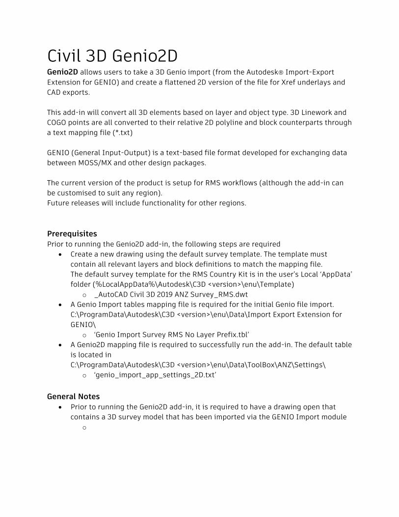
Prerequisites
Prior to running the Genio2D add-in, the following steps are required
• Create a new drawing using the default survey template. The template must
contain all relevant layers and block definitions to match the mapping file.
The default survey template for the RMS Country Kit is in the user’s Local ‘AppData’
folder (%LocalAppData%\Autodesk\C3D <version>\enu\Template)
o _AutoCAD Civil 3D 2019 ANZ Survey_RMS.dwt
• A Genio Import tables mapping file is required for the initial Genio file import.
C:\ProgramData\Autodesk\C3D <version>\enu\Data\Import Export Extension for
GENIO\
o ‘Genio Import Survey RMS No Layer Prefix.tbl’
• A Genio2D mapping file is required to successfully run the add-in. The default table
is located in
C:\ProgramData\Autodesk\C3D <version>\enu\Data\ToolBox\ANZ\Settings\
o ‘genio_import_app_settings_2D.txt’
General Notes
• Prior to running the Genio2D add-in, it is required to have a drawing open that
contains a 3D survey model that has been imported via the GENIO Import module
o

Loading
Navigate to the Toolspace – Toolbox - Australia and New Zealand Reports Manager – ANZ
Tools – Genio 2D, and either right-click and select ‘Execute’ or double-click the left mouse
button to run the command.
Figure 27: Genio 2D Loader

Process
Create a new drawing
Create a new file using the default survey template (File – New). This DWT should will
contain the layers and block for local standards.
For example, the image below shows a new file created from template ‘_AutoCAD Civil 3D
2019 ANZ Survey_RMS.dwt’
Delete any linework and blocks from the new drawing, as these are at origin (0,0) and for
display purposes only.
Figure 28: New file with survey template

Import a GENIO file
The Autodesk® Import-Export Extension for GENIO is a separate add-in provided with
Civil 3D to subscription customers, and can be downloaded from the user’s Autodesk
Account page (https://manage.autodesk.com/)
The installation guide is located
https://up.autodesk.com/2019/CIV3D/GENIOExtension2019.htm
The image below shows the GENIO extension on the Autodesk Accounts page
1. https://manage.autodesk.com/
2. Login
3. Product Updates
4. Search for ‘GENIO’
5. Download (if available)
Figure 29: GENIO download from Autodesk Accounts page

• From the Toolbox, navigate and select ‘Subscription Extension Manager –
Autodesk® Import-Export Extension for GENIO – Import from GENIO…’
• Update or check the ‘GENIO Import Options’ tab, and load the String Label Layer
Table ‘Genio Import Survey RMS No Layer Prefix.tbl’, which is installed as part of
the ANZ Country Kit
Figure 30: GENIO Import Options
• In the ‘GENIO Import Selection’ tab,

o Open the Genio file
o Select the Genio file from the left column (Models)
o Select the strings to import from the right column (Strings)
o Click ‘Import’
Figure 31: GENIO Import Selection
• The imported Genio provides 3D Polylines and COGO Points
Figure 32: GENIO Import 3D Polylines and COGO Points
Convert the drawing to 2D

• Run the Genio2D add-in from the Toolbox (described above)
• A warning dialog will ask if you wish to proceed. Please note that all 3D polylines
and COGO points are deleted (or converted) into a 2D Polylines, Block References
and MText.
• Click ‘Yes’
• This applied mapping file is in a subfolder (called \Settings\) under the add-in
installation folder, for example, the executable file in:
o C:\ProgramData\Autodesk\C3D <version>\enu\Data\ToolBox\ANZ\
Autodesk.Consulting.Civil3D.Genio2D.<version>.dll
Looks for a mapping file in the folder:
o C:\ProgramData\Autodesk\C3D <version>\enu\Data\ToolBox\ANZ\Settings\
‘genio_import_app_settings_2D.txt’
• Save the drawing and open it again to see all the block references applied
correctly.
• This drawing is now ready to be used as a 2D representation of the survey Genio.

Civil 3D ExportForConstruction ExportForConstruction allows users to export Corridor Feature Lines and Site Feature
Lines into a new AutoCAD drawing as a 2D or 3D drawing.
Prerequisites
Prior to running the Export add-in, the following steps are required
• The drawings should contain either:
o One (1) Corridor containing feature line(s)
o One or more ground Feature Lines
General Notes
• The ExportForConstruction add-in will create an XML file, called
‘ExportForConstruction.xml’, in the same folder where the current drawing is
located. The XML file will read and write settings so when the program is re-run,
the latest settings in the dialog are not lost.

Loading
Navigate to the Toolspace – Toolbox - Australia and New Zealand Reports Manager – ANZ
Tools – Export For Construction ANZ, and either right-click and select ‘Execute’ or double-
click the left mouse button to run the command.
Figure 34: Corridor Feature Lines and Site Feature Lines
Figure 33: Export For Construction Loader

Process
Run the Genio2D add-in from the Toolbox (described above)

Corridors
The ExportForConstruction add-in will allow exporting from either multiple corridors or
allow selection of a single corridor.
The drop-down <All Corridors> will combine the feature line codes for all corridors in the
current drawing. Conversely, selecting a single corridor from the drop-down will display
feature line codes for that specific corridor. Note that when changing the corridor
selection in the drop-down, the checkboxes in the selection panel underneath will change
also.
The check list boxes below the corridor selection displays the specific corridor’s codes,
which can be individually selected for export.
Figure 35: All Corridors selected with specific feature line codes
Sites
The drop-down <All Sites> will combine the feature line codes for all sites in the current
drawing. Conversely, selecting a single site from the drop-down will display feature lines
for that specific site. Note that when changing the site selection in the drop-down, the
checkboxes in the selection panel underneath will change also.
The check list boxes below the site selection displays the specific site’s feature lines,
which can be individually selected for export.
Figure 36: All Sites selected with specific feature lines
Export Options

Several export options are available to customise the exports, including:
• Use Existing AutoCAD Layer
Checking this box will enable a drop-down list allowing the selection of a custom
layer. This option will force all exported 3d polylines onto the layer specified in the
drop-down
• Join AutoCAD Polylines
Checking this box will attempt to join adjacent 3D polylines based on endpoint
proximity and the exported feature line code.
Note: this option can take longer to process
• Save in a New Drawing
Clicking the icon will open a ‘Save As’ dialog. Enter a new drawing name and
click ‘Save’
o Export a 2D Drawing
Checking this option will create an additional 2D ‘flattened’ version of the
export. The name given to the 2D version is the same as the name give from
the Save option above, with a suffix ‘_2D’ added.
o Open the Drawing
Checking this option will open the new 3D drawing upon processing.
Figure 37: Export Options

Figure 38: Save in a new drawing dialog
Export Feature Lines
This button will begin exporting the feature lines into new drawing(s)
Figure 39: Export Feature Lines
Figure 40: Resulting output drawings (3D and 2D)

Civil 3D Barriers Civil 3D Barriers allows users to create custom safety barrier objects from Civil 3D
Alignments as 3D AutoCAD solids within the design model, for use in design review and
clash detection workflows.
Barrier systems currently available are Wire Rope (4-wire) and W-Beam barrier types.
Barrier terminals and posts are added at the ends of the alignment and at regular
spacings, respectively, and can be customised to local requirements.
Prerequisites
Prior to running the Barriers add-in, the following steps are required
• The drawings should contain:
o One (1) Alignment object defining the setout control of the barrier
o A Civil 3D Surface with the text characters ‘BARR’ in the name (not case
sensitive).
The add-in will search for and return the first Tin Surface containing the
characters ‘BARR’, and use the surface levels to layout the 3D AutoCAD solid
barrier objects.
General Notes
• The Barrier add-in creates Extended Data on each Alignment object in the model so
that when the program is re-run, previous settings (barrier type, terminal type,
post spacing etc.) are retained for future use.
• For AutoCAD blocks (Posts and Terminals) to be read into the Barrier dialog, a
single instance of each block must exist in the drawing Modelspace prior to
running the command. This is a limitation of the software and will be addressed in
a future release.
• To add custom Terminals, create a 3D block containing the characters ‘TERM’ (not
case sensitive)
• To add custom Posts, create a 3D block containing the characters ‘POST’ (not case
sensitive)
• Sample 3D Terminal and Post 3D blocks can be found in the ANZ template drawing
o %LocalAppData%\Autodesk\C3D <Version>\enu\Template\_AutoCAD Civil
3D <Version> ANZ Design_RMS.dwt

Loading
Navigate to the Toolspace – Toolbox - Australia and New Zealand Reports Manager – ANZ
Tools – Barriers, and either right-click and select ‘Execute’ or double-click the left mouse
button to run the command.
Figure 42: Corridor surface and Alignments
Figure 41: Barriers loader

Process
Run the Barrier add-in from the Toolbox (described above)
Figure 43: Civil 3D Barriers
The table below depicts the provided 3D blocks from the template file ‘ \_AutoCAD Civil 3D
<Version> ANZ Design_RMS.dwt’
Block Name 2D View w/ Insertion 2D View 3D View
1 G4_PostLHS
2 G4_PostRHS
3 TL3_Post
4 TL3_Terminal

Civil 3D Barrier Options
Several options are available to customise the barriers, including:
• Alignment
This column takes the name of the Civil 3D alignment. It is a read-only column. It is
good practice to name alignments using a clear and concise naming convention.
• IsBarrier?
Checking this box will enable the creation of the barrier 3D Solid objects along the
alignment. An unchecked box will ignore the alignment object for processing.
• Barrier Type
The drop-down list enables selection of the barrier type, including:
o WireRope 4-post Wire Rope barrier swept object
o RailLeft W-Beam swept object (Left side)
o RailRight W-Beam swept object (Right side)
o None Does not create a swept barrier
• Post
Posts are 3D block objects that reside in the AutoCAD / Civil 3D Modelspace. The
drop-down list enables selection of the barrier post type and is populated by
searching through all block names in the drawing containing the characters ’POST’
(not case sensitive)
To add a custom post, create a 3D block containing the characters ‘POST’ (not case
sensitive)
• Post Spacing
Setting the post spacing will array the selected posts along the alignment at the
nominated interval.
• Terminal – Lead
Terminals are 3D block objects that reside in the AutoCAD / Civil 3D Modelspace.
The drop-down list enables selection of the barrier terminal type and is populated
by searching through all block names in the drawing containing the characters
TERM’ (not case sensitive)
To add a custom terminal, create a 3D block containing the characters ‘TERM’ (not
case sensitive)
The Lead terminal is applied to the start of the Alignment string and aligns the
rotation to the bearing of the start point.

• Terminal – Trail
The Trail terminal is identical to the Lead terminal described above.
The Trail terminal is applied to the end of the Alignment string and aligns the
rotation to the bearing of the end point.
• Layer
Enables a drop-down list allowing the placement of the 3D barrier objects to a
specific layer. On object creation, all 3D solid objects and block references for a
specific alignment will be placed onto the layer specified in the drop-down.

Civil 3D Export Feature Lines XYZ Civil 3D FeatureLineExport allows the export of selected Civil 3D Feature Lines to a
single CSV file. The output report includes values such as Chainage, Easting, Northing and
Elevation. Unlike the built-in report tools. ’i.e. Corridor Points Report’, the
FeatureLineExport sorts the outputs by object type, not by chainage, for use in
downstream export compatibility.
General Notes
• The Barrier add-in creates Extended Data on each Alignment object in the model so
that when the program is re-run, previous settings (barrier type, terminal type,
post spacing etc.) are retained for future use.
• For AutoCAD blocks (Posts and Terminals) to be read into the Barrier dialog, a
single instance of each block must exist in the drawing Modelspace prior to
running the command. This is a limitation of the software and will be addressed in
a future release.
• To add custom Terminals, create a 3D block containing the characters ‘TERM’ (not
case sensitive)
• To add custom Posts, create a 3D block containing the characters ‘POST’ (not case
sensitive)
• Sample 3D Terminal and Post 3D blocks can be found in the ANZ template drawing
o %LocalAppData%\Autodesk\C3D <Version>\enu\Template\_AutoCAD Civil
3D <Version> ANZ Design_RMS.dwt

Loading
Navigate to the Toolspace – Toolbox - Australia and New Zealand Reports Manager – ANZ
Tools – Export Feature Lines XYZ, and either right-click and select ‘Execute’ or double-
click the left mouse button to run the command.
Figure 44: Barriers Export Feature Lines XYZ loader

Process
Run the Export Feature Lines XYZ add-in from the Toolbox (described above)
Figure 45: Export Feature Lines XYZ
• Select objects on-screen.
Figure 46: Select Feature Lines

• Select a folder and filename to save the CSV file
• Open the CSV file to view / edit