Product Differentiation and Mergers in the Carbonated Soft ...€¦ · the Carbonated Soft Drink Industry ... Oxford OX4 2DQ, UK. Journal of Economics & Management Strategy, Volume

Product Differentiation and Mergers inthe Carbonated Soft Drink Industry

JEAN-PIERRE DUBE

University of ChicagoGraduate School of Business

Chicago, IL [email protected]

I simulate the competitive impact of several soft drink mergers from the 1980s onequilibrium prices and quantities. An unusual feature of soft drink demand isthat, at the individual purchase level, households regularly select a variety of softdrink products. Specifically, on a given trip households may select multiple softdrink products and multiple units of each. A concern is that using a standarddiscrete choice model that assumes single unit purchases may understate theprice elasticity of demand. To model the sophisticated choice behavior generatingthis multiple discreteness, I use a household-level scanner data set. Marketdemand is then computed by aggregating the household estimates. Combiningthe aggregate demand estimates with a model of static oligopoly, I then run themerger simulations. Despite moderate price increases, I find substantial welfarelosses from the proposed merger between Coca-Cola and Dr. Pepper. I also findlarge price increases and corresponding welfare losses from the proposed mergerbetween Pepsi and 7 UP and, more notably, between Coca-Cola and Pepsi.

1. Introduction

With the advent of aggregate brand-level data collected at supermarketcheckout scanners, researchers have begun to use structural econo-metric models for policy analysis. The rich content of scanner dataenables the estimation of demand systems and their correspondingcross-price elasticities. The areas of merger and antitrust policy havebeen strong beneficiaries of these improved data. Recent advances instructural approaches to empirical merger analysis consist of combining

I am very grateful to my thesis committee: David Besanko, Tim Conley, Sachin Gupta,and Rob Porter. I also thank Arie Beresteanu, Judy Chevalier, Anne Gron, Gunter Hitsch,Amil Petrin, and John Woodruff for their comments. I also benefitted from the detailedcomments of an area editor and an anonymous reviewer, as well as seminar participantsat the University of Chicago, Northwestern University, and the Econometric Society 2000World Congress. The scanner data used in this study were provided by AC Nielsen.Financial support from a Northwestern University Dissertation Grant and from the Centerfor the Study of Industrial Organization are gratefully acknowledged.

c© 2005 Blackwell Publishing, 350 Main Street, Malden, MA 02148, USA, and 9600 Garsington Road,Oxford OX4 2DQ, UK.Journal of Economics & Management Strategy, Volume 14, Number 4, Winter 2005, 879–904

880 Journal of Economics & Management Strategy

the estimated demand system with a game-theoretic model of thecompetitive industry structure to simulate the impact of a merger onequilibrium prices (e.g., Baker and Bresnahan, 1985; Berry and Pakes,1993; Hausman et al., 1994; Werden and Froeb, 1994; Nevo, 2000). Theuse of aggregate data (metropolitan level or national level) generallyrequires strong assumptions in order to build a demand system fromprimitives on a model of consumer choice while accommodating a largenumber of product alternatives. A concern for policy applications iswhether these modeling assumptions could have adverse effects on theestimated cross-price elasticities and hence the implications for merger-related gains in market power. The increasing availability of more microconsumer scanner data is a useful starting point for estimating consumerdemand in product categories that do not satisfy typical modelingassumptions, such as discrete choice purchase behavior.

I investigate the economic impact of several previously challengedmergers in the carbonated soft drinks (CSD) industry. The CSD in-dustry presents an interesting opportunity for research. For the pasttwo decades, CSD manufacturers have been under heavy scrutinyfollowing aggressive attempts by the major players, Coca-Cola Co. andPepsiCo., to increase their market shares through acquisitions.1 In alandmark case against Coca-Cola Co., the Federal Trade Commission(FTC) successfully blocked the proposed acquisition of Dr. Pepper. Justprior to the trial, Pepsi called off its proposed merger with 7 Up. Despitean unprecedented use of economics during the trial, the court resorted toa traditional market share concentration-based argument (White, 1989).2

In ruling against Coca-Cola, the Federal District Court found insufficientempirical evidence to assess the economic claims. Several years later, in1995, the FTC and Coke reached an agreement that Coca-Cola wouldnot acquire the rights to Dr. Pepper. Furthermore, Coke would seekFTC approval for the acquisition of any CSD manufacturer with salesexceeding 75 million gallons for each of the three prior years (i.e., theseven largest CSD firms behind Coke) until 2004.3

To assess the economic impact of these mergers, I estimate demandfor CSDs using household-level scanner panel data. An interestingfeature of the observed household purchase behavior is the regularpurchase of assortments of CSDs across households and shopping trips.Shopping baskets often consist of several different CSD products andmultiple units of each. This behavior rules out popular discrete choicemodeling approaches for consumer demand, such as the multinomial

1. Coca-Cola has also been challenged internationally for its moves to acquire CadburySchweppes brands in Europe.

2. F.T.C. v. Coca-Cola Co., 641 F. Supp. 1128 (1986).3. See the FTC press release at http://www.ftc.gov/opa/1995/05/coke7.htm.

Carbonated Soft Drink Industry 881

logit or probit. These models would be convenient in the CSD indus-try as they accommodate a large number of differentiated productswith a parsimonious set of parameters. Instead, I use Hendel’s (1999)multiple discreteness model that accommodates assortment decisions.Recognizing the difference between the time of purchase and the timeof consumption, consumers are assumed to make multiple decisions inanticipation of a stream of future consumption occasions. At the time ofa shopping trip, the consumer makes several discrete choices—one foreach anticipated consumption occasion.

Using the aggregate predicted individual demands, I then com-pute the manufacturer margins and marginal costs that would prevailin a Bertrand–Nash equilibrium. The combination of demand andmarginal costs provides the basis for simulating the effects of severalhypothetical CSD mergers. The simulations provide evidence support-ing Coke’s claim that the merger with Dr. Pepper would not lead to largeprice increases. However, the merger nevertheless generates substantialwelfare losses to the Denver economy. The results for both pricingand welfare losses clearly support the FTC’s opposition to the mergerbetween Pepsi and 7 UP. Finally, the hypothetical merger between Cokeand Pepsi results in very large price increases and welfare losses, asexpected.

The remainder of the paper is organized as follows. Section 2describes the CSD market structure at the time of the sample. Section 3derives the demand and supply-side models used for analysis. Section 4outlines the estimation procedure. Section 5 describes the data. Section6 presents the empirical results from the demand estimation and themerger simulations. Finally, Section 7 concludes and outlines possibili-ties for further research.

2. Mergers in the CSD Industry

Pepsi’s William C. Munro once noted, “The soft drink is not a seriousthing. No one needs it.”4 However, a recent study by the nationalsoft drink association (NSDA) estimates that the industry currentlyemploys over 175,000 people, generating $8 billion per year in wagesand salaries.5 In 1998, CSDs accounted for 49% of total US beveragegallonage, generating over $54 billion in revenues with roughly 56.1gallons consumed per capita per year. In contrast, the second largestbeverage, beer, accounted for only 19.4%, roughly 22.1 gallons per capita

4. J.C. Louis and Harvey Z. Yazijian, The Cola Wars (New York: Everest House,Publishers, 1980), p. 150.

5. Economic Impact Of The Soft Drink Industry, The national softdrink association,www.nsda.org.


in 1998.6 AC Nielsen estimates that the CSD category is the largest inthe Dry Grocery department at US food stores, accounting for roughlyone-tenth of such departments’ national sales revenue. Finally, the Coca-Cola brand name, widely regarded as the world’s most valuable brand,has an estimated value of $70 billion.7

As it became mature in the 1980s, a wave of consolidations sweptthe CSD industry. By 1989, Cadbury Schweppes had acquired CanadaDry, Hires Root Beer, and Crush; and Hicks and Haas had acquired7 UP, Dr. Pepper, A & W Rootbeer, and Squirt. Hicks and Haas waseventually acquired by Cadbury Schweppes in 1995. In 1986, at theheight of the merger phase, Coke (the number 1 firm) announced plansto acquire Dr. Pepper (the number 3 firm) and Pepsi (the number 2 firm)announced plans to acquire 7 UP (the number 4 firm). In 1986, the brandsassociated with these four firms accounted for over 75% of the volumesales in the CSD market. Fearing a dramatic rise in industry prices, theFTC contested both mergers. Pepsi and 7 UP immediately canceled theirmerger plans. However, Coke persisted, bringing the case to the FederalDistrict Court.

Although the Court ultimately rejected the merger on the groundsthat it would give Coca-Cola too much market share, the decisionwas controversial. From a legal standpoint, the FTC’s estimate that themerger would increase the Herfindahl index by 341 points to a level of2646 violated the limits of the Merger Guidelines (White, 1989).8 In anunusual departure from traditional market shared-based arguments,the FTC and Coca-Cola also presented several economic arguments.The FTC argued that CSD profits were the result of tacit collusion andthat a merger would exacerbate this problem. In contrast, Coke arguedthat product differentiation complicated coordination so it would bevirtually impossible even with a merger.9 Coke further claimed thatintense competition from Pepsi would keep prices low regardless ofthe merger. Coke also predicted that Dr. Pepper would benefit frommore efficient production and, thus, would lower its price. Finally,Coke argued that only the merger between Coke and Pepsi wouldlead to an objectionable decrease in competition. Lacking sufficientempirical evidence supporting the economic arguments, the court wasunable to take the economic arguments into consideration in its finaldecision.

6. Beverage World; East Stroudsburg; May 15, 1999; Greg W Prince.7. Gerry Khermouch “The Best Global Brands,” Business Week, August 5, 2002, p. 92.8. The court rejected Coke’s claim that the market was the national beverage industry

(e.g., milk, juice, coffee), which generated a postmerger HHI of only 739.9. The FTC reported a relatively high return on stockholder equity for the major

producers. Coca-Cola used reduced form regressions to show an inverse relationshipbetween prices and concentration (White, 1989).


Table I.

Distribution of Total CSD Products and TotalUnits Purchased on a Given Shopping Trip

(Conditional on a CSD Purchase)

Prods/Units 1 2 3 4 5 6 7 8 9 10+ Total

1 20,652 11,238 1,447 2,454 245 454 33 282 19 215 37,0392 0 6,928 2,215 1,817 436 464 146 259 45 166 12,4763 0 0 1,322 768 302 247 114 109 45 130 3,0374 0 0 0 335 165 109 63 77 28 69 8465 0 0 0 0 51 69 27 18 16 41 2226 0 0 0 0 0 7 16 9 8 19 597 0 0 0 0 0 0 4 2 2 3 118 0 0 0 0 0 0 0 1 2 7 109 0 0 0 0 0 0 0 0 0 1 110 0 0 0 0 0 0 0 0 0 3 3Total 20,652 18,166 4,984 5,374 1,199 1,350 403 757 165 654 53,704

3. The Model

3.1 Multiple-Unit Purchases

An interesting feature of the CSD purchase data is the frequent incidenceof multiple-item purchases. In contrast to the behavior implied by thetypical discrete choice models (e.g., logit or probit), households do notalways select a single unit of a single CSD product on a given shoppingtrip. Table I breaks down the distribution of shopping trips during whicha CSD was purchased by the total number of different CSD productspurchased and the total number of units on a given trip.10 In fact, only39% of the trips result in a single-unit purchase. Past research has shownthat ignoring quantity choices (e.g., looking only at product choices) canlead to underestimated price elasticities of demand (Chintagunta, 1993;Bell et al., 1999). In the current context, the problem is exacerbated bythe fact that households may pick several different products and somequantity of each.

To capture the assortment decisions of households, I use theHendel (1999) model, which combines utility-maximization problemand household-specific variables reflecting purchase history. One ex-planation for why households purchase assortments arises due to theseparation between the time of purchase and the time of consumption.Typically, a consumer makes shopping decisions in anticipation of astream of future consumption occasions before the next shopping trip.

10. In the current context, an alternative refers to a specific product as defined by itsUPC and a unit refers to the number of units purchased of a given UPC.


A basket of goods is selected to satisfy each of these anticipated needs.Differences in tastes across consumption occasions leads to the purchaseof an assortment. For instance, a single shopper may be purchasing forseveral members of a household with varying tastes, such as adultsversus children. Alternatively, if consumers are uncertain of their ownfuture tastes, they may purchase a variety to ensure they have the rightproduct on hand (Hauser and Wernerfelt, 1991; Walsh, 1995).

3.2 Demand

In this section I derive consumer demand for CSDs at the time ofthe shopping trip. The decision of when to visit a store and whereto shop is treated as exogenous.11 Formally, on a given shopping trip,a household h purchases a basket of various alternatives to satisfy Jh

different anticipated consumption occasions until the next trip (timesubscripts are dropped for simplification): Qh = ∑J h

j=1 Qhj . The actual

number Jh is not observed by the econometrician. I assume that Jh derivesfrom a distribution characterized by household demographics and pur-chase history (inventory) summarized in a (d × 1) vector of householdcharacteristics, Dh. Because the number of choices a consumer makes isan integer, I assume Jh is distributed Poisson with mean, λ, dependingon the household characteristics, Dh, as in Hendel (1999),

J h ∼ P(λh) ,

λh = Dh′δ,(1)

where P(·) is the CDF of a Poisson.Each household has quasi-linear preferences for its vector of

purchases of the I soft drink products available, Qh, and a compositecommodity of other goods, z. Conditional on Jh, the total utility ofhousehold h at the time of a shopping trip is given by

Uh(z, Qh) =J h∑

j=1

uhj

(I∑

i=1

�hi j Qh

i j

)+ αhz, (2)

where Qhij is the quantity purchased of product i and �h

ij captures thehousehold’s perceived quality of product i for consumption occasionj. The parameter αh captures the marginal utility of income spent on

11. This is a common assumption for scanner data models. It is unlikely that prices in asingle product category will influence a consumer’s store choice. Berto Villas-Boas (2001),finds cross-store price elasticities to be extremely small in the yogurt category. Similarly,Slade (1995) conducted a survey of retailers that revealed consumers do not tend to searchon specific item prices across stores each week. Nevertheless, if consumers search morefor low prices when their demand for CSD is high, the correlation between prices and thehousehold’s error term could generate endogeneity bias.


other product categories during a store trip.12 The additive separabilityof the Jh subutility functions enables solving of the decision for each con-sumption occasion independently. For a given consumption occasion,the perfect substitutes structure combined with curvature assumptionsfor uj

h(·) ensure that households select a nonnegative quantity of eachproduct. Because the perceived product qualities, �h

ij , vary across the Jh

consumption occasions, households may purchase a variety of productson a given trip.

The household faces an expenditure constraint,∑J h

j=1∑I

i=1 pi Qhi j +

z ≤ yh, where pi is the price of product i and yh is the household’stotal shopping budget. Substituting the expenditure equation, whichI assume is binding, into the original utility function gives

Uh(Qh) =J h∑

j=1

uhj

(I∑

i=1

�hi j Qh

i j

)+ αh

(yh −

J h∑j=1

I∑i=1

pi Qhi j

). (3)

Assuming a specific functional form for the subutility functions in(3), the household decision is broken into Jh separate problems, with asubutility for each expected consumption occasion j,

uhj (Qh

j ) =(

I∑i=1

�hi j Qh

i j

)γ

− αhI∑

i=1

pi Qhi j

�hi j = max

(0, Xiβ

hj + ξi

)m(Dh ),

(4)

where Xi is a (1 × k) vector of product i’s observable attributes, βhj is

a (k × 1) vector of random tastes for attributes during consumptionoccasion j, and ξ i captures the influence of any remaining unmeasuredcharacteristics of product i. If these attributes are observed by CSD man-ufacturers and incorporated into their pricing decisions, then they willbe correlated with prices (Berry, 1994). This endogeneity of prices couldbias the parameter estimates. To resolve this problem, I estimate the fullset of product intercepts, ξ i, as fixed effects.13 Because mh = m(Dh) doesnot vary across products, it captures a household’s taste for qualityas a function of demographics.14 Hence, a household with a higher

12. Because Hendel (1999) models a profit function, he normalized this term to 1.13. It is possible that residual weekly variation in unobserved product characteristics

could shift demand and prices (e.g., Villas-Boas and Winer, 1999). I assume any remainingsources of measurement error will be offset by the fact that households shop on differentdates and in different stores, generating heterogeneity in the prices faced by households(e.g., Shum, 2000).

14. As discussed in Hendel (1999), this term enables some households to purchaserelatively more expensive items regardless of their tastes for attributes. This will introducea verical component to product differentiation.


m(Dh) will put more weight on differences in products’ qualities, �hij .

Because the parameter m(Dh) does not vary across choice occasions,it also adds another layer of heterogeneity across households (versusacross choice occasions). The parameter γ determines the curvature ofthe utility function which, for simplicity, I assume is the same for allhouseholds. So long as the estimated value of γ lies between 0 and1, the model maintains the concavity property needed for an interiorsolution.

For a given expected consumption occasion j, the household facesa set of latent utilities, u∗

j = (u∗j1, . . . , u∗

jI), where u∗ji = maxQuh

j (Qj). Thehousehold selects product i if u∗

ji = max(u∗j1, . . . , u∗

jI). The optimal quan-tity of product i for occasion j, Qh∗

ij , satisfies the first-order condition:

γ(�h

i j

)γ (Qh

i j

)γ−1 − αh pi = 0. (5)

Solving for the optimal Qhij gives

Qh∗i j =

(γ(�h

i j

)γ

αh pi

) 11−γ

. (6)

The fact that consumers must purchase integer quantities does not posea problem since the subutility functions are concave and monotonicallyincreasing in Qij. These properties ensure that I only need to considerthe two contiguous integers to Qh∗

ij . Because � may take on negativevalues, this specification also allows for zero demand (no purchase) fora given product and consumption occasion.

In the data, one does not observe the individual choices for eachconsumption occasion. The data contain the quantity of each productpurchased on each trip, where such quantities are the sum of optimal de-cisions across each of the consumption occasions. The derived expectedaggregate purchase vector has the following form:

E Qh(Dh, X, �) =∞∑

J h=1

J h∑j=1

∫ ∞

−∞Qh∗

j

(Dh, X, βh

j , �)

× f (β|Dh, �)p(J |Dh, �)∂β∂ J , (7)

where f (β|Dh, �) is the normal pdf associated with the taste vectorconditional on household characteristics and model parameters, andp

(J |Dh, �

)is the Poisson pdf of the number of expected consump-

tion occasions conditional on household characteristics and modelparameters. Two advantages of this modeling approach are that it can


accommodate many products, by the characteristics approach, and it canalso accommodate large CSD assortments since the number of productspurchased on a trip is driven by λ whose dimension is invariant to thesize of the assortment.15

3.3 Controlling for Household-Specific Behavior

I now discuss how the model controls for household-specific effects suchas heterogeneity in tastes as well as dynamics in purchase behavior.In addition to their effect on the expected number of consumptionoccasions, λh (mean of the Poisson), household characteristics also affectthe marginal utility of income, ah, and the taste for quality, mh,

αh = Dh′φ ,

mh = 1 + Dh′κ.(8)

These parameters control for observed heterogeneity across house-holds.16 Unobserved heterogeneity across consumption occasions entersthe perceived quality function, �h

ij in (4), in the form of random tastesfor product attributes,

βhj = β + Dh′µ + �νh

j , (9)

where β captures the component of tastes for attributes that is commonto all households and consumption occasions. The (k × d) matrix ofcoefficients, µ, captures the interaction of demographics and tastes. Thematrix � is a diagonal matrix whose elements are standard deviationsand νh

j is a (k × 1) vector of independent standard normal deviates.For each household, the taste vector will be distributed normally with,conditional on demographics, mean β + Dh′µ and variance ��′.

In the long run, households’ price sensitivity for CSDs is capturedby their marginal utility of income, αh, which is the relevant metric forassessing the impact of mergers on prices. However, previous researchhas found that a household’s short-run price sensitivity may varydue to in-store promotional activity, inventories, and brand loyalty,each of which could bias the long-run price sensitivity if ignored. Icontrol for in-store promotions by including weekly feature ad anddisplay variables. To control for inventories, I include the time since lastCSD purchase in the total number of expected consumption occasions,

15. Kim et al. (2002) also propose a model for households purchasing assortments.However, their approach would not handle the large number of CSD alternatives consid-ered in the current context. Hausman et al. (1995) also propose a model for the specialcase in which the number of consumption occasions is observed in the data.

16. The intercept of mh is normalized to 1 because it enters the model as an exponent.


λht . Modeling consumer stock piling, price expectations, and forward-

looking consumer behavior is beyond the scope of this paper, but seeErdem (1996) and Erdem et al. (2003). To control for loyalty, I include twoindicator variables in the perceived quality equation,�h

ij (Erdem, 1996;Keane, 1997). The first captures whether a given brand was purchasedon the previous trip. The second indicates whether a given product waspurchased on the previous trip (i.e., a specific package size of a brand).17

3.4 Measuring Consumer Welfare

In assessing the impact of mergers on consumer well-being, I computethe change in consumer surplus associated with the change in prices. Apopular measure for such a change in consumer welfare is the Hicksiancompensating variation, which captures the amount by which consumerincomes must be compensated to equalize the pre- and postmergerlevels of utility. I find �yh such that optimal true and counterfactualutilities are equal,

Uh∗(p0, yh) = Uh∗(p1, yh + �yh),

where Uh∗(·.·) denotes the maximal level of utility attainable by house-hold h at the given prices, and p0 and p1 are the pre- and post-mergerprices, respectively. Given the form of the utility function in (3), thecompensating variation for each household shopping trip can be writtenas

�yh = Uh∗(p0, yh) − Uh∗(p1, yh)αh

.

By dividing through by the marginal utility of income,αh, this expressionyields a money-metric assessment of the welfare change.

3.5 Supply

The soft drink industry is best described as an oligopoly with multi-product firms. Previous empirical research in the CSD industry finds noevidence of collusive pricing (Gasmi et al., 1992). Rather, the evidencesuggests that product differentiation generates market power in itself(Langan and Cotterill, 1994; Cotterill et al., 1996). I use a short-runmodel in which firms choose profit-maximizing prices in each quarter,conditional on the product attributes. Given that a single distributor

17. I find that results do not change substantively when I use a more sophisticated ex-ponentially smoothed loyalty history variable (as in Guadagni and Little, 1983) instead ofindicator variables. See http://gsbwww.uchicago.edu/fac/jean-pierre.dube/research/for these results.


typically bottles and distributes the entire product line under a givenbrand, this model seems more realistic than assuming that brand man-agers independently set prices for the products under the umbrellaof a given brand name. Given the increasingly vertically integratednature of manufacturing, bottling, and distribution in CSDs (Muriset al., 1992), I do not model the distribution channel structure. Retailpricing decisions are treated as exogenous because retail margins aretypically very low for CSDs.18 The retailer’s timing of advertising anddisplay decisions are also taken as exogenous. The decision of whichitems to promote in the weekly newspaper flyer is a store-wide decisionreflecting retail competition rather than an intra-category managementdecision.

Each of the F firms are assumed to produce some subset, Bf , ofthe i = 1, . . . , I CSD products, making quantity and price decisions at aquarterly frequency based on expected demand. Each firm f sets pricesto maximize its expected profits,

π f =∑i∈B f

(pi − ci ) Qi (p) − C f ,

where pi is the price firm f charges for product i, Qi are the total sales ofproduct i, ci is the marginal cost of producing product19 i and Cf are firmf ’s fixed production costs. Assuming the existence of a pure-strategystatic Bertrand–Nash price equilibrium with strictly positive prices, eachof the prices, pi i ∈ Bf , satisfies the following first-order conditions,

Qi (p) +∑k∈B f

(pk − ck)∂ Qk(p)

∂pi= 0, i ∈ B f , f = 1, . . . , F . (10)

Define the ( J × J) matrix ∆ with entries

� jk ={− ∂ Q jk

∂pi, i f ∃ f s.t. {i, k} ⊂ B f

0, else.

Stacking the prices, marginal costs, and expected quantities into ( J × 1)vectors, Q, p, and c, respectively, the system of first-order conditionscan be rewritten in matrix form as mark-ups:

p − c = �−1Q. (11)

18. In an AC Nielsen study of national supermarket chains, soft drinks are found tohave margins very close to zero and 33% lower than the average margin across all productcategories.

19. I do not take into account retailer costs in this model. Carbonated soft drinks isa “direct-store-delivery” product category, meaning the CSD bottler delivers and stocksthe product for the retailer. Hence, the wholesale price is the primary source of marginalcosts to the retailer for CSDs.


As is typical in the literature, I estimate these mark-ups directly fromthe estimated demand parameters, without using information on costs(Bresnahan, 1989). Because retail margins on CSDs are typically close tozero, I assume that manufacturer price is simply the quarterly averageretail price for a product. This approach is consistent with previousmerger analyses using aggregate scanner data averaged across weeksand stores to model manufacturer competition (Baker and Bresnahan,1985; Hausman et al., 1995; Hausman, 1996; Nevo, 2000). I recover cby solving (11) above. I also assume manufacturers are myopic in thatthey do not account for the long-run effects of loyalty when setting theirprices.

Given the complexity of evaluating comparative statics analyti-cally, mergers are evaluated by simulating the postmerger prices nu-merically (as in Nevo, 2000). In other words, I solve the equation

p∗ = c + ∆(p∗)−1Q(p∗) (12)

for p∗ numerically.

4. Model Estimation

In this section, I briefly describe the method of simulated moments(MSM) estimation procedure used to search for the demand parameters.More technical details about the estimation of the model are provided inDube (2004). Using the expected purchase vector for a household trip,equation (7), I define the prediction error,

εht(Dh

t , �) = E Qh

t

(Dh

t , �) − q h

t , (13)

where qht is the vector of observed purchases of each product by house-

hold h at time t. Orthogonality conditions are of the form

g(D, �) = 1T

H∑h=1

Th∑t=1

Dht ∗ εh

t

(Dh

t , �)

, (14)

where T is the total sample size (total shopping trips) and D is the (T ×d) matrix of all household characteristics. Evaluating (14) is complicatedby the multivariate integral in the expected demand function, (7). Icompute the integral using direct Monte Carlo simulation, to obtain thesimulated moments g(D, �). The parameters are then estimated usingMSM (McFadden, 1989; Pakes and Pollard, 1989), that is by minimizing

J HT (�) = [g (D, �)]′ W [g (D, �)] , (15)


where I specify W as the estimated asymptotic variance of g for efficiency(Hansen, 1982).20 I use 30 simulation draws, which was sufficient toeliminate any “simulation noise.” The MSM estimate, �MSM, is consis-tent and has asymptotic variance � = ( dgs (�0)

d�

′W dgs (�0)

d�)−1.

To control for potential price endogeneity, recall that product fixedeffects, ξ i, are included in the model. Including these fixed effectsprevents separately estimating parameters capturing the mean tastesfor product characteristics that do not vary over time. Similar to Nevo(2000), I recover these latter parameters using a minimum distanceprocedure that projects the estimated fixed effects, ξi , onto the non-time-varying product attributes, using the estimated covariance matrixof the fixed effects as a weight matrix.

5. Data

The data used for demand estimation consist of individual house-hold purchase histories in supermarkets, weekly store-level prices andpromotional activity, household characteristics, and physical productcharacteristics. The household and store-level data were provided by ACNielsen, covering the Denver area between January of 1993 and Marchof 1995. Product characteristics were collected from the nutritionalinformation printed directly on the packaging.

In the current analysis, a product is defined as a UPC (UniversalProduct Code) to distinguish among different package sizes of a givenbrand. Different package sizes of a brand are treated as different prod-ucts due to the significant differences in storability of, for instance, smallaluminum cans and plastic bottles. This definition also distinguishesbetween diet versus regular (e.g., diet Coke is a different product thanCoke Classic), and caffeine-free versus regular (e.g., Caffeine-Free Cokeis different than Coke Classic). The definition of a brand differs from thatof a product. A given brand, such as Coke Classic, is available in threedifferent pack sizes: 12-pack of cans, 6-pack of cans, and a 2-liter bottle.In the CSD category, we also see brand extensions such as Diet Coke andCaffeine-free Diet Coke. Even though these bear the Coke name, theyare priced and promoted differently.21 Hence, for the analysis below, Itreat these brand extensions as separate brands.

20. The weight matrix is corrected for serial dependence across weeks for eachhousehold, analogous to Newey and West (1987). That is, I assume the vector of predictionerrors is correlated across time. This correction increases some of the standard errorsconsiderably. No evidence of dependence across households was detected.

21. Discussions with Craig Stacey, director of marketing at Coca-Cola, revealed thatCoke and Diet Coke are treated as separate brands targeted at different consumersegments. Historically, they have also been advertised and promoted separately. Nev-ertheless, Coca-Cola has noticed strong halo effects from Coke Classic advertising on DietCoke, which has led them to reduce the amount of recent Diet Coke advertising.


The household panel consists of 2,108 households’ shoppinghistories (including trips during which no CSDs were purchased) inthe 58 largest supermarkets in the Denver Scantrac, each with over$2 million in annual “all commodity volume.” Each household also hasa corresponding set of reported demographic variables that are used tocontrol for heterogeneity in tastes. For instance, AC Nielsen tracks theage and education level of the female head-of-household as previousresearch has found the characteristics of the female head-of-householdhighly correlated with household-specific preferences. In this study, Iuse an indicator for whether the female head-of-household is under35 years of age. On average, households make 88.43 shopping tripswithin the sample period. In the previous section, I discussed thebreak-down of the typical shopping basket and the incidence of varietypurchases as described in Table I. In addition, the average householdpurchases 3.3 different brands during the sample period and 5.1 dif-ferent UPC-denoted products. The latter statistic indicates householdsfrequently purchase different package sizes of the same brand, whichis captured in the model with a brand loyalty measure (in additionto product-specific loyalty). The average household also purchases 2.2different package sizes during the sample period. At the same time,conditional on purchasing at least two distinct products on a trip, anaverage shopping trip only consists of 1.2 different package sizes. Thesefindings suggest that households tend to switch among products of thesame package size. A related finding is documented in Guadagni andLittle (1983), who observe households switching across products of thesame package size over time.

For each of the supermarkets, the data contain the weekly prices,newspaper feature ad, and in-aisle display activity for each of the CSDproducts carried in the store. To simplify the analysis, only productswith at least 1% of the aggregate sales volume share (in ounces) areincluded, yielding 26 diet and regular products with a combined shareof 51% of the category. Below I discuss the sensitivity of my results tothe scope of products included. Summary statistics of the Nielsen dataappear in Table II.

The product characteristics that are assumed to influence per-ceived quality include total calories, total carbohydrates, sodium con-tent (in mg), all of which and a set of dummy variables that indicate thepresence of caffeine, phosphoric acid, citric acid, caramel color, and nocolor. I also define four other dummy variables to distinguish betweenpackage sizes: 6-pack of 12 oz cans, 12-pack of 12 oz cans, 6-pack of16 oz bottles, and 67.6 oz bottles. The complete set of products and theircharacteristics are reported in Table III.


Table II.

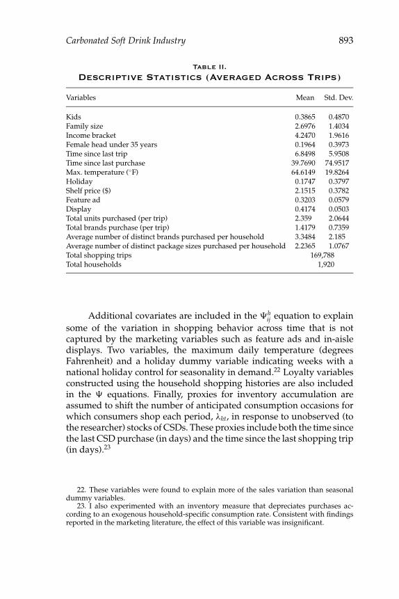
Descriptive Statistics (Averaged Across Trips)

Variables Mean Std. Dev.

Kids 0.3865 0.4870Family size 2.6976 1.4034Income bracket 4.2470 1.9616Female head under 35 years 0.1964 0.3973Time since last trip 6.8498 5.9508Time since last purchase 39.7690 74.9517Max. temperature (◦F) 64.6149 19.8264Holiday 0.1747 0.3797Shelf price ($) 2.1515 0.3782Feature ad 0.3203 0.0579Display 0.4174 0.0503Total units purchased (per trip) 2.359 2.0644Total brands purchase (per trip) 1.4179 0.7359Average number of distinct brands purchased per household 3.3484 2.185Average number of distinct package sizes purchased per household 2.2365 1.0767Total shopping trips 169,788Total households 1,920

Additional covariates are included in the �hij equation to explain

some of the variation in shopping behavior across time that is notcaptured by the marketing variables such as feature ads and in-aisledisplays. Two variables, the maximum daily temperature (degreesFahrenheit) and a holiday dummy variable indicating weeks with anational holiday control for seasonality in demand.22 Loyalty variablesconstructed using the household shopping histories are also includedin the � equations. Finally, proxies for inventory accumulation areassumed to shift the number of anticipated consumption occasions forwhich consumers shop each period, λht, in response to unobserved (tothe researcher) stocks of CSDs. These proxies include both the time sincethe last CSD purchase (in days) and the time since the last shopping trip(in days).23

22. These variables were found to explain more of the sales variation than seasonaldummy variables.

23. I also experimented with an inventory measure that depreciates purchases ac-cording to an exogenous household-specific consumption rate. Consistent with findingsreported in the marketing literature, the effect of this variable was insignificant.


Table III.

List of Products and their Characteristics(Ordered by Market Shares)

Product Sodium Carbs. Phos. Citric Caramel Clear

PEPSI CAN 12P 35 41 1 1 1 0COKE CAN 12P 50 39 1 0 1 0PEPSI CAN 6P 35 41 1 1 1 0COKE DIET CAN 12P 40 0 1 1 1 0PEPSI BOTTLE 67.6 oz 35 41 1 1 1 0PEPSI DIET CAN 12P 35 0 1 1 1 0COKE CAN 6P 50 39 1 0 1 0PEPSI DIET CAN 6P 35 0 1 1 1 0COKE BOTTLE 67.6 oz 50 39 1 0 1 0PEPSI DIET BOTTLE 67.6 oz 35 0 1 1 1 0COKE DIET CAN 6P 40 0 1 1 1 0DR PEPPER CAN 12P 55 40 1 0 1 0MOUNTAIN DEW CAN 12P 70 46 0 1 0 0DR PEPPER CAN 6P 55 40 1 0 1 07 UP CAFF-FREE BOTTLE 67.6 oz 75 39 0 1 0 1COKE DIET CAFF-FREE CAN 12P 40 0 1 1 1 0COKE DIET BOTTLE 67.6 oz 40 0 1 1 1 07 UP DIET CAFF-FREE BOTTLE 67.6 oz 35 0 0 1 0 1MOUNTAIN DEW CAN 6P 70 46 0 1 0 0SPRITE CAFF-FREE CAN 12P 70 38 0 1 0 1PEPSI DIET CAFF-FREE CAN 12P 35 0 1 1 1 0DR PEPPER BOTTLE 67.6 oz 55 40 1 0 1 0MOUNTAIN DEW BOTTLE 67.6 oz 70 46 0 1 0 0PEPSI BOTTLE 16 oz 35 41 1 1 1 0PEPSI DIET CAFF-FREE CAN 6P 35 0 1 1 1 0A & W CAFF-FREE CAN 6P 45 46 0 0 1 0

6. Results

6.1 Parameter Estimates

Estimation results are shown in Table IV, starting with the coefficientsof the quality function, �, in the first three columns. The abbreviation“s.d.” in a variable’s name indicates this is a standard deviation for arandom coefficient.24

The results imply that marketing variables such as feature ads anddisplays have a strong positive influence on purchasing behavior. How-ever, there is substantial heterogeneity in these responses as indicated bythe significant s.d. coefficients. Loyalty to the brand and to the specific

24. All standard errors have been corrected for potential serial dependence for up to15 days, which nearly doubles several of the standard errors.


Table IV.

Results of Demand Estimation

Perceived Quality � Nonlinear Terms, λ, α, m, γ

Variables Param SE Variables Param SE

Feature ad 0.796 0.025 λ: kids 0.0813 0.029S.d. feature ad 0.058 0.014 λ: family size 0.0418 0.0158Display 1.588 0.048 λ: time since last CSD 0.0003 0.0001S.d. display 0.204 0.027 λ: time since last trip −0.0047 0.0018Prod. loyalty 0.062 0.013 λ: temperature 0.0063 0.002Brand loyalty 0.015 0.220 λ: holiday −0.0015 0.0024Intercept −0.277 0.133 α: constant 5.0315 0.1556S.d. intercept 2.281 0.023 α: family size 0.6292 0.0334Diet −0.085 0.005 α: time since last CSD 0.0098 0.003S.d. diet 0.278 0.019 α: time since last trip 0.0145 0.0049Sodium −0.036 0.001 m: income 2.4484 0.0952Carbs 0.336 0.017 γ 0.0596 0.0021Caffeine 1.961 0.047Phos. −1.289 0.080Citric 0.070 0.027S.d. citric 0.240 0.031Caramel 1.539 0.030S.d. caramel 1.193 0.102Nocolor 2.202 0.062Cans ∗ 6 2.082 0.034S.d. cans ∗ 6 1.137 0.050Can ∗ 12 1.571 0.030S.d. cans ∗ 12 0.144 0.016Bottles ∗ 16 0.683 0.156S.d. bottles ∗ 16 2.049 0.224Kids ∗ caffeine 0.542 0.045(Family size) ∗ (pack size) 0.012 0.001(Female < 35) ∗ diet 0.329 0.033Hansen’s J statistic 184.48No. observations (trips) 169,788

product (UPC) chosen on the previous trip explain only a small portionof the perceived quality. The results suggest that loyalty to a specificbrand is stronger than loyalty to a given UPC.

As for demographic characteristics, I find that, as expected, house-holds with a female head under 35 years old tend to have higher pref-erences for diet products, a well-documented fact in the CSD industry.Larger households place slightly more weight on products with moreservings, such as the 12-pack of cans. Households with kids place ahigher weight on products with caffeine than without. This finding


could be due to the fact that the caffeine-free products, such as 7 UPand Sprite, tend to appeal more to adults.

The fourth to sixth columns of Table IV contain the estimatedcoefficients for the mean of the Poisson, λh, the marginal utility ofincome, αh, the vertical dimension of taste, mh, and the curvature of theutility function, γ . Beginning with λh, the expected number of decisionsa household makes on a given trip depends primarily on the presenceof kids and on family size. Temperature and holidays also increase thenumber of decisions. Proxies for inventory, time since last shopping tripand time since last CSD purchase, have small effects.

The marginal utility of income, αh, also increases with the numberof people in the household. Once again, the effects of time since last tripand time since last CSD purchase are very small. The vertical componentincreases with income, so that households with higher income perceivemore distance between products. Finally, the estimated values of γ arepositive and below 1, which is consistent with the notion that utility isconcave.25

6.2 Price Elasticities, Margins, and Marginal costs

Table V reports the aggregate price elasticities, marginal costs, and price-cost margins (PCM), p − c

p , corresponding to the aggregated quarterlyconsumer demand estimates. Marginal costs and PCMs are computedby assuming Nash equilibrium in manufacturer prices each quarter.The table reports the median level and standard error across the ninequarters in the sample.

Pepsi clearly has a pricing advantage over its rivals, setting mar-gins of about 50–60%. In comparison, Coke’s margins are around 40%.This fact is not surprising since Pepsi is the market leader in the Denvermarket. However, the relative pricing advantage of Pepsi in this marketwill likely have a downward bias on the welfare implications of the Cokeand Dr. Pepper mergers. 7 UP margins are also close to 40%, whereasDr. Pepper’s are closer to 30%. The marginal cost of a 67.6 ounce bottleis markedly lower than that of a 6-pack of cans, possibly reflecting therelative cost advantage of a plastic bottle versus an aluminum can. Thefact that 12-packs of cans have slightly higher marginal costs than 6-packs may reflect the more sophisticated cardboard box used to bundle12 cans, as opposed to the simple plastic ring used to bind the 6-packs.

25. I also calculate Hansen’s statistic to test our set of over-identifying restrictions. Iobtain a statistic of 184.48. Since we have 54 parameters and 160 moment conditions, thisstatistic is asymptotically distributed χ2 with 106 degrees of freedom. The critical value isroughly χ2

.05(106) = 124, and the model is rejected. In practice, this test is routinely rejectedwith large data sets and, hence, in our context it could be inconclusive.


Table V.

Own-Price Elasticities, Predicted Mark-Ups andMarginal Costs

Own-Price Elasticity MC ($/12 oz) PCM (%)Price ($/12 oz)

Product Median Median SE Median SE Median SE

PEPSI 12P 0.30 −3.36 0.15 0.14 0.03 51.5 1.66PEPSI 6P 0.27 −3.07 0.17 0.11 0.02 55.7 1.37PEPSI 67.6oz 0.18 −3.26 0.09 0.07 0.04 60.4 2.75PEPSI DT 12P 0.30 −3.06 0.29 0.11 0.03 63.9 2.15PEPSI DT 6P 0.26 −3.99 0.18 0.13 0.01 50.0 1.47PEPSI DT 67.6oz 0.18 −3.99 0.28 0.08 0.05 58.1 3.31PEPSI DT CF 12P 0.30 −5.00 0.62 0.15 0.04 47.5 2.77PEPSI DT CF 6P 0.26 −4.98 0.27 0.17 0.03 37.5 1.64PEPSI 16oz 0.33 −3.90 0.56 0.15 0.03 50.1 3.03MT DW 12P 0.30 −4.37 0.33 0.19 0.03 37.4 3.11MT DW 6P 0.27 −4.55 0.29 0.12 0.03 55.5 1.88MT DW 67.6oz 0.18 −3.79 0.19 0.09 0.04 50.3 2.30COKE CLS 12P 0.29 −3.64 0.18 0.17 0.06 43.3 3.66COKE CLS 6P 0.27 −4.05 0.25 0.18 0.02 33.9 1.27COKE CLS 67.6oz 0.19 −3.98 0.21 0.11 0.01 42.4 1.23COKE DT 12P 0.29 −3.67 0.21 0.15 0.15 47.5 10.30COKE DT 6P 0.27 −4.37 0.22 0.17 0.01 34.7 1.27COKE DT CF 12P 0.29 −5.62 1.17 0.19 0.01 32.2 1.21COKE DT 67.6oz 0.19 −4.04 0.18 0.11 0.06 42.3 4.48SP CF 12P 0.29 −3.86 0.23 0.17 0.04 44.6 2.357 UP R CF 67.6oz 0.18 −4.39 0.19 0.13 0.12 30.0 7.847 UP DT CF 67.6oz 0.18 −3.41 0.13 0.11 0.01 39.1 1.11DR PR 12P 0.31 −4.06 0.34 0.23 0.02 28.0 2.44DR PR 6P 0.28 −6.03 0.39 0.21 0.14 19.9 8.81DR PR 67.6oz 0.19 −3.89 0.23 0.13 0.11 30.3 8.54A and W CF 6P 0.28 −3.85 0.31 0.20 0.04 31.4 2.16

Standard errors were computed using a parametric bootstrap. 150 draws were taken from the asymptotic distributionof the parameters and used to compute a sample of MC, PCM and elasticities.

I find that Dr. Pepper has noticeably higher marginal costs than otherproducts. This result may reflect the differences in distribution costs.For instance, 7 UP has substantially lower costs than Dr. Pepper, but theformer is typically distributed via a Pepsi bottler since it is not consideredto be a direct competitor with the colas.

In Table VI, I report own and cross-price elasticities for a sampleof products (medians across the nine quarters).26 Interestingly, theelasticities demonstrate that consumers tend to substitute primarilybetween products of the same size in response to price changes. For

26. The complete set of elasticities is available in a separate appendix.


Table VI.

A Sample of Aggregate Own and Cross-PriceElasticities (Medians Across the 9 Quarters)

MT DR PEPSI COKEPEPSI COKE DW PR 7 UP DT DT PEPSI COKE

Product 12P 12P 12P 6P 67.6oz 12P 12P 6P 67.6oz

PEPSI 12P −3.10 0.39 0.77 0.18 0.31 0.48 0.41 0.13 0.46PEPSI 6P 0.15 0.12 0.15 0.80 0.42 0.05 0.16 −3.25 0.36PEPSI 67.6oz 0.21 0.14 0.21 0.24 0.44 0.17 0.13 0.15 0.53PEPSI DT 12P 0.53 0.30 0.45 0.20 0.24 −3.43 0.21 0.07 0.11PEPSI DT 6P 0.08 0.15 0.01 0.61 0.15 0.07 0.15 0.55 0.07PEPSI DT 67.6oz 0.06 0.05 0.05 0.05 0.24 0.11 0.05 0.05 0.20PEPSI DT CF 12P 0.03 0.03 0.00 0.00 0.03 0.10 0.01 0.00 0.06PEPSI DT CF 6P 0.02 0.01 0.04 0.63 0.02 0.02 0.02 0.02 0.04PEPSI 16oz 0.07 0.05 0.12 0.00 0.16 0.04 0.11 0.08 0.11MT DW 12P 0.08 0.14 −4.42 0.00 0.05 0.08 0.01 0.02 0.04MT DW 6P 0.00 0.03 0.07 0.08 0.11 0.00 0.12 0.26 0.01MT DW 67.6oz 0.05 0.04 0.08 0.12 0.17 0.02 0.03 0.04 0.12COKE 12P 0.34 −3.52 0.50 0.24 0.25 0.45 1.15 0.16 0.18COKE 6P 0.12 0.11 0.23 0.86 0.20 0.20 0.08 0.46 0.16COKE 67.6oz 0.06 0.06 0.03 0.22 0.30 0.08 0.21 0.09 −3.89COKE DT 12P 0.11 0.55 0.21 0.10 0.16 0.29 −3.96 0.03 0.36COKE DT 6P 0.11 0.03 0.02 0.27 0.11 0.05 0.05 0.28 0.10COKE DT CF 12P 0.02 0.06 0.07 0.06 0.02 0.08 0.08 0.00 0.03COKE DT 67.6oz 0.05 0.11 0.04 0.02 0.27 0.08 0.05 0.05 0.81SP CF 12P 0.07 0.17 0.18 0.09 0.11 0.07 0.09 0.06 0.057 UP CF 67.6oz 0.08 0.06 0.10 0.01 −4.25 0.08 0.07 0.07 0.127 UP DT CF 67.6oz 0.05 0.08 0.17 0.12 0.95 0.01 0.08 0.05 0.15DR PR 12P 0.26 0.29 0.17 0.11 0.20 0.32 0.10 0.04 0.09DR PR 6P 0.01 0.01 0.02 −5.76 0.02 0.01 0.04 0.09 0.09DR PR 67.6oz 0.06 0.05 0.06 0.09 0.16 0.04 0.04 0.10 0.26A & W CF 6P 0.05 0.02 0.02 0.23 0.07 0.04 0.04 0.13 0.03

instance, demand for 6-packs of Diet Pepsi are quite sensitive to the priceof 6-packs of Pepsi, and demand for 67.6 oz bottles of 7 UP are sensitiveto the price of 67.6 oz bottles of Diet 7 UP. This finding is consistent withour discussion of typical shopping baskets, in the data section above. Inaddition, Coke and Pepsi are clearly the primary substitutes of almostevery brand, but the reverse is not true. Although not reported, I findthat a random coefficients logit model estimated using household dataprovides substantially lower own and cross-price elasticities. The logitdemand system is a more traditional approach to analyzing mergersthat ignores multiple discreteness.

In a separate appendix, I conduct several sensitivity checks of theresults to alternative controls for consumer heterogeneity. The findings


indicate that fewer controls for unobserved heterogeneity in tastes leadsto more inelastic demand estimates. I also find that the use of alternativespecifications to control for state dependence in consumer tastes (i.e.,loyalty) does not seem to have much impact on the price elasticitiesof demand. I also find my results to be fairly robust to the scope ofproducts used. Increasing the product set to include the top 30 UPCsdoes not change the elasticity estimates, while decreasing the set to thetop 20 does lead to more inelastic demand estimates.27

6.3 Mergers

In this section, I use my results to simulate the equilibrium prices andquantities for the proposed 1986 mergers between Coke and Dr. Pepper,and Pepsi and 7 UP as well as the hypothetical merger between Cokeand Pepsi.28 In evaluating the mergers, I assume that the large sunk costsassociated with a new brand are prohibitively high to expect entry, evenif a merger raises overall prices. These sunk costs consist of advertisingoutlays for launching new brands as well as slotting fees to retailersto obtain shelf space even for new package sizes of existing brands(Israilevich, 2003). In addition, I assume that a merger only affects thepricing decisions of firms (i.e., internalizes pricing of both merged firms’product lines) and, hence, consumer demand is only affected insofar asconsumers face different prices. Hence, the definition of loyalty andother purchase-related variables do not change post-merger.

Table VII reports the median predicted quarterly price changes,in percent, for each merger across the nine quarters in the sample.29

The first column reports the changes in prices associated with breakingapart Dr. Pepper and 7 UP, to replicate the 1986 market structure. Thisbreak-up appears to have had a very small impact on industry prices.From an economic standpoint, the change in prices associated witha merger does not capture the impact on the well-being of economicagents: consumers and producers. As in Werden and Froeb (1994) andNevo (2000), Table VIII reports the corresponding changes in producerand consumer surplus for each merger. Producer surplus correspondsto variable profits and consumer surplus corresponds to the Hicksiancompensating variation. The sample predictions are aggregated to themarket level using a projection factor reported by AC Nielsen. Hence,

27. The results from these analyses and the appendix can be found on my website at:http://gsbwww.uchicago.edu/fac/jean-pierre.dube/research/.

28. Although the relevant set of brands has not changed since the time of the trial, in1989, Dr. Pepper and 7 UP were both acquired by Hicks and Haas.

29. The approximation of Hausman et al. (1994), holding elasticities constant, tends tooverstate the price increases compared to those computed numerically.


Table VII.

Median Simulated Percent Change in QuarterlyPrice from Mergers

Product 1986 Coke/Dr. Pepper Pepsi/7 UP Coke/Pepsi

PEPSI 12P 0.03 0.10 0.82 12.25PEPSI 6P 0.01 0.11 0.55 19.19PEPSI 67.6oz −0.11 0.32 2.18 13.10PEPSI DT 12P 0.09 −0.05 0.99 23.75PEPSI DT 6P 0.04 −0.27 0.22 14.28PEPSI DT 67.6oz −0.04 0.19 1.53 16.84PEPSI DT CF 12P 0.83 −1.12 −1.66 21.01PEPSI DT CF 6P 1.27 −1.41 −1.37 19.25PEPSI 16oz 0.06 −0.40 0.19 12.32MT DW 12P 0.24 −0.90 0.08 18.49MT DW 6P 0.33 −0.57 0.17 14.81MT DW 67.6oz 0.03 −0.16 2.16 12.67COKE CLS 12P 0.04 1.03 0.05 16.00COKE CLS 6P 0.04 1.65 −0.14 20.95COKE CLS 67.6oz −0.09 2.16 0.46 24.94COKE DT 12P 0.14 1.06 −0.05 21.42COKE DT 6P 0.08 0.62 −0.48 21.99COKE DT CF 12P 1.25 0.24 −1.93 15.33COKE DT 67.6oz 0.09 0.68 0.12 20.93SP CF 12P 0.24 −0.74 −4.89 7.827 UP R CF 67.6oz −1.70 0.99 16.56 10.477 UP DT CF 67.6oz −1.54 −0.12 14.15 11.44DR PR 12P −0.78 5.75 −0.30 7.07DR PR 6P −0.84 3.60 0.34 5.88DR PR 67.6oz −1.10 4.64 −0.02 9.39A and W CF 6P −1.26 −1.14 0.49 9.20

the merger simulations should be interpreted as applying to the entireDenver scantrac.

The first merger, between Coke and Dr. Pepper, did not seem tohave a large effect on prices. Coke prices never rise by more than about2% and the prices of Dr. Pepper increase by between 4% and 6%. Despitethe seemingly moderate price increases, the merger had substantialimplications for welfare. Interestingly, the rise in prices appeared tohave a large benefit for Pepsi and 7 UP, whose quarterly variable profitsrose by $261,000 and $9,000, respectively (about 3% in both cases).The total joint quarterly profitability of Coke and Dr. Pepper increasedonly slightly, just under 1% on average. The increased profitabilityof Coke products was generated by the less profitable pricing of Dr.Pepper products. The reduced profitability of Dr. Pepper products couldbe understated because the analysis does not take into account thepotential cost advantages from leveraging Coca-Cola distribution.


Table VIII.

Median change in Quarterly Welfare (Thousandsof Dollars Per Quarter)

Coke/Dr. Pepper Pepsi/7 UP Coke/Pepsi

Pepsi 261.41 168.62 567.02Coke 60.65 203.01 133.17Dr. Pepper −41.88 36.31 179.217 UP 9.28 −44.39 100.35Consumers −1291.42 −1901.36 −29707.28Total −998.24 −1533.51 −28727.53

Quarterly consumer surplus fell, on average, by $1.2 million. Despite thegains in profits, aggregate welfare in the Denver economy fell overall byalmost $1 million. Aggregating up to the entire US economy, (approxi-mated by the 50 largest Nielsen scantracs), implied welfare losses of atleast $50 million per quarter. In addition, because Denver is a mid-sizedNielsen scantrac and because Denver is a Pepsi-dominated market, thetotal US welfare losses could be even larger. These substantial losseswarranted the efforts of the FTC, not only to block the merger in 1986, butto limit Coca-Cola’s ability to acquire large competitors for the decadeafter 1994.

For the merger between Pepsi and 7 UP, cola prices did not riseby much more than 2%. However, the price of 7 UP rises between 14%and 16%. The joint profits of 7 UP and Pepsi rose by about 1.5%, mainlybecause increasing 7 UP product prices improved the profitability ofPepsi products. Profits also rise at both Coke and Dr. Pepper by 6%and 9%, respectively. At the same time, consumer surplus fell by almost$2 million. Overall, the merger led to roughly $1.5 million in lost surplusfor the Denver market in each quarter. These much more dramatic priceincreases and welfare losses, at the expense of consumer well-being,likely explain why Pepsi did not fight the FTC’s decision to contest themerger.

In the final column, I consider the extreme case of a merger betweenCoke and Pepsi, which Coke insisted would be the only merger ofanticompetitive consequence. I now find substantial price increases, asexpected. With the exception of Sprite, all of Pepsi and Coke’s products’prices increased by well over 10%. In fact, many rose by more than 20%,especially the diet colas. This drastic reduction in cola competition hadthe indirect effect of allowing 7 UP, Dr. Pepper, and A & W Rootbeer eachto raise their prices substantially. The large increase in prices resulted inabout a $700,000 average increase in the quarterly joint variable profitsof Coke and Pepsi, roughly an 8% improvement. These gains came at a


huge cost to consumers, who lost an average of $30 million in quarterlyconsumer surplus. Overall, the Denver economy suffered an almost$29 million loss in aggregate surplus, on average.

This analysis is limited by the static nature of the model of produc-ers. Hence, the analysis does not consider the possibility that postmergerprofit gains could stimulate entry of new firms into the market. More-over, the analysis does not account for potential efficiency gains fromjoint production of merged firms. During the 1986 trial, Coke argued thatDr. Pepper would benefit from increased production efficiency and scaleeconomies in distribution, both of which would lower production costssubstantially. However, little evidence was provided to quantify theseefficiency gains. In the case of Pepsi and 7 UP, 7 UP already piggybacksoff Pepsi’s bottling and distribution network in most markets. Thus, anypotential efficiency gains for 7 UP would need to reflect the productionof concentrated syrup.

7. Conclusions

Recent advances in the collection of checkout scanner data have helpedbring newer and more sophisticated structural econometric tools intomerger analysis. Existing methods have relied on simplifying assump-tions, such as discrete choice purchase behavior, to help build parsimo-nious demand systems for these analyses. However, in industries suchas CSDs, the single unit purchase assumption is inappropriate. I resolvethis problem by using disaggregate household-level point-of-purchasedata to estimate demand. These microdata provides information on thevariation in assortments purchased across households and shoppingtrips. The Hendel (1999) specification is used to model demand for theseassortments. These demand estimates are then aggregated to simulatethe impact of several hypothetical CSD mergers. Lacking comparabledata and modeling techniques, the FTC was unable to conduct thesetypes of merger simulations to evaluate the proposed acquisition of Dr.Pepper by Coca-Cola Co back in 1986. Despite the moderate impacton prices of the merger between Coca-Cola Co. and Dr. Pepper, Ifind evidence of fairly large welfare losses. The price implications andwelfare losses are even more substantial for the merger of PepsiCo. and7 UP and, especially, for the hypothetical merger of Coca-Cola Co. andPepsiCo.

The current work has some limitations. The treatment of unob-served heterogeneity pertains to the randomness of tastes across thelatent consumption occasions. The random coefficients do not capturepersistent household-specific unobserved tastes. To capture persistentsources of household-specific heterogeneity, I use a rich set of de-mographic information, which I interact with several aspects of the


model. Nonetheless, I find some evidence of serial dependence in theunexplained portion of the model. Although this dependence couldsimply reflect sampling problems, it could also come from unmeasuredheterogeneity. Unmeasured heterogeneity could bias the estimates ofloyalty. To check this problem, I reestimate the model without the loyaltyparameters and find little effect on the estimated elasticities, increasingmy confidence that the current results are not biased. I also find myresults to be robust across several different specifications of loyalty.

The current work is also based entirely on static modeling assump-tions. Potential sources for future research include studying variousforms of consumer dynamics insofar as they influence assortment deci-sions. For instance, expectations of short-run price fluctuations, such asfuture sales, could cause consumers to defer purchases until the time ofthe sale. One might expect consumers to “stock-up” during sale periods,purchasing large assortments of items while they are perceived to bea good deal (Erdem et al., 2003). Alternatively, as consumers becomeexperienced with certain goods, they may begin to vary their purchaseassortment to seek variety. On the supply side, the study of equilibriumpricing could be extended to include the timing of short-run price cutsand, subsequently, the impact of mergers on these types of consumer-driven promotions.

References

Baker, J.B. and T.F. Bresnahan, 1985, “The Gains from Merger or Collusion in Product-Differentiated Industries,” The Journal of Industrial Economics, 33, 427–444.

Bell, D.R., J. Chiang, and V. Padmanabhan, 1999, “The Decomposition of PromotionalResponse: An Empirical Generalization,” Marketing Science, 18, 504–526.

Berry, S., 1994, “Estimating Discrete-Choice Models of Product Differentiation,” RandJournal of Economics, 25, 242–262.

—— and A. Pakes, 1993, “Some Applications and Limitations of Recent Advances inEmpirical Industrial Organization: Merger Analysis,” American Economic Review, 83,247–252.

Berto Villas–Boas, S., 2001, “Vertical Contracts Between Manufacturers and Re-tailers: Inference with Limited Data,” Working Paper, University of California,Berkeley.

Bresnahan, T.F., 1989, “Empirical Methods for Industries with Market Power,” in R.Schmalensee and R. Willig, eds. Handbook of Industrial Organization, Amsterdam, NorthHolland: Elsevier Science.

Chintagunta, P., 1993, “Investigating Purchase Incidence, Brand Choice and PurchaseQuantity Decisions of Households,” Marketing Science, 12, 184–208.

Cotterill, R.W., A.W. Franklin, and L.Y. Ma, 1996, “Measuring Market Power Effects inDifferentiated Product Industries: An Application to the Soft Drink Industry,” FoodMarketing Policy Center, University of Connecticut, Storrs, CT.

Dube, J.P., 2004, “Multiple Discreteness and Product Differentiation: Demand for Carbon-ated Soft Drinks,” Marketing Science, 23(1).

Erdem, T., 1996, “A Dynamic Analysis of Market Structure Based on Panel Data,” MarketingScience, 15, 359–378.


——, S. Imai, and M.P. Keane, 2003, “A Model of Consumer Brand and Quantity ChoiceDynamics Under Price Uncertainty,” Quantitative Marketing and Economics, 1(1), 5–64.

Gasmi, F., J.J. Laffont, and Q. Vuong, 1992, “Econometric Analysis of Collusive Behaviorin a Soft-Drink Market,” Journal of Economics and Management Strategy, 1, 277–311.

Guadagni, P.M. and J.D.C. Little, 1983, “A Logit Model of Brand Choice Calibrated onScanner Data,” Marketing Science, 2, 203–238.

Hansen, L.P., 1982, “Large Sample Properties of Generalized Method of Moments Estima-tors,” Econometrica, 50, 1092–1054.

Hauser, J.R. and B. Wernerfelt, 1990, “An Evaluation Cost Model of Consideration Sets,”Journal of Consumer Research, 16, 393–408.

Hausman, J. A., G.K. Leonard, and D. McFadden, 1995, “A Utility-Consistent, CombinedDiscrete Choice and Count Data Model: Assessing Recreational Use Losses due toNatural Resource Damage,” Journal of Public Economics, 56, 1–30.

——, ——, and J.D. Zona, 1994, “Competitive Analysis with Differenciated Products,”Annales d’Economie et de Statistique, 34, 159–180.

Hendel, I., 1999, “Estimating Multiple-Discrete Choice Models: An Application to Com-puterization Returns,” Review of Economic Studies, 66, 423–446.

Israilevich, G., 2004, “Assessing Supermarket Product-Line Decisions: The Impact ofSlotting Fees,” Quantitative Marketing and Economics, 2, 141–167.

Keane, M.P., 1997, “Modeling Heterogeneity and State Dependence in Consumer ChoiceBehavior,” Journal of Business and Economic Statistics, 15, 310–327.

Kim, J., G.M. Allenby, and P.E. Rossi, 2002, “Modeling Consumer Demand for Variety,”Marketing Science, 21, 229–250.

Langan, G.E. and R.W. Cotterill, 1994, “Estimating Brand Level Demand Elasticitiesand Measuring Market Power for Regular Carbonated Soft Drinks,” University ofConnecticut, Storrs, CT.

McFadden, D., 1989, “A Method of Simulated Moments for Estimation of DiscreteResponse Models Without Numerical Integration,” Econometrica, 57, 995–1026.

Muris, T.J., D.T. Scheffman, and P.T. Spiller, 1992, “Strategy and Transaction Costs:The Organization of Distribution in the Carbonated Soft Drink Industry,” Journal ofEconomics and Management Strategy, 1, 83–128.

Newey, W.K. and K.D. West, 1987, “A Simple, Positive Semi-Definite, Hetroskedasticityand Autocorrelation Consistent Covariance Matrix,” Econometrica, 55, 703–708.

Nevo, A., 2000, “Mergers with Differentiated Products: The Case of the Ready-to-EatCereal Industry,” The Rand Journal of Economics, 31, 395–421.

Pakes, A. and D. Pollard, 1989, “Simulation and the Asymptotics of Optimization Estima-tors,” Econometrica, 57, 1027–1057.

Shum, M., 2000, “Does Advertising Overcome Brand Loyalty? Evidence from the BreakfastCereals Market,” Johns Hopkins University, Working Paper.

Slade, M.E., 1995, “Product Market Rivalry with Multiple Strategic Weapons: An Analysisof Price and Advertising Competition,” Journal of Economics and Management Strategy,4, 445–476.

Villas-Boas, M. and R. Winer, 1999, “Endogeneity in Brand Choice Models,” ManagementScience, 45(10), 1324–1338.

Walsh, J.W., 1995, “Flexibility in Consumer Purchasing for Uncertain Future Tastes,”Marketing Science, 14, 148–165.

Werden, G.J. and L.M. Froeb, 1994, “The Effects of Mergers in Differentiated Products In-dustries: Logit Demand and Merger Policy,” Journal of Law, Economics and Organization,10, 407–426.

White, L.J., 1989, “The Proposed Merger of Coca-Cola and Dr Pepper,” in J.E. Kwoka andL.J. White, eds., The Antitrust Revolution, Glenview, Ill: Scott, Foresman, pp 76–95.

Documents

Product Differentiation and Mergers in the Carbonated Soft ...€¦ · the Carbonated Soft Drink Industry ... Oxford OX4 2DQ, UK. Journal of Economics & Management Strategy, Volume