Problem solving using process algebraconsidered insightful

J.F. Groote (3-2196-6587) and E.P. de Vink (1-9514-2260)

Department of Mathematics and Computer Science,Eindhoven University of Technology, Eindhoven, The Netherlands

J.F.Groote@tue.nl, E.P.d.Vink@tue.nl

Abstract. Process algebras with data, such as LOTOS, PSF, FDR, andmCRL2, are very suitable to model and analyse combinatorial problems.Contrary to more traditional mathematics, many of these problems can verydirectly be formulated in process algebra. Using a wide range of techniques,such as behavioural reductions, model checking, and visualisation, the prob-lems can subsequently be easily solved. With the advent of probabilisticprocess algebras this also extends to problems where probabilities play arole. In this paper we model and analyse a number of very well-known – yettricky – problems and show the elegance of behavioural analysis.

1 Introduction

There is great joy in solving combinatorial puzzles. Numerous books have ap-peared describing those [13,33]. And although some of the puzzles are easy tosolve once properly understood, they are real brain teasers for most people.

Many of these puzzles are about behaviour. Classical mathematics and logichardly provides an effective context to solve such problems systematically. Thisis apparent if one considers classical analysis. But also fields like graph theory,combinatorics, combinatorial optimisation, probability theory, and even logic allrequire a translation of the problem to the mathematical domain that is generallynot completely straightforward.

This is where process algebras come in. Process algebras are very suited todescribe the behaviour often present in the puzzles mentioned. In the last decadesnumerous tools have been developed to provide insight in the behaviour denotedin a process algebra expression as it quickly became clear that the behaviourdescribed in such an expression can be rather intricate. This gave rise to hidingof actions, behavioural reductions, various visualisation techniques, as well asmodal logics to express and validate properties about behaviour.

The early 1970s can be seen as the period when process algebra was born.Both Milner and Bekic wrote a treatise expressing that actions were importantto study behaviour [2,25,27]. It was the seminal work of Milner in 1981 that putprocess algebras on the map [28]. This had quite some effect. For instance Hoarepresented CSP in 1978 as an advanced programming language [21], whereas he

presented it in 1985 as a process algebra [22]. The work on CSP has been devel-oped into the impressive family of tools, FDR, that are based on failure divergencerefinement [31,14].

The work on CCS also inspired the design of the language LOTOS [24] as alanguage to model communication services and protocols. A major role in its de-velopment was played by the Technische Hogeschool Twente (now Twente Univer-sity) first in the completely formal standardisation of the language, with Brinksmaas main editor, and later in activities to build tools around it. Notable are theextensive formal specifications of standard protocols, but also those of manufac-turing systems, that were developed at the time [5,7,32]. The CADP toolset stemsfrom this period [12]. It is the only major toolset still capable of analysing LOTOSspecifications. Furthermore, it has become quite powerful throughout the years.

The Algebra of Communicating Processes (ACP) was developed in Amster-dam [3,4] around the same time. In order to model practical systems first PSF(Protocol Specification Formalism) was designed [26], which was followed by thesimpler formalism µCRL [18], later renamed to mCRL2, which was also directedtowards analysis of practical specifications [17]. All these LOTOS-like formalismsuse data based on abstract equational datatypes. mCRL2 also supports time andthese days also probabilities.

An important feature of mCRL2 is the support for a modal logic with time anddata, which is very useful to investigate properties of the described behaviour.Temporal logic, with the operators [F] and [P], stems from [30]. Pnueli pointedto the applicability of formal logics to analyse behaviour [29]. For mCRL2 weare using the modal mu-calculus which is essentially Hennessy-Milner logic [20]with fixed points [23]. An alternative is the use of linear time logic (LTL [29])or computational tree logic (CTL [8]), but these are far less expressive than themodal mu-calculus [15].

In this paper we show process algebraic models of a number of well-known math-ematical puzzles. Most people find them hard to solve when they are confrontedwith them for the first time. We show that the puzzles can straightforwardly bemodelled into process algebra and using the standard analysis tools, such as be-havioural reduction, model checking, and visualisation, the solutions to these puz-zles are easy to obtain.

The major observation is that process algebra is an industrious mathematicaldiscipline in itself due to its capacity to understand worldly phenomena. Tradi-tionally, there is a tendency to think that process algebras, or more generallyformal methods, are intended to analyse software, protocols, and complex dis-tributed algorithms. But the application to examples as in this paper shows thatprocess algebra has an independent stand.

In this paper we use the language mCRL2, as we are acquainted with it,and it offers all we need, namely the capacity to express behaviour, data struc-tures, probabilities, time (although we do not exploit time here), and modal for-mulas. mCRL2 has a very rich toolset offering a whole range of analysis methods,far more than we use for the examples in this article. In the following we do

2

not explain the tool nor the formalism. For this we refer to [17] or the webpagewww.mcrl2.org. The examples in this article are part of the mCRL2 distributiondownloadable from this website.

2 The problem of the wolf, goat, and cabbage

A problem that is well-known, at least to the people in Western Europe, is theproblem of the wolf, the goat, and the cabbage: A traveller walks through stretchedRussian woods together with a friendly wolf, a goat, and a cabbage. Hungry andworn out, this companionship arrives at a river that they must cross. There is asmall boat only sufficient to carry our traveller and either the wolf, the goat, or thecabbage. More than two do not fit. Crossing is complex as when left unsupervisedby the traveller, the wolf will eat the goat, while the goat will eat the cabbage. Thequestion to answer is whether it is possible to cross the river without the goat orthe cabbage being eaten.

This problem is quite old. It already appeared in a manuscript from the eighthcentury A.D. [1]. Dijkstra wrote one of his well-known EWDs addressing thisproblem [10]. The description in mCRL2 can be found in Table 1. The descrip-tion uses two shores, left and right, which are essentially sets of ‘items’, i.e. setsof wolf, goat, and/or cabbage, resting at that shore. The opposite shore is given bya function opp. An update function is used to remove items from one side and addit to the other.

The behaviour of crossing the river is given by the process WGC. It has twoparameters, namely the shores s comprised of the sets of items at each side of theriver, and the current position p of the traveller. Observe that mCRL2 accommo-dates the use of data types such as sets which allows to neatly describe the shoresas a pair of sets containing items. The first two pairs of lines of the WGC processexpress that if the wolf and the goat, or the goat and the cabbage are at the sideopposite of the traveller, something is eaten, expressed by the action is_eaten.The symbol δ indicates that the process stops after this action. Note that actionsare typeset in a different font for easy recognition.

The third group of lines of the process expresses that the traveller can moveto the other shore alone, by performing the move action. To reduce the number oftransitions somewhat, we only allow this when no item can be eaten. The fourthgroup of lines expresses that the traveller can transport one item from one shoreto the other. The last group of lines states that if the complete companionshiparrives at the right shore, the action done can take place. Initially, the traveller,wolf, goat, and cabbage are at the left shore.

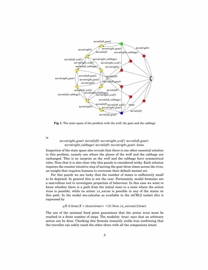
As the state space of this behaviour is small, it can nicely be visualised. SeeFigure 1. At the top we find the initial state, which is green. The goal state iscoloured blue at the bottom. All states where an action is_eaten can be doneare coloured red. They go to the white deadlocked state. All labels is_eaten areremoved for readability. States where nothing is eaten are green, yellow, or blue.It is easy to see that there are paths from the green to the blue state throughyellow states by moving counter clock wise through the graph. One of such paths

3

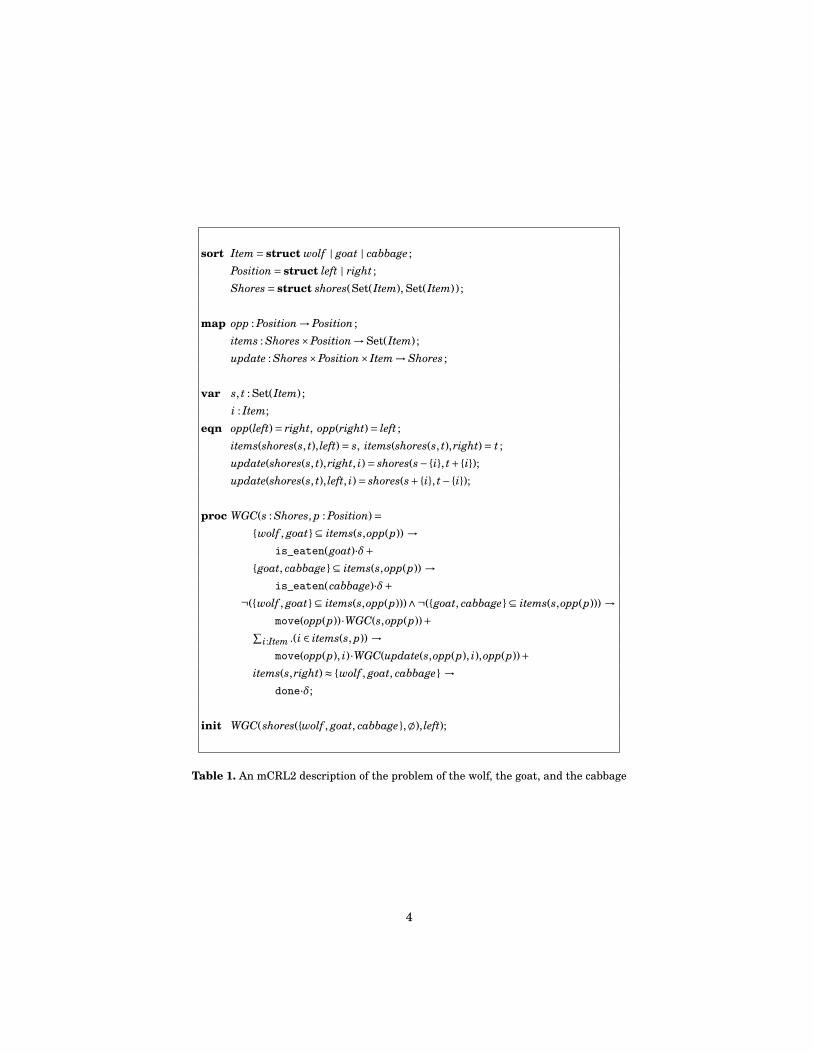
sort Item= struct wolf | goat | cabbage ;Position= struct left | right ;Shores= struct shores(Set(Item), Set(Item) ) ;

map opp : Position→Position ;items : Shores×Position→Set(Item) ;update : Shores×Position× Item→Shores ;

var s, t : Set(Item) ;i : Item;

eqn opp(left)= right, opp(right)= left ;items(shores(s, t), left)= s, items(shores(s, t),right)= t ;update(shores(s, t),right, i)= shores(s− {i}, t+ {i});update(shores(s, t), left, i)= shores(s+ {i}, t− {i});

proc WGC(s : Shores, p : Position)={wolf , goat }⊆ items(s,opp(p)) →

is_eaten(goat)·δ+{goat, cabbage }⊆ items(s,opp(p)) →

is_eaten(cabbage)·δ+¬({wolf , goat }⊆ items(s,opp(p)))∧¬({goat, cabbage }⊆ items(s,opp(p))) →

move(opp(p))·WGC(s,opp(p))+∑i:Item .(i ∈ items(s, p)) →

move(opp(p), i)·WGC(update(s,opp(p), i),opp(p))+items(s,right)≈ {wolf , goat, cabbage } →

done·δ;

init WGC(shores({wolf , goat, cabbage },;), left);

Table 1. An mCRL2 description of the problem of the wolf, the goat, and the cabbage

4

move(right,wolf )

move(right,goat)move(right,cabbage)

move(right)

move(left,goat)

move(left)

move(right,wolf )move(right,cabbage)

move(right)

move(left,wolf )

move(left,goat) move(left)

move(left,goat)

move(left,cabbage)

move(left)

move(right,goat)

move(right,cabbage)

move(right)

move(right,wolf )

move(right,goat)

move(right)

move(left,wolf )

move(left,cabbage)

move(left)move(right,goat)move(right)

donemove(left,wolf )

move(left,goat)

move(left,cabbage)

move(left)

Fig. 1. The state space of the problem with the wolf, the goat and the cabbage

ismove(right,goat) ·move(left) ·move(right,wolf ) ·move(left,goat) ·

move(right,cabbage) ·move(left) ·move(right,goat) ·done.

Inspection of the state space also reveals that there is one other essential solutionto this problem, namely one where the places of the wolf and the cabbage areexchanged. This is no surprise as the wolf and the cabbage have symmetricalroles. Note that it is also clear why this puzzle is considered tricky. Each solutionrequires the counter intuitive step of moving the goat three times across the river,an insight that requires humans to overcome their default mental set.

For this puzzle we are lucky that the number of states is sufficiently smallto be depicted. In general this is not the case. Fortunately, modal formulas area marvellous tool to investigate properties of behaviour. In this case we want toknow whether there is a path from the initial state to a state where the actiondone is possible, while no action is_eaten is possible in any of the states onthis path. In the modal mu-calculus as available in the mCRL2 toolset this isexpressed by

µX .((⟨true⟩X ∨⟨done⟩true)∧¬⟨∃i: Item.is_eaten(i)⟩true).

The use of the minimal fixed point guarantees that the action done must bereached in a finite number of steps. The modality ⟨true⟩ says that an arbitraryaction can be done. Checking this formula instantly yields true confirming thatthe traveller can safely reach the other shore with all the companions intact.

5

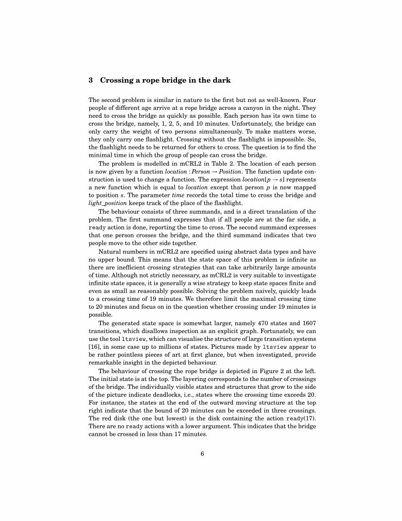
3 Crossing a rope bridge in the dark

The second problem is similar in nature to the first but not as well-known. Fourpeople of different age arrive at a rope bridge across a canyon in the night. Theyneed to cross the bridge as quickly as possible. Each person has its own time tocross the bridge, namely, 1, 2, 5, and 10 minutes. Unfortunately, the bridge canonly carry the weight of two persons simultaneously. To make matters worse,they only carry one flashlight. Crossing without the flashlight is impossible. So,the flashlight needs to be returned for others to cross. The question is to find theminimal time in which the group of people can cross the bridge.

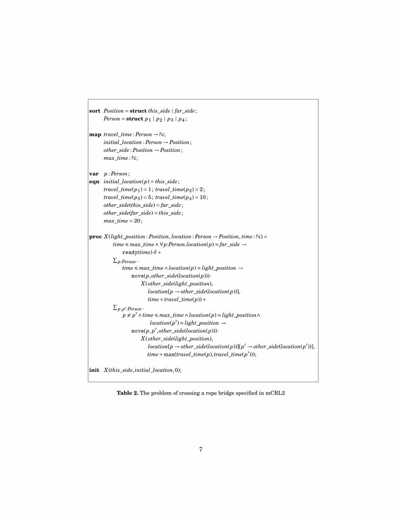
The problem is modelled in mCRL2 in Table 2. The location of each personis now given by a function location : Person → Position. The function update con-struction is used to change a function. The expression location[p → s] representsa new function which is equal to location except that person p is now mappedto position s. The parameter time records the total time to cross the bridge andlight_position keeps track of the place of the flashlight.

The behaviour consists of three summands, and is a direct translation of theproblem. The first summand expresses that if all people are at the far side, aready action is done, reporting the time to cross. The second summand expressesthat one person crosses the bridge, and the third summand indicates that twopeople move to the other side together.

Natural numbers in mCRL2 are specified using abstract data types and haveno upper bound. This means that the state space of this problem is infinite asthere are inefficient crossing strategies that can take arbitrarily large amountsof time. Although not strictly necessary, as mCRL2 is very suitable to investigateinfinite state spaces, it is generally a wise strategy to keep state spaces finite andeven as small as reasonably possible. Solving the problem naively, quickly leadsto a crossing time of 19 minutes. We therefore limit the maximal crossing timeto 20 minutes and focus on in the question whether crossing under 19 minutes ispossible.

The generated state space is somewhat larger, namely 470 states and 1607transitions, which disallows inspection as an explicit graph. Fortunately, we canuse the tool ltsview, which can visualise the structure of large transition systems[16], in some case up to millions of states. Pictures made by ltsview appear tobe rather pointless pieces of art at first glance, but when investigated, provideremarkable insight in the depicted behaviour.

The behaviour of crossing the rope bridge is depicted in Figure 2 at the left.The initial state is at the top. The layering corresponds to the number of crossingsof the bridge. The individually visible states and structures that grow to the sideof the picture indicate deadlocks, i.e., states where the crossing time exceeds 20.For instance, the states at the end of the outward moving structure at the topright indicate that the bound of 20 minutes can be exceeded in three crossings.The red disk (the one but lowest) is the disk containing the action ready(17).There are no ready actions with a lower argument. This indicates that the bridgecannot be crossed in less than 17 minutes.

6

sort Position= struct this_side | far_side ;Person= struct p1 | p2 | p3 | p4 ;

map travel_time : Person→N ;initial_location : Person→Position ;other_side : Position→Position ;max_time :N ;

var p : Person ;eqn initial_location(p)= this_side ;

travel_time(p1)= 1; travel_time(p2)= 2;travel_time(p3)= 5; travel_time(p4)= 10;other_side(this_side)= far_side ;other_side(far_side)= this_side ;max_time= 20;

proc X ( light_position : Position, location : Person→Position, time :N )=timeÉmax_time∧∀p:Person.location(p)≈ far_side →

ready(time)·δ+∑p:Person .

timeÉmax_time∧ location(p)≈ light_position →move(p,other_side(location(p))) ·

X (other_side(light_position),location[p → other_side(location(p))],time+ travel_time(p))+∑

p,p′:Person .p 6≈ p′∧ timeÉmax_time∧ location(p)≈ light_position∧

location(p′)≈ light_position →move(p, p′,other_side(location(p))) ·

X (other_side(light_position),location[p → other_side(location(p))][p′ → other_side(location(p′))],time+max(travel_time(p), travel_time(p′)));

init X (this_side, initial_location,0);

Table 2. The problem of crossing a rope bridge specified in mCRL2

7

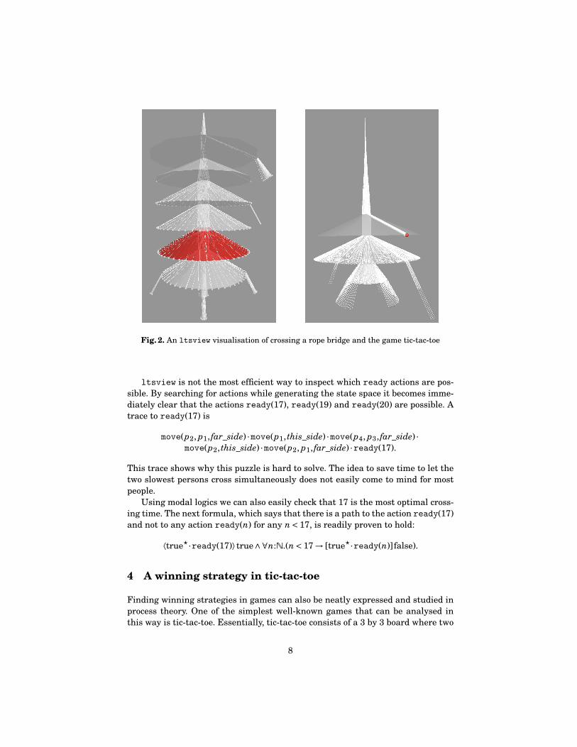
Fig. 2. An ltsview visualisation of crossing a rope bridge and the game tic-tac-toe

ltsview is not the most efficient way to inspect which ready actions are pos-sible. By searching for actions while generating the state space it becomes imme-diately clear that the actions ready(17), ready(19) and ready(20) are possible. Atrace to ready(17) is

move(p2, p1, far_side) ·move(p1,this_side) ·move(p4, p3, far_side) ·move(p2,this_side) ·move(p2, p1, far_side) ·ready(17).

This trace shows why this puzzle is hard to solve. The idea to save time to let thetwo slowest persons cross simultaneously does not easily come to mind for mostpeople.

Using modal logics we can also easily check that 17 is the most optimal cross-ing time. The next formula, which says that there is a path to the action ready(17)and not to any action ready(n) for any n < 17, is readily proven to hold:

⟨true?·ready(17)⟩true∧∀n:N.(n < 17→ [true?·ready(n)] false).

4 A winning strategy in tic-tac-toe

Finding winning strategies in games can also be neatly expressed and studied inprocess theory. One of the simplest well-known games that can be analysed inthis way is tic-tac-toe. Essentially, tic-tac-toe consists of a 3 by 3 board where two

8

sort Piece= struct empty | naught | cross ;Board=N+ →N+ →Piece ;

map empty_board : Board ;did_win : Piece×Board→B ;other : Piece→Piece ;

var b : Board ;p : Piece ;i, j :N+;

eqn empty_board(i)( j)= empty ;other(naught)= cross ; other(cross)= naught ;did_win(p,b)=

(∃i :N+.(i É 3∧b(i)(1)≈ p∧b(i)(2)≈ p∧b(i)(3)≈ p))∨(∃ j :N+.( j É 3∧b(1)( j)≈ p∧b(2)( j)≈ p∧b(3)( j)≈ p))∨(b(1)(1)≈ p∧b(2)(2)≈ p∧b(3)(3)≈ p)∨(b(1)(3)≈ p∧b(2)(2)∧ p ≈ b(3)(1)≈ p) ;

proc TicTacToe(board : Board, player : Piece )=did_win(other(player),board) →

win(other(player))·δ¦ (∑

i, j:Pos .(i É 3∧ j É 3∧board(i)( j)≈ empty) →put(player, i, j) ·

TicTacToe(board[i → board(i)[ j → player]],other(player)));

init TicTacToe(empty_board,cross) ;

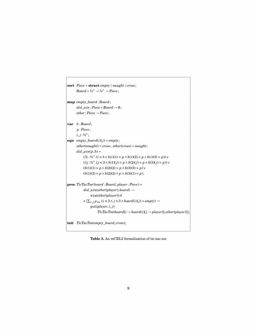
Table 3. An mCRL2 formalisation of tic-tac-toe

9

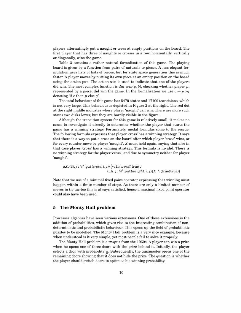
players alternatingly put a naught or cross at empty positions on the board. Thefirst player that has three of naughts or crosses in a row, horizontally, verticallyor diagonally, wins the game.

Table 3 contains a rather natural formalisation of this game. The playingboard is given by a function from pairs of naturals to pieces. A less elegant for-mulation uses lists of lists of pieces, but for state space generation this is muchfaster. A player moves by putting its own piece at an empty position on the boardusing the action put. The action win is used to indicate that one of the playersdid win. The most complex function is did_win(p,b), checking whether player p,represented by a piece, did win the game. In the formalisation we use c → p ¦ qdenoting ‘if c then p else q’.

The total behaviour of this game has 5479 states and 17109 transitions, whichis not very large. This behaviour is depicted in Figure 2 at the right. The red dotat the right middle indicates where player ‘naught’ can win. There are more suchstates two disks lower, but they are hardly visible in the figure.

Although the transition system for this game is relatively small, it makes nosense to investigate it directly to determine whether the player that starts thegame has a winning strategy. Fortunately, modal formulas come to the rescue.The following formula expresses that player ‘cross’ has a winning strategy. It saysthat there is a way to put a cross on the board after which player ‘cross’ wins, orfor every counter move by player ‘naught’, X must hold again, saying that also inthat case player ‘cross’ has a winning strategy. This formula is invalid. There isno winning strategy for the player ‘cross’, and due to symmetry neither for player‘naught’.

µX .⟨∃i, j :N+.put(cross, i, j)⟩ (⟨win(cross)⟩true∨([∃i, j :N+.put(naught, i, j)] X ∧⟨true⟩true)

)Note that we use of a minimal fixed point operator expressing that winning musthappen within a finite number of steps. As there are only a limited number ofmoves in tic-tac-toe this is always satisfied, hence a maximal fixed point operatorcould also have been used.

5 The Monty Hall problem

Processes algebras have seen various extensions. One of these extensions is theaddition of probabilities, which gives rise to the interesting combination of non-deterministic and probabilistic behaviour. This opens up the field of probabilisticpuzzles to be modelled. The Monty Hall problem is a very nice example, becausewhen understood is it very simple, yet most people fail to solve it properly.

The Monty Hall problem is a tv-quiz from the 1960s. A player can win a prizewhen he opens one of three doors with the prize behind it. Initially, the playerselects a door with probability 1

3 . Subsequently, the quizmaster opens one of theremaining doors showing that it does not hide the prize. The question is whetherthe player should switch doors to optimise his winning probability.

10

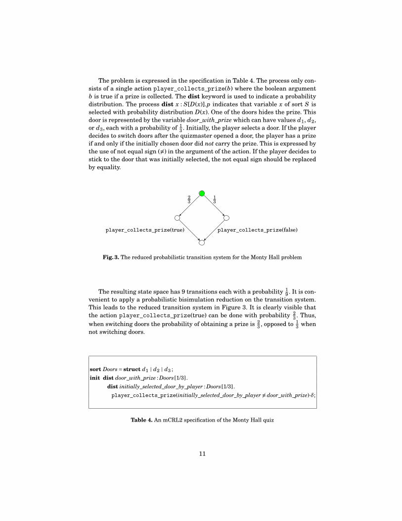
The problem is expressed in the specification in Table 4. The process only con-sists of a single action player_collects_prize(b) where the boolean argumentb is true if a prize is collected. The dist keyword is used to indicate a probabilitydistribution. The process dist x : S[D(x)].p indicates that variable x of sort S isselected with probability distribution D(x). One of the doors hides the prize. Thisdoor is represented by the variable door_with_prize which can have values d1, d2,or d3, each with a probability of 1

3 . Initially, the player selects a door. If the playerdecides to switch doors after the quizmaster opened a door, the player has a prizeif and only if the initially chosen door did not carry the prize. This is expressed bythe use of not equal sign (6≈) in the argument of the action. If the player decides tostick to the door that was initially selected, the not equal sign should be replacedby equality.

player_collects_prize(false)player_collects_prize(true)

13

23

Fig. 3. The reduced probabilistic transition system for the Monty Hall problem

The resulting state space has 9 transitions each with a probability 19 . It is con-

venient to apply a probabilistic bisimulation reduction on the transition system.This leads to the reduced transition system in Figure 3. It is clearly visible thatthe action player_collects_prize(true) can be done with probability 2

3 . Thus,when switching doors the probability of obtaining a prize is 2

3 , opposed to 13 when

not switching doors.

sort Doors= struct d1 | d2 | d3 ;init dist door_with_prize : Doors [1/3] .

dist initially_selected_door_by_player : Doors [1/3] .player_collects_prize(initially_selected_door_by_player 6≈ door_with_prize)·δ;

Table 4. An mCRL2 specification of the Monty Hall quiz

11

map N :N+ ;eqn N = 100;

proc Plane(everybody_has_his_own_seat :B, number_of_empty_seats :N )=(number_of_empty_seats≈ 0) →last_passenger_has_his_own_seat(everybody_has_his_own_seat)·δ

¦ (enter·dist b0 :B[if (everybody_has_his_own_seat, if (b0,1,0),

if (b0,1−1/number_of_empty_seats,1/number_of_empty_seats))] .b0 → select_seat·

Plane(everybody_has_his_own_seat,number_of_empty_seats−1)¦ dist b1 :B[if (b1,1/number_of_empty_seats,1−1/number_of_empty_seats)].select_seat·

Plane(if (number_of_empty_seats≈1,everybody_has_his_own_seat,b1),number_of_empty_seats−1)) ;

init dist b :B[if (b,1/N, (N −1)/N)].Plane(b, N −1);

Table 5. An mCRL2 specification of the lost boarding pass

6 The problem of the lost boarding pass

More complex probabilistic problems can become rather hard even with the fullstrength of probability theory at ones disposal. Yet modelling the problem inmCRL2 is again pretty straightforward. The tools can subsequently help to ob-tain the required answer.

A particularly intriguing puzzle is that of the lost boarding pass as it has a re-markable answer, defying the intuition of most people trying to solve the problem:There is a plane with 100 seats. The first passenger boarding the plane lost hisboarding ticket and selects a random seat. Each subsequent passenger will usehis own seat unless it is already occupied. In that case he also selects a randomseat. The question is what the probability is that the last passenger entering theplane will sit in his own seat.

The behaviour is modelled in Table 5. The number N is the number of seats,which is set to 100. The behaviour of entering the plane is characterised by two pa-rameters. The parameter number_of_empty_seats indicates how many seats arestill empty in the plane. The parameter everybody_has_his_own_seat indicatesthat all remaining seats correspond exactly with the places for all passengers

12

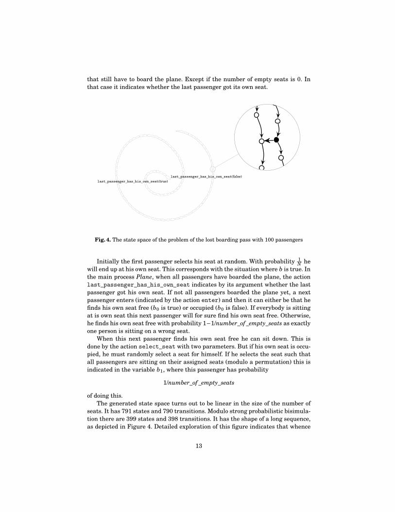
that still have to board the plane. Except if the number of empty seats is 0. Inthat case it indicates whether the last passenger got its own seat.

last_passenger_has_his_own_seat(false)last_passenger_has_his_own_seat(true)

last_passenger_has_his_own_seat(false)last_passenger_has_his_own_seat(true)

Fig. 4. The state space of the problem of the lost boarding pass with 100 passengers

Initially the first passenger selects his seat at random. With probability 1N he

will end up at his own seat. This corresponds with the situation where b is true. Inthe main process Plane, when all passengers have boarded the plane, the actionlast_passenger_has_his_own_seat indicates by its argument whether the lastpassenger got his own seat. If not all passengers boarded the plane yet, a nextpassenger enters (indicated by the action enter) and then it can either be that hefinds his own seat free (b0 is true) or occupied (b0 is false). If everybody is sittingat is own seat this next passenger will for sure find his own seat free. Otherwise,he finds his own seat free with probability 1−1/number_of_empty_seats as exactlyone person is sitting on a wrong seat.

When this next passenger finds his own seat free he can sit down. This isdone by the action select_seat with two parameters. But if his own seat is occu-pied, he must randomly select a seat for himself. If he selects the seat such thatall passengers are sitting on their assigned seats (modulo a permutation) this isindicated in the variable b1, where this passenger has probability

1/number_of_empty_seats

of doing this.The generated state space turns out to be linear in the size of the number of

seats. It has 791 states and 790 transitions. Modulo strong probabilistic bisimula-tion there are 399 states and 398 transitions. It has the shape of a long sequence,as depicted in Figure 4. Detailed exploration of this figure indicates that whence

13

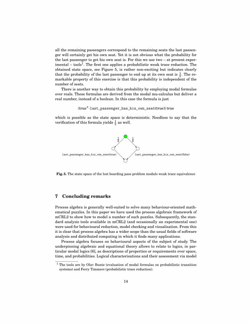
all the remaining passengers correspond to the remaining seats the last passen-ger will certainly get his own seat. Yet it is not obvious what the probability forthe last passenger to get his own seat is. For this we use two – at present exper-imental – tools1. The first one applies a probabilistic weak trace reduction. Theobtained state space, see Figure 5, is rather non-exciting but indicates clearlythat the probability of the last passenger to end up at its own seat is 1

2 . The re-markable property of this exercise is that this probability is independent of thenumber of seats.

There is another way to obtain this probability by employing modal formulasover reals. These formulas are derived from the modal mu-calculus but deliver areal number, instead of a boolean. In this case the formula is just

⟨true?·last_passenger_has_his_own_seat(true)⟩true

which is possible as the state space is deterministic. Needless to say that theverification of this formula yields 1

2 as well.

last_passenger_has_his_own_seat(false)last_passenger_has_his_own_seat(true)

12

12

Fig. 5. The state space of the lost boarding pass problem modulo weak trace equivalence

7 Concluding remarks

Process algebra is generally well-suited to solve many behaviour-oriented math-ematical puzzles. In this paper we have used the process algebraic framework ofmCRL2 to show how to model a number of such puzzles. Subsequently, the stan-dard analysis tools available in mCRL2 (and occasionally an experimental one)were used for behavioural reduction, model checking and visualisation. From thisit is clear that process algebra has a wider scope than the usual fields of softwareanalysis and distributed computing in which it finds many applications.

Process algebra focuses on behavioural aspects of the subject of study. Theunderpinning algebraic and equational theory allows to relate to logics, in par-ticular modal logics [6], as descriptions of properties or requirements over space,time, and probabilities. Logical characterisations and their assessment via model

1 The tools are by Olav Bunte (evaluation of modal formulas on probabilistic transitionsystems) and Ferry Timmers (probabilistic trace reduction).

14

checking are a valuable replacement in situations where visual techniques, high-lighted for the puzzles discussed here, become impractical.

Also other authors indicated that a notion of behaviour or state space is re-quired for proper conditional reasoning, especially in the probabilistic setting.In [19] the distinction is made between ‘naive’ and ‘sophisticated’ space. For theMonty Hall puzzle this amounts to the three doors for the naive space, and to se-quences of events for the sophisticated space. In the process algebraic modelling ofthe problem, it is exactly the latter that is determined by the specified behaviour,thus making the underlying protocol explicit.

Although we defend the use of process algebra as a qualitatively better ap-proach to solving behavioural problems, this is a subjective opinion, influencedby our experience with process algebras. To substantiate this in a more objec-tive manner one should measure how much time people need to solve particularproblems with particular techniques, for instance by psychological tests.

If process algebraic techniques become commonplace, it might be that the na-ture of ‘tricky’ puzzles will shift where the proper behaviour is not directly obvi-ous. Nice examples are for instance Freudenthal problems, containing knowledge,like the Muddy Children puzzle [11]. Translating knowledge into behaviour oftenrequires a twist. In such cases dynamic epistemic logic might be more suitable [9].

Acknowledgement. The authors are grateful to the reviewers for their construc-tive and inspiring comments.

References

1. Alcuinus Flaccus. Propositiones ad Acuendos Juvenes. Manuscript. 780.2. H. Bekic. Towards a mathematical theory of processes. Technical Report TR25.125,

IBM Laboratory, Vienna, 1971. Also appeared in Programming Languages and TheirDefinition, C.B. Jones (ed.), Lecture Notes in Computer Science 177, Springer, 1984.

3. J.A. Bergstra and J.W. Klop. Fixed point semantics in process algebras. Report IW 206,Mathematisch Centrum, Amsterdam, 1982.

4. J.A. Bergstra and J.W. Klop. Process algebra for synchronous communication. Infor-mation and Computation 60(1/3):109–137, 1984.

5. F. Biemans and P. Blonk. On the formal specification and verification of CIM architec-tures using LOTOS. Computers in Industry 7(6), 491–504, 1986.

6. P. Blackburn, J. van Benthem, and F. Wolter (eds.). Handbook of Modal Logic. Studiesin Logic and Practical Reasoning volume 3. Elsevier, 2007.

7. E. Brinksma and G. Karjoth. A specification of the OSI transport service in LOTOS. InProtocol Specification, Testing and Verification IV. Y. Yemini, R.E. Strom and S. Yemini(eds), pp. 227–251. North-Holland, 1984.

8. E.M. Clarke and E.A. Emerson. Design and synthesis of synchronization skeletonsusing branching time temporal logic. In Logic of Programs, D. Kozen (ed.), pp. 52–71.Lecture Notes in Computer Science 131, Springer, 1981.

9. H. van Ditmarsch, W. van der Hoek, and B. Kooij. Dynamic Epistemic Logic. Studiesin Epistemology, Logic, Methodology, and Philosophy of Science volume 337. Springer,2008.

10. E.W. Dijkstra. Pruning the search tree. EWD1255. Available at www.cs.utexas.edu/users/EWD/transcriptions/EWD12xx/EWD1255.html. Accessed June 2017.

15

11. P. van Emde Boas, J. Groenendijk, and M. Stokhof. The Conway paradox: Its solutionin an epistemic framework. In Truth, Interpretation, and Information: Selected Pa-pers from the Third Amsterdam Colloquium. J. Groenendijk, T.M.V. Janssen, and M.Stokhof (eds.), pp. 159–182. Foris Publications, 1984.

12. H. Garavel, F. Lang, R. Mateescu, and W. Serwe. CADP 2011: A toolbox for the con-struction and analysis of distributed processes. International Journal on SoftwareTools for Technology Transfer 15(2):89–107, 2013

13. M. Gardner. My best mathematical and logic puzzles. Dover, 1994.14. T. Gibson-Robinson, P. Armstrong, A. Boulgakov, and A.W. Roscoe. FDR3 — A Modern

Refinement Checker for CSP. In Tools and Algorithms for the Construction and Anal-ysis of Systems, E. Abraham and K. Havelund (eds.), pp. 187–201. Lecture Notes inComputer Science 8413, 2014.

15. S. Cranen, J.F. Groote, and M.A. Reniers. A linear translation from CTL* to the first-order modal mu-calculus. Theoretical Computer Science 412(28):3129–3139, 2011.

16. J.F. Groote and F. van Ham. Interactive visualization of large state spaces. Interna-tional Journal on Software Tools for Technology Transfer 8(1):77–91, 2006.

17. J.F. Groote and M.R. Mousavi. Modeling and Analysis of Communication Systems. TheMIT Press 2014. (See for the toolset www.mcrl2.org).

18. J.F. Groote and A. Ponse. The syntax and semantics of µCRL. Report CS-R9076, CWI,Amsterdam, 1990.

19. P. Grünwald and J.Y. Halpern. Updating Probabilities. In Uncertainty in Artificial In-telligence, A. Darwiche and N. Friedman (eds.), pp. 187–196. Morgan Kaufman, 2002.

20. M.C.B. Hennessy and R. Milner. On observing nondeterminism and concurrency.In Automata, Languages and Programming (ICALP’80), J.W. de Bakker and J. vanLeeuwen (eds.), pp. 299–309. Lecture Notes in Computer Science 85, Springer, 1980.

21. C.A.R. Hoare. Communicating sequential processes. Communications of the ACM21(8):666–677, 1978.

22. C.A.R. Hoare. Communicating sequential processes. Prentice Hall International, 1985.23. D. Kozen. Results on the propositional µ-calculus. Theoretical Computer Science,

27:333–354, 1983.24. ISO 8807:1989. Information processing systems – Open Systems Interconnection –

LOTOS – A formal description technique based on the temporal ordering of observa-tional behaviour. ISO/IECJTC1/SC7 1989.

25. R. Milner. An approach to the semantics of parallel programs. In Proceedings Con-vegno di Informatica Teorica, Pisa, pp. 283–302, 1973.

26. S. Mauw and G.J. Veltink. A process specification formalism. Fundamenta Informati-cae, XIII:85–139, 1990.

27. R. Milner. Processes: A mathematical model of computing agents. In Proceedings LogicColloquium 1972, H.E. Rose and J.C. Shepherdson (eds.), pp. 158–173. North-Holland,1973.

28. R. Milner. A calculus of communicating systems. Lecture Notes in Computer Science92, Springer, 1979.

29. A. Pnueli. The temporal logic of programs. In Foundations of Computer Science, pp. 46-57. IEEE, Piscataway, 1977.

30. A.N. Prior. Time and modality. Oxford University Press, 1957.31. A.W. Roscoe. Understanding concurrent systems. Springer, 2010.32. M. van Sinderen, I. Ajubi, and F. Caneschi. The application of LOTOS for the formal

description of the ISO session layer. In Formal Description Techniques, K.J. Turner(ed.), pp. 263–277. North-Holland, 1989.

33. P. Winkler. Mathematical Puzzles. A connaisseur’s collection. A.K. Peters, 2004.

16