10th World Congress on Structural and Multidisciplinary Optimization

May 19 -24, 2013, Orlando, Florida, USA

1

Probability Collectives for Solving Truss Structure Problems

Anand J. Kulkarni1,2, Ishaan R. Kale

1 and K. Tai

2

1 Optimization and Agent Technology (OAT) Research Lab

Maharashtra Institute of Technology, Pune 411038, India

E-mail: {ajkulkarni, irkale}@oatresearch.org

2 School of Mechanical and Aerospace Engineering

Nanyang Technological University, 50 Nanyang Avenue, Singapore 639798

E-mail: {kulk0003, mktai}@ntu.edu.sg

1. Abstract

The approach of Probability Collectives (PC) in the Collective Intelligence (COIN) framework is one of the

emerging Artificial Intelligence approaches dealing with the complex problems in a distributed way. It decomposes

the entire system into subsystems and treats them as a group of learning, rational and self interested agents or a

Multi-Agent System (MAS). These agents iteratively select their strategies to optimize their individual local goal

which also makes the system to achieve the global optimum. The approach of PC has been tested and validated by

solving a variety of practical problems in continuous domain. This paper demonstrates the ability of PC solving 2-D

space truss structure and 3-D truss structure design problems with discrete as well as continuous variables. The

approach is shown to be producing competent and sufficiently robust results. The associated strengths, weaknesses

are also discussed. The solution to these problems indicates that the approach of PC can be further efficiently

applied to solve a variety of practical/real world problems.

2. Keywords: Probability Collectives, Collective Intelligence, Multi-Agent System, Discrete Variable Problems

3. Introduction

In the framework of Collective Intelligence (COIN), the Artificial Intelligence (AI) tool referred to as Probability

Collectives (PC) is becoming popular for modeling and controlling distributed Multi-Agent System (MAS) [1-15].

It was inspired from a sociophysics viewpoint, with deep connections to Game Theory, Statistical Physics, and

Optimization [1, 2]. According to [1, 2, 9-11], the key characteristics of the PC methodology such as its ability to

accommodate discrete and continuous variables as well as irregular and noisy functions, tolerance to

subsystem/agent failure, ability to provide sensitivity information and ability to handle uncertainty in terms of

probability, use of homotopy function to make the solution jump out of possible local minima, ability to avoid the

tragedy of commons, high scalability, ability to achieve unique Nash Equilibrium, etc. makes it a very competitive

choice over other contemporary algorithms. The approach of PC has been applied in variegated areas such as

airplane fleet assignment problem [12] and various cases of the Multiple Traveling Salesmen Problems (MTSPs)

[4, 7], continuous constrained problems such as benchmark test problems [7, 9, 13-15], two variations of the Circle

Packing Problem (CPP) [5], Sensor Network Coverage Problem [10] as well as fault-tolerant system in association

with the CPP [11]. Furthermore, the segmented beam problem [8], multimodal, nonlinear and non-separable test

problems comparing the performance with Genetic Algorithm (GA) [24] as well as joint optimization of the

routing and resource allocation in wireless networks [16-23] have been solved as continuous unconstrained

problems. In addition, performance of the centralized and decentralized architectures of PC was evaluated solving

continuous unconstrained 8-Queens problem [24] which underscored superiority of the decentralized approach of

PC methodology.

The approach of PC has been applied solving discrete constrained problem such as university course scheduling

[16] in which the PC approach was failed to generate any feasible solution. Importantly, in order to explore the

ability of PC solving real world mechanical engineering problems, its potential needs to be tested solving

continuous and discrete variable problems. This paper intends to validate and explore the ability of PC solving

three truss structure design problems with continuous and discrete variables. The truss structure problems such as

17-Bar, two cases of 25-Bar and 72-Bar each were successfully solved and results were validated by comparing

with the other contemporary algorithms. The robust and competent results validated the strong potential of PC

methodology solving further real world practical problems with discrete variables.

The paper is organized as follows. Section 4 discusses the framework and detailed formulation of the constrained

PC approach. The validation of the PC approach solving continuous and discrete truss structure problem is

presented in Section 5 along with the solution comparison with other contemporary algorithms. The evident

features, advantages and limitations of the constrained PC approach are discussed in Section 6 along with the

2

concluding remarks and future work.

4. Conceptual Framework of Constrained PC

PC treats the variables in an optimization problem as individual self interested learning agents/players of a game

being played iteratively. While working in some definite direction, these agents select actions over a particular

interval and receive some local rewards on the basis of the system objective achieved because of those actions. In

other words, these agents optimize their local rewards or payoffs, which also optimize the system level

performance. The process iterates and reaches equilibrium (referred to as Nash equilibrium) when no further

increase in the reward is possible for the individual agent through changing its actions further. Moreover, the

method of PC theory is an efficient way of sampling the joint probability space, converting the problem into the

convex space of probability distribution. PC allocates probability values to each agent’s moves, and hence directly

incorporates uncertainty. This is based on prior knowledge of the recent action or behavior selected by all other

agents. In short, the agents in the PC framework need to have knowledge of the environment along with every

other agent’s recent action or behavior.

In every iteration, each agent randomly samples the actions/moves/strategies from within its own strategy set (i.e.

its own sampling interval) as well as from within other agents’ strategy sets and computes the corresponding

system objectives. The other agents’ strategy sets are modeled by each agent based on their recent actions or

behavior only, i.e. based on partial knowledge. By minimizing the collection of system objectives, every agent

identifies the possible strategy which contributes the most towards the minimization of the collection of system

objectives. Such a collection of functions is computationally expensive to minimize and also may lead to local

minima. In order to avoid this difficulty, the collection of system objectives is deformed into another topological

space forming the homotopy function parameterized by computational temperature T . Due to its analogy to

Helmholtz free energy [9], the approach of Deterministic Annealing (DA) converting the discrete variable space

into continuous variable space of probability distribution is applied in minimizing the homotopy function. At every

successive temperature drop, the minimization of the homotopy function is carried out using a second order

optimization scheme such as the Nearest Newton Descent Scheme [3] or Broyden-Fletcher-Goldfarb-Shanno

(BFGS) Scheme [5], etc.

At the end of every iteration, each agent i converges to a probability distribution clearly distinguishing the

contribution of its every corresponding strategy. For every agent, the strategy with the maximum probability value

is referred to as the favourable strategy and is used to compute the system objective and corresponding constraint

functions. This system objective and corresponding strategies are accepted based on the feasibility-based rule [5,

11]. This rule allows the objective function and the constraint information to be considered separately. The rule can

be described as follows:

1. Any feasible solution is preferred over any infeasible solution

2. Between two feasible solutions, the one with better objective is preferred

3. Between two infeasible solutions, the one with more number of improved constraint violations is preferred.

In addition, once the solution becomes feasible, the sampling space of every agent is shrunk to the local

neighborhood of its favorable strategy. In this way, the algorithm continues until convergence by selecting the

samples from the neighbourhood of the recent favourable strategies. The following section discusses the

constrained PC procedure in detail.

4.1. Constrained PC Algorithm

Consider the general constrained problem (in minimization case) as follows:

Minimize G (1)

Subject to 0, 1, 2, ...,jg j s≤ =

0, 1, 2, ...,jh j w= =

and associated constraint vector represented as [ ]1 2 1 2C , ,..., , , , ...,s wg g g h h h=

In PC algorithm, the variable of the problem is considered as computational agent/player of a social game being

played iteratively [2, 3]. Each agent i given a strategy [ ] , 1, 2, 3, ...,r

i iX r m= from predefined sampling interval

,l u

i i i Ψ = Ψ Ψ is referred as interval where l

iΨ is lower limit and u

iΨ is upper limit, from which each agent

selects its strategy and form a strategy set Xi represented as,

{ }[ ][1] [2] [3]X , , , ..., , 1, 2, 3, ...,im

i i i i iX X X X i N= = (2)

Every agent selects equal number of strategies i.e. 1 2 1... ...i N Nm m m m m−= = = = = = . The procedure of modified

PC theory is explained below in detail with the algorithm flowchart in Figure 1.

3

The procedure begins with the initialization of the sampling interval iΨ for each agent i , computational

temperature 0T >> or T → ∞ , temperature step size ( )0 1T Tα α< ≤ , algorithm iteration counter 1n = and

number of iterationtestn . The value of and T testnα are selected depending on preliminary trials of algorithm.

Furthermore, the constraint violation tolerance µ is initialized to number of constraints C , i.e. Cµ = , where

C refers to the cardinality of the constraint vector C .

Step 1. Agent i selects its first strategy [1]

iX and samples randomly from other agents strategies. These are the

random guess by agent i . Thus every agent i form the combined strategy set [1]Yi

for agent i represented as,

{ }[ ] [?] [?] [ ] [?] [?]

1 2 1Y , , ..., , ..., , r r

i i N NX X X X X−= (3)

The superscript [?] indicates the random guess of strategies for other agents.

Step 2. For each of its combined strategy set [ ]Y

r

i such agent i computes im objective function values as follows,

( ) ( ) ( ) ( )[ ][1] [2] [ ]Y , Y , ..., Y , ..., Y imr

i i i iG G G G

(4)

The major goal of every agent i is to identify the strategy which contributes most towards the minimization of the

sum of these objective systems i.e. the collection of system objective ( )[ ]

1

Yim

r

i

r

G=∑ .

Step 3. Minimization of function ( )[ ]

1

Yim

r

i

r

G=∑ is more cumbersome to achieve, as it may have many possible local

minima as it may need excessive computational effort [3]. One way to deal with this difficulty is to deform the

function into another topological space by constructing the easier function ( )Xi

f , such method is referred as

homotopy method [27-30]. Such function is easy to compute the global optimum value [27-29]. The deformed

function can also be referred as homotopy function J , parameterized by computational temperature T as defined

earlier, represented as,

( ) ( ) ( ) [ )[ ]

1

X , Y X , 0,im

r

i i i i

r

J T G T f T=

= + ∈ ∞∑ (5)

Further, the suitable function for ( )if X is chosen. The general choice is iS referred as entropy function [26-28]

( ) ( )[ ] [ ]

2

1

logim

r r

i i i

r

S q X q X=

= −∑ (6)

a) At the beginning of the game, least information is available so it seems too difficult to select the best strategy.

Therefore agent i selects uniform probability for its strategies. Each agent’s every strategy has probability 1 im

or being most favorable. Thus probability of r strategies will be,

( )[ ]X 1 , 1, 2, ...,r

i i iq m r m= = (7)

and further computes im corresponding system objective values ( )( )[ ]Y r

iE G as follows,

( )( ) ( ) ( ) ( )( )

[ ] [ ] [ ] [?]

( )Y r r r

i i i i

i

E G G Y q X q X= ∏ (8)

where ( )i represents, every agent other than i . Thus every agent compute collection of expected system

objective values denoted as ( )( )[ ]

1

Yim

r

i

r

E G=∑ .

b) It seems that PC approach can convert any discrete variable into continuous variable values in the form of

probabilities corresponding to discrete variable. The problem now becomes continuous but still not easier to

compute.

Thus the homotopy function to be minimized by each agent i is modified as follows:

( )( ) ( )( )[ ]

1

X , Y im

r

i i i i

r

J q T E G T S=

= −∑ (9)

To minimize the homotopy function, Nearest Newton Descent Scheme was implemented [3].

4

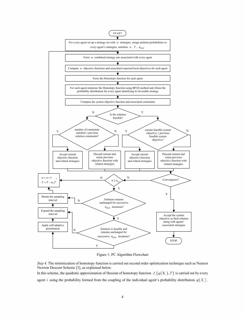
Figure 1: PC Algorithm Flowchart

Step 4. The minimization of homotopy function is carried out second order optimization technique such as Nearest

Newton Descent Scheme [3], as explained below.

In this scheme, the quadratic approximation of Hessian of homotopy function ( )( )X ,i iJ q T is carried out by every

agent i using the probability formed from the coupling of the individual agent’s probability distribution ( )iq X .

current feasible system objective ≤ previous

feasible system

objective?

Y

testn n≥

START

For every agent set up a strategy set with m strategies, assign uniform probabilities to

every agent’s strategies, initialize n , T , testn

Form m combined strategy sets associated with every agent

Form the Homotopy function for each agent

For each agent minimize the Homotopy function using BFGS method and obtain the

probability distribution for every agent identifying its favorable strategy

Accept current

objective function

and related strategies

Y

Discard current and retain previous

objective function with

related strategies

STOP

Accept the system objective as final solution

along with agents’

associated strategies

N

Compute the system objective function and associated constraints

Is the solution

feasible?

Compute m objective functions and associated expected local objectives for each agent

Y N number of constraints

satisfied ≥ previous

solution constraints?

Accept current

objective function

and related strategies

Discard current and retain previous

objective function with

related strategies

Y N

N

Solution remains unchanged for successive

testn iterations?

Expand the sampling

interval

Shrink the sampling

interval

Y

N

Solution is feasible and remains unchanged for

successive testn iterations?

Apply self-adaptive

perturbation

Convergence?

N

1n n= + ,

TT T Tα= −

N

Y

Y

5

The simplified resulting probability update rule for each strategy r of agent i , referred to as ‘k-update rule’ [1-4]

which minimize the homotopy function in Eq. (9), is represented as;

( ) ( ) ( )1[ ] [ ] [ ]

.

k k kr r r

i i step i r updateq X q X q X kα+

← − (10)

( )( )( )

( ) ( )( )( ) ( )( )

[ ]

[ ]

. 2

[ ] [ ] [ ]

1

where log

and Y Yi

kr

ki k r

r update i i

kmkk

r r r

i i i

r

Contribution of Xk S q X

T

Contribution of X E G E G=

= + +

= −

∑

where k is the corresponding update is number (iteration) and ( )kiS is the corresponding entropy. The updating

procedure is as follows:

a) Set number of iteration 1k = , maximum number of update finalk , and step size ( )0 1step stepα α< ≤ . The value

of finalk and

stepα are held constant throughout the operation.

b) Update every agent’s probability distribution ( )kiq X using update rule.

c) If finalk k≥ , stop and go to step 5, else update 1k k= + and return to (b).

Step 5. For each agent i the above minimization process converges the probability distribution of every strategy.

Which can be seen as a individual agent probability distribution clearly distinguish every strategies contribution

towards the minimization for the expected collection of system objectives ( )( )[ ]

1

Yim

r

i

r

E G=∑ .

In other words, for every agent i if the strategy contributes more towards the minimization of the objective

compared to other strategies, its corresponding probability certainly increases by some amount more than those for

the other strategies probability values, so that strategy r distinguished from the other strategies. Such a strategy

referred as favorable strategy [ ]fav

iX . Thus it forms corresponding favorable combined strategy set [ ]Y

fav

i and

favorable system objective ( )[ ]Y fav

iG .

Step 6. This fourable solution is selected on following selection criterion:

a) If the constraint violated violatedC µ≤ , accept the current solution and set

violatedC µ= ,and continue to Step 7.

b) If violatedC µ> , discard the current solution and retain the previous iteration solution, continue to Step 7.

c) If current solution is feasible i.e. 0violatedC µ= = and is not worse than previous feasible solution then accept the

current solution and continue to Step 7, else discard the current solution and retain the previous solution and

continue to Step 7.

Step 7. On the completion of per-specified testn iterations, the following condition is checked for every further

iteration, i.e. ( ) ( )[ ],[ ],Y Y testfav n nfav nG G−≤ , then every agent i shrinks its sampling interval to the local

neighborhood of its current favorable strategy [ ]fav

iX using the interval factor λ . In otherwords, for agent i , λ

strategies on either side of the current favorable strategy [ ]fav

iX inclusive, will be available for the following

iteration of the algorithm.

Step8: Each agent i then samples im strategies from within the updated sampling interval and form the

corresponding updated strategy set Xi represented as follows:

{ }[ ][1] [2] [3]X , , ..., , 1, 2, 3, ...,im

i i i i iX X X X i N= = (11)

Reduce the temperature TT T Tα= − , iteration 1n n= + and go to Step 1.

5. Solved Problems

To test the constrained PC approach, three structural optimization problems were considered such as 17 bar, two

cases 25 bar and 72 bar, respectively. The 17 bar problem was considered as a continuous whereas; 25 bar and 72

bar problems were considered as a discrete optimization problems. These problems were previously solved using

variegated nature inspired approaches such as Genetic Algorithm (GA) [31, 32], , Harmony Search (HS) [33, 34],

Particle Swarm Optimization (PSO), PSO with Passive Congregation (PSOPC), Hybrid PSO [35, 36], Discrete

Heuristic Particle Swarm Ant Colony Optimization (DHPSACO) [37], etc.

Various approaches were proposed with their merits and demerits to handle the discrete constrained optimization

problems. The Steady State Genetic Algorithms (SSGAs) approach was proposed to solve the discrete truss

6

structure problems using binary digit string to design variables so that to achieve the minimum function

evaluations and to make the approach more efficient. The penalty-function method and augmented Lagrangian

approach [32] were used with Preconditioned Conjugate Gradient search because of its low memory requirement

and ultimately it increase the computational speed and reduce the time for the same. The Harmony Search

algorithm [33, 34] shows the comparison between aesthetic musical composition and optimization processes to

determine the global system objective with using both continuous and discrete sizing variables. The discrete

optimization problems were also solved using Hybrid Particle Swarm Optimization (HPSO) [35, 36], fly-back

mechanism [35] were used for Pin Connected Structures as a constraint handling technique to improve the

convergence rate and accuracy of problem solving and in [36] the combination of PSO and HS was proposed to

solve the discrete optimization problems to get the faster convergence of system objective than PSO and PSOPC.

The Hybridization of PSOPC, ACO and HS was proposed to get discrete version of HPSACO (i.e. DHPSACO)

[37] which reduces the search space of the design variables to get faster optimum solution incorporating

terminating criteria to eliminate the unnecessary iterations.

In this current work, the constrained PC algorithm was coded in MATLAB 7.7.0 (R2008b) and the simulations

were run on Windows platform using an Intel Core i5, 2.8GHz processor speed and 4GB RAM. The mathematical

formulation, results and comparison of solved problems with other contemporary algorithm are discussed below.

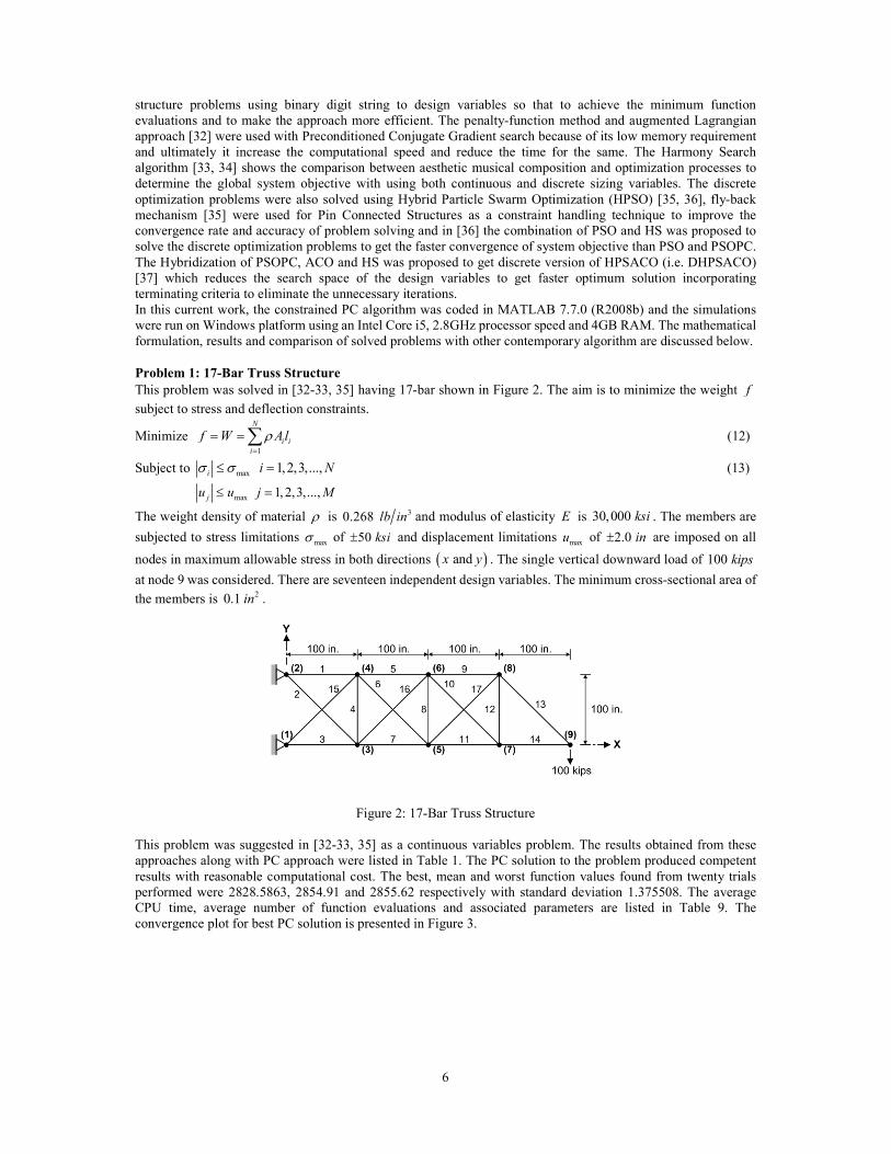
Problem 1: 17-Bar Truss Structure

This problem was solved in [32-33, 35] having 17-bar shown in Figure 2. The aim is to minimize the weight f

subject to stress and deflection constraints.

Minimize 1

N

i i

i

f W Alρ=

= =∑ (12)

Subject to max 1,2,3,...,

ii Nσ σ≤ = (13)

max 1, 2,3,...,ju u j M≤ =

The weight density of material ρ is 30.268 lb in and modulus of elasticity E is 30,000 ksi . The members are

subjected to stress limitations maxσ of 50 ksi± and displacement limitations

maxu of 2.0 in± are imposed on all

nodes in maximum allowable stress in both directions ( ) and x y . The single vertical downward load of 100 kips

at node 9 was considered. There are seventeen independent design variables. The minimum cross-sectional area of

the members is 20.1 in .

Figure 2: 17-Bar Truss Structure

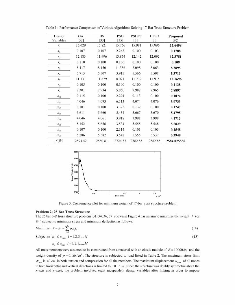
This problem was suggested in [32-33, 35] as a continuous variables problem. The results obtained from these

approaches along with PC approach were listed in Table 1. The PC solution to the problem produced competent

results with reasonable computational cost. The best, mean and worst function values found from twenty trials

performed were 2828.5863, 2854.91 and 2855.62 respectively with standard deviation 1.375508. The average

CPU time, average number of function evaluations and associated parameters are listed in Table 9. The

convergence plot for best PC solution is presented in Figure 3.

7

Table 1: Performance Comparison of Various Algorithms Solving 17-Bar Truss Structure Problem

Design

Variables

GA

[32]

HS

[33]

PSO

[35]

PSOPC

[35]

HPSO

[35] Proposed

PC

1x 16.029 15.821 15.766 15.981 15.896 15.6498

2x 0.107 0.107 2.263 0.100 0.103 0.1788

3x 12.183 11.996 13.854 12.142 12.092 12.3751

4x 0.110 0.100 0.106 0.100 0.100 0.109

5x 8.417 8.150 11.356 8.098 8.063 8.3895

6x 5.715 5.507 3.915 5.566 5.591 5.3713

7x 11.331 11.829 8.071 11.732 11.915 12.1696

8x 0.105 0.100 0.100 0.100 0.100 0.1138

9x 7.301 7.934 5.850 7.982 7.965 7.8897

10x 0.115 0.100 2.294 0.113 0.100 0.1074

11x 4.046 4.093 6.313 4.074 4.076 3.9733

12x 0.101 0.100 3.375 0.132 0.100 0.1247

13x 5.611 5.660 5.434 5.667 5.670 5.4795

14x 4.046 4.061 3.918 3.991 3.998 4.1713

15x 5.152 5.656 3.534 5.555 5.548 5.5829

16x 0.107 0.100 2.314 0.101 0.103 0.1548

17x 5.286 5.582 3.542 5.555 5.537 5.3948

( )f lb 2594.42 2580.81 2724.37 2582.85 2582.85 2584.025556

Figure 3: Convergence plot for minimum weight of 17-bar truss structure problem

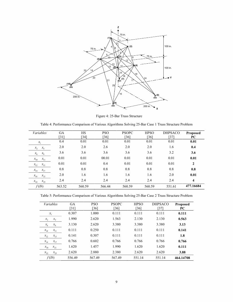
Problem 2: 25-Bar Truss Structure

The 25 bar 3-D truss structure problem [31, 34, 36, 37] shown in Figure 4 has an aim to minimize the weight f (or

W ) subject to minimum stress and minimum deflection as follows:

Minimize 1

N

i i

i

f W A lρ=

= = ∑ (14)

Subject to max 1,2,3,...,i i Nσ σ≤ = (15)

max 1,2,3,...,

ju u j M≤ =

All truss members were assumed to be constructed from a material with an elastic module of 10000E ksi= and the

weight density of 30.1 /lb inρ = . The structure is subjected to load listed in Table 2. The maximum stress limit

maxσ is 40 ksi in both tension and compression for all the members. The maximum displacement maxu of all nodes

in both horizontal and vertical directions is limited to 0.35 in± . Since the structure was doubly symmetric about the

x-axis and y-axes, the problem involved eight independent design variables after linking in order to impose

0 0.5 1 1.5 2 2.5

x 104

2500

3000

3500

4000

4500

5000

5500

Iterations

Truss Weight 'f' (lb)

8

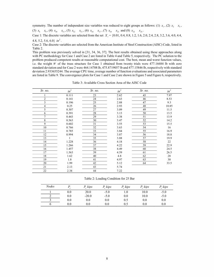
symmetry. The number of independent size variables was reduced to eight groups as follows: (1) 1x , (2) 2 5x x� ,

(3) 6 9x x� , (4)

10 11x x� , (5) 12 13x x� , (6)

14 17x x� , (7) 18 21x x� and (8)

22 25x x� .

Case 1: The discrete variables are selected from the set iX = {0.01, 0.4, 0.8, 1.2, 1.6, 2.0, 2.4, 2.8, 3.2, 3.6, 4.0, 4.4,

4.8, 5.2, 5.6, 6.0} 2in .

Case 2: The discrete variables are selected from the American Institute of Steel Construction (AISC) Code, listed in

Table 2.

This problem was previously solved in [31, 34, 36, 37]. The best results obtained using these approaches along

with PC methodology for Case 1 and Case 2 are listed in Table 4 and Table 5, respectively. The PC solution to the

problem produced competent results at reasonable computational cost. The best, mean and worst function values,

i.e. the weight W of the truss structure for Case 1 obtained from twenty trials were 477.16684 lb with zero

standard deviation and for Case 2 were 464.14708 lb, 475.8719057 lb and 477.15846 lb, respectively with standard

deviation 2.933655244. The average CPU time, average number of function evaluations and associated parameters

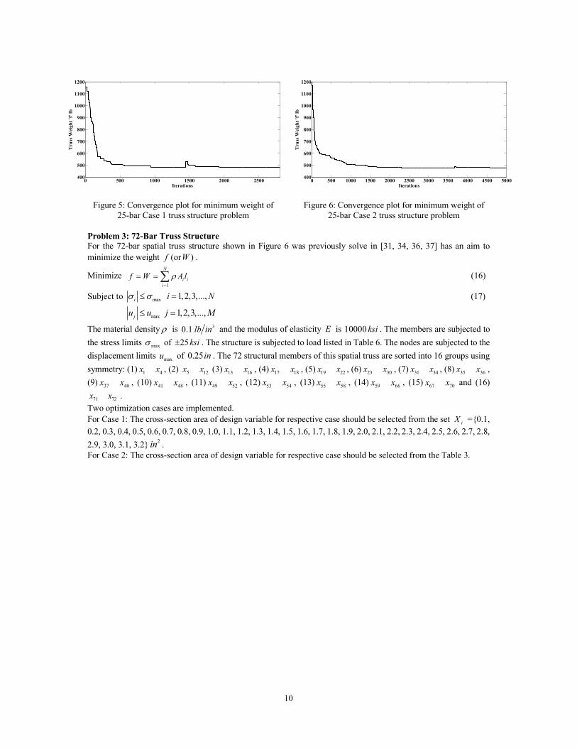
are listed in Table 9. The convergence plots for Case 1 and Case 2 are shown in Figure 5 and Figure 6, respectively.

Table 3: Available Cross Section Area of the AISC Code

Sr. no. 2in Sr. no. 2in Sr. no. 2in

1 0.111 23 2.62 45 7.97

2 0.141 24 2.63 46 8.53

3 0.196 25 2.88 47 9.3

4 0.25 26 2.93 48 10.85

5 0.307 27 3.09 49 11.5

6 0.391 28 3.13 50 13.5

7 0.443 29 3.38 51 13.9

8 0.563 30 3.47 52 14.2

9 0.602 31 3.55 53 15.5

10 0.766 32 3.63 54 16

11 0.785 33 3.84 55 16.9

12 0.994 34 3.87 56 18.8

13 1 35 3.88 57 19.9

14 1.228 36 4.18 58 22

15 1.266 37 4.22 59 22.9

16 1.457 38 4.49 60 24.5

17 1.563 39 4.59 61 26.5

18 1.62 40 4.8 62 28

19 1.8 41 4.97 63 30

20 1.99 42 5.12 64 33.5

21 2.13 43 5.74

22 2.38 44 7.22

Table 2: Loading Condition for 25 Bar

Nodes xP yP kips

zP kips xP kips yP kips zP kips

1 0.0 20.0 -5.0 1.0 10.0 -5.0

2 0.0 -20.0 -5.0 0.0 10.0 -5.0

3 0.0 0.0 0.0 0.5 0.0 0.0

6 0.0 0.0 0.0 0.5 0.0 0.0

9

Figure 4: 25-Bar Truss Structure

Table 4: Performance Comparison of Various Algorithms Solving 25-Bar Case 1 Truss Structure Problem

Variables GA

[31]

HS

[34]

PSO

[36]

PSOPC

[36]

HPSO

[36]

DHPSACO

[37] Proposed

PC

1x 0.4 0.01 0.01 0.01 0.01 0.01 0.01

2 5x x� 2.0 2.0 2.6 2.0 2.0 1.6 0.4

6 9x x� 3.6 3.6 3.6 3.6 3.6 3.2 3.6

10 11x x� 0.01 0.01 00.01 0.01 0.01 0.01 0.01

12 13x x� 0.01 0.01 0.4 0.01 0.01 0.01 2

14 17x x� 0.8 0.8 0.8 0.8 0.8 0.8 0.8

18 21x x� 2.0 1.6 1.6 1.6 1.6 2.0 0.01

22 25x x� 2.4 2.4 2.4 2.4 2.4 2.4 4

( )f lb 563.52 560.59 566.44 560.59 560.59 551.61 477.16684

Table 5: Performance Comparison of Various Algorithms Solving 25-Bar Case 2 Truss Structure Problem

Variables GA

[31]

PSO

[36]

PSOPC

[36]

HPSO

[36]

DHPSACO

[37] Proposed

PC

1x 0.307 1.000 0.111 0.111 0.111 0.111

2 5 x x� 1.990 2.620 1.563 2.130 2.130 0.563

6 9 x x� 3.130 2.620 3.380 3.380 3.380 3.13

10 11 x x� 0.111 0.250 0.111 0.111 0.111 0.141

12 13 x x� 0.141 0.307 0.111 0.111 0.111 1.8

14 17 x x� 0.766 0.602 0.766 0.766 0.766 0.766

18 21x x� 1.620 1.457 1.990 1.620 1.620 0.111

22 25 x x� 2.620 2.880 2.380 2.620 2.620 3.88

( )f lb 556.49 567.49 567.49 551.14 551.14 464.14708

10

Figure 5: Convergence plot for minimum weight of

25-bar Case 1 truss structure problem

Figure 6: Convergence plot for minimum weight of

25-bar Case 2 truss structure problem

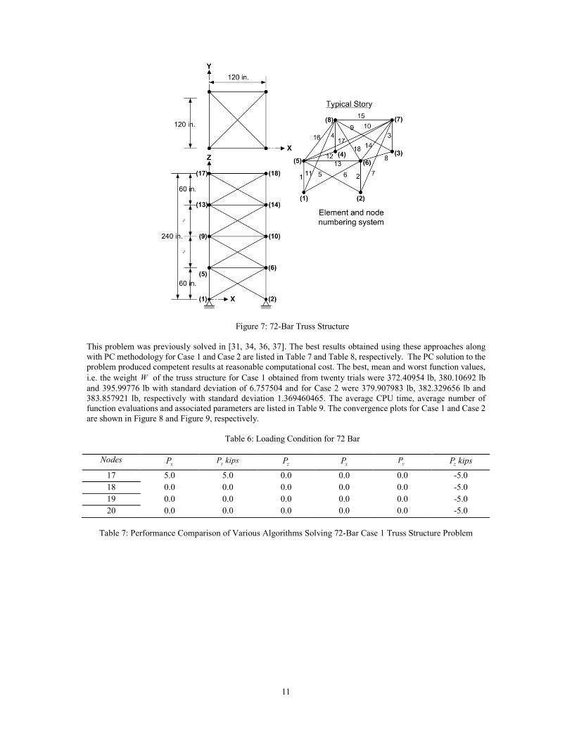
Problem 3: 72-Bar Truss Structure

For the 72-bar spatial truss structure shown in Figure 6 was previously solve in [31, 34, 36, 37] has an aim to

minimize the weight (or )f W .

Minimize 1

N

i i

i

f W A lρ=

= = ∑ (16)

Subject to max 1,2,3,...,i i Nσ σ≤ = (17)

max 1,2,3,...,

ju u j M≤ =

The material density ρ is 30.1 lb in and the modulus of elasticity E is 10000 ksi . The members are subjected to

the stress limits maxσ of 25ksi± . The structure is subjected to load listed in Table 6. The nodes are subjected to the

displacement limits maxu of 0.25in . The 72 structural members of this spatial truss are sorted into 16 groups using

symmetry: (1) 1 4x x� , (2) 5 12x x� (3) 13 16x x� , (4) 17 18x x� , (5) 19 22x x� , (6) 23 30x x� , (7) 31 34x x� , (8) 35 36x x� ,

(9)37 40x x� , (10)

41 48x x� , (11)49 52x x� , (12)

53 54x x� , (13)55 58x x� , (14)

59 66x x� , (15)67 70x x� and (16)

71 72x x� .

Two optimization cases are implemented.

For Case 1: The cross-section area of design variable for respective case should be selected from the set iX ={0.1,

0.2, 0.3, 0.4, 0.5, 0.6, 0.7, 0.8, 0.9, 1.0, 1.1, 1.2, 1.3, 1.4, 1.5, 1.6, 1.7, 1.8, 1.9, 2.0, 2.1, 2.2, 2.3, 2.4, 2.5, 2.6, 2.7, 2.8,

2.9, 3.0, 3.1, 3.2}2in .

For Case 2: The cross-section area of design variable for respective case should be selected from the Table 3.

0 500 1000 1500 2000 2500400

500

600

700

800

900

1000

1100

1200

Iterations

Truss Weight 'f' lb

0 500 1000 1500 2000 2500 3000 3500 4000 4500 5000400

500

600

700

800

900

1000

1100

1200

Iterations

Truss Weight 'f' lb

11

Figure 7: 72-Bar Truss Structure

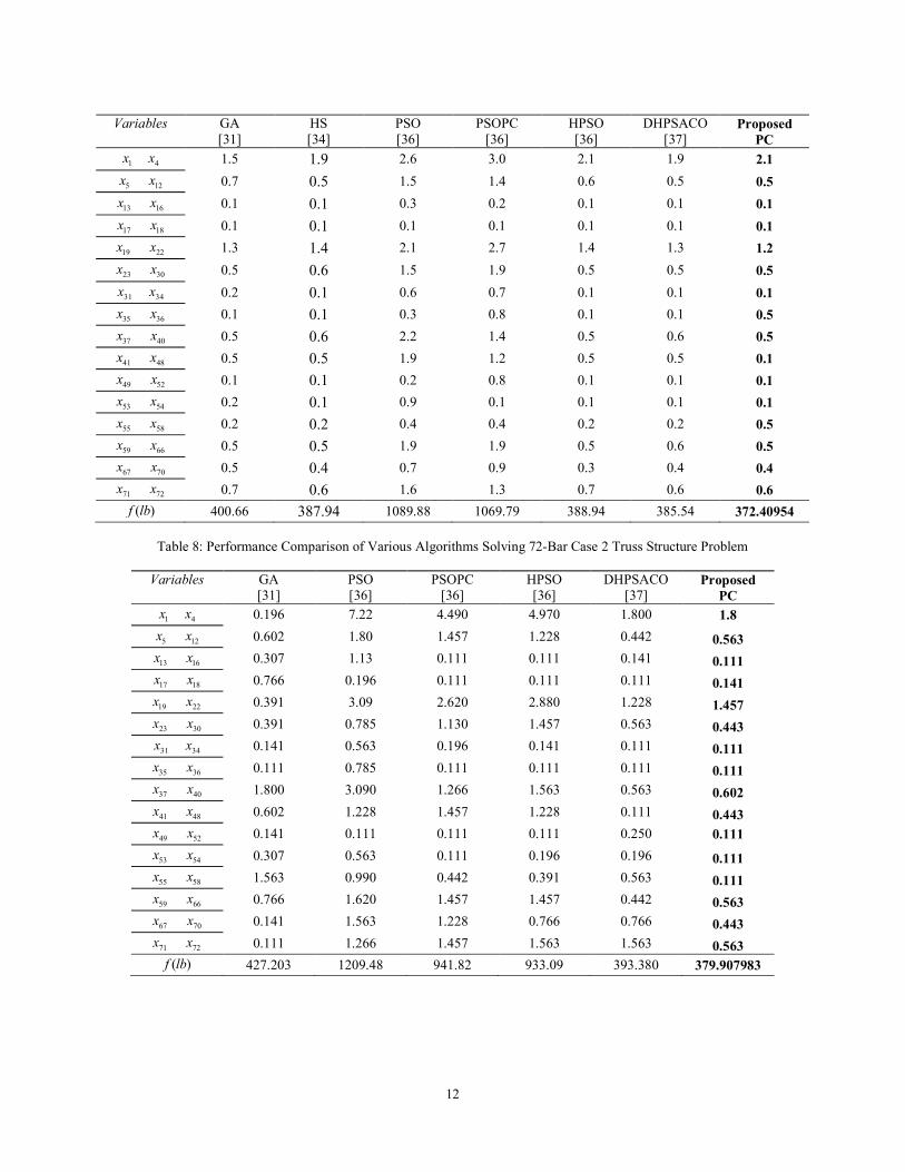
This problem was previously solved in [31, 34, 36, 37]. The best results obtained using these approaches along

with PC methodology for Case 1 and Case 2 are listed in Table 7 and Table 8, respectively. The PC solution to the

problem produced competent results at reasonable computational cost. The best, mean and worst function values,

i.e. the weight W of the truss structure for Case 1 obtained from twenty trials were 372.40954 lb, 380.10692 lb

and 395.99776 lb with standard deviation of 6.757504 and for Case 2 were 379.907983 lb, 382.329656 lb and

383.857921 lb, respectively with standard deviation 1.369460465. The average CPU time, average number of

function evaluations and associated parameters are listed in Table 9. The convergence plots for Case 1 and Case 2

are shown in Figure 8 and Figure 9, respectively.

Table 6: Loading Condition for 72 Bar

Nodes xP yP kips

zP xP yP zP kips

17 5.0 5.0 0.0 0.0 0.0 -5.0

18 0.0 0.0 0.0 0.0 0.0 -5.0

19 0.0 0.0 0.0 0.0 0.0 -5.0

20 0.0 0.0 0.0 0.0 0.0 -5.0

Table 7: Performance Comparison of Various Algorithms Solving 72-Bar Case 1 Truss Structure Problem

12

Variables GA

[31]

HS

[34]

PSO

[36]

PSOPC

[36]

HPSO

[36]

DHPSACO

[37] Proposed

PC

1 4x x� 1.5 1.9 2.6 3.0 2.1 1.9 2.1

5 12 x x� 0.7 0.5 1.5 1.4 0.6 0.5 0.5

13 16 x x� 0.1 0.1 0.3 0.2 0.1 0.1 0.1

17 18 x x� 0.1 0.1 0.1 0.1 0.1 0.1 0.1

19 22 x x� 1.3 1.4 2.1 2.7 1.4 1.3 1.2

23 30 x x� 0.5 0.6 1.5 1.9 0.5 0.5 0.5

31 34x x� 0.2 0.1 0.6 0.7 0.1 0.1 0.1

35 36 x x� 0.1 0.1 0.3 0.8 0.1 0.1 0.5

37 40 x x� 0.5 0.6 2.2 1.4 0.5 0.6 0.5

41 48 x x� 0.5 0.5 1.9 1.2 0.5 0.5 0.1

49 52 x x� 0.1 0.1 0.2 0.8 0.1 0.1 0.1

53 54 x x� 0.2 0.1 0.9 0.1 0.1 0.1 0.1

55 58 x x� 0.2 0.2 0.4 0.4 0.2 0.2 0.5

59 66 x x� 0.5 0.5 1.9 1.9 0.5 0.6 0.5

67 70 x x� 0.5 0.4 0.7 0.9 0.3 0.4 0.4

71 72 x x� 0.7 0.6 1.6 1.3 0.7 0.6 0.6

( )f lb 400.66 387.94 1089.88 1069.79 388.94 385.54 372.40954

Table 8: Performance Comparison of Various Algorithms Solving 72-Bar Case 2 Truss Structure Problem

Variables GA

[31]

PSO

[36]

PSOPC

[36]

HPSO

[36]

DHPSACO

[37] Proposed

PC

1 4x x� 0.196 7.22 4.490 4.970 1.800 1.8

5 12 x x� 0.602 1.80 1.457 1.228 0.442 0.563

13 16 x x� 0.307 1.13 0.111 0.111 0.141 0.111

17 18 x x� 0.766 0.196 0.111 0.111 0.111 0.141

19 22 x x� 0.391 3.09 2.620 2.880 1.228 1.457

23 30 x x� 0.391 0.785 1.130 1.457 0.563 0.443

31 34x x� 0.141 0.563 0.196 0.141 0.111 0.111

35 36 x x� 0.111 0.785 0.111 0.111 0.111 0.111

37 40 x x� 1.800 3.090 1.266 1.563 0.563 0.602

41 48 x x� 0.602 1.228 1.457 1.228 0.111 0.443

49 52 x x� 0.141 0.111 0.111 0.111 0.250 0.111

53 54 x x� 0.307 0.563 0.111 0.196 0.196 0.111

55 58 x x� 1.563 0.990 0.442 0.391 0.563 0.111

59 66 x x� 0.766 1.620 1.457 1.457 0.442 0.563

67 70 x x� 0.141 1.563 1.228 0.766 0.766 0.443

71 72 x x� 0.111 1.266 1.457 1.563 1.563 0.563

( )f lb 427.203 1209.48 941.82 933.09 393.380 379.907983

13

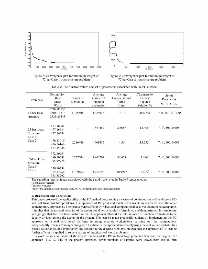
Figure 8: Convergence plot for minimum weight of

72-bar Case 1 truss structure problem

Figure 9: Convergence plot for minimum weight of

72-bar Case 2 truss structure problem

Table 9: The function values and set of parameters associated with the PC method

Problems

System Sol.

Best

Mean

Worst

Standard

Deviation

Average

number of

function

evaluation

Average

Computational

Time

(min.)

Closeness to

the best

Reputed

Solution %

Set of

Parameters

im λ T Tα

17-bar truss

structure

2584.02556

2586.11318

2589.25345

1.375508

6628943

18.78

-0.04551

7, 0.001c, 40, 0.05

25-bar truss

Structure

Case 1

Case 2

477.16684

477.16684

477.16684

476.43010

476.56160

477.15846

0

0.216449

1844457

1963415

2.3657

4.56

13.495*

13.555*

7, 1d, 500, 0.005

7, 1d, 500, 0.005

72-Bar Truss

Structure

Case 1

Case 2

372.40954

380.10692

395.99776

379.90798

382.32966

383.85792

6.757504

1.369460

8843207

8730598

34.458

30.9947

3.424*

3.405*

7, 1d, 500, 0.005

7, 1d, 500, 0.005

The sampling interval factor associated with the c and d are listed in Table 9 represented as: c Continuous Variable d Discrete Variable

*Shows the optimal design obtained using PC was better than the associated algorithms.

6. Discussion and Conclusion This paper proposed the applicability of the PC methodology solving a variety of continuous as well as discrete 2-D

and 3-D truss structure problems. The approach of PC produced much better results as compared with the other

contemporary approaches. The results were sufficiently robust and computational cost was found to be acceptable.

It implies that the rational behavior of the agents could be successfully formulated and demonstrated. It is important

to highlight that the distributed nature of the PC approach allowed the total number of function evaluations to be

equally divided among the agents of the system. This can be made practically evident by implementing the PC

approach on a real distributed platform assigning separate workstations carrying out the computations

independently. These advantages along with the directly incorporated uncertainty using the real valued probabilities

treated as variables, and importantly, the solution to the discrete problems indicate that the approach of PC can be

further efficiently applied to solve a variety of practical/real world problems.

It is worth to mention some of the key differences of the PC methodology presented here and the original PC

approach [1-3, 12, 14]. In the present approach, fewer numbers of samples were drawn from the uniform

0 1000 2000 3000 4000 5000 6000 7000 8000 9000 10000300

400

500

600

700

800

900

1000

1100

1200

Iterations

Truss Weight 'f' lb

0 2000 4000 6000 8000 100000

1000

2000

3000

4000

5000

Iterations

Truss Weight 'f' lb

14

distribution of the individual agent’s sampling interval. On the contrary, the original PC approach used a Monte

Carlo sampling method which was computationally expensive and slow as the number of samples needed was in the

thousands or even millions. Most significantly, the sampling in further stages of the PC algorithm presented here

was narrowed down in every iteration by selecting the sampling interval in the neighborhood of the most favorable

value in the particular iteration. This ensures faster convergence and an improvement in efficiency over the original

PC approach in which regression was necessary to sample the strategy values in the close neighborhood of the

favorable value. Moreover, the coordination among the agents representing the variables in the system was achieved

based on the partial small bit of information. In other words, in order to optimize the global/system objective every

agent selects its best possible strategy by guessing the model of every other agent based merely on their recent

favorable strategies communicated. This gives the advantage to the agents and the entire system to quickly search

the better solution and reach the Nash equilibrium and avoid the tragedy of commons [5, 6]. The work on fine tuning

the parameters such as the number of strategies im in every agent’s strategy set

iX and the interval factor λ which

essentially decide the rate of solution convergence is currently underway.

7. References [1] D.H. Wolpert, Information Theory-The Bridge Connecting Bounded Rational Game Theory and Statistical

Physics, In: D. Braha, A.A. Minai, Y. Bar-Yam (Eds.), Complex Engineered Systems, Springer, 262-290,

2006.

[2] D.H. Wolpert and K. Tumer, An Introduction to Collective Intelligence, Technical Report, NASA

ARC-IC-99-63, NASA Ames Research Center, 1999.

[3] S.R. Bieniawski, Distributed Optimization and Flight Control Using Collectives, PhD Dissertation, Stanford

University, 2005.

[4] A.J. Kulkarni and K. Tai, Probability Collectives: A Multi-Agent Approach for Solving Combinatorial

Optimization Problems, Applied Soft Computing, 10 (3), 759–771, 2010.

[5] A.J. Kulkarni and K. Tai, A Probability Collectives Approach with a Feasibility-Based Rule for Constrained

Optimization, Applied Computational Intelligence and Soft Computing, Article ID 980216, 2011.

[6] A.J. Kulkarni and K. Tai, Probability Collectives: A Decentralized, Distributed Optimization for

Multi-Agent Systems, In: Application of Soft Computing, J. Mehnen, M. Koeppen, A.Saad, A. Tiwari (Eds.),

Springer, 58, 441-450, 2009.

[7] A.J. Kulkarni and K. Tai, Probability Collectives: A Distributed Optimization Approach for Constrained

Problems, Proc. IEEE World Congress on Computational Intelligence, 18-23, 2010.

[8] A.J. Kulkarni and K. Tai, Probability Collectives for Decentralized, Distributed Optimization: A Collective

Intelligence Approach, Proc. IEEE International Conferrnce on System, Man and Cybernetics, 1271-1275,

2008.

[9] A.J. Kulkarni and K. Tai, Solving Consrained Optimization problem Using Probability Collectives and a

Penalty Function Approach, International Journal of Computational Intelligence and Application, 10 (4),

445-470, 2011.

[10] A.J. Kulkarni and K. Tai, Solving Sensor Network Coverage Problems Using a Constrained Probability

Collectives Approach, (Submitted to Computational Intelligence), August 2013.

[11] A.J. Kulkarni and K. Tai, A Probability Collectives Approach for Multi-Agent Distributed and Cooperative

Optimization with Tolerance for Agent Failure, In: Agent Based Optimization, I. Czarnowski et al. (Eds.),

Springer-Verlag, 175-201, 2012.

[12] D.H. Wolpert, N.E. Antoine and S.R. Bieniawski and I.R. Kroo, Fleet Assignment using Collective

Intelligence, Proc. 42nd AIAA Aerospace Science Meeting Exhibit, 2004.

[13] A.J. Kulkarni, N.S. Patankar, A. Sandupatla and K. Tai, A Modified Feasibility-based Rule for Solving

Constrained Optimization Problem using probability Collectives, Proc. IEEE 12th International Conferrence

of Hybrid Intelligence System (HIS), 213-218, 2012.

[14] S. Bieniawski, D. Wolpert and I. Kroo, Discrete, Continuous, and Constrained Optimization using

Collectives, Proc. 10th AIAA/ISSMO Multidisciplinary Analysis and Optimization Conference, AIAA Paper,

2004-4580, 2004.

[15] A.J. Kulkarni, I.R.Kale, K.Tai and S.K. Azad, “Discrete Optimization of Truss Structure using Probability

Collectives, Proc. IEEE 12th International Conferrence of Hybrid Intelligence System (HIS), 225-230, 2012.

[16] B. Autry, University Course Timetabling with Probability Collectives, Master’s Thesis, Naval Postgraduate

School Montery, 2008.

15

[17] S. Bhadra, S. Shakkotai and P. Gupta, Min-Cost Selfish Multicast with Network Coding, Proc. IEEE

Transactions on Information Theory, 52 (11), 5077-5087, 2006.

[18] Y. Xi and E.M. Yeh, Distributed algorithms for minimum cost multicast with network coding in wireless

networks, Proc. 4th International Symposium on Modeling and Optimization in Mobile, Ad Hoc and Wireless

Networks, 2006.

[19] J. Yuan, Z. Li, W. Yu and B. Li, A Cross-layer Optimization Framework for Multicast in Multi-Hop Wireless

Networks, Proc. 1st International Conference on Wireless Internet, 47-54, 2005.

[20] M. Chatterjee, S. Sas and K.D. Turgut, An On-demand Weighted Clustering Algorithm (WCA) for Ad Hoc

Networks, Proc. 43rd IEEE Global Telecommunications Conference, 1697-1701, 2000.

[21] M.H. Amerimehr, B.K. Khalaj and P.M. Crespo, A Distributed Cross-layer Optimization Method for

Multicast in Interference-Limited Multihop Wireless Networks, Journal on Wireless Communications and

Networking, 2008, Article ID 702036.

[22] H.A. Mohammad and H.K. Babak, A Distributed Probability Collectives Optimization Method for Multicast

in CDMA Wireless Data Networks, Proc. 4th IEEE Internatilonal Symposium on Wireless Communication

Systems, 617-621, 2007.

[23] M. Smyrnakis and D.S. Leslie, Sequentially Updated Probability Collectives, Proc. 48th IEEE Conference on

Decision and Control and 28th Chinese Control Conference, 5774-5779, 2009.

[24] C.F. Huang, S. Bieniawski, D. Wolpert and C.E.M.A. Strauss, Comparative Study of Probability Collectives

based Multiagent Systems and Genetic Algorithms, Proc. Conference on Genetic and Evolutionary

Computation, 751–752, 2005.

[25] M. Vasirani and S. Ossowski, Collective-based Multiagent Coordination, LNAI 4995, 240-253, 2008.

[26] M. Bowling and M. Veloso, Rational and Convergent Learning in Stochastic Games, Proc. 17th International

Conference on Artificial Intelligence, 1021–1026, 2001.

[27] V. Sindhwani, S.S. Keerthi and O. Chapelle, Deterministic Annealing for Semi-supervised Kernel Machines,

Proc. 23rd International Conference on Machine Learning, 2006.

[28] A.V. Rao, D.J. Miller, K. Rose and A. Gersho, A Deterministic Annealing Approach for Parsimonious

Design of Piecewise Regression Models, Proc. IEEE Transactions on Patternt Analysis and Machine

Intelligence, 21 (2), 159-173, 1999.

[29] A.V. Rao, D.J. Miller, K. Rose and A. Gersho, Mixture of Experts Regression Modeling by Deterministic

Annealing, Proc. IEEE Transactions on Signal Processing, 45 (11), 2811-2820, 1997.

[30] R. Czabanski, Deterministic Annealing Integrated with Intensive Learning in Neuro-fuzzy Systems, LNAI

4029, 220-229, 2006.

[31] S.J. Wu and P.T. Chow, Steady-state Genetic Algorithms for Discrete Optimization of Trusses, Computers

and Structures, 56 (6), 979-991, 1994.

[32] H. Adeli and S. Kumar, Distributed Genetic Algorithm for Structural Optimization, Journal of Aerospace

Engineering, ASCE, 8 (3), 156-163, 1995.

[33] K.S. Lee and Z.W. Geem, A New Structural Optimization Method Based on the Harmony Search

Algorithm, Computers Structures, 82, 781-798, 2004.

[34] K.S. Lee, Z.W. Geem, S.H. Lee and K.W. Bae, The Harmony Search Heuristic Algorithm for Discrete

Structural Optimization, Engineering Optimization, 37 (7), 663-684, 2005.

[35] L.J. Li, Z.B. Huang, F. Liu and Q.H. Wu, A Heuristic Particle Swarm Optimization of Pin Connected

Structures, Computers and Structures, 85, 340-349, 2007.

[36] L.J. Li, Z.B. Huang and F. Liu, A Heuristic Particle Swarm Optimization Method for Truss Structures with

Discrete Variables, Computers and Structures, 87 (7-8), 435-443, 2009.

[37] A. Kaveh and S. Talatahari, A Particle Swarm Ant Colony Optimization for Truss Structures with Discrete

Variables, Journal of Structural Steel Research, 65, 1558-1568, 2009.