Embed Size (px)
Citation preview
2
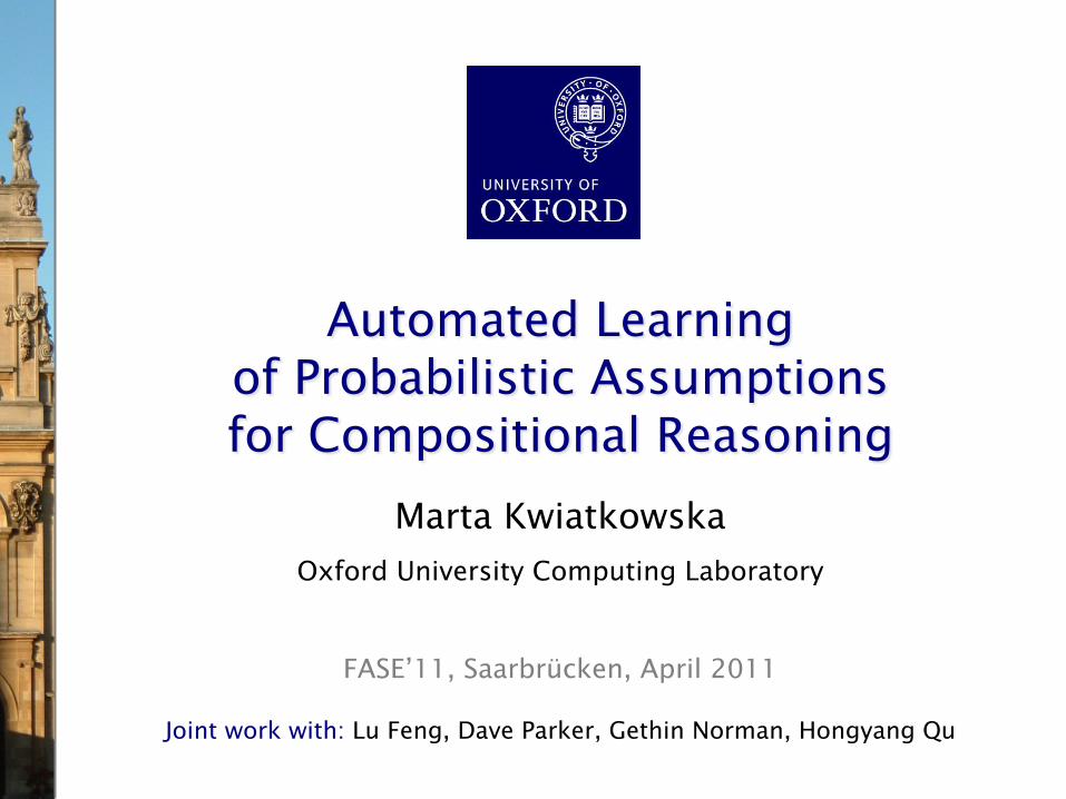
Probabilistic verification
• Probabilistic verification − formal verification of systems exhibiting stochastic behaviour
• Why probability? − unreliability (e.g. component failures) − uncertainty (e.g. message losses/delays over wireless) − randomisation (e.g. in protocols such as Bluetooth, ZigBee)
• Quantitative properties − reliability, performance, quality of service, … − “the probability of an airbag failing to deploy within 0.02s” − “the expected time for a network protocol to send a packet” − “the expected power usage of a sensor network over 1 hour”
3
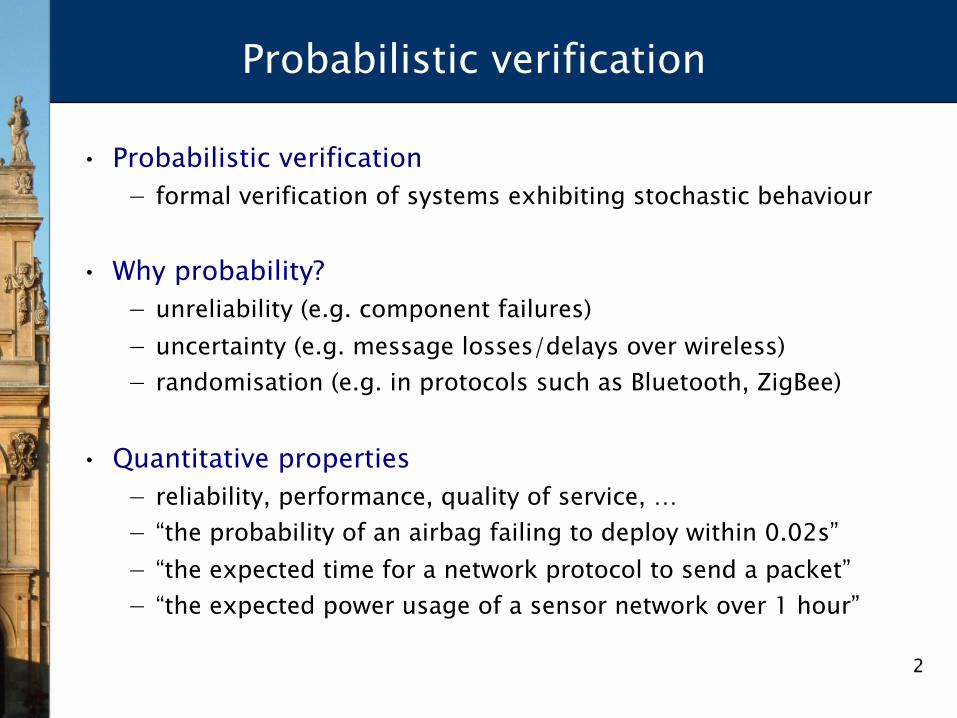
Model checking
Automated formal verification for finite-state models
Finite-state model
Temporal logic specification
Result System
Counter- example
System require-
ments
¬EF fail
Model checker e.g. SMV, Spin
4
Probabilistic model checking
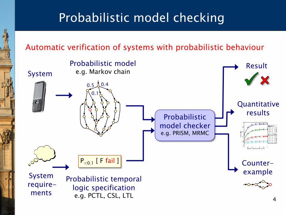
Automatic verification of systems with probabilistic behaviour
Probabilistic model e.g. Markov chain
Probabilistic temporal logic specification e.g. PCTL, CSL, LTL
Result
Quantitative results
System
Counter- example System
require- ments
P<0.1 [ F fail ]
0.5 0.1
0.4
Probabilistic model checker e.g. PRISM, MRMC
5
Probabilistic model checking
• First algorithms proposed in 1980s − [Vardi, Courcoubetis, Yannakakis, …] − algorithms [Hansson, Jonsson, de Alfaro] & first implementations
• 2000: tools ETMCC (MRMC) & PRISM released − PRISM: efficient extensions of symbolic model checking − ETMCC (now MRMC): model checking for continuous-time Markov
chains [Baier, Hermanns, Haverkort, Katoen, …]
• Selected advances in probabilistic model checking: − compositional verification [Segala, Lynch, Stoelinga, Vaandrager, …] − probabilistic counterexample generation [Han/Katoen, Leue, …] − abstraction (and CEGAR) for probabilistic models
• [Larsen, Hermanns, Wolf, Kwiatkowska, ... ] − and much more…
6
Probabilistic model checking in action
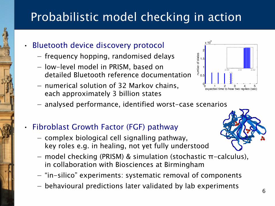
• Bluetooth device discovery protocol − frequency hopping, randomised delays − low-level model in PRISM, based on
detailed Bluetooth reference documentation − numerical solution of 32 Markov chains,
each approximately 3 billion states − analysed performance, identified worst-case scenarios
• Fibroblast Growth Factor (FGF) pathway − complex biological cell signalling pathway,
key roles e.g. in healing, not yet fully understood − model checking (PRISM) & simulation (stochastic π-calculus),
in collaboration with Biosciences at Birmingham − “in-silico” experiments: systematic removal of components − behavioural predictions later validated by lab experiments
7
Probabilistic model checking
• What’s involved − specifying, constructing probabilistic models − graph-based analysis: reachability + qualitative verification − numerical solution, e.g. linear equations/linear programming
• The state of the art − fast/efficient techniques for a range of probabilistic models − (mostly Markov chains, Markov decision processes) − feasible for models of up to 107 states (1010 with symbolic) − tool support exists and is widely used, e.g. PRISM, MRMC − successfully applied to many application domains:
• distributed randomised algorithms, communication protocols, security protocols, biological systems, quantum cryptography, …
8
Probabilistic model checking
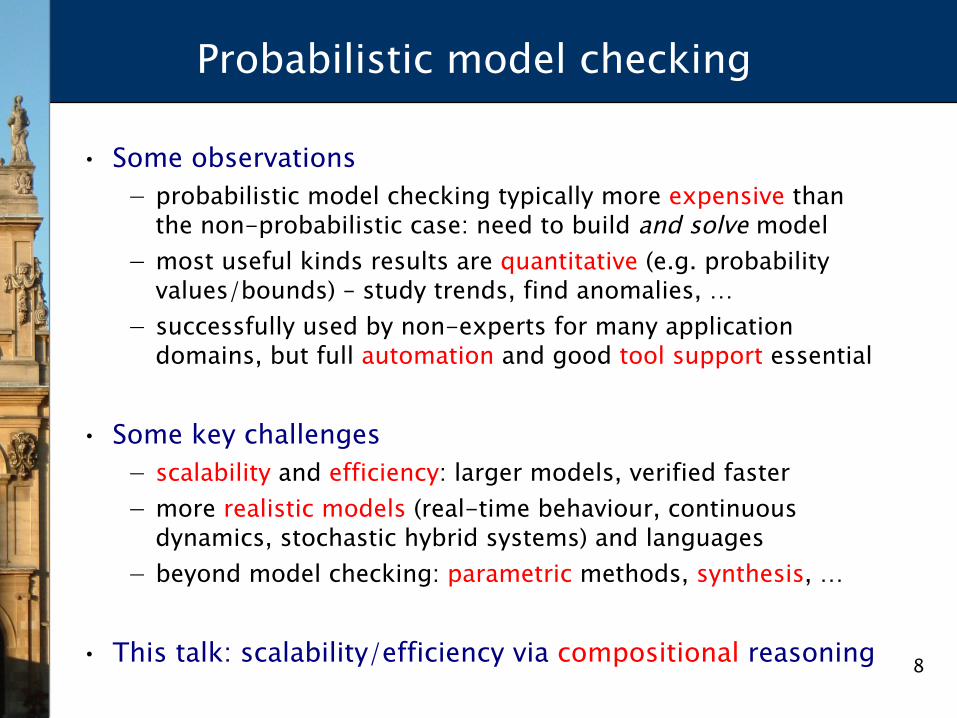
• Some observations − probabilistic model checking typically more expensive than
the non-probabilistic case: need to build and solve model − most useful kinds results are quantitative (e.g. probability
values/bounds) – study trends, find anomalies, … − successfully used by non-experts for many application
domains, but full automation and good tool support essential
• Some key challenges − scalability and efficiency: larger models, verified faster − more realistic models (real-time behaviour, continuous
dynamics, stochastic hybrid systems) and languages − beyond model checking: parametric methods, synthesis, …
• This talk: scalability/efficiency via compositional reasoning
9
Overview
• Probabilistic model checking − probabilistic models: probabilistic automata − property specifications: probabilistic safety properties − multi-objective model checking
• Compositional probabilistic verification − assume-guarantee reasoning − assume-guarantee for probabilistic systems − implementation & results
• Automated generation of assumptions − L* and its application to compositional verification − generating probabilistic assumptions − implementation, results & recent progress
• Conclusions
10
Probabilistic models
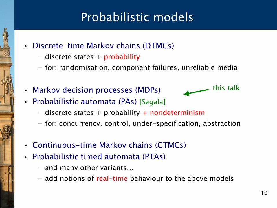
• Discrete-time Markov chains (DTMCs) − discrete states + probability − for: randomisation, component failures, unreliable media
• Markov decision processes (MDPs) • Probabilistic automata (PAs) [Segala]
− discrete states + probability + nondeterminism − for: concurrency, control, under-specification, abstraction
• Continuous-time Markov chains (CTMCs) • Probabilistic timed automata (PTAs)
− and many other variants… − add notions of real-time behaviour to the above models
this talk
11
Probabilistic automata (PAs)
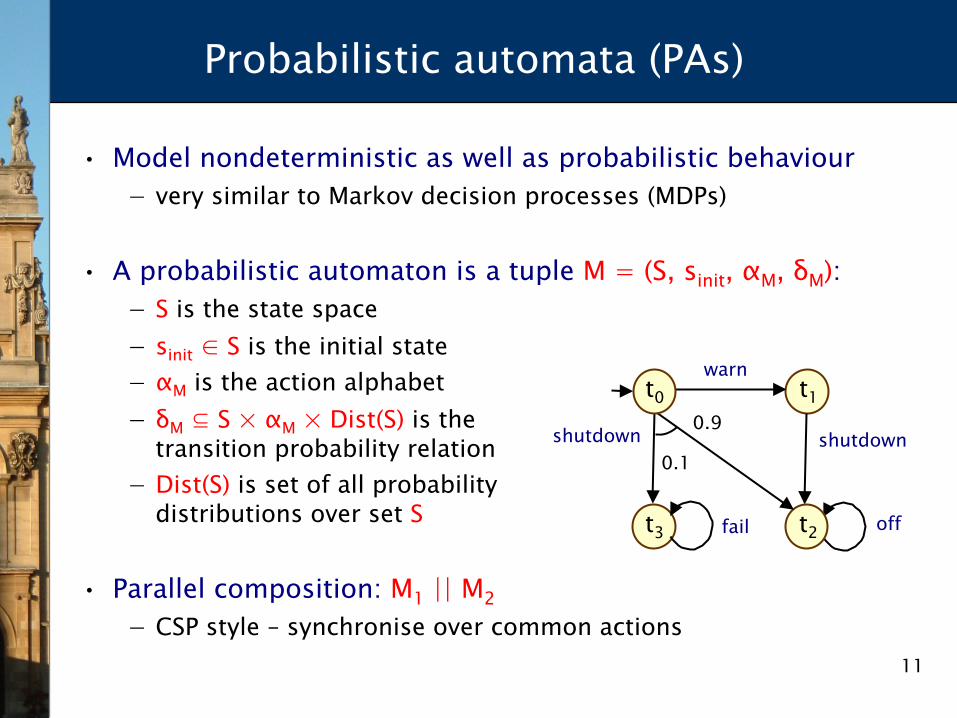
• Model nondeterministic as well as probabilistic behaviour − very similar to Markov decision processes (MDPs)
• A probabilistic automaton is a tuple M = (S, sinit, αM, δM): − S is the state space − sinit ∈ S is the initial state − αM is the action alphabet − δM ⊆ S × αM × Dist(S) is the
transition probability relation − Dist(S) is set of all probability
distributions over set S
• Parallel composition: M1 || M2 − CSP style – synchronise over common actions
t1
0.1
warn
t2 t3
shutdown 0.9 shutdown
t0
fail off
12
Probabilistic model checking for PAs
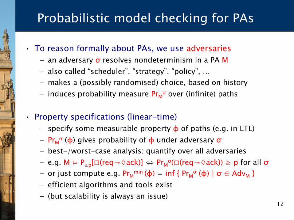
• To reason formally about PAs, we use adversaries − an adversary σ resolves nondeterminism in a PA M − also called “scheduler”, “strategy”, “policy”, … − makes a (possibly randomised) choice, based on history − induces probability measure PrM
σ over (infinite) paths
• Property specifications (linear-time) − specify some measurable property φ of paths (e.g. in LTL) − PrM
σ (φ) gives probability of φ under adversary σ − best-/worst-case analysis: quantify over all adversaries − e.g. M ⊨ P≥p[□(req→◊ack)] ⇔ PrM
σ(□(req→◊ack)) ≥ p for all σ − or just compute e.g. PrM
min (φ) = inf { PrMσ (φ) | σ ∈ AdvM }
− efficient algorithms and tools exist − (but scalability is always an issue)
13
Running example
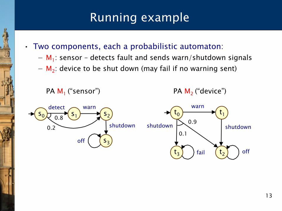
• Two components, each a probabilistic automaton: − M1: sensor – detects fault and sends warn/shutdown signals − M2: device to be shut down (may fail if no warning sent)
PA M2 (“device”) PA M1 (“sensor”)
t1
0.1
warn
t2 t3
shutdown 0.9 shutdown
t0
fail off
s0
0.2
detect
s3
s1 0.8 shutdown
warn
off
s2
14
Running example
s0,t0
0.2
detect 0.8
warn s1,t0
s2,t0
s2,t1
shutdown
0.1
shutdown
0.9 s1,t2
s2,t3
off
fail
s3,t2 off
PA M2 (“device”) PA M1 (“sensor”)
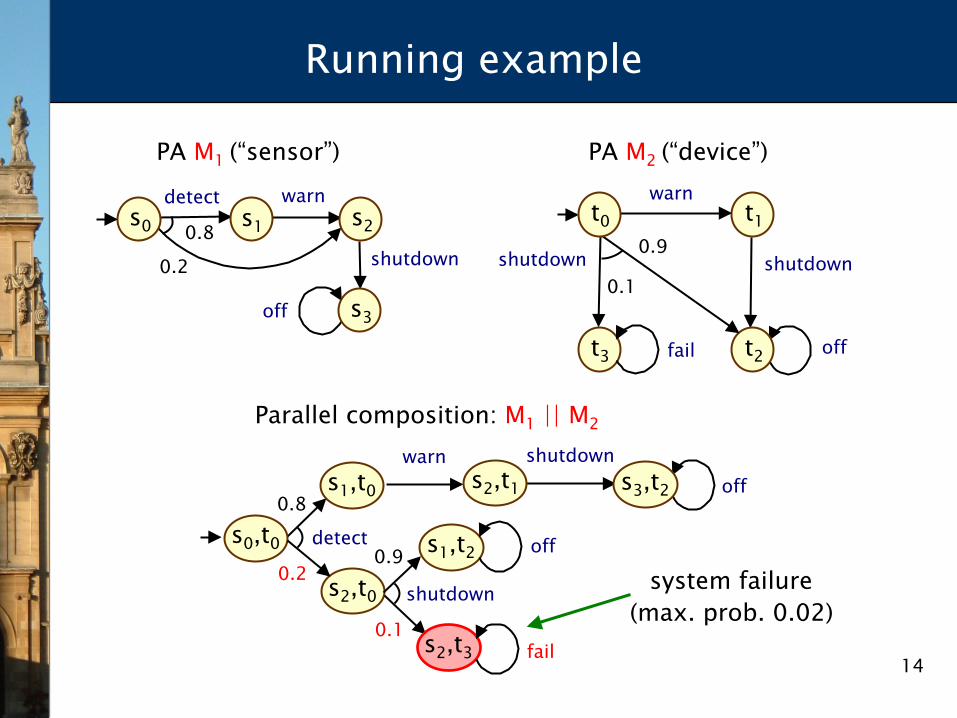
Parallel composition: M1 || M2
system failure (max. prob. 0.02)
t1
0.1
warn
t2 t3
shutdown 0.9 shutdown
t0
fail off
s0
0.2
detect
s3
s1 0.8 shutdown
warn
off
s2
15
Safety properties
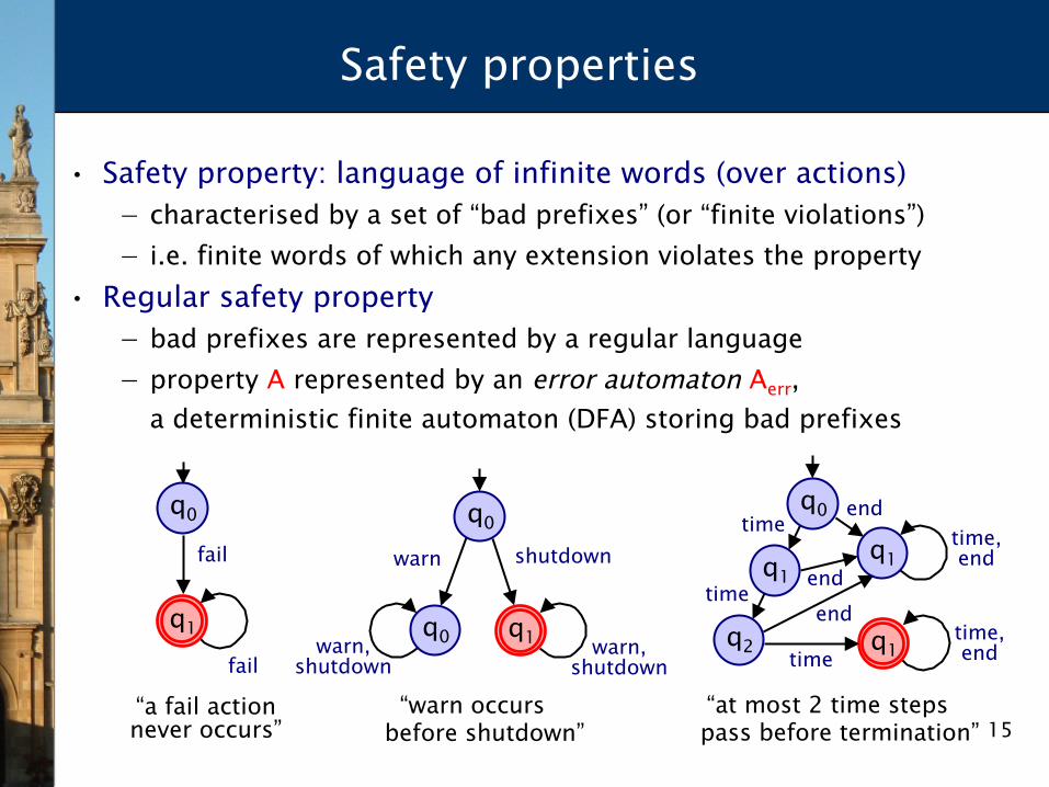
• Safety property: language of infinite words (over actions) − characterised by a set of “bad prefixes” (or “finite violations”) − i.e. finite words of which any extension violates the property
• Regular safety property − bad prefixes are represented by a regular language − property A represented by an error automaton Aerr,
a deterministic finite automaton (DFA) storing bad prefixes
“a fail actionnever occurs”
“warn occursbefore shutdown”
“at most 2 time stepspass before termination”
fail
fail
q0
q1
shutdown warn
q0
q1 q0 warn, shutdown
warn, shutdown
time time, end
q0
q1
q1 time
q2 time
q1
end
end end
time, end
16
Probabilistic safety properties
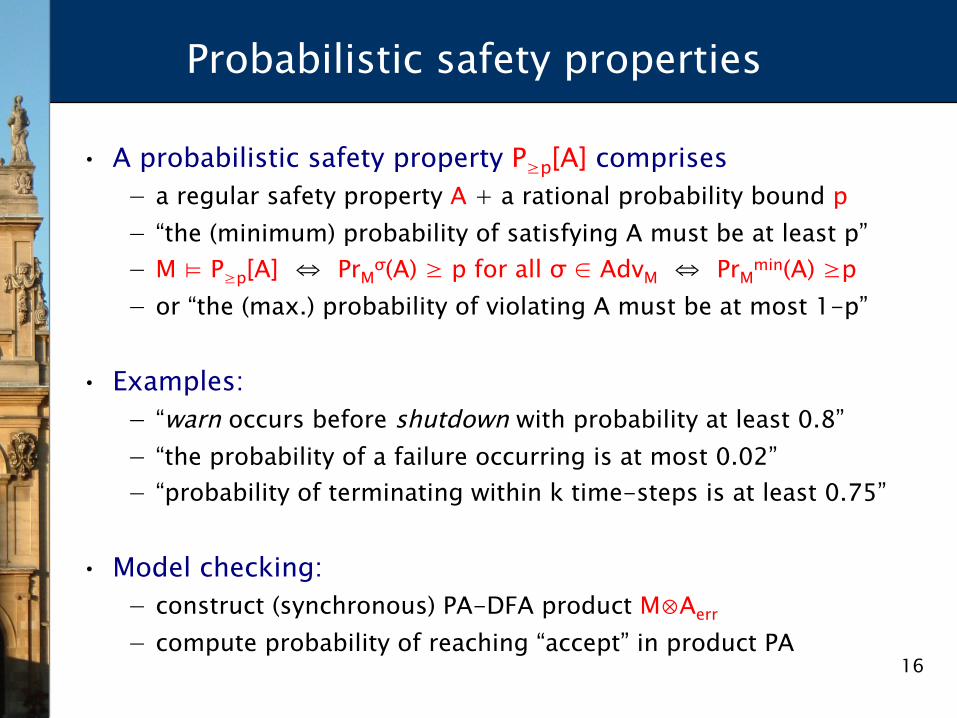
• A probabilistic safety property P≥p[A] comprises − a regular safety property A + a rational probability bound p − “the (minimum) probability of satisfying A must be at least p” − M ⊨ P≥p[A] ⇔ PrM
σ(A) ≥ p for all σ ∈ AdvM ⇔ PrMmin(A) ≥p
− or “the (max.) probability of violating A must be at most 1-p”
• Examples: − “warn occurs before shutdown with probability at least 0.8” − “the probability of a failure occurring is at most 0.02” − “probability of terminating within k time-steps is at least 0.75”
• Model checking: − construct (synchronous) PA-DFA product M⊗Aerr − compute probability of reaching “accept” in product PA
17
Running example
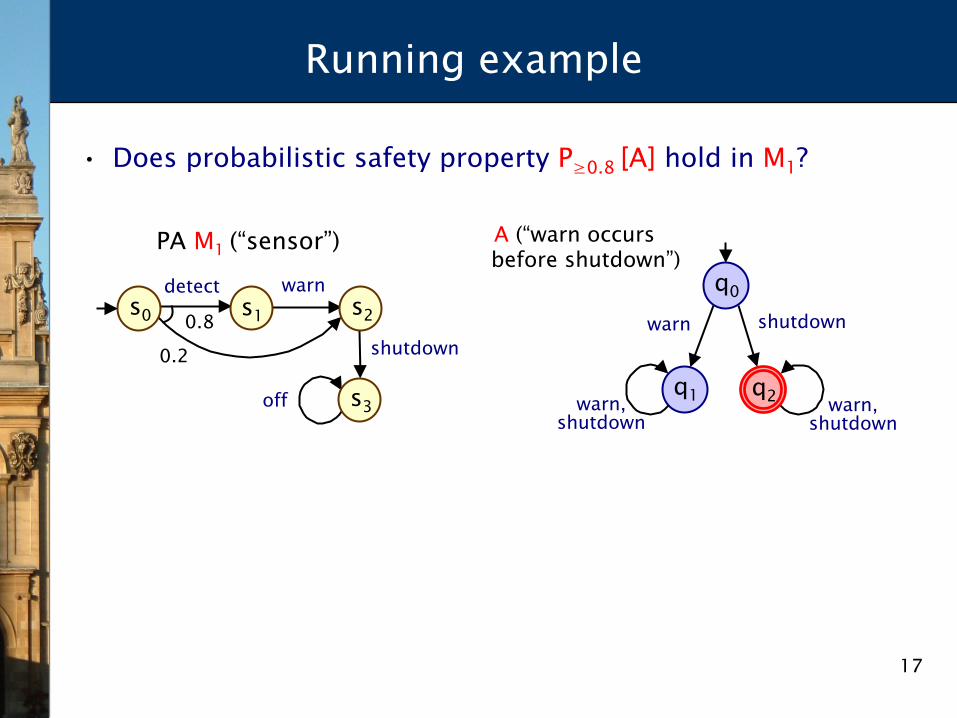
• Does probabilistic safety property P≥0.8 [A] hold in M1?
PA M1 (“sensor”)
s0
0.2
detect
s3
s1 0.8 shutdown
warn
off
s2
A (“warn occursbefore shutdown”)
shutdown warn
q0
q2 q1 warn, shutdown
warn, shutdown

18
Running example
• Does probabilistic safety property P≥0.8 [A] hold in M1?
PA M1 (“sensor”)
s0
0.2
detect
s3
s1 0.8 shutdown
warn
off
s2
A (“warn occursbefore shutdown”)
shutdown warn
q0
q2 q1 warn, shutdown
warn, shutdown
Product PA M1⊗Aerr
s0,q0
0.2 detect
0.8
shutdown
warn s1,q0
s2,q0
s2,q1 s3,q1
shutdown
off
off
s3,q2
PrM1min(A)
= 1 – 0.2 = 0.8 → M1 ⊨ P≥0.8 [A]
19
Multi-objective PA model checking
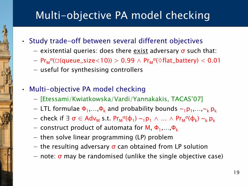
• Study trade-off between several different objectives − existential queries: does there exist adversary σ such that: − PrM
σ(□(queue_size<10)) > 0.99 ∧ PrMσ(◊flat_battery) < 0.01
− useful for synthesising controllers
• Multi-objective PA model checking − [Etessami/Kwiatkowska/Vardi/Yannakakis, TACAS’07] − LTL formulae Φ1,…,Φk and probability bounds ~1p1,…,~k pk
− check if ∃ σ ∈ AdvM s.t. PrMσ(φ1) ~1p1 ∧ … ∧ PrM
σ(φk) ~k pk − construct product of automata for M, Φ1,…,Φk − then solve linear programming (LP) problem − the resulting adversary σ can obtained from LP solution − note: σ may be randomised (unlike the single objective case)
20
Multi-objective PA model checking
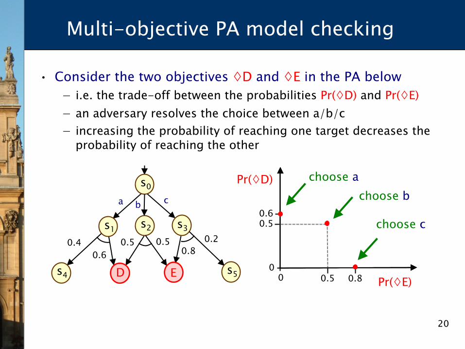
• Consider the two objectives ◊D and ◊E in the PA below − i.e. the trade-off between the probabilities Pr(◊D) and Pr(◊E) − an adversary resolves the choice between a/b/c − increasing the probability of reaching one target decreases the
probability of reaching the other
c a
s0
s3 s2
b
0.4 0.6
0.5 0.5 0.8
0.2
s5 E D
s1
s4
choose a Pr(◊D)
Pr(◊E) 0.8 0.5
0.5 0.6
0 0
choose b
choose c
21
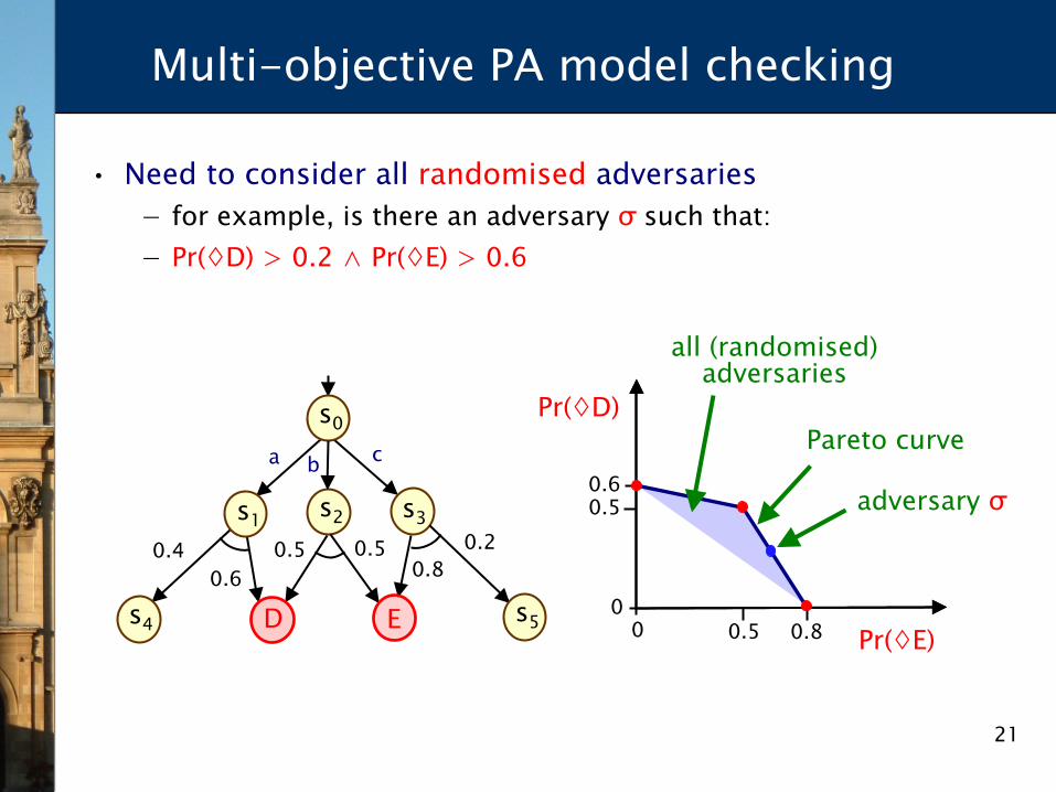
Multi-objective PA model checking
• Need to consider all randomised adversaries − for example, is there an adversary σ such that: − Pr(◊D) > 0.2 ∧ Pr(◊E) > 0.6
c a
s0
s3 s2
b
0.4 0.6
0.5 0.5 0.8
0.2
s5 E D
s1
s4
Pr(◊D)
Pr(◊E) 0.8 0.5
0.5 0.6
0 0
all (randomised) adversaries
Pareto curve
adversary σ
22
Overview
• Probabilistic model checking − probabilistic automata − property specification + probabilistic safety properties − multi-objective model checking
• Compositional probabilistic verification − assume-guarantee reasoning − assume-guarantee for probabilistic systems − implementation & results
• Automated generation of assumptions − L* and its application to compositional verification − generating probabilistic assumptions − implementation & results
• Conclusions, current & future work
23
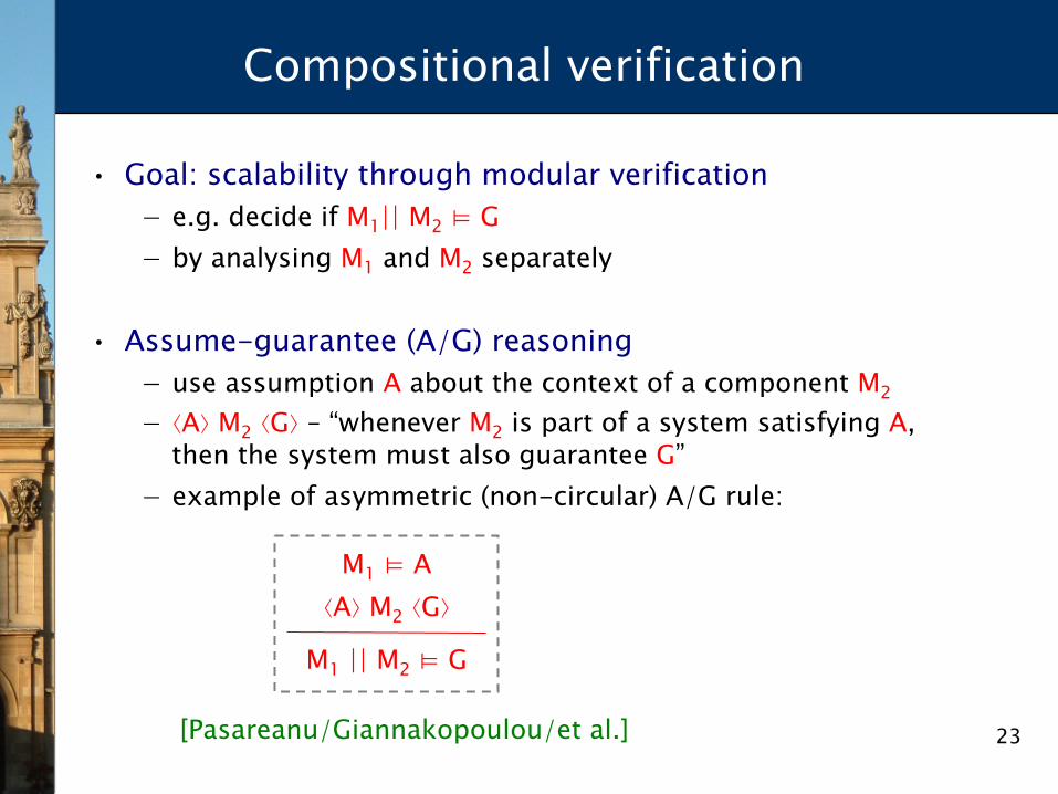
Compositional verification
• Goal: scalability through modular verification − e.g. decide if M1|| M2 ⊨ G − by analysing M1 and M2 separately
• Assume-guarantee (A/G) reasoning − use assumption A about the context of a component M2
− ⟨A⟩ M2 ⟨G⟩ – “whenever M2 is part of a system satisfying A, then the system must also guarantee G”
− example of asymmetric (non-circular) A/G rule:
[Pasareanu/Giannakopoulou/et al.]
M1 ⊨ A
⟨A⟩ M2 ⟨G⟩
M1 || M2 ⊨ G
24
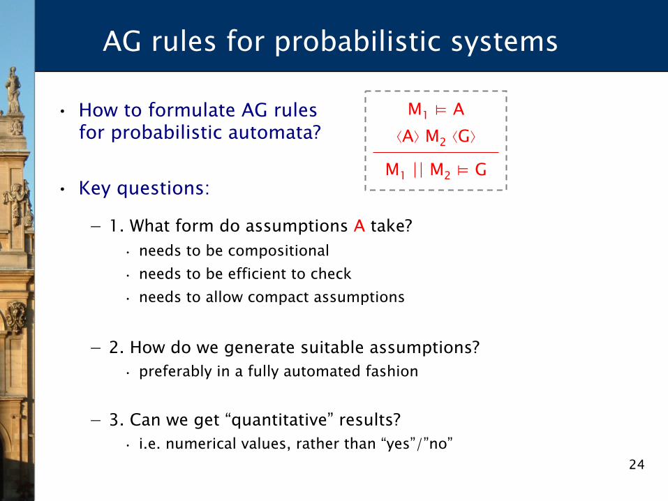
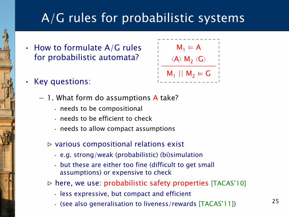
AG rules for probabilistic systems
• How to formulate AG rulesfor probabilistic automata?
• Key questions:
− 1. What form do assumptions A take? • needs to be compositional • needs to be efficient to check • needs to allow compact assumptions
− 2. How do we generate suitable assumptions? • preferably in a fully automated fashion
− 3. Can we get “quantitative” results? • i.e. numerical values, rather than “yes”/”no”
M1 ⊨ A
⟨A⟩ M2 ⟨G⟩
M1 || M2 ⊨ G
25
A/G rules for probabilistic systems
• How to formulate A/G rulesfor probabilistic automata?
• Key questions:
− 1. What form do assumptions A take? • needs to be compositional • needs to be efficient to check • needs to allow compact assumptions
▷ various compositional relations exist • e.g. strong/weak (probabilistic) (bi)simulation • but these are either too fine (difficult to get small
assumptions) or expensive to check ▷ here, we use: probabilistic safety properties [TACAS’10]
• less expressive, but compact and efficient • (see also generalisation to liveness/rewards [TACAS’11])
M1 ⊨ A
⟨A⟩ M2 ⟨G⟩
M1 || M2 ⊨ G
26
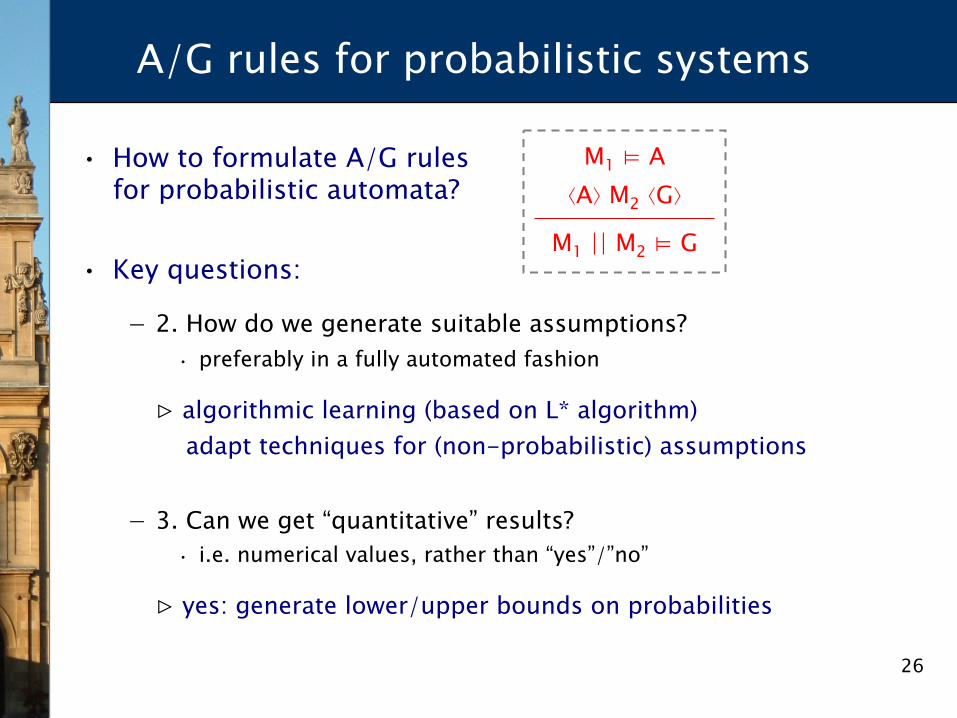
A/G rules for probabilistic systems
• How to formulate A/G rulesfor probabilistic automata?
• Key questions:
− 2. How do we generate suitable assumptions? • preferably in a fully automated fashion
▷ algorithmic learning (based on L* algorithm) adapt techniques for (non-probabilistic) assumptions
− 3. Can we get “quantitative” results? • i.e. numerical values, rather than “yes”/”no”
▷ yes: generate lower/upper bounds on probabilities
M1 ⊨ A
⟨A⟩ M2 ⟨G⟩
M1 || M2 ⊨ G
27
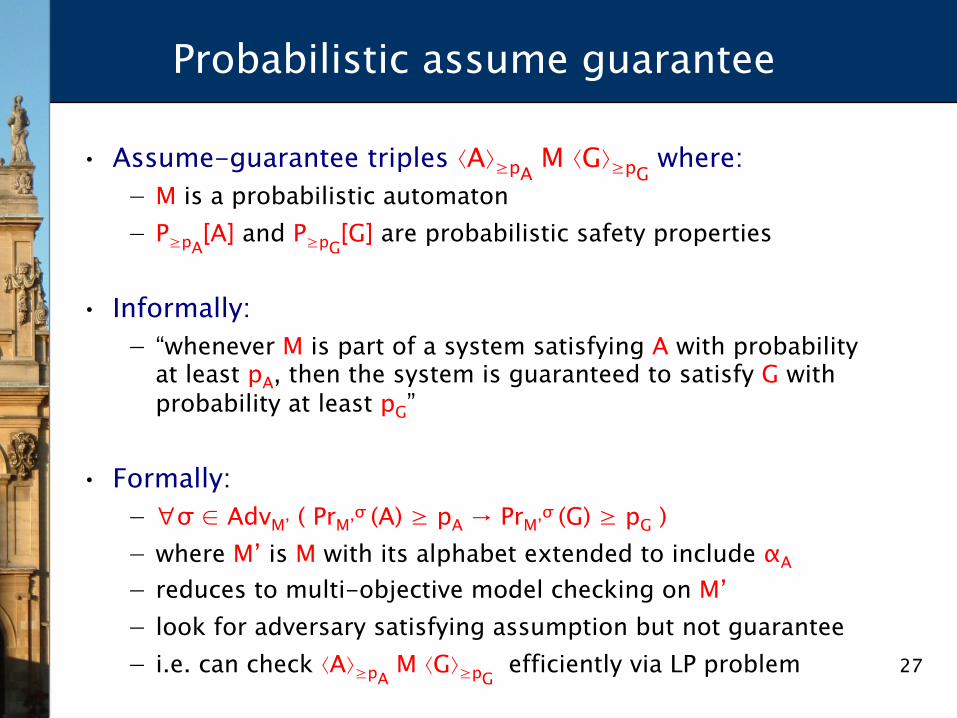
Probabilistic assume guarantee
• Assume-guarantee triples ⟨A⟩≥pA M ⟨G⟩≥pG
where: − M is a probabilistic automaton − P≥pA
[A] and P≥pG[G] are probabilistic safety properties
• Informally: − “whenever M is part of a system satisfying A with probability
at least pA, then the system is guaranteed to satisfy G with probability at least pG”
• Formally: − ∀σ ∈ AdvM’ ( PrM’
σ (A) ≥ pA → PrM’σ (G) ≥ pG )
− where M’ is M with its alphabet extended to include αA
− reduces to multi-objective model checking on M’ − look for adversary satisfying assumption but not guarantee − i.e. can check ⟨A⟩≥pA
M ⟨G⟩≥pG efficiently via LP problem
28
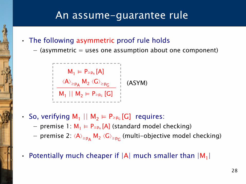
An assume-guarantee rule
• The following asymmetric proof rule holds − (asymmetric = uses one assumption about one component)
• So, verifying M1 || M2 ⊨ P≥pG [G] requires: − premise 1: M1 ⊨ P≥pA [A] (standard model checking) − premise 2: ⟨A⟩≥pA
M2 ⟨G⟩≥pG (multi-objective model checking)
• Potentially much cheaper if |A| much smaller than |M1|
M1 ⊨ P≥pA [A]
⟨A⟩≥pA M2 ⟨G⟩≥pG
M1 || M2 ⊨ P≥pG [G]
(ASYM)

29
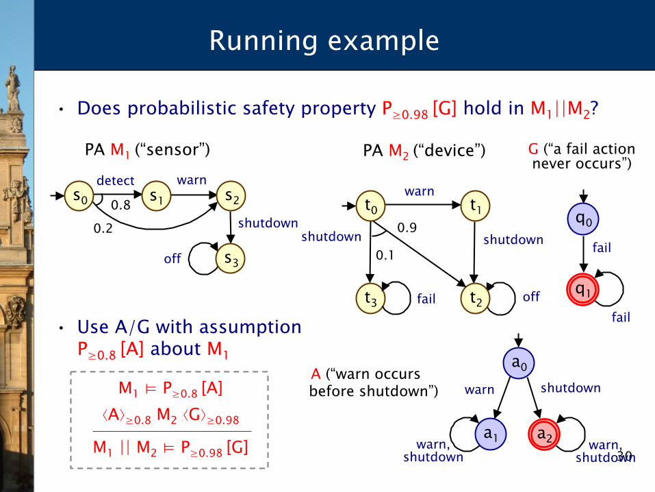
Running example
• Does probabilistic safety property P≥0.98 [G] hold in M1||M2?
PA M2 (“device”) PA M1 (“sensor”)
t1
0.1
warn
t2 t3
shutdown 0.9 shutdown
t0
fail off
s0
0.2
detect
s3
s1 0.8 shutdown
warn
off
s2
G (“a fail actionnever occurs”)
fail
fail
q0
q1
30
Running example
• Does probabilistic safety property P≥0.98 [G] hold in M1||M2?
• Use A/G with assumptionP≥0.8 [A] about M1
PA M2 (“device”) PA M1 (“sensor”)
t1
0.1
warn
t2 t3
shutdown 0.9 shutdown
t0
fail off
s0
0.2
detect
s3
s1 0.8 shutdown
warn
off
s2
G (“a fail actionnever occurs”)
fail
fail
q0
q1
A (“warn occursbefore shutdown”) shutdown warn
a0
a2 a1 warn, shutdown
warn, shutdown
M1 ⊨ P≥0.8 [A] ⟨A⟩≥0.8 M2 ⟨G⟩≥0.98
M1 || M2 ⊨ P≥0.98 [G]
31
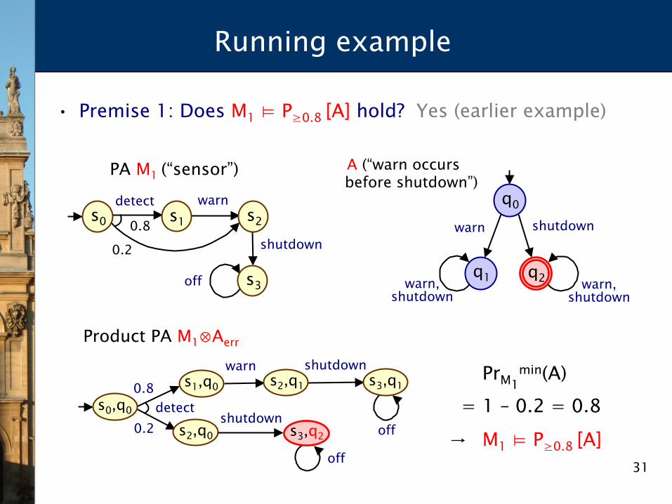
Running example
• Premise 1: Does M1 ⊨ P≥0.8 [A] hold? Yes (earlier example)
PA M1 (“sensor”) A (“warn occursbefore shutdown”)
shutdown warn
q0
q2 q1 warn, shutdown
warn, shutdown
s0,q0
0.2 detect
0.8
shutdown
warn s1,q0
s2,q0
s2,q1 s3,q1
shutdown
off
off
s3,q2
Product PA M1⊗Aerr
s0
0.2
detect
s3
s1 0.8 shutdown
warn
off
s2
PrM1min(A)
= 1 – 0.2 = 0.8 → M1 ⊨ P≥0.8 [A]
32
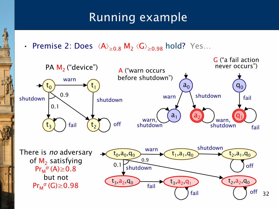
Running example
• Premise 2: Does ⟨A⟩≥0.8 M2 ⟨G⟩≥0.98 hold? Yes…
A (“warn occursbefore shutdown”)
shutdown warn
a0
a2 a1 warn, shutdown
warn, shutdown
G (“a fail actionnever occurs”)
fail
fail
q0
q1
PA M2 (“device”)
t1
0.1
warn
t2 t3
shutdown 0.9 shutdown
t0
fail off
t0,a0,q0 warn shutdown
t1,a1,q0
t3,a2,q0 fail t2,a2,q0
fail
t2,a1,q0
shutdown
off
off 0.9
0.1
t3,a2,q1
There is no adversary of M2 satisfying
PrMσ (A)≥0.8 but not
PrMσ (G)≥0.98

33
Running example
• Premise 2: Does ⟨A⟩≥0.8 M2 ⟨G⟩≥0.98 hold? Yes…
A (“warn occursbefore shutdown”)
shutdown warn
a0
a2 a1 warn, shutdown
warn, shutdown
G (“a fail actionnever occurs”)
fail
fail
q0
q1
PA M2 (“device”)
t1
0.1
warn
t2 t3
shutdown 0.9 shutdown
t0
fail off
t0,a0,q0 warn shutdown
t1,a1,q0
t3,a2,q0 fail t2,a2,q0
fail
t2,a1,q0
shutdown
off
off 0.9
0.1
t3,a2,q1
There is no adversary of M2⊗Aerr⊗Gerr satisfying
PrMσ (◊a2)≤0.2
and PrM
σ (◊q1)>0.02
34
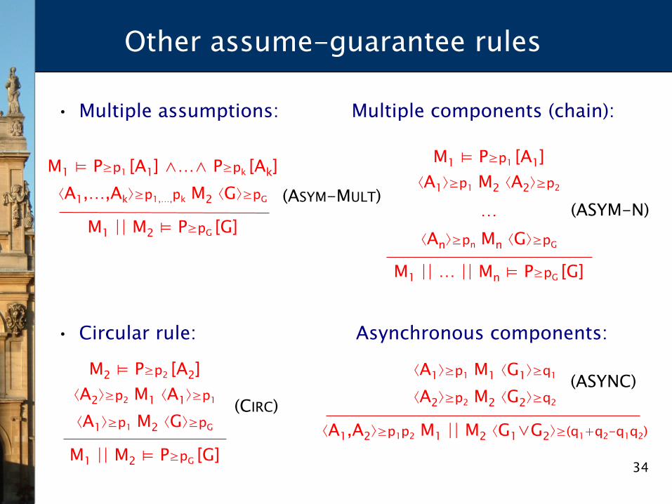
Other assume-guarantee rules
• Multiple assumptions: Multiple components (chain):
• Circular rule: Asynchronous components:
M1 ⊨ P≥p1 [A1] ∧…∧ P≥pk [Ak] ⟨A1,…,Ak⟩≥p1,…,pk M2 ⟨G⟩≥pG
M1 || M2 ⊨ P≥pG [G]
M2 ⊨ P≥p2 [A2] ⟨A2⟩≥p2 M1 ⟨A1⟩≥p1
⟨A1⟩≥p1 M2 ⟨G⟩≥pG
M1 || M2 ⊨ P≥pG [G]
M1 ⊨ P≥p1 [A1] ⟨A1⟩≥p1 M2 ⟨A2⟩≥p2
… ⟨An⟩≥pn Mn ⟨G⟩≥pG
M1 || … || Mn ⊨ P≥pG [G]
(ASYM-N)
(CIRC)
(ASYM-MULT)
⟨A1⟩≥p1 M1 ⟨G1⟩≥q1
⟨A2⟩≥p2 M2 ⟨G2⟩≥q2
⟨A1,A2⟩≥p1p2 M1 || M2 ⟨G1∨G2⟩≥(q1+q2-q1q2)
(ASYNC)
35
Implementation + Case studies
• Implemented using: − extension of PRISM model checker − added support for multi-objective model checking − built-in support for assume-guarantee in progress
• Two large case studies − randomised consensus algorithm (Aspnes & Herlihy)
• minimum probability consensus reached by round R − Zeroconf network protocol
• maximum probability network configures incorrectly • minimum probability network configured by time T
36
Experimental results
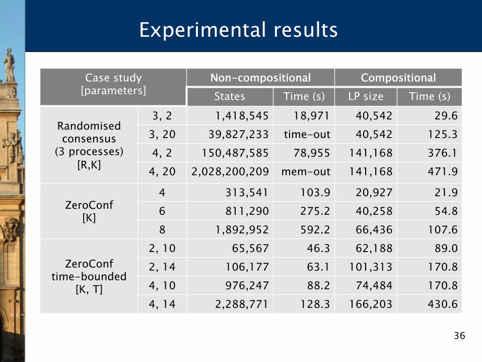
Case study [parameters]
Non-compositional Compositional States Time (s) LP size Time (s)
Randomised consensus
(3 processes) [R,K]
3, 2 1,418,545 18,971 40,542 29.6 3, 20 39,827,233 time-out 40,542 125.3 4, 2 150,487,585 78,955 141,168 376.1
4, 20 2,028,200,209 mem-out 141,168 471.9
ZeroConf [K]
4 313,541 103.9 20,927 21.9 6 811,290 275.2 40,258 54.8 8 1,892,952 592.2 66,436 107.6
ZeroConf time-bounded
[K, T]
2, 10 65,567 46.3 62,188 89.0 2, 14 106,177 63.1 101,313 170.8 4, 10 976,247 88.2 74,484 170.8 4, 14 2,288,771 128.3 166,203 430.6
37
Experimental results
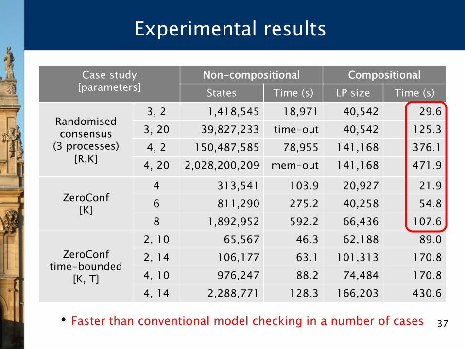
Case study [parameters]
Non-compositional Compositional States Time (s) LP size Time (s)
Randomised consensus
(3 processes) [R,K]
3, 2 1,418,545 18,971 40,542 29.6 3, 20 39,827,233 time-out 40,542 125.3 4, 2 150,487,585 78,955 141,168 376.1
4, 20 2,028,200,209 mem-out 141,168 471.9
ZeroConf [K]
4 313,541 103.9 20,927 21.9 6 811,290 275.2 40,258 54.8 8 1,892,952 592.2 66,436 107.6
ZeroConf time-bounded
[K, T]
2, 10 65,567 46.3 62,188 89.0 2, 14 106,177 63.1 101,313 170.8 4, 10 976,247 88.2 74,484 170.8 4, 14 2,288,771 128.3 166,203 430.6
• Faster than conventional model checking in a number of cases
38
Experimental results
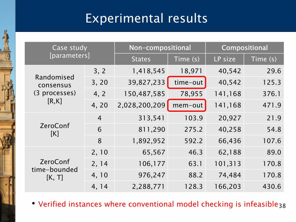
Case study [parameters]
Non-compositional Compositional States Time (s) LP size Time (s)
Randomised consensus
(3 processes) [R,K]
3, 2 1,418,545 18,971 40,542 29.6 3, 20 39,827,233 time-out 40,542 125.3 4, 2 150,487,585 78,955 141,168 376.1
4, 20 2,028,200,209 mem-out 141,168 471.9
ZeroConf [K]
4 313,541 103.9 20,927 21.9 6 811,290 275.2 40,258 54.8 8 1,892,952 592.2 66,436 107.6
ZeroConf time-bounded
[K, T]
2, 10 65,567 46.3 62,188 89.0 2, 14 106,177 63.1 101,313 170.8 4, 10 976,247 88.2 74,484 170.8 4, 14 2,288,771 128.3 166,203 430.6
• Verified instances where conventional model checking is infeasible
39
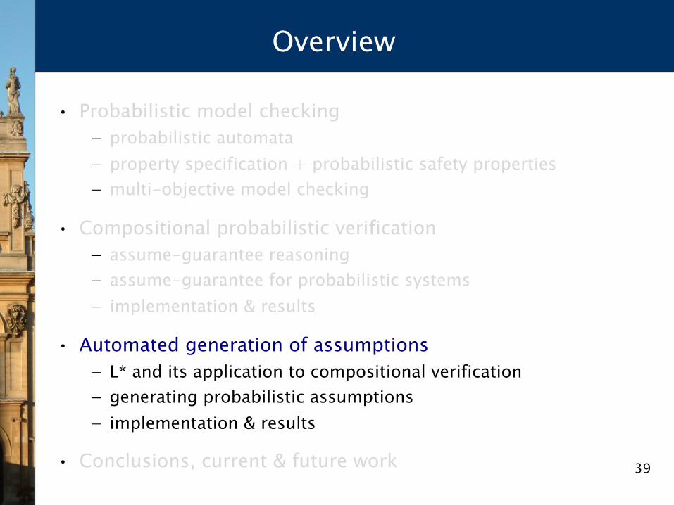
Overview
• Probabilistic model checking − probabilistic automata − property specification + probabilistic safety properties − multi-objective model checking
• Compositional probabilistic verification − assume-guarantee reasoning − assume-guarantee for probabilistic systems − implementation & results
• Automated generation of assumptions − L* and its application to compositional verification − generating probabilistic assumptions − implementation & results
• Conclusions, current & future work
40
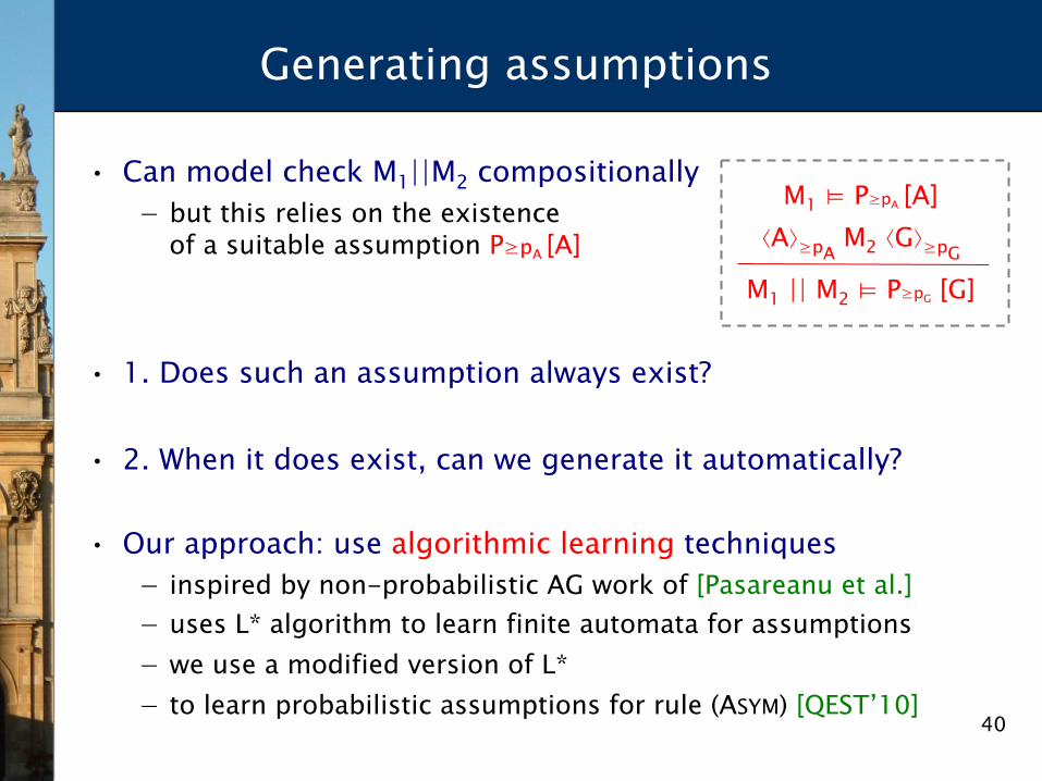
Generating assumptions
• Can model check M1||M2 compositionally − but this relies on the existence
of a suitable assumption P≥pA [A]
• 1. Does such an assumption always exist?
• 2. When it does exist, can we generate it automatically?
• Our approach: use algorithmic learning techniques − inspired by non-probabilistic AG work of [Pasareanu et al.] − uses L* algorithm to learn finite automata for assumptions − we use a modified version of L* − to learn probabilistic assumptions for rule (ASYM) [QEST’10]
M1 ⊨ P≥pA [A]
⟨A⟩≥pA M2 ⟨G⟩≥pG
M1 || M2 ⊨ P≥pG [G]
41
The L* learning algorithm
• The L* algorithm [Angluin] − learns an unknown regular language L, as a (minimal) DFA
• Based on “active” learning − relies on existence of a “teacher” to guide the learning − answers two type of queries: “membership” and “equivalence” − membership: “is trace (word) t in the target language L?”
• stores results of membership queries in observation table • based on these, generates conjectures A for the automata
− equivalence: “does automata A accept the target language L”? • if not, teacher must return counterexample c • (c is a word in the symmetric difference of L and L(A))
42
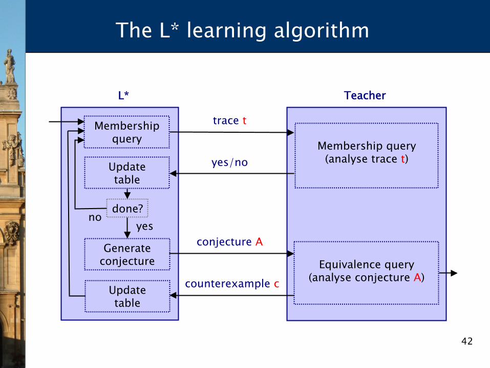
The L* learning algorithm
Update table
Generate conjecture
Membership query
Update table
Membership query (analyse trace t)
Equivalence query (analyse conjecture A)
trace t
counterexample c
conjecture A
yes/no
done? yes
Teacher L*
no
43
L* for assume-guarantee
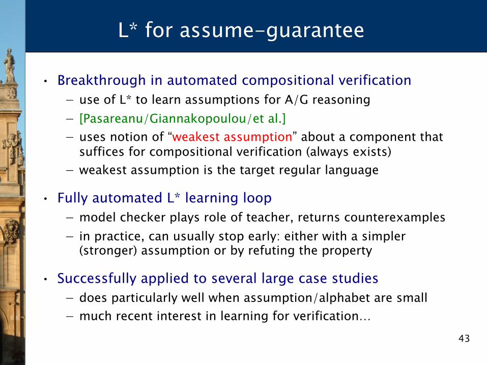
• Breakthrough in automated compositional verification − use of L* to learn assumptions for A/G reasoning − [Pasareanu/Giannakopoulou/et al.] − uses notion of “weakest assumption” about a component that
suffices for compositional verification (always exists) − weakest assumption is the target regular language
• Fully automated L* learning loop − model checker plays role of teacher, returns counterexamples − in practice, can usually stop early: either with a simpler
(stronger) assumption or by refuting the property
• Successfully applied to several large case studies − does particularly well when assumption/alphabet are small − much recent interest in learning for verification…
44
Probabilistic assumption generation
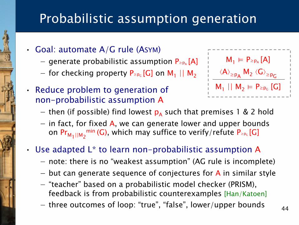
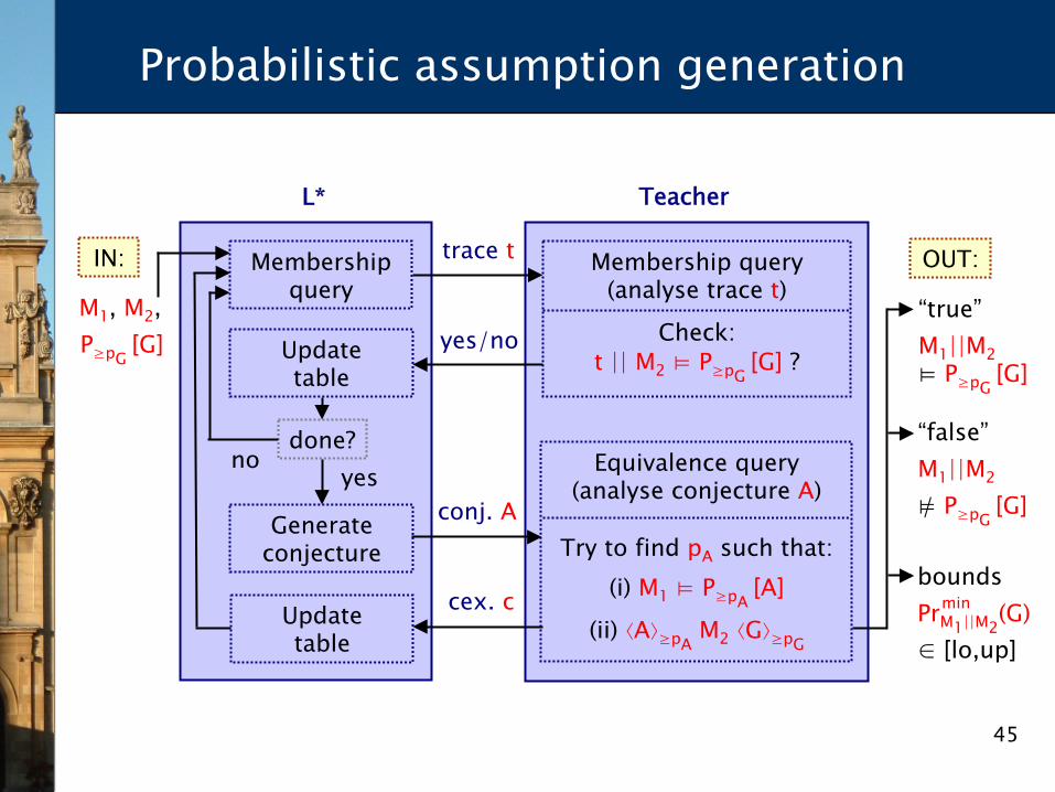
• Goal: automate A/G rule (ASYM) − generate probabilistic assumption P≥pA [A] − for checking property P≥pG [G] on M1 || M2
• Reduce problem to generation ofnon-probabilistic assumption A − then (if possible) find lowest pA such that premises 1 & 2 hold − in fact, for fixed A, we can generate lower and upper bounds
on PrM1||M2min (G), which may suffice to verify/refute P≥pG [G]
• Use adapted L* to learn non-probabilistic assumption A − note: there is no “weakest assumption” (AG rule is incomplete) − but can generate sequence of conjectures for A in similar style − “teacher” based on a probabilistic model checker (PRISM),
feedback is from probabilistic counterexamples [Han/Katoen] − three outcomes of loop: “true”, “false”, lower/upper bounds
M1 ⊨ P≥pA [A]
⟨A⟩≥pA M2 ⟨G⟩≥pG
M1 || M2 ⊨ P≥pG [G]
45
Probabilistic assumption generation
Update table
Generate conjecture
Membership query
Update table
Membership query (analyse trace t)
Check: t || M2 ⊨ P≥pG [G] ?
Equivalence query (analyse conjecture A)
Try to find pA such that: (i) M1 ⊨ P≥pA [A]
(ii) ⟨A⟩≥pA M2 ⟨G⟩≥pG
trace t
cex. c
conj. A
yes/no
done? yes
“true” M1||M2 ⊨ P≥pG [G]
“false” M1||M2 ⊨ P≥pG [G] /
M1, M2, P≥pG [G]
Teacher L*
OUT:
bounds PrM1||M2
(G) ∈ [lo,up]
IN:
no
min
46
Implementation + Case studies
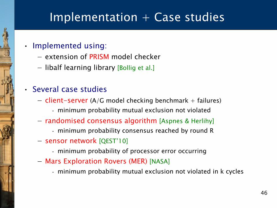
• Implemented using: − extension of PRISM model checker − libalf learning library [Bollig et al.]
• Several case studies − client-server (A/G model checking benchmark + failures)
• minimum probability mutual exclusion not violated − randomised consensus algorithm [Aspnes & Herlihy]
• minimum probability consensus reached by round R − sensor network [QEST’10]
• minimum probability of processor error occurring − Mars Exploration Rovers (MER) [NASA]
• minimum probability mutual exclusion not violated in k cycles
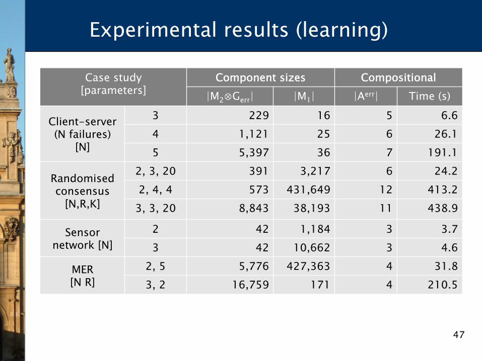
47
Experimental results (learning)
Case study [parameters]
Component sizes Compositional |M2⊗Gerr| |M1| |Aerr| Time (s)
Client-server (N failures)
[N]
3 229 16 5 6.6 4 1,121 25 6 26.1 5 5,397 36 7 191.1
Randomised consensus
[N,R,K]
2, 3, 20 391 3,217 6 24.2 2, 4, 4 573 431,649 12 413.2
3, 3, 20 8,843 38,193 11 438.9
Sensor network [N]
2 42 1,184 3 3.7 3 42 10,662 3 4.6
MER [N R]
2, 5 5,776 427,363 4 31.8 3, 2 16,759 171 4 210.5
48
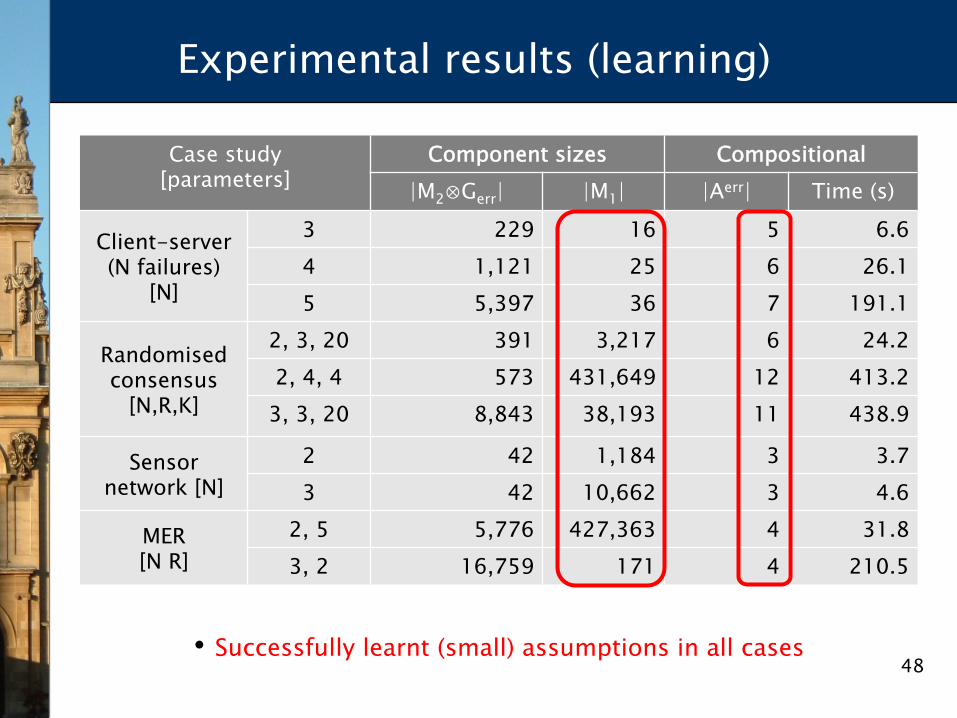
Experimental results (learning)
Case study [parameters]
Component sizes Compositional |M2⊗Gerr| |M1| |Aerr| Time (s)
Client-server (N failures)
[N]
3 229 16 5 6.6 4 1,121 25 6 26.1 5 5,397 36 7 191.1
Randomised consensus
[N,R,K]
2, 3, 20 391 3,217 6 24.2 2, 4, 4 573 431,649 12 413.2
3, 3, 20 8,843 38,193 11 438.9
Sensor network [N]
2 42 1,184 3 3.7 3 42 10,662 3 4.6
MER [N R]
2, 5 5,776 427,363 4 31.8 3, 2 16,759 171 4 210.5
• Successfully learnt (small) assumptions in all cases
49
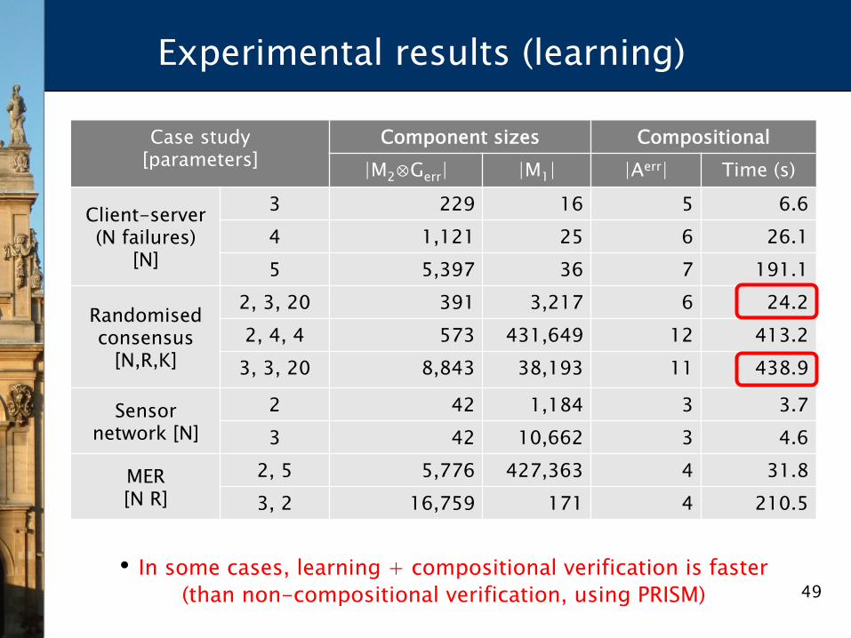
Experimental results (learning)
Case study [parameters]
Component sizes Compositional |M2⊗Gerr| |M1| |Aerr| Time (s)
Client-server (N failures)
[N]
3 229 16 5 6.6 4 1,121 25 6 26.1 5 5,397 36 7 191.1
Randomised consensus
[N,R,K]
2, 3, 20 391 3,217 6 24.2 2, 4, 4 573 431,649 12 413.2
3, 3, 20 8,843 38,193 11 438.9
Sensor network [N]
2 42 1,184 3 3.7 3 42 10,662 3 4.6
MER [N R]
2, 5 5,776 427,363 4 31.8 3, 2 16,759 171 4 210.5
• In some cases, learning + compositional verification is faster (than non-compositional verification, using PRISM)
50
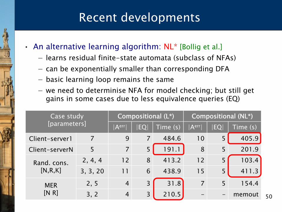
Recent developments
• An alternative learning algorithm: NL* [Bollig et al.] − learns residual finite-state automata (subclass of NFAs) − can be exponentially smaller than corresponding DFA − basic learning loop remains the same − we need to determinise NFA for model checking; but still get
gains in some cases due to less equivalence queries (EQ)
Case study [parameters]
Compositional (L*) Compositional (NL*) |Aerr| |EQ| Time (s) |Aerr| |EQ| Time (s)
Client-server1 7 9 7 484.6 10 5 405.9 Client-serverN 5 7 5 191.1 8 5 201.9
Rand. cons. [N,R,K]
2, 4, 4 12 8 413.2 12 5 103.4 3, 3, 20 11 6 438.9 15 5 411.3
MER [N R]
2, 5 4 3 31.8 7 5 154.4 3, 2 4 3 210.5 - - memout
51
Recent developments…
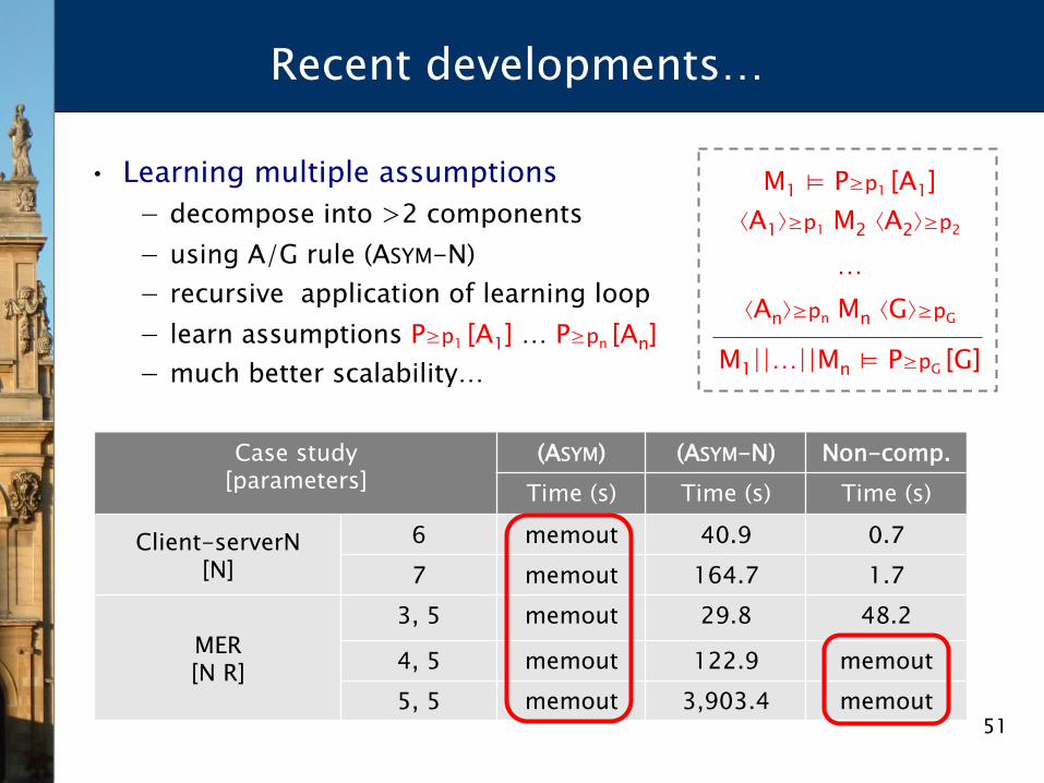
• Learning multiple assumptions − decompose into >2 components − using A/G rule (ASYM-N) − recursive application of learning loop − learn assumptions P≥p1 [A1] … P≥pn [An] − much better scalability…
M1 ⊨ P≥p1 [A1] ⟨A1⟩≥p1 M2 ⟨A2⟩≥p2
… ⟨An⟩≥pn Mn ⟨G⟩≥pG
M1||…||Mn ⊨ P≥pG [G]
Case study [parameters]
(ASYM) (ASYM-N) Non-comp. Time (s) Time (s) Time (s)
Client-serverN [N]
6 memout 40.9 0.7 7 memout 164.7 1.7
MER [N R]
3, 5 memout 29.8 48.2
4, 5 memout 122.9 memout 5, 5 memout 3,903.4 memout
52
Conclusions
• Probabilistic model checking − active research area, efficient tools, widely used − but scalability is still the biggest challenge
• Compositional probabilistic verification − assume-guarantee framework for probabilistic automata − reduction to (efficient) multi-objective model checking − verified safety/performance on several large case studies − cases where infeasible using non-compositional verification − full automation: learning-based generation of assumptions
• But this is only the beginning…