Solar Phys (2017) 292:69DOI 10.1007/s11207-017-1090-7

Probabilistic Solar Wind and Geomagnetic ForecastingUsing an Analogue Ensemble or “Similar Day” Approach

M.J. Owens1 · P. Riley2 · T.S. Horbury3

Received: 16 December 2016 / Accepted: 30 March 2017 / Published online: 19 April 2017© The Author(s) 2017. This article is published with open access at Springerlink.com

Abstract Effective space-weather prediction and mitigation requires accurate forecastingof near-Earth solar-wind conditions. Numerical magnetohydrodynamic models of the solarwind, driven by remote solar observations, are gaining skill at forecasting the large-scalesolar-wind features that give rise to near-Earth variations over days and weeks. There re-mains a need for accurate short-term (hours to days) solar-wind forecasts, however. In thisstudy we investigate the analogue ensemble (AnEn), or “similar day”, approach that wasdeveloped for atmospheric weather forecasting. The central premise of the AnEn is thatpast variations that are analogous or similar to current conditions can be used to provide agood estimate of future variations. By considering an ensemble of past analogues, the AnEnforecast is inherently probabilistic and provides a measure of the forecast uncertainty. Weshow that forecasts of solar-wind speed can be improved by considering both speed anddensity when determining past analogues, whereas forecasts of the out-of-ecliptic magneticfield [BN] are improved by also considering the in-ecliptic magnetic-field components. Ingeneral, the best forecasts are found by considering only the previous 6 – 12 hours of ob-servations. Using these parameters, the AnEn provides a valuable probabilistic forecast forsolar-wind speed, density, and in-ecliptic magnetic field over lead times from a few hoursto around four days. For BN, which is central to space-weather disturbance, the AnEn onlyprovides a valuable forecast out to around six to seven hours. As the inherent predictabilityof this parameter is low, this is still likely a marked improvement over other forecast meth-ods. We also investigate the use of the AnEn in forecasting geomagnetic indices Dst and Kp.The AnEn provides a valuable probabilistic forecast of both indices out to around four days.We outline a number of future improvements to AnEn forecasts of near-Earth solar-windand geomagnetic conditions.

Keywords Solar wind · Space weather · Heliospheric magnetic field

B M.J. Owensm.j.owens@reading.ac.uk

1 Space and Atmospheric Electricity Group, Department of Meteorology, University of Reading,Earley Gate, PO Box 243, Reading RG6 6BB, UK

2 Predictive Science Inc., 9990 Mesa Rim Rd, Suite 170, San Diego, CA 92121, USA

3 Blackett Laboratory, Imperial College London, London SW7 2BZ, UK

69 Page 2 of 16 M.J. Owens et al.

1. Introduction

The purpose of space-weather forecasting is, ultimately, to improve decision-making capa-bility for a range of end users, including (but not limited to) power companies, satellite op-erators, the aviation industry, communication companies, and human-spaceflight controllers(Hapgood, 2011; Cannon et al., 2013). While accuracy is central to any useful forecast, dif-ferent aspects of the forecast, e.g. ratio of false alarms to missed events, reliability of “allclear” forecasts, forecast lead time, correct event occurrence statistics, and ability to predictextremes, will be more or less important for different operational applications.

Physics-based, long lead-time (i.e. greater than approximately 40 minutes, the nominalL1-to-Earth solar-wind propagation time) space-weather forecasting requires prediction ofnear-Earth solar-wind conditions on the basis of remote solar or heliospheric observations.This is typically provided by deterministic numerical magnetohydrodynamic (MHD) mod-els (e.g. Riley, Linker, and Mikic, 2001; Odstrcil et al., 2004; Tóth et al., 2005). Ensemblesof numerical solar-wind MHD models, using multiple runs of the numerical model withstochastic perturbations to the initial conditions (e.g. Cash et al., 2015), are beginning to beused operationally, although the number of ensemble members is limited by computationalpower, and the range of perturbations is poorly constrained by observations. More funda-mentally, it is not clear that the probability density function (PDF) generated from the spreadin ensemble members accurately represents the uncertainty in the forecast. In particular, ifthe model has any systematic bias, such as an under-prediction of the heliospheric-magnetic-field (HMF) intensity [B], then the ensemble PDF of B will also be skewed to low valuesand not represent the true likelihood of a given value of B .

Similar issues are faced by terrestrial atmospheric-weather forecasting. Before the adventof numerical weather prediction (NWP) models, and especially the forecast skill advancethat came with the advent of ensemble NWP (e.g. Leutbecher and Palmer, 2008 and refer-ences therein), “similar day” or analogue forecasting (AF) methods were widely used. Thebasic premise is that if close matches (or analogues) to the current atmospheric conditionscan be identified in historical observations, these analogues will provide a good estimateof conditions in the future (e.g. van den Dool, 1989 and references therein). By consider-ing an “ensemble” of past analogues, a probabilistic forecast for future conditions can beconstructed. As this is the result of observations, it is inherently bias-free. AF is actuallyof limited use for terrestrial weather forecasting as the atmospheric system is inherentlychaotic, and so it is a poor assumption that two atmospheric states that are initially closewill remain so in the future (Lorenz, 1969). For solar-wind forecasting, which is far moreof a system “driven” by boundary conditions, the prospects are more promising, as we shalldemonstrate.

AF has since found a new role within atmospheric forecasting (Delle Monache et al.,2013). Historical NWP forecasts are analysed for times analogous to the current forecaststate. These times are used to produce an ensemble of the observed conditions. This servestwo purposes: Firstly, it corrects for any bias in the NWP forecast. Secondly, with little ad-ditional computational cost or need to specify initial condition perturbations, it transformsa single deterministic forecast into probabilistic forecast with an accurate bias-free assess-ment of the uncertainty in the forecast. This approach will undoubtedly be useful for solar-wind forecasting, once a long enough (e.g. decades) catalogue of historical MHD solar-windforecasts has been amassed. At present, we investigate the use of a purely observation-basedanalogue ensemble (AnEn) for statistical solar-wind forecasting, rather than in conjunctionwith a model.

The concept of analogue or “similar day” forecasting has previously been investigatedfor specific space-weather uses, with pattern matching within discrete solar-wind events,

Analogue Ensemble Solar Wind Forecasting Page 3 of 16 69

specifically magnetic clouds (Chen, Cargill, and Palmadesso, 1997) and high-speed streams(Bussy-Virat and Ridley, 2016). More recently, Riley et al. (2017) have demonstrated thepotential of analogue forecasts through simple pattern matching for various solar-wind con-ditions. Considering solar-wind parameters independently, and fixing the number of ana-logue periods at 50 and the period over which they are determined at 24 hours, they showedsignificant forecast skill for a few days lead time in solar-wind speed, density, and temper-ature, but only a few hours for the out-of-ecliptic magnetic-field component. Nonlinear ap-proaches, particularly neural networks, which implicitly involve analogue-forecasting ideas,have been widely used for predicting Kp, one of the most widely used indices of geomag-netic disturbance (Detman and Joselyn, 1999; Boberg, Wintoft, and Lundstedt, 2000; Winget al., 2005). These are typically used to assess the recent solar-wind conditions and give Kpforecasts with a lead time of about three hours (e.g. Solares et al., 2016). While not directlyan analogue forecast as such, explicit decomposition of sunspot, irradiance, and geomag-netic time series into the frequency domain has also been shown to have predictive powerover short (e.g. one- to seven-day) forecast lead times (Reikard, 2016).

In this study, we build on the results of Riley et al. (2017) to investigate the purelyAnEn approach for continuous probabilistic solar-wind and geomagnetic forecasting. Weperform a sensitivity analysis of the AnEn forecast skill to the choice of the time periodand parameters over which the analogy is computed, as well as the number of analogousperiods used to produce the ensemble. We then quantify the potential economic value of theprobabilistic AnEn forecasts relative to persistence and climatology.

2. Producing an Ensemble Analogue (AnEn) for the Solar Wind

To produce a solar-wind AnEn forecast, we use the OMNI series of near-Earth in-situ space-craft observations (King and Papitashvili, 2005) at one-hour resolution. The inclination an-gle of the Ecliptic plane to the solar-rotation direction means that there are entirely geometrictrends in the magnetic-field and solar-wind flow vectors. In geocentric-solar-ecliptic (GSE)coordinates, predictability is thus present in the y- and z-components of the solar-wind flowand magnetic-field time series that is unrelated to solar-wind structures or variability, butresults purely from the variation in the GSE coordinate system over the Earth’s orbit (e.g.Rosenberg and Coleman, 1969; Russell and McPherron, 1973). In this study, data are con-sidered in the heliographic radial-tangential-normal (RTN) coordinate system, where thenormal is along the solar-rotation axis and the tangential is to the solar-rotation direction.The RTN coordinate system removes the orbital or geometric trends effects in the near-Earthsolar-wind parameters and enables the predictability of solar-wind structures to be studiedin isolation. For space-weather forecasting purposes, the radial solar-wind flow speed [VR]and the component of the HMF normal to the solar-rotation plane [BN] are the critical pa-rameters, as they are the primary contributors to the dawn-to-dusk electric field that controlsreconnection with the magnetospheric field (Dungey, 1961). Owing to the inclination of theEarth’s magnetosphere and orbital plane to the solar-rotation plane, the HMF componentalong the solar-rotation direction [BT] also leads to a magnetic field anti-parallel to the noseof the magnetosphere, in a manner that varies systematically with both day of year and timeof day (Lockwood et al., 2016). The solar-wind density [NP] also affects the compressionof the magnetosphere and hence the efficiency of the magnetic coupling between the he-liospheric and magnetospheric magnetic fields. These are the four solar-wind parametersinvestigated in this study.

69 Page 4 of 16 M.J. Owens et al.

Using OMNI data in RTN coordinates, the AnEn methodology is first demonstrated forthe simplest case: forecasting a single solar-wind parameter [P ] in near-Earth space from thecurrent time [t0] out to a forecast lead-time [t0 + TF], where TF is the length of the forecastwindow. The similarity of recent solar-wind conditions to historic observations is quantifiedusing the mean-square error (MSE) between P during the training window, t0 − TT to t0(where TT is the length of the training window), and P at all previously observed intervals,i.e. tn − TT to tn, for all values of tn between the start of OMNI data and t0. Obviously, fortrue forecasting purposes, only training intervals before t0 will be available. For solar-windAnEn development, however, the database can be enlarged by using intervals both beforeand after t0, although the forecast window itself is obviously excluded. The analogues are theNEN periods with the lowest MSE values. The forecast is then assembled from the ensembleof the NEN time series over the period tn to tn + TF.

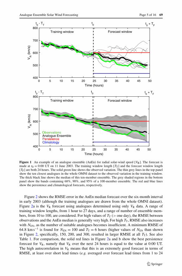
An example is shown in Figure 1 for the radial solar-wind speed [VR] variation on 11June 2003. The training and forecast window lengths, TT and TF, are both 24 hours. Thegreen line shows the observed variation, which shows a fairly steady decline in both thetraining and forecast windows. The thin grey lines in the top panel show the ten closestanalogues in the training window, drawn from the entire OMNI dataset. There is a greatdeal of spread in this ten-member ensemble during the forecast window, but the median,shown as the thick black line, does show a downward variation, as observed. This variationwould not be obtained by assuming, e.g. persistence (shown in red) of the last observedvalue (approximately 600 km s−1) over the forecast window. Similarly, assuming the cli-matological value of VR, taken to be the mean over the whole OMNI dataset (433 km s−1,shown in blue), would provide a poor forecast. The bottom panel shows the same analysisfor NEN = 100, with the grey shaded bands containing 67%, 90%, and 95% of the ensemblemembers. Such assessments of uncertainty are fully nonparametric and do not assume thatthe data are normally distributed.

Note that the top panel of Figure 1 shows a number of discontinuous lines, which are theresult of data gaps in the forecast windows of individual analogues. As the forecast medianand confidence intervals are calculated independently at each time step, data gaps are simplyexcluded. This means that when a large number of analogues contain data gaps at a givenforecast time, the reliability of the median reduces and the width of the confidence intervalsexpands. We limit this effect by requiring at least 75% data coverage in both the trainingand forecast windows.

The quality of the forecast obtained in this manner depends critically on a number of pa-rameters, particularly TT, NEN, and the choice of training parameter(s). In the initial study ofRiley et al. (2017), TT was fixed at 24 hours, NEN was fixed at 50, and the closest analogueswere determined only using the parameter being forecast. In order to assess the optimumvalues for solar-wind forecasting, we test a range of values and parameters for the period1 January 2003 to 31 June 2003. While there is nothing particularly special about this pe-riod, it does contain some prolonged periods of fast and slow wind, as well as a numberof interplanetary coronal mass ejections, testing the AnEn over a wide range of conditions.A longer interval is not used for computational reasons. It is not possible to fully explorethe parameter space in a systematic fashion for the same reason. Instead, we explore eachvariable in turn and consider only the root-mean square error (RMSE) between observationsand ensemble median. Note that by considering only the ensemble median, this method doesnot fully exploit the power of a probabilistic forecast, discussed further below. At 0:00 UTfor each day in the six-month period, we compute the AnEn median forecast over the next24 hours and compare that with observations (the analogue periods, however, can begin atany UT). Thus the RMSE is computed for a range of forecast lead times from 1 to 24 hours.Performance at each lead time is considered below.

Analogue Ensemble Solar Wind Forecasting Page 5 of 16 69

Figure 1 An example of an analogue ensemble (AnEn) for radial solar-wind speed [VR]. The forecast ismade at t0 = 0:00 UT on 11 June 2003. The training window length [TT] and the forecast window length[TF] are both 24 hours. The solid green line shows the observed variation. The thin grey lines in the top panelshow the ten closest analogues in the whole OMNI dataset to the observed variation in the training window.The thick black line shows the median of this ten-member ensemble. The grey shaded regions in the bottompanel show the bands containing 68%, 90%, and 95% of a 100-member ensemble. The red and blue linesshow the persistence and climatological forecasts, respectively.

Figure 2 shows the RMSE error in the AnEn median forecast over the six-month intervalin early 2003 (although the training analogues are drawn from the whole OMNI dataset).Figure 2a is the VR forecast using analogues determined using only VR data. A range oftraining window lengths, from 1 hour to 27 days, and a range of number of ensemble mem-bers, from 10 to 100, are considered. For high values of TT (> one day), the RMSE betweenobservations and the AnEn median is generally very high. For high TT, RMSE also increaseswith NEN, as the number of suitable analogues becomes insufficient. A minimum RMSE of64.8 km s−1 is found for NEN = 100 and TT = 6 hours (higher values of NEN than shownin Figure 2, specifically, 150, 200, and 300, resulted in larger RMSE at all TT). See alsoTable 1. For comparison, the solid red lines in Figure 2a and b show the best persistenceforecast for VR, namely that VR over the next 24 hours is equal to the value at 0:00 UT.The high autocorrelation in VR means that this is an extremely good forecast in terms ofRMSE, at least over short lead times (e.g. averaged over forecast lead times from 1 to 24

69 Page 6 of 16 M.J. Owens et al.

Figure 2 The RMSE between observations and the AnEn median over the period 1 January 2003 to 1 July2003 for a range of training window lengths and number of ensemble members. Panels a and b show theRMSE in the median VR forecast using analogues determined from (a) VR only and (b) VR and NP. Solid,dashed, dot–dashed, and dotted lines show NEN = 100, 75, 50, and 10, respectively. The solid red lines showthe best persistence forecast. Panels c and d show the RMSE in the BN forecast using analogues determinedfrom (c) BN only and (d) BN and BT. The solid blue lines show the climatological forecast.

hours, it outperforms all current numerical solar-wind models (Owens et al., 2008), as wellas 27-day persistence (Owens et al., 2013)), although that does not necessarily make it auseful forecast for operational decision making. For this six-month test period, persistenceresults in an RMSE of 63.2 km s−1, lower than any of the AnEn forecasts considered in Fig-ure 2a. The “best” AnEn parameters result in an RMSE of 64.8 km s−1, this suggest that atbest the AnEn approaches persistence. Conversely, a climatological forecast of VR (i.e. thatVR = 433 km s−1 at all times) is very poor, resulting in an RMSE of 190 km s−1 (hence it isnot shown in the figure).

Analogue Ensemble Solar Wind Forecasting Page 7 of 16 69

Table 1 Summary of the training parameters that give the lowest RMSE over the interval 1 January 2003 – 1July 2003 for the AnEn median of various forecast parameters.

Forecastparameter

Best trainingparameter(s)

Best NEN Best[hours]

TT AnEnmedian

RMSE

Persistence Climatology

BT BT 100 6 3.42 nT 4.19 nT 4.50 nT

BN BT, BN 100 6 2.92 nT 4.24 nT 2.94 nT

VR VR, NP 100 6 61.6 km s−1 63.2 km s−1 190 km s−1

NP VR, NP 100 12 2.79 cm−3 4.22 cm−3 3.49 cm−3

Of course, there is no reason why the analogue periods have to be selected solely on thebasis of the forecast parameter (as in the VR forecast discussed above). Figure 2b shows theRMSE in the AnEn median VR forecast using analogue periods determined by both VR andNP in the training window. In order to combine RMSE in different solar-wind parametersmeasured in different physical units, it is necessary to first convert them into a normalisedquantity. To achieve this, the cumulative distribution functions (CDFs) of VR and NP arecomputed over the whole OMNI dataset. The time series of VR and NP are then convertedinto rank within their respective CDFs. RMSE in the training window is then calculated onthe basis of CDF rank. The VR and NP rank RMSEs are then multiplied together and theanalogues are taken to be the periods with the lowest values.

Figure 2b shows that for NEN > 10, the AnEn median forecast of VR using analoguesdetermined by both VR and NP performs better than persistence at TT = 6 hours. The lowestRMSE is for NEN = 100 and TT = 6 hours, resulting in an RMSE of 61.6 km s−1. For theAnEn forecast of NP (not shown), there is a similar situation: over the period January – June2003, a persistence forecast of NP gives an RMSE of 4.22 cm−3. A climatological forecastof NP = 6.74 cm−3 gives an RMSE of 3.49 cm−3. The best AnEn median forecast for NP

trained on just NP is TT = 12 hours and NEN = 100, giving an RMSE of 2.88 cm−3. Trainingthe AnEn on both VR and NP, however, gives an RMSE = 2.79 cm−3 for TT = 12 hours andNEN = 100.

Figure 2c shows the RMSE in BN using analogues determined by BN. The dashed lineshows the climatological forecast, i.e. BN = 0, which results in an RMSE of 2.94 nT, betterthan the current numerical and 27-day persistence forecasts, although it is likely to be of littlevalue as a forecast for operators. (The lack of autocorrelation in the BN time series meansthat the 1- to 24-hour persistence forecasts of BN are poor, giving an RMSE of 4.09 nT.Hence it is not shown in the figure.) For increasing NEN and TT, the AnEn forecast tendstowards climatology. For large NEN (i.e. >75), the AnEn forecast using TT between 3 and12 hours has an RMSE that is just lower than persistence. Figure 2d shows the same results,but for analogues determined on the basis of both BN and BT. For NEN > 50 and TT around6 hours, the median AnEn forecast is improved slightly.

The optimum AnEn parameters and the resulting RMSE are summarised in Table 1. Ob-viously, it is also necessary to quantify whether the differences in RMSE between the variousforecast types actually lead to a meaningful increase in an operator’s ability to successfullytake action. The utility of a forecast depends greatly on the particular application. Thus inthe probabilistic AnEn section, we also compute the “potential economic value” over a rangeof operational scenarios.

69 Page 8 of 16 M.J. Owens et al.

Figure 3 Average forecast RMSE over 1996 – 2015 as a function of forecast lead time for (a) VR, (b) NP,(c) BN, and (d) BT. Black, red, and blue lines show the AnEn, persistence, and climatological forecasts,respectively.

3. Performance of the Deterministic Solar-Wind AnEn over 1996 – 2014

We now investigate the performance of the AnEn using the parameters in Table 1 over amuch longer period, covering 1 January 1996 to 1 January 2015. This 19-year interval almostspans the period of near-complete OMNI data coverage. No attempt is made to remove orisolate the interplanetary manifestations of coronal mass ejections, which are treated in theexact same manner as any other solar-wind interval. Forecasts (be it AnEn, persistence, orclimatological) are made at 0:00 UT for every day in this interval and the average RMSEcomputed for a range of lead times, from 1 hour to 30 days.

Figure 3 shows the average RMSE as a function of forecast lead time. Panels a, b, c,and d show forecasts of VR, NP, BN, and BT, respectively. The climatological forecasts(blue) assume that the mean values of the forecast parameters, computed over the entireOMNI dataset, persist at all times. Thus the average RMSE for climatology is approximatelyconstant over all lead times, with a value of around 80 km s−1 for VR, 3.5 cm−3 for NP, 1.9 nTfor BN, and 3 nT for BT. The persistence forecasts, in red, assume that the hourly values ofthe forecast parameters at 0:00 UT persist over the forecast window. For all parameters, theaverage RMSE for persistence is small initially (as the current value of, e.g., VR is closelycorrelated with the value one hour previously), but grows rapidly with increased forecastlead time. For VR, NP, and BT, persistence out-performs climatology for forecast lead timesup to 15 – 30 hours. For BN, however, the RMSE for persistence is higher than climatologyeven at a lead time of two hours, demonstrating the short autocorrelation time in the BN timeseries and the inherent difficulty in BN prediction (e.g. Lockwood et al., 2016 and referencestherein).

Analogue Ensemble Solar Wind Forecasting Page 9 of 16 69

The AnEn forecasts, in black, use the parameters outlined in Table 1. The RMSE iscomputed between the AnEn median and observed time series. For VR and NP, persistenceoutperforms (i.e. provides a forecast with lower RMSE) the AnEn median for very shortlead times, <5 and <3 hours, respectively. For longer lead times, the AnEn median isbetter than both persistence and climatology. The RMSE in the AnEn grows with increasingforecast lead time, but at a much slower rate than persistence. As for persistence, the AnEnRMSE plateaus at a forecast lead-time of around 100 hours, but the AnEn reaches a valuelower than the climatological RMSE. This is due to the climatology being calculated overthe whole OMNI dataset, which results in a different mean value than over the 1996 – 2015test period, primarily as a result of solar-cycle sampling. The AnEn appears to be effectivelyselecting a more appropriate climatology. There is a small drop in the RMSE of the AnEnmedian and persistence forecasts of VR and NP at lead times of approximately 27 days(approximately 650 hours), which is due to the recurrence of solar-wind structures withsolar rotation (e.g. Chree and Stagg, 1928; Owens et al., 2013). For BN and BT forecasts,the AnEn median beats persistence and climatology for all lead times, although the AnEnmedian essentially regresses towards climatology for lead times of around 100 hours for BT

and 10 hours for BN. AnEn and persistence show the 27-day recurrence feature for forecastsof BT, but not BN.

4. Testing the Probabilistic AnEn

Up to this point, only the AnEn median has been considered, essentially using the AnEnas a deterministic forecast. In order to assess the performance of the probabilistic AnEnforecast relative to the performance of deterministic forecasts such as persistence and cli-matology, we compute the potential economic benefit of the forecasts (Murphy, 1977;Richardson, 2000). This metric is best understood by an example (Owens et al., 2014):a spacecraft will suffer some kind of failure if a particular solar-wind parameter exceedsa threshold X. The expense of this failure is referred to as the loss [L]. Mitigating action,such as putting the spacecraft into safe mode, can be taken to protect the spacecraft, but thisaction also has a cost [C]. Thus, in the absence of a usable forecast, the spacecraft shouldalways be in safe mode if the climatological probability of exceeding X is greater than C/L.The total expense of operating the spacecraft is then simply NC, where N is the number oftime steps considered. If, on the other hand, the climatological probability of exceeding X

is lower than C/L, the spacecraft should operate continuously and the total expense will beL multiplied by the sum of all of the times X was actually observed to be exceeded. The ex-pense can be similarly computed for acting on a deterministic forecast of X being exceeded.For a probabilistic forecast, mitigating action should only be taken when the forecast prob-ability of exceeding X is forecast to be greater than C/L. Potential economic value (PEV)compares the expense of acting on a given forecast with both climatology and a perfect de-terministic forecast (see Equation (1) of Owens et al., 2014), with 100 indicating a perfectforecast and values below 0 indicating the forecast is less effective than climatology.

Figure 4 shows the PEV of persistence (blue dashed) and AnEn (red) forecasts for arange of solar-wind parameter thresholds and cost/loss ratios. PEV is computed over thewhole 19-year interval. The rows show from top to bottom VR, NP, and BT forecasts with a24-hour lead time, and BN forecasts with a 3-hour lead time (BN with a 24-hour lead timehas PEV < 0 for all cost/loss ratios, thresholds and across the AnEn and persistence, and soit is not shown). The columns show from left to right increasing thresholds for mitigatingaction, namely the 50th, 75th, and 90th percentiles of the forecast parameters. For VR, this

69 Page 10 of 16 M.J. Owens et al.

Figure 4 The potential economic value of a forecast (relative to climatology) for a range of cost/loss ratios,where cost is the expense of taking mitigating action and loss is the expense of not taking action duringadverse space-weather conditions. Red lines show the AnEn, blue dashed lines show persistence. The rowsshow from top to bottom forecasts for VR, NP, and BT with a 24-hour lead time, and BN with a 3-hour leadtime. The columns show from left to right an increasing threshold for taking action, namely the 50th, 75th,and 90th percentile of the forecast parameter.

means thresholds of 408, 482, and 584 km s−1. For BN, negative percentiles and thresholdsare considered, i.e. below 0, −1.35, and −2.93 nT.

It can be seen that the AnEn VR forecasts are “valuable” (in providing a more actionableforecast than climatology and thus having a potential economic value greater than zero) atnearly all cost/loss ratios and mitigation thresholds. The AnEn value is also greater thanpersistence at all cost/loss ratios and thresholds. For NP, the AnEn provides a more valu-able forecast than persistence for low and medium thresholds, but a poorer forecast for highthresholds. The 24-hour lead time AnEn forecast of BT provides an improvement over per-sistence over most cost/loss ratios, although this advantage decreases as the threshold foraction is increased. For BN, even at 3-hour lead times, the value of the forecasts is small.The AnEn forecast, however, does show a value greater than climatology and persistenceover a wide range of cost/loss ratios for moderate and large negative BN excursions.

Analogue Ensemble Solar Wind Forecasting Page 11 of 16 69

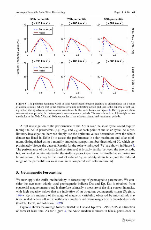
Figure 5 The potential economic value of solar-wind speed forecasts (relative to climatology) for a rangeof cost/loss ratios, where cost is the expense of taking mitigating action and loss is the expense of not tak-ing action during adverse space-weather conditions. In the same format as Figure 4. The top panels showsolar-maximum periods, the bottom panels solar-minimum periods. The rows show from left to right actionthresholds at the 50th, 75th, and 90th percentiles of the solar-maximum and -minimum periods.

A full investigation of the performance of the AnEn over the solar cycle would requiretuning the AnEn parameters (e.g. NEN and TT) at each point of the solar cycle. As a pre-liminary investigation, here we simply use the optimum values determined over the wholedataset (as listed in Table 1) to assess the performance in solar maximum and solar mini-mum, distinguished using a monthly smoothed sunspot-number threshold of 50, which ap-proximately bisects the dataset. Results for the solar-wind speed [VR] are shown in Figure 5.The performance of the AnEn (and persistence) is broadly similar between the two periods,but, somewhat counterintuitively, the AnEn appears to perform marginally better during so-lar maximum. This may be the result of reduced VR variability at this time (note the reducedrange of the percentiles in solar maximum compared with solar minimum).

5. Geomagnetic Forecasting

We now apply the AnEn methodology to forecasting of geomagnetic parameters. We con-sider the two most widely used geomagnetic indices: Dst and Kp. Dst is obtained fromequatorial magnetometers and is therefore primarily a measure of the ring-current intensity,with high negative values that are indicative of an on-going geomagnetic storm (Sugiura,1964). Kp is a measure of the range of magnetic variability observed by mid-latitude sta-tions, scaled between 0 and 9, with larger numbers indicating magnetically disturbed periods(Bartels, Heck, and Johnston, 1939).

Figure 6 shows the average forecast RMSE in Dst and Kp over 1996 – 2015 as a functionof forecast lead time. As for Figure 3, the AnEn median is shown in black, persistence in

69 Page 12 of 16 M.J. Owens et al.

Figure 6 Average forecast RMSE over 1996 – 2015 as a function of forecast lead time for (a) Kp and (b) Dst.Black, red, and blue lines show the AnEn, persistence, and climatological forecasts, respectively.

red, and climatology in blue. For both AnEn forecasts, the training window is 6 hours andthe number of ensemble members is 100. The analogues are determined purely from theforecast parameters (i.e. just Dst for the Dst forecast and just Kp for the Kp forecast). Whenwe use the current AnEn methodology, the inclusion of BN and/or VR as training parametersis found to produce little to no improvement in the forecast RMSE.

All forecasts show a strong diurnal variation in RMSE, resulting from the tilt of theEarth’s rotational axis relative to the Ecliptic plane, which leads to a diurnal variation in thecoupling efficiency between the heliospheric and magnetospheric magnetic fields (Siscoeand Crooker, 1996). Consequently, the best forecast (i.e. lowest RMSE) within a given 24-hour range of lead times occurs at the same time of day as the time the forecast is made(i.e. 0:00 UT in this case). For both Dst and Kp, persistence provides a better forecast thanclimatology out to around 24 hours lead time. The AnEn median provides a lower RMSE atall lead times beyond one hour and continues to provide a useful forecast out to around fourdays. In fact, the ability of the AnEn to select an appropriate climatology means it providesa better forecast than a simple climatological means for all lead times. Both persistence andthe AnEn median show a decrease in forecast RMSE for forecast lead times of around 27days, as expected.

The performance of the probabilistic AnEn is assessed in Figure 7. The potential eco-nomic value of acting on the 24-hour lead-time AnEn and persistence forecasts of Dst andKp are shown in the top and bottom rows, respectively. The AnEn forecast is comparable to,or better than, persistence for all thresholds and cost/loss ratios for both Dst and Kp, demon-strating the value of this approach for forecasting geomagnetic disturbances. The level ofimprovement provided by the AnEn over persistence, however, is a strong function of thecost/loss ratio, which is fixed by the application. So the benefit provided by the use of theAnEn will be strongly application dependent. These results also confirm that the AnEn pro-vides a useful measure of the forecast uncertainty, as well as the most probable value. Wealso note that relative to climatology, Dst appears to be far more predictable via both theAnEn and persistence than Kp.

Analogue Ensemble Solar Wind Forecasting Page 13 of 16 69

Figure 7 The potential economic value of a forecast (relative to climatology) for a range of cost/loss ratios,where cost is the expense of taking mitigating action and loss is the expense of not taking action duringadverse space-weather conditions. Red lines show the AnEn, blue dashed lines show persistence. The top rowshows the Dst forecast, the bottom row the Kp forecast. The columns show from left to right an increasingthreshold for taking action, namely the 50th, 75th, and 90th percentile of the forecast parameter.

6. Summary and Conclusions

We have investigated the use of an analogue ensemble (AnEn), often referred to as a “simi-lar day” approach, for probabilistic solar-wind and geomagnetic forecasting. This forecast isconstructed by determining a number of periods in the historical data that are “analogous” tothe current conditions. It is then assumed that future variations will follow the same trendsas these analogues. If an ensemble of analogues is used, the forecast is inherently proba-bilistic. As outlined by Riley et al. (2017), the AnEn approach is very promising for shortor medium lead-time solar-wind and geomagnetic forecasting (hours to days) and thus mayserve as a complementary approach to the longer lead-time (days to weeks) physics-basedmagnetohydrodynamic models.

Forecasts for four solar-wind parameters were considered, chosen for their geomagneticrelevance. They are the solar-wind radial speed [VR], the solar-wind density [NP], the merid-ional magnetic-field component in heliographic coordinates [BN] (which is approximatelythe southward magnetic field [BZ] in geocentric-solar-ecliptic, GSE, coordinates), and thetangential magnetic field [BT] (which is approximately BY in GSE coordinates).

A six-month interval of solar-wind data from the first half of 2003, including both ambi-ent solar wind and transient structures from coronal mass ejections, was used to determinethe optimum AnEn parameters. One of the most critical parameters is the length of the“training window” over which historical analogues are compared to current solar-wind con-ditions. In general, we found that around 6 – 12 hours was the optimum value in terms ofminimising the root mean-square error (RMSE) of the AnEn median. Increasing the length

69 Page 14 of 16 M.J. Owens et al.

of the training window beyond around 24 hours generally increased the RMSE of the result-ing forecast, as it reduces the number of suitable analogues in the historical dataset. As thesuitability of analogues decreases, the ensemble median forecast essentially reduces to cli-matology. A longer training window also decreases the relative weighting of the most recentobservations, which may produce less suitable analogues for future variations. The AnEnRMSE is also found to increase if the number of analogues in the ensemble is increasedabove around 100, as insufficient analogues are present in the currently available historicaldataset (around 60 years of near-Earth spacecraft observations). For solar-wind forecasting,the determination of the analogue periods was found to benefit from additional contextualinformation. For example, the AnEn VR forecast is improved when both VR and NP dataare considered in the training window, while the BN forecast improves when both BN andBT are considered. There is a trade-off, however, with increased specificity meaning thatthe number of suitable past analogues decreases and emphasis on the forecast parameter isreduced.

Using the optimal parameters, the AnEn forecasts were subsequently tested over a 19-year period of nearly complete solar-wind observational coverage, 1996 – 2015. As mostcommon space-weather metrics necessitate a deterministic forecast, it is instructive to firstreduce the AnEn to a deterministic forecast by considering only the median value. At veryshort forecast lead times (one to six hours), the high autocorrelation in the solar-wind plasmaparameters means that a persistence forecast of VR and NP is more accurate than the AnEnmedian or climatology. That advantage is rapidly lost with increasing lead time, with theAnEn median providing a much lower RMSE than persistence for lead times longer than afew hours. With increasing lead time, the RMSE of the AnEn grows, although at a slowerrate than persistence. For lead times longer than around 100 hours (approximately fourdays), the RMSE of the AnEn forecast of VR and NP plateaus, but to a value below cli-matology. This is due to the AnEn effectively selecting a more suitable “climatology” forthe forecast window than is given by simply averaging over the whole dataset, which canskew the mean towards, e.g., the wrong phase of the solar cycle.

Using the cost/loss method of determining the effectiveness of a probabilistic forecast,the 24-hour lead time AnEn forecast was shown to generally outperform persistence. ForBN, however, there is little value in the AnEn (or persistence) 24-hour lead-time forecastsrelative to climatology (i.e. BN = 0). When the lead time is reduced to three hours, however,the AnEn forecast has value, particularly for the extreme negative values that are of primeinterest to space-weather forecasting.

Finally, we considered the application of the AnEn to geomagnetic forecasting. The twomost commonly used geomagnetic indices, Dst and Kp, were considered. The AnEn ap-proach proved better than persistence for both indices over all forecast lead times and allcost/loss ratios.

7. Future Improvements

The solar-wind AnEn forecasts outlined in this study are by no means the best possible AnEnforecasts. Indeed, there should not be considered to be a single solar-wind AnEn, as forecastsshould be optimised for the required operational use. Some may emphasise a particularforecast lead time, some a more accurate “best” prediction, some a more accurate assessmentof the forecast uncertainty, etc. With this in mind, we outline a number of possible futureimprovements to solar-wind AnEn forecasting:

Analogue Ensemble Solar Wind Forecasting Page 15 of 16 69

– A more systematic exploration of the AnEn parameter space is required, ideally using alonger training dataset than the six months considered here. The limiting factor is compu-tation time.

– The AnEn parameterisation should be investigated using the cost/loss analysis, rather thanjust the RMSE of the AnEn median, in order to find the best probabilistic forecast. Thepotential issue is reducing the multi-dimensionality of the problem.

– Preliminary results suggest that stratifying the dataset by solar-cycle phase may help indistinguishing between solar-wind structures expected in the given forecast window, suchas corotating interaction regions in the declining phase of the solar-activity cycle.

– Only basic solar-wind parameters (plasma and magnetic field) were considered for de-termining the analogue periods, but other datasets may be able to give better contextualinformation. E.g. solar-wind compositional and charge-state data (e.g. Geiss, Gloeckler,and von Steiger, 1995; Lepri and Zurbuchen, 2004) may be useful for determining thesolar-wind types being encountered.

– Longer training windows (days to weeks) may be feasible and useful if the analogueperiods are weighted towards the most recent observations.

– Similarly, it may be helpful to use a greater number of solar-wind parameters in determin-ing the analogue periods if these training parameters can be accurately weighted towardsthe information that they contain for future variations of the forecast parameter (e.g. whenforecasting VR, it may be useful to determine the analogue periods on the basis of VR witha high weighting, NP with a medium weighting, and TP with a low weighting).

– In this study, past analogues were selected by minimising RMSE with the recent observa-tions. A more sophisticated pattern-matching or machine-learning algorithm may providea better AnEn forecast. This would essentially combine the neural network and AnEnapproaches.

Acknowledgements M. Owens is part-funded by Science and Technology Facilities Council (STFC) grantnumber ST/M000885/1 and acknowledges support from the Leverhulme Trust through a Philip LeverhulmePrize. The work has benefited from useful discussions as part of the NASA LWS-funded ProjectZed team.

Open Access This article is distributed under the terms of the Creative Commons Attribution 4.0 Inter-national License (http://creativecommons.org/licenses/by/4.0/), which permits unrestricted use, distribution,and reproduction in any medium, provided you give appropriate credit to the original author(s) and the source,provide a link to the Creative Commons license, and indicate if changes were made.

References

Bartels, J., Heck, N., Johnston, H.: 1939, Terr. Magn. Atmos. Electr. 44, 411.Boberg, F., Wintoft, P., Lundstedt, H.: 2000, Phys. Chem. Earth, Part C Solar-Terr. Planet. Sci. 25, 275. DOI.Bussy-Virat, C.D., Ridley, A.J.: 2016, Space Weather. DOI.Cannon, P., Angling, M., Barclay, L., Curry, C., Dyer, C., Edwards, R., et al.: 2013, Extreme Space Weather:

Impacts on Engineered Systems and Infrastructure, Royal Academy of Engineering, London.Cash, M.D., Biesecker, D.A., Pizzo, V., de Koning, C.A., Millward, G., Arge, C.N., et al.: 2015, Space

Weather 13, 611. DOI.Chen, J., Cargill, P.J., Palmadesso, P.J.: 1997, J. Geophys. Res. 102, 14701.Chree, C., Stagg, J.M.: 1928, Phil. Trans. Roy. Soc., Math. Phys. Eng. Sci. 227, 21. DOI.Delle Monache, L., Eckel, F.A., Rife, D.L., Nagarajan, B., Searight, K.: 2013, Mon. Weather Rev. 141, 3498.

DOI.Detman, T., Joselyn, J.: 1999, In: Habbal, S., Esser, R., Hollweg, J., Isenberg, P. (eds.) Solar Wind Nine

CP-471, AIP, Melville, 729.Dungey, J.W.: 1961, Phys. Rev. Lett. 6, 47.Geiss, J., Gloeckler, G., von Steiger, R.: 1995, Space Sci. Rev. 72, 49. DOI.

69 Page 16 of 16 M.J. Owens et al.

Hapgood, M.A.: 2011, Adv. Space Res. 47, 2059. DOI.King, J.H., Papitashvili, N.E.: 2005, J. Geophys. Res. 110, A02104. DOI.Lepri, S.T., Zurbuchen, T.H.: 2004, J. Geophys. Res. 109, A01112. DOI.Leutbecher, M., Palmer, T.N.: 2008, J. Comput. Phys. 227, 3515.Lockwood, M., Owens, M.J., Barnard, L.A., Bentley, S., Scott, C.J., Watt, C.E.: 2016, Space Weather 14,

406. DOI.Lorenz, E.N.: 1969, J. Atmos. Sci. 26, 636. DOI.Murphy, A.H.: 1977, Mon. Weather Rev. 105, 803.Odstrcil, D., Pizzo, V., Linker, J.A., Riley, P., Lionello, R., Mikic, Z.: 2004, J. Atmos. Solar-Terr. Phys. 66,

1311.Owens, M.J., Spence, H.E., McGregor, S., Hughes, W.J., Quinn, J.M., Arge, C.N., et al.: 2008, Space Weather

6, S08001. DOI.Owens, M.J., Challen, R., Methven, J., Henley, E., Jackson, D.R.: 2013, Space Weather 11, 225. DOI.Owens, M.J., Horbury, T.S., Wicks, R.T., McGregor, S.L., Savani, N.P., Xiong, M.: 2014, Space Weather 12,

395. DOI.Reikard, G.: 2016, NRIAG J. Astron. Geophys. DOI.Richardson, D.S.: 2000, Q. J. Roy. Meteorol. Soc. 126, 649.Riley, P., Linker, J.A., Mikic, Z.: 2001, J. Geophys. Res. 106, 15889.Riley, P., Ben Nun, M., Linker, J., Owens, M.J., Horbury, T.S.: 2017, Space Weather 15, 526. DOI.Rosenberg, R.L., Coleman, P.J.: 1969, J. Geophys. Res. 74, 5611.Russell, C., McPherron, R.: 1973, J. Geophys. Res. 78, 92.Siscoe, G., Crooker, N.: 1996, J. Geophys. Res. 101, 24985. DOI.Solares, J.R.A., Wei, H.-L., Boynton, R.J., Walker, S.N., Billings, S.A.: 2016, Space Weather 14, 899. DOI.Sugiura, M.: 1964, Hourly Values of Equatorial Dst for the IGY, Pergamon, Oxford.Tóth, G., Sokolov, I.V., Gombosi, T.I., Chesney, D.R., Clauer, C.R., De Zeeuw, D.L., et al.: 2005, J. Geophys.

Res. 110, A12226. DOI.van den Dool, H.M.: 1989, Mon. Weather Rev. 117, 2230. DOIWing, S., Johnson, J., Jen, J., Meng, C.I., Sibeck, D., Bechtold, K., et al.: 2005, J. Geophys. Res. 110, A04203.

DOI.