Embed Size (px)
Citation preview
Principles of
Quantum Computation and Quantum Information
Erwin BrüningSchool of Mathematical Sciences
April 2013
E. Brüning 2
Contents
1 Introduction 71.1 History . . . . . . . . . . . . . . . . . . . . . . . . . . . . . . . . . 81.2 Overview . . . . . . . . . . . . . . . . . . . . . . . . . . . . . . . . 11
2 Hilbert space QM 132.1 Hilbert spaces . . . . . . . . . . . . . . . . . . . . . . . . . . . . . 132.2 States and Observables . . . . . . . . . . . . . . . . . . . . . . . . 152.3 Time evolution . . . . . . . . . . . . . . . . . . . . . . . . . . . . . 182.4 Measurements . . . . . . . . . . . . . . . . . . . . . . . . . . . . . 19
2.4.1 General description of the measuring process . . . . . . 192.4.2 Born’s rule . . . . . . . . . . . . . . . . . . . . . . . . . . . 20
2.5 Measurements . . . . . . . . . . . . . . . . . . . . . . . . . . . . . 21
3
CONTENTS CONTENTS
2.6 Heisenberg’s Uncertainty Principle . . . . . . . . . . . . . . . . . 222.7 Composite systems and entanglement . . . . . . . . . . . . . . . 24
2.7.1 Measurements on entangled states . . . . . . . . . . . . . 26
3 Qubits and Quantum Circuits 313.1 Bits and Qubits . . . . . . . . . . . . . . . . . . . . . . . . . . . . 323.2 Quantum gates . . . . . . . . . . . . . . . . . . . . . . . . . . . . 37
3.2.1 Hadamard gate H . . . . . . . . . . . . . . . . . . . . . . 383.2.2 Pauli-X gate . . . . . . . . . . . . . . . . . . . . . . . . . . 393.2.3 Pauli-Y gate . . . . . . . . . . . . . . . . . . . . . . . . . . 393.2.4 Pauli-Z gate . . . . . . . . . . . . . . . . . . . . . . . . . . 403.2.5 Phase shift gates . . . . . . . . . . . . . . . . . . . . . . . 403.2.6 Swap gate . . . . . . . . . . . . . . . . . . . . . . . . . . . 403.2.7 Controlled gates . . . . . . . . . . . . . . . . . . . . . . . 413.2.8 Toffoli gate . . . . . . . . . . . . . . . . . . . . . . . . . . . 433.2.9 Fredkin gate . . . . . . . . . . . . . . . . . . . . . . . . . . 443.2.10 Example of an entangling circuit . . . . . . . . . . . . . . 45
4 Quantum Information Theory 47
E. Brüning 4
CONTENTS CONTENTS
4.1 Classical Information Theory . . . . . . . . . . . . . . . . . . . . 474.1.1 The case of two random variables . . . . . . . . . . . . . 504.1.2 Conditional Entropies and mutual Information . . . . . . 514.1.3 Channel capacity . . . . . . . . . . . . . . . . . . . . . . . 55
4.2 Quantum Information Theory . . . . . . . . . . . . . . . . . . . . 564.2.1 Quantum samples . . . . . . . . . . . . . . . . . . . . . . 564.2.2 Compatible and incompatible quantum samples . . . . . 574.2.3 Mutually-unbiased quantum samples . . . . . . . . . . . 584.2.4 Quantum channels . . . . . . . . . . . . . . . . . . . . . . 584.2.5 von Neumann entropy . . . . . . . . . . . . . . . . . . . . 60
5 Teleportation 635.1 Fully entangled states . . . . . . . . . . . . . . . . . . . . . . . . . 635.2 Dense Coding . . . . . . . . . . . . . . . . . . . . . . . . . . . . . 665.3 Teleportation . . . . . . . . . . . . . . . . . . . . . . . . . . . . . . 685.4 No Cloning . . . . . . . . . . . . . . . . . . . . . . . . . . . . . . . 75
6 Quantum Cryptography 796.1 The BB84 Scheme . . . . . . . . . . . . . . . . . . . . . . . . . . . 81
E. Brüning 5
CONTENTS CONTENTS
6.2 Ekert’s protocol E91 . . . . . . . . . . . . . . . . . . . . . . . . . . 896.3 Commercial implementations . . . . . . . . . . . . . . . . . . . . 93
7 Shor Factorization 977.1 Mathematical background . . . . . . . . . . . . . . . . . . . . . . 100
7.1.1 Some number theory . . . . . . . . . . . . . . . . . . . . . 1007.1.2 Quantum Fourier transform . . . . . . . . . . . . . . . . . 104
7.2 Reduction to period finding . . . . . . . . . . . . . . . . . . . . . 1097.3 Shor’s quantum algorithm . . . . . . . . . . . . . . . . . . . . . . 113
8 Other important Topics 1198.1 Deutsch: Universal Quantum Computer . . . . . . . . . . . . . . 1198.2 Grover’s search algorithm for unsorted database . . . . . . . . . 1198.3 Quantum Error Correction . . . . . . . . . . . . . . . . . . . . . . 1198.4 Quantum Complexity Theory . . . . . . . . . . . . . . . . . . . . 1198.5 Continuous variable QKD . . . . . . . . . . . . . . . . . . . . . . 1198.6 Physical Implementations . . . . . . . . . . . . . . . . . . . . . . 120
8.6.1 DiVincenzo Criteria . . . . . . . . . . . . . . . . . . . . . 1208.6.2 Possible qubits . . . . . . . . . . . . . . . . . . . . . . . . 122
E. Brüning 6
Chapter 1
Introduction
Quantum computation and quantum information is a quite recent and veryrapidly developing field of research. Effectively this field is based on funda-mental ideas from the following fields:
1. quantum mechanics; 2. computer science;
3. information theory; 4. cryptography.
Accordingly quantum computation and quantum information is an interdis-ciplinary field with ground breaking developments in the experimental andtheoretical side. It is based on profound experimental and theoretical progressin quantum physics (2012 Physics Nobel price winners: S. Haroche and D.
7
1.1. HISTORY CHAPTER 1. INTRODUCTION
Wineland: made tremendous advances in our understanding of quantum en-tanglement, with beautiful experiments to show how atomic systems can bemanipulated to exhibit the most extraordinary coherence properties).
Quantum computation requires some knowledge of the working of a classi-cal computer. But this will not be discussed here.
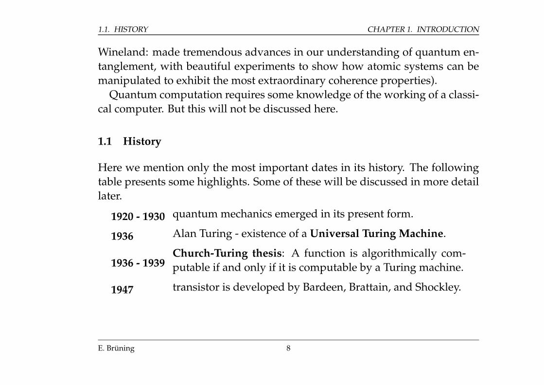
1.1 History
Here we mention only the most important dates in its history. The followingtable presents some highlights. Some of these will be discussed in more detaillater.
1920 - 1930 quantum mechanics emerged in its present form.
1936 Alan Turing - existence of a Universal Turing Machine.
1936 - 1939Church-Turing thesis: A function is algorithmically com-putable if and only if it is computable by a Turing machine.
1947 transistor is developed by Bardeen, Brattain, and Shockley.
E. Brüning 8
CHAPTER 1. INTRODUCTION 1.1. HISTORY
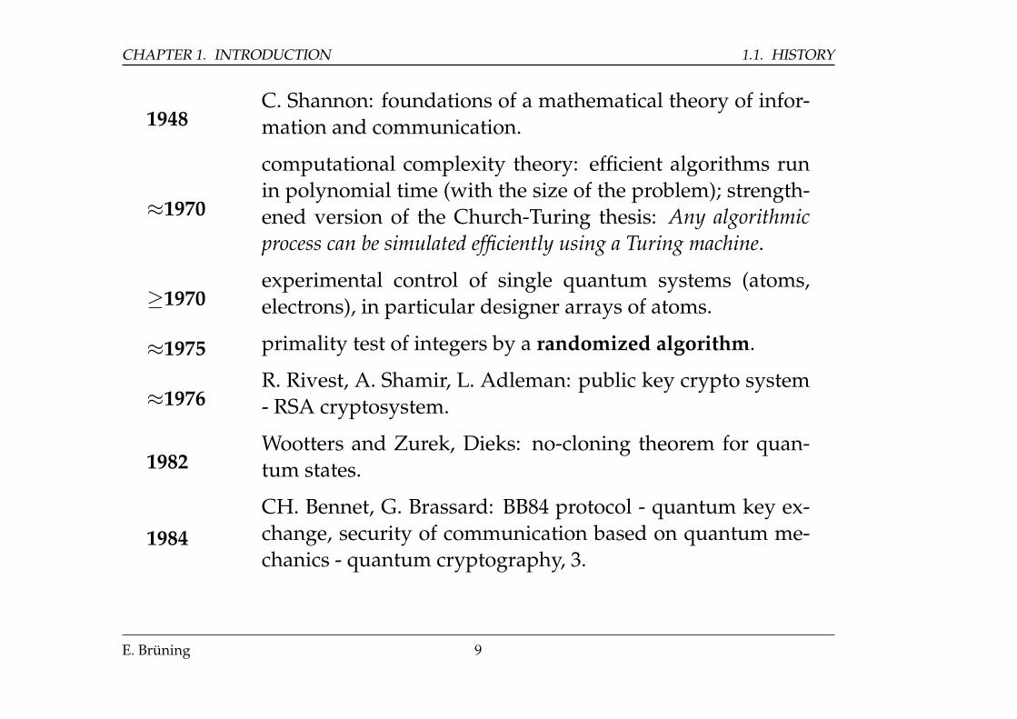
1948C. Shannon: foundations of a mathematical theory of infor-mation and communication.
≈1970
computational complexity theory: efficient algorithms runin polynomial time (with the size of the problem); strength-ened version of the Church-Turing thesis: Any algorithmicprocess can be simulated efficiently using a Turing machine.
≥1970experimental control of single quantum systems (atoms,electrons), in particular designer arrays of atoms.
≈1975 primality test of integers by a randomized algorithm.
≈1976R. Rivest, A. Shamir, L. Adleman: public key crypto system- RSA cryptosystem.
1982Wootters and Zurek, Dieks: no-cloning theorem for quan-tum states.
1984CH. Bennet, G. Brassard: BB84 protocol - quantum key ex-change, security of communication based on quantum me-chanics - quantum cryptography, 3.
E. Brüning 9
1.1. HISTORY CHAPTER 1. INTRODUCTION
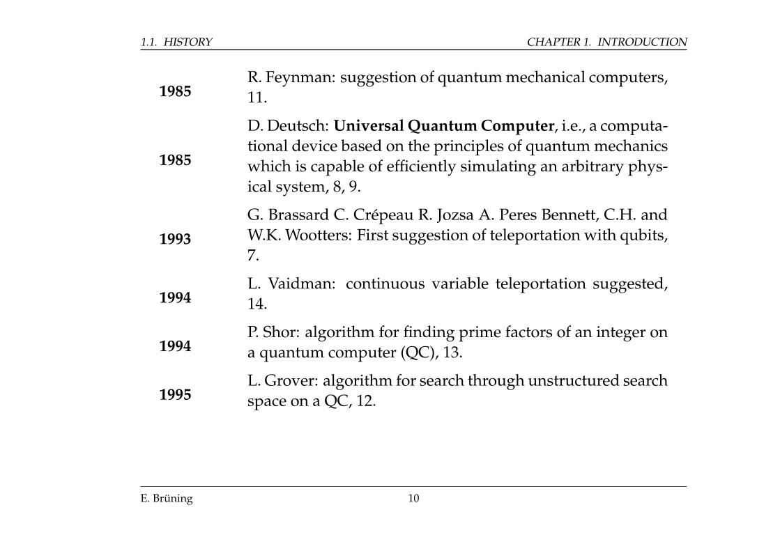
1985R. Feynman: suggestion of quantum mechanical computers,11.
1985
D. Deutsch: Universal Quantum Computer, i.e., a computa-tional device based on the principles of quantum mechanicswhich is capable of efficiently simulating an arbitrary phys-ical system, 8, 9.
1993G. Brassard C. Crépeau R. Jozsa A. Peres Bennett, C.H. andW.K. Wootters: First suggestion of teleportation with qubits,7.
1994L. Vaidman: continuous variable teleportation suggested,14.
1994P. Shor: algorithm for finding prime factors of an integer ona quantum computer (QC), 13.
1995L. Grover: algorithm for search through unstructured searchspace on a QC, 12.
E. Brüning 10
CHAPTER 1. INTRODUCTION 1.2. OVERVIEW
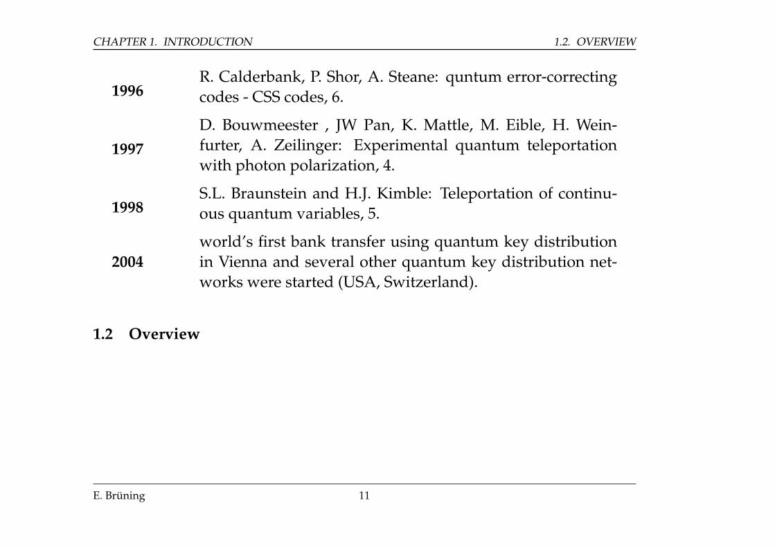
1996R. Calderbank, P. Shor, A. Steane: quntum error-correctingcodes - CSS codes, 6.
1997D. Bouwmeester , JW Pan, K. Mattle, M. Eible, H. Wein-furter, A. Zeilinger: Experimental quantum teleportationwith photon polarization, 4.
1998S.L. Braunstein and H.J. Kimble: Teleportation of continu-ous quantum variables, 5.
2004world’s first bank transfer using quantum key distributionin Vienna and several other quantum key distribution net-works were started (USA, Switzerland).
1.2 Overview
E. Brüning 11
1.2. OVERVIEW CHAPTER 1. INTRODUCTION
E. Brüning 12
Chapter 2
Quantum Mechanics in Hilbert space
In this chapter we recall briefly the basics of quantum mechanics in a form andin a notation used later.
2.1 Hilbert spaces
In the followingH denotes a complex separable Hilbert space. For most partsof this lecture H will actually be finite dimensional, i.e., isomorphic to theHilbert space of n-tuples of complex numbers, for n = 2,3, . . .:
H ' Cn.
13
2.1. HILBERT SPACES CHAPTER 2. HILBERT SPACE QM
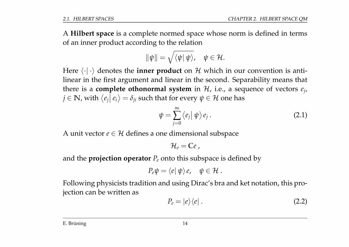
A Hilbert space is a complete normed space whose norm is defined in termsof an inner product according to the relation
‖ψ‖ =√〈ψ| ψ〉, ψ ∈ H.
Here 〈·| ·〉 denotes the inner product on H which in our convention is anti-linear in the first argument and linear in the second. Separability means thatthere is a complete othonormal system in H, i.e., a sequence of vectors ej,j ∈N, with
⟨ej∣∣ ei⟩= δji such that for every ψ ∈ H one has
ψ =∞
∑j=0
⟨ej∣∣ ψ⟩
ej . (2.1)
A unit vector e ∈ H defines a one dimensional subspace
He = Ce ,
and the projection operator Pe onto this subspace is defined by
Peψ = 〈e| ψ〉 e, ψ ∈ H .
Following physicists tradition and using Dirac’s bra and ket notation, this pro-jection can be written as
Pe = |e〉〈e| . (2.2)
E. Brüning 14
CHAPTER 2. HILBERT SPACE QM 2.2. STATES AND OBSERVABLES
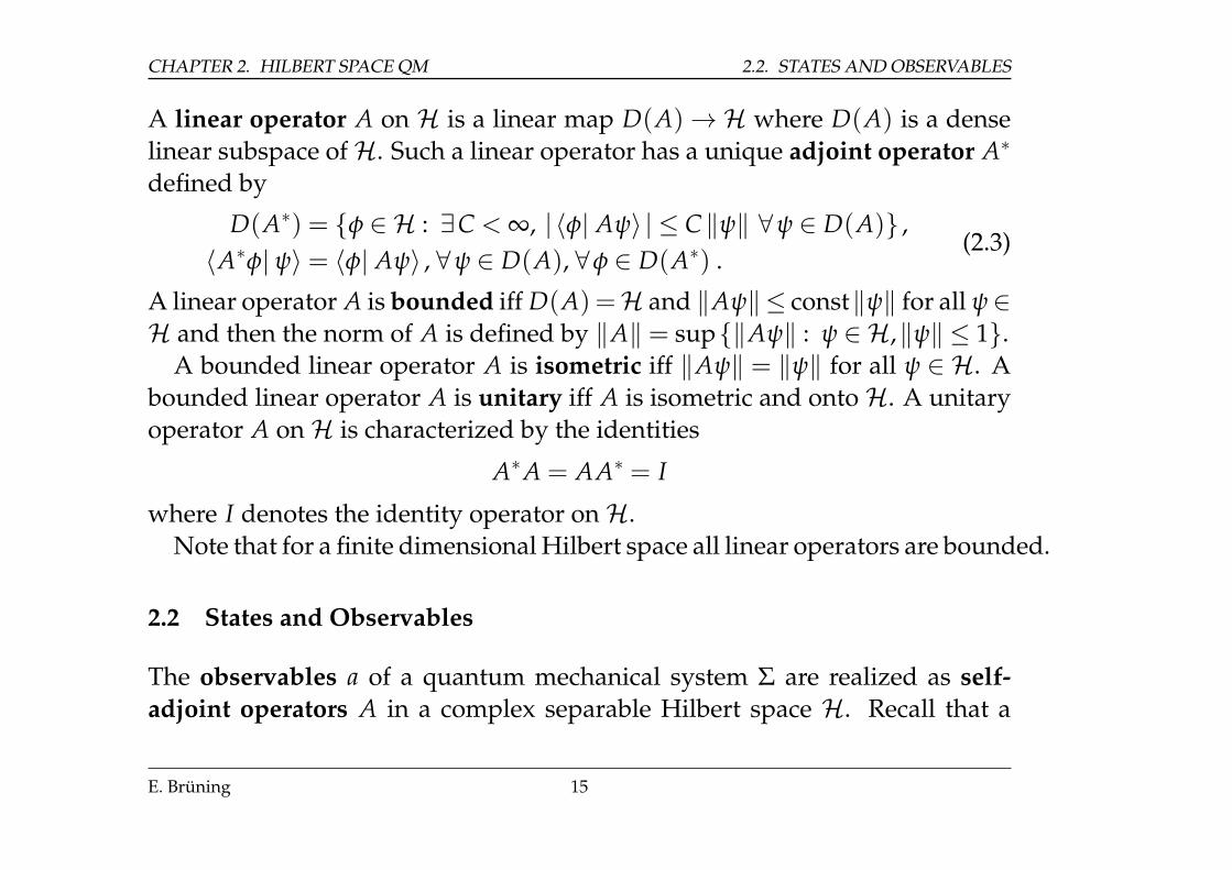
A linear operator A on H is a linear map D(A)→H where D(A) is a denselinear subspace ofH. Such a linear operator has a unique adjoint operator A∗
defined by
D(A∗) = {φ ∈ H : ∃C < ∞, | 〈φ| Aψ〉 | ≤ C‖ψ‖ ∀ψ ∈ D(A)} ,〈A∗φ| ψ〉 = 〈φ| Aψ〉 , ∀ψ ∈ D(A), ∀φ ∈ D(A∗) .
(2.3)
A linear operator A is bounded iff D(A) =H and ‖Aψ‖ ≤ const‖ψ‖ for all ψ∈H and then the norm of A is defined by ‖A‖ = sup{‖Aψ‖ : ψ ∈ H,‖ψ‖ ≤ 1}.
A bounded linear operator A is isometric iff ‖Aψ‖ = ‖ψ‖ for all ψ ∈ H. Abounded linear operator A is unitary iff A is isometric and onto H. A unitaryoperator A onH is characterized by the identities
A∗A = AA∗ = I
where I denotes the identity operator onH.Note that for a finite dimensional Hilbert space all linear operators are bounded.
2.2 States and Observables
The observables a of a quantum mechanical system Σ are realized as self-adjoint operators A in a complex separable Hilbert space H. Recall that a
E. Brüning 15
2.2. STATES AND OBSERVABLES CHAPTER 2. HILBERT SPACE QM
linear operator A is called self-adjoint iff it equals its adjoint: A = A∗ (note thatthis equality includes the equality of the domains of definition, i.e., D(A) =D(A∗) as defined above).
Many observables have to be realized by unbounded self-adjoint operators,for instance the momentum operator P or the energy operator or HamiltonianH.
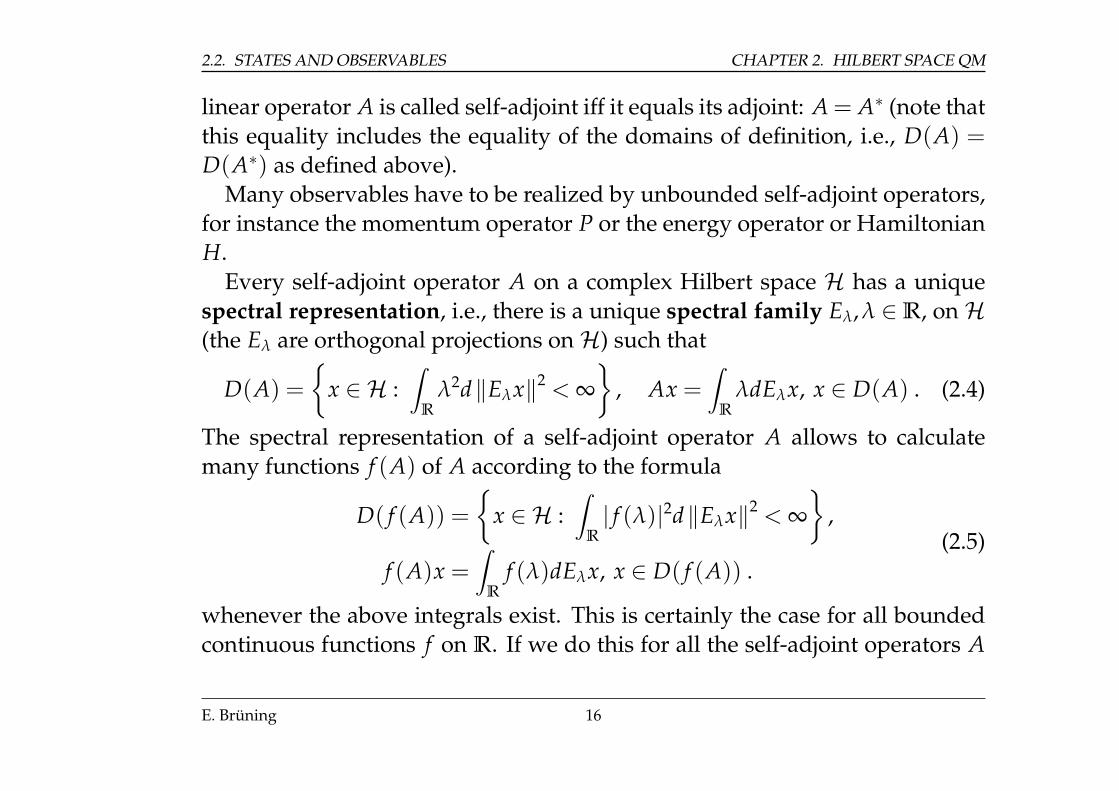
Every self-adjoint operator A on a complex Hilbert space H has a uniquespectral representation, i.e., there is a unique spectral family Eλ,λ ∈R, on H(the Eλ are orthogonal projections onH) such that
D(A) =
{x ∈ H :
∫R
λ2d‖Eλx‖2 < ∞}
, Ax =∫
R
λdEλx, x ∈ D(A) . (2.4)
The spectral representation of a self-adjoint operator A allows to calculatemany functions f (A) of A according to the formula
D( f (A)) =
{x ∈ H :
∫R
| f (λ)|2d‖Eλx‖2 < ∞}
,
f (A)x =∫
R
f (λ)dEλx, x ∈ D( f (A)) .(2.5)
whenever the above integrals exist. This is certainly the case for all boundedcontinuous functions f on R. If we do this for all the self-adjoint operators A
E. Brüning 16
CHAPTER 2. HILBERT SPACE QM 2.2. STATES AND OBSERVABLES
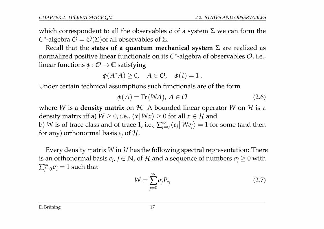
which correspondent to all the observables a of a system Σ we can form theC∗-algebra O =O(Σ)of all observables of Σ.
Recall that the states of a quantum mechanical system Σ are realized asnormalized positive linear functionals on its C∗-algebra of observables O, i.e.,linear functions φ :O→ C satisfying
φ(A∗A) ≥ 0, A ∈ O, φ(I) = 1 .
Under certain technical assumptions such functionals are of the form
φ(A) = Tr (WA), A ∈ O (2.6)
where W is a density matrix on H. A bounded linear operator W on H is adensity matrix iff a) W ≥ 0, i.e., 〈x|Wx〉 ≥ 0 for all x ∈ H andb) W is of trace class and of trace 1, i.e., ∑∞
j=0⟨ej∣∣Wej
⟩= 1 for some (and then
for any) orthonormal basis ej ofH.
Every density matrix W inH has the following spectral representation: Thereis an orthonormal basis ej, j ∈N, of H and a sequence of numbers σj ≥ 0 with∑∞
j=0 σj = 1 such that
W =∞
∑j=0
σjPej (2.7)
E. Brüning 17
2.3. TIME EVOLUTION CHAPTER 2. HILBERT SPACE QM
where Pej denotes the orthogonal projector onto the subspace spanned by thevector ej as given in (2.2). Note that some of the eigen-values σj of W can be 0.For such a W Formula (2.6) takes the form
φ(A) =∞
∑j=0
σj⟨ej∣∣ Aej
⟩(2.8)
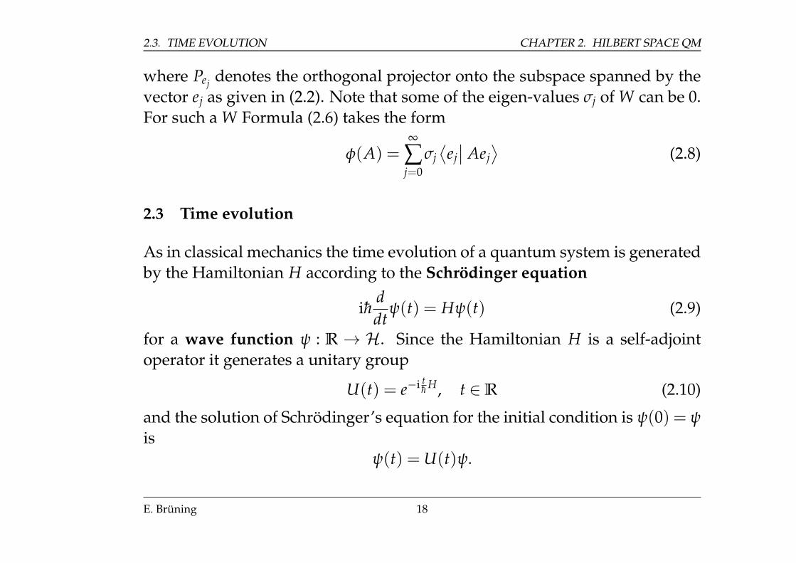
2.3 Time evolution
As in classical mechanics the time evolution of a quantum system is generatedby the Hamiltonian H according to the Schrödinger equation
ih̄ddt
ψ(t) = Hψ(t) (2.9)
for a wave function ψ : R→ H. Since the Hamiltonian H is a self-adjointoperator it generates a unitary group
U(t) = e−i th̄ H, t ∈R (2.10)
and the solution of Schrödinger’s equation for the initial condition is ψ(0) = ψ
isψ(t) = U(t)ψ.
E. Brüning 18
CHAPTER 2. HILBERT SPACE QM 2.4. MEASUREMENTS
In our context the Hamiltonian is always time independent and usually wework in units where h̄ = Planck’s constant
2π = 1. Note that
U(t)∗ = U(−t), U(t1)U(t2) = U(t1 + t2), U(0) = I
holds.
2.4 Measurements
2.4.1 General description of the measuring process
All the information which we have about a physical system is obtained fromobservations and measurements. Observations consist in bringing the systemunder examination in contact with some other system, the observer, or somemeasuring device M, and observing the reaction of the system on the observer.
Two important features of the measuring process:1. Back-effect of the measuring device on the system: The measuring device Mmust interact somehow with the system. But an interaction always acts bothways, hence M also acts on the system, producing an effect on the system withno particularly desirable consequences. This back-effect on the system seemsto be the cause of the difficulty in the interpretation of quantum mechanics.
E. Brüning 19
2.4. MEASUREMENTS CHAPTER 2. HILBERT SPACE QM
2. Appearance of the “conscious observer": If a measurement is to be usefulthere must be a further observation on M, namely “reading the scale". Suchfurther observations may be made at a later time by examining a permanentrecord of some sort, but in any case, these further observations must enterthe consciousness of a scientific observer. (Schrödinger: Knowledge whichnobody has, is no knowledge!)
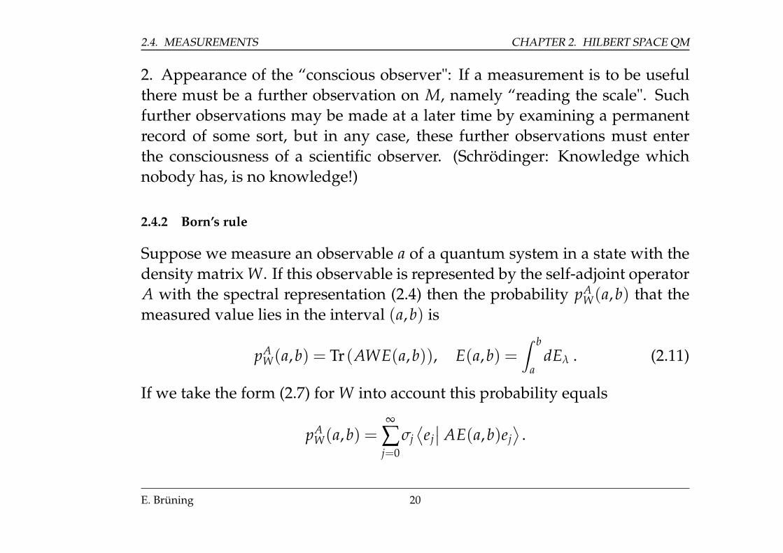
2.4.2 Born’s rule
Suppose we measure an observable a of a quantum system in a state with thedensity matrix W. If this observable is represented by the self-adjoint operatorA with the spectral representation (2.4) then the probability pA
W(a,b) that themeasured value lies in the interval (a,b) is
pAW(a,b) = Tr (AWE(a,b)), E(a,b) =
∫ b
adEλ . (2.11)
If we take the form (2.7) for W into account this probability equals
pAW(a,b) =
∞
∑j=0
σj⟨ej∣∣ AE(a,b)ej
⟩.
E. Brüning 20
CHAPTER 2. HILBERT SPACE QM 2.5. MEASUREMENTS
In particular, if the observable A has a purely discrete spectrum, i.e., A =
∑i aiPi and the system is in the pure state given by the unit vector ψ ∈ H, thenthis probability is
pAW(a,b) = ∑
ai∈(a,b)
ai 〈ψ| Piψ〉 . (2.12)
2.5 Measurements
Born’s rule gives the probability for a specific measurement outcome. Butoften in quantum mechanics one also needs to know the post measurementstate of the system at which the measurement has been performed. We recallhere the basic rules which we are going to use later. We restrict ourselves tothe case of a finite dimensional state Hilbert spaceH.
For an orthonormal basis{
ej}
of H denote by [ej] = Pej the orthogonal pro-jector onto the one dimensional subspace spanned by the vector ej. Typicallythese basis vectors are the eigen-vectors of some self-adjoint operator inH, i.e.,of an observable. According to (2.12) the probability for the outcome j of themeasurement is
∥∥[ej]ψ∥∥2
=⟨ψ∣∣ [ej]ψ
⟩= |⟨ej∣∣ ψ⟩|2 if our system is in the pure
E. Brüning 21
2.6. HEISENBERG’S UNCERTAINTY PRINCIPLE CHAPTER 2. HILBERT SPACE QM
state ψ ∈ H and the state of the system after the measurement is
[ej]ψ⟨ψ∣∣ [ej]ψ
⟩ = ⟨ej∣∣ ψ⟩⟨
ψ∣∣ [ej]ψ
⟩ej . (2.13)
If our system is in a general state with density matrix W, then the post mea-surement state is
[ej]W[ej]
Tr([ej]W[ej]). (2.14)
2.6 Heisenberg’s Uncertainty Principle
This principle states that in a quantum system only one property of a pair ofconjugate properties can be known with certainty. Recall that conjugate proper-ties are represented by self-adjoint operators which do not commute. Heisen-berg formulated this principle originally for the position and momentum of aparticle. The operators of position Q and momentum P satisfy the commuta-tion relation
[Q, P] = QP− PQ ⊂ iI (2.15)where I denotes as usual the identity operator and where the symbol ⊂ ex-presses the fact that the above identity holds on a dense subspace of the Hilbert
E. Brüning 22
CHAPTER 2. HILBERT SPACE QM 2.6. HEISENBERG’S UNCERTAINTY PRINCIPLE
spaceH, not on all ofH, since (2.15) involves unbounded operators.The mean values or expected value of an observable A in a state W is
E(A,W) = Tr (AW) = 〈A〉W.
Here and in the following we assume that the operator products are of traceclass.
The uncertainty of an observable A in a state W then is defined as
∆W(A) =√
Tr(A2W)− 〈A〉2W.
Now using the observation that
(A, B)→ Tr(A∗BW)
defines a positive semi-definite sesquiliear form for which the Cauchy-Schwarzinequality holds one shows Heisenberg uncertainty principle in general form
12|Tr([A, B]W)| ≤ ∆W(A)∆W(B), (2.16)
hence in the case of position and momentum one has for a pure state ψ
12≤ ∆ψ(Q)∆ψ(P).
E. Brüning 23
2.7. COMPOSITE SYSTEMS AND ENTANGLEMENT CHAPTER 2. HILBERT SPACE QM
2.7 Composite systems and entanglement
Suppose that a quantum system Σ is composed of two subsystems Σi withrespective Hilbert spaces Hi, , i = 1,2. Then the Hilbert H of Σ is the (Hilbert)tensor product of the spacesH1 andH2:
H =H1⊗H2
Note that in this formula the symbol⊗ denotes the completion of the algebraictensor product of the vector spaces Hi. If ej ( fk) is an orthonormal basis of H1
(H2) then
H =H1⊗H2 =
{∞
∑j,k=1
cjkej ⊗ fk : cjk ∈ C,∞
∑j,k=1|cjk|2 < ∞
}, (2.17)
i.e.,H1⊗H2 is the Hilbert space with ej⊗ fk, j,k ∈N, as an orthonormal basis.Thus elements ψ ∈H are given by double series according to (2.17). However,according to a much used result, each element ψ ∈H has also a representationby a single series.Schmidt decomposition: For every ψ ∈ H there are non-negative numbers pn
E. Brüning 24
CHAPTER 2. HILBERT SPACE QM 2.7. COMPOSITE SYSTEMS AND ENTANGLEMENT
and orthonormal bases e′n ofH1 respectively f ′n ofH2 such that
ψ =∞
∑n=1
pne′n ⊗ f ′n,∞
∑n=1
p2n = ‖ψ‖
2 . (2.18)
States ψ ∈ H are called separable iff there are ψ1 ∈ H1 and ψ2 ∈ H2 such that
ψ = ψ1⊗ ψ2.
States ψ ∈ H are called inseparable or entangled iff they are not separable.Entanglement of two quantum systems occurs when these systems (for in-
stance photons, electrons, molecules) interact physically and then become sep-arated; the type of interaction is such that each resulting member of a pairis properly described by the same quantum mechanical description (state),which is indefinite in terms of important factors such as position, momentum,spin, polarization, etc.
The concept of entanglement was suggested by E. Schrödinger in a replyto the EPR paradox, a thought experiment by which Einstein, Podolsky andRosen claimed to prove that the quantum-mechanical description of physicalreality given by wave functions is not complete. Schrödinger stated:
I would not call [entanglement] one but rather the characteristic trait
E. Brüning 25
2.7. COMPOSITE SYSTEMS AND ENTANGLEMENT CHAPTER 2. HILBERT SPACE QM
of quantum mechanics, the one that enforces its entire departure fromclassical lines of thought.
Quantum systems can become entangled through various types of interac-tions (see section on methods below). If entangled, one object cannot be fullydescribed without considering the other(s). They remain in a quantum super-position and share a single quantum state until a measurement is made.
For example entanglement occurs when subatomic particles decay into otherparticles. These decay events obey the various conservation laws, and as a re-sult, pairs of particles can be generated so that they are in some specific quan-tum states. Thus, entanglement is an experimentally verified and acceptedproperty of nature. Non-locality and hidden variables are two proposed mech-anisms that enable the effects of entanglement. And, as we will learn later,entanglement is a (physical) resource, for instance for quantum teleportationand to superdense coding.
2.7.1 Measurements on entangled states
We conclude this chapter with an explicit demonstration of the amazing con-sequences of entanglement. Suppose that a two qubit system is in the (gen-
E. Brüning 26
CHAPTER 2. HILBERT SPACE QM 2.7. COMPOSITE SYSTEMS AND ENTANGLEMENT
eral) state
ψ = ∑i,j=0,1
αij|ij〉12, |ij〉12 = |i〉1⊗ |j〉2, ‖ψ‖2 = ∑i,j=0,1
|αij|2 = 1 (2.19)
where the subscripts 1,2 refer to qubit 1 and qubit 2. On such a two qubitsystem various measurements can be performed.
1. Before any measurement the state of this system is uncertain.
2. After the measurement the state of the system is certain, it is |00〉12, |01〉12,|10〉12, |11〉12, with probability |α00|2, |α01|2, |α10|2, or |α11|2.
3. What conclusions can be drawn when we observe only the first (or onlythe second) qubit? We expect the system to be left in an uncertain state, be-cause we did not measure the second qubit that can still be in a continuumof states.
4. The first qubit can be in the state
• |0〉1 with probability |α00|2 + |α01|2, or
• |1〉1 with probability |α10|2 + |α11|2.
E. Brüning 27
2.7. COMPOSITE SYSTEMS AND ENTANGLEMENT CHAPTER 2. HILBERT SPACE QM
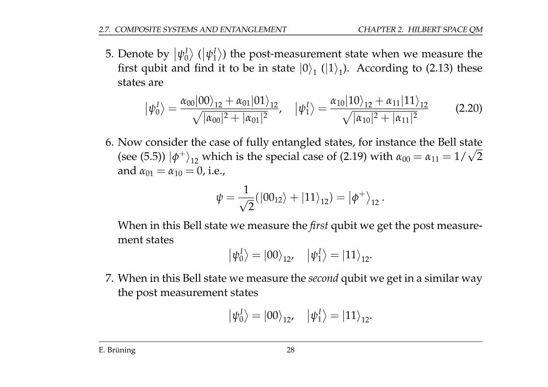
5. Denote by∣∣ψI
0
⟩(∣∣ψI
1
⟩) the post-measurement state when we measure the
first qubit and find it to be in state |0〉1 (|1〉1). According to (2.13) thesestates are∣∣ψI
0⟩=
α00|00〉12 + α01|01〉12√|α00|2 + |α01|2
,∣∣ψI
1⟩=
α10|10〉12 + α11|11〉12√|α10|2 + |α11|2
(2.20)
6. Now consider the case of fully entangled states, for instance the Bell state(see (5.5)) |φ+〉12 which is the special case of (2.19) with α00 = α11 = 1/
√2
and α01 = α10 = 0, i.e.,
ψ =1√2(|0012〉+ |11〉12) =
∣∣φ+⟩
12 .
When in this Bell state we measure the first qubit we get the post measure-ment states ∣∣ψI
0⟩= |00〉12,
∣∣ψI1⟩= |11〉12.
7. When in this Bell state we measure the second qubit we get in a similar waythe post measurement states∣∣ψI
0⟩= |00〉12,
∣∣ψI1⟩= |11〉12.
E. Brüning 28
CHAPTER 2. HILBERT SPACE QM 2.7. COMPOSITE SYSTEMS AND ENTANGLEMENT
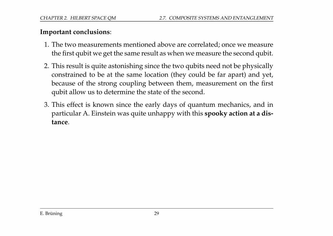
Important conclusions:
1. The two measurements mentioned above are correlated; once we measurethe first qubit we get the same result as when we measure the second qubit.
2. This result is quite astonishing since the two qubits need not be physicallyconstrained to be at the same location (they could be far apart) and yet,because of the strong coupling between them, measurement on the firstqubit allow us to determine the state of the second.
3. This effect is known since the early days of quantum mechanics, and inparticular A. Einstein was quite unhappy with this spooky action at a dis-tance.
E. Brüning 29
2.7. COMPOSITE SYSTEMS AND ENTANGLEMENT CHAPTER 2. HILBERT SPACE QM
E. Brüning 30
Chapter 3
Qubits and Quantum Circuits
In our lecture we assume that you have some background in classical comput-ers. In the 1930s C. Shannon studied switching circuits and observed that onecould apply the rules of Boole’s algebra in this setting and he introduced theconcept switching algebra as a way to analyze and design circuits by algebraicmeans in terms of logic gates.
Boolean algebra deals with the values 0 and 1 which can be thought of astwo integers, or as the truth values false and true respectively. They are calledbits or binary digits in contrast to the decimal digits 0,1, . . . ,9.
A logic gate is a device implementing a Boolean function, i.e., it performsa logical operation on one or more logical inputs and produces a single logic
31
3.1. BITS AND QUBITS CHAPTER 3. QUBITS AND QUANTUM CIRCUITS
output. Such gates are primarily implemented using diodes or transistors aselectronic switches. Logic gates can be put together to form compound logicgates or logic circuits, for instance in a present day computer.
In a classical computer the only reversible logic gate is the NOT gate. An n-bit datum is a string of bits x1, x2, . . . , xn of length n. They are stored in an n-bitregister. The set of n-bit data is the space {0,1}n which consists of 2n strings of0’s and 1’s. Thus we can formulate
An n-bit reversible gate is a bijective mapping f from the set {0,1}n
onto itself.
3.1 Bits and Qubits
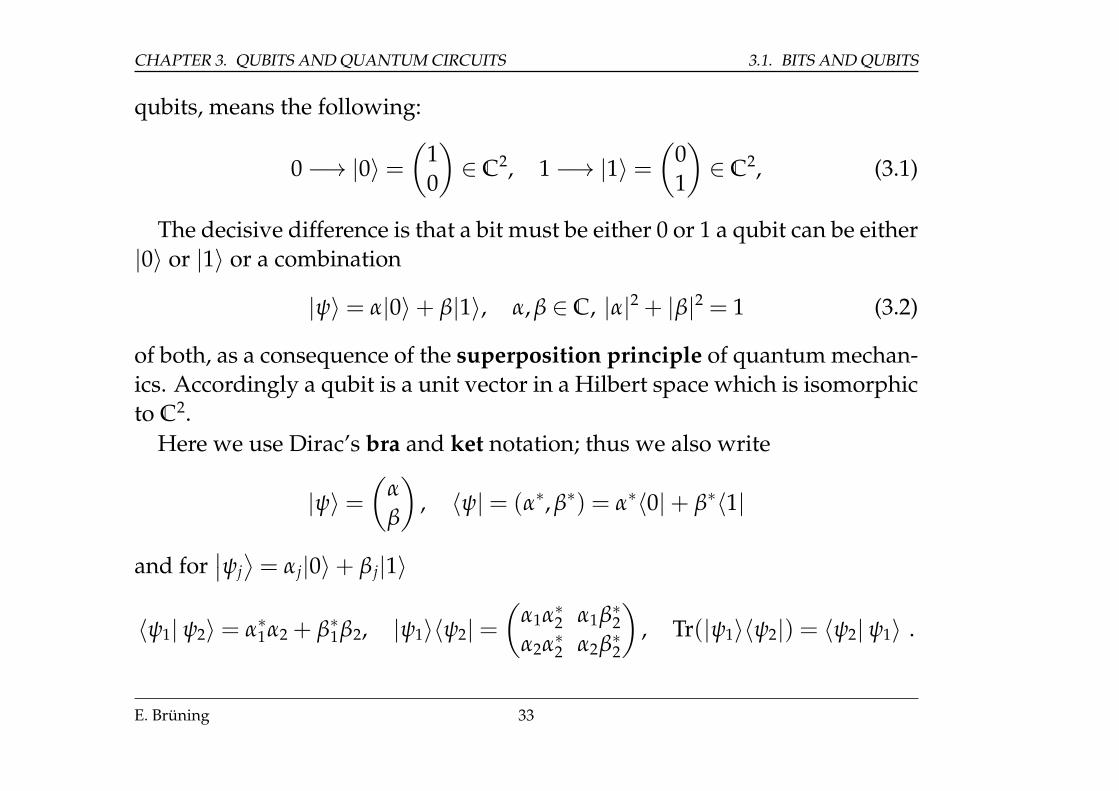
As a bit is the basic unit of classical computation and classical information aqubit or quantum bit is the basic unit of quantum computing and quantuminformation, realized as a two-state quantum mechanical system. The twostates in which a qubit may be measured are called basis states (or vectors)and traditionally are denoted as |0〉 and |1〉 (computational basis states).
The process of quantization in this context, i.e., the transition from bits to
E. Brüning 32
CHAPTER 3. QUBITS AND QUANTUM CIRCUITS 3.1. BITS AND QUBITS
qubits, means the following:
0−→ |0〉 =(
10
)∈ C2, 1−→ |1〉 =
(01
)∈ C2, (3.1)
The decisive difference is that a bit must be either 0 or 1 a qubit can be either|0〉 or |1〉 or a combination
|ψ〉 = α|0〉+ β|1〉, α, β ∈ C, |α|2 + |β|2 = 1 (3.2)
of both, as a consequence of the superposition principle of quantum mechan-ics. Accordingly a qubit is a unit vector in a Hilbert space which is isomorphicto C2.
Here we use Dirac’s bra and ket notation; thus we also write
|ψ〉 =(
α
β
), 〈ψ| = (α∗, β∗) = α∗〈0|+ β∗〈1|
and for∣∣ψj⟩= αj|0〉+ β j|1〉
〈ψ1| ψ2〉 = α∗1α2 + β∗1β2, |ψ1〉〈ψ2| =(
α1α∗2 α1β∗2α2α∗2 α2β∗2
), Tr(|ψ1〉〈ψ2|) = 〈ψ2| ψ1〉 .
E. Brüning 33
3.1. BITS AND QUBITS CHAPTER 3. QUBITS AND QUANTUM CIRCUITS
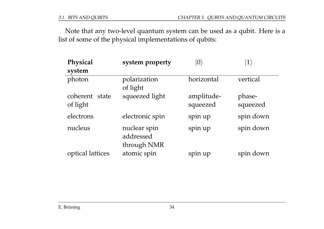
Note that any two-level quantum system can be used as a qubit. Here is alist of some of the physical implementations of qubits:
Physicalsystem
system property |0〉 |1〉
photon polarizationof light
horizontal vertical
coherent stateof light
squeezed light amplitude-squeezed
phase-squeezed
electrons electronic spin spin up spin down
nucleus nuclear spinaddressedthrough NMR
spin up spin down
optical lattices atomic spin spin up spin down
E. Brüning 34
CHAPTER 3. QUBITS AND QUANTUM CIRCUITS 3.1. BITS AND QUBITS
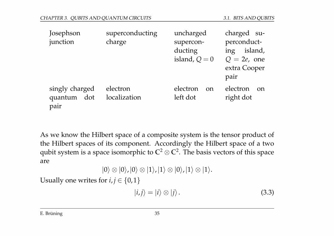
Josephsonjunction
superconductingcharge
unchargedsupercon-ductingisland, Q = 0
charged su-perconduct-ing island,Q = 2e, oneextra Cooperpair
singly chargedquantum dotpair
electronlocalization
electron onleft dot
electron onright dot
As we know the Hilbert space of a composite system is the tensor product ofthe Hilbert spaces of its component. Accordingly the Hilbert space of a twoqubit system is a space isomorphic to C2⊗C2. The basis vectors of this spaceare
|0〉 ⊗ |0〉, |0〉 ⊗ |1〉, |1〉 ⊗ |0〉, |1〉 ⊗ |1〉.Usually one writes for i, j ∈ {0,1}
|i, j〉 = |i〉 ⊗ |j〉 . (3.3)
E. Brüning 35
3.1. BITS AND QUBITS CHAPTER 3. QUBITS AND QUANTUM CIRCUITS
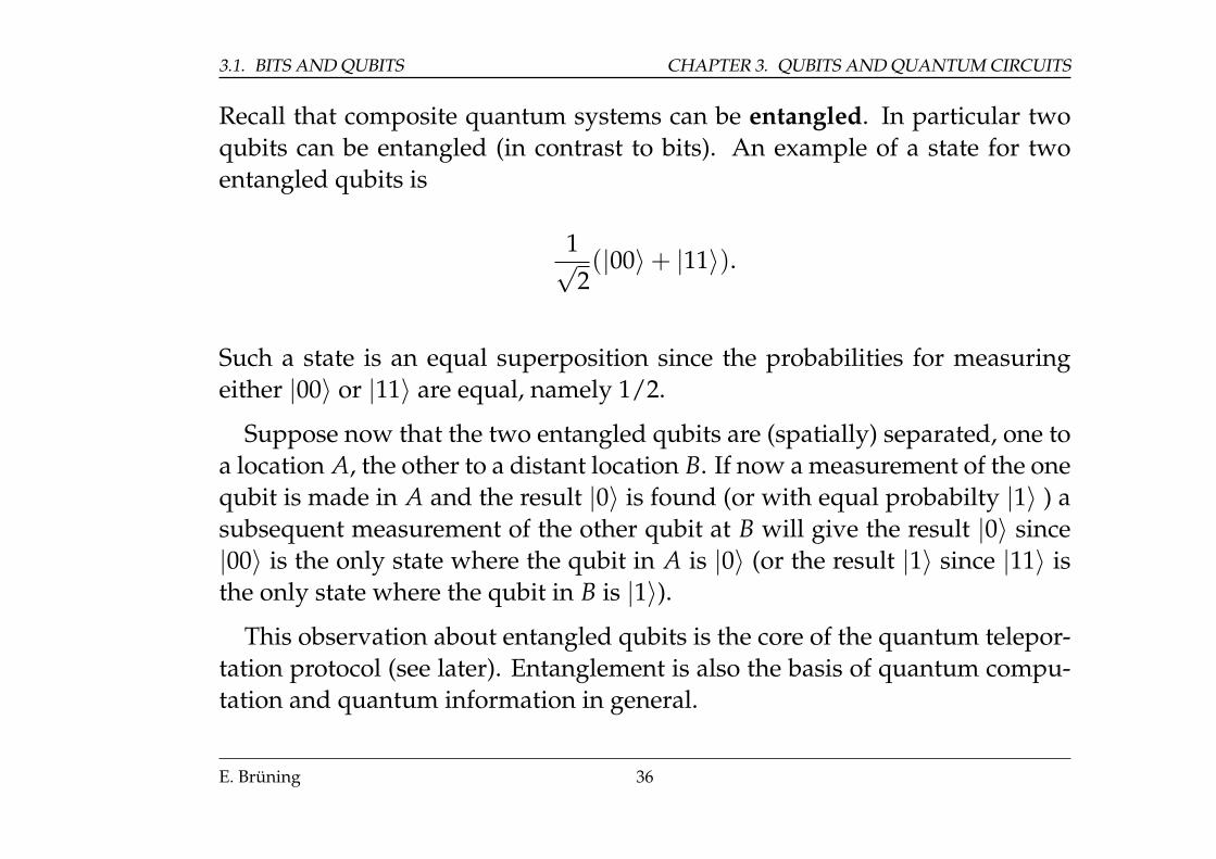
Recall that composite quantum systems can be entangled. In particular twoqubits can be entangled (in contrast to bits). An example of a state for twoentangled qubits is
1√2(|00〉+ |11〉).
Such a state is an equal superposition since the probabilities for measuringeither |00〉 or |11〉 are equal, namely 1/2.
Suppose now that the two entangled qubits are (spatially) separated, one toa location A, the other to a distant location B. If now a measurement of the onequbit is made in A and the result |0〉 is found (or with equal probabilty |1〉 ) asubsequent measurement of the other qubit at B will give the result |0〉 since|00〉 is the only state where the qubit in A is |0〉 (or the result |1〉 since |11〉 isthe only state where the qubit in B is |1〉).
This observation about entangled qubits is the core of the quantum telepor-tation protocol (see later). Entanglement is also the basis of quantum compu-tation and quantum information in general.
E. Brüning 36
CHAPTER 3. QUBITS AND QUANTUM CIRCUITS 3.2. QUANTUM GATES
3.2 Quantum gates
There are two basic operations on pure qubit states.
• A quantum logic gate operates on a qubit |ψ〉 and produces another qubit|ψ〉′. Mathematically this is realized by a unitary transformation of thestate space.
• Another operation on qubits is a standard basis measurement. The resultof such a measurement on (3.2) will be either |0〉 with probability |α|2 or|1〉 with probability |β|2.
Quantum logic gates are reversible, unlike many classical logic gates. How-ever classical computing can be done using only reversible gates, since it isknown that the reversible Toffoli gate (or CCNOT gate) can implement allBoolean functions. This controlled-controlled-not gate has a direct quantumequivalent, hence quantum circuits which are built out of quantum gates canperform all operations performed by classical logic circuits.
As indicated above quantum gates are represented by unitary matrices onthe corresponding Hilbert space. The Hilbert space for one qubit is C2, as thequantized version of the one bit space {0,1}. More generally the quantized
E. Brüning 37
3.2. QUANTUM GATES CHAPTER 3. QUBITS AND QUANTUM CIRCUITS
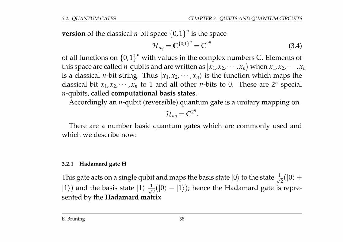
version of the classical n-bit space {0,1}n is the space
Hnq = C{0,1}n= C2n
(3.4)
of all functions on {0,1}n with values in the complex numbers C. Elements ofthis space are called n-qubits and are written as |x1, x2, · · · , xn〉when x1, x2, · · · , xn
is a classical n-bit string. Thus |x1, x2, · · · , xn〉 is the function which maps theclassical bit x1, x2, · · · , xn to 1 and all other n-bits to 0. These are 2n specialn-qubits, called computational basis states.
Accordingly an n-qubit (reversible) quantum gate is a unitary mapping on
Hnq = C2n.
There are a number basic quantum gates which are commonly used andwhich we describe now:
3.2.1 Hadamard gate H
This gate acts on a single qubit and maps the basis state |0〉 to the state 1√2(|0〉+
|1〉) and the basis state |1〉 1√2(|0〉 − |1〉); hence the Hadamard gate is repre-
sented by the Hadamard matrix
E. Brüning 38
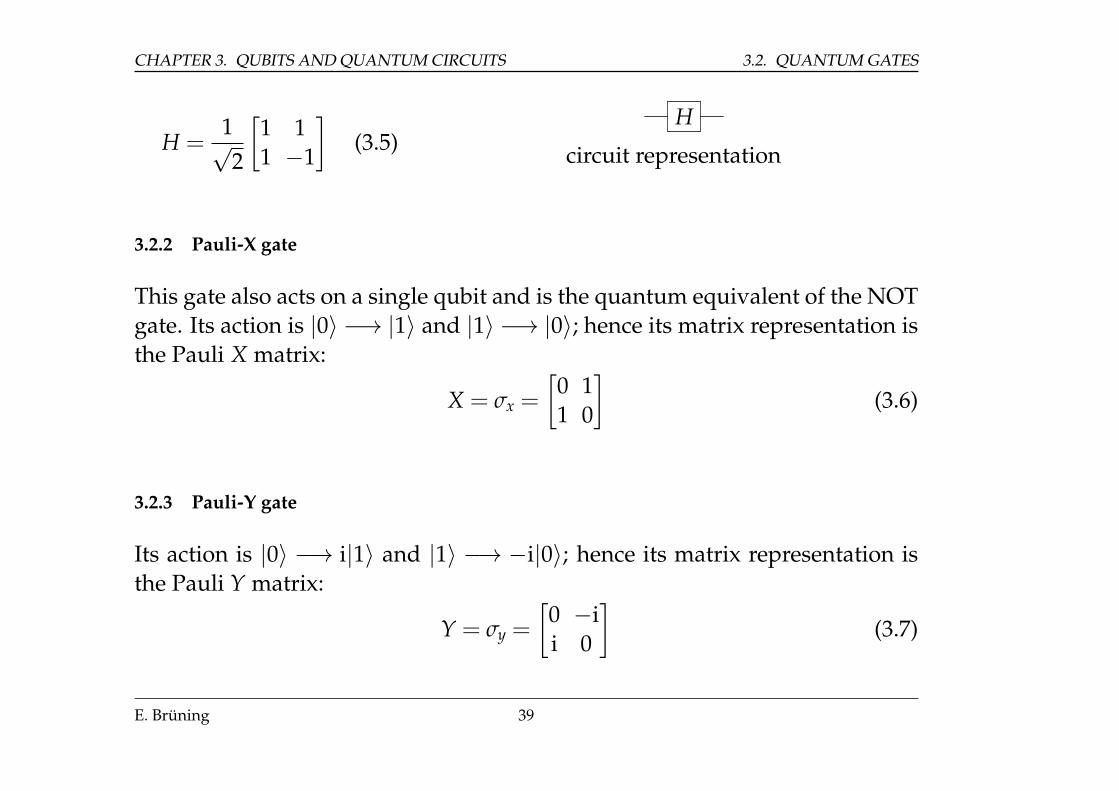
CHAPTER 3. QUBITS AND QUANTUM CIRCUITS 3.2. QUANTUM GATES
H =1√2
[1 11 −1
](3.5)
H
circuit representation
3.2.2 Pauli-X gate
This gate also acts on a single qubit and is the quantum equivalent of the NOTgate. Its action is |0〉 −→ |1〉 and |1〉 −→ |0〉; hence its matrix representation isthe Pauli X matrix:
X = σx =
[0 11 0
](3.6)
3.2.3 Pauli-Y gate
Its action is |0〉 −→ i|1〉 and |1〉 −→ −i|0〉; hence its matrix representation isthe Pauli Y matrix:
Y = σy =
[0 −ii 0
](3.7)
E. Brüning 39
3.2. QUANTUM GATES CHAPTER 3. QUBITS AND QUANTUM CIRCUITS
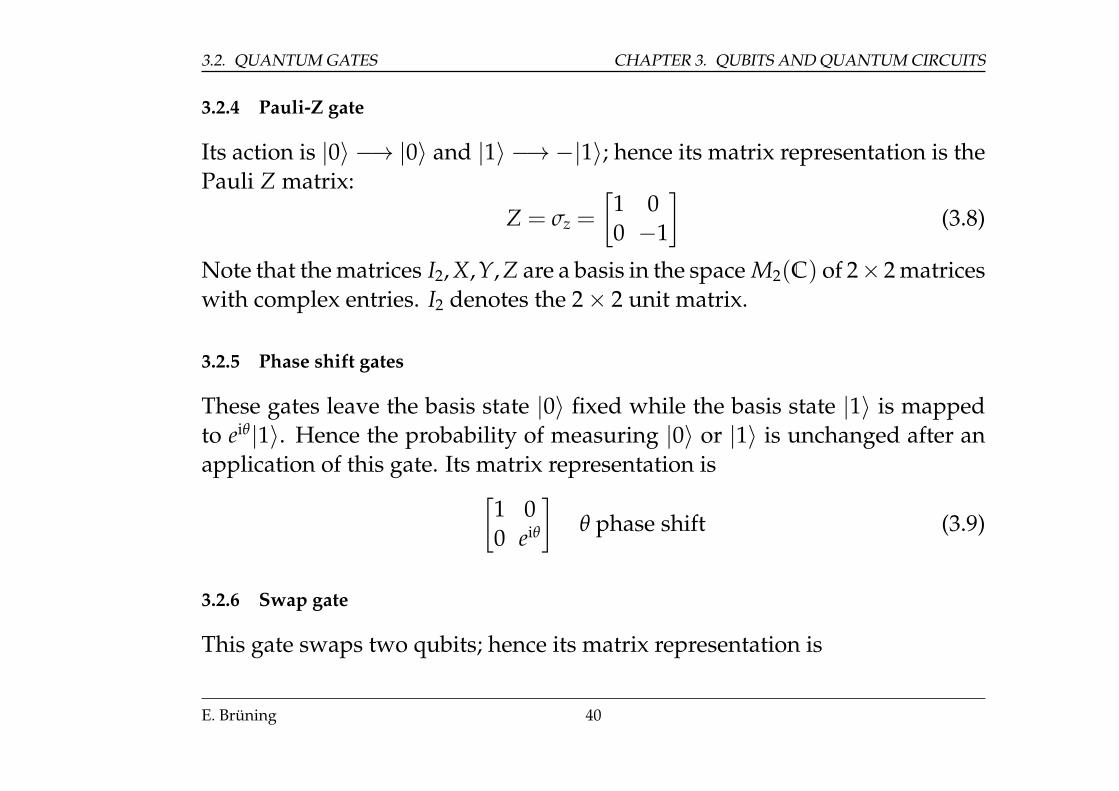
3.2.4 Pauli-Z gate
Its action is |0〉 −→ |0〉 and |1〉 −→−|1〉; hence its matrix representation is thePauli Z matrix:
Z = σz =
[1 00 −1
](3.8)
Note that the matrices I2, X,Y, Z are a basis in the space M2(C) of 2× 2 matriceswith complex entries. I2 denotes the 2× 2 unit matrix.
3.2.5 Phase shift gates
These gates leave the basis state |0〉 fixed while the basis state |1〉 is mappedto eiθ|1〉. Hence the probability of measuring |0〉 or |1〉 is unchanged after anapplication of this gate. Its matrix representation is[
1 00 eiθ
]θ phase shift (3.9)
3.2.6 Swap gate
This gate swaps two qubits; hence its matrix representation is
E. Brüning 40
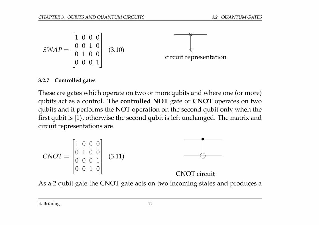
CHAPTER 3. QUBITS AND QUANTUM CIRCUITS 3.2. QUANTUM GATES
SWAP =
1 0 0 00 0 1 00 1 0 00 0 0 1
(3.10)
×
×circuit representation
3.2.7 Controlled gates
These are gates which operate on two or more qubits and where one (or more)qubits act as a control. The controlled NOT gate or CNOT operates on twoqubits and it performs the NOT operation on the second qubit only when thefirst qubit is |1〉, otherwise the second qubit is left unchanged. The matrix andcircuit representations are
CNOT =
1 0 0 00 1 0 00 0 0 10 0 1 0
(3.11)
•
CNOT circuitAs a 2 qubit gate the CNOT gate acts on two incoming states and produces a
E. Brüning 41
3.2. QUANTUM GATES CHAPTER 3. QUBITS AND QUANTUM CIRCUITS
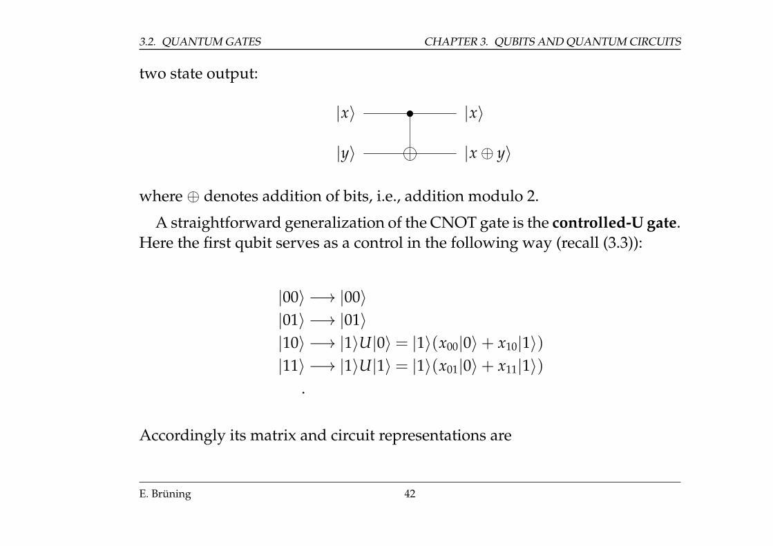
two state output:
|x〉 • |x〉
|y〉 |x⊕ y〉
where ⊕ denotes addition of bits, i.e., addition modulo 2.
A straightforward generalization of the CNOT gate is the controlled-U gate.Here the first qubit serves as a control in the following way (recall (3.3)):
|00〉 −→ |00〉|01〉 −→ |01〉|10〉 −→ |1〉U|0〉 = |1〉(x00|0〉+ x10|1〉)|11〉 −→ |1〉U|1〉 = |1〉(x01|0〉+ x11|1〉)
.
Accordingly its matrix and circuit representations are
E. Brüning 42
CHAPTER 3. QUBITS AND QUANTUM CIRCUITS 3.2. QUANTUM GATES
C(U) =
1 0 0 00 1 0 00 0 x00 x01
0 0 x10 x11
(3.12)
•
U
controlled -U gateThe circuit representation on two incoming states |x〉, |y〉 thus is
|x〉 • |x〉
|y〉 U Ux|y〉
The CNOT gate is the special case Ux = X.
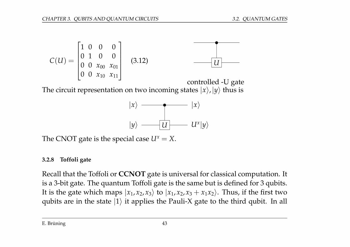
3.2.8 Toffoli gate
Recall that the Toffoli or CCNOT gate is universal for classical computation. Itis a 3-bit gate. The quantum Toffoli gate is the same but is defined for 3 qubits.It is the gate which maps |x1, x2, x3〉 to |x1, x2, x3 + x1x2〉. Thus, if the first twoqubits are in the state |1〉 it applies the Pauli-X gate to the third qubit. In all
E. Brüning 43
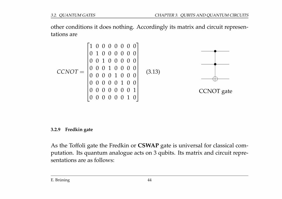
3.2. QUANTUM GATES CHAPTER 3. QUBITS AND QUANTUM CIRCUITS
other conditions it does nothing. Accordingly its matrix and circuit represen-tations are
CCNOT =
1 0 0 0 0 0 0 00 1 0 0 0 0 0 00 0 1 0 0 0 0 00 0 0 1 0 0 0 00 0 0 0 1 0 0 00 0 0 0 0 1 0 00 0 0 0 0 0 0 10 0 0 0 0 0 1 0
(3.13)
•
•
CCNOT gate
3.2.9 Fredkin gate
As the Toffoli gate the Fredkin or CSWAP gate is universal for classical com-putation. Its quantum analogue acts on 3 qubits. Its matrix and circuit repre-sentations are as follows:
E. Brüning 44
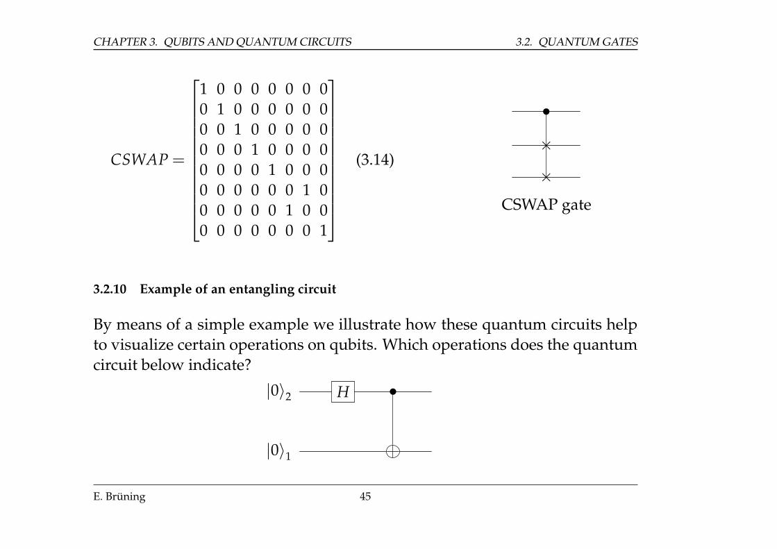
CHAPTER 3. QUBITS AND QUANTUM CIRCUITS 3.2. QUANTUM GATES
CSWAP =
1 0 0 0 0 0 0 00 1 0 0 0 0 0 00 0 1 0 0 0 0 00 0 0 1 0 0 0 00 0 0 0 1 0 0 00 0 0 0 0 0 1 00 0 0 0 0 1 0 00 0 0 0 0 0 0 1
(3.14)
•
×
×CSWAP gate
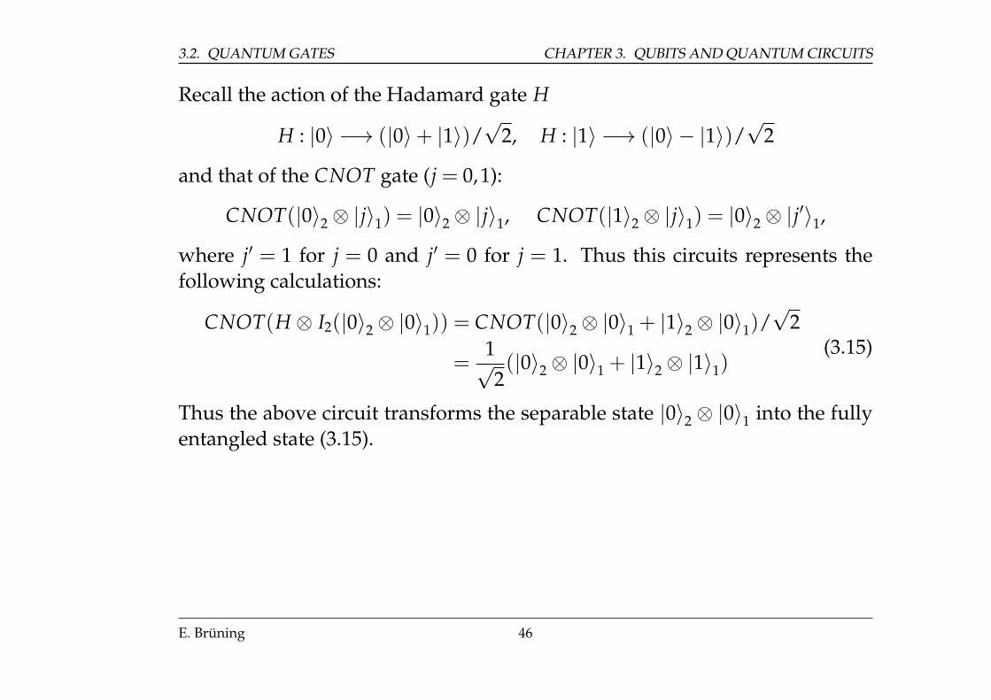
3.2.10 Example of an entangling circuit
By means of a simple example we illustrate how these quantum circuits helpto visualize certain operations on qubits. Which operations does the quantumcircuit below indicate?
|0〉2 H •
|0〉1
E. Brüning 45
3.2. QUANTUM GATES CHAPTER 3. QUBITS AND QUANTUM CIRCUITS
Recall the action of the Hadamard gate H
H : |0〉 −→ (|0〉+ |1〉)/√
2, H : |1〉 −→ (|0〉 − |1〉)/√
2
and that of the CNOT gate (j = 0,1):
CNOT(|0〉2⊗ |j〉1) = |0〉2⊗ |j〉1, CNOT(|1〉2⊗ |j〉1) = |0〉2⊗ |j′〉1,
where j′ = 1 for j = 0 and j′ = 0 for j = 1. Thus this circuits represents thefollowing calculations:
CNOT(H ⊗ I2(|0〉2⊗ |0〉1)) = CNOT(|0〉2⊗ |0〉1 + |1〉2⊗ |0〉1)/√
2
=1√2(|0〉2⊗ |0〉1 + |1〉2⊗ |1〉1)
(3.15)
Thus the above circuit transforms the separable state |0〉2 ⊗ |0〉1 into the fullyentangled state (3.15).
E. Brüning 46
Chapter 4
Quantum Information Theory
4.1 Classical Information Theory
Classical information theory as developed by C. Shannon and his successorsaddresses the following type of questions and suggests solutions.
Suppose a certain message is to be transmitted from a location A to a loca-tion B.
1. What resources are need for this transmission?
2. If we have a transmission channel with capacity of c bits per second, howlong will it take?
47
4.1. CLASSICAL INFORMATION THEORY CHAPTER 4. QUANTUM INFORMATION THEORY
3. If the transmission introduces errors (e.g. noise) what can be done aboutthis?
Recall that a string of n bits can represent N = 2n messages. Thus, for thetransmission of one of N distinct messages it is sensible to define the amountof information carried by a single message to be
log2 N bits.
But typically one has to transmit a message from a given collection of N mes-sages repeatedly, and if the messages can be assigned a non-uniform probabilitydistribution, then, on average it is possible to use fewer than log N bits persecond in order to transmit or store them.
Data compression (for instance ‘gzip‘) is a known method to store messagesefficiently. The key observation is to encode more common messages by usingshort strings of bits while less common message are encoded by longer strings.
The Shannon entropy is a logarithmic information measure, typically de-noted H(X) if X is a collection of labels x for a set of N messages. Supposethat p(x) is the probability for message x, with ∑x p(x) = 1. Or X is a ran-dom variable, i.e., a numerical function on some sample space; each x maycorrespond to several points in the sample space and p(x) is the sum of the
E. Brüning 48
CHAPTER 4. QUANTUM INFORMATION THEORY 4.1. CLASSICAL INFORMATION THEORY
probabilities associated with these points. Then one defines
H(X) = H(p) = −∑x
p(x) log2 p(x). (4.1)
Basic properties:
• H(X)≥ 0 and H(X) = 0 iff there is some x0 such that p(x0) = 1 and p(x) =0 for x 6= x0.
• If x can take only k values then H(X) ≤ logk and H(X) = logk iff p(x) =1/k for all x.
An intuitive interpretation of H(X) is the amount of information on averageconveyed by an observation of x. If x is a message, then H(X) is the averagemissing information about the message before it is received, and thus the aver-age information conveyed by the message, since after a message is received(and read), the missing information about this particular message is 0.
One can also think of H(X) as the difference, on average, of the informationpossessed by someone who knows what the actual message is, over againstsomeone who knows the probability distribution but does not know the mes-sage.
E. Brüning 49
4.1. CLASSICAL INFORMATION THEORY CHAPTER 4. QUANTUM INFORMATION THEORY
Next, send a large number M of messages, all from the same collection X,one after the other. One expects that the total information conveyed by allmessages is MH(X).
MH(X) can also be interpreted as the minimum number of bits required totransmit M messages when M is large.
4.1.1 The case of two random variables
In this case some new aspects emerge which we discuss briefly in the simplestsetting. Suppose that we are given two random variables X and Y, each witha finite number of discrete values. Suppose furthermore that X is sent from alocation A to a location B through a noisy channel without memory so that theoutput is Y. Then the output is related to the input by conditional probabilities:Given an input x, the probability that y emerges is p(y|x). These conditionalprobabilities p(y|x) are characteristics of the given channel.
Basic properties of these conditional probabilities are:
p(y|x) ≥ 0, ∑y
p(y|x) = 1 . (4.2)
Furthermore, the probability p(x) that a message x is sent into the channel is
E. Brüning 50
CHAPTER 4. QUANTUM INFORMATION THEORY 4.1. CLASSICAL INFORMATION THEORY
determined by the ensemble X. Once p(x) is given, the joint probability p(x,y)that x enters the channel and y emerges, and the (marginal) probability p(y)that y emerges are given by
p(x,y) = p(y|x)p(x), p(y) = ∑x
p(x,y) . (4.3)
Given these probabilities we can define the various information entropies ac-cording to (4.1):
H(X) = H(p(x)), H(Y) = H(p(y)), H(X,Y) = H(p(x,y)), (4.4)
thus in particular
H(X,Y) = −∑x,y
p(x,y) log(p(x,y)) . (4.5)
4.1.2 Conditional Entropies and mutual Information
The conditional entropies H(Y|x) and H(Y|X) are defined by
H(Y|x) = −∑y
p(y|x) log p(y|x), H(Y|X) = ∑x
p(x)H(Y|x) (4.6)
E. Brüning 51
4.1. CLASSICAL INFORMATION THEORY CHAPTER 4. QUANTUM INFORMATION THEORY
and similarly for H(X|y) and H(X|Y)
H(X|y) = −∑y
p(x|y) log p(x|y), H(X|Y) = ∑y
p(y)H(X|y)
where p(x|y) = p(x,y)/p(y). Alternatively one can write
H(Y|X) = H(X,Y)− H(X), H(X|Y) = H(X,Y)− H(Y) . (4.7)
In the context of these formulae it is assumed that both at location A (Alice)and B (Bob) the joint probability distribution p(x,y) and hence all marginalsand conditionals are known. What they do not know until they see it is whatactually occurs in a particular case.
Interpretation of (4.6): When Alice puts a message x into the channel, she cannotbe sure what y will emerge, since the channel is noisy. Then on average herignorance about y is given by H(Y|x). Avering this over all possible inputmessages x gives the overall average H(Y|X) of information which Alice lacksabout outputs when she knows the inputs.
By interchanging the roles of Bob and Alice a similar interpretation resultsfor H(X|y) and H(X|Y).Interpretation of (4.7): The above H quantities can be thought of as missing
E. Brüning 52
CHAPTER 4. QUANTUM INFORMATION THEORY 4.1. CLASSICAL INFORMATION THEORY
information. Before Alice knows what x will go though the channel, her (av-erage) ignorance about both x and y is measured by H(X,Y). When messagex actually appears and she sees it, her ignorance is reduced on average byH(X), thus H(X,Y)− H(X) is the information about the pair (x,y) that she isstill lacking, and which, since she knows x, is missing information about y.
The mutual information
I(X : Y) = H(Y)− H(Y|X) = H(X)− H(X|Y) = H(X) + H(Y)− H(X,Y)(4.8)
is the average amount of information which Alice, knowing x, has about theoutput y resulting from this x. It is Alice’s (average) ignorance about y beforeknowing x, minus her ignorance about y when she knows x, and therefore theamount of information that she learns about y on average from observing x.
The second and third version in (4.8) follow from (4.7). The third versionactually shows that the mutual information is symmetrical:
I(X : Y) = I(Y : X) .
Hence, the average amount which Bob learns about x by observing y is thesame as the average amount which Alice knows about y when sending x. Thisimportant symmetry is intuitively not obvious.
E. Brüning 53
4.1. CLASSICAL INFORMATION THEORY CHAPTER 4. QUANTUM INFORMATION THEORY
By tracing the various definitions I(X : Y) can also be expressed directly interms of probabilities as
I(X : Y) = −∑x,y
p(x,y) logp(x)p(y)
p(x,y). (4.9)
This formula shows that I(X : Y) is a measure of correlation in the sense ofstatistical independence, namely one can show:
a) I(X : Y) ≥ 0;
b) I(X : Y) = 0 iff X and Y are statistically independent, i.e., iff p(x,y) =p(x)p(y).
Remark 4.1.1 The definitions and motivations for the various entropies and the mu-tual information have been given with reference to the transmission of informationthrough a channel. It is important to realize that the same definitions can be madefor two random variables X and Y which have a joint probability distribution p(x,y),since then one can deduce the marginals p(x) and p(y) and the above formulae can beused.
E. Brüning 54
CHAPTER 4. QUANTUM INFORMATION THEORY 4.1. CLASSICAL INFORMATION THEORY
4.1.3 Channel capacity
The above interpretations also show that I(X : Y) can be identified with the av-erage rate at which information is being transmitted through the given channel;hence, if the channel is used M times (with M large) the information passingthrough it is about MI(X : Y) bits.
In our discussion we had mentioned that the conditional probability p(y|x)is a characteristic of the channel. According to (4.9) the mutual informationI(X : Y) depends on p(y|x) and p(x). Denote by Qp(y|x) all probabilities p(x)which are compatible with p(y|x) and define the channel capacity C by
C = supQp(y|x)
I(X : Y) . (4.10)
The capacity C of a channel is the maximum possible rate at which informa-tion can be reliably (using appropriate error correction) transmitted through anoisy channel , measured in bits of information per uses of the channel. Here itis assumed that a "memoryless channel" is used, i.e., p(y|x) is the same everytime the channel is used, independently of what was previously sent throughthe channel.
E. Brüning 55
4.2. QUANTUM INFORMATION THEORY CHAPTER 4. QUANTUM INFORMATION THEORY
4.2 Quantum Information Theory
Naturally, quantum information theory is to be the quantum analogue of clas-sical information theory. Accordingly the quantum counter parts of classicalinformation theory have to be defined, i.e., quantum information, quantumchannels, measures of quantum information.
4.2.1 Quantum samples
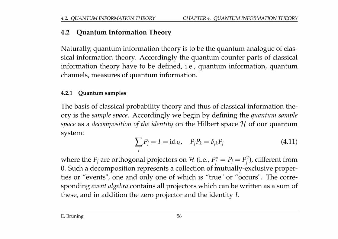
The basis of classical probability theory and thus of classical information the-ory is the sample space. Accordingly we begin by defining the quantum samplespace as a decomposition of the identity on the Hilbert space H of our quantumsystem:
∑j
Pj = I = idH, PjPk = δjkPj (4.11)
where the Pj are orthogonal projectors on H (i.e., P∗j = Pj = P2j ), different from
0. Such a decomposition represents a collection of mutually-exclusive proper-ties or “events", one and only one of which is “true" or “occurs". The corre-sponding event algebra contains all projectors which can be written as a sum ofthese, and in addition the zero projector and the identity I.
E. Brüning 56
CHAPTER 4. QUANTUM INFORMATION THEORY 4.2. QUANTUM INFORMATION THEORY
To such a quantum sample{
Pj}
one assigns probabilities{
pj}
. Typicallythese probabilities are generated through the use of the Born rule, see (2.11)and (2.12). Recall that the probability that a quantum observable has a partic-ular value is equal to the probability assigned to the projector onto the eigen-space of this eigen-value. Thus this projector must be part of some decompo-sition of the identity to which one has managed to assign probabilities. This isoften referred to as the probability that this observable will have this particularvalue “if measured".
4.2.2 Compatible and incompatible quantum samples
Two quantum samples{
Pj}
and {Qk} are compatible iff for every j,k
PjQk = QkPj ,
otherwise they are incompatible.The commutativity of the projection operators from one quantum sample or
two compatible quantum samples implies that all results of classical (Shannon)information theory carry over to the quantum domain, as expected.
Incompatible quantum samples must not be combined.
E. Brüning 57
4.2. QUANTUM INFORMATION THEORY CHAPTER 4. QUANTUM INFORMATION THEORY
4.2.3 Mutually-unbiased quantum samples
Two distinct quantum samples for a single qubit are always incompatible (thinkof the eigen-projections onto the eigen-spaces of the spin matrices σz and σx).But the degree of incompatibility may differ. The following definition ex-presses this in quantitative terms.
Observe that given an orthonormal basis{∣∣ej
⟩}of a Hilbert space H of
dimension m the family{[ej]}
of orthogonal projectors onto the subspacesspanned by the ej form a decomposition of the identity and thus a quantumsample.
Two orthonormal bases{∣∣ej
⟩}and
{∣∣ej⟩}
of H are called mutually unbiasediff for every j and every k
|⟨ej∣∣ ek⟩| = 1√
m, or Tr([ej][ek]) =
1m
. (4.12)
4.2.4 Quantum channels
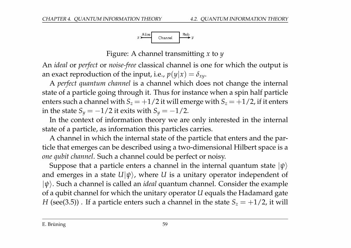
Recall that a classical channel (see figure below) is characterized by the condi-tional probability p(y|x) that a y emerges when a message x has been put intothe channel.
E. Brüning 58
CHAPTER 4. QUANTUM INFORMATION THEORY 4.2. QUANTUM INFORMATION THEORY
Figure: A channel transmitting x to y
An ideal or perfect or noise-free classical channel is one for which the output isan exact reproduction of the input, i.e., p(y|x) = δxy.
A perfect quantum channel is a channel which does not change the internalstate of a particle going through it. Thus for instance when a spin half particleenters such a channel with Sz =+1/2 it will emerge with Sz =+1/2, if it entersin the state Sy = −1/2 it exits with Sy = −1/2.
In the context of information theory we are only interested in the internalstate of a particle, as information this particles carries.
A channel in which the internal state of the particle that enters and the par-ticle that emerges can be described using a two-dimensional Hilbert space is aone qubit channel. Such a channel could be perfect or noisy.
Suppose that a particle enters a channel in the internal quantum state |ψ〉and emerges in a state U|ψ〉, where U is a unitary operator independent of|ψ〉. Such a channel is called an ideal quantum channel. Consider the exampleof a qubit channel for which the unitary operator U equals the Hadamard gateH (see(3.5)) . If a particle enters such a channel in the state Sz = +1/2, it will
E. Brüning 59
4.2. QUANTUM INFORMATION THEORY CHAPTER 4. QUANTUM INFORMATION THEORY
emerge in the state Sz =+1/2; if it enters in the state Sy =−1/2, it will emergein the state Sy = +1/2.
A quantum channel which transmits one type of quantum information, i.e.,one quantum sample corresponding to a particular orthonormal basis of thestate space, whereas all mutually unbiased quantum samples are turned intopure noise (that is no information is transmitted), is a perfect classical channelor perfectly decohering channel. If a quantum channel transmits all types ofquantum information perfectly, it is a perfect quantum channel.
Remark 4.2.1 One can show: If a quantum channel perfectly transmits two mutuallyunbiased quantum samples then it perfectly transmits all other quantum samples aswell.
4.2.5 von Neumann entropy
The counterpart of Shannon’s entropy (4.1) has to provide a measure whichquantifies “missing information" for any specific quantum sample. This canbe done as follows: Given a quantum sample (4.11) assign a probability dis-tribution p = (p1, p2, . . .) to it and calculate the Shannon entropy (4.1) for thisdistribution.
E. Brüning 60
CHAPTER 4. QUANTUM INFORMATION THEORY 4.2. QUANTUM INFORMATION THEORY
A very useful entropy measure which is independent of the quantum infor-mation type is the von Neumann entropy which is defined for general densitymatrices ρ by
S(ρ) = −Tr(ρ logρ) (4.13)
using spectral calculus (2.5). Since every density matrix ρ has the spectralrepresentation
ρ = ∑j
ρj[ej]
with eigen-values ρj > 0 and eigen-vectors ej one easily finds
S(ρ) = −∑j
ρj logρj, ρ = ∑j
ρj[ej] . (4.14)
Note the basic properties of the von Neumann entropy:
• S(ρ) ≥ 0 for every density matrix ρ and S(ρ) = 0 iff ρ is pure, i.e., of theform ρ = |ψ〉〈ψ| for a unit vector |ψ〉.
• For any invertible matrix U and any density matrix ρ one has S(UρU−1) =S(ρ), i.e., the von Neumann entropy is invariant under similarity transfor-mations.
E. Brüning 61
4.2. QUANTUM INFORMATION THEORY CHAPTER 4. QUANTUM INFORMATION THEORY
Often a density matrix ρ is considered a “pre-probability" and one can showthat the von Neumann entropy S(ρ) represents the minimum missing informa-tion associated with a pre-probability ρ.
E. Brüning 62
Chapter 5
Dense Coding, no Cloning and Teleportation
5.1 Fully entangled states and local unitaries
Recall that we mentioned earlier that entanglement is peculiar to quantummechanics and in quantum information theory entanglement is used as an im-portant resource. The first two cases we discuss are dense coding and telepor-tation. Thus we collect here some basic facts about a special class of entangledstates.
Suppose that Ha and Hb are two Hilbert spaces of dimension d. Recall that
63
5.1. FULLY ENTANGLED STATES CHAPTER 5. TELEPORTATION
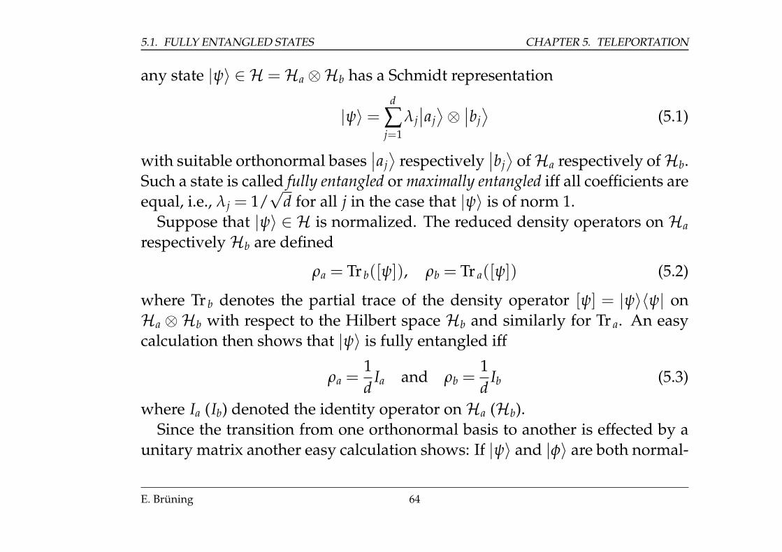
any state |ψ〉 ∈ H =Ha ⊗Hb has a Schmidt representation
|ψ〉 =d
∑j=1
λj∣∣aj⟩⊗∣∣bj⟩
(5.1)
with suitable orthonormal bases∣∣aj⟩
respectively∣∣bj⟩
ofHa respectively ofHb.Such a state is called fully entangled or maximally entangled iff all coefficients areequal, i.e., λj = 1/
√d for all j in the case that |ψ〉 is of norm 1.
Suppose that |ψ〉 ∈ H is normalized. The reduced density operators on Ha
respectivelyHb are defined
ρa = Tr b([ψ]), ρb = Tr a([ψ]) (5.2)
where Tr b denotes the partial trace of the density operator [ψ] = |ψ〉〈ψ| onHa ⊗Hb with respect to the Hilbert space Hb and similarly for Tr a. An easycalculation then shows that |ψ〉 is fully entangled iff
ρa =1d
Ia and ρb =1d
Ib (5.3)
where Ia (Ib) denoted the identity operator onHa (Hb).Since the transition from one orthonormal basis to another is effected by a
unitary matrix another easy calculation shows: If |ψ〉 and |φ〉 are both normal-
E. Brüning 64
CHAPTER 5. TELEPORTATION 5.1. FULLY ENTANGLED STATES
ized fully entangled states onHa⊗Hb there a unitary operators Ua onHa andUb onHb such that
|φ〉 = (Ua ⊗Ub)|ψ〉 . (5.4)
Since the subsystem A with the Hilbert space Ha and the subsystem B withthe Hilbert space Hb are often located in two separate laboratories one refersto the unitary operators Ua and Ub in (5.4) as local unitaries. And we can sayfor instance that a local operation in A can change a fully entangled state |ψ〉also in the distant location B!
For two qubits one has d = 2 and the states∣∣φ+⟩= |B0〉 = (|00〉+ |11〉)/
√2∣∣ψ+
⟩= |B1〉 = (|01〉+ |10〉)/
√2∣∣φ−⟩ = |B2〉 = (|00〉 − |11〉)/√
2∣∣ψ−⟩ = |B3〉 = (|01〉 − |10〉)/√
2
(5.5)
are fully entangled and are easily seen to be an orthonormal basis of H =C2⊗C2. These states are called Bell states .
Recall the action of the Pauli gates X and Z introduced in (3.6) and (3.7):
X : |0〉 −→ |1〉 , |1〉 −→ |0〉; Z : |0〉 −→ |0〉 , |1〉 −→ −|1〉 .
E. Brüning 65
5.2. DENSE CODING CHAPTER 5. TELEPORTATION
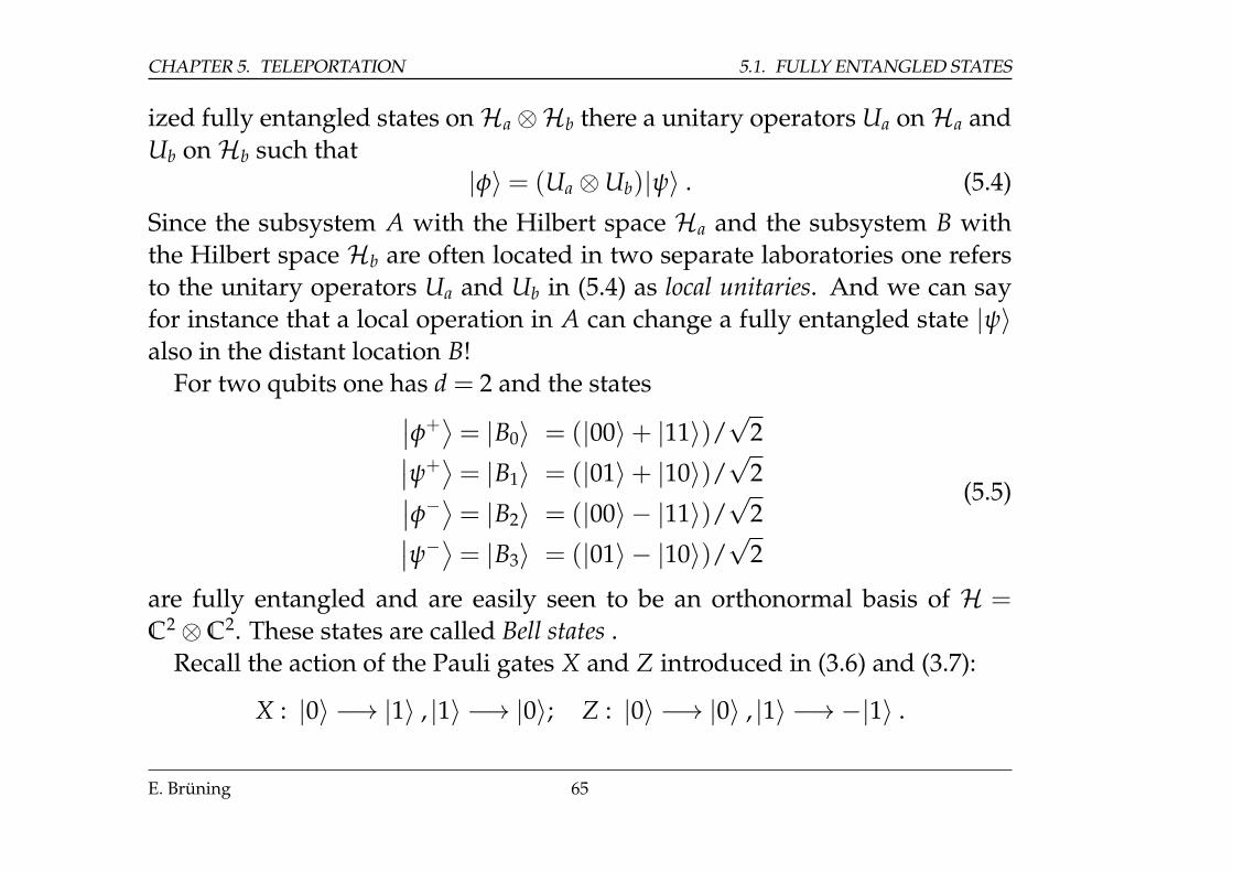
Now a straight forward calculation shows that the Bell states B1, B2, B3 can beobtained from the Bell state B0 by applying local unitaries:
|B1〉 = (X⊗ Ib)|B0〉|B2〉 = (Z⊗ Ib)|B0〉|B3〉 = (ZX⊗ Ib)|B0〉
(5.6)
5.2 Dense Coding
Dense coding (or often also called super dense coding) and teleportation aretwo processes which can be considered as the starting point of modern quan-tum information theory. Both demonstrated completely new features of quan-tum information as opposed to classical information and both are based on theuse of (fully) entangled states. The original papers 1 and 7 provided explicitexamples using qubits. Later many extensions of their schemes were found.An early systematic approach is proposed in 16. There it is shown in particularthat each of the published teleportation schemes also works as a dense codingscheme, and conversely (for tight schemes): Sender (Alice) and receiver (Bob)merely have to swap the equipment they use.
E. Brüning 66
CHAPTER 5. TELEPORTATION 5.2. DENSE CODING
We are going to explain the basic ideas for dense coding and teleportationonly for the simplest cases of qubits.
The essence of dense coding is: Suppose A and B have a quantum channelover which A can send qubits to B. One way to send her message is to encode0 as |0〉 and 1 as |1〉.
If A and B share a Bell state, then A can send two classical bits of informationusing only one qubit.
The details are as follows: Suppose A and B share the Bell state |φ+〉, see(5.5). Depending on the message Alice wants to send, she applies a suitablegate to her qubit and then sends it to Bob. If Alice wants to send
00011011
she applies
I2⊗ I2
Z⊗ I2
X⊗ I2
XZ⊗ I2
to |φ+〉 and gets
|φ+〉|φ−〉|ψ+〉|ψ−〉
where we used (5.6). After receiving the message from Alice, Bob has one ofthe four mutually orthogonal Bell states. When he applies a measurement hecan distinguish between them with certainty and thus can determine Alice’smessage.
E. Brüning 67
5.3. TELEPORTATION CHAPTER 5. TELEPORTATION
Note that Alice used two qubits in total so send two classical bits, since Aliceand Bob started with a shared Bell state. However, the first qubit, i.e., Bob’shalf of the Bell state, could have been sent well before Alice decided whatmessage she wanted to send. Only after she had decided on her message, shesent the second qubit.
And one can show that one cannot do better. Two qubits are necessary tosend two classical bits. Dense coding allows half the qubits to be sent beforethe message has been chosen.
5.3 Teleportation
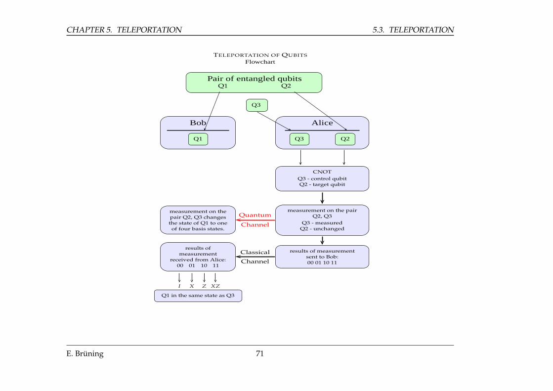
In the process of quantum teleportation or entanglement assisted teleporta-tion the state of a qubit is replaced by that of another. The state is “transmitted"by setting up an entangled state-space of three qubits and then removing twoqubits from the entanglement (via measurement). Since the information ofthe source qubit is preserved by these measurements that “information" (i.e.state) ends up in the final third, destination qubit. This occurs without thesource and destination qubit ever directly interacting. The interaction occursvia entanglement.
E. Brüning 68
CHAPTER 5. TELEPORTATION 5.3. TELEPORTATION
It is unrelated to the popular science fiction term of teleportation.The idea of teleporting qubits from one location A to a distant location B
was first suggested in 1993 in the seminal paper (7). Since then various exten-sions and generalizations (using photons or atoms) have been suggested, alsoexperimentally.
Distances of more than 100 km have been used in quantum teleportationexperiments.
The established protocol for teleportation of qubits between two distant lo-cations A and B reads:
1. An EPR pair (i.e., two entangled qubits in one of the Bell states, usually|φ+〉) is generated, and one qubit is send to location A, the other to locationB.
2. At A there are two qubits, one to be teleported, the other the qubit from theEPR pair. A Bell measurement of these two qubits is performed yieldingtwo classical bits and destroying these qubits in the process.
3. The two bits are sent from location A to B, using a classical channel, forinstance a telephone line.
E. Brüning 69
5.3. TELEPORTATION CHAPTER 5. TELEPORTATION
4. The qubit at B from the EPR pair is sent through a suitable quantum gate(determined by the two bits received from A) to produce a qubit which isidentical to the one to be teleported.
E. Brüning 70
CHAPTER 5. TELEPORTATION 5.3. TELEPORTATION
TELEPORTATION OF QUBITS
Flowchart
Pair of entangled qubitsQ1 Q2
Q3
Bob
Q1
Alice
Q3 Q2
CNOT
Q3 - control qubitQ2 - target qubit
measurement on the pairQ2, Q3
Q3 - measuredQ2 - unchanged
measurement on thepair Q2, Q3 changesthe state of Q1 to oneof four basis states.
results ofmeasurement
received from Alice:00 01 10 11
results of measurementsent to Bob:00 01 10 11
Quantum
Channel
Classical
Channel
XZZXI
Q1 in the same state as Q3
E. Brüning 71
5.3. TELEPORTATION CHAPTER 5. TELEPORTATION
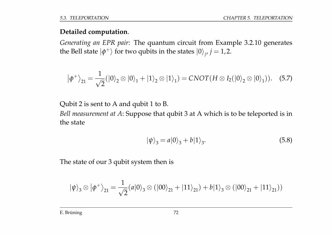
Detailed computation.
Generating an EPR pair: The quantum circuit from Example 3.2.10 generatesthe Bell state |φ+〉 for two qubits in the states |0〉j, j = 1,2.
∣∣φ+⟩
21 =1√2(|0〉2⊗ |0〉1 + |1〉2⊗ |1〉1) = CNOT(H ⊗ I2(|0〉2⊗ |0〉1)). (5.7)
Qubit 2 is sent to A and qubit 1 to B.Bell measurement at A: Suppose that qubit 3 at A which is to be teleported is inthe state
|ψ〉3 = a|0〉3 + b|1〉3. (5.8)
The state of our 3 qubit system then is
|ψ〉3⊗∣∣φ+⟩
21 =1√2(a|0〉3⊗ (|00〉21 + |11〉21) + b|1〉3⊗ (|00〉21 + |11〉21))
E. Brüning 72
CHAPTER 5. TELEPORTATION 5.3. TELEPORTATION
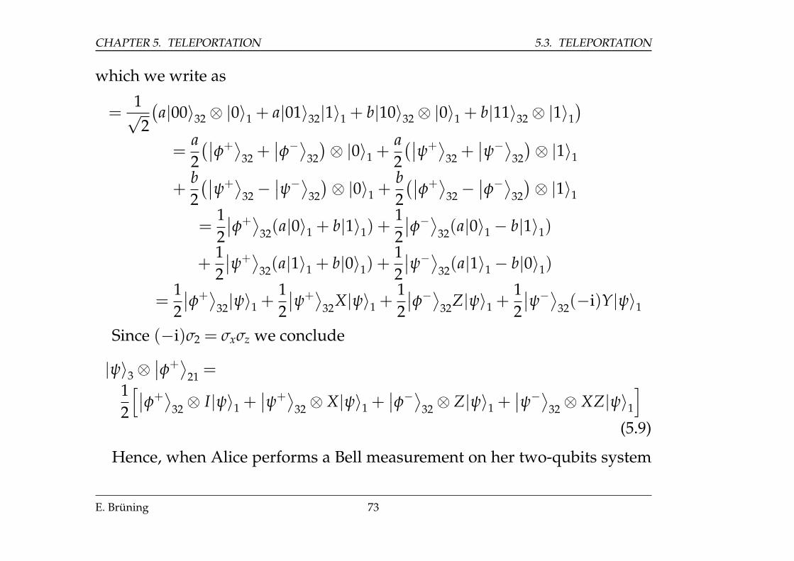
which we write as
=1√2
(a|00〉32⊗ |0〉1 + a|01〉32|1〉1 + b|10〉32⊗ |0〉1 + b|11〉32⊗ |1〉1
)=
a2(∣∣φ+
⟩32 +
∣∣φ−⟩32
)⊗ |0〉1 +
a2(∣∣ψ+
⟩32 +
∣∣ψ−⟩32
)⊗ |1〉1
+b2(∣∣ψ+
⟩32−
∣∣ψ−⟩32
)⊗ |0〉1 +
b2(∣∣φ+
⟩32−
∣∣φ−⟩32
)⊗ |1〉1
=12
∣∣φ+⟩
32(a|0〉1 + b|1〉1) +12
∣∣φ−⟩32(a|0〉1− b|1〉1)
+12
∣∣ψ+⟩
32(a|1〉1 + b|0〉1) +12
∣∣ψ−⟩32(a|1〉1− b|0〉1)
=12
∣∣φ+⟩
32|ψ〉1 +12
∣∣ψ+⟩
32X|ψ〉1 +12
∣∣φ−⟩32Z|ψ〉1 +12
∣∣ψ−⟩32(−i)Y|ψ〉1
Since (−i)σ2 = σxσz we conclude
|ψ〉3⊗∣∣φ+⟩
21 =
12
[∣∣φ+⟩
32⊗ I|ψ〉1 +∣∣ψ+
⟩32⊗ X|ψ〉1 +
∣∣φ−⟩32⊗ Z|ψ〉1 +∣∣ψ−⟩32⊗ XZ|ψ〉1
](5.9)
Hence, when Alice performs a Bell measurement on her two-qubits system
E. Brüning 73
5.3. TELEPORTATION CHAPTER 5. TELEPORTATION
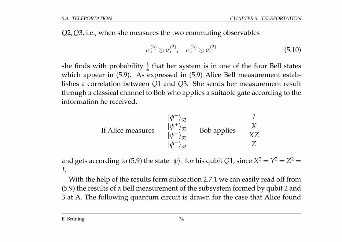
Q2, Q3, i.e., when she measures the two commuting observables
σ(3)x ⊗ σ
(2)x , σ
(3)z ⊗ σ
(2)z (5.10)
she finds with probability 14 that her system is in one of the four Bell states
which appear in (5.9). As expressed in (5.9) Alice Bell measurement estab-lishes a correlation between Q1 and Q3. She sends her measurement resultthrough a classical channel to Bob who applies a suitable gate according to theinformation he received.
If Alice measures
|φ+〉32|ψ+〉32|ψ−〉32|φ−〉32
Bob applies
IX
XZZ
and gets according to (5.9) the state |ψ〉1 for his qubit Q1, since X2 = Y2 = Z2 =I.
With the help of the results form subsection 2.7.1 we can easily read off from(5.9) the results of a Bell measurement of the subsystem formed by qubit 2 and3 at A. The following quantum circuit is drawn for the case that Alice found
E. Brüning 74
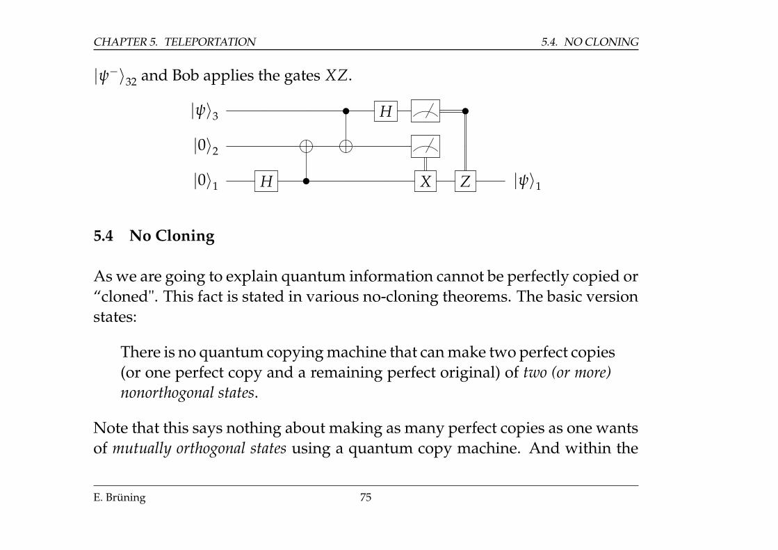
CHAPTER 5. TELEPORTATION 5.4. NO CLONING
|ψ−〉32 and Bob applies the gates XZ.
|ψ〉3 • H •
|0〉2
|0〉1 H • X Z |ψ〉1
5.4 No Cloning
As we are going to explain quantum information cannot be perfectly copied or“cloned". This fact is stated in various no-cloning theorems. The basic versionstates:
There is no quantum copying machine that can make two perfect copies(or one perfect copy and a remaining perfect original) of two (or more)nonorthogonal states.
Note that this says nothing about making as many perfect copies as one wantsof mutually orthogonal states using a quantum copy machine. And within the
E. Brüning 75
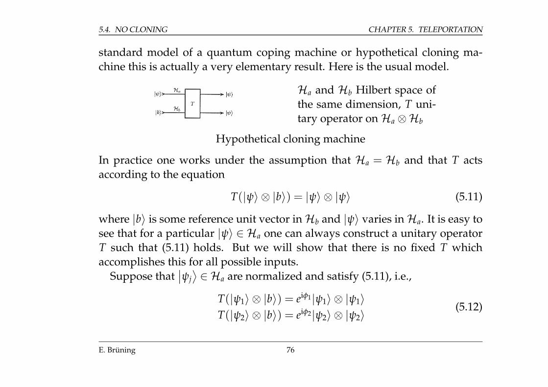
5.4. NO CLONING CHAPTER 5. TELEPORTATION
standard model of a quantum coping machine or hypothetical cloning ma-chine this is actually a very elementary result. Here is the usual model.
Ha and Hb Hilbert space ofthe same dimension, T uni-tary operator onHa ⊗Hb
Hypothetical cloning machine
In practice one works under the assumption that Ha = Hb and that T actsaccording to the equation
T(|ψ〉 ⊗ |b〉) = |ψ〉 ⊗ |ψ〉 (5.11)
where |b〉 is some reference unit vector inHb and |ψ〉 varies inHa. It is easy tosee that for a particular |ψ〉 ∈ Ha one can always construct a unitary operatorT such that (5.11) holds. But we will show that there is no fixed T whichaccomplishes this for all possible inputs.
Suppose that∣∣ψj⟩∈ Ha are normalized and satisfy (5.11), i.e.,
T(|ψ1〉 ⊗ |b〉) = eiφ1|ψ1〉 ⊗ |ψ1〉T(|ψ2〉 ⊗ |b〉) = eiφ2|ψ2〉 ⊗ |ψ2〉
(5.12)
E. Brüning 76
CHAPTER 5. TELEPORTATION 5.4. NO CLONING
where φj are some phases. Taking the inner product of these two identitiesgives, since T is unitary,
〈ψ1| ψ2〉 〈b| b〉 = ei(φ2−φ1) 〈ψ1| ψ2〉2
and thus| 〈ψ1| ψ2〉 | = | 〈ψ1| ψ2〉 |2 .
The only solutions to the last equation are | 〈ψ1| ψ2〉 | = 0 or | 〈ψ1| ψ2〉 | = 1. Inthe first case the two vectors are orthogonal and in the second case the twovectors are identical apart from a phase factor. This proves our claim.
Some further versions of no-cloning theorems are known; the above versiongives just the essential core.
E. Brüning 77
5.4. NO CLONING CHAPTER 5. TELEPORTATION
E. Brüning 78
Chapter 6
Quantum Cryptography
We recall here only very briefly a few basic facts from (classical) cryptography.Cryptography is about sending messages between two parties in such a waythat its contents cannot be understood by someone other than the indendedrecipient. The original message or plaintext is encrypted using an encryptionrule typically based on an encryption key to produce an unintelligible cybertext.The recipient then applies a decryption rule, using the same key to the cybertextin order to recover the original plaintext message.
The one-time pad (OTP) is a type of (classical) encryption which has beenproven to be impossible to crack if used correctly. Each bit or character fromthe plaintext is encrypted by modular addition with a bit or character from a
79
CHAPTER 6. QUANTUM CRYPTOGRAPHY
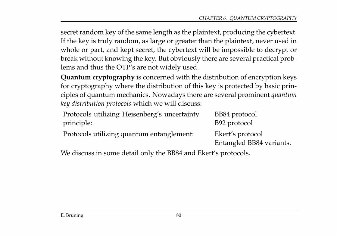
secret random key of the same length as the plaintext, producing the cybertext.If the key is truly random, as large or greater than the plaintext, never used inwhole or part, and kept secret, the cybertext will be impossible to decrypt orbreak without knowing the key. But obviously there are several practical prob-lems and thus the OTP’s are not widely used.Quantum cryptography is concerned with the distribution of encryption keysfor cryptography where the distribution of this key is protected by basic prin-ciples of quantum mechanics. Nowadays there are several prominent quantumkey distribution protocols which we will discuss:
Protocols utilizing Heisenberg’s uncertaintyprinciple:
BB84 protocolB92 protocol
Protocols utilizing quantum entanglement: Ekert’s protocolEntangled BB84 variants.
We discuss in some detail only the BB84 and Ekert’s protocols.
E. Brüning 80
CHAPTER 6. QUANTUM CRYPTOGRAPHY 6.1. THE BB84 SCHEME
6.1 The BB84 Scheme
C. Bennet and G. Brassard published in 1984 3 the first QKD (Quantum KeyDistribution) protocol. Today it is still one of the most prominent protocols.The basic idea of all HUP based protocols is as follows: Alice can transmita random secret key to Bob by sending a string of photons where the secretkey’s bits are encoded in the polarization of photons. Heisenberg’s Uncer-tainty Principle is used to guarantee that an eavesdropper cannot measurethese photons and transmit them to Bob without disturbing the state of thephotons in a detectable way and thus revealing her presence.
In the BB84 protocol the bits are encoded in the polarization states of a pho-ton. Usually one defines a binary 0 as a polarization of 0 degrees in the rec-tilinear basis or 45 degrees in the diagonal basis. And similarly a binary 1corresponds to 90 degrees in the rectilinear basis and 135 degrees in the diago-nal basis. Thus a bit can be represented by polarizing the photon with respectto one of these two bases.
E. Brüning 81
6.1. THE BB84 SCHEME CHAPTER 6. QUANTUM CRYPTOGRAPHY
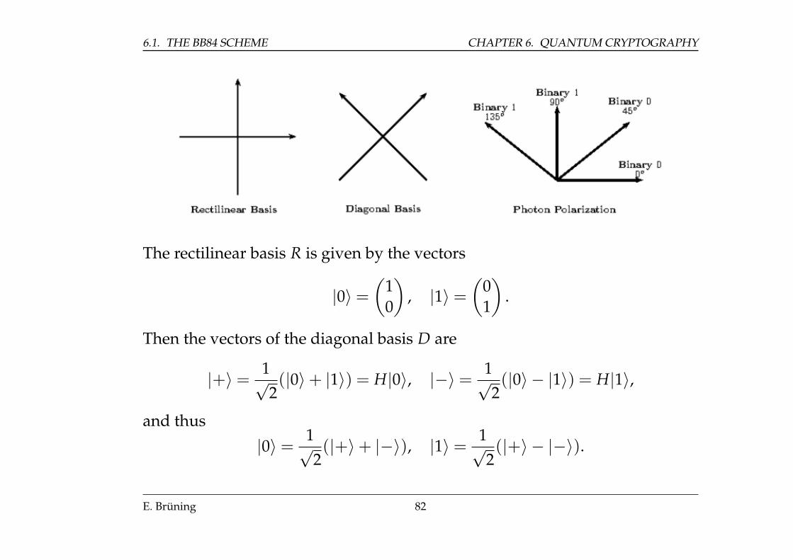
The rectilinear basis R is given by the vectors
|0〉 =(
10
), |1〉 =
(01
).
Then the vectors of the diagonal basis D are
|+〉 = 1√2(|0〉+ |1〉) = H|0〉, |−〉 = 1√
2(|0〉 − |1〉) = H|1〉,
and thus
|0〉 = 1√2(|+〉+ |−〉), |1〉 = 1√
2(|+〉 − |−〉).
E. Brüning 82
CHAPTER 6. QUANTUM CRYPTOGRAPHY 6.1. THE BB84 SCHEME
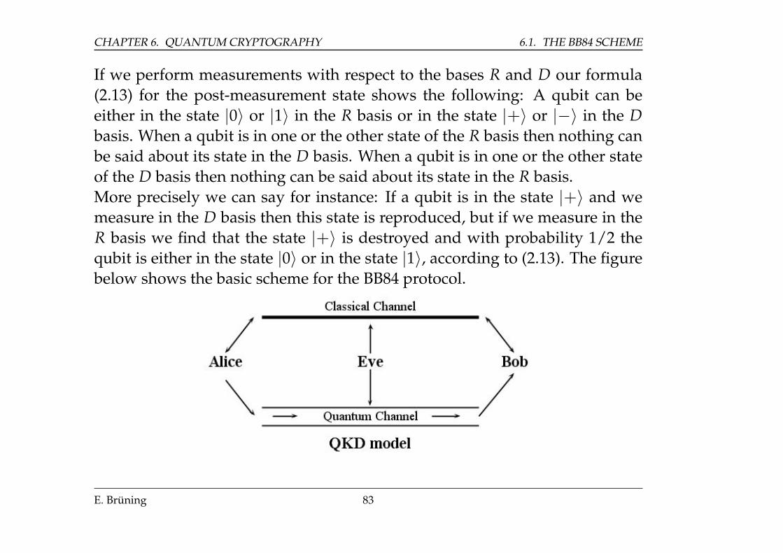
If we perform measurements with respect to the bases R and D our formula(2.13) for the post-measurement state shows the following: A qubit can beeither in the state |0〉 or |1〉 in the R basis or in the state |+〉 or |−〉 in the Dbasis. When a qubit is in one or the other state of the R basis then nothing canbe said about its state in the D basis. When a qubit is in one or the other stateof the D basis then nothing can be said about its state in the R basis.More precisely we can say for instance: If a qubit is in the state |+〉 and wemeasure in the D basis then this state is reproduced, but if we measure in theR basis we find that the state |+〉 is destroyed and with probability 1/2 thequbit is either in the state |0〉 or in the state |1〉, according to (2.13). The figurebelow shows the basic scheme for the BB84 protocol.
E. Brüning 83
6.1. THE BB84 SCHEME CHAPTER 6. QUANTUM CRYPTOGRAPHY
The various steps of the BB84 Quantum Key Distribution protocol are:
1. Alice and Bob decide (publicly) on an acceptable key length N, taking asensible error margin into account.
2. Secretly Alice chooses a random string of length 4N of data bits d1,d2, . . . ,d4N
and a random string of length 4N of letters a1, a2, . . . , a4N, aj ∈ {R, D}.
3. Bob too chooses secretly a random string of length 4N of letters b1,b2, . . . ,b4N,bj ∈ {R, D}.
4. Alice now does the following: For j ∈ {1,2, . . . ,4N} she prepares the jth
qubit in the state∣∣dj(aj)
⟩, i.e., the data value of the state is given by dj and
the basis is specified by aj. After this preparation Alice sends the jth qubitto Bob, through the quantum channel.
5. Bob receives the jth qubit and measures it in the basis bj and gets a classicalbit ej, for j ∈ {1,2, . . . ,4N}.
6. Alice and Bob exchange in public their basis label strings a1, a2, . . . , a4N
and b1,b2, . . . ,b4N. Now both know the indices at which a1, a2, . . . , a4N andb1,b2, . . . ,b4N agree, respectively disagree. They both discard those ele-
E. Brüning 84
CHAPTER 6. QUANTUM CRYPTOGRAPHY 6.1. THE BB84 SCHEME
ments where there is disagreement. This leaves a common string c1, c2, . . . , c 2N,cj ∈ {R, D}, which is typically of length about 2N.
7. Alice discards all elements of the string d1,d2, . . . ,d4N that do not corre-spond with elements of the string c1, c2, . . . , c 2N. This gives a string of bitsD1, D2, . . . , D 2N which is typically of length about 2N.
8. Bob discards the elements of the string e1, e2, . . . , e4N that do not correspondto elements of the string c1, c2, . . . , c 2N. This leave him with a string of bitsE1, E2, . . . , E 2N, again typically of length about 2N.
9. Note that cj, for each j ∈ {1,2, . . . , 2N}, is a basis name randomly cho-sen the same for the jth qubit by Alice for preparation and by Bob formeasurement. Thus the value Ej measured by Bob equals the value Dj
prepared and sent by Alice. Therefore the two binary strings are equal:D1, D2, . . . , D 2N = E1, E2, . . . , E 2N. This common string can thus serve as acandidate secret key for communication between Alice and Bob.
10. Alice and Bob choose publicly a randomly selected subsequence of c1, c2, . . . , c 2N,typically of length about N and exchange publicly the subsequences ofD1, D2, . . . , D 2N and E1, E2, . . . , E 2N that correspond to these values. They
E. Brüning 85
6.1. THE BB84 SCHEME CHAPTER 6. QUANTUM CRYPTOGRAPHY
should agree perfectly if there is no noise and/or eavesdropping.
11. If Eve has been eavesdropping, then about 25% of these values will disagree∗.In this case Alice and Bob have to start again.
12. If there was no eavesdropping the remaining subsequences of D1, D2, . . . , D 2N
and E1, E2, . . . , E 2N, each of typical length about N, constitute a common se-quence of bits K1,K2, . . . , K N which is secretly shared by Alice and Bob andcan serve as a secret key.
∗ Since Eve does not know the basis which has been assigned to each qubitshe is likely to guess the basis incorrectly 50% of the time, and thus when shemeasures, any time she guesses wrong she will destroy the original state of thequbit and the classical information she gets, i.e., the bits, will be wrong 50% ofthe time.
If one assumes a noiseless quantum channel and that there are no measure-ment errors, a disagreement in any of the bits which are compared wouldindicate the presence of an eavesdropper on the quantum channel. If Eve theeavesdropper would attempt to determine the key, she would have no choicebut to measure the photons sent by Alice before sending them to Bob. This isthe case since the no-cloning theorem assures that she cannot replicate a particle
E. Brüning 86
CHAPTER 6. QUANTUM CRYPTOGRAPHY 6.1. THE BB84 SCHEME
of unkown state. Since Eve will not know which bases Alice used to encode thebit until after Alice and Bob discuss their measurements, Eve has to guess. Ifshe measures on the incorrect basis, Heisenberg’s Uncertainty Principle ensuresthat the information encoded in the other basis is now lost. Thus when thephoton reaches Bob, his measurement will now be random and he will read abit incorrectly 50% of the time. Given that Eve will choose the measurementbasis incorrectly on average 50% of the time, 25% of Bob’s measured bits willdiffer from Alice’s. If Eve has eavesdropped on all the bits, then after n bitscomparisons by Alice and Bob, they will reduce the probability that Eve willnot be detected to (3
4)n. Hence the chance that an eavesdropper can be success-
ful will become negligible, if a sufficiently long sequence of bits are compared.
Here is an example for the BB84 protocol:
E. Brüning 87
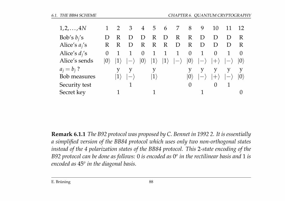
6.1. THE BB84 SCHEME CHAPTER 6. QUANTUM CRYPTOGRAPHY
1,2, . . . ,4N 1 2 3 4 5 6 7 8 9 10 11 12
Bob’s bj’s D R D D R D R R D D D RAlice’s aj’s R R D R R R D R D D D RAlice’s dj’s 0 1 1 0 1 1 1 0 1 0 1 0Alice’s sends |0〉 |1〉 |−〉 |0〉 |1〉 |1〉 |−〉 |0〉 |−〉 |+〉 |−〉 |0〉aj = bj ? y y y y y y y yBob measures |1〉 |−〉 |1〉 |0〉 |−〉 |+〉 |−〉 |0〉Security test 1 0 0 1Secret key 1 1 1 0
Remark 6.1.1 The B92 protocol was proposed by C. Bennet in 1992 2. It is essentiallya simplified version of the BB84 protocol which uses only two non-orthogonal statesinstead of the 4 polarization states of the BB84 protocol. This 2-state encoding of theB92 protocol can be done as follows: 0 is encoded as 0o in the rectilinear basis and 1 isencoded as 45o in the diagonal basis.
E. Brüning 88
CHAPTER 6. QUANTUM CRYPTOGRAPHY 6.2. EKERT’S PROTOCOL E91
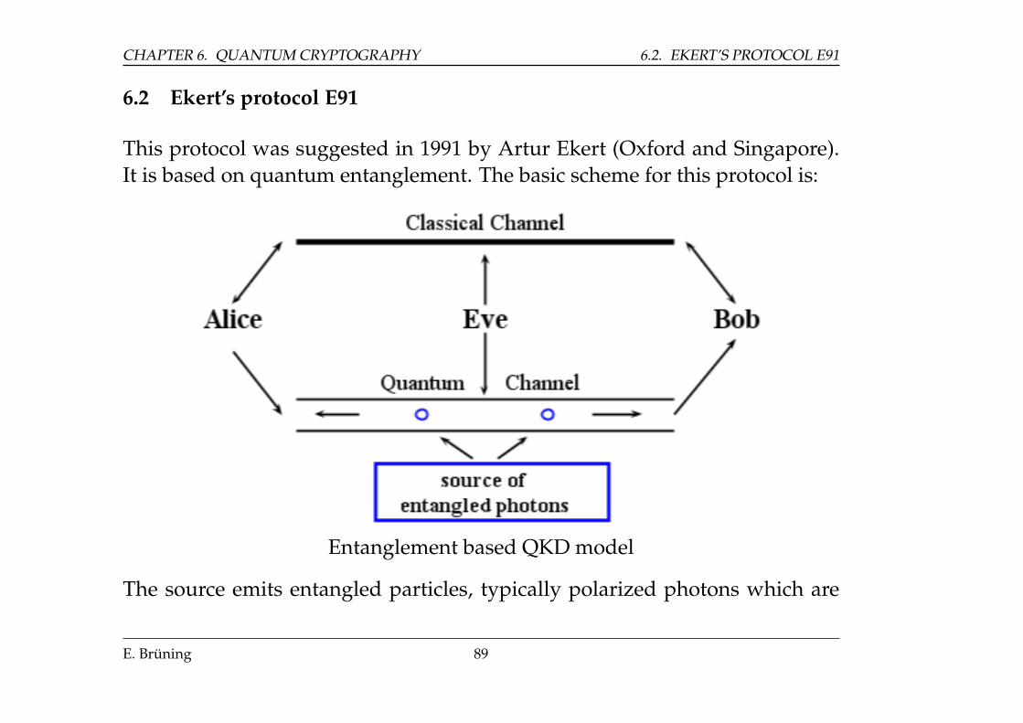
6.2 Ekert’s protocol E91
This protocol was suggested in 1991 by Artur Ekert (Oxford and Singapore).It is based on quantum entanglement. The basic scheme for this protocol is:
Entanglement based QKD model
The source emits entangled particles, typically polarized photons which are
E. Brüning 89
6.2. EKERT’S PROTOCOL E91 CHAPTER 6. QUANTUM CRYPTOGRAPHY
spatially separated. In detail the E91 quantum key distribution protocolreads:
0. Alice and Bob share 4N maximally entangled qubit pairs, i.e. Alice hasone qubit of each entangled pair and Bob has the other.
1. Alice and Bob publicly decide an an acceptable key length N taking a sen-sible error margin into account.
2. Alice secretly chooses a random string of length 4N of letters a1, a2, . . . , a4N,aj ∈ {R, D}.
3. Bob secretly chooses a random string of length 4N of letters b1,b2, . . . ,b4N,bj ∈ {R, D}.
4. For each j, 1≤ j ≤ 4N, Alice measures her qubit of the jth pair in the basisaj and gets a classical bit dj.
5. For each j, 1≤ j ≤ 4N, Bob measures his qubit of the jth pair in the basis bj
and gets a classical bit ej.
6. Alice and Bob exchange publicly their basic label strings a1, a2, . . . , a4N andb1,b2, . . . ,b4N. They both know now the indices at which a1, a2, . . . , a4N and
E. Brüning 90
CHAPTER 6. QUANTUM CRYPTOGRAPHY 6.2. EKERT’S PROTOCOL E91
b1,b2, . . . ,b4N agree and the indices at which a1, a2, . . . , a4N and b1,b2, . . . ,b4N
disagree. Alice and Bob discard the elements that disagree and they areleft with a common string (typically of length about 2N) c1, c2, . . . , c 2N.
7. Alice discards the elements of d1,d2, . . . ,d4N that do not correspond to c1, c2, . . . , c 2N
and gets a string of bits (typically of length about 2N) D1, D2, . . . , D 2N.
8. Bob discards the elements of e1, e2, . . . , e4N that do not correspond to c1, c2, . . . , c 2N
and gets a string of bits (typically of length about 2N) E1, E2, . . . , E 2N.
9. For each j ∈ {1,2, . . . , 2N}, cj is the name of a basis chosen the same byAlice and Bob for the jth pair of maximally entangled qubits , the value Ej
measured by Bob, equals the value Dj measured by Alice. Hence the twobinary strings are equal: D1, D2, . . . , D 2N = E1, E2, . . . , E 2N. Thus they canserve as a candidate secret key for communication between Alice and Bob.
10. Alice and Bob choose publicly a randomly selected subsequence of c1, c2, . . . , c 2N
(typically of length about N), and exchange in public the subsequences ofD1, D2, . . . , D 2N and E1, E2, . . . , E 2N that correspond to these values. Ideallythey should agree perfectly.
11. If Eve has been eavesdropping, or the environment has degraded the max-
E. Brüning 91
6.2. EKERT’S PROTOCOL E91 CHAPTER 6. QUANTUM CRYPTOGRAPHY
imal entanglement of the qubit pairs, a significant proportion of these val-ues will disagree. In this case, Alice and Bob must start again.
12. If not, the remaining subsequences of D1, D2, . . . , D 2N and E1, E2, . . . , E 2N
(each typically of length about N) constitute a common sequence of bitsK1,K2, . . . , K N, which is secretly shared by Alice and Bob, and thus canserve as a secret key.
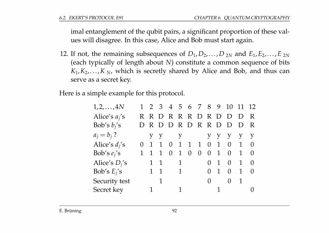
Here is a simple example for this protocol.
1,2, . . . ,4N 1 2 3 4 5 6 7 8 9 10 11 12Alice’s aj’s R R D R R R D R D D D RBob’s bj’s D R D D R D R R D D D Raj = bj ? y y y y y y y yAlice’s dj’s 0 1 1 0 1 1 1 0 1 0 1 0Bob’s ej’s 1 1 1 0 1 0 0 0 1 0 1 0Alice’s Dj’s 1 1 1 0 1 0 1 0Bob’s Ej’s 1 1 1 0 1 0 1 0Security test 1 0 0 1Secret key 1 1 1 0
E. Brüning 92
CHAPTER 6. QUANTUM CRYPTOGRAPHY 6.3. COMMERCIAL IMPLEMENTATIONS
6.3 Commercial implementations
Quantum key distribution is nowadays beyond the experimental phase. Be-side active research programs in various international companies (IBM, HP,Mitsubishi, NEC, NTT) there are three companies offering commercial quan-tum key distribution systems:
1. id Quantique (Geneva),
2. MagiQ Technologies (New York),
3. QuintessenceLabs (Australia).
Furthermore there are several quantum networks in operation.
1. DARPA Quantum Network: 10 nodes, running since 2004 in Massachusetts(USA); BBN Technologies, Harvard University, Boston University and Qine-tiQ.
2. SECOQC (Secure Communication based on Quantum Cryptography); theworld’s first computer network protected by quantum key distribution;implemented in 2008 in Vienna, using more than 200 km of standard fibreoptic cables.
E. Brüning 93
6.3. COMMERCIAL IMPLEMENTATIONS CHAPTER 6. QUANTUM CRYPTOGRAPHY
Special event: In 2004, the world’s first bank transfer using quantum keydistribution was carried out in Vienna, Austria.
3. SwissQuantum: started in 2007 by Id Quantique in Geneva, first for trans-mission of ballot results; from 2009 running reliably and stable for about2 years, confirming the viability of QKD as a commercial encryption tech-nology.
4. Tokyo QKD Network : The Tokyo QKD Network was inaugurated on thefirst day of the UQCC2010 conference. The network involves an inter-national collaboration between 7 partners; NEC, Mitsubishi Electric, NTTand NICT from Japan, and participation from Europe by Toshiba ResearchEurope Ltd. (UK), Id Quantique (Switzerland) and All Vienna (Austria)."All Vienna" is represented by researchers from the Austrian Institute ofTechnology (AIT), the Institute for Quantum Optics and Quantum Infor-mation (IQOQI) and the University of Vienna.
5. Durban Quantum Network: since 2009 running on the municipal standardfibre optic cables network;
special event in 2010: the connection of the football world cup soccer sta-dium to the municipal network was secured by QKD;
E. Brüning 94
CHAPTER 6. QUANTUM CRYPTOGRAPHY 6.3. COMMERCIAL IMPLEMENTATIONS
implemented by part of our group in Durban;
see http://quantum.ukzn.ac.za/
E. Brüning 95
6.3. COMMERCIAL IMPLEMENTATIONS CHAPTER 6. QUANTUM CRYPTOGRAPHY
E. Brüning 96
Chapter 7
Shor Factorization
On a classical computer the multiplication of large prime numbers can be im-plemented quite efficiently while the inverse function, i.e., finding the primefactors of a large number has not yet been solved by an efficient algorithm.Here an algorithm is called efficient if its execution time (the number of ele-mentary operations) is asymptotically polynomial in the length of its inputmeasured in bit. The classical quadratic sieve algorithm needs
O(e(
649 )1/3N1/3(ln N)2/3)
operations for factoring a binary number of N bits, i.e., this algorithm scalesexponentially with the input size. It seems to be the best algorithm for thisproblem.
97
CHAPTER 7. SHOR FACTORIZATION
Exercise: Using only pen and paper find the (prime) factors of
29083
This means that the multiplication of large prime numbers is essentially aone-way function which is the basis of the cryptographic algorithm developedin 1978 by Rivest, Shamir, and Adelman. This method became the most popu-lar public key system (RSA encryption).
It is believed that efficient prime factorization is impossible on a classicalcomputer. On a quantum computer however an efficient algorithm has beenproposed by P. Shor, inspired by work of D. Simon in 1994. This algorithmfinds the factors of a large composite number N, i.e., a number which can bewritten in the form
N = pq (7.1)
where the numbers p,q are assumed to be relatively prime which means thattheir greatest common divisor (gcd) is 1.
Here we will briefly explain the basic ideas for this factorization which takestime O((log N)3) and hence the integer factorization can be efficiently solvedon a quantum computer and is in the complexity class BQP (bounded errorquantum polynomial time).
E. Brüning 98
CHAPTER 7. SHOR FACTORIZATION
The realizability of Shor’s algorithm has first been shown at IBM in 2001where the number 15 was factored into 5× 3 using an NMR implementationof a quantum computer with 7 qubits. In 2012 a group in Bristol (UK) achievedthe factorization of 21. At present it is not yet possible to factor really largenumbers since only relatively small quantum computers can be build.
The factorization method of Shor has two main parts, a classical part basedon results from number theory and classical computation, and a quantum part.Under suitable restrictions the factorization problem is reduced in the classicalpart to that of a ’period finding problem’. For a solution of the period find-ing problem a suitable quantum computer is constructed which realizes thequantum Fourier transform through which the discrete spectrum of the periodfunction in question can be determined approximately. Some post-processingthen allows to calculate the period.
We begin by recalling some mathematical background, then proceed to ex-plain the reduction of the factorization problem to the period finding problemand in the main part present the core of Shor’s quantum algorithm.
E. Brüning 99
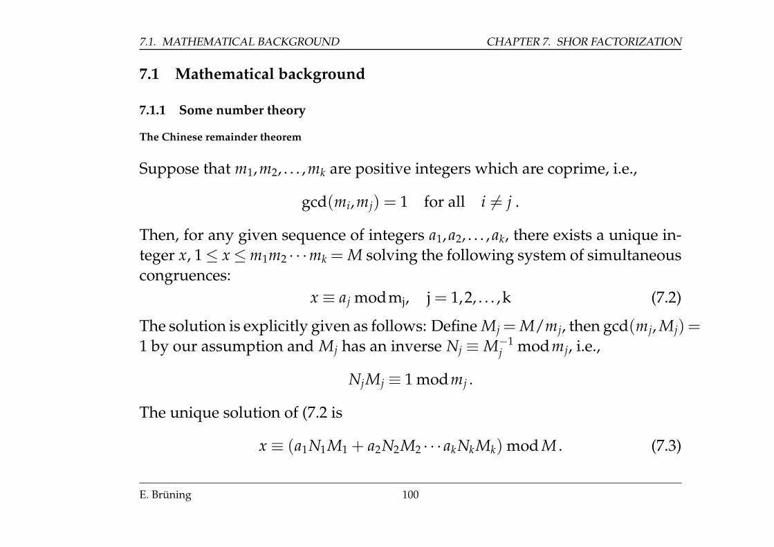
7.1. MATHEMATICAL BACKGROUND CHAPTER 7. SHOR FACTORIZATION
7.1 Mathematical background
7.1.1 Some number theory
The Chinese remainder theorem
Suppose that m1,m2, . . . ,mk are positive integers which are coprime, i.e.,
gcd(mi,mj) = 1 for all i 6= j .
Then, for any given sequence of integers a1, a2, . . . , ak, there exists a unique in-teger x, 1≤ x≤m1m2 · · ·mk = M solving the following system of simultaneouscongruences:
x ≡ aj modmj, j = 1,2, . . . ,k (7.2)
The solution is explicitly given as follows: Define Mj = M/mj, then gcd(mj, Mj) =1 by our assumption and Mj has an inverse Nj ≡ M−1
j modmj, i.e.,
NjMj ≡ 1 modmj .
The unique solution of (7.2 is
x ≡ (a1N1M1 + a2N2M2 · · · akNkMk) mod M . (7.3)
E. Brüning 100
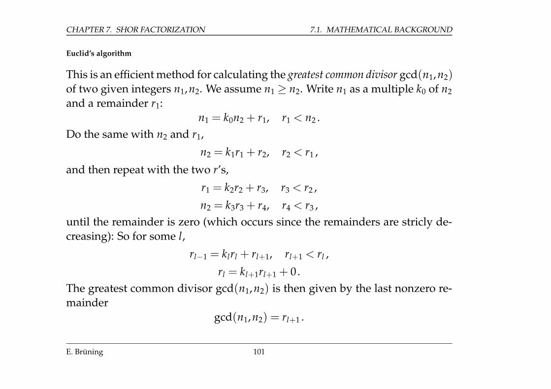
CHAPTER 7. SHOR FACTORIZATION 7.1. MATHEMATICAL BACKGROUND
Euclid’s algorithm
This is an efficient method for calculating the greatest common divisor gcd(n1,n2)of two given integers n1,n2. We assume n1 ≥ n2. Write n1 as a multiple k0 of n2
and a remainder r1:n1 = k0n2 + r1, r1 < n2 .
Do the same with n2 and r1,
n2 = k1r1 + r2, r2 < r1 ,
and then repeat with the two r’s,
r1 = k2r2 + r3, r3 < r2 ,
n2 = k3r3 + r4, r4 < r3 ,until the remainder is zero (which occurs since the remainders are stricly de-creasing): So for some l,
rl−1 = klrl + rl+1, rl+1 < rl ,
rl = kl+1rl+1 + 0.The greatest common divisor gcd(n1,n2) is then given by the last nonzero re-mainder
gcd(n1,n2) = rl+1 .
E. Brüning 101
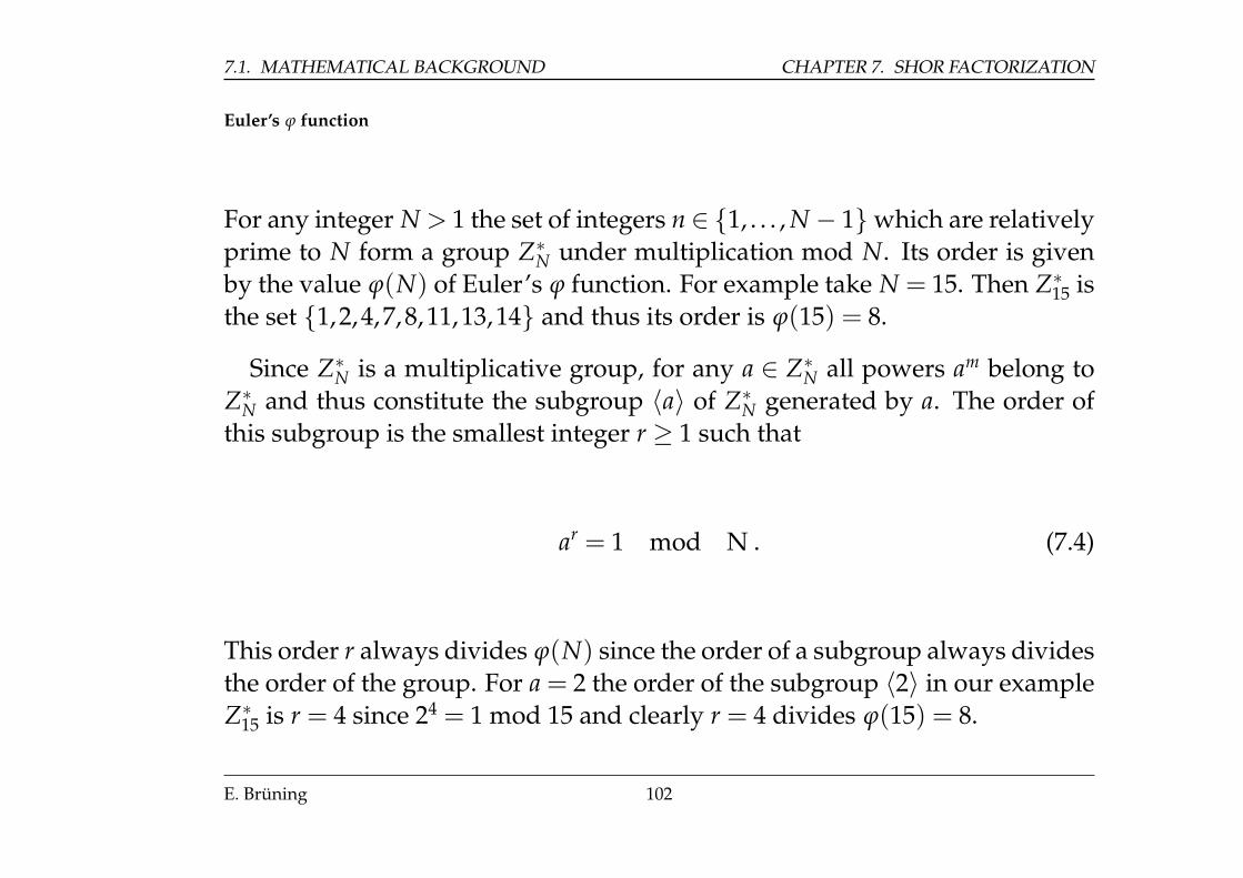
7.1. MATHEMATICAL BACKGROUND CHAPTER 7. SHOR FACTORIZATION
Euler’s ϕ function
For any integer N > 1 the set of integers n ∈ {1, . . . , N − 1}which are relativelyprime to N form a group Z∗N under multiplication mod N. Its order is givenby the value ϕ(N) of Euler’s ϕ function. For example take N = 15. Then Z∗15 isthe set {1,2,4,7,8,11,13,14} and thus its order is ϕ(15) = 8.
Since Z∗N is a multiplicative group, for any a ∈ Z∗N all powers am belong toZ∗N and thus constitute the subgroup 〈a〉 of Z∗N generated by a. The order ofthis subgroup is the smallest integer r ≥ 1 such that
ar = 1 mod N . (7.4)
This order r always divides ϕ(N) since the order of a subgroup always dividesthe order of the group. For a = 2 the order of the subgroup 〈2〉 in our exampleZ∗15 is r = 4 since 24 = 1 mod 15 and clearly r = 4 divides ϕ(15) = 8.
E. Brüning 102
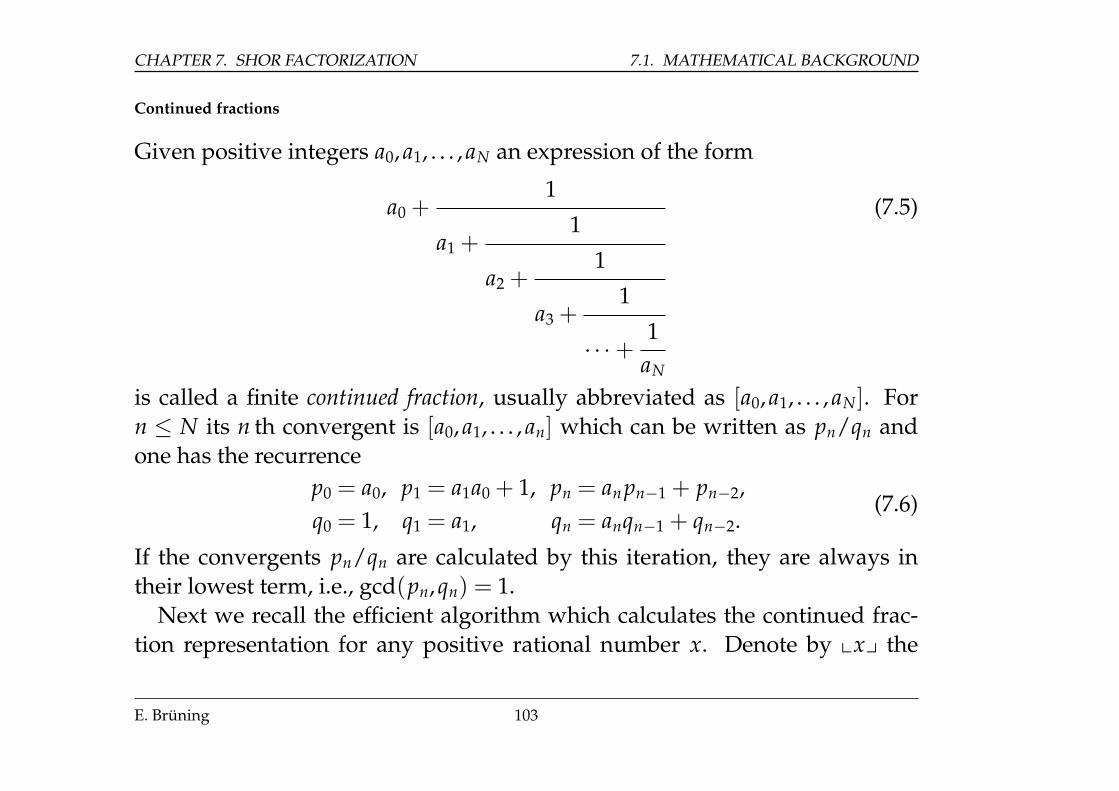
CHAPTER 7. SHOR FACTORIZATION 7.1. MATHEMATICAL BACKGROUND
Continued fractions
Given positive integers a0, a1, . . . , aN an expression of the form
a0 +1
a1 +1
a2 +1
a3 +1
· · ·+1
aN
(7.5)
is called a finite continued fraction, usually abbreviated as [a0, a1, . . . , aN]. Forn ≤ N its n th convergent is [a0, a1, . . . , an] which can be written as pn/qn andone has the recurrence
p0 = a0, p1 = a1a0 + 1, pn = anpn−1 + pn−2,q0 = 1, q1 = a1, qn = anqn−1 + qn−2.
(7.6)
If the convergents pn/qn are calculated by this iteration, they are always intheir lowest term, i.e., gcd(pn,qn) = 1.
Next we recall the efficient algorithm which calculates the continued frac-tion representation for any positive rational number x. Denote by xxy the
E. Brüning 103
7.1. MATHEMATICAL BACKGROUND CHAPTER 7. SHOR FACTORIZATION
greatest integer less than or equal to x. Then, with a0 = xxy, write x = a0 + ξ0
for some 0 ≤ ξ0 < 1. If ξ0 > 0, define a1 = x1/ξ0y and thus 1/ξ0 = a1 + ξ1 forsome 0 ≤ ξ1 < 1. If ξ1 > 0 define a2 = x1/ξ1y, etc. Since x is assumed to berational this process terminates and we get x = [a0, a1, . . . , an].
Eq. (7.5) shows that
[a0, a1, . . . , aN−1, aN] = [a0, a1, . . . , aN−1, aN − 1,1]
holds. Thus if we impose the condition aN > 1 the representation of x as acontinued fraction is unique.
We are going to use the following result.
Theorem 7.1.1 Suppose that p/q is a rational number satisfying∣∣pq− x∣∣ < 1
2q2 .
Then p/q is a convergent of the continued fraction of x.
7.1.2 Quantum Fourier transform
The quantum Fourier transform is the classical discrete Fourier transform act-ing on the vector of amplitudes of a quantum state. Recall that the classical
E. Brüning 104
CHAPTER 7. SHOR FACTORIZATION 7.1. MATHEMATICAL BACKGROUND
discrete Fourier transform sends a vector (x0, x1, . . . , xN−1) ∈ CN to the vector(y0,y1, . . . ,yN−1) ∈ CN with
yk =1√N
N−1
∑j=0
ω jkxj,
where ω denotes the canonical Nth primitive root of unity in the complexplane, i.e., ω = e
2πiN . Accordingly the quantum Fourier transform sends the
quantum state ∑N−1j=0 xj|j〉 to the quantum state ∑N−1
j=0 yj|j〉 where the yj’s aregiven by the same formula.
Naturally the quantum Fourier transform can be described as a unitary ma-trix acting on qubit states. The gate QFTn on n qubits is defined as the N × Nunitary matrix, N = 2n,
QFTn =( ω jk√
N
)0≤j,k≤N−1 =
1√N·
1 1 1 · · · 11 ω1 ω2 · · · ω(N−1)·1
1 ω2 ω4 · · · ω(N−1)·2... ... ... . . . ...1 ωN−1 ω2·(N−1) · · · ω(N−1)2
(7.7)
It is a simple calculation to show that this matrix is indeed unitary.
E. Brüning 105
7.1. MATHEMATICAL BACKGROUND CHAPTER 7. SHOR FACTORIZATION
For applications it is important that the quantum Fourier transform can beimplemented by a relatively simple quantum circuit which we describe now.
Consider an n qubit system. Its states can be represented in binary form
|x〉 = |x1, x2, . . . , xn〉 = |x1〉 ⊗ |x2〉 ⊗ · · · ⊗ |xn〉, xj ∈ {0,1}
where the xj are the binary digits in the representation x = ∑nj=1 xj2n−j. Intro-
duce the abbreviation [0.x1 · · · xn] for the binary fraction ∑nj=1 xj2−j and abbre-
viate
λj(x) = e2πi·[0.xj···xn].
This allows to realize the quantum Fourier transform in an simple way:
Proposition 7.1.2 The quantum Fourier transform on n qubits is given by the map
|x〉 −→ 1√N
n−1⊗j=0
(|0〉+ λn−j(x)|1〉
)(7.8)
E. Brüning 106
CHAPTER 7. SHOR FACTORIZATION 7.1. MATHEMATICAL BACKGROUND
The proof is a straight forward calculation.
√N · |x1, x2, . . . , xn〉 −→
N−1
∑k=0
e2πixk
N |k〉
= ∑k1∈{0,1}
· · · ∑kn∈{0,1}
e2πix∑n
j=1 kj2n−j
2n |k1, . . . ,kn〉
= ∑k1∈{0,1}
· · · ∑kn∈{0,1}
e2πix∑nj=1 kj2−j
|k1, . . . ,kn〉
= ∑k1∈{0,1}
· · · ∑kn∈{0,1}
n⊗j=1
e2πixkj2−j∣∣k j⟩
=n⊗
j=1
(∑
kj∈{0,1}e2πixkj2−j∣∣k j
⟩)=
n⊗j=1
(|0〉+ e2πix2−j|1〉) =n−1⊗j=0
(|0〉+ eπix2−j|1〉)
=n−1⊗j=0
(|0〉+ eπi[0.xn−j···xn]|1〉)
E. Brüning 107
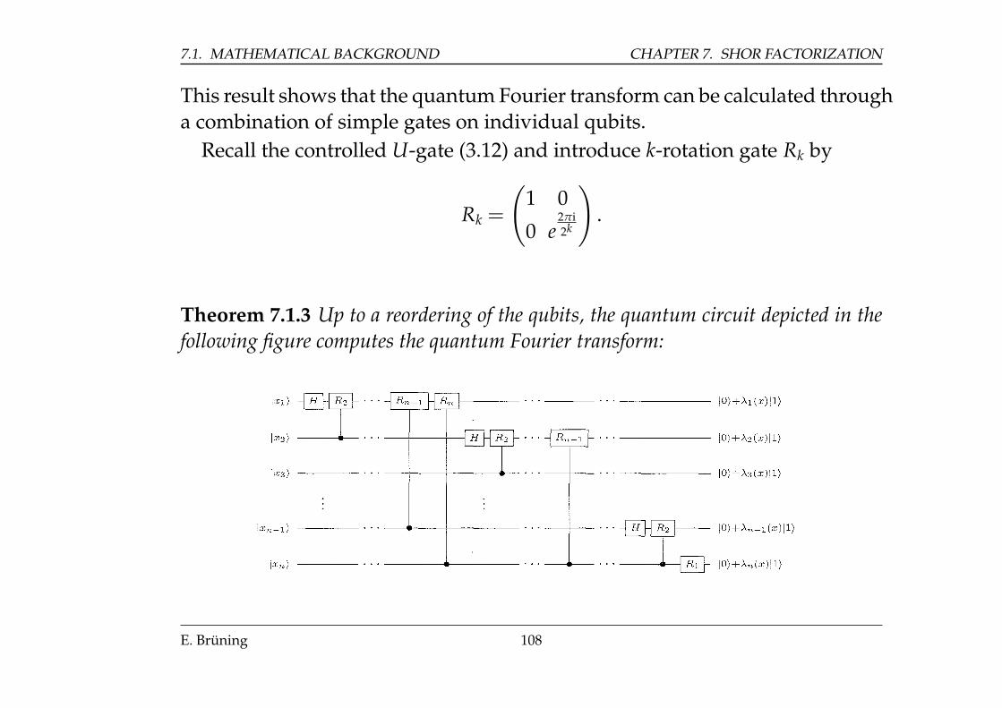
7.1. MATHEMATICAL BACKGROUND CHAPTER 7. SHOR FACTORIZATION
This result shows that the quantum Fourier transform can be calculated througha combination of simple gates on individual qubits.
Recall the controlled U-gate (3.12) and introduce k-rotation gate Rk by
Rk =
(1 0
0 e2πi2k
).
Theorem 7.1.3 Up to a reordering of the qubits, the quantum circuit depicted in thefollowing figure computes the quantum Fourier transform:
E. Brüning 108
CHAPTER 7. SHOR FACTORIZATION 7.2. REDUCTION TO PERIOD FINDING
7.2 Shor’s reduction of the factorization problem to order finding
Let N ∈N be given; consider the quadratic equation
x2 ≡ 1 modN. (7.9)
This equation always has the trivial solutions x ≡ 1 modN. If N is an oddprime number p, then these are the only solutions, since multiplication mod-ulo p has inverses and x2− 1≡ (x + 1)(x− 1) ≡ 0 mod p implies x− 1≡ 0 orx + 1≡ 0 mod p. For a composite number N there are however also non-trivialpairs of solutions x = ±a mod N as we show now: Assume that N is of theform N = n1n2 with gcd(n1,n2) = 1 and consider the following set of equiva-lences:
(a)
{x1 ≡ 1 modn1
x1 ≡ 1 modn2(a)
{x2 ≡ −1 modn1
x2 ≡ −1 modn2
(c)
{x3 ≡ 1 modn1
x3 ≡ −1 modn2(d)
{x4 ≡ −1 modn1
x4 ≡ 1 modn2(7.10)
In all four sets of equivalences xj ≡ 1 mod n1 and mod n2; each xj satisfiesEquation (7.9). By the Chinese remainder theorem each set has a unique so-lution mod N. From (a) and (b) we get the trivial solutions of Equation (7.9)
E. Brüning 109
7.2. REDUCTION TO PERIOD FINDING CHAPTER 7. SHOR FACTORIZATION
x1 ≡ 1 and x2 ≡ −1 mod N, while from (c) and (d) we get a non-trivial pairx3 ≡ a and x4 ≡ −a mod N of Equation (7.9). It follows that (a + 1)(a− 1) ≡ 0mod N and a± 1 are nonzero. Hence N divides (a + 1)(a− 1), but does notdivide a± 1, since a± 1≤ N + 1. Hence the greatest common divisor of N anda± 1 for a 6= ±1 is a nontrivial factor of N. And Euclid’s algorithm allows todetermine the greatest commen divisor of two given numbers efficiently.
How can we find a nontrivial solution x of Equation (7.9)? Choose a randomy < N. If y and N are coprime , let r be the order of y mod N. And this is theperiod of the function for y and N, i.e., for
FN(a) = ya modN. (7.11)
Thereforeyr = 1 modN. (7.12)
If r is an even number and if we set
x = yr/2, (7.13)
then we have x2 ≡ 1 mod N and thus x is a candidate for a nontrivial solutionof Equation (7.9).
Certainly this procedure may fail if we have chosen a y which has an oddorder r, or if r is even but yr/2 turns out to be a trivial solution of Equation (7.9).
E. Brüning 110
CHAPTER 7. SHOR FACTORIZATION 7.2. REDUCTION TO PERIOD FINDING
Fortunately the following result shows that the probability for this to happenis suitably small if y is chosen at random.
Theorem 7.2.1 Let N be an odd number with prime factorization
N = pm11 pm2
2 · · · pmkk . (7.14)
Choose a number y, 1≤ y ≤ N at random, satisfying gcd(y, N) = 1. If r is the orderof y mod N, then
Prob(r is even and yr/2 6≡ ±1modN) ≥ 1− 12k−1 . (7.15)
Note that in the case that N is even the factor 2 is easily detected and removed.
Remark 7.2.2 For the proof of the above theorem see 10. It can be extended to showthat
Prob(r is even and yr/2 6≡ ±1modN) ≥ 12
(7.16)
holds for all N which are not of the form pm or 2pm. In these cases the above proba-bility is zero. But pure prime powers pm are known to be efficiently recognizable by aclassical probabilistic algorithm.
One can also show that for a random selection of y, 1 ≤ y ≤ N, the probabilityof gcd(y, N) = 1 is greater than 1/log N. Thus, if we apply the above process to
E. Brüning 111
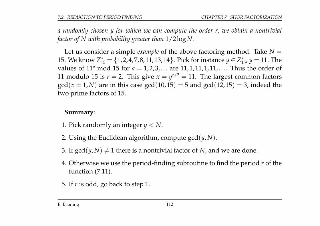
7.2. REDUCTION TO PERIOD FINDING CHAPTER 7. SHOR FACTORIZATION
a randomly chosen y for which we can compute the order r, we obtain a nontrivialfactor of N with probability greater than 1/2log N.
Let us consider a simple example of the above factoring method. Take N =15. We know Z∗15 = {1,2,4,7,8,11,13,14}. Pick for instance y ∈ Z∗15, y = 11. Thevalues of 11a mod 15 for a = 1,2,3, . . . are 11,1,11,1,11, . . .. Thus the order of11 modulo 15 is r = 2. This give x = yr/2 = 11. The largest common factorsgcd(x ± 1, N) are in this case gcd(10,15) = 5 and gcd(12,15) = 3, indeed thetwo prime factors of 15.
Summary:
1. Pick randomly an integer y < N.
2. Using the Euclidean algorithm, compute gcd(y, N).
3. If gcd(y, N) 6= 1 there is a nontrivial factor of N, and we are done.
4. Otherwise we use the period-finding subroutine to find the period r of thefunction (7.11).
5. If r is odd, go back to step 1.
E. Brüning 112
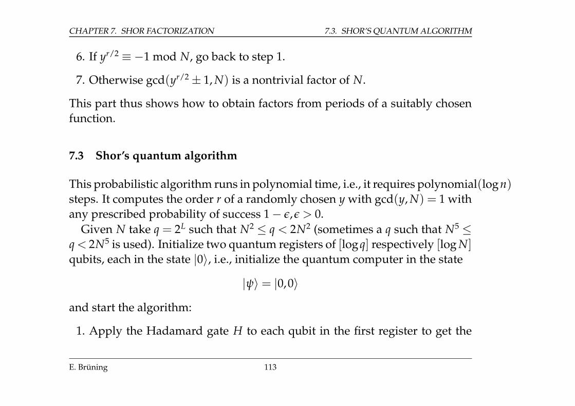
CHAPTER 7. SHOR FACTORIZATION 7.3. SHOR’S QUANTUM ALGORITHM
6. If yr/2 ≡ −1 mod N, go back to step 1.
7. Otherwise gcd(yr/2± 1, N) is a nontrivial factor of N.
This part thus shows how to obtain factors from periods of a suitably chosenfunction.
7.3 Shor’s quantum algorithm
This probabilistic algorithm runs in polynomial time, i.e., it requires polynomial(logn)steps. It computes the order r of a randomly chosen y with gcd(y, N) = 1 withany prescribed probability of success 1− ε,ε > 0.
Given N take q = 2L such that N2 ≤ q < 2N2 (sometimes a q such that N5 ≤q < 2N5 is used). Initialize two quantum registers of [logq] respectively [log N]qubits, each in the state |0〉, i.e., initialize the quantum computer in the state
|ψ〉 = |0,0〉
and start the algorithm:
1. Apply the Hadamard gate H to each qubit in the first register to get the
E. Brüning 113
7.3. SHOR’S QUANTUM ALGORITHM CHAPTER 7. SHOR FACTORIZATION
state1√
q
q−1
∑a=0|a〉|0〉.
2. Compute FN(a) = ya mod N in the second register, which gives the state
1√
q
q−1
∑a=0|a〉|ya modN〉.
3. Measure the second register. It can be in a base state |k〉 where k is somepower of x mod N. Denote by A the set of all a < q such that xa mod Nequals k and denote by M the number of elements in A. Then the post-measurement state is
|ψ〉 = 1√M
∑a∈A|a,k〉.
Note that A has the representation
A = {a0, a0 + r, a0 + 2r, . . . , a0 + (M− 1)r}with M ≈ q
r � 1. Thus the post-measurement state can be written as
|ψ〉 = 1√M
M−1
∑d=0|a0 + dr,k〉.
E. Brüning 114
CHAPTER 7. SHOR FACTORIZATION 7.3. SHOR’S QUANTUM ALGORITHM
4. Apply the quantum Fourier transform QFTq to the first register of thispost-measurement state to get the state
1√qM
q−1
∑c=0
M−1
∑d=0
e2πic(a0+dr)/q|c,k〉 =q−1
∑c=0
e2πica0/q√qM
M−1
∑d=0
ζd|c,k〉
where ζ = e2πicr/q.
5. Measure register 1. We observe register 1 to be in a particular state |c〉withprobability
Pr(c) =1
qM
∣∣∣M−1
∑d=0
ζd∣∣∣2 = 1
qM
∣∣∣1− ζM
1− ζ
∣∣∣2 = 1qM
sin2(πMcr/q)sin2(πcr/q)
. (7.17)
If crq is not very ‘close’ to an integer, then powers of ζ very nearly cancel
out (‘destructive interference’) and such states |c〉 are extremely unlikelyto be observed. In this case this probability is small.
However, if for some integer d one has
crq≈ d
E. Brüning 115
7.3. SHOR’S QUANTUM ALGORITHM CHAPTER 7. SHOR FACTORIZATION
then ζ ≈ 1 and therefore, using periodicity of sin2(θ + kπ) = sin2(θ) fork ∈Z
Pr(c) ≈ 1qM
M2 =Mq
is much larger. Hence the observed probability distribution is concen-trated around values of c for which
cq≈ d
rfor some integer d . (7.18)
6. For the observed value of c one uses a classical computer to find fractionsd/r very close to c/q, expecting that this will give the true order r of xmod N. For this one uses the method of continued fractions to computethe convergents dj/rj to c/q, see Theorem 7.1.1.
7. Here some more details of Step 6. According to (7.17) there are exactly rvalues of c mod q which satisfy
−r/2≤ rc mod q≤ r/2 (7.19)
and we wish to extract the value of r , given a value of c satisfying (7.19).
E. Brüning 116
CHAPTER 7. SHOR FACTORIZATION 7.3. SHOR’S QUANTUM ALGORITHM
Note that (7.19) is equivalent to∣∣ cq− c′
r∣∣ ≤ 1
q(7.20)
where c and q are known and r ≤ N, q ≥ N2.
Because of q ≤ N2, there is exactly one fraction c′/r with denominator atmost N in the range determined by (7.20). And this fraction may be foundby using the continued fraction expansion of c/q as one of its convergentsc′/q. Hence, if gcd(c′,r) = 1, we get the value of r.
Remark 7.3.1 The essential point of this period finding algorithm is the ability of aquantum computer to be in many states simultaneously (superposition of states). Thisallows to compute the period of a function F by evaluating its values simultaneouslyat all points.
As we know in quantum physics we get access to this information only throughmeasurement. But a measurement will give only one of all possible values and de-stroys all others. The no cloning theorem forbids to make suitable copies before themeasurement takes place. Therefore the superposition has been carefully transformedto another state that will return the correct answer with high probability. For thistransformation the quantum Fourier transformation has been used.
E. Brüning 117
7.3. SHOR’S QUANTUM ALGORITHM CHAPTER 7. SHOR FACTORIZATION
Remark 7.3.2 In order to implement the function (7.11) as a quantum transformone uses repeated squaring for the modular exponentiation transformation. This stepis actually more difficult to implement than the quantum Fourier transform and itrequires ancillary qubits and substantially more gates to implement. This results in aconsiderable slow down of the algorithm in concrete realizations.
E. Brüning 118
Chapter 8
Other important Topics
8.1 Deutsch: Universal Quantum Computer
8.2 Grover’s search algorithm for unsorted database
8.3 Quantum Error Correction
8.4 Quantum Complexity Theory
8.5 Continuous variable QKD
119
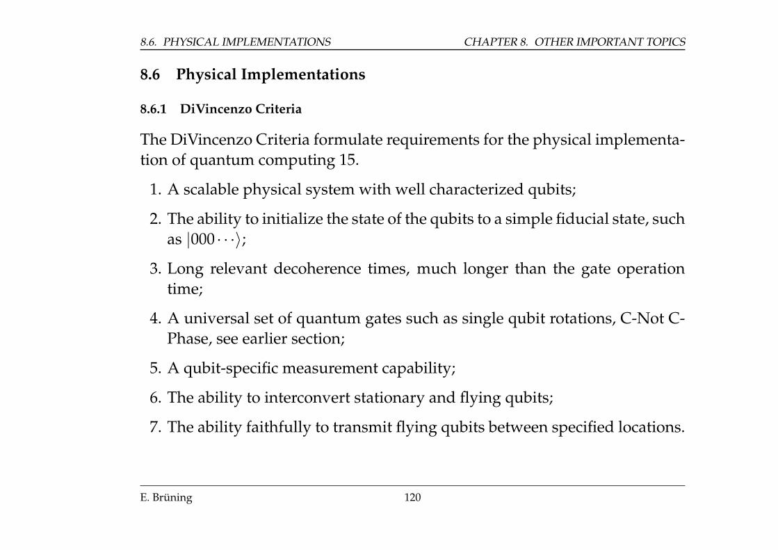
8.6. PHYSICAL IMPLEMENTATIONS CHAPTER 8. OTHER IMPORTANT TOPICS
8.6 Physical Implementations
8.6.1 DiVincenzo Criteria
The DiVincenzo Criteria formulate requirements for the physical implementa-tion of quantum computing 15.
1. A scalable physical system with well characterized qubits;
2. The ability to initialize the state of the qubits to a simple fiducial state, suchas |000 · · ·〉;
3. Long relevant decoherence times, much longer than the gate operationtime;
4. A universal set of quantum gates such as single qubit rotations, C-Not C-Phase, see earlier section;
5. A qubit-specific measurement capability;
6. The ability to interconvert stationary and flying qubits;
7. The ability faithfully to transmit flying qubits between specified locations.
E. Brüning 120
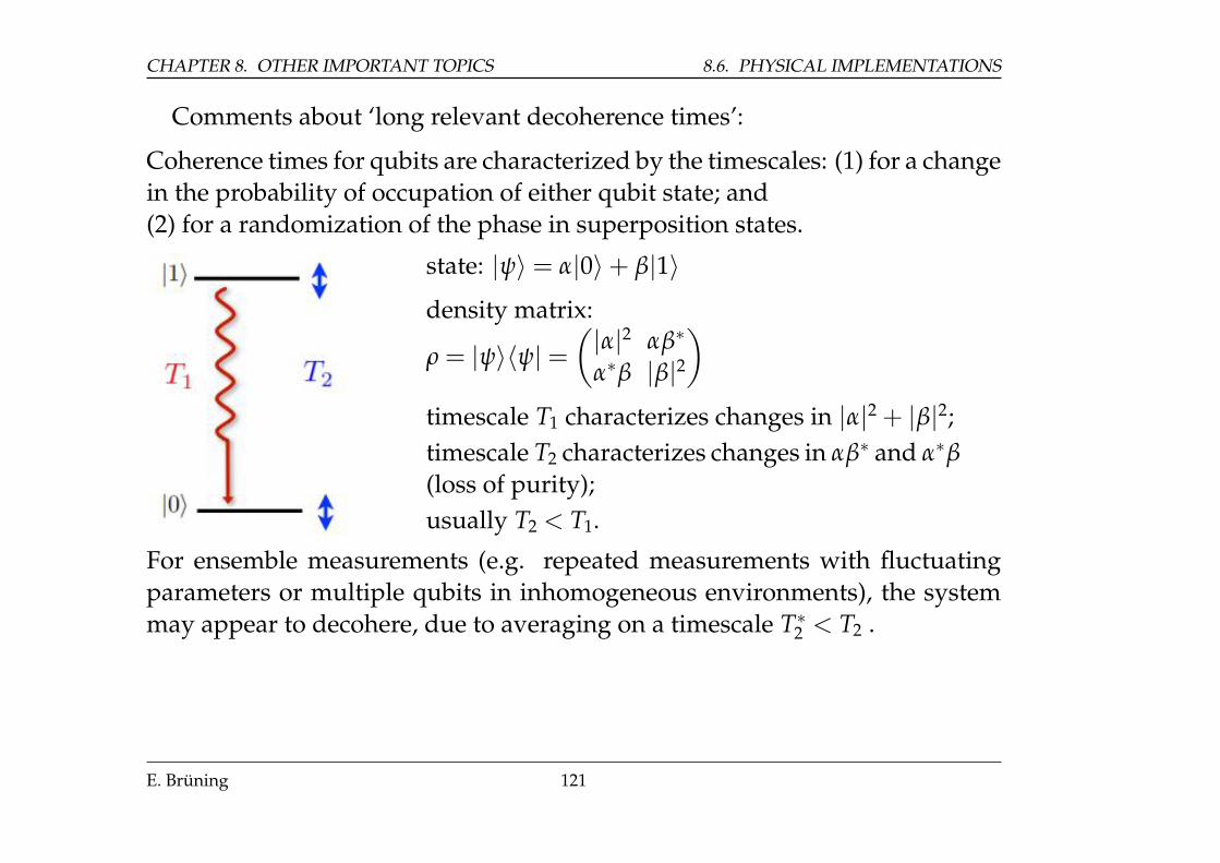
CHAPTER 8. OTHER IMPORTANT TOPICS 8.6. PHYSICAL IMPLEMENTATIONS
Comments about ‘long relevant decoherence times’:
Coherence times for qubits are characterized by the timescales: (1) for a changein the probability of occupation of either qubit state; and(2) for a randomization of the phase in superposition states.
state: |ψ〉 = α|0〉+ β|1〉density matrix:
ρ = |ψ〉〈ψ| =(|α|2 αβ∗
α∗β |β|2)
timescale T1 characterizes changes in |α|2 + |β|2;timescale T2 characterizes changes in αβ∗ and α∗β
(loss of purity);usually T2 < T1.
For ensemble measurements (e.g. repeated measurements with fluctuatingparameters or multiple qubits in inhomogeneous environments), the systemmay appear to decohere, due to averaging on a timescale T∗2 < T2 .
E. Brüning 121
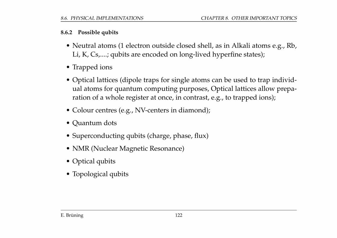
8.6. PHYSICAL IMPLEMENTATIONS CHAPTER 8. OTHER IMPORTANT TOPICS
8.6.2 Possible qubits
• Neutral atoms (1 electron outside closed shell, as in Alkali atoms e.g., Rb,Li, K, Cs,....; qubits are encoded on long-lived hyperfine states);
• Trapped ions
• Optical lattices (dipole traps for single atoms can be used to trap individ-ual atoms for quantum computing purposes, Optical lattices allow prepa-ration of a whole register at once, in contrast, e.g., to trapped ions);
• Colour centres (e.g., NV-centers in diamond);
• Quantum dots
• Superconducting qubits (charge, phase, flux)
• NMR (Nuclear Magnetic Resonance)
• Optical qubits
• Topological qubits
E. Brüning 122
Bibliography
1 C.H. Bennet and S.J. Wiesner. Communication via one- and two-particleoperators on Einstein-Podolsky-Rosen states. Phys. Rev. Lett., 69:2881 – 2884,1992.
2 C. H. Bennett. Quantum cryptography using any two nonorthogonal states.Phys. Rev. Lett., 68:3121 – 3124, 1992.
3 C. H. Bennett and G. Brassard. Proceedings of the IEEEInternational Con-ference on Computers, systems and signal processing, bangalore, india. InProceedings of the IEEE International Conference on Computers, Systems and Sig-nal Processing, Bangalore, India, pages 175 – 179, New York, 1984. IEEE.
4 J.-W. Pan K. Mattle M. Eibl H. Weinfurter Bouwmeester, D. and A. Zeilinger.Experimental quantum teleportation. Nature (London), 390:575, 1997.
123
BIBLIOGRAPHY BIBLIOGRAPHY
5 S.L. Braunstein and H.J. Kimble. Teleportation of Continuous QuantumVariables. Phys. Rev. Lett., 80:869–872, 1998.
6 A.R. Calderbank and B.P. W. Shor. Good quantum error-correcting codesexist. Phys. Rev. A, 54:1086, 1996.
7 C.H. Bennett, C. Crépeau, R. Jozsa, A. Peres, G. Brassard and W.K. Woot-ters. Teleporting unknown quantum state via dual classical and Einstein-Podolsky-Rosen channels. Phys. Rev. Lett., 70:1895, 1993.
8 D. Deutsch. Quantum theory, the Church-Turing Principle and universalquantum computer. Proc. R. Soc. London A, 400:11–20, 1985.
9 D. Deutsch. Conditional quantum dynamics and logic gates. Phys. Rev. Let-ters, 74:4083–4036, 1995.
10 A. Ekert and R. Jozsa. Quantum computation and Shor’s factoring algo-rithm. Reviews of Modern Physics, 68:733 – 753, 1996.
11 R. P. Feynman. Quantum mechanical computers. Optics News,, 11(2):11–20,1985.
E. Brüning 124
BIBLIOGRAPHY BIBLIOGRAPHY
12 Grover L.K. A fast quantum mechanical algorithm for database search. InProceedings, 28th Annual ACM Symposium on the Theory of Computing, page212, 1996.
13 P. W. Shor. Algorithm for quantum computation: discrete logarithms andfactoring. In Proc. 35th Annual Symposium on Foundation of Computer Science,,Los Alamitos CA, 1994. IEEE Press.
14 L. Vaidman. Teleportation of quantum states. Phys. Rev. A, 49:1473 – 1476,1994.
15 P.D. DiVincenzo. The Physical Implementation of Quantum Computation.Fortschritte der Physik, 48:771, 2000.
16 R.F. Werner. All teleportation and dense coding schemes. J. Phys. A: Math.Gen., 34:7081, 2001.
E. Brüning 125

![Building a Quantum Information Processor using ... · [M. Nielsen and I. Chuang, Quantum Computation and Quantum Information (Cambridge, 2000)] • Quantum information processing](https://img.dokumen.tips/doc/110x75/5b8106597f8b9a2a088e3dd6/building-a-quantum-information-processor-using-m-nielsen-and-i-chuang.jpg)