Embed Size (px)
Citation preview

ELY, WILLIAM, M.A. Pricing European Stock Options using Stochastic and FuzzyContinuous Time Processes. (2012)Directed by Jan Rychtar. 71 pp.
Over the past 40 years, much of mathematical nance has been built on the
premise that stocks tend to move according to continuous-time stochastic processes,
particularly geometric Brownian Motion. However, fuzzy set theory has recently been
shown to hold promise as a model for nancial uncertainty as well, with continuous
time fuzzy processes used in place of Brownian Motion. And, like Brownian Motion,
fuzzy processes also cannot be measured using a traditional Lebesque integral. This
problem was solved on the stochastic side with the development of Ito's calculus.
Likewise, the Liu integral has been developed to measure fuzzy processes. In this
thesis we will describe and compare the theoretical underpinnings of these models, as
well as "back-test" several variations of them on historical market data.

PRICING EUROPEAN STOCK OPTIONS USING STOCHASTIC AND FUZZY
CONTINUOUS TIME PROCESSES
by
William Ely
A Thesis Submitted tothe Faculty of the Graduate School at
The University of North Carolina at Greensboroin Partial Fulllment
of the Requirements for the DegreeMaster of Arts
Greensboro2012
Approved by
Committee Chair

APPROVAL PAGE
This thesis has been approved by the following committee of the Faculty of The
Graduate School at The University of North Carolina at Greensboro.
Committee ChairJan Rychtar
Committee MembersMaya Chhetri
Sat Gupta
Date of Acceptance by Committee
Date of Final Oral Examination
ii

TABLE OF CONTENTS
Page
LIST OF TABLES . . . . . . . . . . . . . . . . . . . . . . . . . . . . . . . . . . . . . . . . v
LIST OF FIGURES . . . . . . . . . . . . . . . . . . . . . . . . . . . . . . . . . . . . . . . vi
CHAPTER
I. INTRODUCTION . . . . . . . . . . . . . . . . . . . . . . . . . . . . . . . . . . 1
1.1. Overview and Rationale . . . . . . . . . . . . . . . . . . . . . . . . . . 11.2. Organization of Thesis . . . . . . . . . . . . . . . . . . . . . . . . . . . 2
II. BLACK SCHOLES MODEL . . . . . . . . . . . . . . . . . . . . . . . . . . . 3
2.1. Probability Measure . . . . . . . . . . . . . . . . . . . . . . . . . . . . 32.2. European Call Option . . . . . . . . . . . . . . . . . . . . . . . . . . . 82.3. Black Scholes Model . . . . . . . . . . . . . . . . . . . . . . . . . . . . 92.4. Stochastic Volatility . . . . . . . . . . . . . . . . . . . . . . . . . . . . 13
III. LIU MODEL . . . . . . . . . . . . . . . . . . . . . . . . . . . . . . . . . . . . . 14
3.1. Credibility Measure . . . . . . . . . . . . . . . . . . . . . . . . . . . . . 143.2. Liu Process . . . . . . . . . . . . . . . . . . . . . . . . . . . . . . . . . . 263.3. Liu's Stock Model . . . . . . . . . . . . . . . . . . . . . . . . . . . . . . 293.4. Gao's Stock Model . . . . . . . . . . . . . . . . . . . . . . . . . . . . . 32
IV. QUANTITATIVE COMPARISON . . . . . . . . . . . . . . . . . . . . . . . 34
4.1. Purpose . . . . . . . . . . . . . . . . . . . . . . . . . . . . . . . . . . . . 344.2. Procedure . . . . . . . . . . . . . . . . . . . . . . . . . . . . . . . . . . . 344.3. Data Analysis . . . . . . . . . . . . . . . . . . . . . . . . . . . . . . . . 364.4. Hypothesis Testing . . . . . . . . . . . . . . . . . . . . . . . . . . . . . 38
V. RESULTS . . . . . . . . . . . . . . . . . . . . . . . . . . . . . . . . . . . . . . . 40
5.1. Visual Example . . . . . . . . . . . . . . . . . . . . . . . . . . . . . . . 415.2. Data for Each Trial . . . . . . . . . . . . . . . . . . . . . . . . . . . . . 435.3. Discussion . . . . . . . . . . . . . . . . . . . . . . . . . . . . . . . . . . . 50
iii

VI. CONCLUSION . . . . . . . . . . . . . . . . . . . . . . . . . . . . . . . . . . . . 54
REFERENCES . . . . . . . . . . . . . . . . . . . . . . . . . . . . . . . . . . . . . . . . . . 55
APPENDIX A. MATLAB CODE . . . . . . . . . . . . . . . . . . . . . . . . . . . . . . 57
APPENDIX B. GLOSSARY . . . . . . . . . . . . . . . . . . . . . . . . . . . . . . . . . 69
iv

LIST OF TABLES
Page
Table 1. Notation for Black Scholes formula (II.14). . . . . . . . . . . . . . . . 11
Table 2. Example 30-Day Trial . . . . . . . . . . . . . . . . . . . . . . . . . . . . . 38
Table 3. ARMSE for 30 Day Trial . . . . . . . . . . . . . . . . . . . . . . . . . . . 43
Table 4. AMAE for 30 Day Trial . . . . . . . . . . . . . . . . . . . . . . . . . . . . 43
Table 5. ARMSE for 60 Day Trial . . . . . . . . . . . . . . . . . . . . . . . . . . . 44
Table 6. AMAE for 60 Day Trial . . . . . . . . . . . . . . . . . . . . . . . . . . . . 44
Table 7. ARMSE for 90 Day Trial . . . . . . . . . . . . . . . . . . . . . . . . . . . 45
Table 8. AMAE for 90 Day Trial . . . . . . . . . . . . . . . . . . . . . . . . . . . . 45
Table 9. ARMSE for 120 Day Trial . . . . . . . . . . . . . . . . . . . . . . . . . . 46
Table 10. AMAE for 120 Day Trial . . . . . . . . . . . . . . . . . . . . . . . . . . . 46
Table 11. ARMSE for 150 Day Trial . . . . . . . . . . . . . . . . . . . . . . . . . . 47
Table 12. AMAE for 150 Day Trial . . . . . . . . . . . . . . . . . . . . . . . . . . . 47
Table 13. ARMSE for 180 Day Trial . . . . . . . . . . . . . . . . . . . . . . . . . . 48
Table 14. AMAE for 180 Day Trial . . . . . . . . . . . . . . . . . . . . . . . . . . . 48
Table 15. ARMSE for 210 Day Trial . . . . . . . . . . . . . . . . . . . . . . . . . . 49
Table 16. AMAE for 210 Day Trial . . . . . . . . . . . . . . . . . . . . . . . . . . . 49
Table 17. ARMSE for 240 Day Trial . . . . . . . . . . . . . . . . . . . . . . . . . . 50
Table 18. AMAE for 240 Day Trial . . . . . . . . . . . . . . . . . . . . . . . . . . . 50
v

LIST OF FIGURES
Page
Figure 1. CPB Call Option, Actual and Predicted Values . . . . . . . . . . . . 42
Figure 2. CPB Call Option, Error Terms over Time . . . . . . . . . . . . . . . 42
Figure 3. Normal Fuzzy vs. Normal Random . . . . . . . . . . . . . . . . . . . . 53
vi

CHAPTER I
INTRODUCTION
1.1 Overview and Rationale
Today's nancial markets trade in a wide variety of nancial instruments. These
are typically divided into underlying assets (commodities, foreign currency, stocks,
bonds) and derivatives whose values are based on some underlying asset. These
include basic options like call options and put options (the right to buy/sell an asset
at a certain price in the future), as well as more complex instruments like interest-
rate swaps and the now-infamous mortgage-backed securities. Derivatives have many
uses in modern nancial markets, not only as speculative tools, but also as insurance
against uncertainty. A manufacturer of gold watches might want to insure himself
against a rise in the price of gold by purchasing a call option on gold, and a borrower
could protect themselves from a rise in interest rates by purchasing an interest rate
swap to lock in a particular rate. Because of their profusion and utility in today's
markets, the pricing of these derivatives has become a primary concern of modern
mathematical nance.
Because a derivative's price is based partly on the future price of the underlying
asset, there is an element of uncertainty involved in pricing. For this reason, pricing
models typically include some amount of randomness. One of the most important
models, the Black Scholes Model [2], is based on the assumption that stock prices can
1

be modeled using a stochastic process over a probability space. However, there are
several other approaches to options modeling, including the one proposed by Baoding
Liu [20]. Instead of the traditional probability measure, he denes the Credibility
Measure and a "fuzzy process" as a possible model for the movement of stock prices.
This thesis concerns itself with a theoretical and practical comparison of these two
models.
1.2 Organization of Thesis
We begin with a brief overview of probability measure and an introduction to
Brownian Motion and its applications in nance in Chapter 2. This will introduce the
rationale and formula for the Black Scholes model. This portion of the thesis contains
a review of existing literature on the topic. In Chapter 3 we develop the Credibility
Measure as an alternative measure of uncertainty, and see that fuzzy processes can
also be used in nancial modeling. This chapter concludes with the derivation of the
Liu model. While signicant literature exists on the topic of fuzzy processes ([20],
[14], [15], [18], [17], [16], [5]) this portion of the thesis represents a self-contained,
original axiomatic compilation. In Chapter 4, a quantitative comparison between the
Black Scholes and Liu model is performed, with results and implications discussed in
Chapter 5. In my review of the literature on fuzzy processes in nance, we have not
encountered a similar comparison. As an appendix, we have included MATLAB code
used for my quantitative comparison.
2

CHAPTER II
BLACK SCHOLES MODEL
2.1 Probability Measure
Denition II.1 (σ-Algebra, [21]). A collection F of subsets of a set Ω is said to be
a σ-algebra in Ω if F has the following properties:
(1) Ω ∈ F .
(2) If A ∈ F then Ac ∈ F , where Ac is the complement of A relative to Ω.
(3) If A =⋃∞n=1An and if An ∈ F for n = 1, 2, 3, ...., then A ∈ F .
Denition II.2 (Probability Space, [3]). A probability space is an ordered triple
(Ω,F , P ), where Ω is any non-empty set, F is a σ-algebra on Ω and P : F → [0, 1] is
a probability measure on F such that
(1) P (Ω) = 1 and P (∅) = 0
(2) for any countable collection Ai∞i=1 ⊂ F with Ai⋂Aj = ∅, i 6= j:
P
(∞⋃i=1
Ai
)=∞∑i=1
P (Ai) (II.1)
We call Ω the sample space, the elements of F events and each element of Ω an
elementary event.
3

In dening a random variable, we wish to assign a numerical value X(ω) ∈ [0, 1]
to every elementary element ω ∈ Ω.
Denition II.3 (Measurable function, [21]). Let E be a set and F be a σ-algebra
on E. Then a function X : (E,F) → R is called (Borel) measurable if X−1(B) ∈ F
for all B ∈ BR, where BR is the Borel σ-algebra generated by open intervals in R.
Denition II.4 (Random Variable, [3]). Let (Ω,F , P ) be a probability space. Then
a Borel-measurable mapping X : (Ω,F , P )→ R is a called random variable.
This allows us to measure the probability that the random variable will take on
values in any B ∈ BR.
Denition II.5 (Independent Random Variables, [24]). Let (Ω,F , P ) be a probabil-
ity space, with Fi be a sub-σ-algebra for i in some non-empty index set I. Then the
σ-algebras Fi are said to be mutually P-independent if for every subset i1, ..., in ⊂ I
and every choice Aim ∈ Fim , 1 ≤ m ≤ n, we have:
P (Ai1 ∩ .. ∩ Ain) = P (Ai1) ∗ ... ∗ P (Ain) (II.2)
It should be noted that the more traditional denition of independence is that
two sets A and B are independent if P (A ∩ B) = P (A)P (B) and that these two
denitions are equivalent.
For the purposes of this thesis, we will be considering only discrete time processes
indexed by t ∈ N and continuous time processes indexed over R+ = [0,∞). In any
4

case, our index set T will have a natural σ-algebra of Borel sets inherited from R.
Consequently, T × Ω will have a product σ-algebra [21, Denition 7.1].
Denition II.6 (Stochastic Process, [10]). Given a probability space (Ω,F , P ), an
index set T (T = N or T = [0,∞)) a stochastic process is a measurable function
X : T × Ω→ R.
In particular, if X is a stochastic process, then
(i) X(t, .) : Ω→ R is a random variable, denoted Xt.
(ii) X(., ω) : T → Ω is a measurable function.
Denition II.7 (Sample path, [3]). Given a stochastic process X : T × Ω→ R and
ω ∈ Ω, the sample path of ω is a function t→ X(t, ω).
Denition II.8 (Brownian Motion, [10]). A stochastic process B(t, ω) is called a
Brownian motion if it satises the following conditions:
(1) Pω|B(0, ω) = 0 = 1.
(2) For any 0 ≤ s < t, Bt−Bs is a normally distributed random variable with mean
0 and variance t− s Here, by Bt −Bs we mean a function from Ω to R that to
each ω ∈ Ω assigns a value B(t, ω)−B(s, ω)., s.t. for any a < b
Pa ≤ Bt −Bs ≤ b =1√
2π(t− s)
∫ b
a
e−x2
2(t− s)dx (II.3)
5

(3) B(t, ω) has independent increments. This means that for any 0 ≤ t1 < t2 <
.. < tn, the random variables
Bt1 , Bt2 −Bt1 , ..., Btn −Btn−1 (II.4)
are independent.
(4) Almost all sample paths of B(t, ω) are continuous functions. This means that
Pω|B(., ω) is continuous = 1 (II.5)
Brownian motion provides us with a good framework for describing the behavior of
a stock price - jumps in price occur (particularly in today's computer-driven markets)
nearly instantaneously, and with a large degree of randomness. However, there are
several problems with the use of standard Brownian motion to describe investments.
First, standard Brownian motion can take on negative values, whereas a stock price
does not. Second, nancial markets do not operate completely randomly - the stock
price tends to "drift" in a certain direction despite its randomness in the short-term.
Thus the geometric Brownian motion was proposed, with the stock price tending to
follow the stochastic dierential equation [11]:
dStSt
= µdt+ σdWt (II.6)
6

The dt term here represents the change in time over which we are observing the
stock, and mimics a standard dierential equation. Over time, we see a change in the
price represented by the parameter µ, referred to as drift. This takes into account
the fact that, over time, stocks experience a constant pull upwards, measured as the
rate of return on a risk-less asset.
However, we also have our stock price aected by the term σdWt. The dWt here is
the stochastic part of the dierential equation, and can be described as the change in
the path of a standard Brownian motion over an interval of length t as t→ 0+. This
stochastic element models the random behavior of the future stock price, with the
parameter σ denoting the magnitude of expected uncertainty. The σ used is known as
volatility, which is calculated as the standard deviation of the stock's rate of return,
and though constant in the basic model, can also vary over time and price.
Intuitively, the stochastic dierential equation provides a good way of explaining
the relationship between the price of the stock and both the deterministic and Brow-
nian elements of its movement. However this equation is really an informal way of
expressing the integral
St+s − St =
∫ t+s
t
µ(Xu, u)du+
∫ t+s
t
σ(Xu, u)dBu (II.7)
where∫ t+st
µ(Xu, u)du is a traditional Lebesgue integral taken over the deterministic
path of our stock's "drift" and∫ t+st
σ(Xu, u)dBu is integrated over the path of a
standard Brownian motion. Because the path of a Brownian motion is nowhere
dierentiable [10], standard integration cannot produce a solution to the dierential
7

equation. It was only with the work of Ito that such integrals became manageable
through the process of stochastic integration [19]. The steps for constructing the Ito
integral are given a very thorough treatment in Kuo, 2006 [10]. However, the basic
process can be understood in parallel to the construction of the Lebesgue integral
[21].
2.2 European Call Option
The most basic of stock options is the European call option, giving the bearer the
right to buy a given stock at a specied price (called the "strike price" at a specic
date in the future (called the "expiration date"). If the price of the stock on the
expiration date (called the "spot price") is greater than the strike price, the bearer
can exercise the option, buy the stock at the strike price, and then sell it at the
current price, netting a gain of (price - strike) on the expiration date. An option that
can be exercised for a gain is called "in-the-money." On the other hand, if the stock
price is lower than the strike price, there is no gain in exercising the option, and it is
called "out-of-the-money." Thus the payo on a European call option can be dened
by max[0, (P −K)] for K =strike price and P =price at expiration (also referred to
as "spot price").
In order to compute the actual prot made on the purchase of such an option, we
also have to take into account the cost of the option. And because the payo will
not occur until the exercise date at some point in the future, we must consider the
potential interest that could have been earned had the price of the premium been
invested in a risk-free asset for that time period. Thus the prot on a call option is
8

given by:
Prot = max[0, (P −K)]− Future Value[Option Price] (II.8)
where the future value of money is simply the value of that amount invested at
the risk-free rate for the specied period of time. It is generally calculated using
continuously-compounded interest, so that $A invested at a risk free rate r for t years
would have value $Aert [19].
2.3 Black Scholes Model
Binomial Option Pricing
Consider a stock S, priced at $55, which can take on one of two values at the end
of one year, say $65 and $45. We wish to determine the value of an option expiring
in one year, with strike price K = 50 and assuming a risk-free interest rate of .06. In
order to do this, we will create and price a "synthetic option" by borrowing at the
risk-free rate and purchasing an amount of stock so that, in one year, the payo to
the synthetic option will be equal to the payo from the call option. The Law of One
Price [19] states that positions with equal payos will have equal price, and so the
price of our synthetic option will be the same as the option we are interested in.
Since our stock can take on only two values, we know that there are two possible
payos for our option: Pu = $15 if the stock goes up and Pd = $0 if the stock goes
down (since the option will not be exercised). We want to buy ∆ shares of stock
and "borrow" $B at the risk-free rate r such that our portfolio has equal payo (a
negative value for $B implies that we will be loaning that amount). Assuming our
9

stock pays a dividend of δyear
, we see that our ∆ and B must satisfy the equations:
(∆ ∗ 45 ∗ eδ) + (B ∗ er) = 0 (II.9)
(∆ ∗ 65 ∗ eδ) + (B ∗ er) = 15 (II.10)
We can in fact solve for ∆ and B for a stock with current price $S over any period
h. Let Sd be the stock price after a downward move, Su be the price after an upward
move, Pd be the payo of an option of strike price K after a downward move, Pu the
payo after an upward move. For u = SuSand d = Sd
Swe have [19]:
∆ = e−δhPu − PdS(u− d)
(II.11)
B = e−rhuPd − dPc
(u− d)(II.12)
Call Price = ∆S +B (II.13)
And we see that, in our case (letting δ = 0), ∆ = 12and B = $− 21.1897. Thus our
option would cost ∆S +B = $6.3103.
Needless to say, a single up/down movement per year is not realistic for any stock.
However, as the period h approaches zero, we see not only that the binomial model
begins to look more plausible, but also mimics the random walk on which Brownian
motion is based. It can be shown that, as h → 0+, the prices predicted by the
binomial model are the same as those predicted by the Black Scholes Model [7]. The
interested reader should consult MacDonald's Derivatives Markets [19] for a more
10

thorough treatment of the binomial stock model.
Black Scholes Formula, [2]
The solution to the stochastic dierential equation (II.6) yields a formula for
pricing call options and glsplput (and which can be modied to price a variety of
other options). Inputs for the formula are given in the Table 1
Table 1. Notation for Black Scholes formula (II.14).
Symbol Meaning
S current stock price
K option strike price
σ volatility of stock (calculated as standard deviation of rate of return)
r continuously compounded risk-free annual interest rate
T time to expiration
δ annual dividend yield for stock
The price of a call option is then given by:
Price = Se−δTN(d1)−Ke−rTN(d2), where (II.14)
d1 =ln( S
K) + (r − δ + 1
2σ2)T
σ√T
(II.15)
d2 = d1 − σ√T (II.16)
11

and N(x) is the cumulative distribution function for the Normal distribution, dened
[19]
N(x) =1
σ√
2π
∫ x
−∞exp
(−t2
2
)dt (II.17)
which represents the probability that a standard normal random variable will take
a value in the interval (−∞, x].
Assumptions of Black Scholes
The original Black-Scholes formula (II.14) is based on a set of assumptions about
the nancial markets in which the option is traded.
(1) There is a constant, known interest rate at which it is possible to lend and
borrow cash.
(2) It is possible to buy and sell any amount, including fractions of shares, of stock.
(3) There are no transaction costs (such as brokerage fees or bid-ask spreads).
(4) The stock price follow geometric Brownian motion with a constant volatility
and a drift that is both constant and equal to the risk free rate.
While these assumptions render the formula somewhat impractical, more current
developments have been made to account for violations of these assumptions in the
real world. Newer models, for example, include a term for continuous dividend yield,
and other extensions have been made to handle discrete dividends and non-constant
12

volatility. Particularly, it has been theorized that a stock's volatility, rather than
remaining constant, behaves stochastically.
2.4 Stochastic Volatility
There are several extensions which allow for stochastic volatility within the orig-
inal Black Scholes framework. Hull and White [8] and Wiggins [28] developed early
extensions in which volatility behaves stochastically, but is uncorrelated to spot price.
These models have shown to behave similarly to Black Scholes, though with slightly
better accuracy on options with longer time to maturity [8], [28]. Another impor-
tant stochastic volatility model was then developed by Heston [6] who added the
assumption that volatilities are not only stochastic, but correlated with spot price.
These more sophisticated models can often provide a higher degree of predictive
accuracy than the original Black-Scholes model. However, the purpose of this thesis
is not forecasting, but rather to gain insight into the behavioral dierences between
stochastic and fuzzy processes. Thus we restrict ourselves to models with constant
volatility for both simplicity and clarity.
Having now described the basic probabilistic models for option pricing, we move
to those models established through fuzzy set theory.
13

CHAPTER III
LIU MODEL
3.1 Credibility Measure
Zadeh [29] initially introduced the possibility measure to deal with fuzzy events,
assigning a value between 0 and 1 to a fuzzy event based on its "grade of membership."
However, the possibility measure lacks the very useful property of self-duality (i.e.
Pos A + Pos Ac 6= 1 for all A ⊂ Ω), and so Liu and Liu [18] proposed the
credibility measure as an alternative way to measure fuzzy events.
It should be noted that the possibility and credibility "measures" referred to in
this thesis do not adhere to the countable additivity of traditional measure theory.
For this reason, we cannot use the framework of standard measure theory, and must
instead establish several useful properties axiomatically.
We construct credibility in terms of possibility, and thus some information about
the possibility measure is rst necessary.
Denition III.1. For a set Ω and its power set P(Ω), we dene a function Pos :
P(Ω)→ [0, 1] to be a possibility measure if:
(1) Pos Ω = 1
(2) Pos ∅ = 0
(3) Pos ⋃iAi = supi Pos Ai for any countable collection Ai in P(Ω)
14

Denition III.2. For a set Ω and its power set P(Ω), we dene the necessity of a
set A ∈ P(Ω) to be NecA = 1− Pos Ac.
In order to create a possibility measure, let us take a function µ : Ω→ [0, 1] with
supx∈Ω
µ(x) = 1. (III.1)
For example let Ω = [0, 2] and µ(x) = x2.
Theorem III.3 (Existence of a Possibility measure). Let µ : Ω→ [0, 1] is a function
satisfying (III.1). Then the function Pos : P(Ω)→ [0, 1] dened by
Pos A = supx∈A
µ(x) (III.2)
is a possibility measure.
Proof. 1. Pos Ω = supx∈Ω µ(x) = 1.
2. Pos ∅ = 0 by convention i.e. supx∈∅ µ(x) = 0.
3. We begin by letting
α = Pos
⋃i
Ai
= sup
x∈⋃∞i Ai
µ(x) (III.3)
and
β = supiPos Ai = sup(sup
x∈Aiµ(x)). (III.4)
15

Now assume, by way of contradiction, that α 6= β. If α < β then there must
be i0 such that supx∈Ai0 µ(x) > α = supx∈⋃Aiµ(x) But this is impossible because
Ai0 ⊂⋃Ai.
We then consider the case of α > β. This implies that α + ε0 = β for some
ε0 > 0. α = supx∈⋃∞i Aiµ(x) and so for ε0
2there exists some x0 ∈
⋃∞i Ai such that
|α− µ(x0)| < ε (or else α would not be the least upper bound). This implies that
µ(x0) > α− ε02> β = sup(sup
x∈Aiµ(x) for all i ∈ N). (III.5)
But x0 is in some Ai and so we have a contradiction. Thus we have α = β.
Theorem III.4. For A ⊂ B ⊂ Ω, Pos A ≤ Pos B.
Proof. Assume, by way of contradiction, that Pos A > Pos B, say Pos A+ε0 =
Pos B with ε0 > 0. Then for ε02there must exist x0 ∈ A s.t |Pos A− µ(x0)| < ε0
2.
Then for x0 ∈ A ⊂ B we have µ(x0) > supx∈B µ(x), a contradiction. Thus Pos A ≤
Pos B.
Corollary III.5. If Pos A < 1, then Pos Ac = 1.
Proof. (A⋃Ac) = Ω and so Pos A
⋃Ac = Pos Ω = 1. But
PosA⋃
Ac
= sup(Pos A ,Pos Ac) (III.6)
and Pos A < 1 so Pos Ac = 1.
16

Now that we have constructed a Possibility Measure, we will use it to create a
Credibility Measure. First we outline the properties that we wish for our Credibility
Measure to have.
Denition III.6 (Credibility Measure, [20]). For a set Ω and its power set P(Ω),
with A,B ∈ P(Ω) , we dene a function Cr : P(Ω)→ [0, 1] to be a credibility measure
if it satises the following conditions:
Axiom 1. Normality: Cr Ω = 1.
Axiom 2. Monotonicity: Cr A ≤ Cr B whenever A ⊂ B ⊂ Ω.
Axiom 3. Self-Duality: Cr A+ Cr Ac = 1 for any A ⊂ Ω.
Axiom 4. Maximality: Cr ⋃iAi = supiCr Ai for any countable collection Ai
with supiCr Ai < 0.5.
We now show that a Credibility Measure exists.
Theorem III.7 (Existence of credibility Measure). Let Ω be a set, µ : Ω → [0, 1]
satisfying (III.1) and Pos be a function given by (III.2). Then a function Cr :
P(Ω)→ [0, 1] for A ∈ P(Ω), dened by
Cr A =1
2(Pos A+ 1− Pos Ac) (III.7)
is a credibility measure on Ω.
Proof. We now show that a function, dened by (III.7), satises the four axioms
above.
17

Normality: Cr Ω = 12(Pos Ω+ 1− Pos ∅) = 1
Monotonicity: Take any A,B ∈ P(Ω) with A ⊂ B. Then, by (III.4) Pos A ≤
Pos B. We also have Bc ⊂ Ac and so
(1− Pos Ac) ≤ (1− Pos Bc). (III.8)
(Pos A+ 1− Pos Ac) ≤ (Pos B+ 1− Pos Bc) (III.9)
And thus Cr A ≤ Cr B
Self-Duality:
Cr A+ Cr Ac =
1
2(Pos A+ 1− Pos Ac) +
1
2(Pos Ac+ 1− Pos A)
=1
2(2) = 1
Maximality(Cr ⋃iAi = supiCr Ai for countable Ai with supiCr Ai <
0.5):
If Cr ⋃iAi < 0.5 then
Pos
⋃i
Ai
< Pos
(⋃i
Ai)c
. (III.10)
18

Then by Corollary 1 we have
Pos
(⋃i
Ai)c
= 1⇒ Cr
⋃i
Ai
=
1
2Pos
⋃i
Ai
(III.11)
=1
2supiPos Ai = sup
iCr Ai (III.12)
And so we have
Cr
⋃i
Ai
= sup
iCr Ai (III.13)
We see that credibility is dened as the average of a subsets possibility and ne-
cessity.
Lemma III.8. Let Pos be possibility and Cr be given by (III.7). For A ⊂ Ω with
Cr A < 0.5, then Pos A < Pos Ac.
Proof. For Cr A = 12(Pos A + 1 − Pos Ac) < 0.5 we have (Pos A + 1 −
Pos Ac) < 1 and so Pos A < Pos Ac.
Theorem III.9. [14] Possibility measures and credibility measures are uniquely de-
termined by each other via (III.7). Furthermore:
Pos A = (2Cr A) ∧ 1 (III.14)
for any A ⊂ Ω.
19

Proof. We have already determined a credibility measure using possibility (III.7).
Now we wish to show that if two possibility measures, Pos1 A and Pos2 A, both
give the same credibility, then these possibility measures must be equal i.e. if for all
A ⊂ Ω
Cr A =1
2(Pos1 A+ 1− Pos1 Ac) and (III.15)
Cr A =1
2(Pos2 A+ 1− Pos2 Ac), (III.16)
then Pos1 A = Pos2 A .
Fix A ⊂ Ω
Case 1: (Pos1 A = 1 and Pos2 A < 1)
If Pos2 A < 1 then Pos2 Ac = 1 ⇒ Pos2 A − Pos2 Ac < 0. Then for
Pos1 A = 1 we have Pos1 Ac ≤ 1 ⇒ Pos1 A − Pos1 Ac ≥ 0. Then by our
assumption
1
2(Pos1 A+1−Pos1 Ac) =
1
2(Pos2 A+1−Pos2 Ac), which implies (III.17)
Pos1 A − Pos1 Ac = Pos2 A − Pos2 Ac (III.18)
and so we have
Pos1 A − Pos1 Ac ≥ 0 > Pos2 A − Pos2 Ac (III.19)
20

This contradicts our assumption of equality. Similar reasoning works if Pos A1 <
1 and Pos A2 = 1.
Case 2: (Pos1 A < 1 and Pos2 A < 1): Pos1 A < 1 and so by Corollary 1
we have Pos1 Ac = 1. By the same reasoning, Pos2 A < 1 implies Pos2 Ac = 1.
By our assumption that
1
2(Pos1 A+ 1− Pos1 Ac) =
1
2(Pos2 A+ 1− Pos2 Ac), (III.20)
we now have Pos1 A − 1 = Pos2 A − 1 or Pos1 A = Pos2 A.
And so possibility is uniquely determined by credibility.
Now we wish to show Pos A = (2Cr A)∧ 1. First consider the case Cr A <
0.5. This implies that Pos A < Pos Ac, and so by Corollary 1 Pos Ac = 1 and
so Pos A = 2Cr A. For Cr A ≥ 0.5, by (III.7) we must have Pos A = 1 and
thus Pos A = (2Cr A) ∧ 1.
Denition III.10 (Fuzzy Variable [20]). A fuzzy variable is a function from a cred-
ibility space (Ω,P(Ω), Cr) to the set of real numbers. [16]
Denition III.11 (Membership Function [20]). Let ξ be a fuzzy variable dened on
the credibility space (Ω,P(Ω), Cr). Then it's membership function is dened by
µξ(x) = (2Cr ξ = x) ∧ 1 (III.21)
21

Theorem III.12 (Credibility Inversion Theorem, [17]). Let ξ be a fuzzy variable with
membership function µξ. Then for any B ⊂ R
Cr ξ ∈ B =1
2
(supx∈B
µξ(x) + 1− supx∈Bc
µξ(x)
)(III.22)
Where Cr ξ ∈ B represents the "likelihood" that the fuzzy variable ξ will take a value
in B.
We have thus far shown that there exist unique relationships between a credibility
measure, possibility measure and membership function. Given one of these three, we
can uniquely determine the other two.
Denition III.13. A fuzzy variable ξ is said to be normally distributed if it has
associated membership function:
µξ(x) = 2
(1 + exp
(π|x− α|√
6σ
))−1
(III.23)
Denition III.14 (Independent Fuzzy Variables [13]). Fuzzy sets ξ1, .., ξn are said
to be independent if
Cr
n⋂i=1
ξi ∈ Bi
= min
1≤i≤nCr ξi ∈ Bi (III.24)
for all Bi ∈ P(Ω).
22

Denition III.15 (Identically-Distributed Fuzzy Variables [13]). Two fuzzy variables
ξ and ν are said to be identically-distributed if
Cr ξ ∈ B = Cr ν ∈ B (III.25)
for all B ∈ P(Ω).
Denition III.16 (Expected Value, [18]). For a fuzzy variable ξ, the expected value
is dened by
E [ξ] =
∫ +∞
0
Cr ξ ≥ r dr −∫ 0
−∞Cr ξ ≤ r dr (III.26)
so long as at least one of the integrals is nite. If both integrals are innite, the
expected value is undened.
Theorem III.17. [27] Let ξ be a continuous fuzzy variable with membership function
µξ. If the expected value exists, and there is a point x0 such that µξ(x) is increasing
on (−∞, x0) and decreasing on (x0,+∞), then
E [ξ] = x0 +1
2
∫ +∞
x0
µξ(x)dx− 1
2
∫ x0
−∞µξ(x)dx (III.27)
Proof. Consider x0 ≥ 0. Then by (III.12) we have
Cr ξ ≥ r =1
2
(sup
x∈R|x≥rµξ(x) + 1− sup
x∈R|x<rµξ(x)
)(III.28)
23

By our assumption, µξ(x0) > µξ(x)∀x ∈ R and so µξ(x0) = 1. Thus for 0 ≤ r ≤ x0
we have Cr ξ ≥ r = 12
(1 + 1− µξ(x)). For x0 < r we have supx∈R|x<r µξ(x) = 1
which implies Cr ξ ≥ r = 12µξ(x). Likewise, x0 6∈ (−∞, 0) and so Cr ξ ≤ r =
12µξ(x) for r < 0. We can now re-write
E [ξ] =
∫ +∞
0
Cr ξ ≥ r dx−∫ 0
−∞Cr ξ ≤ r dx (III.29)
=
∫ x0
0
Cr ξ ≥ r dx+
∫ +∞
x0
Cr ξ ≥ r dx−∫ 0
−∞Cr ξ ≤ r dx
=
∫ x0
0
(1− 1
2µξ(x))dx+
∫ ∞x0
1
2µξ(x)dx−
∫ 0
−∞
1
2µξ(x)dx
=
∫ x0
0
1dx−∫ x0
0
1
2µξ(x)dx+
∫ ∞x0
1
2µξ(x)dx−
∫ 0
−∞
1
2µξ(x)dx
= x0 +
∫ ∞x0
1
2µξ(x)dx−
∫ x0
−∞
1
2µξ(x)dx
Similar reasoning show this to be true for x0 < 0.
Lemma III.18. Let ξ be a continuous fuzzy variable with membership function µξ.
If the expected value exists, and there is a point x0 such that µξ(x) is increasing on
(−∞, x0) and decreasing on (x0,+∞), with µξ(x) symmetrical on the line x = x0 we
have E [ξ] = x0.
Proof. By (III.17), we know that E [ξ] = x0 +∫∞x0
12µξ(x)dx−
∫ x0−∞
12µξ(x)dx. Likewise,
because µξ(x) is symmetrical about x0 we know that µξ(x0 + x) = µξ(x0− x)∀x ∈ R.
24

This means that∫∞x0
12µξ(x)dx =
∫ x0−∞
12µξ(x)dx and the proof is complete.
Theorem III.19. For a fuzzy variable ξ with normal membership function (III.23),
we have E [ξ] = α.
Proof. Using the theorem and lemma above, we need only to show that µξ(x) =
2(
1 + exp(π|x−α|√
6σ
))−1
is increasing on (−∞, α), decreasing on (α,+∞) and sym-
metric about α. We begin by calculating the derivative of µξ(x).
µ′ξ(x) =
√23π(α− x)e
π√
(α−x)2√6σ
σ√
(α− x)2
(eπ√
(α−x)2√6σ
)2 (III.30)
This equation is positive for x ∈ (−∞, α) and negative for x ∈ (α,+∞) and equals
zero at x = α. Likewise, looking at µξ(x), we see that µ(α + x) = µ(α − x)∀x ∈ R
and so the proof is complete.
Denition III.20 (Variance, [18]). Let ξ be a fuzzy variable with nite expected
value α. Then the variance of ξ is dened by Var [ξ] = E [(ξ − α)2] .
Example III.21. Let ξ be a fuzzy variable with normal membership function
µξ(x) = 2
(1 + exp
(π|x− α|√
6σ
))−1
(III.31)
25

Then the variance of ξ is calculated:
Var [ξ] = E[(ξ − e)2
]=
∫ ∞0
Cr
(ξ − α)2 ≥ rdr
=
∫ ∞0
Cr
(ξ ≥ α +√r) ∪ (ξ ≤ α−
√r)dr
=
∫ ∞0
Cr
(ξ ≥ α +√r)dr
=
∫ ∞0
(1 + exp
π√r√
6σ
)−1
dr
=12σ2
π2
∫ ∞0
r
1 + exp rdr
=12σ2
π2
π2
12= σ2
3.2 Liu Process
Denition III.22 (Fuzzy Process, [17]). Let T be an index set and let (Ω,P , Cr)
be a credibility space. A fuzzy process is a function from T x (Ω,P , Cr) to the set of
real numbers.
Denition III.23 (Independent Increments, [17]). A fuzzy process Xt is said to have
independent increments if
Xt1 −Xt0 , Xt2 −Xt1 , ..., Xtk −Xtk−1(III.32)
are independent fuzzy variables for any times t0 < t1 < ... < tk.
26

Denition III.24 (Stationary Increments, [17]). A fuzzy process Xt is said to have
stationary increments if, for any given t > 0, the Xs+t−Xs are identically distributed
fuzzy variables for all s > 0.
Denition III.25 (Liu Process, [17]). A fuzzy process Ct is said to be a Liu process
if:
(1) C0 = 0,
(2) Ct has stationary and independent increments,
(3) every increment Cs+t−Cs is a normally distributed fuzzy variable with expected
value αt and variance σ2t2 whose membership function is
µ(x) = 2
(1 + exp
(π|x− α|√
6σ
))−1
(III.33)
The Liu process takes parameters α (called the drift co-ecient) and σ (called
the diusion coecient), and for α = 0 and σ = 1 we have a "standard Liu process."
We see that the Liu process bears a strong resemblance to the probabilistic Brownian
motion discussed earlier. Both start at 0, and have independent, stationary incre-
ments which are "normally" distributed over their respective measure spaces. The use
of normally distributed variables is not arbitrary. It is based on the Maximum En-
tropy Principle, [9], which directs us to choose the appropriate distribution (given the
known parameters) which maximizes the amount of entropy. By maximizing entropy,
we minimize the amount of "known" information that is built into our distribution.
27

For a discrete random variable with n outcomes, entropy is dened to be [22],
H = −n∑i=1
pi log pi (III.34)
Where pi represents the probability of the ith outcome. The discrete case can be
extended to continuous probability distributions with probability density function
p(x) by the formula [22]
H = −∫ +∞
−∞p(x) log p(x)dx (III.35)
It can then be shown that, given a distribution with two parameters, the normal
distribution maximizes entropy [25]. In a similar spirit, Li and Liu [12] dene the
entropy of a continuous fuzzy variable ξ to be
H[ξ] =
∫ +∞
−∞S(Cr ξ = x)dx (III.36)
where S(t) = −t ln t− (1− t) ln (1− t).
Theorem III.26. [15]For a continuous fuzzy variable ξ with two nite parameters,
expected value α and variance σ2
H[ξ] ≤√
6πσ
3(III.37)
with equality if ξ is a normally distributed fuzzy variable with the given expected value
and variance.
28

Theorem III.27 (Existence, [17]). There is a Liu process.
3.3 Liu's Stock Model
The primary assumption of Liu's model for pricing european options is that stock
prices tend to follow a geometric Liu process. The geometric Liu process provides two
modications to the original Liu process which make it more suitable for the modeling
of stock prices. First, the geometric process, like stock prices, will never take on a
negative value. Second, the process includes a constant "drift" term, which reects
the belief that stock prices, like the market as a whole, will trend slightly upwards
over time regardless of short-term uctuations.
Denition III.28 (Geometric Liu Process, [17]). Let Ct be a standard Liu process.
Then αt+ σCt is a Liu process, and the fuzzy process
Gt = exp(αt+ σCt) (III.38)
is called a geometric Liu process.
In applications to stock modeling, α is the constant drift of the stock, and σ rep-
resents the diusion or volatility of the stock, traditionally calculated as the standard
deviation of the stock's rate of return [19]. Using these assumptions, we can obtain a
model for the risk-free bond price Xt and stock price Yt given by:
dXt = rXtdt (III.39)
dYt = αYtdt+ σYtdCt (III.40)
29

These "fuzzy dierential equations" mimic the stochastic dierential equations on
which the Black-Scholes model was built, in that they combine the deterministic
element of constant drift with the uncertainty of a fuzzy/brownian process. Likewise,
fuzzy processes cannot be handled using the tools of standard calculus, and so Liu
developed the Liu Integral and Liu Formula to nd solutions to fuzzy dierential
equations. We describe briey the Liu Integral and direct the interested reader to
[20].
Denition III.29 (Liu Integral). Let Xt be a fuzzy process and let Ct be a standard
Liu process. For any partition of [a, b] with a = t1 < t2 < ... < tk+1 = b we write the
mesh as
∆ = max1≤i≤k
|tk+1 − tk|
We then dene the Liu integral of Xt with respect to Ct as
∫ b
a
XtdCt = lim∆→0+
k∑i=1
Xti(Cti+1− Cti) (III.41)
We noted earlier that the payo of a European call option at time T is (YT −
K)∨
0, where YT is the price at time t. Thus the current value of the option (taking
into account time value of money at a continuously compounded interest rate r) is
exp(−rT )(YT − K)∨
0. Using Liu's model for the expected value of (YT − K) we
dene the option price to be:
30

Denition III.30. [20] The European call option price f for Liu's stock model is
f(Y0, K, α, σ, r) = exp(−rT )E [(Y0 exp(αT + σCT )−K)] (III.42)
Solving (III.42) we get the integral form below.
Theorem III.31. [20]The price of a European call option based on Liu's stock model
is
f(Y0, K, α, σ, r) = Y0 exp(−rT )
∫ +∞
K/Y0
1
1 + exp(
π√6σT
(ln(x)− αT ))dx (III.43)
Proof. Using the denition of expected value for a fuzzy variable (III.16), we see that
f(Y0, K, α, σ, r) = exp(−rT )E [(Y0 exp(αT + σCT )−K)]
= exp(−rT ) ∗ [
∫ +∞
0
Cr
(Y0 exp(αT + σCT )−K)+ ≥ xdx
+
∫ 0
−∞Cr
(Y0 exp(αT + σCT )−K)+ ≤ xdx
= exp(−rT ) ∗∫ +∞
0
Cr
(Y0 exp(αT + σCT )−K)+ ≥ xdx
= Y0 exp(−rT ) ∗∫ +∞
0
Cr
(exp(αT + σCT )− K
Y0
)+ ≥ x
dx
= Y0 exp(−rT ) ∗∫ +∞
KY0
Cr (exp(αT + σCT )) ≥ u du
= Y0 exp(−rT ) ∗∫ +∞
KY0
exp( πα√6σ
)
exp( πα√6σ
) + exp(π ln(x)√6σT
)dx
= Y0 exp(−rT )
∫ +∞
K/Y0
1
1 + exp(
π√6σT
(ln(x)− αT ))dx
31

As was the case with Black-Scholes, the Liu model is a somewhat simplied version
of real-world market behavior. For this reason, several extensions of the Liu model
have been created.
3.4 Gao's Stock Model
One feature of stock price paths is the behavior of "mean reversion." This occurs
when a stock has a tendency to move back towards a certain mean price, with the rate
of movement proportional to the dierence between the current price and mean. This
type of behavior was rst modeled by Black and Karasinski [1], and Gao presents the
fuzzy counterpart [5]. The Gao model is based on the fuzzy dierential equations:
dXt = rXtdt (III.44)
dYt = a(b− Yt)dt+ σdCt (III.45)
We see, as usual, Xt, the price of a risk-less asset, moving simply according to interest
rate and time. However, instead of dening the deterministic (non-fuzzy) element of
the stock price simply in terms of overall drift, we instead show that it varies according
to a (a type of drift) and the term (b− Yt) indicating that the stock has a tendency
to move back towards some central price. We can then solve to determine the prices
of call and put options using this model.
32

For simplicity, let Q1 =√
6π(1−exp(−aT )))(πa)
and Q2 = K − b− exp(−aT )(Y0 − b).
Theorem III.32. [20] The price of a European call option for Gao's stock model is
given by
exp (−rT )
[Q1 ∗ ln
(1 + exp
Q2
Q1
)−Q2
](III.46)
for T the expiration date and K the strike price.
33

CHAPTER IV
QUANTITATIVE COMPARISON
4.1 Purpose
The purpose of the quantitative comparison is two-fold. First, we are interested in
testing whether or not the models provided by Liu and Gao are functional in the most
basic sense. Do they predict prices which remain close to the actual values of call
options? Second, we are interested in comparing the fuzzy models to the traditional
stochastic models. Because the Liu model, in particular, uses the same parameters
and market assumptions as Black Scholes, we hope that a comparison of the two will
provide some insight into the dierences and similarities between fuzzy and stochastic
continuous-time processes.
4.2 Procedure
In order to evaluate the models, we set up a simple experiment using MATLAB
and an on-line stock price database (Yahoo Historical Stock Data). Using interest
rate data from the Federal Reserve and daily closing prices from the Yahoo Database,
we pick a starting date and strike price and calculate both Black-Scholes and Liu
prices for options expiring on each day following (the hypothetical expiration dates),
up to a specied cut-o date. In order to account for dividend payments, we use
the "Adjusted Closing" price, which adjusts for dividend payments and stock splits.
Since we are using historical data, we are also able to easily calculate the actual
34

value of these options, had they been purchased on the starting date. If the closing
price is greater than the strike price, the value is simply $ exp (−rT ) ∗ (Strike −
Closing Price), and if the closing price is less than the strike, the option will not
be exercised and so the value is $0. What this yields (for each stock) is two lists of
predicted values (one for Black-Scholes and one for Liu) and a list of actual values.
On each day, the dierence between predicted and actual values is calculated, and
used to generate two measures of accuracy:
Denition IV.1. The Root Mean Squared Error(RMSE) is dened as
√∑(Actual− Predicted)2
n(IV.1)
where n is the total number of observations.
Denition IV.2. The Mean Absolute Error(MAE) is dened as
∑|Actual− Predicted|
n(IV.2)
While these two calculations both measure essentially the same thing (the average
magnitude of the errors), the RMSE squares the terms before taking an average and
a square root, and thus tends to give more weight to errors of high magnitude. The
MAE, on the other hand, behaves linearly, placing equal weight on errors regardless
of size. RMSE tends to be slightly larger than MAE. In terms of data, this yields
an MAE and RMSE for both the Black Scholes and the Liu models for our stock for
each trading day in our period.
35

Because there are many potential confounding factors that could inuence a
stock's behavior over a particular period, we seek to make our results more robust
by using a large variety of stocks and calculating average errors over this group for
each model. For this analysis, we choose the "S&P 100", a subset of the S&P 500
representing large-cap stocks across most major industries. Likewise, to account for
external inuences on the market as a whole, we choose multiple time periods from
a 5 year interval during which the S&P 100 list remained the same. We will use time
periods with lengths between 30 and 240 days (incremented by 30). Starting dates
are generated randomly within the MATLAB script.
Note on Gao Model
During the preliminary analysis, it became clear that the Gao model outperformed
both Liu and Black-Scholes substantially and consistently. However, since it takes
more parameters than the two more simple models (along with volatility, it assumes
that the stock tends to revert to some long-term mean at a specied reversion rate), we
felt that its results would not provide much relevant information for the comparison
and so this data was excluded.
4.3 Data Analysis
Our overall time-frame (2007-2011) is divided into periods of lengths of 30-240
days at 30 day increments (i.e. 30, 60, .. , 210, 240). For each of these periods, this
yields data which includes:
36

(1) The length of the time period.
(2) Average RMSE (over all stocks) for the Liu and Black-Scholes models
(3) Average MAE (over all stocks) for the Liu and Black-Scholes models
The rst step of our analysis will be comparing RMSE and MAE of the fuzzy models
with those of Black-Scholes. This will be done by averaging RMSE and MAE for each
model over each time period. We will also use this data to perform statistical tests
for signicant dierences, using both parametric and nonparametric methods. This
will be followed by a qualitative discussion of model performance and tendencies.
As an example, we have provided the following table to explain the data collected
during a single N = 30 day trial. Regarding notation, BSi,j refers to the predicted
Black-Scholes price for an option on Stock i expiring on Day j (likewise for Liui,j).
We dene Actuali,j to be the actual price of an option on Stock i expiring on Day j,
and for the error terms at the bottom of the table, we have:
BSRMSEk =
√∑Nj=1(Actualk,j −BSk,j)2
N(IV.3)
LiuRMSEk =
√∑Nj=1(Actualk,j − Liuk,j)2
N(IV.4)
BSMAEk =
∑Nj=1 |Actualk,j −BSk,j|
N(IV.5)
LiuMAEk =
∑Nj=1 |Actualk,j − Liuk,j|
N(IV.6)
37

Table 2. Example 30-Day Trial
Day Stock 1 Stock 2 ... Stock 100
Day 1 (BS1,1, Liu1,1, Actual1,1) (BS2,1, Liu2,1, Actual2,1) ... (BS100,1, Liu100,1, Actual100,1)
Day 2 (BS1,2, Liu1,2, Actual1,2) (BS2,2, Liu2,2, Actual2,2) ... (BS100,2, Liu100,2, Actual100,2)
... ... ... ... ...
Day 30 (BS1,30, Liu1,30, Actual1,30) (BS2,30, Liu2,30, Actual2,30) ... (BS100,30, Liu100,30, Actual100,30)
RMSE BSRMSE1, LiuRMSE1
BSRMSE2, LiuRMSE2
... BSRMSE100, LiuRMSE100
MAE BSMAE1, LiuMAE1
BSMAE2, LiuMAE2
... BSMAE100, LiuMAE100
The average MAE (AMAE) and RMSE (ARMSE) for this trial are then calculated
as
BSARMSE =
∑100i=1BSRMSEi
100(IV.7)
BSAMAE =
∑100i=1BSMAEi
100(IV.8)
LiuARMSE =
∑100i=1 LiuRMSEi
100(IV.9)
LiuAMAE =
∑100i=1 LiuMAEi
100(IV.10)
So our single 30-day trial yields one ARMSE and one AMAE, averaging the respective
error terms for each stock. We then perform 145 trials for each time period, producing,
for example, 145 30-day ARMSE's and 145 30-day AMAE's.
4.4 Hypothesis Testing
In order to compare average RMSE and MAE, we will be using both parametric
and nonparametric hypothesis tests. Because of the large sample size, we feel comfort-
38

able assuming normality in order to use a paired, two sample T -test. However, some
of the data does show skew (particularly in RMSE), and thus the non-parametric
Wilcoxon signed-rank test was also used. In the results, we denote the p-values from
the T -test as pT and the p-values from the signed-rank test as ps. We will compare
the average error terms for each model, and choose a one-sided test depending on the
direction of this relationship. Let µBSR−LiuR be the mean dierence in ARMSE over
all 30 day periods (i.e. BSARMSE−LiuARMSE). For XBSR−LiuR > 0 we construct the
hypotheses:
H0 : µBSR−LiuR = 0
HA : µBSR−LiuR > 0
For the sign-rank test, the hypotheses are the same, except mean (µ) is replaced by
median. The inequality would be reversed if the sample mean/median of the Liu
errors is greater than the sample mean/median of the Black Scholes. We will likewise
perform the same test on the AMAE over all periods of each length, and each of these
tests will be performed for each time period.
39

CHAPTER V
RESULTS
Each trial (30, 60, 90, 120, 150, 180, 210, and 240 days, respectively) contains
observations from N = 145 random starting dates, with calculations made for hypo-
thetical options with three dierent strike prices: Price0, the price of the stock on
the starting date, as well as Price0 − $1 and Price0 + $1. These strike prices were
chosen in order to observe the behavior of these models on options of varying degrees
of "moneyness" - i.e. the extent to which it is "in-the-money" or "out-of-the-money."
For example, an option to buy a stock at a higher price than it is selling today will
not be worth as much tomorrow as an option to buy that stock at a lower price. One
consequence of this is that stocks with higher strike prices are more likely to expire
"out-of-the-money" (i.e. the strike price is higher than the spot price and the option
is worth $0), particularly at the beginning of the time period. This means that there
should be less dierence between the Black-Scholes and Liu error terms at higher
strike prices regardless of the length of the time period under consideration. While
it might seem useful to alter the strike prices in proportion to the stock's price, this
does not reect reality. Stocks with very low prices are often in uncertain nancial
circumstances, subject to bankruptcy or buyout, and thus their volatility is not pro-
portional to their price (likewise a high share price can often indicate a less volatile
stock).
40

5.1 Visual Example
In order to help the reader visualize the process taking place, we have graphed
some sample data from a single stock (CPB - Caraco Pharmaceutical Laborities,
chosen randomly) over a 240 day trial. The rst graph (1) displays the Liu and
Black-Scholes option predictions against the actual value that option took on each
given day. The second graph (2) shows simply the error terms (Predicted− Actual)
for each model over the same time period.
41
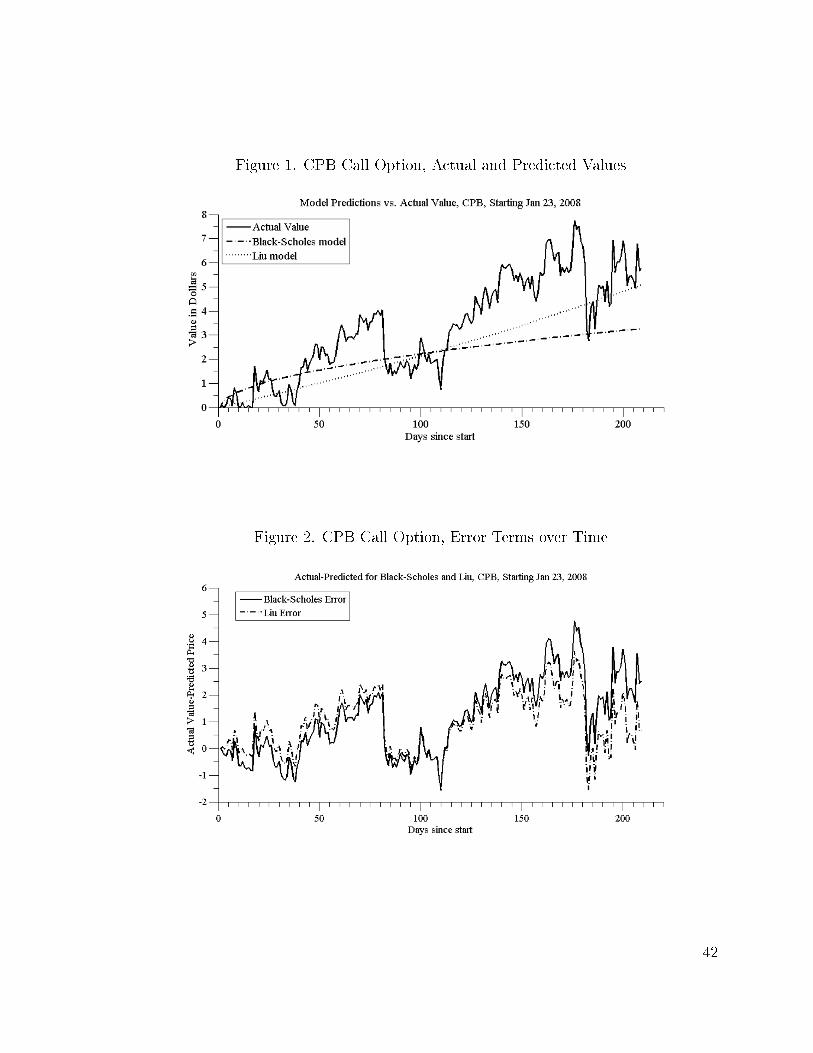
Figure 1. CPB Call Option, Actual and Predicted Values
Figure 2. CPB Call Option, Error Terms over Time
42

5.2 Data for Each Trial
Here we report the data from each individual trial (30, 60, 90, 120, 150, 180, 210
and 240 days, respectively), including the "BS-Liu" term, which denotes the extent
to which Liu outperformed Black-Scholes if positive, and vice versa if negative.
30 Day Trial
Table 3. ARMSE for 30 Day Trial
Strike BS ARMSE Liu ARMSE BS-Liu pT ps
Price0 − 1 1.92486 1.67162 .25323 1.52793E-08 8.00E-06
Price0 1.71410 1.56573 .14834 .001143 0.2914
Price0 + 1 1.6896 1.60751 .08210 .030167 0.03016736
Table 4. AMAE for 30 Day Trial
Strike BS AMAE Liu AMAE BS-Liu pT ps
Price0 − 1 1.76327 1.50026 .26301 9.65095E-10 1.30E-07
Price0 1.50726 1.31171 .19555 .1.87E-5 0.0118
Price0 + 1 1.46332 1.31489 .14842 .000288 0.0002879
43

The Liu model outperforms Black-Scholes over all strikes and both measures of
error. This dierence is lower (and less signicant) at the higher strike price.
60 Day Trial
Table 5. ARMSE for 60 Day Trial
Strike BS ARMSE Liu ARMSE BS-Liu pT ps
Price0 − 1 2.56435 2.25535 .28916 6E-09 3.37E-08
Price0 2.38238 2.16196 .19699 5.81E-05 9.11103E-06
Price0 + 1 2.33658 2.18659 .12535 .003025 0.4889
Table 6. AMAE for 60 Day Trial
Strike BS AMAE Liu AMAE BS-Liu pT ps
Price0 − 1 2.31568 1.98591 .30964 4.09E-10 1.01E-10
Price0 2.09504 1.82020 .25128 8.65E-07 2.5894E-08
Price0 + 1 2.02845 1.80423 .19997 2.31E-05 0.0053
We again see Liu outperforming Black-Scholes, with a decreasing performance as
strike increases. However, the dierences are of a slightly greater magnitude than
those from the 30 day trial.
44

90 Day Trial
Table 7. ARMSE for 90 Day Trial
Strike BS ARMSE Liu ARMSE BS-Liu pT ps
Price0 − 1 2.95889 2.75404 .20485 2.06E-08 2.83E-06
Price0 2.80372 2.68368 .12005 .00111 0.0606
Price0 + 1 2.76366 2.71021 .05346 .07779 0.9745
Table 8. AMAE for 90 Day Trial
Strike BS AMAE Liu AMAE BS-Liu pT ps
Price0 − 1 2.63206 2.39631 .23575 5.07E-10 3.35E-08
Price0 2.44470 2.26261 .18209 5.22E-06 4.90E-04
Price0 + 1 2.38414 2.24866 .13548 .00031 0.0208
Liu again outperforms Black-Scholes, with results very similar to those from the
30 day trial.
45

120 Day Trial
Table 9. ARMSE for 120 Day Trial
Strike BS ARMSE Liu ARMSE BS-Liu pT ps
Price0 − 1 3.46909 3.27759 .191501 2.28E-10 3.96E-08
Price0 3.31661 3.19266 .12395 5.83567E-05 0.004
Price0 + 1 3.25896 3.18850 .07046 .01188 0.2146
Table 10. AMAE for 120 Day Trial
Strike BS AMAE Liu AMAE BS-Liu pT ps
Price0 − 1 3.08833 2.83781 .25052 9.13E-13 1.66E-10
Price0 2.905288 2.69522 .210064 1.74E-08 1.94E-06
Price0 + 1 2.82790 2.65580 .17211 1.83E-06 2.62E-04
46

150 Day Trial
Table 11. ARMSE for 150 Day Trial
Strike BS ARMSE Liu ARMSE BS-Liu pT ps
Price0 − 1 3.9225 3.8284 .09410 0.00014 7.81E-04
Price0 3.7970 3.75662 0.04037 .06828 0.3584
Price0 + 1 3.74651 3.74665 -0.00014 .49783 0.5589
Table 12. AMAE for 150 Day Trial
Strike BS AMAE Liu AMAE BS-Liu pT ps
Price0 − 1 3.4860 3.3063 .17970 1.22E-10 5.67E-08
Price0 3.32953 3.18051 .14903 8.12E-07 1.17E-04
Price0 + 1 3.25826 3.13904 .11922 4.23E-05 0.0044
By this point, we have seen the BS −Liu values dipping back towards 0 for both
RMSE and MAE. As we will see, this trend continues as our time periods grow. It is
also worth noting that the BSRMSE −LiuRMSE decrease began at the 120-day point,
whereas this decrease didn't occur until the 150-day trials for BSMAE−LiuMAE. We
speculate that this is due to RMSE's higher sensitivity to large errors, which occur
47

with greater frequency at later times (a forecast for 30 days in the future will usually
be more accurate than one looking 150 days out).
180 Day Trial
Table 13. ARMSE for 180 Day Trial
Strike BS ARMSE Liu ARMSE BS-Liu pT ps
Price0 − 1 4.23541 4.34606 -0.11064 .00754 0.4718
Price0 4.09850 4.24894 -0.15045 .000402 5.54E-04
Price0 + 1 4.03509 4.21470 -0.17958 2.52E-05 1.93E-07
Table 14. AMAE for 180 Day Trial
Strike BS AMAE Liu AMAE BS-Liu pT ps
Price0 − 1 3.76579 3.73047 .03531 .101204 0.002
Price0 3.60026 3.58468 .015581 .28848 0.136
Price0 + 1 3.51812 3.52289 -0.00477 .43058 0.7166
48
210 Day Trial
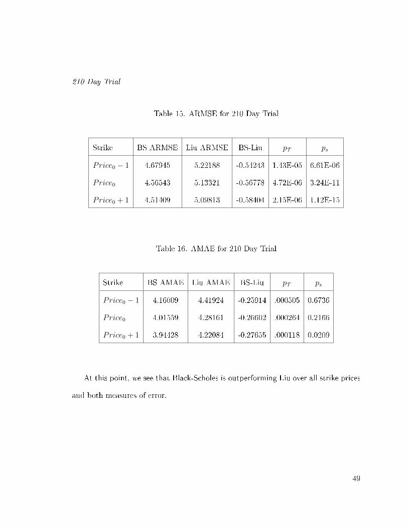
Table 15. ARMSE for 210 Day Trial
Strike BS ARMSE Liu ARMSE BS-Liu pT ps
Price0 − 1 4.67945 5.22188 -0.54243 1.43E-05 6.61E-06
Price0 4.56543 5.13321 -0.56778 4.72E-06 3.24E-11
Price0 + 1 4.51409 5.09813 -0.58404 2.15E-06 1.12E-15
Table 16. AMAE for 210 Day Trial
Strike BS AMAE Liu AMAE BS-Liu pT ps
Price0 − 1 4.16009 4.41924 -0.25914 .000505 0.6736
Price0 4.01559 4.28161 -0.26602 .000264 0.2166
Price0 + 1 3.94428 4.22084 -0.27655 .000118 0.0209
At this point, we see that Black-Scholes is outperforming Liu over all strike prices
and both measures of error.
49

240 Day Trial
Table 17. ARMSE for 240 Day Trial
Strike BS ARMSE Liu ARMSE BS-Liu pT ps
Price0 − 1 4.88025 5.54879 -0.66854 1.35E-06 4.89E-13
Price0 4.75448 5.43733 -0.68285 6.71E-07 8.03E-16
Price0 + 1 4.69039 5.37933 -0.68895 4.59E-07 3.78E-17
Table 18. AMAE for 240 Day Trial
Strike BS AMAE Liu AMAE BS-Liu pT ps
Price0 − 1 4.33682 4.70318 -0.36636 2.6E-05 8.24E-06
Price0 4.18421 4.54965 -0.36544 1.85E-05 1.93E-07
Price0 + 1 4.10179 4.46923 -0.36743 1.28E-05 6.25E-09
5.3 Discussion
Performance over Short Time Periods
Perhaps the most striking result of the data analysis is the extent to which the
Liu model consistently outperforms the Black-Scholes model over short time periods.
While Black-Scholes is certainly not the most sophisticated or accurate model for
50

option prices in use today, it is it's similarity to the Liu model which is of particular
interest. Both models assume that option prices are aected only by the risk-free
interest rate and a constant volatility, with the interest-rate creating a deterministic
movement and the volatility acting on an uncertain process. And in both cases, that
uncertain process behaves according to a distribution which takes mean and vari-
ance as parameters and maximizes entropy within the respective measure. By design,
the only dierence between the two models is that the Black-Scholes model uses the
probability measure, whereas the Liu model is based on the credibility measure. For
this reason, we believe the most useful and promising outcome of this research is
in investigating whether more sophisticated probability models might be improved
by assuming a fuzzy process instead. For example, a model developed by Heston [6]
assumes that volatility, instead of remaining constant, behaves according to a stochas-
tic process as a function of both current and long-term mean volatility. In terms of
the previously mentioned stochastic dierential equation (2.1), Heston theorized that
volatility could be modeled by the equation:
dvt = φ(ω − vt)dt+ ε√vtdBt (V.1)
where vt is volatility at time t, ω is the long-term mean volatility, φ is the rate at
which volatility tends to revert to that mean, and ε is the volatility of the process
used to determine volatility of the stock. It's possible, based on the results of this
study, that volatility might be more accurately modeled (at least under certain cir-
cumstances) replacing the Brownian movement (dBt) with a Liu process. Another
51

popular model, called GARCH (generalized auto-regressive conditional heteroskedac-
ity), assumes variance to vary according to vt rather than it's root [4]:
dvt = φ(ω − vt)dt+ εvtdBt (V.2)
Here we see another opportunity to investigate the possibility that replacing the
Brownian process with a fuzzy process might yield more accurate forecasts.
Performance over Longer Time Periods
As the time periods got longer, the Liu model's accuracy began to deteriorate, with
Black-Scholes outperforming Liu signicantly at times over 180 days. This indicates
both a potential limitation on the applicability of fuzzy processes, as well as possible
evidence of a aw in the overall rationale for using this type of process to model
nancial behavior. The Liu error terms tend to increase exponentially as the time
period increases past 180 days.
Other Relationships
Another direction for future research is an investigation of the relationship be-
tween model performance and variables other than time, such as interest rate and the
dierence between current price and strike price (referred to as the "moneyness" of the
option - i.e. the extent to which it is "in-the-money" or "out-of-the-money"). While
the options in my research do vary in interest rate and moneyness in order to provide
more robust overall results, the particular relationships between these variables and
overall accuracy was not closely analyzed.
52

The other major question that arises is "WHY does the Liu model behave the way
it does?" By looking at Figure 4 (3) we can compare the distributions of normally
distributed fuzzy and random variables (both random and fuzzy variables are "stan-
dardized" with mean= 0 and standard deviation/diusion= 1). We see that the fuzzy
distribution places less weight on values close to the mean, which could contribute to
the dierence in performance we see between the two.
Figure 3. Normal Fuzzy vs. Normal Random
We feel that a deeper analysis of this property, as well as the fact that the credibil-
ity measure averages two dierent values for a particular set (both possibility (III.1)
and necessity (III.2)), might yield insight into the dierences in behavior between
random and fuzzy processes.
53

CHAPTER VI
CONCLUSION
In this thesis, we have provided a review of existing literature on continuous-
time stochastic processes and their application in creating the Black-Scholes formula
for pricing European call options. Likewise, we have compiled information on fuzzy
processes into a stand-alone, axiomatic foundation for Liu's fuzzy model for option
prices. This provides not only insight into the model, but also a comparison of the
fundamental similarities and dierences between fuzzy and stochastic continuous-
time processes. We then performed a comparison between the actual results of these
two models using recent historical stock data. While the average error terms of both
models are signicantly larger than those produced by more sophisticated models, the
Liu model tended to outperform Black-Scholes over shorter time intervals. Though
this does not suggest the Liu model as a replacement for more modern techniques,
it is signicant in that the primary dierence between the two models is the use of
a stochastic vs. fuzzy continuous-time process. Since many modern models are built
on stochastic processes, it seems promising to consider adapting some of these models
to fuzzy processes as well.
54

REFERENCES
[1] F. Black and P. Karasinski, Bond and option pricing when short rates are log-normal, Financial Analysts Journal (1991), 5259.
[2] F. Black and M. Scholes, The pricing of options and corporate liabilities, TheJournal of Political Economy (1973), 637654.
[3] V. Capasso and D. Bakstein, An introduction to continuous-time stochasticprocesses: theory, models, and applications to nance, biology, and medicine,Birkhauser, 2005.
[4] P.H.B.F. Franses and D.J.C. Dijk, Forecasting stock market volatility using (non-linear) garch models, Journal of Forecasting (1996), 229235.
[5] J. Gao and X. Gao, A new stock model for credibilistic option pricing, Journalof Uncertain Systems 2 (2008), no. 4, 243247.
[6] S.L. Heston, A closed-form solution for options with stochastic volatility withapplications to bond and currency options, Review of nancial studies 6 (1993),no. 2, 327.
[7] C.C. Hsia, On binomial option pricing, The Journal of Financial Research 6
(1983), no. 1, 4146.
[8] J. Hull and A. White, The pricing of options on assets with stochastic volatilities,Journal of nance (1987), 281300.
[9] ET Jaynes, Information theory and statistical mechanics, Physical Review 106
(1957), no. 4, 620630.
[10] H.H. Kuo, Introduction to stochastic integration, Springer Verlag, 2006.
[11] Steve Lalley, Lecture 6: The ito calculus, 2001, 2001, University ofChicago Lecture Notes, available at http://galton.uchicago.edu/ lalley/Cours-es/390/Lecture6.pdf.
[12] P. Li and B. Liu, Entropy of credibility distributions for fuzzy variables, FuzzySystems, IEEE Transactions on 16 (2008), no. 1, 123129.
55

[13] X. Li and B. Liu, New independence denition of fuzzy random variable andrandom fuzzy variable, World Journal of Modelling and Simulation 2 (2006),no. 5, 338342.
[14] , A sucient and necessary condition for credibility measures, World 14(2006), no. 5, 527535.
[15] X. LI and B. LIU, Maximum entropy principle for fuzzy variables, Int. J. Unc.Fuzz. Knowl. Based Syst. 15 (2007), no. supp02, 4352.
[16] B. Liu, A survey of credibility theory, Fuzzy Optimization and Decision Making5 (2006), no. 4, 387408.
[17] , Fuzzy process, hybrid process and uncertain process, Journal of UncertainSystems 2 (2008), no. 1, 316.
[18] B. Liu and Y.K. Liu, Expected value of fuzzy variable and fuzzy expected valuemodels, Fuzzy Systems, IEEE Transactions on 10 (2002), no. 4, 445450.
[19] R.L. McDonald, Derivatives markets, 2006, New York: Pearson Education.
[20] Z. Qin and X. Li, Fuzzy calculus for nance, (2008).
[21] R. Rudin, Real and complex analysis, New York. Mc-Graw-Hill (1974).
[22] C.E. Shannon and W. Weaver, The mathematical theory of communication, Cite-seer, 1959.
[23] S. Stoyanov, S. Rachev, and F. Fabozzi, Probability metrics with applications innance, Journal of Statistical Theory and Practice (2007), 253277.
[24] D.W. Stroock, Probability theory: an analytic view, Cambridge Univ Pr, 2010.
[25] J. Van Campenhout and T. Cover,Maximum entropy and conditional probability,Information Theory, IEEE Transactions on 27 (1981), no. 4, 483489.
[26] D. Wang, Estimation of the hidden parameters for the distribution of special fuzzyrandom variables, Journal of Statistical Theory and Practice (2010), 337334.
[27] Z. Wang and F. Tian, A note of the expected value and variance of fuzzy variables,International Journal of Nonlinear Science 9 (2010), no. 4, 486492.
[28] J.B. Wiggins, Option values under stochastic volatility: Theory and empiricalestimates* 1, Journal of nancial economics 19 (1987), no. 2, 351372.
[29] L.A. Zadeh, Fuzzy sets as a basis for a theory of possibility* 1, Fuzzy sets andsystems 1 (1978), no. 1, 328.
56

APPENDIX A
MATLAB CODE
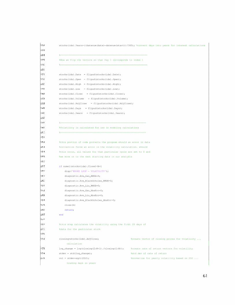
Single Iteration
The rst program listed does the computations for a single starting date over a
given list of stocks. As parameters, it takes a starting date, the length of the period,
the interest rate on the starting date, a "reversion" parameter for the Gao model
(which was not included in the results), and a single stock or list of stocks.
57

1 function [stocks, diagnostic] = date_offset(start, date_offset, strike_offset, reversion, interest_rate, varargin)
2 %%THE PROGRAM IS ORGANIZED INTO FIVE STEPS AS FOLLOWS:
3 %
4 %STEP 1 − BRING IN THE NECESSARY STOCK DATA FOR THE SPECIFIED STARTING DATE
5 %AND TIME PERIOD FOR ALL STOCKS IN LIST
6 %Data is brought in using the Yahoo Historical Stock Database and MATLAB's
7 %urlread command.
8 %
9 %STEP 2 − CALCULATE MODEL PRICES FOR HYPOTHETICAL OPTIONS EXPIRING ON DAY 1, 2,
10 %.., N FOR EACH STOCK
11 %The first part of this step is to estimate the volatility of each stock
12 %using the first 20 days of the time period under consideration. Volatility
13 %is defined as the standard deviation of the rate of return over this
14 %period.
15 %Once we have volatility, we use volatility, interest rate, current price
16 %and strike price to estimate option values using the Liu and Black−Scholes
17 %models.
18 %
19 %STEP 3 − CALCULATE ACTUAL VALUE OF THESE HYPOTHETICAL OPTIONS
20 %The value of any given option at time T is simply max[e^(−rT)*(Price −
21 %Strike), 0]. The actual value for these options is calculated for days 1,
22 %2, ... , N.
23
24 %STEP 4 − CALCULATE ERROR TERMS (ROOT MEAN SQUARED ERROR (RMSE) AND MEAN ABSOLUTE ERROR (MAE)
25 %FOR EACH STOCK
26
27 %STEP 5 − AVERAGE THESE ERROR TERMS FOR THE WHOLE LIST OF STOCKS
28
29 function f=gao_call(price,strike,rate, time,volatility,drift,reversion,level)
30 Q=(sqrt(6)*pi.*(1−exp(−reversion.*time)))/(pi.*reversion);
31 P=strike−level−((exp(−reversion.*time))*(price−level));
32 f=exp(−rate*time)*(Q*log(1+exp(P/Q))−P);
33
34
35 %This function outputs the price of a European Call using Gao's Fuzzy Mean Reversion Model
36 %Inputs are similar to Liu/Black Scholes, but constant, linear "drift" has been replaced by a rate of reversion ...
and a "level" to which the price tends to revert
37 %Q and P variables are simply used for simplicity
38 end
39
40 function f=liu_call(price, strike, rate, time, volatility, drift)
41 y=@(x) price*exp(−rate.*time)./(1+exp((log(x)−drift*time)*(pi/(sqrt(6)*volatility*time))));
42 f=quad(y,strike/price,100);
43
44 %Function outputs price of a European Call based on Liu's model
58

45 %second line states function for the expected value of a Call with the given parameters
46 %third line integrates function from lower bound of (strike/price) to upper bound of positive infinity ...
(although a real number is used to approximate)
47 end
48
49 stocks = struct([]); %initialize data structure
50 diagnostic=struct('Gao_RMSE', 0, 'BlackScholes_RMSE', 0, 'Liu_RMSE', 0, 'Gao_AbsErr', 0, ...
'BlackScholes_AbsErr', 0, 'Liu_AbsErr', 0, 'Ave_Gao_RMSE', 0, 'Ave_BlackScholes_RMSE', 0, ...
'Ave_Liu_RMSE', 0, 'StDev_Gao_RMSE', 0, 'StDev_BlackScholes_RMSE', 0, 'StDev_Liu_RMSE', 0, ...
'Ave_Gao_AbsErr', 0, 'Ave_BlackScholes_AbsErr', 0, 'Ave_Liu_AbsErr', 0, 'Gao_Over_Percentage', 0, ...
'BS_Over_Percentage', 0, 'Liu_Over_Percentage', 0); %initialize diagnostic structure
51 N=20; %counter for iterations in volatility calculation
52 OFFSET=strike_offset; %fix strike offset based on input parameters
53 RATE=interest_rate; %fix interest rate based on input parameters
54 REVERSION=reversion; %rate of reversion for Gao mean−reversion
55
56 %%INITIALIZE DATES
57 %For the starting date, we convert the date string into date vector format,
58 %then isolate the beginning day (bd), beginning month (bm) and beginning
59 %year (by) so that they can be input using the url for the stock data.
60
61 start_D=datevec(start);
62 bd=num2str(start_D(3));
63 bm=num2str(start_D(2)−1);
64 by=num2str(start_D(1));
65
66 %Ending date is calculated as the beginning date plus the number of days
67 %specified for the length of the time period. The date is broken apart into
68 %ending day (ed), ending month (em) and ending year (ey) similar to the
69 %beginning date.
70
71 end_date=datenum(start_D)+date_offset;
72 end_D=datevec(end_date);
73 ed=num2str(end_D(3));
74 em=num2str(end_D(2)−1);
75 ey=num2str(end_D(1));
76
77
78 % this portion of code is used to determine if a frequency of data
79 % reporting was requested other than "daily" − since my analysis uses daily
80 % value, this is not changed throughout
81
82 temp = find(strcmp(varargin,'frequency') == 1); % search for frequency
83 if isempty(temp) % if not given
84 freq = 'd'; % default is daily
85 else % if user supplies frequency
59

86 freq = varargintemp+1; % assign to user input
87 varargin(temp:temp+1) = []; % remove from varargin
88 end
89 clear temp
90
91 %here we determine the type of input used to specifiy the stock(s) to be
92 %analyzed. for the purposes of this analysis, a .txt file containing a list
93 %of ticker symbols is used
94
95 if isempty(strfind(varargin1,'.txt')) % If individual tickers
96 tickers = varargin; % obtain ticker symbols
97 else % If text file supplied
98 tickers = textread(varargin1,'%s'); % obtain ticker symbols
99 end
100
101 h = waitbar(0, 'Please Wait...'); % create waitbar
102 idx = 1; % idx for current stock data
103
104 % cycle through each ticker symbol and retrieve historical data
105 for i = 1:length(tickers)
106
107 % update waitbar to display current ticker
108 waitbar((i−1)/length(tickers),h,sprintf('%s %s %s%0.2f%s', ...
109 'Retrieving stock data for',tickersi,'(',(i−1)*100/length(tickers),'%)'))
110
111 % download historical data using the Yahoo! Finance website
112 [temp, status] = urlread(strcat('http://ichart.finance.yahoo.com/table.csv?s='...
113 ,tickersi,'&a=',bm,'&b=',bd,'&c=',by,'&d=',em,'&e=',ed,'&f=',...
114 ey,'&g=',freq,'&ignore=.csv'));
115
116 if status
117 % organize data by using the comma delimiter
118 [date, op, high, low, cl, volume, adj_close] = ...
119 strread(temp(43:end),'%s%s%s%s%s%s%s','delimiter',',');
120
121
122 stocks(idx).Ticker = tickersi; % obtain ticker symbol
123 stocks(idx).Date = date; % save date data
124 %disp(date);
125 stocks(idx).Open = str2double(op); % save opening price data
126 stocks(idx).High = str2double(high); % save high price data
127 stocks(idx).Low = str2double(low); % save low price data
128 stocks(idx).Close = str2double(cl); % save closing price data
129 stocks(idx).Volume = str2double(volume); % save volume data
130 stocks(idx).AdjClose = str2double(adj_close); % save adjustied close data
131 stocks(idx).Days=(datenum(date)−datenum(start)); %converted dates into days since start
60
132 stocks(idx).Years=((datenum(date)−datenum(start))/365); %convert days into years for interest calculations
133
134 %===============================================================
135 %Now we flip the vectors so that Day 1 corresponds to index 1
136 %===============================================================
137
138 stocks(idx).Date = flipud(stocks(idx).Date);
139 stocks(idx).Open = flipud(stocks(idx).Open);
140 stocks(idx).High = flipud(stocks(idx).High);
141 stocks(idx).Low = flipud(stocks(idx).Low);
142 stocks(idx).Close = flipud(stocks(idx).Close);
143 stocks(idx).Volume = flipud(stocks(idx).Volume);
144 stocks(idx).AdjClose = flipud(stocks(idx).AdjClose);
145 stocks(idx).Days = flipud(stocks(idx).Days);
146 stocks(idx).Years = flipud(stocks(idx).Years);
147
148 %==============================================================
149 %Volatility is calculated for use in modeling calculations
150 %==============================================================
151
152 %this portion of code protects the program should an error in data
153 %collection force an error in the volatility calculation. should
154 %this occur, all values for that particular cycle are set to 0 and
155 %we move on to the next starting date in our analysis
156
157 if numel(stocks(idx).Close)<N+1
158 disp('BROKE LOOP − VOLATILITY');
159 diagnostic.Ave_Gao_RMSE=0;
160 diagnostic.Ave_BlackScholes_RMSE=0;
161 diagnostic.Ave_Liu_RMSE=0;
162 diagnostic.Ave_Gao_AbsErr=0;
163 diagnostic.Ave_Liu_AbsErr=0;
164 diagnostic.Ave_BlackScholes_AbsErr=0;
165 close(h)
166 return;
167 end
168
169 %this step calculates the volatility using the first 20 days of
170 %data for the particular stock
171
172 closing=stocks(idx).AdjClose; %create vector of closing prices for volatility ...
calculation
173 log_change = log(closing(2:N+1)./closing(1:N)); %create rate of return vectors for volatility
174 stdev = std(log_change); %std dev of rate of return
175 vol = stdev*sqrt(252); %normalize for yearly volatility based on 252 ...
trading days in years
61
176 stocks(idx).Volatility=vol; %save volatility in stock structure
177 idx = idx + 1; % increment stock index
178
179 clear log_change stdev vol
180 end
181 % clear variables made in for loop for next iteration
182 clear date op high low cl volume adj_close temp status
183
184
185 % update waitbar
186 waitbar(i/length(tickers),h)
187 end
188
189 %========================================================================
190 %Now we calculate predicted values of options, using a loop to cycle
191 %through stock tickers, then an inner loop that cycles through days,
192 %pricing options for each day
193 %=======================================================================
194
195 k=1;
196 l=numel(stocks(k).Days);
197 s=length(tickers)+1;
198 while k < s
199 j=1; %initialize counter for number of days in period
200 PRICE=stocks(k).AdjClose(1); %set the stock's price to the price on day 1
201 STRIKE=PRICE + OFFSET; %set the option's strike price based on user input
202 VOLATILITY=stocks(k).Volatility; %retrieve stock's volatility from data structure
203 l=numel(stocks(k).Years);
204
205 %the "over" counters are used to keep track of times that the model
206 %over−priced an option
207
208 LIU_OVER=0;
209 GAO_OVER=0;
210 BS_OVER=0;
211 while j < l
212
213 %prices are calculated for an option expiring on day(j)
214
215 [call, put]=blsprice(PRICE, STRIKE, RATE, stocks(k).Years(j), VOLATILITY, 0);
216 liu=liu_call(PRICE, STRIKE, RATE, stocks(k).Years(j), VOLATILITY, RATE);
217 gao=gao_call(PRICE, STRIKE, RATE, stocks(k).Years(j), VOLATILITY, RATE, REVERSION, PRICE);
218
219 %actual value of option, had it been purchased, is calculated
220
221 actual=(exp(−.06*stocks(k).Years(j)))*(stocks(k).AdjClose(j)−stocks(k).AdjClose(1));
62

222 if actual>0
223 stocks(k).Actual(j)=actual;
224 else
225 actual=0;
226 stocks(k).Actual(j)=actual;
227 end
228
229 %temporary values are stored in data structure
230
231 stocks(k).BlackScholes(j)=call;
232 stocks(k).Liu(j)=liu;
233 stocks(k).Gao(j)=gao;
234 stocks(k).BlackScholes_Error(j)=actual−call;
235 stocks(k).Liu_Error(j)=actual−liu;
236 stocks(k).Gao_Error(j)=actual−gao;
237 stocks(k).BlackScholes_AbsError(j)=abs(actual−call);
238 stocks(k).Liu_AbsError(j)=abs(actual−liu);
239 stocks(k).Gao_AbsError(j)=abs(actual−gao);
240 if (actual−call)<0
241 BS_OVER=BS_OVER+1;
242 end
243 if (actual−liu)<0
244 LIU_OVER=LIU_OVER+1;
245 end
246 if (actual−gao)<0
247 GAO_OVER=GAO_OVER+1;
248 end
249 j=j+1;
250 end
251
252 stocks(k).Gao(1)=0; %otherwise the price on day 0 (which should be 0) returns NaN
253 stocks(k).Gao_Error(1)=0; %prevents NaN values in Error, RMSE
254
255 %===============================================================
256 %Here we calculate the Root Mean Squared Error for each model
257 %−This is done by summing the square of each day's error term, then
258 %−taking an average, and then the square root of this average.
259 %==============================================================
260
261 BS_sum=sum((stocks(k).BlackScholes_Error).^2)/numel(stocks(k).Days);
262 BS_root=sqrt(BS_sum);
263 stocks(k).BlackScholes_RMSE=BS_root;
264 diagnostic.BlackScholes_RMSE(k)=BS_root;
265 L_sum=sum((stocks(k).Liu_Error).^2)/numel(stocks(k).Days);
266 L_root=sqrt(L_sum);
267 stocks(k).Liu_RMSE=L_root;
63

268 diagnostic.Liu_RMSE(k)=L_root;
269 G_sum=sum((stocks(k).Gao_Error).^2)/numel(stocks(k).Days);
270 G_root=sqrt(G_sum);
271 stocks(k).Gao_RMSE=G_root;
272 diagnostic.Gao_RMSE(k)=G_root;
273 diagnostic.Liu_Over_Percentage(k)=LIU_OVER/numel(stocks(k).Days);
274 diagnostic.Gao_Over_Percentage(k)=GAO_OVER/numel(stocks(k).Days);
275 diagnostic.BS_Over_Percentage(k)=BS_OVER/numel(stocks(k).Days);
276
277
278 stocks(k).Gao(1)=0; %otherwise the price on day 0 (which should be 0) returns NaN
279 stocks(k).Gao_Error(1)=0; %prevents NaN values in Error, RMSE
280
281 %=================================================================
282 %Now we calculate Mean Absolute Error for each model
283 %=================================================================
284
285 diagnostic.Gao_AbsErr(k)=mean(stocks(k).Gao_AbsError);
286 diagnostic.Liu_AbsErr(k)=mean(stocks(k).Liu_AbsError);
287 diagnostic.BlackScholes_AbsErr(k)=mean(stocks(k).BlackScholes_AbsError);
288
289
290
291 %these counters keep track of the model with lowest RMSE for each
292 %stock
293
294 if (G_root < BS_root) && (G_root < L_root)
295 stocks(k).Winner='GAO!';
296 end
297
298 if (L_root < BS_root) && (L_root < G_root)
299 stocks(k).Winner='Liu!';
300 end
301
302 if (BS_root < L_root) && (BS_root < G_root)
303 stocks(k).Winner='Black−Scholes';
304 end
305 k=k+1;
306 end
307
308 %=========================================================================
309 %Now we take an average (and standard deviation) of the RMSE and MAE over
310 %all stocks and store it in the diagnostic data structure for use in
311 %analysis
312 %==========================================================================
313 diagnostic.Ave_Gao_RMSE=mean(diagnostic.Gao_RMSE);
64

314 diagnostic.Ave_BlackScholes_RMSE=mean(diagnostic.BlackScholes_RMSE);
315 diagnostic.Ave_Liu_RMSE=mean(diagnostic.Liu_RMSE);
316 diagnostic.StDev_Gao_RMSE=std(diagnostic.Gao_RMSE);
317 diagnostic.StDev_Liu_RMSE=std(diagnostic.Liu_RMSE);
318 diagnostic.StDev_BlackScholes_RMSE=std(diagnostic.BlackScholes_RMSE);
319 diagnostic.Ave_Gao_AbsErr=mean(diagnostic.Gao_AbsErr);
320 diagnostic.Ave_Liu_AbsErr=mean(diagnostic.Liu_AbsErr);
321 diagnostic.Ave_BlackScholes_AbsErr=mean(diagnostic.BlackScholes_AbsErr);
322
323 diagnostic.Ave_Liu_Over_Percentage=mean(diagnostic.Liu_Over_Percentage);
324 diagnostic.Ave_Gao_Over_Percentage=mean(diagnostic.Gao_Over_Percentage);
325 diagnostic.Ave_BS_Over_Percentage=mean(diagnostic.BS_Over_Percentage);
326
327 close(h) % close waitbar
328 end
65

Aggregated Data over Multiple Iterations
The second program is used for running multiple 30 day trials at dierent (ran-
domized) starting dates. It takes only the number of trials as a parameter, produces
N random starting dates within the time-frame specied, runs the "date oset" pro-
gram for each one, and then aggregates the information and outputs it to an Excel
spreadsheet for analysis. Modications of this were used for trials of dierent lengths.
66

1 function [M30, DATA_30, INTEREST] = MACRO_30(numtrials)
2
3 %%BRINGING IN INTEREST RATE DATA
4 %Data is read from an excel file, and stored in a vector indexed with the
5 %first cell containing the interest rate from "Day 1" of our analysis
6
7 int_rate_vector =xlsread('interest_rate_2008_2012.xlsx');
8 INTEREST=int_rate_vector;
9
10 %%RANDOMIZING DATES
11 %Using their MATLAB serial numbers, I randomly select n "dates" (integers
12 %in the correct range of serial numbers) from which to use as starting
13 %points of my test periods.
14 n=numtrials;
15 date=randi([733409,734720],1,n);
16
17 %%OTHER INPUTS
18 %The number of trials is taken as a parameter of the function, while the
19 %strike offset vector is (currently) a fixed vector running from −1 to 1.
20 strike=[−1:1];
21
22 %%THE LOOP
23 %The goal is run my model analysis function n times for each strike price,
24 %and then write this data to an excel workbook, with a seperate worksheet
25 %for each strike price.
26 for k=1:numel(strike)
27 for i=1:n
28 activeDate=date(i);
29 dateTest=date(i);
30 if weekday(dateTest) == 7 %Here I'm making sure that I don't start on a Saturday ...
(7) or Sunday (1)
31 activeDate=activeDate+2; %for my interest rate calculation by moving the ...
starting date off
32 end %the weekends
33 if weekday(dateTest) == 1
34 activeDate=activeDate+1;
35 end
36
37 int_rate_date=(activeDate−733408); %My interest rate data has data point 1 set to ...
January 2, 2008
38
39 while int_rate_vector(int_rate_date)> 998 %Since interest rate data is not available on ...
weekends/market holidays
40 int_rate_date=int_rate_date+1; %their value in the vector is NaN. All NaN's were ...
converted to the number
67
41 end %999 so that I can bump the date up a day when I land ...
on these.
42 temp_rate=int_rate_vector(int_rate_date)/100;
43 [STOCKS, SUMMARY]=date_offset(activeDate, 30, strike(k), .1,temp_rate, 'SP100.txt'); %stock loop is run ...
for each strike
44
45 %%DATA STORAGE
46 %Data from each iteration of the stock loop is stored in the
47 %DATA_30 structure
48
49 DATA_30(k).BS_RMSE(i)=SUMMARY.Ave_BlackScholes_RMSE;
50 DATA_30(k).Liu_RMSE(i)=SUMMARY.Ave_Liu_RMSE;
51 DATA_30(k).BS_MAE(i)=SUMMARY.Ave_BlackScholes_AbsErr;
52 DATA_30(k).Liu_MAE(i)=SUMMARY.Ave_Liu_AbsErr;
53 end
54
55 %Now that I have done all the calculations for this strike, I'd
56 %like to store all this data on a worksheet labeled with that
57 %particular strike.
58
59 strikestr=num2str(strike(k));
60 sheetname = genvarname(strikestr);
61 xlswrite('30_day_data', rot90(DATA_30(k).BS_RMSE,3), sheetname, 'A2');
62 xlswrite('30_day_data', rot90(DATA_30(k).Liu_RMSE,3), sheetname, 'B2');
63 xlswrite('30_day_data', rot90(DATA_30(k).BS_MAE,3), sheetname, 'C2');
64 xlswrite('30_day_data', rot90(DATA_30(k).Liu_MAE,3), sheetname, 'D2');
65
66 end
68

APPENDIX B
GLOSSARY
69

GLOSSARY
call option An option to buy a stock, on a specied date, at a specied price. Put
options have value when the true price is higher than the strike price at maturity.
1, 11, 34
continuously-compounded interest Normal compound interest re-invests inter-
est earned during each compounding period, so that interest may be earned
on it during the next period. Continuously-compounded interest occurs in the
special case where the compounding period becomes innitesimally small. 9
expiration date For a European option, the expiration date is the date on which
the option can be exercised. 8, 34
grade of membership The "grade of membership" represents our belief that a cer-
tain event or outcome is possible. 14
in-the-money An option that is "in-the-money" can be exercised for a net gain.
For a call option, this means that the spot price is greater than the strike price,
and vice versa for a put option. 8, 40
out-of-the-money An option that is "out-of-the-money" can not be exercised for
a net gain, and is thus not exercised. An "out-of-the-money" option is worth
nothing. 8, 40
70

put option An option to sell a stock, on a specied date, at a specied price. Put
options have value when the true price is lower than the strike price at maturity.
1
spot price The price of an option's underlying stock on the date of expiration. 8,
13
strike price The price listed on an option, at which the underlying asset can be
bought/sold at expiration. 8, 34, 40
synthetic option A synthetic option is a combination of nancial instruments which
has the same payo prole of another instrument. For our purposes, we consider
the special case of synthetic puts and calls, which are created by nancing a
position in the underlying asset through borrowing at the risk-free rate. 9
71