No.07-E-20 August 2007

Price Setting in Japan: Evidence from CPI Micro Data

*Masahiro Higomasahiro.higo@boj.or.jp

**Yumi Saitayumi.saita@boj.or.jp Bank of Japan 2-1-1 Nihonbashi Hongoku-cho, Chuo-ku, Tokyo 103-8660

* Research and Statistics Department **Research and Statistics Department

Papers in the Bank of Japan Working Paper Series are circulated in order to stimulate discussion and comments. Views expressed are those of authors and do not necessarily reflect those of the Bank. If you have any comment or question on the working paper series, please contact each author. When making a copy or reproduction of the content for commercial purposes, please contact the Public Relations Department (webmaster@info.boj.or.jp) at the Bank in advance to request permission. When making a copy or reproduction, the source, Bank of Japan Working Paper Series, should explicitly be credited.

Bank of Japan Working Paper Series

Price Setting in Japan: Evidence from CPI Micro Data

Masahiro Higo* and Yumi Saita†

August, 2007

Abstract

This paper investigates the price-setting behavior in Japan by using the CPI micro data

in the Retail Price Survey from 1989 to 2003. We establish the four facts as follows. First,

the frequency of price changes for goods is high while that for services is low. The

frequency of price changes for goods has increased during the 1990s while that for services

has greatly decreased. Second, many items have a downward sloping hazard function while

some have the flexible-type or the Taylor-type hazard function. Third, in most of the

categories in the CPI, a decline in the frequency of price changes has contributed to the

drop in the CPI inflation rate since the 1990s while the size of price changes has remained

roughly unchanged. Fourth, the heterogeneity in the frequency of price changes across

categories and its evolution are strongly influenced by the differences in the share of labor

costs in the production costs and changes in the firm’s price strategy regarding temporary

sales.

Keyword: Consumer Price Index, Price-setting, Price stickiness, Frequency of price

changes, Hazard functions, Time-dependent pricing, State-dependent pricing

JEL classifications: E31, D40, C41

We would like to thank Ken Ariga, John Leahy, Kazuko Kano and participants at the conference “Economic Development in Japan Since the 1990s”, “Monetary Policy Workshop” and “Inflation Dynamics in Japan, US and EU” for helpful comments and discussions. We also would like to thank Kosuke Aoki, Andrew Levin, Makoto Shimizu and staff members at the Bank of Japan. We are grateful to Statistics Bureau, Ministry of Internal Affairs and Communications for providing us with the data. We are grateful to Kenji Nishizaki, Izumi Takagawa, Koji Nakamura, Chie Arai, Rie Yamaoka, Ayako Kouju, and Sawako Hagiwara for research assistance. The views expressed in this paper are those of the authors and do not necessarily reflect those of the Bank of Japan or the Research and Statistics Department. * Research and Statistics Dept., Bank of Japan; e-mail:masahiro.higo@boj.or.jp † Research and Statistics Dept., Bank of Japan; e-mail:yumi.saita@boj.or.jp

1 1

1. Introduction The nature of price-setting behavior has important implications on a wide range of issues in

macroeconomics. One of the most important issues is that the degree of price stickiness

influences the nature of business cycles. If prices are sticky, prices do not adjust

immediately in response to various shocks. While price stickiness stabilizes the volatility of

prices, it increases the volatility of real output. Sakura, Sasaki and Higo [2005] find that in

Japan, while the real growth rate has been fluctuating since the 1990s, the inflation rate has

remained stable. Price stickiness may be one of the causes for this phenomenon.

Another important issue is that price stickiness distorts resource allocation. When

heterogeneity in price stickiness across individual products exists, relative prices between

sticky-price and flexible-price products change in response to shocks. The change in the

relative prices distorts the resource allocation and entails a social welfare loss. The

magnitude of the social welfare loss depends on the degree of macro price stickiness and

the amount of heterogeneity in the price stickiness across individual products. In addition,

whether price stickiness is time-invariant (time-dependent pricing) or time-variant (e.g.

state-dependent pricing) determines the extent of the loss.

There are two approaches to investigate price-setting behavior. One is to conduct an

interview survey of firms. Blinder et al.[1998] find that in the US there are large differences

in the frequency of price changes among firms or items, and the median firm adjusts prices

about once a year. Bank of Japan [2000] finds, based on a questionnaire survey of 630 firms,

that firms most commonly change prices once or twice a year in Japan.

The other approach is to use micro data underlying the consumer and producer price

indexes. Bils and Klenow[2004] show that the average frequency of price changes for the

US CPI is around 25 percent per month, which is larger than the frequency obtained by the

firms survey. The Eurosystem Inflation Persistence Network investigated price-setting

behavior by using micro data in most of the euro countries. Its findings are as follows. First,

the average frequency of price changes is 15 percent per month. Second, the frequency

varies across products, with very frequent changes for energy products and unprocessed

food, and relatively infrequent changes for non-energy industrial goods and services. Third,

price decreases are not uncommon even when the inflation rate is positive. Fourth, the size

of price changes is 8 to 10 percent, which is much larger than the prevailing inflation rate.

Recently Nakamura and Steinsson [2007] reported interesting stylized facts as follows.

First, when sales are excluded, the average frequency of price changes for the US CPI is

2 2

only between 9 and 11 percent per month, which is almost the same as the frequency given

in the firms’ survey. Second, one third of price changes are price decreases. Third, the

frequency of price increases responds to inflation while the frequency of price decreases

and the size of price changes do not. Fourth, the hazard function of price changes for

individual products is downward sloping for the first few months and then flat. The first,

second and third facts are consistent with a benchmark menu-cost model they propose.

In this paper, we analyze the frequency of price changes, hazard rate of price changes,

survival ratio of prices and the size of price changes using the micro data from the Retail

Price Survey, which is used for compiling Japanese consumer price index. This is the first

attempts in Japan to directly measure price-setting behavior using micro data in Japan.

The paper is organized as follows. In section 2, we explain the characteristics of the

micro data we use and the measurement methodologies. In section 3, we measure the

frequency of price changes to show the heterogeneity in the frequency between goods and

services and across categories, and the development of the frequency since the 1990s. In

section 4, we estimate the hazard rate and the survival ratio of items. In section 5, we

analyze the relationship between the frequency and the size of price changes and the

changes in the CPI inflation. In section 6, we examine the determinants of the price-setting

behavior such as the share of labor costs in the production costs and changes in price

regulations and the firm’s price strategy regarding temporary sales. In section 7, we

summarize our findings.

2. Data and Measurement Methodology (1) Retail Price Survey

We use data set from the Retail Price Survey conducted by the Statistics Bureau, Ministry

of Internal Affairs and Communications. In the Retail Price Survey the Bureau surveys

retail prices of goods and services every month. The CPI is constructed using the price data

in the Retail Price Survey. The Retail Price Survey, therefore, is the most suitable statistics

to analyze the price-setting behavior in Japan’s CPI.

(2) Characteristics of the Data

(i) Selection of Items

We use 493 of 598 CPI items, 372 out of 456 items for goods and 121 out of 142 items for

services; (CY 2000 base)(Chart 1(1)). In this analysis, the following items are excluded

3 3

from our data set.

a. Items whose price data are not used for constructing CPI

b. Items whose price data are partly missing because they are seasonal items

c. Items whose price data are compiled from a large number of prices by each survey city

d. Items whose price data has only short time-series (e.g. only available from January 2002)

For goods, automobiles, personal computers, and seasonal items of textiles, are

excluded. For services, house rent, imputed rent, medical treatment, airplane fares,

telephone charges and mobile telephone charges are excluded (Chart 1(2)).

(ii) Coverage

Our data set covers 68 percent of the CPI total weight. The coverage is high for goods at 84

percent, but low for services at 51 percent (Chart 2). This is because house rent and

imputed rent, which have large shares in the CPI, are excluded. Consequently, the share of

goods is 63 percent in the data set, which is higher than the actual share in the CPI (51

percent).

(iii) Surveyed Prices

In the Retail Price Survey, identical items are surveyed at the outlets in each city. The

Bureau surveys prices of goods and services every month. In addition, temporary price cuts

within seven days are excluded so that the data set is not influenced by short-term sales.

(iv) Number of Samples for Each Item

The data are city averages of individual prices across outlets. Our analysis is based on 55

cities (Chart 3(1))1. We, therefore, have 55 city average price data for each item per month.

For example, a price of an identical refrigerator is surveyed at three outlets in each city.

The Bureau averages three prices and publishes the city average price of the refrigerator.

Thus, data at individual outlet level are not open to public. The number of survey outlets in

each city is around three on average; 2.7 for the CPI total, 2.9 for goods and 2.4 for

services2 (Chart 3(2)).

1 The Bureau surveys prices in 167 cities, towns and villages every month. Among them, 71 city average price data are published. The number of survey outlets varies by item and by city. In particular, the sample size in large cities is sizable compared with that in small cities. We, therefore, exclude the data of 16 major large cities and only use the data of 55 middle-sized cities with a prefectural government or a population of at least 150,000 people. More precisely, according to the changes in the number of survey cities, our data set includes 52 cities for 1989-1993, 54 cities for 1994-1998 and 55 cities for 1999-2003. 2 The number of samples is just one for public services, electricity, gas and water charges and

4 4

(v) Sample Period

This data set contains prices from January 1989 to December 2003. The sample period

starts with the bubble period when the inflation rate was around three percent per year. In

the mid-1990s the inflation rate gradually declined to zero percent and it stayed between

minus one and zero percent after the late 1990s.

(3) Measurement Methodology

We measure four indicators for each item: frequency of price changes, hazard rates,

survival ratios and size of price changes. We construct aggregate statistics by taking

weighted average using the weights of the household expenditure used for the CPI

compilation3.

(i) Frequency of Price Changes

The frequency of price changes is a basic indicator to show price stickiness. This is

calculated for each item as a fraction of the number of survey cities where prices change.

When the frequency is high, price stickiness is low, and vice versa. Since the frequency

fluctuates greatly month by month we construct annual averages as well as five-year

averages for 1989-1993, 1994-1998 and 1999-2003.

The prices in our data set are the averages of survey outlets and do not necessarily

correspond to individual prices. The average price changes when one or more outlets

change their prices. Therefore, the observed frequency of price changes has an upward bias.

Given this bias, the frequency measured in this paper is not suitable for an international

comparison. We however can analyze the development of the frequency or the differences

in the frequency across categories within a country because the average number of samples

are constant (around three) over the sample period for each item.

(ii) Hazard Rate and Survival Ratio

Hazard rate of price changes at period t is defined as the conditional probability that a price

is changed in period t given that the price has never changed until period t-14.

(Hazard rate at period t) = (the number of price changes at period t) / (the number of prices which have never changed until period t-1) publications because in these categories products are monopoly-controlled or their prices are identical by regulations in each city. 3 The weights we use are CPI weights from 1990 base for the period 1989-1993, 1995 base for the period 1994-1998, and 2000 base for the period 1999-2003. 4 See Appendix 1 for the estimation method for hazard rates in detail.

5 5

The hazard rate enables us to distinguish whether prices change randomly or not, and

whether prices become more or less likely to change the longer they have remained

unchanged. The shape of the hazard function is flat if prices change randomly. It is upward

sloping if prices become more likely to change the longer they have remained unchanged

and is downward sloping if they become less likely to change.

Survival ratio of prices at period t is defined as a fraction of the prices which remained

unchanged until period t. It can be estimated from hazard rate as below.

(Survival ratio at period t) = (1-hazard rate at period 1)× ………× (1-hazard rate at

period t-1)× (1-hazard rate at period t)

The survival ratio is a good indicator to show how long prices remain unchanged; in

other words, how large the price stickiness is. It also shows the degree of the distortion in

resource allocation, which considerably depends on the survival ratio. We estimate those

measures for each of three periods (1989-1993, 1994-1998, and 1999-2003).

(iii) Size of Price Changes

Inflation rate is defined as a product of the frequency of price changes and the size of price

changes. Here we examine whether the frequency or the size of price changes is more

responsive to a change in the inflation rate. If the price-setting is time-dependent (e.g.

Calvo [1983]), the frequency remains unchanged and size of price changes responds to the

change in the inflation. On the other hand, if the price-setting is state-dependent (e.g.

typically, menu cost models), it is the frequency of price changes that responds to the

change in the inflation in many cases.

Next, we observe the distribution of the size of price changes for individual items to

distinguish whether the lower bound in the size of price changes exits or not. The existence

of the lower bound means that adjusting prices accompanies a cost and that the prices are

not changed unless the merit of the price changes exceeds the cost. In this case, as the

desirable inflation approaches to zero the frequency of price changes declines. If we find

the existence of the lower bound in the size of price changes, we can support the

menu-cost-type price-setting behavior.

(4) Definition of Price Changes

For each item by survey city, when the current month’s price is different from the previous

month’s price, we consider a price change occurs in the current month. We however do not

consider the following two case as price changes even when observed prices do change.

6 6

(i) Revision of Specifications

We discard price changes resulting from the Revisions of Basic Specifications 5 ,

implemented nationwide by the Statistics Bureau. With this treatment we consider the price

difference between old specifications in the previous month and new specifications in the

current month attributes to the difference in quality.

(ii) Introduction of Consumption Tax and Change in the Tax Rate

We discard price increases owing to the introduction of the consumption tax rate (at the rate

of three percent in April 1989) and the revision of the tax rate (increased from three to five

percent in April 1997). The increases in prices passed on, however, may not exactly match

the increase in the tax rate. We, therefore, assume that price increases for (tax rate

increase 0.5 percent) are not considered as price changes± 6 .

It is also important to note that price changes resulting from changes in survey outlets

as price changes because the Retail Price Survey provides no information on the revisions

in outlets7. This approach is consistent with the procedure of compiling the CPI, in which

price changes resulting from revisions in outlets within the survey region are directly

reflected to changes in the index.

3. The Frequency of Price Changes In this section we examine the frequency of price changes. First, we examine

characteristics of the frequency across goods and services as well as individual categories

by looking at the five-year averages of 1999-2003. Next, we examine the development of

the frequency from 1989 to 2003. 5 Among the revisions of specifications under the Retail Price Survey, minor revisions implemented because the stipulated basic specification is no longer sold at survey outlet are viewed as price changes. This treatment is consistent with Dhyne et al.[2006], which analyzes the EU countries. 6 <April 1989> (Frequency of price changes): changes from the previous month of 2.5 to 3.5 percent are not defined as price changes. (Size of price changes): the size of the price changes is calculated by subtracting 3 percent from the actual size. <April 1997> (Frequency of price changes): changes from the previous month of 1.44 to 2.44 percent are not defined as price changes. (Size of price changes): the size of price changes is calculated by subtracting 1.94 percent from the actual size. 7 According to the analysis by the Statistics Bureau, the percentage of price changes attributed to the changes in the survey outlets was approximately 12 percent from July 2003 to June 2005, which does not have a large impact on the observed frequency of price changes .This is because the Retail Price Survey continuously surveys prices at the same outlets as long as they remain representative.

7 7

(1) Cross-sectional Characteristics of the Frequency of Price Changes

First, we find a large difference in the frequency of price changes between goods and

services. Chart 4(1) shows the five-year average of the frequency of price changes for

1999-2003. The frequency for the CPI total is 21.4 percent per month. For goods it is high

at 31.1 percent per month while for services it is low at 4.5 percent per month.

Chart 4(2)(3) indicate that there is a huge amount of heterogeneity across categories.

For example, the frequency for fresh food is the highest at 91.1 percent per month while the

frequency for public services related to transportation and communication is the lowest at

0.3 percent per month. The highest frequency is three hundred times larger than the lowest.

In Chart 5(1), we confirm that the distribution of the frequency of price changes by

individual items has a large dispersion across items.

Chart 5(2) presents an international comparison of the frequency of price changes

following Dhyne et al.[2006]8. There are differences in the frequency across the main

components of the CPI not only in Japan but also in the US and the EU. The differences in

Japan, however, are much larger than those in the US and the EU.

Next, we look at the frequency of price increases and decreases separately. Chart 6

shows that the frequency of price increase is almost equivalent to that of price decrease in

this period, when the inflation rate stayed around zero percent.

(2) Development of the Frequency of Price Changes from 1989 to 2003

(i) Results

The frequency of price changes has varied over time. For the CPI total, the frequency

slightly declined from 1989 to 1994. It began to gradually rise after 1995 and its pace

accelerated from 2000 (Chart 7(1))9.

The frequency of price changes for goods has increased since the 1990s (Chart 7(2)).

Chart 8 shows the development of the frequency by category in goods. The frequency for

electricity, gas and water charges greatly jumped in 1996 and 1997, owing to the

introduction of the fuel price adjustment system, whereby prices change every quarter to

pass on the changes in fuel expenses to consumers. Additionally, the frequency of price

changes for food products and other industrial products has increased. The increase in the

8 For more details, see Appendix 2. 9 The temporary rise in the frequency of price changes in 1997 is due to the increase in the consumption tax rate. Some firms raised prices less than the tax rate hike. The frequency in 1989, when the consumption tax was introduced, temporarily increased for the same reason.

8 8

frequency for goods, however, is not in line with the decrease in the inflation for the CPI

goods.

The frequency of price changes for services declined during the 1990s and it began to

rise slightly from 2000(Chart 7(3)). The decrease in the frequency for services during the

1990s is parallel to the decline in the inflation for the CPI services. Chart 9 shows that the

declines in the frequency for eating out and general services related to domestic duties are

conspicuous while the frequency for public services has remained stable during this period.

As we observe the development of the frequency of price increases and decreases

separately (Chart 10), the frequency of price increases has greatly dropped along with the

decline in the inflation of the CPI services. The frequency of price decreases, however, has

remained unchanged showing no correlation with the inflation.

(ii) Interpretation of the Results

There are various factors which affect the frequency of price changes. For goods the

introduction of the fuel price adjustment system and deregulations of prices are important

factors which increase the frequency. For services, the change in the frequency of price

changes has a positive correlation with the change in the inflation rate. Furthermore, the

change in the frequency of price increases has a strong correlation while that in price

decreases does not. This result for services is consistent with the US CPI evidence reported

in Nakamura and Steinsson[2007]. The above evidence suggests that the price-setting

behavior for both goods and services is not time-dependent. For services, we find some

evidence for the state-dependent price-setting.

4. The Hazard Rate and Survival Ratio In this section, we estimate the hazard rate and survival ratio of price changes to further

examine the price-setting behavior. First, we observe cross-sectional characteristics for

goods and services as well as individual categories based on the five-year average hazard

rate and survival ratio for the period 1999-2003. Next, we examine the time-series

development for the periods 1989-1993, 1994-1998 and 1999-2003.

(1) Cross-Sectional Characteristics for Goods and Services

(i) Results

Chart 11 shows the hazard rate of price changes and survival ratio of prices for the CPI

total, goods and services for 1999 to 2003. The hazard rate of goods is relatively high

9 9

compared with that of services and steeply downward sloping with a peak at duration of

one month. The survival ratio of goods greatly declines over time and reaches 22 percent at

12 months. These results indicate that prices of goods are flexible.

The hazard rate of services is low throughout the period and the shape of the hazard

function is moderately downward sloping with large peaks at 6, 12, and 24 months. The

peak at 12 months is conspicuous showing that quite a few service prices change once a

year. The survival ratio for services gradually declines over time and reaches 58 percent at

12 months and 46 percent at 24 months. These results indicate that prices of services are

very sticky. We can conclude that there is a large heterogeneity between goods and services

in the hazard rate and the survival ratio.

(ii) Interpretation of the Results

A downward sloping hazard function is observed in many countries10. This fact implies that

prices become less likely to change the longer they have remained unchanged. The existing

price-setting models, however, cannot explain the downward sloping hazard function. For

example, the Calvo model assumes a flat hazard function, while typical menu cost models

(Caplin and Spulber[1987], Dotsey, King and Wolman[1999]) assume an upward sloping

hazard function. However, even if the hazard functions of all the items are flat or upward

sloping, the aggregate hazard function can be downward sloping. For instance, Alvarez et

al.[2005] show the aggregate hazard may become downward sloping when considering

multiple Calvo-type items with different hazard rates11.

(2) Cross-sectional Characteristics By Item

(i) Results

Next, we estimate the hazard functions by item and classify them into three types as

follows (Chart 12).

(Type 1: Flexible type)

Flexible-type items have extremely high hazard rates since the prices are flexible and

mostly changed every month. The survival ratio sharply drops to zero percent at three

months. Items of this type are most of the items in fresh food, eggs and cut flowers (Chart

12(1), Chart 13(1)). None of the item in services appears in this type. 10 For the US, Klenow and Kryvtsov[2005], and for Euro Areas, Baudry et al.[2004],Veronese et al.[2005], Baumgartner et al.[2005], Aucremanne and Dhyne[2005]. 11 Enomoto[2007] generalizes the Golosov-Lucas model (Golosov and Lucas[2007]), a single sector menu cost model with idiosyncratic productivity shocks, to a multi-sector setting so that he can confirm empirical evidence such as a downward sloping hazard.

10 10

(Type 2: Downward-sloping type)

Downward-sloping-type items have a peak in the first month (Chart 12(2)). The shape of

the hazard is similar to that of the aggregate hazard function. The hazard rate of this type is

lower than that of flexible-type, reflecting that prices are relatively sticky. Items of this

type are most of the items in goods except for fresh food and electricity, gas and water

charges, and majority of items in general services (eating out, services related to domestic

duties and reading and recreation).

Looking into the downward-sloping type hazards, we find two patterns depending

upon the level of hazard rates. For example, many of the goods items show a sharp

downward sloping hazard function with a high hazard rate at duration of one month (Chart

13(2-1)). In contrast, many of the services items show a moderate downward sloping

hazard with a low hazard rate in the first month (Chart 13(2-2)).

(Type 3: Taylor type)

Taylor-type items (Taylor [1979]) have hazard functions with large peaks at 6, 12, and 24

months (Chart 12(3)). This type includes electricity, gas and water charges, most items in

public services, all items in general services related to medical care and welfare and

education and some items (lesson fee) for general services related to reading and recreation

(Chart 13(3)). Their prices mostly change every April or October12.

(ii) Interpretation of the Results

We find that the shape of the hazard function at the disaggregated level is also downward

sloping. Heterogeneity should not exist in the price data for a single item in the Retail Price

Survey because the Statistics Bureau surveys an identical product for each item. However,

there are large differences in the frequency of price changes across survey cities even for an

identical item13. One possible reason for this is that each survey city has a different

composition of outlet types. The type of outlets varies from supermarkets and discount

stores, which frequently change prices owing to their price strategy including sales, to

convenience stores and general merchandise retail outlets, which change prices infrequently.

In this case the shape of hazard functions for individual item also becomes downward

sloping.

In fact, items sold in various types of outlets have a sharply downward sloping hazard 12 For some items in Taylor type such as Lesson fees, the timing of price changes does not correspond to fiscal year. 13 For instance, the average frequency of price changes for food product is 29.9% while its standard deviation is 19.5%, showing a large variance in the frequency across cities.

11 11

reflecting the differences in price-setting strategies across outlets. In contrast, service items

provided only by sole proprietors have a moderately downward sloping hazard. These facts

suggest that the heterogeneity in price-setting behavior of individual outlets gives rise to a

downward sloping hazard function.

Regarding the shape of hazard functions, Ikeda and Nishioka [2007] report different

results by using the same data14. They conclude that hazard function at the disaggregated

level can be classified into four groups; (1) flexible type, (2) Taylor type, (3)

increasing-hazard type and (4) Calvo type (flat-at-low-probability type). Their results raise

an interesting point that there is no item with a downward sloping hazard and it is highly

likely that the downward sloping hazard functions appear as a result of aggregating several

hazard functions of those four types.

(3) Changes in the Hazard Rate and Survival Ratio

We compare the hazard rates and survival ratios for the two periods; 1989-1993, when the

inflation rate was high at three percent per year and 1999-2003, when the inflation rate was

low between minus one and zero percent per year.

The shape of the hazard function of goods is sharply downward sloping with a peak in

the first month (Chart 14(2), Chart 15(1)(a)). The difference of the two periods is that the

hazard rate at short duration shifted upwards in 1999-2003. This indicates that an increase

in short-cycle fluctuations led to the increase in the frequency of price changes for goods.

Meanwhile, the survival ratio greatly declined in 1999-2003. These facts show that prices

for goods became more flexible in the past ten years.

In contrast, the hazard rates of services dropped in 1999-2003 at all durations and

survival ratios greatly increased (Chart 14(3), Chart 15(1)(b)). These facts show that prices

for services increased the degree of rigidity in the past ten years. It is apparent that the

difference in price-setting behavior between goods and services has expanded recently.

At the disaggregated item level, we find the shape of hazard functions for some items

having changed from the Taylor type to the downward-sloping type. They reflect either the

decline in the inflation or the change in price regulations between the two periods. The

existing pricing models cannot easily explain the above complicated facts.

14 In their analysis the sample period differs from ours; they use CY 2000-2004 sample.

12 12

5. The Size of Price Changes In this section, we look into the detail of the size of price changes. First, we show the

statistics on the size of price changes. Second, we investigate whether the frequency of

price changes or the size of price changes contributes to the change in the inflation rate.

Third, we examine the price-setting behavior revealed by the distribution of the size of

price changes.

(1) The Average Size of Price Changes

First, we look into cross-sectional characteristics of the price changes using data for the

period 1999-2003. Next, we compare the average size of price changes between

199015-1993 and 1999-2003.

(i) Cross-Sectional Characteristics

On the CPI total, the average size of price increases is 6.5 percent, while that of decreases

is 5.6 percent (Chart 16(1)). These figures are quite large taking into account the fact that

the inflation rate was near zero during the sample period. Looking at the individual

categories, we see only a slight difference between goods and services, while we see

considerable differences across items within goods and services categories. Looking into

the goods category, the average size of price changes is relatively large for fresh food, other

industrial products and textiles while it is small for petroleum products and electricity, gas

and water charges (Chart 16(2)). Among services the average size is relatively small for

public services related to education and general services related to education and medical

care and welfare (Chart 16(3)).

(ii) Changes in the Size of Price Changes from 1990-1993 to 1999-2003

For the CPI total, goods and general services, the average size of price changes remain

roughly unchanged during the period from 1990-1993 to 1999-2003 (Chart 17(1)). In

contrast, the average size of price changes declined considerably for public services and

also general services related to education and medical care and welfare (Chart 17(3)).

(2) Which Contributes to Disinflation, the Frequency or the Size?

Next, we analyze what factors contribute to the change in the inflation rate. Specifically,

we decompose the change in the inflation rate between the two periods, 1990-1993 and

1999-2003, into the change in the frequency of price changes and the change in the size of 15 We exclude data of 1989 from calculating the size of price changes because not only the introduction of the consumption tax but also the change in the special tax rates on luxury commodities and liquor in 1989 distorts the size of price changes.

13 13

price changes.

i) Results

For the CPI total a rise in the frequency of price decreases explains 60 percent of the fall in

the inflation rate and a decline in the size of price increases explains remaining 40 percent

(Chart 18(1)). We can conclude that the two factors above have nearly equal degree of

contributions to the inflation.

For goods, both a rise in the frequency of price decreases and a fall in the size of price

increases have almost the same contribution to the decline in the inflation rate. It is

ambiguous whether the frequency or the size of price changes has a larger contribution to

the disinflation.

Looking into the categories within goods (Chart 18(2)), we find that a rise in the

frequency of price decreases shows the largest contribution, while a change in the size of

price increases/decreases shows a relatively small contribution for most of the categories

except for fresh food, petroleum products and electricity, gas and water charges. We

conclude that the contribution of the change in the frequency of price changes dominates

that of the change in the size for most of the categories in goods.

For services, a fall in the frequency of price increases largely contributes to the

disinflation, while a change in the size of price changes contributes little (Chart 18(1)).

Looking into the categories within services (Chart 18(3)), we find that a fall in the

frequency of price increases greatly contributes to the disinflation for many categories as

well. We also find that for public and general services related to education and medical care

and welfare, the contribution of a fall in the size of price increases is also considerably

large, showing nearly equal contribution as a fall in the frequency of price increases.

(ii) Interpretation of the Results

Factors responding to a change in the inflation rate vary depending on the price-setting

behavior. If the price-setting is time-dependent the frequency of price changes remains

unchanged and the size of price changes responds to the change in the inflation. On the

other hand, if the price-setting is state-dependent, it is often the frequency of price changes

that responds to the change in the inflation.

According to the above results, prices for fresh foods, petroleum products, electricity,

gas and water charges, and public and general services related to educations and medical

care and welfare have the features of both time-dependent and state-dependent price-setting.

14 14

In contrast, prices for most of the other categories in goods and services have the features

of state-dependent price-setting. We, therefore, examine a relationship between the

decomposition of the change in the inflation rate and the shape of the hazard functions. As

a result, we find that most items with downward-sloping-type hazard functions follow the

state-dependent pricing, while the items with flexible-type or Taylor-type hazard functions

follow both of the time-dependent and state-dependent pricing.

(3) Frequency Distribution of the Size of Price Changes by Item

We find some evidence that the majority of items have the features of state-dependent

pricing. If prices are adjusted following the typical menu-cost model, which is one of the

state-dependent pricing models, we can assume that a lower bound in the size of price

changes exists because prices are not adjusted unless the merit exceeds the cost of changing

prices. In this case, we are sure to observe a dip nearest to zero in the distribution of the

size of price changes.

(i) Results

We find that the individual items’ distributions of the size of price changes can be classified

into two groups by their shapes (Chart 19). The first group has a lower bound in the size of

the price changes so that the distribution dips near zero percent16 with twin peaks at 2-10

percent away from zero. The second group does not have any bound in the size of price

changes; therefore, the distribution does not show a substantial dip near zero percent.

Chart 20(1) shows the share of items judged to have dipped near zero. In many

categories, such as food product, other industrial products, a few of public services and

most of categories for general services, more than half of the items have a distribution with

a dip. These items have a lower bound in the size of price changes so that prices are

changed in a lump.

In contrast, in some categories such as petroleum products and electricity, gas and

water charges, most of categories for public and general services related to education and

medical care and welfare, there is no dip nearby zero percent in the distribution suggesting

that prices are changed even for an extremely small size.

(ii) Interpretation of the Results

Next, we examine the relationship between the existence of a lower bound in the size of

16 See Appendix 3 for the criteria for judging whether an item has a dip nearby zero in the frequency distribution of the size of price changes.

15 15

price changes and the degree of the contribution of a change in the frequency of price

changes to the change in the inflation rate. Chart 20(2) shows the correlation between the

share of items judged to have a dip nearby zero and the share of contribution of a change in

the frequency of price changes to the change in the inflation rate. It indicates that there is

no clear correlation between two variables for goods, but a strong positive correlation for

services. For services items with a lower bound in the size of price changes, the frequency

tends to respond to the change in the inflation while the size remains unchanged. We have

seen various empirical evidence that prices in Japan follow the state-dependent

price-setting behavior especially those for services17.

6. What Influences the Price-Setting Behavior in the CPI? Thus far we have seen the heterogeneity in the price-setting behavior across categories in

terms of the frequency of price changes, the shape of hazard functions, and their time-series

developments. Specifically, the frequency of price changes is high for goods and low for

services. The shape of the hazard functions for most goods items are flexible type or

downward-sloping type, while that for services items is downward-sloping type or Taylor

type. Let us now consider the underlying factors contributing such heterogeneous

price-setting behaviors.

(1) The Influence of the Share of Labor Costs

One possible explanation for the difference in the price-setting behavior between goods and

services is a degree of the labor cost share in the production costs. We calculate the share of

labor costs for each item using the CY 2000 Input-Output Table18. We find that the labor

share of goods is small ranging from 2 to 25 percent, while it is large ranging from 35 to 78

percent for services.

(i) The Share of Labor Costs and the Frequency of Price Changes

First, we look at the relationship between the share of labor costs and the frequency of

price changes by category. Chart 21(1) presents a negative correlation between them; the

frequency of price changes declined as the share of labor costs rose. A similar negative 17 Ikeda and Nishioka [2007] conclude that the price-setting behavior is considered to be consistent with the time-dependent pricing model, applying the variance decomposition proposed by Klenow and Kryvtsov [2005] to the same price data. 18 In this paper, labor cost is defined as a sum of employee compensation and operating surplus. Labor cost share is the labor cost divided by domestic production measured in purchasers’ prices. The rationale for including operating surplus is that it includes the labor cost of individual proprietors, most of which are in the service industry. In more detail see Appendix 4.

16 16

correlation is found for individual items as well (Chart 21(2)). Since the labor costs change

less frequently than other costs, it is considered that prices for services, whose labor costs

have a large share in the production costs, need not to change frequently while prices for

goods, whose labor costs have a small share in the production costs, do. For goods

production costs are largely determined by their input prices of raw and intermediate

materials, which are volatile.

Furthermore, looking at the relationship between the share of labor costs and the

change in the frequency of price changes, we find that a degree of a fall in the frequency of

price changes from 1989-1993 to 1999-2003 was greater for categories with a higher share

of labor costs (Chart 22(1)). A similar relationship is also found for individual items (Chart

22(2)). These results reflect the fact that since the 1990s the fluctuations in the production

costs have become smaller along with a fall in the wage growth rate (Chart 23). This

suggests that the stabilization of the change in the wages enhanced the price stickiness for

services.

(ii) Share of Labor Costs and Shape of Hazard Functions

Next, we look at the relationship between the share of labor costs and the price-setting

patterns revealed by the shape of hazard functions. Chart 24 shows that the larger the share

of labor costs the more of the items show Taylor-type price-setting patterns. In Japan wages

are commonly reviewed once a year so that the wage-setting behavior tends to be

Taylor-type. Thus, the result suggests that the services items with a high share of labor

costs adopt the Taylor-type price-setting according to the wage-setting behavior.

Consequently, the level of the share of labor costs significantly links to the shape of hazard

functions.

(iii) Share of Labor Costs and Downward Nominal Price Rigidity

Another notable aspect of the share of labor costs is the relation to downward nominal price

rigidity. Here we define items with downward nominal price rigidity as items whose

frequency distributions of the size of price changes skew to the right and whose prices

rarely decrease, but once the price drops its magnitude tends to be large. In Chart 25, the

frequency distributions of the size of price changes show a presence of downward nominal

price rigidity in 1989-1993 for many items in general services. In 1989-1993, the

downward nominal price rigidity is observed in almost all items with the labor shares of 70

percent or higher, and in more than half of the items with the shares of 50-70 percent. In

contrast, no downward price rigidity is observed for items with low shares of labor costs.

17 17

For many of the services items, the downward nominal price rigidity was still observed

in 1994-1998. It, however, disappeared for almost all items in 1999-2003. These facts line

up well with the findings by Kuroda and Yamamoto [2005] that downward nominal wage

rigidity was no longer observed after 1998. We can conclude that the wage-setting behavior

has a great influence on the price-setting behavior for services.

(2) The Influence of Changes in Price Regulation and Firm’s Price Strategies

Now we consider possible factors that influence the frequency of price changes. During the

1990s, the frequency for goods rose, while that for services declined. The rise in the

frequency for goods, however, seems to contradict the fall in the aggregate inflation. One

possible explanation is that changes in the market structure such as the change in price

regulations and firm’s price strategies regarding sales influenced the increase in the

frequency of price changes for goods.

(i) Regulatory Changes: Price Liberalization and Changes in Price-Setting Rules

Since the 1990s, the frequency of price changes for rice, cosmetics and automobile

insurance premiums has been rising owing to the progress in the price liberalization. For

electricity and gas charges, the frequency of price changes greatly rose around 1996 due to

the introduction of the fuel price adjustment system. In this manner, changes in the

price-setting rule increased the frequency of price changes for some items, especially utility

charges.

(ii) The Change in Firms’ Price Strategies Regarding Temporary Sales

The frequency of price changes has been rising steadily since the latter half of the 1990s for

food products and other industrial products. This fact may reflect an increase in temporary

sales with durations exceeding seven days which are not excluded from the price data in the

Retail Price Survey. Chart 26(1) shows that the share of retail outlets making temporary

sales has been rising in recent years. According to the National Survey of Family Income

and Expenditure the share of purchases at supermarkets and discount stores has also been

rising in recent years (Chart 26(2)). Chart 26(3) presents for food product items, the

relationship between a change in the frequency of price changes and a change in the share

of purchases at supermarkets or discount stores from 1989-1993 to 1999-2003. We can see

a positive correlation between them whereby an increase in the frequency of price changes

is large for those items whose proportion of purchases at supermarkets and discount stores

has been sharply rising.

18 18

Temporary sales and other price strategies are exploited quite often for the goods items

such as food products and other industrial products. Service providers can easily

differentiate their customers by adopting non-linear pricing or individualizing customer

services, and thus have little incentive to adopt temporary sales. For goods, however, firms

recognize the effectiveness of temporary sales as a customer differentiation strategy. This

difference in firms’ price strategies may cause the heterogeneity in the price stickiness

between goods and services.

(iii) Increase in the Frequency of Temporary Price Changes

From the above findings, it is conceivable that the frequency of price changes rises just

because of an increase in temporary sales inducing no permanent price changes. We now

examine the assumption by two approaches.

First, we compare the shape of hazard functions between 1989-1993 and 1999-2003.

We find that the hazard rates of goods for durations from 1 to 6 months rose (Chart 15 and

Chart 27). It shows that an increase in the short-cycle fluctuations partly led to the increase

in the frequency of price changes for goods.

Second, we estimate an autoregressive model for each item and examine the resulting

impulse responses19. This allows us to judge how long a price shock remains leading to a

permanent shift in the price level. For many categories in goods such as food product and

other industrial goods, the impulse response declines sharply indicating that prices return to

their initial level quickly. This means that price shocks for goods do not tend to result in a

permanent shift in the price level. In contrast, for many categories in services, the impulse

responses decline only slightly. This means that a shock remains for quite a long period

because prices do not return to the initial price level quickly. For services, therefore,

changes in prices tend to shift the price level permanently (Chart 28).

In conclusion, a part of the increase in the frequency of price changes in many

categories for goods is attributable to the increase in temporary sales. The result implies

that, if we could exclude the temporary sales from the price data, the frequency of price

changes might not rise. We, therefore, conjecture that the fall in the price stickiness for

goods does not correspond to a response to the business cycle.

19 The detailed estimation method is explained in Appendix 5.

19 19

7. Conclusion In this paper, we analyze price-setting behavior in Japan by using the CPI micro data of the

Retail Price Survey from 1989 to 2003. Our findings are as follows.

First, we find that the frequency of price changes for goods is high while that for

services is extremely low. The heterogeneity between goods and services as well as across

categories is larger than that in the US and the EU. Also the frequency of price changes is

time-variant; it has increased for goods and has decreased for services since the latter half

of the 1990s. It shows that the heterogeneity in the frequency of price changes between

goods and services has expanded.

Second, we observe the heterogeneity in the shape of hazard rates of price changes and

the survival ratio. The hazard function for goods is steeply downward sloping with a peak

in the first month, while that for services is moderately downward sloping with a large

peaks at 6, 12, and 24 months. The survival ratio for goods is much lower than that for

services. These findings show that there is a large difference in the price stickiness between

goods and services. Moreover, we observe the shape of hazard functions by item and

classify them into three groups; flexible type: fresh food, Taylor type: public services and

some categories of general services (education and medical care and welfare), and

downward-sloping type: the remaining items. Thus, the shape of hazard functions for

individual items is time-variant and its characteristics are so complicated that the existing

literature hardly explains it.

Third, we examine the factors affecting the change in the inflation rate between the

two periods, the bubble period (1990-1993) and the zero-inflation period (1999-2003), by

decomposing the inflation rate into the change in the frequency of price changes and the

change in the size of price changes. In many categories with downward sloping hazard

functions, the frequency of price changes contributes to the decrease in the inflation, while

the size of price changes remains almost unchanged. This result indicates that the

price-setting behavior in those categories is consistent with the state-dependent pricing

model. Looking at the frequency distribution of the size of price changes, items which have

a lower bound in the size of price changes, most of which are found in services category,

tend to respond to a change in the inflation by adjusting the frequency of price changes.

This fact also supports the state-dependent pricing behavior for services. In contrast, for the

flexible-type items such as fresh food and the Taylor-type items including most of

categories for public services and some categories for general services, both the frequency

20 20

of price changes and the size of price changes respond to the fall in the inflation rate. This

indicates that the price-setting behavior in such categories is consistent with both

time-dependent pricing and state-dependent pricing models.

Fourth, we consider two possible factors contribute to the heterogeneity of the

price-setting behavior revealed by the frequency of price changes and the shape of hazard

functions. One possible factor is the share of labor costs in the production costs. We find a

negative correlation between the frequency of price changes and the share of labor costs in

the production costs, whereby the frequency declines as the share rises. We also find a

negative correlation between the changes in the frequency and the changes in the share of

labor costs during the 1990s. We consider that for services items, whose prices are highly

affected by a share of labor costs, a moderate change in wages significantly decreased the

frequency of price changes. Other possible factors are changes in the market structure such

as price regulations and firms’ price strategies regarding sales. We find that the change in

price regulations and that in firms’ price strategies regarding temporary sales greatly led to

the increase in the frequency for goods. Given the facts above, it is possible that if we

could exclude the temporary sales from the analysis, the frequency of price changes might

not rise. We, therefore, conjecture that the fall in the price stickiness for goods does not

correspond to a response to the business cycle.

Finally we address the remaining three issues for future research. The first issue is why

the hazard functions for individual items are downward sloping. In this paper, we point out

the heterogeneity in the type of outlets as the most promising factor. If the individual price

data at the outlet level becomes available, we can verify it. The second issue is whether the

positive correlation between the change in the frequency of price changes and that in the

inflation rate is robust or not. In this paper, we do find the correlation during the period

when the CPI inflation rate fluctuated from minus one to positive three percent per year.

This could be confirmed if the micro data during the high inflation period such as the 1970s

become available. The third issue is what implication the increase in the frequency of price

changes for goods has. In this paper, the temporary sales within seven days are excluded

but not the relatively long-term sales. Whether the frequency of price changes for goods

has increased even excluding sales is a remaining question. We also need to further

examine whether the increase in the frequency including sales corresponds to the price

dynamics which has an impact on macro economy.

21 21

Appendix 1. Estimation Method for Hazard

This appendix explains the estimation method for the hazard function of price changes.

Estimation method for Hazard Rates

In this paper, hazard rate is defined as “the conditional probability that the price changes

after t periods given that it remained unchanged until period t.” We estimate a

non-parametric hazard rate based on the Kaplan-Meier estimator, which is commonly used

in the analysis of EU countries. The estimator is defined as below. λ

t

t

hλ(t) =

r,

where ht denotes the number of spells whose prices are changed at time t and rt denotes the

risk set, respectively. The risk set is the number of spells which have not yet changed just

prior to that time.

How to count spells

We use 55 city average price data for each item. Spells are defined as a series of data with

no price change.

City 1 spell0 spell1 spell2 spell3 …………… spellN-1 spellN

……

…

City 55 spell0 spell1 spell2 spell3 …………… spellN-1 spellN

left-censored right-censored

The sequence of spells is called a trajectory. For the estimation of hazard function, we

count the number of spells by duration within a trajectory. The first spell of the sample is a

left-censored spell and the last spell is a right-censored spell. The true durations of

censored spells are unknown since we cannot observe the last price change of left-censored

22 22

spells and the next price change of the right-censored spells. The left-censored spells are

usually excluded from and the right-censored spells are included in the trajectory. The

inclusion of right-censored spells is essential for estimating the survival probabilities of the

final spells. Following the usual treatment, we exclude left-censored spells (spell0) from

and include right-censored spells (spellN) in the trajectory. We also treat those whose price

record was interrupted or completed during sample period as right-censored spells.

How to estimate the hazard rate of individual item

When we estimate hazard function with a large sample, we choose one spell randomly from

the sample. If we use all spells instead of one spell randomly chosen in a trajectory, items

with high probability of price changes provide a large number of spells with a short

duration. As a result, the hazard rate at short durations has an upward bias.

The number of our sample, however, is not sufficient for estimating hazard functions

of individual item using random sampling procedure. We decide to account for the

deficiency of the data by allowing multiple extractions of spells.

To avoid estimating a biased hazard rate, we put the weight on each spell. The weight

is an inverse of the total number of spells for each city; therefore sum of the weights within

a city is unity. Each spell is multiplied by this weight and then summed up across cities.

For example, the procedure of counting spells of a watch is as follows. Suppose the

total number of spells of the watch is 20 in city A and 10 in city B, and the number of spells

by duration is as below.

City A: 10 spells with durations of 2 month, and 10 spells with durations of 4 month,

City B: 2 spell with duration of 2 month, 4 spells with durations of 4 month, and

4 spells with durations of 10 month.

Then, we calculate weighted number of spells of item j with duration k (Sj,k) as follows.

Swatch,2 = 10 /20 + 2/10

Swatch,4 = 10 /20 + 4/10

Swatch,10 = 4 /10

We use Swatch,2, Swatch,4. Swatch,10 to estimate hazard function of the watch.

23 23

Appendix 2-1. Item Selection for International Comparison

In this appendix, we introduce the criteria for selecting common items used in Dhyne et al.

[2006], in which US-EU comparison is conducted.

Criteria for selecting the common sample of 50 product categories

First, the sample has to be representative of the different 2-digit COICOP (Classification of

Individual Consumption by Purpose) categories designated by United Nation 93SNA.

Second, for each COICOP category level, the sample has to be representative of the 5 main

components of the CPI: Unprocessed food, Processed food, Energy, Non energy industrial

goods, Services. Using the COICOP category weights in the euro area HICP (Harmonized

Index of Consumer Prices), 50 product categories were randomly chosen within each

stratum from the list of 7-digit COICOP product categories included in the CPI.

Items excluded

“Health Care Services” (COICOP 06) and “Education” (COICOP 10) are excluded from the

sample since some countries has no access to individual price reports for those two

categories. Some goods or services (for instance housing rent, cars, electricity, gas, water

and telecommunication services) are not used either for similar reasons.

Corresponding items in Japan

Based on the criteria above, we select 46 items which correspond to the common sample of

50 product categories.

24 24

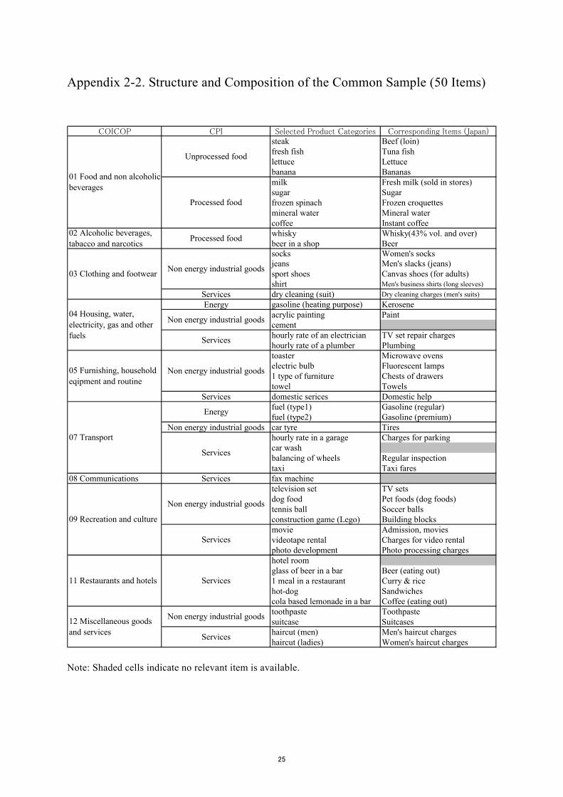
Appendix 2-2. Structure and Composition of the Common Sample (50 Items)

COICOP CPI Selected Product Categories Corresponding Items (Japan)steak Beef (loin)fresh fish Tuna fishlettuce Lettucebanana Bananasmilk Fresh milk (sold in stores)sugar Sugarfrozen spinach Frozen croquettesmineral water Mineral watercoffee Instant coffeewhisky Whisky(43% vol. and over)beer in a shop Beersocks Women's socksjeans Men's slacks (jeans)sport shoes Canvas shoes (for adults)shirt Men's business shirts (long sleeves)

Services dry cleaning (suit) Dry cleaning charges (men's suits)Energy gasoline (heating purpose) Kerosene

acrylic painting Paintcementhourly rate of an electrician TV set repair chargeshourly rate of a plumber Plumbingtoaster Microwave ovenselectric bulb Fluorescent lamps1 type of furniture Chests of drawerstowel Towels

Services domestic serices Domestic helpfuel (type1) Gasoline (regular)fuel (type2) Gasoline (premium)

Non energy industrial goods car tyre Tireshourly rate in a garage Charges for parkingcar washbalancing of wheels Regular inspectiontaxi Taxi fares

08 Communications Services fax machinetelevision set TV setsdog food Pet foods (dog foods)tennis ball Soccer ballsconstruction game (Lego) Building blocksmovie Admission, moviesvideotape rental Charges for video rentalphoto development Photo processing chargeshotel roomglass of beer in a bar Beer (eating out)1 meal in a restaurant Curry & ricehot-dog Sandwichescola based lemonade in a bar Coffee (eating out)toothpaste Toothpastesuitcase Suitcaseshaircut (men) Men's haircut chargeshaircut (ladies) Women's haircut charges

01 Food and non alcoholicbeverages

02 Alcoholic beverages,tabacco and narcotics

03 Clothing and footwear

04 Housing, water,electricity, gas and otherfuels

Energy

Services

05 Furnishing, householdeqipment and routine

07 Transport

09 Recreation and culture

11 Restaurants and hotels

Non energy industrial goods

Services

Non energy industrial goods

Processed food

Non energy industrial goods

Services

Services

Non energy industrial goods

Services

12 Miscellaneous goodsand services

Unprocessed food

Processed food

Non energy industrial goods

Note: Shaded cells indicate no relevant item is available.

25 25

Appendix 3. Criterion for judging whether the distribution has a dip

In this paper, we consider that a distribution of the size of price changes has a dip

(extremely low frequency) nearest to zero percent if the criterion below is fulfilled.

Criterion

If an item has an actual distribution of the size of price changes whose frequency nearest to

zero is smaller than that of a standard normal distribution, we label it as an item which has

a dip nearest to zero percent.

1. Definition of the frequency nearest to zero for the actual distribution (The figure below)

For the actual distribution, Frequency between -2% +2% <Area A in the figure below>Frequency between -10% +10% <Area B in the figure below>

～

～

2. Definition of the frequency nearest to zero for the standard normal distribution

For the standard normal distribution,

(-2%+ ) (+2%+ )Frequency between

(-10%+ ) (+10%+ )Frequency between

μ μσ

μ μσ

～

～

,where μ and σ denote the average size and standard deviation of price changes,

respectively.

-20% -10% 0% 10% 20%2%-2%

A

BB

Size of price changes

26 26

Appendix 4. Calculation Method of Share of Labor Costs

In this appendix, we explain a calculation method of share of labor costs using “2000

Input-Output Table,” conducted by Ministry of Internal Affairs and Communications.

Items for Input-Output Table and CPI

We match sectors within 2000 Input-Output Table to our data set (CPI items, CY2000 base)

according to the specification of CPI. We exclude the automobile insurance premium and

various types of fees because the definition of domestic production in Input-Output Table

doesn’t correspond to that of weights in CPI. In addition, we consider a share of labor costs

is 100% for items whose surveyed prices are identical to labor costs, i.e. cost per

man-month, (service charges for plastering, gardening, carpentering, domestic help etc.).

Labor Cost

Labor cost is defined as a sum of “Wages and salaries”, “Contribution of employers to

social insurance”, “Other payments and allowances”, “Operating surplus” from 2000

Input-Output Table. The rationale for including operating surplus is that mixed income

incorporated in operating surplus is reasonably considered as labor cost for sole

proprietors.

An example for an industry mainly consisting of sole proprietors, whose share of labor

costs is high:

Men’s haircut charges

Share of Labor Costs (excluding operating surplus): 30%

Share of Labor Costs (including operating surplus): 69%

In this case, since the haircut industry holds many sole proprietors, labor cost would be

undervalued if mixed income (operating surplus), which is a proprietors’ own income, is

not included. As similar cases are often seen particularly in the service category, we

decided to treat operating surplus as a part of labor cost.

Note that this treatment over-evaluates the labor costs for such industries that consist

of mostly business corporation.

27 27

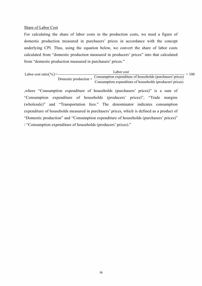
Share of Labor Cost

For calculating the share of labor costs in the production costs, we need a figure of

domestic production measured in purchasers’ prices in accordance with the concept

underlying CPI. Thus, using the equation below, we convert the share of labor costs

calculated from “domestic production measured in producers’ prices” into that calculated

from “domestic production measured in purchasers’ prices.”

( ) Labor costLabor cost ratio % = × 100Consumption expenditure of households (purchasers' prices)Domestic production × Consumption expenditure of households (producers' prices)

,where “Consumption expenditure of households (purchasers’ prices)” is a sum of

“Consumption expenditure of households (producers’ prices)”, “Trade margins

(wholesale)” and “Transportation fees.” The denominator indicates consumption

expenditure of households measured in purchasers’ prices, which is defined as a product of

“Domestic production” and “Consumption expenditure of households (purchasers’ prices)”

/ “Consumption expenditure of households (producers’ prices).”

28 28

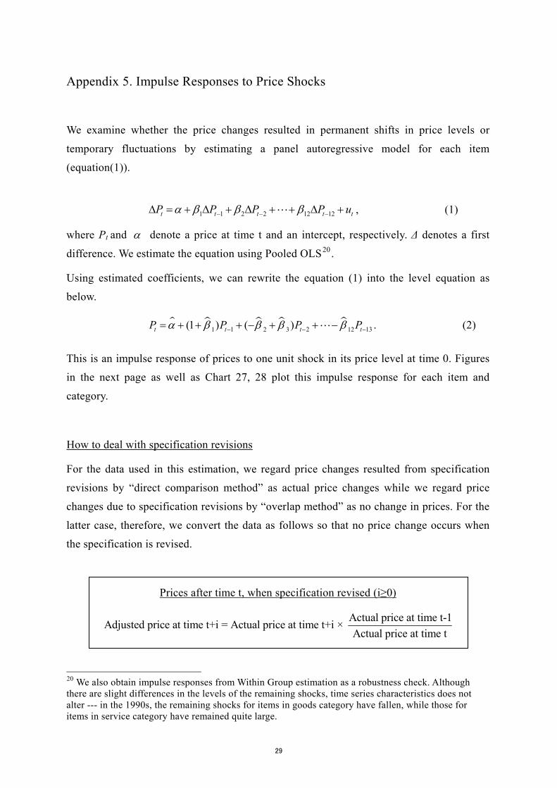
Appendix 5. Impulse Responses to Price Shocks

We examine whether the price changes resulted in permanent shifts in price levels or

temporary fluctuations by estimating a panel autoregressive model for each item

(equation(1)).

1 1 2 2 12 12t t t tP P P P tuα β β β− − −Δ = , (1) + Δ + Δ + + Δ +

where Pt and α denote a price at time t and an intercept, respectively. Δ denotes a first

difference. We estimate the equation using Pooled OLS20.

Using estimated coefficients, we can rewrite the equation (1) into the level equation as

below.

1 21 2 3 1(1 ) ( )t t tP P Pα β β β β− −= + + + − + + − 132 tP− . (2)

This is an impulse response of prices to one unit shock in its price level at time 0. Figures

in the next page as well as Chart 27, 28 plot this impulse response for each item and

category.

How to deal with specification revisions

For the data used in this estimation, we regard price changes resulted from specification

revisions by “direct comparison method” as actual price changes while we regard price

changes due to specification revisions by “overlap method” as no change in prices. For the

latter case, therefore, we convert the data as follows so that no price change occurs when

the specification is revised.

Prices after time t, when specification revised (i≥0)

Actual price at time t-1Adjusted price at time t+i = Actual price at time t+i × Actual price at time t

20 We also obtain impulse responses from Within Group estimation as a robustness check. Although there are slight differences in the levels of the remaining shocks, time series characteristics does not alter --- in the 1990s, the remaining shocks for items in goods category have fallen, while those for items in service category have remained quite large.

29 29

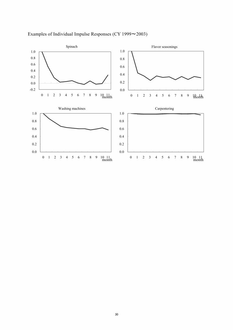
Examples of Individual Impulse Responses (CY 1999～2003)

Spinach

-0.2

0.0

0.2

0.4

0.6

0.8

1.0

0 1 2 3 4 5 6 7 8 9 1

Flavor seasonings

0.0

0.2

0.4

0.6

0.8

1.0

0 1 2 3 4 5 6 7 8 9 10 110 11

Washing machines

0.0

0.2

0.4

0.6

0.8

1.0

0 1 2 3 4 5 6 7 8 9 10 11

Carpentering

0.0

0.2

0.4

0.6

0.8

1.0

0 1 2 3 4 5 6 7 8 9

month month

10 11month month

30 30

Reference

(In English)

・ Álvarez, Luis J., Pablo Burriel, and Ignacio Hernando [2005], “Do decreasing hazard functions for price changes make any sense?,” European Central Bank

Working Paper Series 461, March 2005.

・ Aucremanne, Luc, and Emmanuel Dhyne [2005], “Time-dependent versus state-dependent pricing: A panel data approach to the determinants of Belgian

consumer price changes,” European Central Bank Working Paper Series 462,

March 2005.

・ Bank of Japan, Research and Statistics Department [2000], “Price-setting behavior of Japanese companies –The results of “Survey of price-setting behavior of

Japanese companies” and its analysis–,” Bank of Japan Research Papers.

・ Baudry, Laurent, Hervé Le Bihan, Patrick Sevestre and Sylvie Tarrieu [2004], “Price rigidity: Evidence from the French CPI micro-data,” European Central Bank

Working Paper Series 384, August 2004.

・ Baumgartner, Josef, Ernst Glatzer, Fabio Rumler, and Alfred Stiglbauer [2005], “How frequently do consumer prices change in Austria? Evidence from micro CPI

data,” European Central Bank Working Paper Series 523, September 2005.

・ Bils, Mark, and Peter J. Klenow [2004], “Some Evidence on the Importance of Sticky Prices,” Journal of Political Economy, 112-5, 2004.

・ Blinder, S. Alan, Elie R. D. Canetti, David E. Lebow, and Jeremy B. Rudd [1998], Asking about prices: A new approach to understanding price stickiness, Russel Sage

Foundation, 1998.

・ Calvo, Guillermo A. [1983], “Staggered prices in a utility-maximizing framework,” Journal of Monetary Economics, 12:383-398, 1983.

・ Caplin Andrew S., and Daniel F.Spulber [1987], “Menu costs and the Neutrality of Money,” Quarterly Journal of Economics, 102:703-725.

・ Dhyne, Emmanuel, Luis J. Álvarez, Hervé Le Bihan, Giovanni Veronese, Daniel Dias, Johannes Hoffman, Nicole Jonker, Patrick Lünnemann, Fabio Rumler, and

Jouko Vilmunen [2006], “Price changes in the Euro area and the United States:

Some facts from individual consumer price data,” Journal of Economic Perspectives

31 31

vol.20, Number 2, pp.171-192.

・ Dotsey, M., Robert G. King, and Alexander L. Wolman [1999], “State-Dependent Pricing and the General Equilibrium Dynamics of Money and Output,” Quarterly

Journal of Economics, 114:655-690.

・ Enomoto, Hidetaka [2007], “Multi-sector menu cost model, decreasing hazard, and Phillips curve,” Bank of Japan Working Paper Series 07-E-3.

・ Golosov, Mikhail, and Robert E. Lucas, Jr. [2007], “Menu costs and Phillips curves,” Journal of Political Economy vol.115, Number 2.

・ Ikeda, Daisuke and Shinichi Nishioka [2007], “Price Setting Behavior and Hazard functions: Evidence from Japanese CPI micro data,” Bank of Japan Working Paper

Series 07-E-19.

・ Klenow, Peter. J, and Oleksiy Kryvtsov [2005], “State-dependent or time-dependent pricing: Does it matter for recent U.S. inflation?,” NBER Working Paper Series

11043.

・ Kuroda, Sachiko and Isamu Yamamoto [2005], “Wage Fluctuations in Japan after the Bursting of the Bubble Economy: Downward Nominal Wage Rigidity, Payroll,

and the Unemployment Rate,” Bank of Japan Monetary and Economic Studies

Vol.23, No.2.

・ Nakamura, Emi, and Jón Steinsson [2007], “Five facts about prices: A reevaluation of menu cost models,” mimeo.

・ Taylor, John B. [1979], “Staggered wage setting in a macro model,” American Economic Review, 69:108-113.

・ Veronese, Giovanni, Silvia Fabiani, Angela Gattulli, and Roberto Sabbatini [2005], “Consumer price behaviour in Italy: Evidence from micro CPI data,” European

Central Bank Working Paper Series 449.

(In Japanese)

・ Sakura, Kenichi, Hitoshi Sasaki, Masahiro Higo [2005], “Economic development in

Japan since the 1990s – fact finding-,” Bank of Japan Working Paper Series 05-J-10.

32 32

(1) Items by Category (CY2000 base)

(2) Items Excluded from the analysis (CY2000 base)

Note: For the reasons for exclusion, see p.4 of this paper.

Chart 1. Items by Category

reasons forexclusion

number ofitems items

a) 19

Fire insurance premium, Medical treatment, Railway fares(ordinary fares, for"Shinkansen"), Airplanefares, Automobiles less than 660cc, Automobiles A/B, Automobiles less than 2000cc(imported),Automobiles more than 2000cc, Automobiles more than 2000cc(imported), Telephone charges, Mobiletelephone charges, Package tours to overseas, Imputed rent houses, Personal computers(desktop/notes)Bonito, Oysters, Green soybeans, Apples A/B, Mandarin oranges, Iyo-mandarins, Pears, Grapes A/B,Persimmons, Peaches, Watermelons, Melons, Strawberries, Cherries, Fan heaters, "Kotatsu", Japaneseelectric heaters, Electric carpets, Blankets, Men's suits, Men's jackets, Men's slacks, Men's coats,Boys'school uniforms, Women's suits, One-piece dresses, Skirts, Women's slacks, Women's coatsWomen's jackets, Girls’school uniforms, Girls'skirts, Men's business shirts, Sport shirts, Men's sweaters,Blouses, Women's T-shirts, Women's sweaters, Children's T-shirts, Children's sweaters, Men's undershirts,Men's underpants, Men's pajamas, Mufflers, Men's socks, Children's tights, Desks, School knapsacks,Admission(soccer, progessional baseball games)

c) 7 House rent(private, public, public corporation), Hotel charges

d) 12Personal computers printer, Word processors, Face cream-A, Milky lotion-A, Foundation-A, Lipsticks-A,Monthly magazines(boys', hobbies & cultures, living informations, personal computers, women's), Internetconnection fee

b) 67

CPI ourdataset

598 493 ―

456 372 ―

Fresh food 61 45 Tuna fish, Lettuce, Bananas

Food, excluding fresh food 11 11 Beef, Pork, Hen eggs, Cut flowersOther agricultural &aquatic products 6 6 Rice, Designated standard rice, Red beans

Food products 126 126 Butter, Cakes, Beer

Textiles 73 29 Quilts, Women's dresses, Neckties

Petroleum products 4 4 Liquefied propane, Kerosene, Gasoline

Other industrial products 159 140 Refrigerators, Wardrobes, Facial tissue, Medicines forcold, Rings, Cigarettes

3 3 Electricity, Gas, Water charges

13 8 School textbooks, Newspapers, Books, Weeklymagazines

142 121 ―House rent, public & publiccorporation 2 0 ―

Services related todomestic duties 12 11 Sewerage charges, Automotive insurance premium,

Charges for certificates of registered stampsServices related to medicalcare & welfare 3 2 Nursery school fees, Day service fees of nursing care

for the agedServices related totransportation &communication

22 18 Railway fares(ordinary fares, excluding"Shinkansen"),Bus fares, Postcards

Services related toeducation 3 3 College & university fees(national), Kindergarten

fees(public)Services related to reading& recreation 6 6 Fees for TV viewers, Admission fees to the art

museumEating out 21 21 Japanese noodles, Hamburgers, School lunchPrivate house rent 4 0 ―

Imputed rent 4 0 ―

Services related todomestic duties 28 28 Carpentering, Automotive maintenance charges, Men's

haircut charges, Charges for transfer commission

Services related to medicalcare & welfare 4 4 Delivery fees in hospital, Charges for massage

Services related toeducation 8 8 PTA menbership fees, College & university

fees(private), Tutorial feesServices related to reading& recreation 25 20 Lesson fees, Admission(movies), Admission fees to the

recreation ground, Veterinary surgeon fees

General services

Industrial products

Agricultural &aquatic products

Electricity, Gas & Water charges

Publications

Services

Public services

Goods

Total

Examplesnumber of items

33

CoverageCPI our dataset (%)

CY1990 Base 561 476 84.8

CY1995 Base 580 493 85.0

CY2000 Base 598 493 82.4

(%)

1990 1995 2000 CPI our dataset

Total 73.2 70.5 68.0 100.0 100.0Total, excluding imputed rent 81.3 81.4 78.6 86.4 100.0Total, excluding fresh food 73.0 70.2 67.5 95.5 94.9Total, excluding imputed rent & fresh food 81.6 81.7 78.7 81.9 94.9

Goods 84.7 86.1 84.7 50.8 63.3

Agricultural & aquatic products 87.1 87.1 86.6 7.8 9.9Fresh agricultural & aquatic products 84.5 84.8 84.5 6.7 8.3

Fresh food 76.9 77.5 76.8 4.5 5.1Food,excluding fresh food 100.0 100.0 100.0 2.2 3.3

Other agricultural & aquatic products 100.0 100.0 100.0 1.0 1.5

Industrial products 81.8 83.5 82.1 36.5 44.1Food products 100.0 100.0 100.0 13.7 20.2Textiles 39.1 39.2 40.7 5.6 3.4Petroleum products 100.0 100.0 100.0 3.0 4.4Other industrial products 85.1 85.0 77.3 14.1 16.1

Electricity, gas & water charges 100.0 100.0 100.0 4.8 7.1Publications 100.0 100.0 90.7 1.7 2.3

Services 58.8 53.9 50.6 49.2 36.7Services, excluding imputed rent 75.7 74.6 70.0 35.6 36.7

Public services 58.7 60.5 56.4 12.9 10.7House rent, public & public corporation 0.0 0.0 0.0 0.5 0.0Services related to domestic duties 76.0 82.0 84.6 3.0 3.7Services related to medical care & welfare ― ― 19.8 2.0 0.6Services related to transportation & communication 62.2 61.3 45.7 5.6 3.8Services related to education 100.0 100.0 100.0 0.6 0.9Services related to reading & recreation 100.0 100.0 100.0 1.2 1.7

General services 58.8 52.0 48.6 36.3 25.9General services, excluding imputed rent 83.6 81.0 77.7 22.7 25.9

Eating out 100.0 100.0 100.0 6.2 9.1Private house rent 0.0 0.0 0.0 3.0 0.0Imputed rent 0.0 0.0 0.0 13.6 0.0Other services 88.9 90.1 84.7 13.5 16.8

Services related to domestic duties 100.0 100.0 100.0 4.8 7.1Services related to medical care & welfare 100.0 100.0 100.0 0.3 0.5Services related to education 100.0 100.0 100.0 3.3 4.8Services related to reading & recreation 71.9 72.6 59.4 5.1 4.4

Chart 2. Data Coverage

Coverage Weight

Number of Items

34

(1) Number of Samples Collected by City

Number ofCities GroupA GroupB GroupC GroupD

Cities with prefectural government other than16 major large cities 33 4 3 2 1

Cities with population 150,000 or more(excl. cities with prefectural government ) 22 4 3 1 1

Note: 16 major large cities include Tokyo, Osaka, Yokohama, Kyoto, Kobe, Sapporo, Sendai, Chiba, Kawasaki, Hiroshima, Fukuoka, Kitakyushu, Kanazawa, Takamatsu, Naha.

(2) Average Number of Samples by Category

(a) Total, Goods, and Services

(b) Goods by Category

(c) Services by Category

Chart 3. Number of Samples Prices by City and Category

2.7 2.92.4

1.1

3.0

0.0

0.5

1.0

1.5

2.0

2.5

3.0

3.5

Total Goods Services Public services General services

（％）

4.0 4.0 3.9

3.32.9

4.0

2.6 2.4 2.4

1.0 1.0

0.00.51.01.52.02.53.03.54.04.5

Fresh food Food,excl.fresh food

Otheragricultural

& aquaticproducts

Foodproducts

Textiles Petroleumproducts

Durablegoods

Semi-durablegoods

Non-durablegoods

Electricity,gas & water

charges

Publications

（％）

1.0 1.0 1.1 1.0 1.1

3.12.7

1.9

3.6

2.8

0.00.51.01.52.02.53.03.54.04.5

Domesticduties

Medical care & welfare

Transportation &

communication

Education Reading &recreation

Eating out Domesticduties

Medical care & welfare

Education Reading &recreation

（％）

Public Services General Services

35

(1) Total, Goods, and Services

(2) Goods by Category

(3) Services by Category

Chart 4. Average Frequency of Price Changes (CY 1999 to CY 2003)

21.4

4.5 3.9 4.7

31.1

0

5

10

15

20

25

30

35

Total Goods Services Public services General services

(%/month)

53.5

34.429.9

14.6

36.9

27.3

14.2 16.720.5

6.3

0

10

20

30

40

50

60

Fresh food Food,excl.fresh food

Otheragricultural & aquaticproducts

Foodproducts

Textiles Petroleumproducts

Durablegoods

Semi-durablegoods

Non-durablegoods

Electricity,gas & water

charges

Publications

(%/month)

91.1

8.81.8 0.3

5.51.4

5.0 2.65.8 6.2 6.0

0

10

20

30

40

50

60

Domestic duties

Medical care & welfare

Transportation &

communication

Education Reading &recreation

Eating out Domestic duties

Medical care & welfare

Education Reading &recreation

(%/month)

Public Services General Services

36

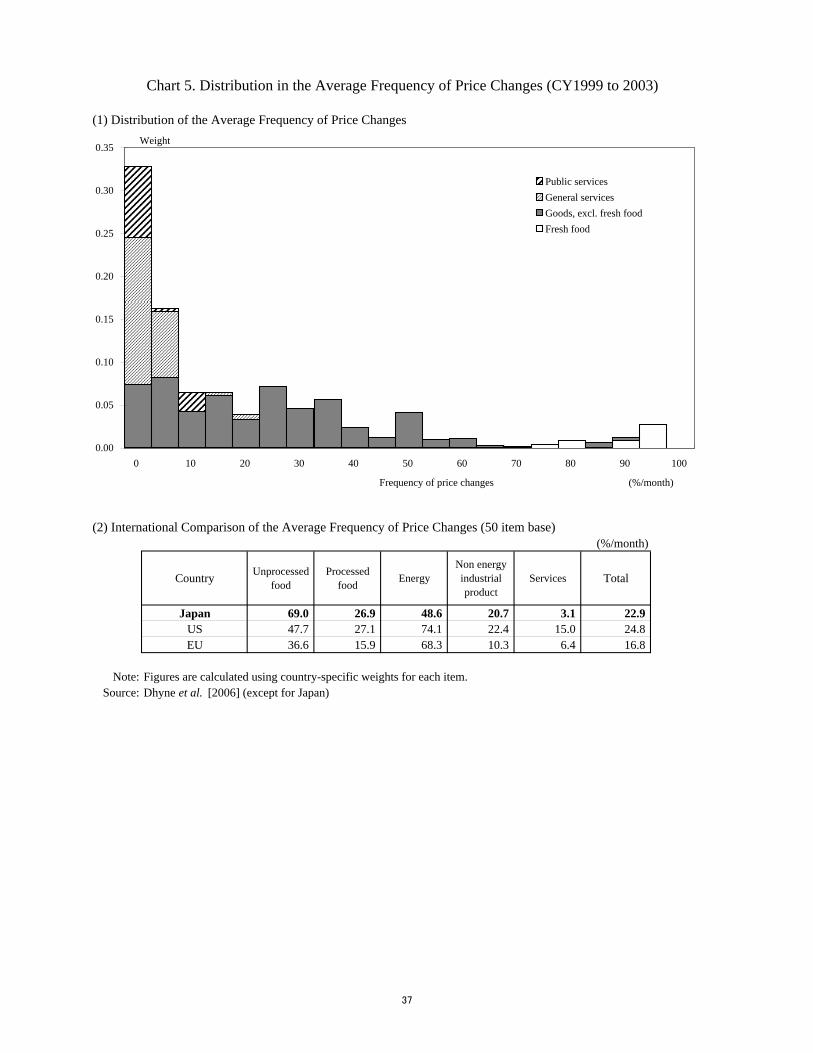
(1) Distribution of the Average Frequency of Price Changes

(2) International Comparison of the Average Frequency of Price Changes (50 item base)(%/month)

Country Unprocessed food

Processed food Energy

Non energy industrial product

Services Total

Japan 69.0 26.9 48.6 20.7 3.1 22.9US 47.7 27.1 74.1 22.4 15.0 24.8EU 36.6 15.9 68.3 10.3 6.4 16.8

Note: Figures are calculated using country-specific weights for each item.Source: Dhyne et al. [2006] (except for Japan)

Chart 5. Distribution in the Average Frequency of Price Changes (CY1999 to 2003)

0.00

0.05

0.10

0.15

0.20

0.25

0.30

0.35

0 10 20 30 40 50 60 70 80 90 100

Frequency of price changes (%/month)

Weight

Public servicesGeneral servicesGoods, excl. fresh foodFresh food

37

(1) Total, Goods, and Services

(2) Goods, by Category

(3) Services, by Category

Chart 6. Average Frequency of Price Increases and Decreases (CY1999 to 2003)

0

2

4

6

8

10

12

14

16

18

Total Goods Services Public services General services

Frequency of price increasesFrequency of price decreases

(%)

0

5

10

15

20

25

30

35

40

45

50

Fresh food Food,excl. freshfood

Other agricultural& aquaticproducts

Food products Textiles Petroleumproducts

Other industrialproducts

Electricity, gas &water charges

Publications

Frequency of price increasesFrequency of price decreases

(%)

0

1

2

3

4

5

6

Domestic duties Medical care &welfare

Transportation & communication

Education Eating out Domestic duties Medical care &welfare

Education Reading &recreation

Frequency of price increasesFrequency of price decreases

(%)

Public Services General Services

38

(1) Total

(2) Goods

(3) Services

Chart 7. Frequency of Price Changes by Year(CY1989-2003)

15

16

17

18

19

20

21

22

23

24

25

1989 1990 1991 1992 1993 1994 1995 1996 1997 1998 1999 2000 2001 2002 2003 CY-1.5

-1.0

-0.5

0.0

0.5

1.0

1.5

2.0

2.5

3.0

3.5

4.0

Frequency of Price ChangesInflation Rate (CPI, Total) <Right Scale>

(%/month)

20

22

24

26

28

30

32

34

36

1989 1990 1991 1992 1993 1994 1995 1996 1997 1998 1999 2000 2001 2002 2003 CY-2.0

-1.0

0.0

1.0

2.0

3.0

4.0

Frequency of Price ChangesInflation Rate (CPI, Goods) <Right Scale>

(%/month)

2

3

4

5

6

7

8

9

10

11

12

1989 1990 1991 1992 1993 1994 1995 1996 1997 1998 1999 2000 2001 2002 2003 CY-0.5

0.0

0.5

1.0

1.5

2.0

2.5

3.0

3.5

Frequency of Price ChangesInflation Rate (CPI, Services) <Right Scale>

(%/month)

39

(1) Agricultural & aquatic products, Fresh foods, Other fresh foods, Other agricultural & aquatic products

(2) Food products, Textiles, Petroleum products, & Other industrial products (durable goods, semi-durable goods, & non-durable goods)

(3) Petroleum products, Electricity,city gas & water charges, & Publications

Chart 8. Frequency of Price Changes by Year (CY1989 to 2003): Goods

0

10

20

30

40

50

60

70

80

90

100

1989 1990 1991 1992 1993 1994 1995 1996 1997 1998 1999 2000 2001 2002 2003

CY

Freq

uenc

y of

Pric

e C

hang

es

Agricultural & aquatic productsFresh foodsOther fresh foodsOther agricultural & aquatic products

(%/month)

0

5

10

15

20

25

30

35

40

1989 1990 1991 1992 1993 1994 1995 1996 1997 1998 1999 2000 2001 2002 2003

CY

Freq

uenc

y of

Pric

e C

hang

es

Food productsTextilesOther industrial products(Durable)Other industrial products(Semi-durable)Other industrial products(Non-durable)

(%/month)

0

5

10

15

20

25

30

35

40

45

50

1989 1990 1991 1992 1993 1994 1995 1996 1997 1998 1999 2000 2001 2002 2003

CY

Freq

uenc

y of

Pric

e C

hang

es

Petroleum productsElectricity,city gas & water chargesPublications

(%/month)

40

(1) Public and General Services

(2) Breakdown of Public services

(3) Breakdown of General services

Chart 9. Frequency of Price Changes by Year (CY1989 to 2003): Services

0

2

4

6

8

10

12

14

16

18

1989 1990 1991 1992 1993 1994 1995 1996 1997 1998 1999 2000 2001 2002 2003

CY

Freq

uenc

y of

Pric

e C

hang

es

Domestic dutiesMedical care & welfareTransportation & communicationEducationReading & recreation

(%/month)

0

2

4

6

8

10

12

14

16

18

20

1989 1990 1991 1992 1993 1994 1995 1996 1997 1998 1999 2000 2001 2002 2003

CY

Freq

uenc

y of

Pric

e C

hang

es

Eating outDomestic dutiesMedical care & welfareEducationReading & recreation

(%/month)

0

2

4

6

8

10

12

14

1989 1990 1991 1992 1993 1994 1995 1996 1997 1998 1999 2000 2001 2002 2003

CY

Freq

uenc

y of

Pric

e C

hang

es

Public services

General services

(%/month)

41

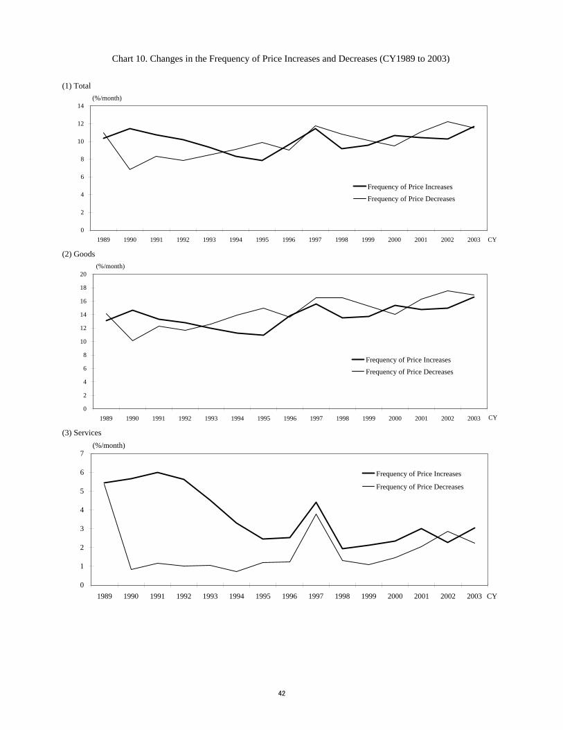
(1) Total

(2) Goods

(3) Services

Chart 10. Changes in the Frequency of Price Increases and Decreases (CY1989 to 2003)

0

2

4

6

8

10

12

14

1989 1990 1991 1992 1993 1994 1995 1996 1997 1998 1999 2000 2001 2002 2003 CY

Frequency of Price IncreasesFrequency of Price Decreases

(%/month)

0

2

4

6

8

10

12

14

16

18

20

1989 1990 1991 1992 1993 1994 1995 1996 1997 1998 1999 2000 2001 2002 2003 CY

Frequency of Price IncreasesFrequency of Price Decreases

(%/month)

0

1

2

3

4

5

6

7

1989 1990 1991 1992 1993 1994 1995 1996 1997 1998 1999 2000 2001 2002 2003 CY

Frequency of Price Increases

Frequency of Price Decreases

(%/month)

42

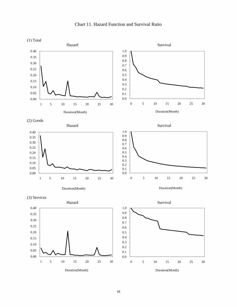
(1) Total

(2) Goods

(3) Services

Chart 11. Hazard Function and Survival Ratio

Hazard Survival

Hazard Survival

Hazard Survival

0.000.050.100.150.200.250.300.350.40

1 5 10 15 20 25 30

Duration(Month)

0.00

0.05

0.10

0.15

0.20

0.25

0.30

0.35

0.40

1 5 10 15 20 25 30

Duration(Month)

0.00.10.20.30.40.50.60.70.80.91.0

0 5 10 15 20 25 30

Duration(Month)

0.00.10.20.30.40.50.60.70.80.91.0

0 5 10 15 20 25 30

Duration(Month)

0.00

0.05

0.10

0.15

0.20

0.25

0.30

0.35

0.40

1 5 10 15 20 25 30

Duration(Month)

0.00.10.20.30.40.50.60.70.80.91.0

0 5 10 15 20 25 30

Duration(Month)

43

(1) Flexible

(2) Downward sloping

(3) Taylor

Chart 12. Hazard Function by Type

Goods

Services

Fresh food, Hen Eggs, Cut Flowers

None

Category (Item)

Category (Item)

Goods Items other than Fresh food and Electricity and gas charges

Services General Services (Eating out, Domestic duties, and Reading and recreation)

Category (Item)

Goods Electricity and gas charges

Services

Public Services, General Services (Medical care & welfare, Education, a

part of Reading and recreation <Lesson fees>)

Duration(Month)

Hazard

Duration(Month)

Hazard

12 24Duration(Month)

Hazard

44

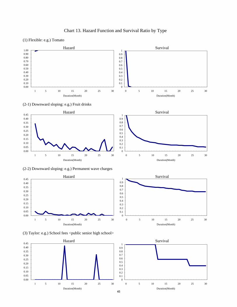
(1) Flexible: e.g.) Tomato

(2-1) Downward sloping: e.g.) Fruit drinks

(2-2) Downward sloping: e.g.) Permanent wave charges

(3) Taylor: e.g.) School fees <public senior high school>

Hazard

Survival

Survival

Survival

Survival

Chart 13. Hazard Function and Survival Ratio by Type

Hazard

Hazard

Hazard

0.000.100.200.300.400.500.600.700.800.901.00

1 5 10 15 20 25 30

Duration(Month)

0.000.050.100.150.200.250.300.350.400.45

1 5 10 15 20 25 30

Duration(Month)

0.000.050.100.150.200.250.300.350.400.45

1 5 10 15 20 25 30

Duration(Month)

0.000.050.100.150.200.250.300.350.400.45

1 5 10 15 20 25 30

Duration(Month)

00.10.20.30.40.50.60.70.80.9

1

0 5 10 15 20 25 30

Duration(Month)

00.10.20.30.40.50.60.70.80.9

1

0 5 10 15 20 25 30

Duration(Month)

00.10.20.30.40.50.60.70.80.9

1

0 5 10 15 20 25 30

Duration(Month)

00.10.20.30.40.50.60.70.80.9

1

0 5 10 15 20 25 30

Duration(Month)

45

(1) Total

(2) Goods

(3) Services

Hazard Survival

Hazard Survival

Chart 14. Changes in the Hazard Function and the Survival RatioCY1989 to 1993→CY1999 to 2003

Hazard Survival

0.00

0.05

0.10

0.15

0.20

0.25

0.30

0.35

0.40

1 5 10 15 20 25 30

Duration(Month)

1989-1993

1999-2003

0.00

0.05

0.10

0.15

0.20

0.25

0.30

0.35

0.40

1 5 10 15 20 25 30

Duration(Month)

1989-1993

1993-2003

0.00

0.05

0.10

0.15

0.20

0.25

0.30

0.35

0.40

1 5 10 15 20 25 30

Duration(Month)

1989-1993

1999-2003

0.0

0.1

0.2

0.3

0.4

0.5

0.6

0.7

0.8

0.9

1.0

0 5 10 15 20 25 30

Duration(Month)

1989-1993

1999-2003

0.0

0.1

0.2

0.3

0.4

0.5

0.6

0.7

0.8

0.9

1.0

0 5 10 15 20 25 30

Duration(Month)

1989-1993

1993-2003

0.0

0.1

0.2

0.3

0.4

0.5

0.6

0.7

0.8

0.9

1.0

0 5 10 15 20 25 30

Duration(Month)

1989-1993

1999-2003

46

(1) By Cagetory

(a) Food Products (b) General Services, domestic duties

(2) By Item

(a) Beer (b) Plumbing

Chart 15. Changes in the Hazard Function

0.00

0.02

0.04

0.06

0.08

0.10

0.12

1 5 10 15 20 25 30

Duration(Month)

1989-1993

1999-2003

0.00

0.05

0.10

0.15

0.20

0.25

0.30

0.35

0.40

0.45

1 5 10 15 20 25 30

Duration(Month)

1989-1993

1999-2003

0.00

0.10

0.20

0.30

0.40

0.50

0.60

1 5 10 15 20 25 30

Duration(Month)

1989-19931999-2003

0.00

0.02

0.04

0.06

0.08

0.10

0.12

0.14

0.16

0.18

0.20

1 5 10 15 20 25 30

Duration(Month)

1989-19931999-2003

47

(1) Total, Goods, and Services

(2) Goods by Category

(3) Services by Category

Chart 16. Average Size of Price Changes (CY1999 to 2003)

0

2

4

6

8

10

12

14

16

18

Total Goods Services Public services General services

Average size of price increasesAverage size of price decreases

(%)

0

2

4

6

8

10

12

14

16

18

Fresh food Food,excl. freshfood

Other agricultural& aquaticproducts

Food products Textiles Petroleumproducts

Other industrialproducts

Electricity, gas &water charges

Publications

Average size of price increases

Average size of price decreases

(%)

0

2

4

6

8

10

12

14

16

18

Domestic duties Medical care &welfare

Transportation & communication

Education Eating out Domestic duties Medical care &welfare

Education Reading &recreation

Average size of price increases

Average size of price decreases

(%)

Public Services General Services

48

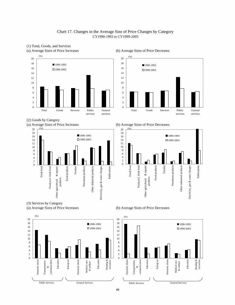
(1) Total, Goods, and Services(a) Average Sizes of Price Increases (b) Average Sizes of Price Decreases

(2) Goods by Category(a) Average Sizes of Price Increases (b) Average Sizes of Price Decreases

(3) Services by Category(a) Average Sizes of Price Increases (b) Average Sizes of Price Decreases

CY1990-1993 to CY1999-2003Chart 17. Changes in the Average Size of Price Changes by Category

0

2

4

6

8

10

12

14

16

18

20

Total Goods Services Publicservices

Generalservices

1990-1993

1999-2003

(%)

02468

101214161820

Dom

estic

dut

ies

Tran

spor

tatio

n

&co

mm

unic

atio

n

Educ

atio

n

Eatin

g ou

t

Dom

estic

dut

ies

Med

ical

car

e

& w

elfa

re

Educ

atio

n

Rea

ding

&re

crea

tion

(%)

1990-19931999-2003

Public Services General Services

02468

101214161820

Dom

estic

dut

ies

Tran

spor

tatio

n

&co

mm

unic

atio

n

Educ

atio

n

Eatin

g ou

t

Dom

estic

dut

ies

Med

ical

car

e

& w

elfa

re

Educ

atio

n

Rea

ding

&re

crea

tion

(%)

1990-1993

1999-2003

Public Services General Services

02468

101214161820

Fres

h fo

od

Food

,exc

l. fr

esh

food

Oth

er a

gric

ultu

ral

& a

quat

icpr

oduc

ts

Food

pro

duct

s

Text

iles

Petro

leum

pro

duct

s

Oth

er in

dust

rial p

rodu

cts

Elec

trici

ty, g

as &

wat

er c

harg

es

Publ

icat

ions

1990-19931999-2003

(%)

02468

101214161820

Fres

h fo

od

Food

,exc

l. fr

esh

food

Oth

er a

gric

ultu

ral

& a

quat

icpr

oduc

ts

Food

pro

duct

s

Text

iles

Petro

leum

pro

duct

s

Oth

er in

dust

rial p

rodu

cts

Elec

trici

ty, g

as &

wat

er c

harg

es

Publ

icat

ions

1990-1993

1999-2003

(%)

0

2

4

6

8

10

12

14

16

18

20

Total Goods Services Publicservices

Generalservices

1990-1993

1999-2003

(%)

49

Changes in the inflation rate is broken down as below. Figures are in annual.

Inflation rate (π) = (Frequency of price increases (Fi) * Average size of a price increase (Si)) + (Frequency of price decreases (Fd ) * Average size of a price decrease (Sd ))

Thus, changes in the inflation rate is defined as

where subscript 1 and 2 denote CY1990-1993 and CY1999-2003, respectively.

As shown below, equation 2 can be solved in two ways depending on the base year.

Figures in the chart above is the averaged contributions of A and B.

Chart 18-1. Breakdown of the Changes in Inflation Rate (1)CY1990-1993 to CY1999-2003

{ }

{ }

1 1 1 1 1 1 1 1

1 1 1 1

2 2 2 2 ,2 ,2 ,2 2

2 2 2 2

( )( ) ( )( ) ( )

( ) ( )( ) ( )( )

u u u u d d d d u u d d

u u d d u u d d u u d d

u u d d u u u u d d d d

u u d d u u d d u u d

F F S S F F S S F S F SF S F S S F S F F S F S

or

F S F S F F S S F F S S

F S F S S F S F F S F S

π

π

∆ = + ∆ + ∆ − + ∆ + ∆ − −

= ∆ − ∆ + ∆ − ∆ + ∆ ∆ − ∆ ∆

∆ = − − − ∆ − ∆ − − ∆ − ∆

= ∆ − ∆ + ∆ − ∆ − ∆ ∆ + ∆ ∆ d

-7

-6

-5

-4

-3

-2

-1

0

1

2

3

Total Goods Services Public Services General Services

Size of Price DecreasesSize of Price IncreasesFrequency of Price DecreasesFrequency of Price Increases

(%)

i i d dF S F Sπ = −

2 2 2 2 1 1 1 1( ) ( ),u u d d u u d dF S F S F S F Sπ∆ = − − −

Contribution of the Frequency (A)

A

B

(equation 2)

(equation 1)

Contribution of the Size (A)

Contribution of the Frequency (B)

Contribution of the Size (B)

Residuals

Residuals

50

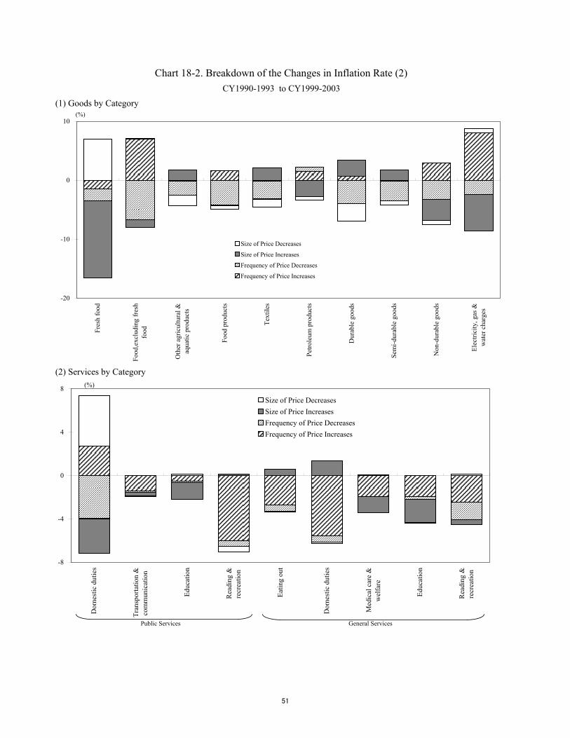
(1) Goods by Category

(2) Services by Category

CY1990-1993 to CY1999-2003

Chart 18-2. Breakdown of the Changes in Inflation Rate (2)

-20

-10

0

10

Fres

h fo

od

Food

,exc

ludi

ng fr

esh

food

Oth

er a

gric

ultu

ral &

aqua

tic p

rodu

cts

Food

pro

duct

s

Text

iles

Petro

leum

pro

duct

s

Dur

able

goo

ds

Sem

i-dur

able

goo

ds

Non

-dur

able

goo

ds

Elec

trici

ty, g

as &

wat

er c

harg

es

Size of Price Decreases

Size of Price Increases

Frequency of Price Decreases

Frequency of Price Increases

(%)

-8

-4

0

4

8

Dom

estic

dut

ies

Tra

nspo

rtatio

n &

com

mun

icat

ion

Edu

catio

n

Rea

ding

&re

crea

tion

Eatin

g ou

t

Dom

estic

dut

ies

Med

ical

car

e &

wel

fare

Edu

catio

n

Rea

ding

&re

crea

tion

Size of Price DecreasesSize of Price IncreasesFrequency of Price DecreasesFrequency of Price Increases

(%)

Public Services General Services

51

Chart 19. Frequency distribution of the Sizes of Price Changes (CY1999-2003)

(1) Lower bounds in the size of price changes exist

(2) No lower bound in the size of price changes

Coffee beverages

0.00

0.02

0.04

0.06

0.08

0.10

0.12

-20% -10% 0% 10% 20%

Freq

uenc

y

Weekly magazines B

0.00

0.05

0.10

0.15

0.20

0.25

0.30

-20% -10% 0% 10% 20%

Freq

uenc

y

Bus fares

0.000.020.040.060.080.100.120.14

-20% -10% 0% 10% 20%

Freq

uenc

y

Game charges, bowling

0.000.020.040.060.080.100.120.140.16

-20% -10% 0% 10% 20%

Freq

uenc

y

Refrigerators

0.00

0.01

0.02

0.03

0.04

0.05

0.06

-20% -10% 0% 10% 20%

Freq

uenc

y

Gas, manufactured & piped

0.00

0.05

0.10

0.15

0.20

-20% -10% 0% 10% 20%

Freq

uenc

y

Schoo fees (private junior high shool)

0.00

0.02

0.04

0.06

0.08

0.10

0.12

-20% -10% 0% 10% 20%

Freq

uenc

y

Rice A

0.00

0.02

0.04

0.06

0.08

0.10

0.12

-20% -10% 0% 10% 20%

Freq

uenc

y

52

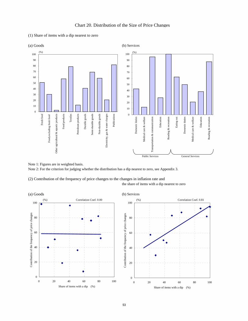
(1) Share of items with a dip nearest to zero

(a) Goods (b) Services

Note 1: Figures are in weighted basis.Note 2: For the criterion for judging whether the distribution has a dip nearest to zero, see Appendix 3.

(2) Contribution of the frequency of price changes to the changes in inflation rate andthe share of items with a dip nearest to zero

(a) Goods (b) Services

Chart 20. Distribution of the Size of Price Changes

0

10

20

30

40

50

60

70

80

90

100

Fres

h fo

od

Food

,exc

ludi

ng fr

esh

food

Oth

er a

gric

ultu

ral &

aqu

atic

pro

duct

s

Food

pro

duct

s

Text

iles

Petro

leum

pro

duct

s

Dur

able

goo

ds

Sem

i-dur

able

goo

ds

Non

-dur

able

goo

ds

Elec

trici

ty, g

as &

wat

er c

harg

es

Publ

icat

ions

(%)

0

10

20

30

40

50

60

70

80

90

100

Dom

estic

dut

ies

Med

ical

car

e &

wel

fare

Tran

spor

tatio

n &

com

mun

icat

ion

Educ

atio

n

Rea

ding

& re

crea

tion

Eatin

g ou

t

Dom

estic

dut

ies

Med

ical

car

e &

wel

fare

Educ

atio

n

Rea

ding

& re

crea

tion

(%)

General ServicesPublic Services

0

20

40

60

80

100

0 20 40 60 80 100

Share of items with a dip (%)

Con

tribu

tion

of th

e fr

eque

ncy

of p

rice

chan

ges

(%) Correlation Coef. 0.00

0

20

40

60

80

100

0 20 40 60 80 100

Share of items with a dip (%)

Con

tribu

tion

of th

e fr

eque

ncy

of p

rice

chan

ges

(%) Correlation Coef. 0.81

53

(1) By Category

(2) By Item (Excluding Fresh Food)

Note1: For the definition of labor cost share, see the Appendix 5. Note2: In Figure(1), labor cost share is weighted average using CPI weight (CY2000 base).Source: Ministry of Internal Affairs and Communication, "2000 Input-Output Table."

Chart 21. Share of Labor Costs and Frequency of Price Changes

0

10

20

30

40

50

60

70

80

90

100

0 10 20 30 40 50 60 70 80 90 100

Share of Labor Costs (CY2000)

Freq

uenc

y of

pric

e ch

ange

s (C

Y19

99-2

003)

Goods

Services

(%)

(%/month)

0

10

20

30

40

50

60

70

80

90

100

0 10 20 30 40 50 60 70 80 90 100

Share of Labor Costs (CY2000)

Freq

uenc

y of

pric

e ch

ange

s (C

Y19

99-2

003)

(%)

(%/month)

54

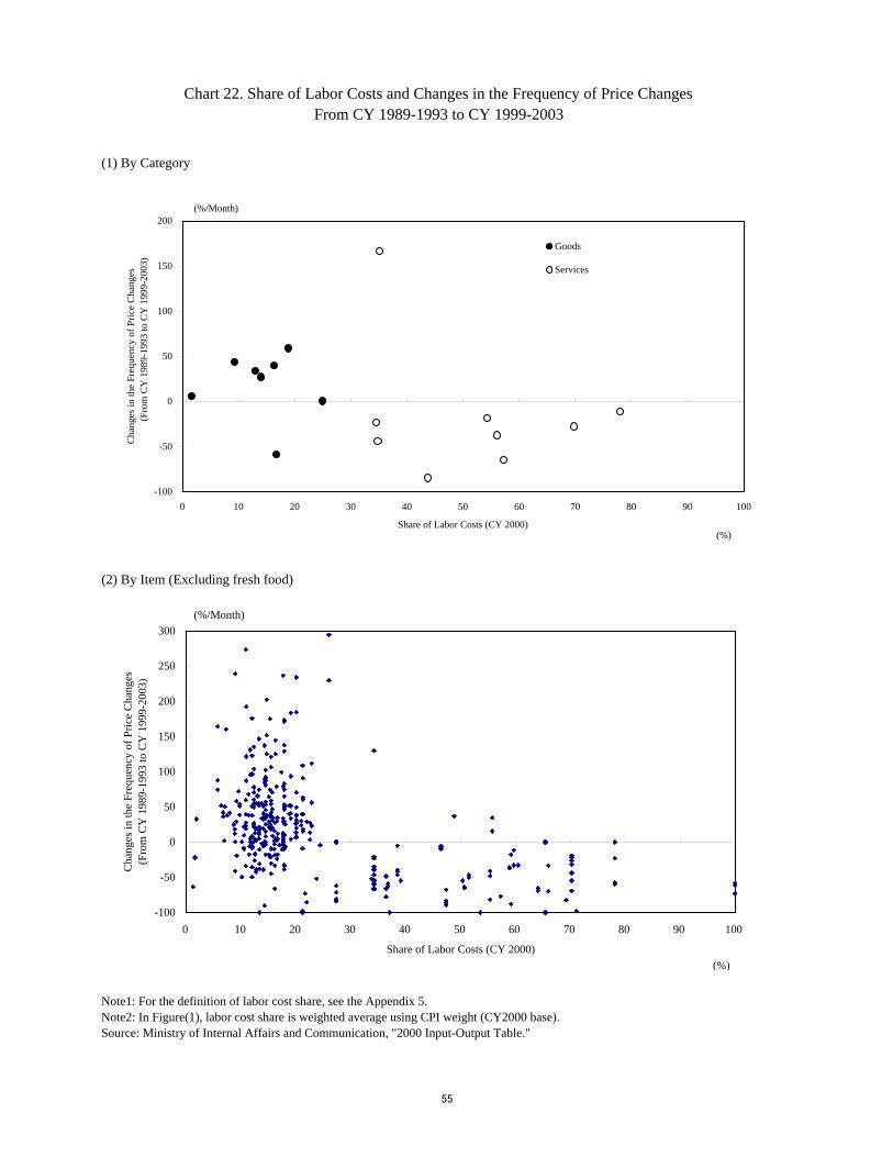
(1) By Category

(2) By Item (Excluding fresh food)

Note1: For the definition of labor cost share, see the Appendix 5. Note2: In Figure(1), labor cost share is weighted average using CPI weight (CY2000 base).Source: Ministry of Internal Affairs and Communication, "2000 Input-Output Table."

Chart 22. Share of Labor Costs and Changes in the Frequency of Price ChangesFrom CY 1989-1993 to CY 1999-2003

-100

-50

0

50

100

150

200

0 10 20 30 40 50 60 70 80 90 100

Share of Labor Costs (CY 2000)

Cha

nges

in th

e Fr

eque

ncy

of P

rice

Cha

nges

(Fro

m C

Y 1

989-

1993

to C

Y 1

999-

2003

)

Goods

Services

(%)

(%/Month)

-100

-50

0

50

100

150

200

250

300

0 10 20 30 40 50 60 70 80 90 100

Share of Labor Costs (CY 2000)

Cha

nges

in th

e Fr

eque

ncy

of P

rice

Cha

nges

(F

rom

CY

198

9-19

93 to

CY

199

9-20

03)

(%/Month)

(%)

55

(1) Change in hourly wages

(2) Share of workers having their wages revised (Full-time workers)

(3) Share of workers having their wages revised (Part-time workers)

Source: Ministry of Health, Labor and Welfare, "Basic Survey on Wage Structure" Ministry of Health, Labor and Welfare, "A look at survey results of reality of wage increase" Japan Bussiness Federation, "Survey results of recent college graduates' wage in March 2004 (2003 Nen 3 Gatsu-Sotsu Shinki-Gakusotsusha Kettei-Shoninkyu Chousa-Kekka ni Tsuite)."

Chart 23. Changes in Wages and Frequency of Wage Revision

-2

0

2

4

6

8

10

1989 1990 1991 1992 1993 1994 1995 1996 1997 1998 1999 2000 2001 2002 2003

(year)

(%)

full-time workerspart-time workers

0

10

20

30

40

50

60

70

80

90

100

1989 1990 1991 1992 1993 1994 1995 1996 1997 1998 1999 2000 2001 2002 2003

(year)

(%)

All workersRecent college graduates

80.1

52.4

34.5

0

10

20

30

40

50

60

70

80

90

1995 2001 2003 (year)

(%)

56

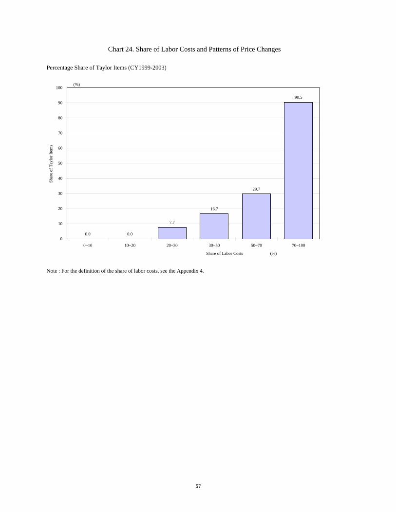
Percentage Share of Taylor Items (CY1999-2003)

Note : For the definition of the share of labor costs, see the Appendix 4.

Chart 24. Share of Labor Costs and Patterns of Price Changes

0.0 0.0

7.7

16.7

29.7

90.5

0

10

20

30

40

50

60

70

80

90

100

0~10 10~20 20~30 30~50 50~70 70~100

Share of Labor Costs (%)

Shar

e of

Tay

lor I

tem

s

(%)

57

(1) Downward nominal rigidity has been continued

(2) Downward nominal rigidity has disappeared.in the 1980s

1999-20031989-1993

1989-1993 1999-2003

Chart 25. Downward Nominal Rigidity in General Service Prices

1989-1993 1999-2003

1989-1993 1999-2003

School fees (Private Senior high school)

0.000.010.020.030.040.050.060.070.080.09

-20% -10% 0% 10% 20%

Freq

uenc

y

Plastering

0.000.010.020.030.040.050.060.070.080.090.10

-20% -10% 0% 10% 20%

Freq

uenc

y

Garage rental charges

0.00

0.02

0.04

0.06

0.08

0.10

0.12

-20% -10% 0% 10% 20%

Freq

uenc

y

Plastering

0.000.010.020.030.040.050.060.070.080.090.10

-20% -10% 0% 10% 20%

Freq

uenc

y

Garage rental charges

0.00

0.01

0.02

0.03

0.04

0.05

0.06

0.07

-20% -10% 0% 10% 20%

Freq

uenc

y

School fees (Private Senior high school)

0.000.020.040.060.080.100.120.140.160.180.20

-20% -10% 0% 10% 20%

Freq

uenc

y

Admissions, movies

0.00

0.05

0.10

0.15

0.20

0.25

0.30

0.35

0.40

-20% -10% 0% 10% 20%

Freq

uenc

y

Admissions, movies

0.000.020.040.060.080.100.120.140.160.18

-20% -10% 0% 10% 20%

Freq

uenc

y

58

(1) Shares of outlets making discount sales (2) Proportions of purchases at supermarkets and discount stores

(3) Proportions of purchases at supermarkets and discount stores and the frequency of price changes (Food products)

Source: Ministry of Internal Affairs and Communication, "Consumer Price Index"; "Annual Report on the Retail Price Survey"; "National Survey of Family Income and Expenditure."

Chart 26. Changes in Competitive Environment Surrounding Retail Businesses

7.7

28.0

41.2

12.0

38.7

46.0

0

10

20

30

40

50

Small size outlets Large supermarkets Mass merchandise outlets

(%)

CY1997

CY2002

60.4

33.3

40.8

50.9

16.619.1

23.2

27.2

42.0

49.3 57.9

21.8

0

10

20

30

40

50

60

70

1984 1994 1999 2004Year

(%)

FoodFurniture & household utensilsClothes & footwear

-100

0

100

200

300

400

500

600

700

800

900

1000

1100

1200

0 5 10 15 20 25 30 35 40 45 50Changes in the proportions

of Supermarkets and Discount stores (CY 1984-1999)

Cha

nges

in th

e fr

eque

ncy

of p

rice

chan

ges (

89-9

3 to

99-

03)

Wine

Whisky B

Whisky C

( % chg.)

( % chg.)

Beer

Whisky A

Spirits

Whisky(imported)

Cola drinks"Sake" C"Sake" B"Sake" A

Wine(imported)

Fruit drinks

Instant soupGranular flavor seasonings

Ice cream

Dried bonito fillets

59

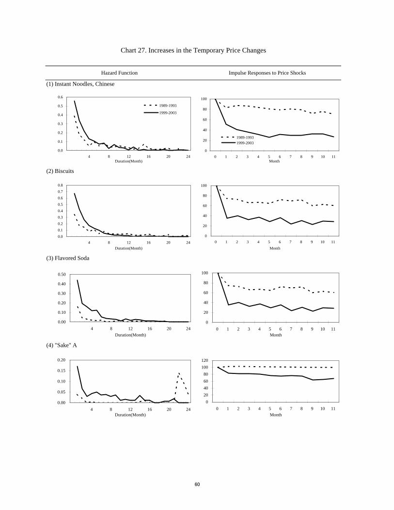
(1) Instant Noodles, Chinese

(2) Biscuits

(3) Flavored Soda

(4) "Sake" A

Chart 27. Increases in the Temporary Price Changes

Hazard Function Impulse Responses to Price Shocks

0.0

0.1

0.2

0.3

0.4

0.5

0.6

4 8 12 16 20 24Duration(Month)

1989-1993

1999-2003

0.00.10.20.30.40.50.60.70.8

4 8 12 16 20 24Duration(Month)

0.00

0.05

0.10

0.15

0.20

4 8 12 16 20 24Duration(Month)

020406080

100120

0 1 2 3 4 5 6 7 8 9 10 11Month

0

20

40

60

80

100

0 1 2 3 4 5 6 7 8 9 10 11Month

0.00

0.10

0.20

0.30

0.40

0.50

4 8 12 16 20 24Duration(Month)

0

20

40

60

80

100

0 1 2 3 4 5 6 7 8 9 10 11Month

1989-1993 1999-2003

0

20

40

60

80

100

0 1 2 3 4 5 6 7 8 9 10 11Month

60

(1) Fresh Food (2) Food Products

(3) Textiles (4) Other Industrial Products

(5) Public Services (6) General Services

Chart 28. Impulse Responses to Price Shocks

0

20

40

60

80

100

0 1 2 3 4 5 6 7 8 9 10 11

Month

CY1989-1993

CY1999-2003

(%)

0

20

40

60

80

100

0 1 2 3 4 5 6 7 8 9 10 11

Month

CY1989-1993

CY1999-2003

(%)

0

20

40

60

80

100

0 1 2 3 4 5 6 7 8 9 10 11

Month

CY1989-1993

CY1999-2003

(%)

0

20

40

60

80

100

0 1 2 3 4 5 6 7 8 9 10 11

Month

CY1989-1993

CY1999-2003

(%)

0

20

40

60

80

100

0 1 2 3 4 5 6 7 8 9 10 11

Month

CY1989-1993

CY1999-2003

(%)

0

20

40

60

80

100

0 1 2 3 4 5 6 7 8 9 10 11

Month

CY1989-1993

CY1999-2003

(%)

61