Embed Size (px)
Citation preview

18-2
Prelude
Ensuring equal service
I n 1984, in an effort to open the telecommunications market tocompetition, AT&T was split into eight regional companies. To
promote competition, more than one company was now allowed tooffer telecommunications services in a local market. But since it isn’t inthe public interest to have multiple companies digging up local streets tobury cables, one telephone company in each region is given responsibilityfor installing and maintaining all local lines and leasing capacity to othercarriers.
Each state’s Public Utilities Commission (PUC) is responsible for seeingthat there is fair access for all carriers. For example, the primary carriershould do repairs as quickly for customers of other carriers as for theirown. Significance tests are used to compare the levels of service. If a testindicates that service levels are not equivalent, the primary carrier pays apenalty.
PUCs and primary carriers perform many of these tests each day. Giventhe large amounts of money at stake, the significance tests described inearlier chapters are not sufficiently accurate. Instead, primary carriers likeVerizon have turned to resampling methods in an effort to achieve accurate
test results that provide a strong defense in an adversarial hearingbefore a PUC.
The resampling methods of this chapter providealternatives to the methods of earlier chapters for
finding standard errors and confidence intervalsand for performing significance tests.
18
Bootstrap Methodsand Permutation Tests
18.1 Why Resampling?
18.2 Introduction to Bootstrapping
18.3 Bootstrap Distributions andStandard Errors
18.4 How Accurate Is a BootstrapDistribution?
18.5 Bootstrap Confidence Intervals
18.6 Significance Testing UsingPermutation Tests
CH
AP
TER
18
Bootstrap Methodsand Permutation Tests

Bootstrap Methods and Permutation Tests18-4 CHAPTER 18 �
�
�
�
�
18.1 Why Resampling?
Fewer assumptions.
Greater accuracy.
Generality.
Promote understanding.
Statistics is changing. Modern computers and software make it possible tolook at data graphically and numerically in ways previously inconceivable.They let us do more realistic, accurate, and informative analyses than canbe done with pencil and paper.
The bootstrap, permutation tests, and other resampling methods are partof this revolution. Resampling methods allow us to quantify uncertaintyby calculating standard errors and confidence intervals and performingsignificance tests. They require fewer assumptions than traditional methodsand generally give more accurate answers (sometimes very much moreaccurate). Moreover, resampling lets us tackle new inference settings easily.For example, Chapter 7 presented methods for inference about the differencebetween two population means. But suppose you are really interested in a
of means, such as the ratio of average men’s salary to average women’ssalary. There is no simple traditional method for inference in this newsetting. Resampling not only works, but works in the same way as forthe difference in means. We don’t need to learn new formulas for everynew problem.
Resampling also helps us understand the concepts of statistical inference.The sampling distribution is an abstract idea. The bootstrap analog (the“bootstrap distribution”) is a concrete set of numbers that we analyze usingfamiliar tools like histograms. The standard deviation of that distributionis a concrete analog to the abstract concept of a standard error. Resam-pling methods for significance tests have the same advantage; permutationtests produce a concrete set of numbers whose “permutation distribution”approximates the sampling distribution under the null hypothesis. Compar-ing our statistic to these numbers helps us understand -values. Here is asummary of the advantages of these new methods:
For example, resampling methods do not require thatdistributions be Normal or that sample sizes be large.
Permutation tests, and some bootstrap methods, aremore accurate in practice than classical methods.
Resampling methods are remarkably similar for a wide rangeof statistics and do not require new formulas for every statistic. You donot need to memorize or look up special formulas for each procedure.
Bootstrap procedures build intuition by provid-ing concrete analogies to theoretical concepts.
Resampling has revolutionized the range of problems accessible to busi-ness people, statisticians, and students. It is beginning to revolutionize ourstandards of what is acceptable accuracy in high-stakes situations such aslegal cases, business decisions, and clinical trials.
ratio
P

18.2 Introduction to Bootstrapping 18-5
18.2 Introduction to Bootstrapping
Note on software
TELECOMMUNICATION REPAIR TIMES
elms03.e-academy.com/splus/
www.insightful.com/Hesterberg/bootstrap www.whfreeman.com
www.whfreeman.com
�
�
1
2
3
Bootstrapping and permutation tests are feasible only with the use ofsoftware to automate the heavy computation that these resampling methodsrequire. If you are sufficiently expert in programming or with a spreadsheet,you can program basic resampling methods yourself. But it is easier to usesoftware with resampling methods built in.
This chapter uses S-PLUS, the software choice of most statisticians do-ing research on resampling methods. A free student version of this softwareis available to students and faculty at .In addition, a student library containing data sets specifically for your book,menu-driven access to capabilities you’ll need, and a manual that accom-panies this chapter can be found at
or at . You may also order an S-PLUSmanual to supplement this book from .
Let’s get a feel for bootstrapping by seeing how it works in a specificexample. We’ll begin by showing how to bootstrap and then relate theresults to ideas you’ve already encountered, such as standard errors andsampling distributions.
Verizon is the primary local telephone company (the legal term is IncumbentLocal Exchange Carrier, ILEC) for a large area in the eastern United States.As such, it is responsible for providing repair service for the customers ofother telephone companies (known as Competing Local Exchange Carriers,CLECs) in this region. Verizon is subject to fines if the repair times (thetime it takes to fix a problem) for CLEC customers are substantially worsethan those for Verizon’s own customers. This is determined using hypothesistests, negotiated with the local Public Utilities Commission (PUC).
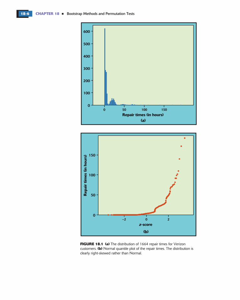
Webeginouranalysisby focusingonVerizon’sowncustomers. Figure18.1shows the distribution of a random sample of 1664 repair times. The datafile is . A quick glance at the distribution reveals that the data arefar from Normal. The distribution has a long right tail (skewness to the right).
The mean repair time for Verizon customers in this sample is 8 41hours. This is a statistic from just one random sample (albeit a fairly largeone). The statistic will vary if we take more samples, and its trustworthinessas an estimator of the population mean depends on how much it variesfrom sample to sample.
verizon.dat
x .
x
CA
SE18
.1
0
Repair times (in hours)
z-score
Rep
air
tim
es (
in h
ours
)
600
500
400
300
200
100
050 100 150
–2
150
100
50
00 2
(a)
(b)
Bootstrap Methods and Permutation Tests18-6 CHAPTER 18
FIGURE 18.1 (a)(b)
�
The distribution of 1664 repair times for Verizoncustomers. Normal quantile plot of the repair times. The distribution isclearly right-skewed rather than Normal.
1.57 0.22 19.67 0.00 0.22 3.12mean = 4.13
0.00 2.20 2.20 2.20 19.67 1.57mean = 4.64
3.12 0.00 1.57 19.67 0.22 2.20 mean = 4.46
0.22 3.12 1.57 3.12 2.20 0.22mean = 1.74
18.2 Introduction to Bootstrapping 18-7
FIGURE 18.2
Procedure for bootstrapping
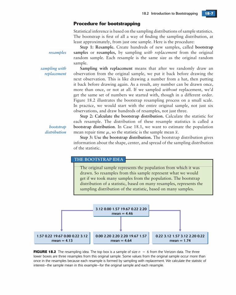
The resampling idea. The top box is a sample of size 6 from the Verizon data. The threelower boxes are three resamples from this original sample. Some values from the original sample occur more thanonce in the resamples because each resample is formed by sampling with replacement. We calculate the statistic ofinterest—the sample mean in this example—for the original sample and each resample.
n
Step 1: Resample. bootstrapsamples resamples,
Sampling with replacement
Step 2: Calculate the bootstrap distribution.
bootstrap distribution
Step 3: Use the bootstrap distribution.
THE BOOTSTRAP IDEA
�
�
resamples
sampling withreplacement
bootstrapdistribution
Statistical inference is based on the sampling distributions of sample statistics.The bootstrap is first of all a way of finding the sampling distribution, atleast approximately, from just one sample. Here is the procedure:
Create hundreds of new samples, calledor by sampling from the original
random sample. Each resample is the same size as the original randomsample.
means that after we randomly draw anobservation from the original sample, we put it back before drawing thenext observation. This is like drawing a number from a hat, then puttingit back before drawing again. As a result, any number can be drawn once,more than once, or not at all. If we sampled replacement, we’dget the same set of numbers we started with, though in a different order.Figure 18.2 illustrates the bootstrap resampling process on a small scale.In practice, we would start with the entire original sample, not just sixobservations, and draw hundreds of resamples, not just three.
Calculate the statistic foreach resample. The distribution of these resample statistics is called a
. In Case 18.1, we want to estimate the populationmean repair time , so the statistic is the sample mean .
The bootstrap distribution givesinformation about the shape, center, and spread of the sampling distributionof the statistic.
The original sample represents the population from which it wasdrawn. So resamples from this sample represent what we wouldget if we took many samples from the population. The bootstrapdistribution of a statistic, based on many resamples, represents thesampling distribution of the statistic, based on many samples.
with replacement
without
x
Bootstrap Methods and Permutation Tests18-8 CHAPTER 18
Bootstrap distribution for mean repair time
Bootstrap standard error for mean repair time
EXAMPLE 18.1
EXAMPLE 18.2
�
BOOTSTRAP STANDARD ERROR
bootstrap standard error
, x
Shape:
Center:
Spread:
��, x � �� �� � �
�
� �
�2
boot
�boot
The of a statistic is the standard deviationof the bootstrap distribution of that statistic.
If the statistic of interest is the sample mean , the bootstrap standarderror based on resamples is
1 1SE
1
In this expression, is the mean value of an individual resample. Thebootstrap standard error is just the ordinary standard deviation of thevalues of . The asterisk in distinguishes the mean of a resample fromthe mean of the original sample.
xn
x x
x
.x
xB
x xB B
xB
x xx
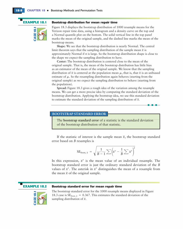
Figure 18.3 displays the bootstrap distribution of 1000 resample means for theVerizon repair time data, using a histogram and a density curve on the top anda Normal quantile plot on the bottom. The solid vertical line in the top panelmarks the mean of the original sample, and the dashed line marks the mean of thebootstrap means.
We see that the bootstrap distribution is nearly Normal. The centrallimit theorem says that the sampling distribution of the sample mean isapproximately Normal if is large. So the bootstrap distribution shape is close tothe shape we expect the sampling distribution to have.
The bootstrap distribution is centered close to the mean of theoriginal sample. That is, the mean of the bootstrap distribution has little biasas an estimator of the mean of the original sample. We know that the samplingdistribution of is centered at the population mean , that is, that is an unbiasedestimate of . So the resampling distribution again behaves (starting from theoriginal sample) as we expect the sampling distribution to behave (starting fromthe population).
Figure 18.3 gives a rough idea of the variation among the resamplemeans. We can get a more precise idea by computing the standard deviation of thebootstrap distribution. Applying the bootstrap idea, we use this standard deviationto estimate the standard deviation of the sampling distribution of .
The bootstrap standard error for the 1000 resample means displayed in Figure18.3 case is SE 0 367. This estimates the standard deviation of thesampling distribution of .
�
�
CA
SE18
.1C
ASE
18.1
7.5 8.0 8.5 9.0 9.5
Mean repair times of resamples (in hours)
(a)
ObservedMean
7.5
8.0
8.5
9.0
9.5
Mea
n re
pair
tim
es o
f re
sam
ples
(in
hou
rs)
–2 0 2z-score
(b)
18.2 Introduction to Bootstrapping 18-9
FIGURE 18.3 The bootstrap distribution for 1000 resamplemeans from the Verizon ILEC sample. The solid line in the toppanel marks the original sample mean, and the dashed line marksthe average of the bootstrap means. The Normal quantile plotconfirms that the bootstrap distribution is nearly Normal in shape.

Bootstrap Methods and Permutation Tests18-10 CHAPTER 18 �
Using software
APPLY YOURKNOWLEDGE
Repeat 1000 times {Draw a resample with replacement from the data.Calculate the resample mean.Save the resample mean into a vector (a variable).
}Make a histogram and Normal quantile plot of the 1000 means.Calculate the standard deviation of the 1000 means.
18.1 Bootstrap a small data set by hand.
�
�
� �
�
�
� �
�
We know a great deal about the behavior of the sample mean in largesamples. Examples 18.1 and 18.2 verify the bootstrap idea for the mean ofa sample of size 1664. The examples show that the shape, bias, and spreadof the bootstrap distribution are close to the shape, bias, and spread of thesampling distribution.
. This fact is the basis of the usefulness ofbootstrap methods.
Software is essential for bootstrapping in practice. Here is an outline of theprogram you would write if your software will choose random samples froma set of data but does not have bootstrap functions:
x n
x s ns
s ..
n
with replacement
n
x
This is also true in many situations where we do notknow the sampling distribution
In fact, we know that the standard deviation of is , where is thestandard deviation of individual observations in the population. Our usualestimate of this quantity is the standard error of , , based on the standarddeviation of the original sample. In this example,
14 690 360
1664
The bootstrap standard error agrees quite closely with this formula-basedestimate.
To illustrate the bootstrapprocedure, let’s bootstrap a small random subset of the Verizondata:
3.12 0.00 1.57 19.67 0.22 2.20
(a) Sample from this initial SRS by rolling a die. Rollinga 1 means select the first member of the SRS, a 2 means select thesecond member, and so on. (You can also use Table B of randomdigits, responding only to digits 1 to 6.) Create 20 resamples ofsize 6.
(b) Calculate the sample mean for each of the resamples.
(c) Make a stemplot of the means of the 20 resamples. This is the bootstrapdistribution.
(d) Calculate the bootstrap standard error.
� �
CA
SE1
8.1
APPLY YOURKNOWLEDGE
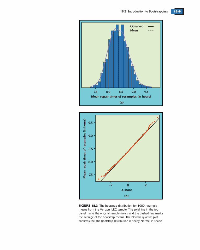
Number of Replications: 1000
Percentiles: 2.5% 5.0% 95.0% 97.5%mean 7.717 7.814 9.028 9.114
Summary Statistics:
meanObserved
8.412Mean8.395
SE0.3672
Bias–0.01698
18.2 Introduction to Bootstrapping 18-11
FIGURE 18.4
Using S-PLUSEXAMPLE 18.3
Why does bootstrapping work?
S-PLUSoutput for the Verizon databootstrap, Case 18.1.
APPLY YOURKNOWLEDGE
bootILEC = bootstrap(data = ILEC, statistic = mean)plot(bootILEC)qqnorm(bootILEC)summary(bootILEC)
bootILEC
summary ObservedMean
Bias MeanObserved SE
Percentiles
Observed
18.2 Earnings for white female hourly workers.
�
It might seem that the bootstrap creates data out of nothing. This seemssuspicious. But we are not using the resampled observations as if they werereal data—the bootstrap is not a substitute for gathering more data to
readdata.ssc
x .
Suppose that we save the 1664 Verizon repair times as the variable ILEC in S-PLUS(commands to do this are in the file ). We can make 1000 resamplesand analyze their means using these commands:
The same functions are available in menus, but it is a bit easier to discuss thetyped commands. The first command resamples from the ILEC data set, calculatesthe means of the resamples, and saves the bootstrap results as the object named
. By default, S-PLUS takes 1000 resamples. The remaining threecommands make a histogram (with a density curve) and a Normal quantile plotand calculate numerical summaries. The summaries include the bootstrap standarderror.
Figure 18.4 is part of the output of the command. Thecolumn gives the mean 8 412 of the original sample. is the mean ofthe resample means. The column shows the difference between theand the values. The bootstrap standard error is displayed in thecolumn. The are percentiles of the bootstrap distribution, thatis, of the means of the 1000 resamples pictured in Figure 18.3. All of these valuesexcept will differ a bit if you repeat 1000 resamples, because resamplesare drawn at random.
Bootstrap the mean ofthe white female hourly workers data from Table 1.8 (page 31).
(a) Plot the bootstrap distribution (histogram or density plot andNormal quantile plot). Is it approximately Normal?
(b) Find the bootstrap standard error.
(c) Find the 2.5th and 97.5th percentiles of the bootstrap distribution.
APPLY YOURKNOWLEDGE
CA
SE1
.2
CA
SE18
.1
Bootstrap Methods and Permutation Tests18-12 CHAPTER 18 �
Sampling distribution and bootstrap distribution
THE PLUG-IN PRINCIPLE
��
�
�
�
� �
�
�
� �
improve accuracy. Instead, the bootstrap idea is to use the resample means toestimate how the sample mean of a sample of size 1664 from this populationvaries because of random sampling.
Using the data twice—once to estimate the population mean, and againto estimate the variation in the sample mean—is perfectly legitimate. Indeed,we’ve done this many times before: for example, when we calculated bothand from the same data. What is different is that
1. we compute a standard error by using resampling rather than the formula, and
2. we use the bootstrap distribution to see whether the sampling distributionis approximately Normal, rather than just hoping that our sample is largeenough for the central limit theorem to apply.
The bootstrap idea applies to statistics other than sample means. To usethe bootstrap more generally, we appeal to another principle—one that wehave often applied without thinking about it.
To estimate a parameter, a quantity that describes the population,use the statistic that is the corresponding quantity for the sample.
The plug-in principle suggests that we estimate a population meanby the sample mean and a population standard deviation by thesample standard deviation . Estimate a population median by the samplemedian. To estimate the standard deviation of the sample mean for an SRS,
, plug in to get . The bootstrap idea itself is a form of theplug-in principle: substitute the distribution of the data for the populationdistribution, then draw samples (resamples) to mimic the process of buildinga sampling distribution. Let’s look at this more closely.
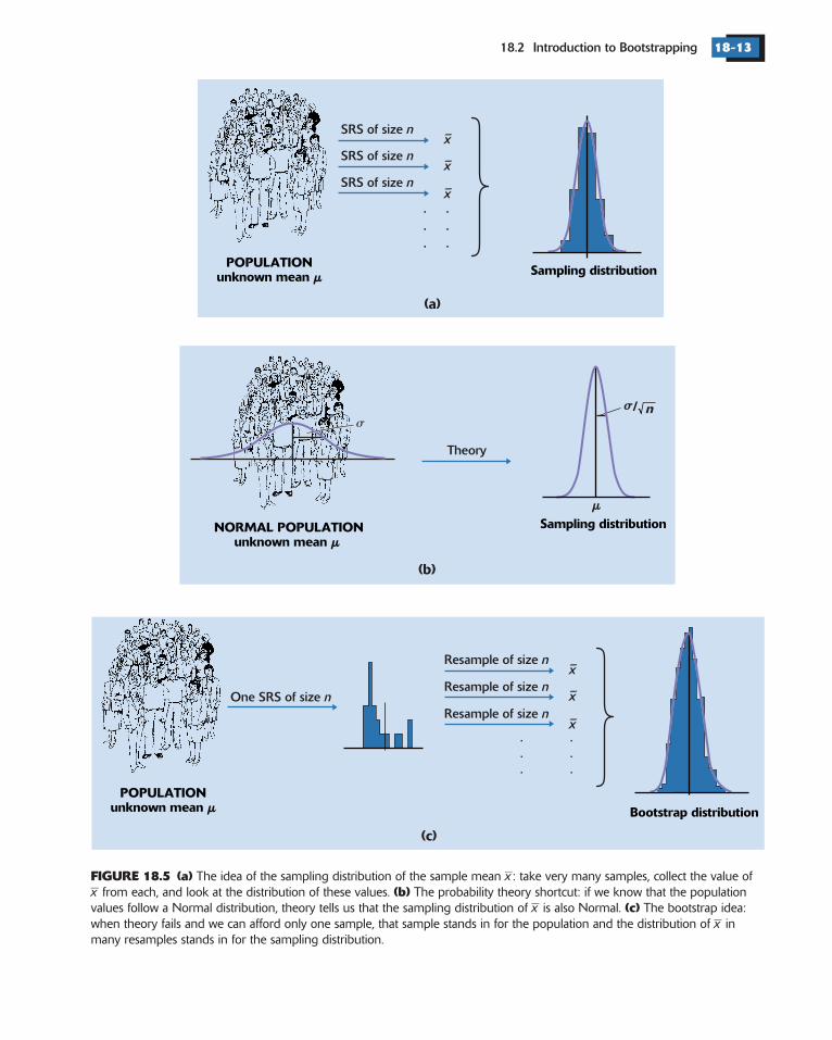
Confidence intervals, hypothesis tests, and standard errors are all based onthe idea of the of a statistic—the distribution of valuestaken by the statistic in all possible samples of the same size from the samepopulation. Figure 18.5(a) shows the idea of the sampling distribution of thesample mean . In practice, we can’t take a large number of random samplesin order to construct this sampling distribution. Instead, we have used ashortcut: if we start with a model for the distribution of the population, thelaws of probability tell us (in some situations) what the sampling distributionis. Figure 18.5(b) illustrates an important situation in which this approachworks. If the population has a Normal distribution, then the samplingdistribution of is also Normal.
In many settings, we have no model for the population. We then can’tappeal to probability theory, and we also can’t afford to actually take manysamples. The bootstrap rescues us. Use the one sample we have as thoughit were the population, taking many resamples from it to construct the
xs n
s n
xs
n s s n
sampling distribution
x
x
(b)
Theory
Sampling distribution NORMAL POPULATIONunknown mean �
�
�
�
n/�
Resample of size n
Resample of size n
Resample of size n
(c)
One SRS of size n
Bootstrap distributionPOPULATION
unknown mean �
x–
x–
x–
···
···
SRS of size n
(a)
SRS of size n
SRS of size n
Sampling distributionPOPULATION
unknown mean �
x–
x–
x–
···
···
18.2 Introduction to Bootstrapping 18-13
FIGURE 18.5 (a)(b)
(c)
The idea of the sampling distribution of the sample mean : take very many samples, collect the value offrom each, and look at the distribution of these values. The probability theory shortcut: if we know that the population
values follow a Normal distribution, theory tells us that the sampling distribution of is also Normal. The bootstrap idea:when theory fails and we can afford only one sample, that sample stands in for the population and the distribution of inmany resamples stands in for the sampling distribution.
xx
xx
Bootstrap Methods and Permutation Tests18-14 CHAPTER 18
ECTION UMMARY
ECTION XERCISES
�
�
�
�
�
�
S
S
18.2 S
18.2 E
resamplesbootstrap distribution
plug-in principle
bootstrap standard error
bootstrap distribution. Figure 18.5(c) outlines the process. Then usethe bootstrap distribution in place of the sampling distribution.
In practice, it is usually impractical to actually draw all possible resam-ples. We carry out the bootstrap idea by using 1000 or so randomly chosenresamples. We could directly estimate the sampling distribution by choosing1000 samples of the same size from the original population, as Figure 18.5(a)illustrates. But it is very much faster and cheaper to let software resamplefrom the original sample than to select many samples from the population.Even if we have a large budget, we would prefer to spend it on obtaininga single larger sample rather than many smaller samples. A larger samplegives a more precise estimate.
In most cases, the bootstrap distribution has approximately the sameshape and spread as the sampling distribution, but it is centered at the originalstatistic value rather than the parameter value. The bootstrap allows us tocalculate standard errors for statistics for which we don’t have formulas andto check Normality for statistics that theory doesn’t easily handle. We’ll dothis in the next section.
To bootstrap a statistic (for example, the sample mean), draw hundredsof with replacement from the original sample data, calculate thestatistic for each resample, and inspect the of theresampled statistics.
The bootstrap distribution approximates the sampling distribution of thestatistic. This is an example of the : use a quantity basedon the sample to approximate a similar quantity from the population.
Bootstrap distributions usually have approximately the same shapeand spread as the sampling distribution but are centered at the statistic(from the original data) when the sampling distribution is centered at theparameter (of the population).
Use graphs and numerical summaries to determine whether the bootstrapdistribution is approximately Normal and centered at the original statisticand to get an idea of its spread. The is thestandard deviation of the bootstrap distribution.
The bootstrap does not replace or add to the original data. We use thebootstrap distribution as a way to estimate the variation in a statistic basedon the original data.
Unless an exercise instructs you otherwise, use 1000 resamples for all bootstrapexercises. S-PLUS uses 1000 resamples unless you ask for a different number. Alwayssave your bootstrap results in a file or S-PLUS object, as in Example 8.3, so thatyou can use them again later.
18.2 Introduction to Bootstrapping 18-15
18.3 Spending by shoppers.
18.4 Guinea pig survival times.
18.5 More on supermarket shoppers.
�
�
4
xn
xn
x
Here are the dollar amounts spent by 50 consecutiveshoppers at a supermarket. We are willing to regard this as an SRS of allshoppers at this market.
3.11 8.88 9.26 10.81 12.69 13.78 15.23 15.62 17.00 17.3918.36 18.43 19.27 19.50 19.54 20.16 20.59 22.22 23.04 24.4724.58 25.13 26.24 26.26 27.65 28.06 28.08 28.38 32.03 34.9836.37 38.64 39.16 41.02 42.97 44.08 44.67 45.40 46.69 48.6550.39 52.75 54.80 59.07 61.22 70.32 82.70 85.76 86.37 93.34
(a) Make a histogram of the data. The distribution is slightly skewed.
(b) The central limit theorem says that the sampling distribution of the sam-ple mean becomes Normal as the sample size increases. Is the samplingdistribution roughly Normal for 50? To find out, bootstrap thesedata and inspect the bootstrap distribution of the mean.
The lifetimes of machines before a breakdownand the survival times of cancer patients after treatment are typically stronglyright-skewed. Here are the survival times (in days) of 72 guinea pigs in amedical trial:
43 45 53 56 56 57 58 66 67 7374 79 80 80 81 81 81 82 83 8384 88 89 91 91 92 92 97 99 99
100 100 101 102 102 102 103 104 107 108109 113 114 118 121 123 126 128 137 138139 144 145 147 156 162 174 178 179 184191 198 211 214 243 249 329 380 403 511522 598
(a) Make a histogram of the survival times. The distribution is stronglyskewed.
(b) The central limit theorem says that the sampling distribution of the sam-ple mean becomes Normal as the sample size increases. Is the samplingdistribution roughly Normal for 72? To find out, bootstrap thesedata and inspect the bootstrap distribution of the mean (use a Normalquantile plot). How does the distribution differ from Normality? Is thebootstrap distribution more or less skewed than the data distribution?
Here is an SRS of 10 of the amounts spentfrom Exercise 18.3:
18.43 52.75 50.39 34.98 19.27 19.54 15.23 17.39 12.69 93.34
We expect the sampling distribution of to be less close to Normal forsamples of size 10 than for samples of size 50 from a skewed distribution.This sample includes a high outlier.
(a) Create and inspect the bootstrap distribution of the sample mean fromthese data. Is it less close to Normal than your distribution from Exercise18.3?
Bootstrap Methods and Permutation Tests18-16 CHAPTER 18 �
18.3 Bootstrap Distributionsand Standard Errors
BIAS
biased
18.6 More on survival times.
18.7 Comparing standard errors.�
�
�
�
In this section we’ll use the bootstrap procedure to find bootstrap distribu-tions and standard errors for statistics other than the mean. The shape of thebootstrap distribution approximates the shape of the sampling distribution,so we can use the bootstrap distribution to check Normality of the samplingdistribution. If the sampling distribution appears to be Normal and centeredat the true parameter value, we can use the bootstrap standard error tocalculate a confidence interval. So we need to use the bootstrap to checkthe center of the sampling distribution as well as the shape and spread. Itturns out that the bootstrap does not reveal the center directly, but ratherreveals the .
A statistic used to estimate a parameter is when its samplingdistribution is not centered at the true value of the parameter. Thebias of a statistic is the mean of the sampling distribution minus theparameter.
The bootstrap method allows us to check for bias by seeing whetherthe bootstrap distribution of a statistic is centered at the statistic ofthe original random sample. The bootstrap estimate of bias is themean of the bootstrap distribution minus the statistic for the originaldata.
x
x s ns
s n
t
bias
(b) Compare the bootstrap standard errors for your two runs. What ac-counts for the larger standard error for the smaller sample?
Here is an SRS of 20 of the guinea pig survivaltimes from Exercise 18.4:
92 123 88 598 100 114 89 522 58 191137 100 403 144 184 102 83 126 53 79
We expect the sampling distribution of to be less close to Normal forsamples of size 20 than for samples of size 72 from a skewed distribution.These data include some extreme high outliers.
(a) Create and inspect the bootstrap distribution of the sample mean forthese data. Is it less close to Normal than your distribution from Exercise18.4?
(b) Compare the bootstrap standard errors for your two runs. What ac-counts for the larger standard error for the smaller sample?
We have two ways to estimate the standarddeviation of a sample mean : use the formula for the standard erroror use the bootstrap standard error. Find the sample standard deviationfor the 50 amounts spent in Exercise 18.3 and use it to find the standarderror of the sample mean. How closely does your result agree with thebootstrap standard error from your resampling in Exercise 18.3?

18.3 Bootstrap Distributions and Standard Errors 18-17
Bootstrapping the mean selling priceEXAMPLE 18.4
REAL ESTATE SALE PRICES
5
We are interested in the sales prices of residential property in Seattle. Un-fortunately, the data available from the county assessor’s office do notdistinguish residential property from commercial property. Most of the salesin the assessor’s records are residential, but a few large commercialsales in a sample can greatly increase the mean selling price. We preferto use a measure of center that is more resistant than the mean. When we dothis, we know less about the sampling distribution than if we used the meanto measure center. The bootstrap is very handy in such settings.
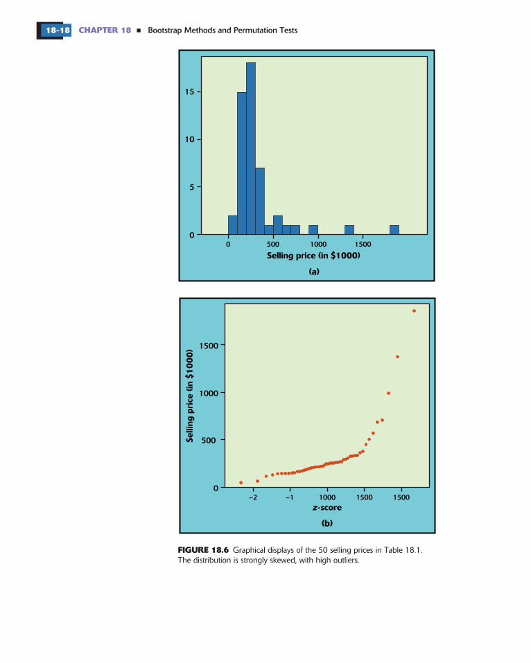
Table 18.1 gives the selling prices for a random sample (SRS of size 50)from the population of all 2002 Seattle real estate sales, as recorded by thecounty assessor. The sales include houses, condominiums, and commercialreal estate but exclude plots of undeveloped land.
Figure 18.6 describes these data with a histogram and Normal quantileplot. As we expect, the distribution is strongly skewed to the right. Thereare several high outliers, which may be commercial sales.
x
x
x
142 232 132.5 200 362 244.95 335 324.5 222 225175 50 215 260 307 210.95 1370 215.5 179.8 217197.5 146.5 116.7 449.9 266 265 256 684.5 257 570149.4 155 244.9 66.407 166 296 148.5 270 252.95 507705 1850 290 164.95 375 335 987.5 330 149.95 190
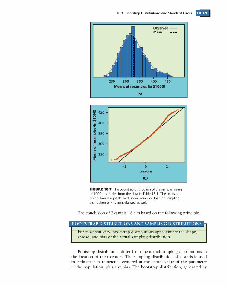
The skewness of the distribution of real estate prices affects the samplingdistribution of the sample mean. We cannot see the sampling distribution directlywithout taking many samples, but the bootstrap distribution gives us a clue.Figure 18.7 shows the bootstrap distribution of the sample mean based on1000 resamples from the data in Table 18.1. The distribution is skewed to theright—that is, a sample of size 50 is not large enough to allow us to act as if hasa Normal distribution.
There is some good news as well. The bootstrap distribution shows thatthe outliers do not cause large bias—the mean of the bootstrap distribution isapproximately equal to the sample mean of the data in Table 18.1 (the solidand dotted lines nearly coincide). We conclude that the sampling distribution isskewed but has small bias. This isn’t surprising: we know that is an unbiasedestimator of the population mean , whether or not the population has a Normaldistribution.
�
CA
SE18.2
CA
SE18
.2
TABLE 18.1 Selling prices (in $1000) for an SRS of 50 Seattle real estatesales in 2002
z-score
(b)
0
Selling price (in $1000)
Selli
ng p
rice
(in
$1
00
0)
500 1000 1500
(a)
0
5
10
15
–2 –1 1000 1500 15000
500
1000
1500
Bootstrap Methods and Permutation Tests18-18 CHAPTER 18
FIGURE 18.6
�
Graphical displays of the 50 selling prices in Table 18.1.The distribution is strongly skewed, with high outliers.
250 300 350 400 450Means of resamples (in $1000)
250
300
350
400
450
–2 0 2z-score
Mea
ns o
f re
sam
ples
(in
$1
00
0)
(a)
(b)
ObservedMean
18.3 Bootstrap Distributions and Standard Errors 18-19
FIGURE 18.7 The bootstrap distribution of the sample meansof 1000 resamples from the data in Table 18.1. The bootstrapdistribution is right-skewed, so we conclude that the samplingdistribution of is right-skewed as well.x
BOOTSTRAP DISTRIBUTIONS AND SAMPLING DISTRIBUTIONS
The conclusion of Example 18.4 is based on the following principle.
For most statistics, bootstrap distributions approximate the shape,spread, and bias of the actual sampling distribution.
Bootstrap distributions differ from the actual sampling distributions inthe location of their centers. The sampling distribution of a statistic usedto estimate a parameter is centered at the actual value of the parameterin the population, plus any bias. The bootstrap distribution, generated by
Bootstrap Methods and Permutation Tests18-20 CHAPTER 18
25% trimmed mean for the real estate dataEXAMPLE 18.5
�
Bootstrap distributions of other statistics
APPLY YOURKNOWLEDGE
TRIMMED MEAN
trimmed mean
18.8 Supermarket shoppers.
18.9 Guinea pig survival.
25%
resampling from a single sample, is centered at the value of the statistic forthe original sample, plus any bias. The two biases are similar even thoughthe two centers are not.
In estimating the center of Seattle real estate prices, we cannot act as ifthe sampling distribution of were Normal. We have two alternatives: usea confidence interval not based on Normality or choose a measure of centerwhose distribution is closer to Normal. We will see that advanced bootstrapmethods do produce confidence intervals not based on Normality. For now,however, we choose to bootstrap a different statistic that is more resistantto skewness and outliers.
One statistic we might consider in place of the mean is the median. Here,instead, we’ll use a .
A is the mean of only the center observations in adata set. In particular, the 25% trimmed mean ignores thesmallest 25% and the largest 25% of the observations. It is the meanof the middle 50% of the observations.
Recall that the median is the mean of the 1 or 2 middle observations.The trimmed mean often does a better job of representing the average oftypical observations than does the median. Bootstrapping trimmed meansalso works better than bootstrapping medians, because the bootstrap doesn’twork well for statistics that depend on only 1 or 2 observations.
x
x
x
25% trimmed mean
x
What is the bootstrap estimate of the bias fromyour resamples in Exercise 18.3? What does this tell you about the biasencountered in using to estimate the mean spending for all shoppers at thismarket?
What is the bootstrap estimate of the bias from yourresamples in Exercise 18.4? What does this tell you about the bias encoun-tered in using to estimate the mean survival time for all guinea pigs thatreceive the same experimental treatment?
We don’t need any distribution facts about the trimmed mean to use the bootstrap.We bootstrap the 25% trimmed mean just as we bootstrapped the sample mean:draw 1000 resamples, calculate the 25% trimmed mean for each resample, andform the bootstrap distribution from these 1000 values. Figure 18.8 shows theresult.
Comparing Figures 18.7 and 18.8 shows that the bootstrap distribution of thetrimmed mean is less skewed than the bootstrap distribution of the mean and iscloser to Normal. It is close enough that we will calculate a confidence interval forthe population trimmed mean based on Normality. (If high accuracy were
CA
SE18
.2
APPLY YOURKNOWLEDGE

200 220 240 260 280 300Means of resamples (in $1000)
Den
sity
200
220
240
260
280
–2 0 2z-score
Mea
ns o
f re
sam
ples
(in
$1
00
0)
(a)
(b)
ObservedMean
18.3 Bootstrap Distributions and Standard Errors 18-21
FIGURE 18.8 The bootstrap distribution of the 25% trimmedmeans of 1000 resamples from the data in Table 18.1. Thebootstrap distribution is roughly Normal.
Number of Replications: 1000
Summary Statistics:Observed Mean Bias SE
TrimMean 244 244.7 0.7171 16.83
important, we would prefer one of the more accurate confidence intervalprocedures we discuss later.)
The distribution of the trimmed mean is also narrower than that of the mean.For a long-tailed distribution such as this, the 25% trimmed mean is a less variableestimate of the center of the population than is the ordinary mean. Here is thesummary output from S-PLUS:

Bootstrap Methods and Permutation Tests18-22 CHAPTER 18
Bootstrap confidence interval for the trimmed meanEXAMPLE 18.6
�
Bootstrap confidence intervalst
t
BOOTSTRAP CONFIDENCE INTERVAL
, x
, x
t tt
�
�
�
�
,
� �
�
��
�
�
�
�
�
�
� �
There is another “bootstrap confidence interval” in common use. It estimates the value of thatis appropriate for the data rather than using a value from a table.
boot statistic
�
�
�
�
�
�
�
�
�
25%
25%
boot
25% boot
Recall the familiar one-sample confidence interval (page 435) for the meanof a Normal population,
This interval is based on the Normal sampling distribution of the samplemean and the formula for the standard error of .
When a bootstrap distribution is approximately Normal and has smallbias, we can use essentially the same recipe with the bootstrap standarderror to get a confidence interval for any parameter.
Suppose that the bootstrap distribution of a statistic from an SRSof size is approximately Normal and that the bias is small. Anapproximate level confidence interval for the parameter thatcorresponds to this statistic by the plug-in principle is
statistic SE
where is the critical value of the ( 1) distribution with areabetween and .
25%
25%
x
n
x.
x t . .
.
. , .
nt .
t
sx t
n
x s n x
nC
t
t t n Ct t
The trimmed mean for the sample is 244, the mean of the 1000 trimmedmeans of the resamples is 244.7, and the bootstrap standard error is 16.83.
We want to estimate the 25% trimmed mean of the population of all 2002Seattle real estate selling prices. Table 18.1 gives an SRS of size 50.The software output in Example 18.5 shows that the trimmed mean of thissample is 244 and that the bootstrap standard error of this statistic isSE 16 83. A 95% confidence interval for the population trimmed meanis therefore
SE 244 (2 009)(16 83)
244 33 81
(210 19 277 81)
Because Table D does not have entries for 1 49 degrees of freedom, we used2 009, the entry for 50 degrees of freedom.
We are 95% confident that the 25% trimmed mean (the mean of the middle50%) for the population of real estate sales in Seattle in 2002 is between $210,190and $277,810.
t
� �
�
�
CA
SE18
.2
18.3 Bootstrap Distributions and Standard Errors 18-23
Bootstrapping to compare two groups
APPLY YOURKNOWLEDGE
BOOTSTRAP FOR COMPARING TWO POPULATIONS
18.10 Confidence interval for shoppers’ mean spending.
18.11 Trimmed mean for shoppers’ spending.
18.12 Median for shoppers’ spending.
Two-sample problems (Section 7.2) are among the most common statisticalsettings. In a two-sample problem, we wish to compare two populations,such as male and female customers, based on separate samples from eachpopulation. When both populations are roughly Normal, the two-sample
procedures compare the two population means. The bootstrap can alsocompare two populations, without the Normality condition and withoutthe restriction to comparison of means. The most important new idea isthat bootstrap resampling must mimic the “separate samples” design thatproduced the original data.
Given independent SRSs of sizes and from two populations:
1. Draw a resample of size with replacement from the first sampleand a separate resample of size from the second sample.Compute a statistic that compares the two groups, such as thedifference between the two sample means.
2. Repeat this resampling process hundreds of times.
3. Construct the bootstrap distribution of the statistic. Inspect itsshape, bias, and bootstrap standard error in the usual way.
t
t
t
t
t
n m
nm
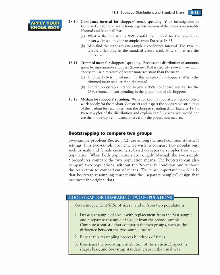
Your investigation inExercise 18.3 found that the bootstrap distribution of the mean is reasonablyNormal and has small bias.
(a) What is the bootstrap 95% confidence interval for the populationmean , based on your resamples from Exercise 18.3?
(b) Also find the standard one-sample confidence interval. The two in-tervals differ only in the standard errors used. How similar are theintervals?
Because the distribution of amountsspent by supermarket shoppers (Exercise 18.3) is strongly skewed, we mightchoose to use a measure of center more resistant than the mean.
(a) Find the 25% trimmed mean for this sample of 50 shoppers. Why is thetrimmed mean smaller than the mean?
(b) Use the bootstrap method to give a 95% confidence interval for the25% trimmed mean spending in the population of all shoppers.
We remarked that bootstrap methods oftenwork poorly for the median. Construct and inspect the bootstrap distributionof the median for resamples from the shopper spending data (Exercise 18.3).Present a plot of the distribution and explain carefully why you would notuse the bootstrap confidence interval for the population median.
�
APPLY YOURKNOWLEDGE

Bootstrap Methods and Permutation Tests18-24 CHAPTER 18
Service times in telecommunicationsEXAMPLE 18.7
�
Number of Replications: 1000
Summary Statistics:Observed Mean Bias SE
meanDiff -8.098 -8.251 -0.1534 4.052
Service provider
�
�
�
� �
n x s
1 2
1 2
1 2
In the setting of Example 18.7 we want to estimate the difference ofpopulation means, , but we are reluctant to use the two-sample
confidence interval because one of the samples is both quite small andvery skewed. To compute the bootstrap standard error for the difference insample means , resample separately from the two samples. Each of our1000 resamples consists of two group resamples, one of size 1664 drawnwith replacement from the Verizon data and one of size 23 drawn withreplacement from the CLEC data. For each combined resample, computethe statistic . The 1000 differences form the bootstrap distribution.The bootstrap standard error is the standard deviation of the bootstrapdistribution. Here is the S-PLUS output:
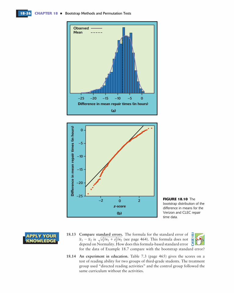
The bootstrap distribution and Normal quantile plot are shown in Figure18.10. The bootstrap distribution is not close to Normal. It has a short righttail and a long left tail, so that it is skewed to the left. We are unwilling to usea bootstrap confidence interval. That is, no method based on Normalityis safe. In Section 18.5, we will see that there are other ways of using thebootstrap to get confidence intervals that can be safely used in this andsimilar examples.
t
x x
x x
t
Incumbent local exchange carriers (ILECs), such as Verizon, install and maintainlocal telephone lines, lease capacity, and perform repairs for the competing localexchange carriers (CLECs). Figure 18.9 shows density curves and Normal quantileplots for the repair times (in hours) of 1664 service requests from customers ofVerizon and 23 requests from customers of a CLEC during the same time period.The distributions are both far from Normal. Here are some summarystatistics:
Verizon 1664 8.4 14.7CLEC 23 16.5 19.5Difference 8.1
The data suggest that repair times may be longer for the CLEC. The mean repairtime, for example, is almost twice as long for CLEC customers as for Verizoncustomers.
�
CA
SE18
.1

Den
sity
ILECCLEC
ILECCLEC
n = 1664n = 23
150
100
50
0
0 50 100 150 200
Repair time (in hours)R
epai
r ti
me
(in h
ours
)
(a)
–2 0 2z-score
(b)
18.3 Bootstrap Distributions and Standard Errors 18-25
FIGURE 18.9 Comparing the distributions of repair times(in hours) for 1664 requests from Verizon customers and23 requests for customers of a CLEC. The top panel showsdensity curves and the bottom panel shows Normal quantileplots. (The density curves appear to show negative repairtimes—this is due to how the density curves are calculatedfrom data, not because any times are negative.)
0
–5
–10
–15
–20
–25
–25 –20 –15 –10 –5 0
Difference in mean repair times (in hours)
Diff
eren
ce in
mea
n re
pair
tim
es (
in h
ours
)
(a)
–2 0 2z-score
(b)
ObservedMean
Bootstrap Methods and Permutation Tests18-26 CHAPTER 18
FIGURE 18.10
�
Thebootstrap distribution of thedifference in means for theVerizon and CLEC repairtime data.
APPLY YOURKNOWLEDGE
18.13 Compare standard errors.
18.14 An experiment in education.
� �2 21 2 1 21 2x x s n s n
The formula for the standard error ofis / / (see page 464). This formula does not
depend on Normality. How does this formula-based standard errorfor the data of Example 18.7 compare with the bootstrap standard error?
Table 7.3 (page 465) gives the scores on atest of reading ability for two groups of third-grade students. The treatmentgroup used “directed reading activities” and the control group followed thesame curriculum without the activities.
�
CA
SE1
8.1
APPLY YOURKNOWLEDGE

18.3 Bootstrap Distributions and Standard Errors 18-27
EYOND THE ASICS: HE OOTSTRAP FORA CATTERPLOT MOOTHER
Do some lottery numbers pay more?EXAMPLE 18.8
B B T BS S
18.15 Healthy versus failed companies.
1 2
1 2
6
The bootstrap idea can be applied to quite complicated statistical methods,such as the scatterplot smooth illustrated in Chapter 2 (page 126).
The straight line in Figure 18.11 is the least-squares regression line. Theline shows a general trend of higher payoffs for larger winning numbers. Thecurve in the figure was fitted to the plot by a scatterplot smoother that followslocal patterns in the data rather than being constrained to a straight line.The curve suggests that there were larger payoffs for numbers in the intervals000 to 100, 400 to 500, 600 to 700, and 800 to 999. When people pick“random” numbers, they tend to choose numbers starting with 2, 3, 5, or 7,so these numbers have lower payoffs. This pattern disappeared after 1976—itappears that players noticed the pattern and changed their number choices.
Are the patterns displayed by the scatterplot smooth just chance? We canuse the bootstrap distribution of the smoother’s curve to get an idea of how
x x
t
t
x xt
t
t
(a) Bootstrap the difference in means and report the bootstrapstandard error.
(b) Inspect the bootstrap distribution. Is a bootstrap confidence intervalappropriate? If so, give the interval.
(c) Compare the bootstrap results with the two-sample confidence intervalreported on page 478.
Table 7.4 (page 476) containsthe ratio of current assets to current liabilities for random samplesof healthy firms and failed firms. Find the difference in means(healthy minus failed).
(a) Bootstrap the difference in means and look at the bootstrapdistribution. Does it meet the conditions for a bootstrap confidenceinterval?
(b) Report the bootstrap standard error and the bootstrap confidenceinterval.
(c) Compare the bootstrap results with the two-sample confidence intervalreported on page 479.
The New Jersey Pick-It Lottery is a daily numbers game run by the state of NewJersey. We’ll analyze the first 254 drawings after the lottery was started in 1975.Buying a ticket entitles a player to pick a number between 000 and 999. Half ofthe money bet each day goes into the prize pool. (The state takes the other half.)The state picks a winning number at random, and the prize pool is shared equallyamong all winning tickets.
Although all numbers are equally likely to win, numbers chosen by fewerpeople have bigger payoffs if they win because the prize is shared among fewertickets. Figure 18.11 is a scatterplot of the first 254 winning numbers and theirpayoffs. What patterns can we see?
�
�
CA
SE7
.2
200
400
600
800
0 200 400 600 800 1000
Number
Pay
off
SmoothRegression line
200
400
600
800
0 200 400 600 800 1000
Number
Pay
off
Original smoothBootstrap smooths
Bootstrap Methods and Permutation Tests18-28 CHAPTER 18
FIGURE 18.11
FIGURE 18.12
�
The first 254 winning numbers in the New Jersey Pick-ItLottery and the payoffs for each. To see patterns we use least-squaresregression ( ) and a scatterplot smoother ( ).
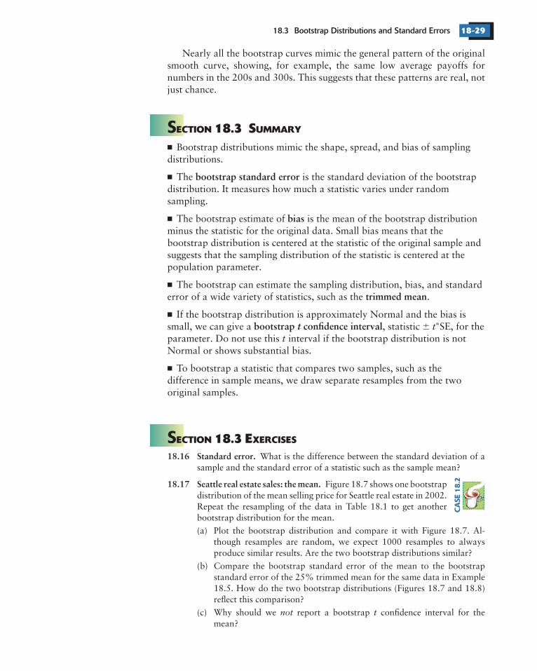
The curves produced by the scatterplot smoother for20 resamples from the data displayed in Figure 18.11. The curve for theoriginal sample is the heavy line.
line curve
much random variability there is in the curve. Each resample “statistic” isnow a curve rather than a single number. Figure 18.12 shows the curvesthat result from applying the smoother to 20 resamples from the 254 datapoints in Figure 18.11. The original curve is the thick line. The spread of theresample curves about the original curve shows the sampling variability ofthe output of the scatterplot smoother.
18.3 Bootstrap Distributions and Standard Errors 18-29
ECTION UMMARY
ECTION XERCISES
�
�
�
�
�
�
S
S
18.3 S
18.3 E
bootstrap standard error
bias
trimmed mean
bootstrap confidence interval
18.16 Standard error.
18.17 Seattle real estate sales: the mean.
� �
Nearly all the bootstrap curves mimic the general pattern of the originalsmooth curve, showing, for example, the same low average payoffs fornumbers in the 200s and 300s. This suggests that these patterns are real, notjust chance.
Bootstrap distributions mimic the shape, spread, and bias of samplingdistributions.
The is the standard deviation of the bootstrapdistribution. It measures how much a statistic varies under randomsampling.
The bootstrap estimate of is the mean of the bootstrap distributionminus the statistic for the original data. Small bias means that thebootstrap distribution is centered at the statistic of the original sample andsuggests that the sampling distribution of the statistic is centered at thepopulation parameter.
The bootstrap can estimate the sampling distribution, bias, and standarderror of a wide variety of statistics, such as the .
If the bootstrap distribution is approximately Normal and the bias issmall, we can give a , statistic SE, for theparameter. Do not use this interval if the bootstrap distribution is notNormal or shows substantial bias.
To bootstrap a statistic that compares two samples, such as thedifference in sample means, we draw separate resamples from the twooriginal samples.
not t
tt
What is the difference between the standard deviation of asample and the standard error of a statistic such as the sample mean?
Figure 18.7 shows one bootstrapdistribution of the mean selling price for Seattle real estate in 2002.Repeat the resampling of the data in Table 18.1 to get anotherbootstrap distribution for the mean.
(a) Plot the bootstrap distribution and compare it with Figure 18.7. Al-though resamples are random, we expect 1000 resamples to alwaysproduce similar results. Are the two bootstrap distributions similar?
(b) Compare the bootstrap standard error of the mean to the bootstrapstandard error of the 25% trimmed mean for the same data in Example18.5. How do the two bootstrap distributions (Figures 18.7 and 18.8)reflect this comparison?
(c) Why should we report a bootstrap confidence interval for themean?
t
CA
SE1
8.2
Bootstrap Methods and Permutation Tests18-30 CHAPTER 18 �
18.18 Seattle real estate sales: the median.
18.19 Really Normal data.
18.20 CEO salaries.
18.21 Clothing for runners.
7
t
N ,
N ,
tt
t
Bootstrap the median for theSeattle real estate sales data in Table 18.1.
(a) What is the bootstrap standard error of the median?
(b) Look at the bootstrap distribution of the median. Despite the smallstandard error, why might we not want to report a confidence intervalfor the median?
The following data are an SRS from the standard Nor-mal distribution (0 1), produced by a software Normal random numbergenerator:
0.01 0.04 1.02 0.13 0.36 0.03 1.88 0.34 0.00 1.210.02 1.01 0.58 0.92 1.38 0.47 0.80 0.90 1.16 0.110.23 2.40 0.08 0.03 0.75 2.29 1.11 2.23 1.23 1.560.52 0.42 0.31 0.56 2.69 1.09 0.10 0.92 0.07 1.760.30 0.53 1.47 0.45 0.41 0.54 0.08 0.32 1.35 2.420.34 0.51 2.47 2.99 1.56 1.27 1.55 0.80 0.59 0.892.36 1.27 1.11 0.56 1.12 0.25 0.29 0.99 0.10 0.300.05 1.44 2.46 0.91 0.51 0.48 0.02 0.54
(a) Make a histogram and Normal quantile plot. Do the data appear tofollow the (0 1) distribution?
(b) Bootstrap the mean and report the bootstrap standard error.
(c) Why do your bootstrap results suggest that a confidence interval isappropriate? Give the 95% bootstrap interval.
The following data are the salaries, including bonuses (inmillions of dollars), for the chief executive officers (CEOs) of small companiesin 1993. Small companies are defined as those with annual sales greaterthan $5 million and less than $350 million.
145 621 262 208 362 424 339 736 291 58 498 643 390 332 750368 659 234 396 300 343 536 543 217 298 198 406 254 862 204206 250 21 298 350 800 726 370 536 291 808 543 149 350 242
1103 213 296 317 482 155 802 200 282 573 388 250 396 572
(a) Display the data using a histogram and Normal quantile plot. Describethe shape, center, and spread of the distribution.
(b) Create the bootstrap distribution for the 25% trimmed mean or, if yoursoftware won’t calculate trimmed means, the median.
(c) Is a bootstrap confidence interval appropriate? If so, calculate the 95%interval.
Your company sells exercise clothing and equipmenton the Internet. To design clothing, you collect data on the physical charac-teristics of your customers. Here are the weights in kilograms for a sampleof 25 male runners. Assume these runners are a random sample of yourpotential male customers.
67.8 61.9 63.0 53.1 62.3 59.7 55.4 58.9 60.969.2 63.7 68.3 92.3 64.7 65.6 56.0 57.8 66.062.9 53.6 65.0 55.8 60.4 69.3 61.7
� � � � � � �
� � � � � �
� � �
� � � � �
� � �
� �
� � �
� �
CA
SE1
8.2
18.3 Bootstrap Distributions and Standard Errors 18-31
18.22 Clothing for runners, interquartile range.
18.23 Mortgage refusal rates.
Bank Minority White Bank Minority White
18.24 Billionaires.
8
1 2
s
ss
t
t
x x
t t
Forbes
Since your products are aimed toward the “average male,” you are interestedin seeing how much the subjects in your sample vary from the average weight.
(a) Calculate the sample standard deviation for these weights.
(b) We have no formula for the standard error of . Find the bootstrapstandard error for .
(c) What does the standard error indicate about how accurate the sam-ple standard deviation is as an estimate of the population standarddeviation?
(d) Would it be appropriate to give a bootstrap interval for the populationstandard deviation? Why or why not?
If your software will calculate theinterquartile range, repeat the previous exercise using the interquartile rangein place of the standard deviation to measure spread.
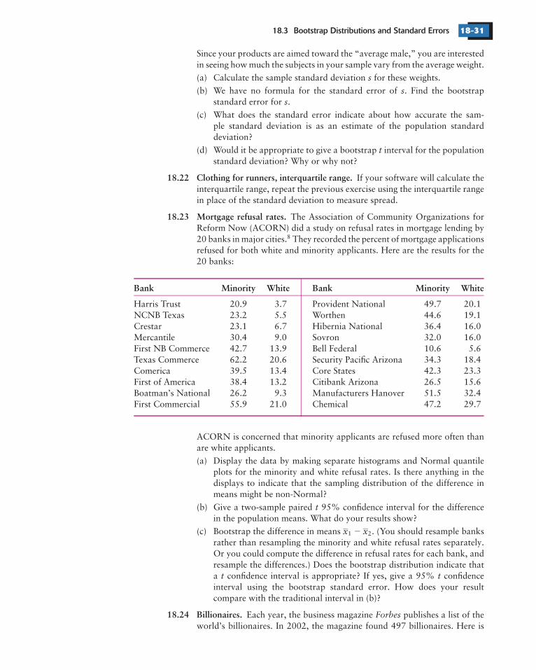
The Association of Community Organizations forReform Now (ACORN) did a study on refusal rates in mortgage lending by20 banks in major cities. They recorded the percent of mortgage applicationsrefused for both white and minority applicants. Here are the results for the20 banks:
Harris Trust 20.9 3.7 Provident National 49.7 20.1NCNB Texas 23.2 5.5 Worthen 44.6 19.1Crestar 23.1 6.7 Hibernia National 36.4 16.0Mercantile 30.4 9.0 Sovron 32.0 16.0First NB Commerce 42.7 13.9 Bell Federal 10.6 5.6Texas Commerce 62.2 20.6 Security Pacific Arizona 34.3 18.4Comerica 39.5 13.4 Core States 42.3 23.3First of America 38.4 13.2 Citibank Arizona 26.5 15.6Boatman’s National 26.2 9.3 Manufacturers Hanover 51.5 32.4First Commercial 55.9 21.0 Chemical 47.2 29.7
ACORN is concerned that minority applicants are refused more often thanare white applicants.
(a) Display the data by making separate histograms and Normal quantileplots for the minority and white refusal rates. Is there anything in thedisplays to indicate that the sampling distribution of the difference inmeans might be non-Normal?
(b) Give a two-sample paired 95% confidence interval for the differencein the population means. What do your results show?
(c) Bootstrap the difference in means . (You should resample banksrather than resampling the minority and white refusal rates separately.Or you could compute the difference in refusal rates for each bank, andresample the differences.) Does the bootstrap distribution indicate thata confidence interval is appropriate? If yes, give a 95% confidenceinterval using the bootstrap standard error. How does your resultcompare with the traditional interval in (b)?
Each year, the business magazine publishes a list of theworld’s billionaires. In 2002, the magazine found 497 billionaires. Here is
�
Bootstrap Methods and Permutation Tests18-32 CHAPTER 18 �
18.4 How Accurate Is a BootstrapDistribution?
SOURCES OF VARIATION IN A BOOTSTRAP DISTRIBUTION
�
18.25 Seeking the source of the skew.
�This section is optional.
9
1 2
The sampling distribution of a statistic displays the variation in the statisticdue to selecting samples at random from the population. We understandthat the statistic will vary from sample to sample, so that inference aboutthe population must take this random variation into account. For example,the margin of error in a confidence interval expresses the uncertainty dueto sampling variation. Now we have used the bootstrap distribution as asubstitute for the sampling distribution. We thus introduce another source ofrandom variation: resamples are chosen at random from the original sample.
Bootstrap distributions and conclusions based on them include twosources of random variation:
1. The original sample is chosen at random from the population.
2. Bootstrap resamples are chosen at random from the originalsample.
Figure 18.13 shows the entire process. The population distribution (topleft) has two peaks and is clearly not close to Normal. Below the figureare histograms of five random samples from this population, each of size50. The sample means are marked on each histogram. These vary fromsample to sample. The distribution of the -values from all possible samples
Forbes
x x
xx
the wealth, as estimated by and rounded to the nearest $100 million,of an SRS of 20 of these billionaires:
8.6 1.3 5.2 1.0 2.5 1.8 2.7 2.4 1.4 3.05.0 1.7 1.1 5.0 2.0 1.4 2.1 1.2 1.5 1.0
You are interested in (vaguely) “the wealth of typical billionaires.” Boot-strap an appropriate statistic, inspect the bootstrap distribution, and drawconclusions based on this sample.
Why is the bootstrap distributionof the difference in mean Verizon and CLEC repair times in Figure18.10 so skewed? Let’s investigate by bootstrapping the mean ofthe CLEC data and comparing it with the bootstrap distribution for themean for Verizon customers.
(a) Bootstrap the mean for the CLEC data. Compare the bootstrap distri-bution with the bootstrap distribution of the Verizon repair times inFigure 18.3.
(b) Given what you see in part (a), what is the source of the skew in thebootstrap distribution of the difference in means ?�
CA
SE1
8.1

–3 µ µ
µ
3 30 06
0 x
x
x x3 3 30 0
Sample 1
0 03 3 0 3x x
Sample 2
0 0 0x x x3 3 3
Sample 3
0 0 0x x x3 3 3
Sample 4
0 0 0x x x3 3 3
Sample 5
Population distribution Sampling distribution
Bootstrap distribution 6for
Sample 1
Bootstrap distributionfor
Sample 1
Bootstrap distributionforSample 2
Bootstrap distributionfor
Sample 3
Bootstrap distributionfor
Sample 4
Bootstrap distributionforSample 5
Bootstrap distribution 2for
Sample 1
Bootstrap distribution 3for
Sample 1
Bootstrap distribution 4for
Sample 1
Bootstrap distribution 5for
Sample 1
Population mean =Sample mean = x–
––
–
–
–
– – –
– –
– –
– –
–
FIGURE 18.13 Five random samples ( 50) from the same population, with a bootstrapdistribution for the sample mean formed by resampling from each of the five samples. At theright are five more bootstrap distributions from the first sample. In all cases, the mean of thebootstrap distribution is nearly indistinguishable from , so is not shown separately.
n
x
�
Bootstrap Methods and Permutation Tests18-34 CHAPTER 18 �
�
�
�
Bootstrapping small samples
�
� �
is the sampling distribution. This sampling distribution appears to the right ofthe population distribution. It is close to Normal, as we expect becauseof the central limit theorem.
Now draw 1000 resamples from an original sample, calculate foreach resample, and present the 1000 ’s in a histogram. This is a bootstrapdistribution for . The middle column in Figure 18.13 displays boot-strap distributions based on 1000 resamples from each of the five samples.The right column shows the results of repeating the resampling from thefirst sample five more times. Comparing the five bootstrap distributions inthe middle column shows the effect of the random choice of the originalsamples. Comparing the six bootstrap distributions drawn from the firstsample shows the effect of the random resampling. Here’s what we see:
Each bootstrap distribution is centered close to the value of from itsoriginal sample, whereas the sampling distribution is centered at thepopulation mean .
The shape and spread of the bootstrap distributions in the middle columnalso vary a bit. That is, shape and spread also depend on the originalsample, but the variation from sample to sample is not great. The shapeand spread of all of the bootstrap distributions resemble those of thesampling distribution.
The six bootstrap distributions from the same sample are very similar inshape, center, and spread. That is, random resampling adds little variationto the variation due to the random choice of the original sample from thepopulation.
Figure 18.13 reinforces facts that we have already relied on. If a bootstrapdistribution is based on a moderately large sample from the population, itsshape and spread don’t depend heavily on the original sample and do informus about the shape and spread of the sampling distribution. Bootstrapdistributions do not have the same center as the sampling distribution; theymimic bias, not the actual center. The figure also illustrates an importantnew fact: the bootstrap resampling process (using 1000 or more resamples)introduces little additional variation.
We now know that almost all of the variation among bootstrap distributionsfor a statistic such as the mean comes from the random selection ofthe original sample from the population. We also know that in generalstatisticians prefer large samples because small samples give more variableresults. This general fact is also true for bootstrap procedures.
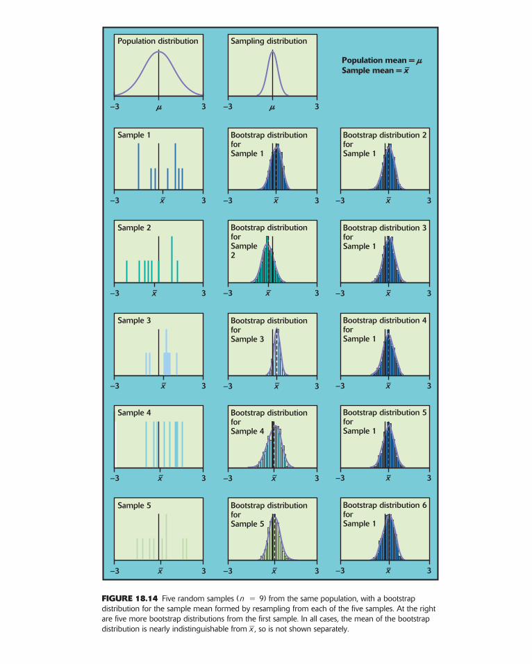
Figure 18.14 repeats Figure 18.13, with two important differences. Thefive original samples are only of size 9, rather than the 50 ofFigure 18.13. The population distribution (top left) is Normal, so that thesampling distribution of is Normal despite the small sample size. Thebootstrap distributions in the middle column show more variation in shapeand spread than those for larger samples in Figure 18.13. Notice, for exam-ple, how the skewness of the fourth sample produces a skewed bootstrap
xx
x
x
n n
x
–
– –
–3 � 3
Population distribution
–3 � 3
Sampling distribution
–3 3
Bootstrap distributionforSample 1
–3 x–
– – –
– – –
– – –
– – –
x –3 3
Bootstrap distribution 2forSample 1
x
–3 3
Bootstrap distribution 3forSample 1
x
–3 3
Bootstrap distribution 4forSample 1
x
–3 3
Bootstrap distribution 5forSample 1
x
–3 3
Bootstrap distribution 6forSample 1
x
–3 3
Bootstrap distributionforSample2
x
–3 3
Bootstrap distributionforSample 3
x
–3 3
Bootstrap distributionforSample 4
x
–3 3
Bootstrap distributionforSample 5
x
3
Sample 1
–3 x 3
Sample 2
–3 x 3
Sample 3
–3 x 3
Sample 4
–3 x 3
Sample 5
Population mean =Sample mean = x
�
FIGURE 18.14 Five random samples ( 9) from the same population, with a bootstrapdistribution for the sample mean formed by resampling from each of the five samples. At the rightare five more bootstrap distributions from the first sample. In all cases, the mean of the bootstrapdistribution is nearly indistinguishable from , so is not shown separately.
n
x
�
Bootstrap Methods and Permutation Tests18-36 CHAPTER 18 �
Bootstrapping a sample median
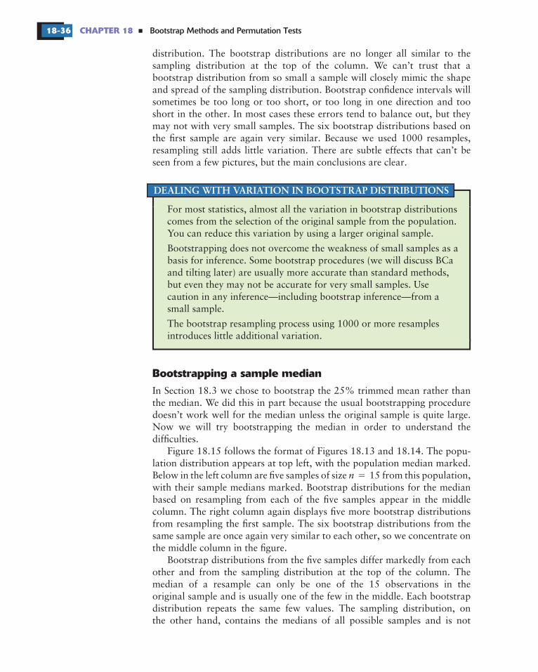
DEALING WITH VARIATION IN BOOTSTRAP DISTRIBUTIONS
�
distribution. The bootstrap distributions are no longer all similar to thesampling distribution at the top of the column. We can’t trust that abootstrap distribution from so small a sample will closely mimic the shapeand spread of the sampling distribution. Bootstrap confidence intervals willsometimes be too long or too short, or too long in one direction and tooshort in the other. In most cases these errors tend to balance out, but theymay not with very small samples. The six bootstrap distributions based onthe first sample are again very similar. Because we used 1000 resamples,resampling still adds little variation. There are subtle effects that can’t beseen from a few pictures, but the main conclusions are clear.
For most statistics, almost all the variation in bootstrap distributionscomes from the selection of the original sample from the population.You can reduce this variation by using a larger original sample.
Bootstrapping does not overcome the weakness of small samples as abasis for inference. Some bootstrap procedures (we will discuss BCaand tilting later) are usually more accurate than standard methods,but even they may not be accurate for very small samples. Usecaution in any inference—including bootstrap inference—from asmall sample.
The bootstrap resampling process using 1000 or more resamplesintroduces little additional variation.
In Section 18.3 we chose to bootstrap the 25% trimmed mean rather thanthe median. We did this in part because the usual bootstrapping proceduredoesn’t work well for the median unless the original sample is quite large.Now we will try bootstrapping the median in order to understand thedifficulties.
Figure 18.15 follows the format of Figures 18.13 and 18.14. The popu-lation distribution appears at top left, with the population median marked.Below in the left column are five samples of size 15 from this population,with their sample medians marked. Bootstrap distributions for the medianbased on resampling from each of the five samples appear in the middlecolumn. The right column again displays five more bootstrap distributionsfrom resampling the first sample. The six bootstrap distributions from thesame sample are once again very similar to each other, so we concentrate onthe middle column in the figure.
Bootstrap distributions from the five samples differ markedly from eachother and from the sampling distribution at the top of the column. Themedian of a resample can only be one of the 15 observations in theoriginal sample and is usually one of the few in the middle. Each bootstrapdistribution repeats the same few values. The sampling distribution, onthe other hand, contains the medians of all possible samples and is not
n

–4 M 10
Populationdistribution
–4 M 10
Samplingdistribution
–4 m 10
Bootstrapdistribution
forSample 1
–4 m 10
Bootstrapdistribution 2
forSample 1
–4 m 10
Bootstrapdistribution 3
forSample 1
–4 m 10
Bootstrapdistribution 4
forSample 1
–4 m 10
Bootstrapdistribution 5
forSample 1
–4 m 10
Bootstrapdistribution 6
forSample 1
–4 m 10
Bootstrapdistribution
forSample 2
–4 m 10
Bootstrapdistribution
forSample 3
–4 m 10
Bootstrapdistribution
forSample 4
–4 m 10
Bootstrapdistribution
forSample 5
–4 m 10
Sample 1
–4 m 10
Sample 2
–4 m 10
Sample 3
–4 m 10
Sample 4
–4 m 10
Sample 5
Population median = MSample median = m
FIGURE 18.15 Five random samples ( 15) from the same population, with a bootstrap distribu-tion for the sample median formed by resampling from each of the five samples. At the right are fivemore bootstrap distributions from the first sample.
n �
Bootstrap Methods and Permutation Tests18-38 CHAPTER 18
ECTION UMMARY
ECTION XERCISES
�
�
�
�
S
S
18.4 S
18.4 E18.26 The effect of sample size: Normal population.
18.27 The effect of sample size: non-Normal population.
�
�
� �
confined to a few values. The difficulty is somewhat less when is even,because the median is then the average of 2 observations. It is much less formoderately large samples, say, 100 or more. Bootstrap standard errorsand confidence intervals from such samples are reasonably accurate, thoughthe shapes of the bootstrap distributions may still appear odd. You can seethat the same difficulty will occur for small samples with other statistics,such as the quartiles, that are calculated from just 1 or 2 observations froma sample.
There are more advanced variations of the bootstrap idea that improveperformance for small samples and for statistics such as the median andquartiles. In particular, your software may offer the “smoothed bootstrap”for use with medians and quartiles. Unless you have expert advice orundertake further study, avoid bootstrapping the median and quartilesunless your sample is rather large.
Almost all of the variation in a bootstrap distribution is due to theselection of the original random sample from the population. Theresampling process introduces little additional variation.
Bootstrap distributions based on small samples can be quite variable.Their shape and spread reflect the characteristics of the sample and maynot accurately estimate the shape and spread of the sampling distribution.
Bootstrapping is unreliable for statistics like the median and quartileswhen the sample size is small. The bootstrap distributions tend to bebroken up (discrete) and highly variable in shape.
N . , .
xn
nx
n n
n
n
Your statistical software nodoubt includes a function to generate samples from Normal distributions.Set the mean to 8.4 and the standard deviation to 14.7. You can think ofall the numbers produced by this function if it ran forever as a populationthat has very close to the (8 4 14 7) distribution. Samples produced by thefunction are samples from this population.(a) What is the exact sampling distribution of the sample mean for a
sample of size from this population?(b) Draw an SRS of size 10 from this population. Bootstrap the sample
mean using 1000 resamples from your sample. Give a histogram andNormal quantile plot of the bootstrap distribution and the bootstrapstandard error.
(c) Repeat the same process for samples of sizes 40 and 160.(d) Write a careful description comparing the three bootstrap distributions
and also comparing them with the exact sampling distribution. Whatare the effects of increasing the sample size?
The datafor Example 18.7 include 1664 repair times for customers ofVerizon, the local telephone company in their area. In thatexample these observations formed a sample. Now we will treat these
CA
SE1
8.1
18.5 Bootstrap Confidence Intervals 18-39
18.5 Bootstrap Confidence Intervals
Bootstrap percentiles as a check
18.28 Normal versus non-Normal populations.
�
�
�
� �
To this point, we have met just one type of inference procedure based onresampling: bootstrap confidence intervals. We can calculate a bootstrapconfidence interval for any parameter by bootstrapping the correspondingstatistic (the plug-in principle). We don’t need conditions on the populationor special knowledge about the sampling distribution of the statistic. Theflexible and almost automatic nature of bootstrap intervals is wonderful—but there is a catch. These intervals work well only when the bootstrapdistribution tells us that the sampling distribution is approximately Normaland has small bias. How can we know whether these conditions are met wellenough to trust the confidence interval? And what can we do if we don’t trustthe bootstrap interval? This section deals with these important questions.We’ll learn a quick way to check confidence intervals for accuracy andlearn alternative ways to calculate confidence intervals when intervalsaren’t accurate.
Confidence intervals are based on the sampling distribution of a statistic.A 95% confidence interval starts by marking off the central 95% of thesampling distribution. The critical values in any confidence interval area shortcut to marking off this central 95%. The shortcut requires specialconditions that are not always met, so intervals are not always appropriate.One way to check whether intervals (using either bootstrap or formula
..
x n
nx
n n
x
x
t t
t
tt
t
t t
tt
1664 observations as a population. The population distribution appears inFigure 18.9. The population mean is 8 4, and the population standarddeviation is 14 7.
(a) Although we don’t know the shape of the sampling distribution of thesample mean for a sample of size from this population, we do knowthe mean and standard deviation of this distribution. What are they?
(b) Draw an SRS of size 10 from this population. Bootstrap the samplemean using 1000 resamples from your sample. Give a histogram andNormal quantile plot of the bootstrap distribution and the bootstrapstandard error.
(c) Repeat the same process for samples of sizes 40 and 160.
(d) Write a careful description comparing the three bootstrap distributions.What are the effects of increasing the sample size?
The populations in thetwo previous exercises have the same mean and standard deviation,but one is very close to Normal and the other is strongly non-Normal. Based on your work in these exercises, how does non-Normality ofthe population affect the bootstrap distribution of ? How does it affect thebootstrap standard error? Do either of these effects diminish when we startwith a larger sample? Explain what you have observed based on what youknow about the sampling distribution of and the way in which bootstrapdistributions mimic the sampling distribution.
�
�
CA
SE1
8.1
Bootstrap Methods and Permutation Tests18-40 CHAPTER 18
Seattle real estate sales: the trimmed meanEXAMPLE 18.9
�
APPLY YOURKNOWLEDGE
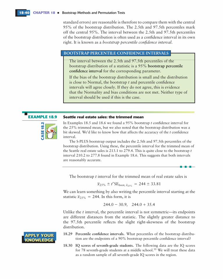
BOOTSTRAP PERCENTILE CONFIDENCE INTERVALS
bootstrap percentileconfidence interval
18.29 Percentile confidence intervals.
18.30 IQ scores of seventh-grade students.
� �
�
, x� �
�
�
25% boot
25%
10
standard errors) are reasonable is therefore to compare them with the central95% of the bootstrap distribution. The 2.5th and 97.5th percentiles markoff the central 95%. The interval between the 2.5th and 97.5th percentilesof the bootstrap distribution is often used as a confidence interval in its ownright. It is known as a .
The interval between the 2.5th and 97.5th percentiles of thebootstrap distribution of a statistic is a 95%
for the corresponding parameter.
If the bias of the bootstrap distribution is small and the distributionis close to Normal, the bootstrap and percentile confidenceintervals will agree closely. If they do not agree, this is evidencethat the Normality and bias conditions are not met. Neither type ofinterval should be used if this is the case.
The bootstrap interval for the trimmed mean of real estate sales is
SE 244 33 81
We can learn something by also writing the percentile interval starting at thestatistic 244. In this form, it is
244 0 30 9 244 0 35 4
Unlike the interval, the percentile interval is not symmetric—its endpointsare different distances from the statistic. The slightly greater distance tothe 97.5th percentile reflects the slight right-skewness of the bootstrapdistribution.
25%
t
t
t
bootstrap percentile confidence interval
t
t
x t .
x
. . , . .
t
In Examples 18.5 and 18.6 we found a 95% bootstrap confidence interval forthe 25% trimmed mean, but we also noted that the bootstrap distribution was abit skewed. We’d like to know how that affects the accuracy of the confidenceinterval.
The S-PLUS bootstrap output includes the 2.5th and 97.5th percentiles of thebootstrap distribution. Using these, the percentile interval for the trimmed mean ofthe Seattle real estate sales is 213.1 to 279.4. This is quite close to the bootstrapinterval 210.2 to 277.8 found in Example 18.6. This suggests that both intervalsare reasonably accurate.
What percentiles of the bootstrap distribu-tion are the endpoints of a 90% bootstrap percentile confidence interval?
The following data are the IQ scoresfor 78 seventh-grade students at a middle school. We will treat these dataas a random sample of all seventh-grade IQ scores in the region.
APPLY YOURKNOWLEDGE
CA
SE18
.2
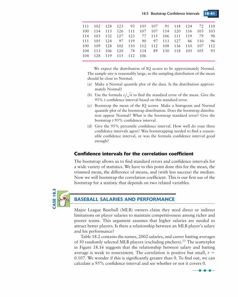
18.5 Bootstrap Confidence Intervals 18-41
Confidence intervals for the correlation coefficient
BASEBALL SALARIES AND PERFORMANCE
�
11
��
The bootstrap allows us to find standard errors and confidence intervals fora wide variety of statistics. We have to this point done this for the mean, thetrimmed mean, the difference of means, and (with less success) the median.Now we will bootstrap the correlation coefficient. This is our first use of thebootstrap for a statistic that depends on two related variables.
Major League Baseball (MLB) owners claim they need direct or indirectlimitations on player salaries to maintain competitiveness among richer andpoorer teams. This argument assumes that higher salaries are needed toattract better players. Is there a relationship between an MLB player’s salaryand his performance?
Table 18.2 contains the names, 2002 salaries, and career batting averagesof 50 randomly selected MLB players (excluding pitchers). The scatterplotin Figure 18.16 suggests that the relationship between salary and battingaverage is weak to nonexistent. The correlation is positive but small,0 107. We wonder if this is significantly greater than 0. To find out, we cancalculate a 95% confidence interval and see whether or not it covers 0.
s nt
t
r.
111 102 128 123 93 105 107 91 118 124 72 110100 114 113 126 111 107 107 114 120 116 103 103114 103 132 127 123 77 115 106 111 119 79 98111 105 124 97 119 90 97 113 127 86 110 96100 109 128 102 110 112 112 108 136 110 107 112104 113 106 120 74 114 89 130 118 103 105 93104 128 119 115 112 106
We expect the distribution of IQ scores to be approximately Normal.The sample size is reasonably large, so the sampling distribution of the meanshould be close to Normal.
(a) Make a Normal quantile plot of the data. Is the distribution approxi-mately Normal?
(b) Use the formula to find the standard error of the mean. Give the95% confidence interval based on this standard error.
(c) Bootstrap the mean of the IQ scores. Make a histogram and Normalquantile plot of the bootstrap distribution. Does the bootstrap distribu-tion appear Normal? What is the bootstrap standard error? Give thebootstrap 95% confidence interval.
(d) Give the 95% percentile confidence interval. How well do your threeconfidence intervals agree? Was bootstrapping needed to find a reason-able confidence interval, or was the formula confidence interval goodenough?
CA
SE18.3
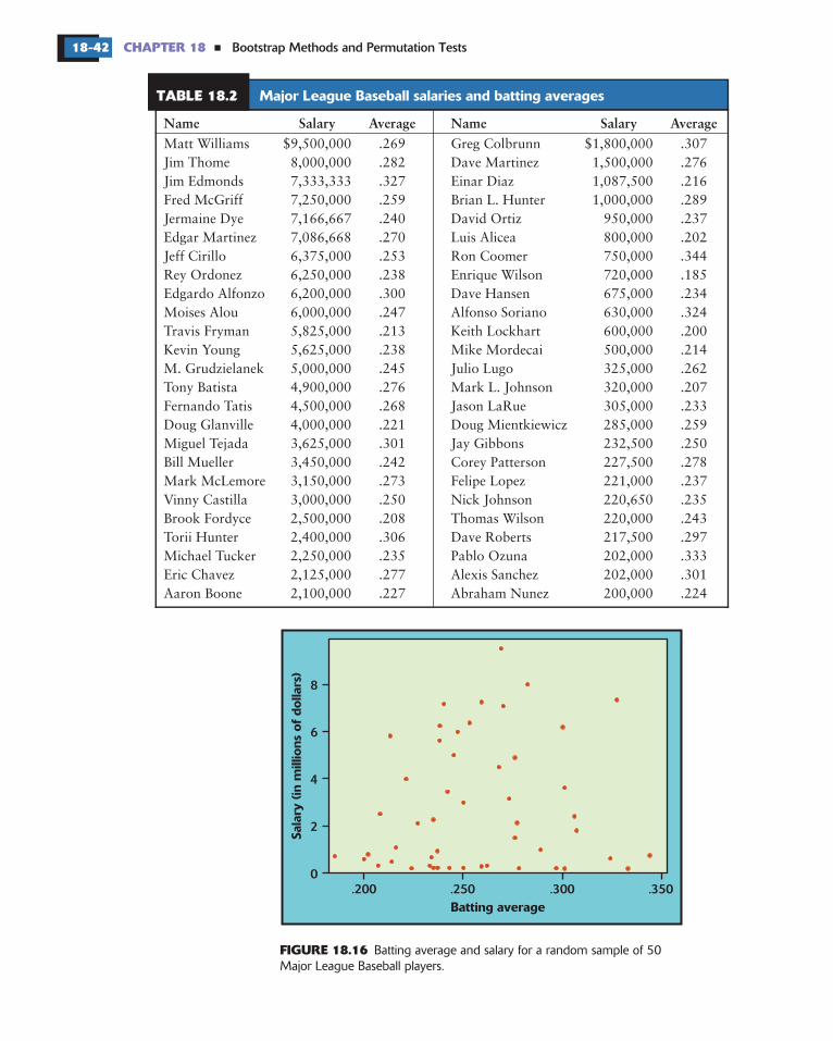
0
2
4
6
8
.200 .250 .300 .350Batting average
Sala
ry (
in m
illio
ns o
f do
llars
)
Bootstrap Methods and Permutation Tests18-42 CHAPTER 18
FIGURE 18.16
�
Batting average and salary for a random sample of 50Major League Baseball players.
Name Salary Average Name Salary AverageMatt Williams $9,500,000 .269 Greg Colbrunn $1,800,000 .307Jim Thome 8,000,000 .282 Dave Martinez 1,500,000 .276Jim Edmonds 7,333,333 .327 Einar Diaz 1,087,500 .216Fred McGriff 7,250,000 .259 Brian L. Hunter 1,000,000 .289Jermaine Dye 7,166,667 .240 David Ortiz 950,000 .237Edgar Martinez 7,086,668 .270 Luis Alicea 800,000 .202Jeff Cirillo 6,375,000 .253 Ron Coomer 750,000 .344Rey Ordonez 6,250,000 .238 Enrique Wilson 720,000 .185Edgardo Alfonzo 6,200,000 .300 Dave Hansen 675,000 .234Moises Alou 6,000,000 .247 Alfonso Soriano 630,000 .324Travis Fryman 5,825,000 .213 Keith Lockhart 600,000 .200Kevin Young 5,625,000 .238 Mike Mordecai 500,000 .214M. Grudzielanek 5,000,000 .245 Julio Lugo 325,000 .262Tony Batista 4,900,000 .276 Mark L. Johnson 320,000 .207Fernando Tatis 4,500,000 .268 Jason LaRue 305,000 .233Doug Glanville 4,000,000 .221 Doug Mientkiewicz 285,000 .259Miguel Tejada 3,625,000 .301 Jay Gibbons 232,500 .250Bill Mueller 3,450,000 .242 Corey Patterson 227,500 .278Mark McLemore 3,150,000 .273 Felipe Lopez 221,000 .237Vinny Castilla 3,000,000 .250 Nick Johnson 220,650 .235Brook Fordyce 2,500,000 .208 Thomas Wilson 220,000 .243Torii Hunter 2,400,000 .306 Dave Roberts 217,500 .297Michael Tucker 2,250,000 .235 Pablo Ozuna 202,000 .333Eric Chavez 2,125,000 .277 Alexis Sanchez 202,000 .301Aaron Boone 2,100,000 .227 Abraham Nunez 200,000 .224
TABLE 18.2 Major League Baseball salaries and batting averages

–0.2 0.0 0.2 0.4Correlation coefficient
(a)
–0.2
0.0
0.2
0.4
–2 0 2z-score
Cor
rela
tion
coe
ffic
ient
(b)
ObservedMean
18.5 Bootstrap Confidence Intervals 18-43
FIGURE 18.17
Bootstrapping the correlationEXAMPLE18.10
The bootstrap distribution and Normal quantileplot for the correlation for 1000 resamples from the baseballplayer data in Table 18.2. The solid double-ended arrow below thedistribution is the interval, and the dashed arrow is the percentileinterval.
r
t
t
We use the same bootstrap procedures to find a confidence interval for thecorrelation coefficient as for other statistics. There is one point to note: becauseeach observation consists of the batting average and salary for one player, weresample players (that is, observations). Resampling batting averages and salariesseparately would lose the tie between a player’s batting average and his salary.
Figure 18.17 shows the bootstrap distribution and Normal quantile plot forthe sample correlation for 1000 resamples from the 50 players in our sample.The bootstrap distribution is reasonably Normal and has small bias, so a 95%bootstrap confidence interval appears reasonable.
CA
SE18
.3
Bootstrap Methods and Permutation Tests18-44 CHAPTER 18 �
More accurate bootstrap confidence intervals
APPLY YOURKNOWLEDGE
accurate
, r
, r
18.31 Percentiles as an aid in detecting non-Normality.
18.32 Wages and length of service.
�
accurate
�
�
�
�
� �
�
boot
boot
The confidence intervals give a wide range for the population correlation,and both include zero. These data do not provide significant evidence thatthere is a relationship between salary and batting average. There may bea relationship that could be found with a larger data set, but the evidencefrom this data set suggests that any relationship is fairly weak. Of course,batting average is only one facet of a player’s performance. It is possiblethat we would discover a significant salary-performance relationship if weincluded several measures of performance.
No method for obtaining confidence intervals produces exactly the intendedconfidence level in practice. When we compute what is supposed to be a95% confidence interval, our method may give intervals that in fact capturethe true parameter value less often, say, 92% or 85% of the time. Or insteadof missing 2.5% of the time on each side, the method may in some settingsmiss 1% of the time on one side and 4% of the time on the other, giving abiased picture of where the parameter is.
We say that a method for obtaining 95% confidence intervals isin a particular setting if 95% of the time it produces intervals that capturethe parameter and if the 5% misses are shared equally between high andlow misses. Confidence intervals are never exactly accurate because the
. t
r t . . .
. .
. , .
. , . . . , . .
. , .
t
t
The bootstrap standard error is SE 0 125. The interval using thebootstrap standard error is
SE 0 107 (2 01)(0 125)
0 107 0 251
( 0 144 0 358)
The bootstrap percentile interval is
(2 5th percentile 97 5th percentile) (0 107 0 235 0 107 0 249)
( 0 128 0 356)
The two confidence intervals are in reasonable agreement.
It is difficult tosee any significant asymmetry in the bootstrap distribution of thecorrelation of Example 18.10. Compare the percentiles and theinterval; does the difference between these suggest any skewness?
Table 10.1 (page 587) reports thewages and length of service for a random sample of 59 womenwho hold customer service jobs in Indiana banks. In Example 10.4,using a test that assumes a jointly Normal distribution for these variables,we found a highly significant relationship between wages and length ofservice. We may prefer inference that is not based on a Normal model.Bootstrap the correlation for these data. Give the bootstrap and bootstrappercentile confidence intervals for the population correlation. Are theseintervals trustworthy here? What do you conclude about the population?
� �
�
�
�
�
CA
SE1
0.1
APPLY YOURKNOWLEDGE
CA
SE1
8.3
18.5 Bootstrap Confidence Intervals 18-45
Seattle real estate sales: the meanEXAMPLE18.11
�
�
�
Bootstrap tilting and BCa intervals
bootstrap bias-corrected accelerated (BCa) bootstrap tiltingBCabootstrap tilting
conditions under which they work are never exactly satisfied in practice.The traditional intervals, although reasonably robust, are affected by lackof Normality in the sampling distribution of the sample mean, especiallyskewness. Although the central limit theorem tells us that the samplingdistribution of the mean becomes nearly Normal as the size of the sampleincreases, the effect of a skewed population can persist in the samplingdistribution even for quite large samples.
One advantage of the bootstrap is that it allows us to check for skewnessin a sampling distribution by inspecting the bootstrap distribution. We canalso compare the bootstrap and bootstrap percentile confidence intervals.When the sampling distribution is skewed, the percentile interval is shiftedin the direction of the skewness, relative to the interval. The intervals inboth Example 18.9 and Example 18.10 reveal some right-skewness, thoughnot enough to invalidate inference. The and percentile intervals may notbe sufficiently accurate when
the statistic is strongly biased, as indicated by the bias estimate from thebootstrap,
the sampling distribution of the statistic is clearly skewed, as indicated bythe bootstrap distribution and by comparing the and percentile intervals,or
high accuracy is needed because the stakes are high (large sums of moneyor public welfare).
Most confidence interval procedures are more accurate for larger samplesizes. The problem with and percentile procedures is that they improveonly slowly—they require 100 times more data to improve accuracy by afactor of 10—and so tend not to be very accurate except for quite largesample sizes. There are several bootstrap procedures that improve faster,requiring only 10 times more data to improve accuracy by a factor of 10.These procedures are quite accurate unless the sample size is very small. The
and methodsare accurate in a wide variety of settings, have reasonable computationrequirements (by modern standards), and do not produce excessively wideintervals.
These procedures are not as intuitively clear as the and percentilemethods, which is why we did not meet them earlier. Now that youunderstand the bootstrap, however, you should always use one of thesemore accurate methods if your software offers them.
t
t
t
t
t
t
t
The 2002 Seattle real estate sales data are strongly skewed (Figure 18.6), and theskewness persists in the sampling distribution of the mean (Figure 18.7). Generally,we prefer resistant measures of center such as the trimmed mean or median forskewed data. However, the mean is easily understood by the public and is neededfor some purposes, such as projecting taxes based on total sales value.
CA
SE18
.2

Number of Replications: 1000
Summary Statistics:Observed Mean Bias SE
mean 329.3 326.9 –2.383 43.9
Percentiles:2.5% 5.0% 95.0% 97.5%
mean 252.5 261.7 408.3 433.1
BCa Confidence Limits:2.5% 5% 95% 97.5%
mean 270 279.6 442.7 455.7
Tilting Confidence Limits (maximum-likelihood tilting):2.5% 5% 95% 97.5%
mean 265 274.4 434.2 458.7
Bootstrap Methods and Permutation Tests18-46 CHAPTER 18
FIGURE 18.18
�
S-PLUS output for bootstrapping the meanof the Seattle real estate sales price data. From this outputyou can obtain the bootstrap and percentile intervals, whichare not accurate for these data. You can also obtain the BCaand tilting intervals, the recommended methods.
t
APPLY YOURKNOWLEDGE
18.33 Comparing intervals.
� ��
� �
� �
t
. . , . . . , .
. . , . . . , .
t t
t
t x t s n
x
The bootstrap and percentile intervals aren’t reliable when the samplingdistribution of the statistic is skewed. Figure 18.18 shows software output thatallows us to obtain more accurate confidence intervals. The BCa interval is
(329 3 59 2 329 3 126 4) (270 0 455 7)
and the tilting interval is
(329 3 64 3 329 3 129 5) (265 0 458 7)
The intervals agree closely (we usually find only small differences between highlyaccurate procedures). Both are strongly asymmetrical—the upper endpoint is abouttwice as far from the sample mean as the lower endpoint—reflecting the strongright-skewness of the data.
In this example, both endpoints of the less-accurate procedures— , bootstrap ,and percentile intervals—are too low. These intervals are too likely (greater than2.5%) to fall below the population mean and are not likely enough to fall abovethe population mean. They give a biased picture of where the true mean is likelyto be. If you use these intervals to budget how much you would need to be 95%confident of affording an average home, your estimate would be too low.
Use the software output in Figure 18.18 togive the bootstrap and percentile 95% confidence intervals forthe mean of all 2002 real estate sales in Seattle. Also give thetraditional one-sample interval, . Example 18.11 reports theBCa and tilting intervals. Make a picture that compares all five confidenceintervals by drawing a vertical line at and placing the intervals one
�
�
�
� CA
SE1
8.2
APPLY YOURKNOWLEDGE
18.5 Bootstrap Confidence Intervals 18-47
How the BCa and tilting intervals work
18.34 Comparing intervals.
18.35 Wages and length of service.
25%
The BCa confidence interval endpoints are percentiles of the bootstrapdistribution that are adjusted to correct for bias and skewness in thedistribution. For example, the endpoints of the BCa 95% confidence intervalfor the mean of the 2002 Seattle real estate data are the 4.3th and 98.8thpercentiles of the bootstrap distribution, rather than 2.5th and 97.5thpercentiles. If the statistic is biased upward (that is, if it tends to be too large),the BCa bias correction moves the endpoints to the left. If the bootstrapdistribution is skewed to the right, the BCa incorporates a correction tomove the endpoints even farther to the right; this may seem counterintuitive,but it is the correct action. Details of the computations are a bit advanced,so we rely on software to calculate these intervals.
The tilting interval, in contrast, works by adjusting the process ofrandomly forming resamples. To calculate the left endpoint of the interval,it starts by finding a pseudopopulation that is similar to the sample exceptthat the bootstrap distribution from this population has its 97.5th percentileequal to the observed statistic from our SRS. Then the left endpoint of thetilting interval is the parameter of that pseudo-population. Similarly, theright endpoint of the interval is the parameter of a pseudo-population whosebootstrap distribution has its 2.5th percentile equal to the observed statisticof the SRS. We again rely on software to handle the calculations.
Bootstrap tilting is more efficient than other bootstrap intervals, requiringonly about 1/37 as many resamples as BCa intervals for similarly accurateresults. If we require high accuracy, 1000 resamples is often not enough forthe BCa interval; 5000 resamples would be better.
t
t
tx
t
tt
above the other on this line. Describe how the intervals compare. In practicalterms, what kind of errors would you make by using a interval or percentileinterval instead of a tilting or BCa interval?
The bootstrap distribution of the 25%trimmed mean for the Seattle real estate sales (Figure 18.8) isnot strongly skewed. We were willing in Example 18.6 to give the95% bootstrap confidence interval for the trimmed mean of the population.Was that wise? Bootstrap the trimmed mean and give all of the bootstrap95% confidence intervals: , percentile, BCa, and tilting. Make a picturethat compares these intervals by drawing a vertical line at and placingthe intervals one above the other on this line. Describe how the intervalscompare. Is the interval reasonably accurate?
Table 10.1 (page 587) reports thewages and length of service for a random sample of 59 women whohold customer service jobs in Indiana banks. Exercise 18.32 askedyou to give a bootstrap confidence interval for the population correlationbetween these variables. In practice, you would use the BCa or tilting method.Bootstrap the correlation from the sample in Table 10.1 and compare theBCa and tilting intervals with the bootstrap and percentile intervals. Ifyou did Exercise 18.32, explain why the and percentile intervals you nowobtain differ slightly from those you found in the earlier exercise.
CA
SE1
8.2
CA
SE1
0.1

Bootstrap Methods and Permutation Tests18-48 CHAPTER 18
ECTION UMMARY
ECTION XERCISES
�
�
�
�
S
S
18.5 S
18.5 E
bootstrap percentile confidence interval
bootstrap tilting BCa
18.36 CLEC repair times.
While the BCa and tilting calculations are radically different, the resultstend to be about the same, except for random variation in the BCa if thenumber of resamples is less than about 5000. Both procedures are accurate,so we expect them to produce about the same results. Even BCa and tiltingconfidence intervals should be used cautiously when sample sizes are small,because there won’t be enough data to accurately determine the necessarycorrections for bias and skewness.
Both bootstrap and (when they exist) traditional and confidenceintervals require statistics with small bias and sampling distributions closeto Normal. We can check these conditions by examining the bootstrapdistribution for bias and lack of Normality.
The for 95% confidence is theinterval from the 2.5th percentile to the 97.5th percentile of the bootstrapdistribution. Agreement between the bootstrap and percentile intervals isan added check on the conditions needed by the interval. Do not use orpercentile intervals if these conditions are not met.
When bias or skewness is present in the bootstrap distribution, useeither a or interval. The and percentile intervals areinaccurate under these circumstances unless the sample sizes are very large.The tilting and BCa confidence intervals adjust for bias and skewness andare generally accurate except for small samples.
t
t
t z t
tt t
t
The CLEC data of Example 18.7 are stronglyskewed to the right. The 23 CLEC repair times (in hours) are
26.62 8.60 0 21.15 8.33 20.28 96.32 17.973.42 0.07 24.38 19.88 14.33 5.45 5.40 2.680 24.20 22.13 18.57 20.00 14.13 5.80
(a) Make a histogram and Normal quantile plot of the sample data, andfind the sample mean.
(b) Bootstrap the mean of the data. Plot the bootstrap distribution. Is itNormal? Do you expect any of the confidence intervals to be inaccurate?Why or why not?
(c) Find the bootstrap standard error and use it to create a 95% confidenceinterval.
(d) Find the 95% percentile, BCa, and tilting intervals.
(e) How do the intervals compare? Briefly explain the reasons for anydifferences.
(f) Suppose you were using these data and confidence intervals to determinestaffing levels for the coming year that you are confident would matchthe demand. What kind of errors would you make by using a intervalor percentile interval instead of a tilting or BCa interval?
CA
SE1
8.1

18.5 Bootstrap Confidence Intervals 18-49
18.37 Mean difference in repair times.
18.38 Really Normal data.
18.39 Clothing for runners.
18.40 Earnings of black male bank workers.
18.41 Bootstrap to check traditional inference.
��
t
t
N ,
t
ts n
t
In Example 18.7 we lookedat the mean difference between repair times for Verizon (ILEC)customers and customers of competing carriers (CLECs). Thebootstrap distribution was non-Normal with strong right-skewness, makinga confidence interval inappropriate.(a) Bootstrap the difference in means for the repair time data.(b) Find the BCa and bootstrap tilting 95% confidence intervals. Do they
agree closely? What do you conclude about mean repair times for allcustomers?
(c) In practical terms, what kind of errors would you make by using ainterval or percentile interval instead of a tilting or BCa interval?
In Exercise 18.19 you bootstrapped the mean of asimulated SRS from the standard Normal distribution (0 1) and foundthe standard error for the mean.(a) Create the 95% bootstrap percentile confidence interval for the mean
of the population. We know that the population mean is in fact 0. Doesthe confidence interval capture this mean?
(b) Compare the bootstrap percentile and bootstrap intervals. Do theseagree closely enough to indicate that these intervals are accurate?
In Exercise 18.21 you found the bootstrap standarderror of the standard deviation of the weights of male runners. Your companyis also interested in the average weight of its customers.(a) Give the 95% confidence interval for the mean weight of runners using
the standard error computed by formula.(b) Are there any data points that might strongly influence this confidence
interval?(c) Give a 95% bootstrap percentile confidence interval for the mean.
Compare your interval with your work in (a).(d) What conclusions can you draw about the population?
Table 1.8 (page 31) givesthe earnings for a random sample of black male hourly workersat National Bank.(a) Make a histogram and Normal quantile plot of the data. Choose a
statistic to measure the center of the distribution. Justify your choice interms of the shape of the distribution and the size of the sample.
(b) Bootstrap your statistic and report its standard error.(c) Choose a confidence interval based on the shape and bias of the
bootstrap distribution, and calculate it. What do you conclude aboutthe typical salary of black male hourly workers at National Bank?
Bootstrapping is a good way tocheck whether traditional inference methods are accurate for a given sample.Consider the following data:
109 123 118 99 121 134 126 114 129 123 171 124 111 125 128154 121 123 118 106 108 112 103 125 137 121 102 135 109 115125 132 134 126 116 105 133 111 112 118 117 105 107
(a) Examine the data graphically. Do they appear to violate any of theconditions needed to use the one-sample confidence interval for thepopulation mean?
CA
SE1
.2C
ASE
18
.1
Bootstrap Methods and Permutation Tests18-50 CHAPTER 18 �
18.42 More on checking traditional inference.
18.43 Iowa housing prices.
18.44 Iowa housing prices.
18.45 Weight as a predictor of car mileage.
18.46 Baseball salaries.
12
t
t
tt
t
t
t
(b) Calculate the 95% one-sample confidence interval for this sample.
(c) Bootstrap the mean, and inspect the bootstrap distribution. Does itsuggest that a interval should be reasonably accurate?
(d) Find the 95% bootstrap percentile interval. Does it agree with the one-sample interval? What do you conclude about the accuracy of theone-sample interval here?
Continue to work with the datagiven in the previous exercise.
(a) Find the bootstrap BCa or tilting 95% confidence interval. We believethat either interval is quite accurate.
(b) Does your opinion of the robustness of the confidence interval changewhen you compare it with the BCa or tilting interval?
(c) To check the accuracy of the one-sample confidence interval,would you generally use the bootstrap percentile or BCa (or tilting)interval?
Table 2.13 (page 165) gives the selling price, squarefootage, and age for a sample of 50 houses sold in Ames, Iowa.
(a) Make a histogram and Normal quantile plot of the prices. Based onthese plots, decide which statistic—mean, trimmed mean, or median—would be the most useful measure of the price of typical houses sold inAmes.
(b) Bootstrap that statistic and find its standard error.
(c) Plot the bootstrap distribution and describe its shape and bias. Choosean appropriate 95% confidence interval for this sampling distribution,and calculate it. Why did you choose this type of interval?
(d) What conclusion do you draw about Ames houses?
Bootstrap the correlation between selling price andsquare footage in the Ames, Iowa, housing data from Table 2.13 (page 165).Describe the bootstrap distribution, and give a 95% confidence interval thatis appropriate for these data. Explain your choice of interval. State yourconclusions from your analysis.
Table 18.3 gives weight in pounds andgas mileage in miles per gallon for a sample of cars from the 1990 modelyear.
(a) Make a scatterplot of the data. Characterize the relationship. Calculatethe sample correlation between weight and mileage.
(b) Bootstrap the correlation. Report an accurate confidence interval for thecorrelation and tell what it means.
(c) Calculate the least-squares regression line to predict mileage fromweight. What is the traditional confidence interval (page 596) forthe slope of the population regression line?
(d) Bootstrap the regression model. Give a 95% percentile confidenceinterval for the regression slope using the bootstrap.
Table 18.2 gives data on a sample of 50 baseballplayers.
(a) Find the least-squares regression line for predicting battingaverage from salary.
CA
SE18
.3
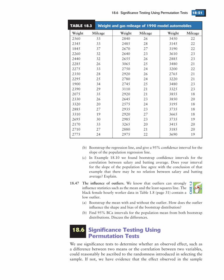
18.6 Significance Testing Using Permutation Tests 18-51
18.6 Significance Testing UsingPermutation Tests
Weight Mileage Weight Mileage Weight Mileage
18.47 The influence of outliers.
We use significance tests to determine whether an observed effect, such asa difference between two means or the correlation between two variables,could reasonably be ascribed to the randomness introduced in selecting thesample. If not, we have evidence that the effect observed in the sample
2560 33 2840 26 3450 222345 33 2485 28 3145 221845 37 2670 27 3190 222260 32 2640 23 3610 232440 32 2655 26 2885 232285 26 3065 25 3480 212275 33 2750 24 3200 222350 28 2920 26 2765 212295 25 2780 24 3220 211900 34 2745 25 3480 232390 29 3110 21 3325 232075 35 2920 21 3855 182330 26 2645 23 3850 203320 20 2575 24 3195 182885 27 2935 23 3735 183310 19 2920 27 3665 182695 30 2985 23 3735 192170 33 3265 20 3415 202710 27 2880 21 3185 202775 24 2975 22 3690 19
(b) Bootstrap the regression line, and give a 95% confidence interval for theslope of the population regression line.
(c) In Example 18.10 we found bootstrap confidence intervals for thecorrelation between salary and batting average. Does your intervalfor the slope of the population line agree with the conclusion of thatexample that there may be no relation between salary and battingaverage? Explain.
We know that outliers can stronglyinfluence statistics such as the mean and the least-squares line. Theblack female hourly worker data in Table 1.8 (page 31) contain alow outlier.
(a) Bootstrap the mean with and without the outlier. How does the outlierinfluence the shape and bias of the bootstrap distribution?
(b) Find 95% BCa intervals for the population mean from both bootstrapdistributions. Discuss the differences.
CA
SE1
.2
TABLE 18.3 Weight and gas mileage of 1990 model automobiles
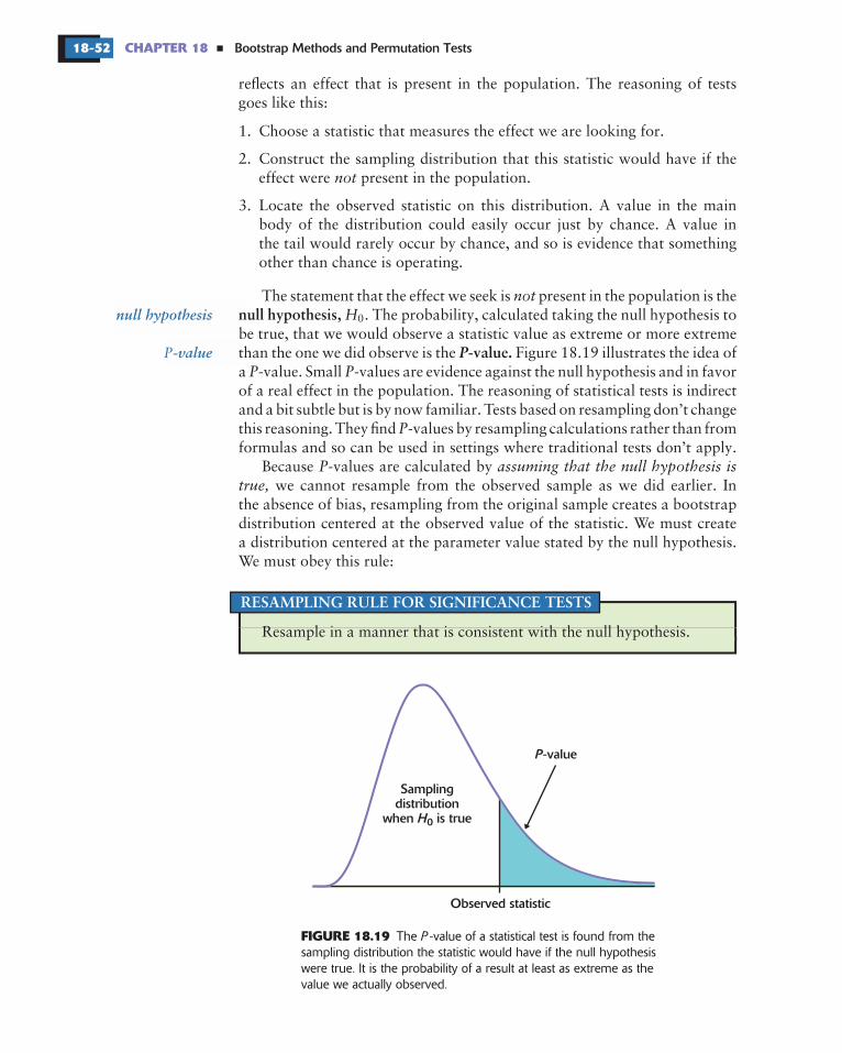
Samplingdistribution
when H0 is true
P-value
Observed statistic
Bootstrap Methods and Permutation Tests18-52 CHAPTER 18
FIGURE 18.19
�
The -value of a statistical test is found from thesampling distribution the statistic would have if the null hypothesiswere true. It is the probability of a result at least as extreme as thevalue we actually observed.
P
null hypothesis,
-value.
RESAMPLING RULE FOR SIGNIFICANCE TESTS
P
null hypothesis
-value
0
reflects an effect that is present in the population. The reasoning of testsgoes like this:
1. Choose a statistic that measures the effect we are looking for.
2. Construct the sampling distribution that this statistic would have if theeffect were present in the population.
3. Locate the observed statistic on this distribution. A value in the mainbody of the distribution could easily occur just by chance. A value inthe tail would rarely occur by chance, and so is evidence that somethingother than chance is operating.
The statement that the effect we seek is present in the population is the. The probability, calculated taking the null hypothesis to
be true, that we would observe a statistic value as extreme or more extremethan the one we did observe is the Figure 18.19 illustrates the idea ofa -value. Small -values are evidence against the null hypothesis and in favorof a real effect in the population. The reasoning of statistical tests is indirectand a bit subtle but is by now familiar. Tests based on resampling don’t changethis reasoning. They find -values by resampling calculations rather than fromformulas and so can be used in settings where traditional tests don’t apply.
Because -values are calculated bywe cannot resample from the observed sample as we did earlier. In
the absence of bias, resampling from the original sample creates a bootstrapdistribution centered at the observed value of the statistic. We must createa distribution centered at the parameter value stated by the null hypothesis.We must obey this rule:
Resample in a manner that is consistent with the null hypothesis.
not
notH
P P
P
P assuming that the null hypothesis istrue,
P
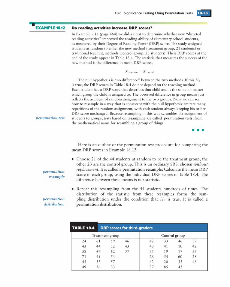
18.6 Significance Testing Using Permutation Tests 18-53
Do reading activities increase DRP scores?EXAMPLE18.12
�
�
permutation resample.
permutation distribution.
permutation tests,
Treatment group Control group
permutation test
permutationresample
permutationdistribution
0
treatment control
0
Here is an outline of the permutation test procedure for comparing themean DRP scores in Example 18.12:
Choose 21 of the 44 students at random to be the treatment group; theother 23 are the control group. This is an ordinary SRS, chosen
. It is called a Calculate the mean DRPscore in each group, using the individual DRP scores in Table 18.4. Thedifference between these means is our statistic.
Repeat this resampling from the 44 students hundreds of times. Thedistribution of the statistic from these resamples forms the sam-pling distribution under the condition that is true. It is called a
t
x x
H
withoutreplacement
H
In Example 7.11 (page 464) we did a test to determine whether new “directedreading activities” improved the reading ability of elementary school students,as measured by their Degree of Reading Power (DRP) score. The study assignedstudents at random to either the new method (treatment group, 21 students) ortraditional teaching methods (control group, 23 students). Their DRP scores at theend of the study appear in Table 18.4. The statistic that measures the success of thenew method is the difference in mean DRP scores,
The null hypothesis is “no difference” between the two methods. If thisis true, the DRP scores in Table 18.4 do not depend on the teaching method.Each student has a DRP score that describes that child and is the same no matterwhich group the child is assigned to. The observed difference in group means justreflects the accident of random assignment to the two groups. Now we can seehow to resample in a way that is consistent with the null hypothesis: imitate manyrepetitions of the random assignment, with each student always keeping his or herDRP score unchanged. Because resampling in this way scrambles the assignment ofstudents to groups, tests based on resampling are called fromthe mathematical name for scrambling a group of things.
24 61 59 46 42 33 46 3743 44 52 43 43 41 10 4258 67 62 57 55 19 17 5571 49 54 26 54 60 2843 53 57 62 20 53 4849 56 33 37 85 42
�
TABLE 18.4 DRP scores for third-graders

24, 61 | 42, 33, 46, 37x1 – x2 = 42.5 – 39.5 = 3.0
33, 61 | 24, 42, 46, 37x1 – x2 = 47 – 37.25 = 9.75
37, 42 | 24, 61, 33, 46x1 – x2 = 39.5 – 41 = –1.5
33, 46 | 24, 61, 42, 37x1 – x2 = 39.5 – 41 = –1.5
Bootstrap Methods and Permutation Tests18-54 CHAPTER 18
FIGURE 18.20
The permutation test for DRP scoresEXAMPLE18.13
�
�
The idea of permutation resampling. The top box shows the outcomes of a study with foursubjects in one group and two in the other. The boxes below show three permutation resamples. The valuesof the statistic for many such resamples form the permutation distribution.
a
� �� �treatment control
�0 treatment control
treatment control
The value of the statistic actually observed in the study was
51 476 41 522 9 954
Locate this value on the permutation distribution to get the -value.
Figure 18.20 illustrates permutation resampling on a small scale. Thetop box shows the results of a study with 4 subjects in the treatment groupand 2 subjects in the control group. A permutation resample chooses an SRSof 4 of the 6 subjects to form the treatment group. The remaining 2 are thecontrol group. The results of three permutation resamples appear belowthe original results, along with the statistic (difference in group means)for each.
H
H
P
P
P
x x . . .
P
Figure 18.21 shows the permutation distribution of the difference in means basedon 999 permutation resamples from the DRP data in Table 18.4. The solid line inthe figure marks the value of the statistic for the original sample, 9.954.
We seek evidence that the treatment increases DRP scores, so the hypotheses are
: 0
: 0
The -value for the one-sided test is the probability that the difference inmeans is 9.954 or greater, calculated taking the null hypothesis to be true. Thepermutation distribution in Figure 18.21 shows how the statistic would vary if thenull hypothesis were true. So the proportion of observations greater than 9.954estimates the -value. A look at the resampling results finds that 14 of the 999resamples gave a value of 9.954 or larger.
The proportion of samples that exceed the observed value 9.954 is 14/999, or0.014. Here is a last refinement. Recall from Chapter 8 that we can improve theestimate of a population proportion by adding two successes and two failures tothe sample. It turns out that we can similarly improve the estimate of the -value
�
� �
� �
� �

–15 –5–10 0 5 10 15
P-value
ObservedMean
18.6 Significance Testing Using Permutation Tests 18-55
FIGURE 18.21
Using software
The permutation distribution of the statisticbased on the DRP scores of 44 students. The
observed difference in means, 9.954, is in the right tail.treatment controlx x
permDRP = permutationTestMeans(data = DRP, treatment = group, alternative="greater")
plot(permDRP)permDRP
�
�
�� �
�
Figure 18.21 shows that the permutation distribution has a roughly Nor-mal shape. Because the permutation distribution approximates the samplingdistribution, we now know that the sampling distribution is close to Normal.When the sampling distribution is close to Normal, we can use the usualtwo-sample test. Example 7.11 shows that the test gives 0 013, veryclose to the -value from the permutation test.
In principle, you can program almost any statistical software to do apermutation test. It is much more convenient to use software that automatesthe process of resampling, calculating the statistic, forming the resamplingdistribution, and finding the -value.
The commands that do this in S-PLUS are
P
.
t t P .P
P
by adding one sample result above the observed statistic. The final permutation testestimate of the -value is
14 1 150 015
999 1 1000
The data give good evidence that the new method beats the standard method.
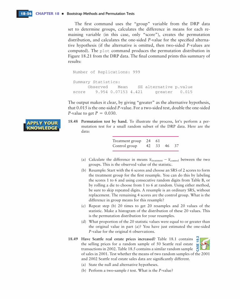
Bootstrap Methods and Permutation Tests18-56 CHAPTER 18 �
APPLY YOURKNOWLEDGE
plot
Number of Replications: 999
Summary Statistics:Observed Mean SE alternative p.value
score 9.954 0.07153 4.421 greater 0.015
18.48 Permutation test by hand.
18.49 Have Seattle real estate prices increased?
�
treatment control
The first command uses the “group” variable from the DRP dataset to determine groups, calculates the difference in means for each re-maining variable (in this case, only “score”), creates the permutationdistribution, and calculates the one-sided -value for the specified alterna-tive hypothesis (if the alternative is omitted, then two-sided -values arecomputed). The command produces the permutation distribution inFigure 18.21 from the DRP data. The final command prints this summary ofresults:
The output makes it clear, by giving “greater” as the alternative hypothesis,that 0.015 is the one-sided -value. For a two-sided test, double the one-sided
-value to get 0 030.
x x
P
t P
PP
PP P .
To illustrate the process, let’s perform a per-mutation test for a small random subset of the DRP data. Here are thedata:
Treatment group 24 61Control group 42 33 46 37
(a) Calculate the difference in means between the twogroups. This is the observed value of the statistic.
(b) Resample: Start with the 6 scores and choose an SRS of 2 scores to formthe treatment group for the first resample. You can do this by labelingthe scores 1 to 6 and using consecutive random digits from Table B, orby rolling a die to choose from 1 to 6 at random. Using either method,be sure to skip repeated digits. A resample is an ordinary SRS, withoutreplacement. The remaining 4 scores are the control group. What is thedifference in group means for this resample?
(c) Repeat step (b) 20 times to get 20 resamples and 20 values of thestatistic. Make a histogram of the distribution of these 20 values. Thisis the permutation distribution for your resamples.
(d) What proportion of the 20 statistic values were equal to or greater thanthe original value in part (a)? You have just estimated the one-sided
-value for the original 6 observations.
Table 18.1 containsthe selling prices for a random sample of 50 Seattle real estatetransactions in 2002. Table 18.5 contains a similar random sampleof sales in 2001. Test whether the means of two random samples of the 2001and 2002 Seattle real estate sales data are significantly different.
(a) State the null and alternative hypotheses.
(b) Perform a two-sample test. What is the -value?
�
CA
SE1
8.2
APPLY YOURKNOWLEDGE
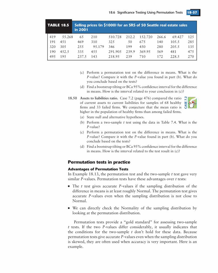
18.6 Significance Testing Using Permutation Tests 18-57
Advantages of Permutation Tests
�
�
Permutation tests in practice
18.50 Assets to liabilities ratio.
In Example 18.13, the permutation test and the two-sample test gave verysimilar -values. Permutation tests have these advantages over tests:
The test gives accurate -values if the sampling distribution of thedifference in means is at least roughly Normal. The permutation test givesaccurate -values even when the sampling distribution is not close toNormal.
We can directly check the Normality of the sampling distribution bylooking at the permutation distribution.
Permutation tests provide a “gold standard” for assessing two-sampletests. If the two -values differ considerably, it usually indicates that
the conditions for the two-sample don’t hold for these data. Becausepermutation tests give accurate -values even when the sampling distributionis skewed, they are often used when accuracy is very important. Here is anexample.
P P
tP
P P
tP t
t P
P
t Pt
P
419 55.268 65 210 510.728 212.2 152.720 266.6 69.427 125191 451 469 310 325 50 675 140 105.5 285320 305 255 95.179 346 199 450 280 205.5 135190 452.5 335 455 291.905 239.9 369.95 569 481 475495 195 237.5 143 218.95 239 710 172 228.5 270
(c) Perform a permutation test on the difference in means. What is the-value? Compare it with the -value you found in part (b). What do
you conclude based on the tests?
(d) Find a bootstrap tilting or BCa 95% confidence interval for the differencein means. How is the interval related to your conclusion in (c)?
Case 7.2 (page 476) compared the ratioof current assets to current liabilities for samples of 68 healthyfirms and 33 failed firms. We conjecture that the mean ratio ishigher in the population of healthy firms than among failed firms.
(a) State null and alternative hypotheses.
(b) Perform a two-sample test using the data in Table 7.4. What is the-value?
(c) Perform a permutation test on the difference in means. What is the-value? Compare it with the -value found in part (b). What do you
conclude based on the tests?
(d) Find a bootstrap tilting or BCa 95% confidence interval for the differencein means. How is the interval related to the test result in (c)?
CA
SE7
.2
TABLE 18.5 Selling prices (in $1000) for an SRS of 50 Seattle real estate salesin 2001
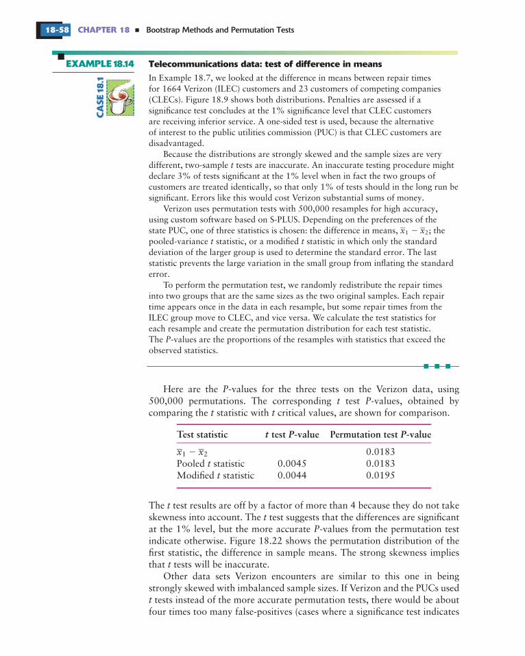
Bootstrap Methods and Permutation Tests18-58 CHAPTER 18
Telecommunications data: test of difference in meansEXAMPLE18.14
�
Test statistic test -value Permutation test -value
�1 2
1 2
Here are the -values for the three tests on the Verizon data, using500,000 permutations. The corresponding test -values, obtained bycomparing the statistic with critical values, are shown for comparison.
0.0183Pooled statistic 0.0045 0.0183Modified statistic 0.0044 0.0195
The test results are off by a factor of more than 4 because they do not takeskewness into account. The test suggests that the differences are significantat the 1% level, but the more accurate -values from the permutation testindicate otherwise. Figure 18.22 shows the permutation distribution of thefirst statistic, the difference in sample means. The strong skewness impliesthat tests will be inaccurate.
Other data sets Verizon encounters are similar to this one in beingstrongly skewed with imbalanced sample sizes. If Verizon and the PUCs used
tests instead of the more accurate permutation tests, there would be aboutfour times too many false-positives (cases where a significance test indicates
t
x xt t
P
Pt P
t t
x xt
t
tt
P
t
t
In Example 18.7, we looked at the difference in means between repair timesfor 1664 Verizon (ILEC) customers and 23 customers of competing companies(CLECs). Figure 18.9 shows both distributions. Penalties are assessed if asignificance test concludes at the 1% significance level that CLEC customersare receiving inferior service. A one-sided test is used, because the alternativeof interest to the public utilities commission (PUC) is that CLEC customers aredisadvantaged.
Because the distributions are strongly skewed and the sample sizes are verydifferent, two-sample tests are inaccurate. An inaccurate testing procedure mightdeclare 3% of tests significant at the 1% level when in fact the two groups ofcustomers are treated identically, so that only 1% of tests should in the long run besignificant. Errors like this would cost Verizon substantial sums of money.
Verizon uses permutation tests with 500,000 resamples for high accuracy,using custom software based on S-PLUS. Depending on the preferences of thestate PUC, one of three statistics is chosen: the difference in means, ; thepooled-variance statistic, or a modified statistic in which only the standarddeviation of the larger group is used to determine the standard error. The laststatistic prevents the large variation in the small group from inflating the standarderror.
To perform the permutation test, we randomly redistribute the repair timesinto two groups that are the same sizes as the two original samples. Each repairtime appears once in the data in each resample, but some repair times from theILEC group move to CLEC, and vice versa. We calculate the test statistics foreach resample and create the permutation distribution for each test statistic.The -values are the proportions of the resamples with statistics that exceed theobserved statistics.
t P P
�
CA
SE18
.1
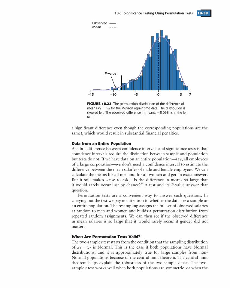
–15 –10 –5 0 5 7
ObservedMean
P-value
18.6 Significance Testing Using Permutation Tests 18-59
FIGURE 18.22
Data from an Entire Population
When Are Permutation Tests Valid?
The permutation distribution of the difference ofmeans for the Verizon repair time data. The distribution isskewed left. The observed difference in means, 8 098, is in the lefttail.
1 2x x.
�1 2
��
a significant difference even though the corresponding populations are thesame), which would result in substantial financial penalties.
A subtle difference between confidence intervals and significance tests is thatconfidence intervals require the distinction between sample and populationbut tests do not. If we have data on an entire population—say, all employeesof a large corporation—we don’t need a confidence interval to estimate thedifference between the mean salaries of male and female employees. We cancalculate the means for all men and for all women and get an exact answer.But it still makes sense to ask, “Is the difference in means so large thatit would rarely occur just by chance?” A test and its -value answer thatquestion.
Permutation tests are a convenient way to answer such questions. Incarrying out the test we pay no attention to whether the data are a sample oran entire population. The resampling assigns the full set of observed salariesat random to men and women and builds a permutation distribution fromrepeated random assignments. We can then see if the observed differencein mean salaries is so large that it would rarely occur if gender did notmatter.
The two-sample test starts from the condition that the sampling distributionof is Normal. This is the case if both populations have Normaldistributions, and it is approximately true for large samples from non-Normal populations because of the central limit theorem. The central limittheorem helps explain the robustness of the two-sample test. The two-sample test works well when both populations are symmetric, or when the
P
tx x
tt
Bootstrap Methods and Permutation Tests18-60 CHAPTER 18
Sources of Variation
�
APPLY YOURKNOWLEDGE
18.51 Choosing the number of resamples.
18.52 Validity of test methods.
��
1 2
populations have mild skewness in the same direction and the two samplesizes are similar.
The permutation test completely removes the Normality condition. Thetradeoff is that it requires the two populations to have identical distributionswhen the null hypothesis is true—not only the same means, but also the samespreads and shapes. It needs this to be able to move observations randomlybetween groups. In practice it is robust against different distributions, exceptfor different spreads when the sample sizes are not similar. Our preferredversion of the two-sample allows different standard deviations in the twopopulations.
However, this is rarely a reason to choose the test over the permutationtest, for two reasons. First, even if you notice that the two samples havedifferent standard deviations, this does not necessarily mean that the pop-ulation standard deviations differ. Particularly for skewed populations, thesample standard deviations may be very different even when the populationstandard deviations are the same. Second, it is usually reasonable to assumethat the distributions are approximately the same if the null hypothesisis true. In practice robustness against unequal standard deviations is lessimportant for hypothesis testing than for confidence intervals.
In Example 18.14, the distributions are strongly skewed, ruling out thetest. The permutation test is valid if the repair time distributions for
Verizon customers and CLEC customers are the same if the null hypothesisis true—in other words, that all customers are treated the same.
Just as in the case of bootstrap confidence intervals, permutation tests aresubject to two sources of random variability: the original sample is chosen atrandom from the population, and the resamples are chosen at random fromthe sample. Again as in the case of the bootstrap, the added variation due toresampling is usually small and can be made as small as we like by increasingthe number of resamples. For example, Verizon uses 500,000 resamples.
For most purposes, 999 resamples are sufficient. If stakes are high or-values are near a critical value (for example, near 0.01 in the Verizon
example), increase the number of resamples. Here is a helpful guideline: Ifthe true (one-sided) -value is , the standard deviation of the estimated
-value is approximately (1 )/ , where is the number of resamples.You can choose to obtain a desired level of accuracy.
P
P x x
P PP p
t
t
t
t
t
t
P
P pP p p B B
B
The estimated -value for the DRPstudy (Example 18.13) based on 999 resamples is 0.015. For the Verizonstudy (Example 18.14) the estimated -value for the test based onis 0.0183 based on 500,000 resamples. What is the approximate standarddeviation of each of these estimated -values? (Use each as an estimate ofthe unknown true -value .)
You want to test the equality of the means of twopopulations. Sketch density curves for two populations for which
(a) a permutation test is valid but a test is not.
(b) both permutation and tests are valid.
(c) a test is valid but a permutation test is not.
�
APPLY YOURKNOWLEDGE
18.6 Significance Testing Using Permutation Tests 18-61
Permutation Test for Matched Pairs
Effects of language instructionEXAMPLE18.15
Permutation tests in other settings
GENERAL PROCEDURE FOR PERMUTATION TESTS
�
���
�1 2
2 21 2 1 21 2
The bootstrap procedure can replace many different formula-based confi-dence intervals, provided that we resample in a way that matches the setting.The permutation test is also a general method that can be adapted to varioussettings.
To carry out a permutation test based on a statistic that measures thesize of an effect of interest:
1. Compute the statistic for the original data.
2. Choose permutation resamples from the data withoutreplacement in a way that is consistent with the null hypothesisof the test and with the study design. Construct the permutationdistribution of the statistic from its values in a large number ofresamples.
3. Find the -value by locating the original statistic on thepermutation distribution.
Formula methods generally obtain -values from a standard distributionsuch as or , using either tables or software algorithms. The test statisticmust be standardized so that it has the required distribution when the nullhypothesis is true. This is why the two-sample test uses ( )/
( / ) ( / ) rather than the simpler . Permutation tests, incontrast, generate a sampling distribution on the fly from the data and thechosen statistic. This allows greater flexibility in the choice of statistic inStep 1 of the procedure.
The key step in the general procedure for permutation tests is to formpermutation resamples in a way that is consistent with the study designand with the null hypothesis. Our examples and exercises to this point haveconcerned two-sample settings. How must we modify our procedure for amatched pairs design?
P
Pt F
t t x xs n s n x x
Example 7.7 (page 443) looked at scores of 20 executives on a French languagelistening test taken both before and after a language course. The “before” and“after” data are not two independent samples, because each executive’s scoresreflect his or her previous knowledge of French and other individual factors. Thescores appear in Table 7.2. How shall we carry out a permutation test?
The null hypothesis says that the language course has no effect on test scores. Ifthis is true, each executive’s before and after scores are just two measurements of thatperson’s understanding of French. The “before” and “after” have no meaning becausethe course has no effect. Resampling randomly assigns one of each executive’s twoscores to “before” and the other to “after.” We do not mix scores from differentpeople because that isn’t consistent with the pairing in the study design.
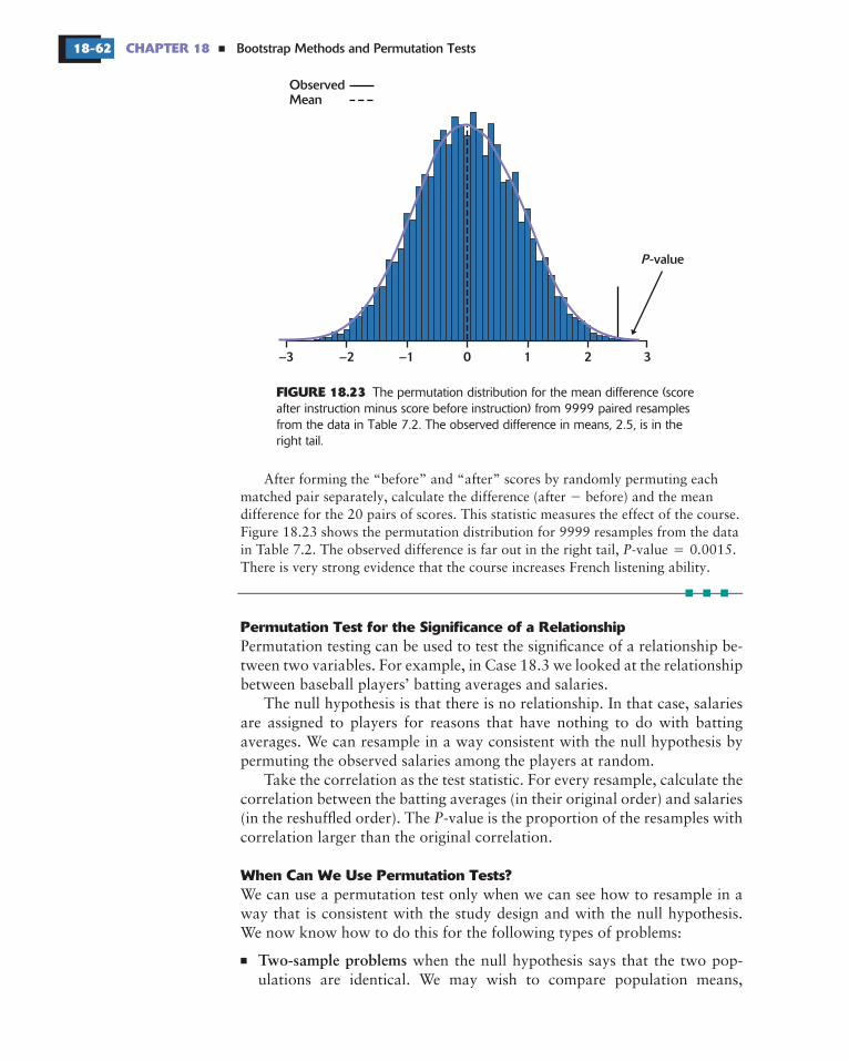
–3 –2 –1 0 1 2 3
P-value
ObservedMean
Bootstrap Methods and Permutation Tests18-62 CHAPTER 18
FIGURE 18.23
Permutation Test for the Significance of a Relationship
When Can We Use Permutation Tests?
�
�
The permutation distribution for the mean difference (scoreafter instruction minus score before instruction) from 9999 paired resamplesfrom the data in Table 7.2. The observed difference in means, 2.5, is in theright tail.
Two-sample problems
�
Permutation testing can be used to test the significance of a relationship be-tween two variables. For example, in Case 18.3 we looked at the relationshipbetween baseball players’ batting averages and salaries.
The null hypothesis is that there is no relationship. In that case, salariesare assigned to players for reasons that have nothing to do with battingaverages. We can resample in a way consistent with the null hypothesis bypermuting the observed salaries among the players at random.
Take the correlation as the test statistic. For every resample, calculate thecorrelation between the batting averages (in their original order) and salaries(in the reshuffled order). The -value is the proportion of the resamples withcorrelation larger than the original correlation.
We can use a permutation test only when we can see how to resample in away that is consistent with the study design and with the null hypothesis.We now know how to do this for the following types of problems:
when the null hypothesis says that the two pop-ulations are identical. We may wish to compare population means,
P .
P
After forming the “before” and “after” scores by randomly permuting eachmatched pair separately, calculate the difference (after before) and the meandifference for the 20 pairs of scores. This statistic measures the effect of the course.Figure 18.23 shows the permutation distribution for 9999 resamples from the datain Table 7.2. The observed difference is far out in the right tail, -value 0 0015.There is very strong evidence that the course increases French listening ability.
�
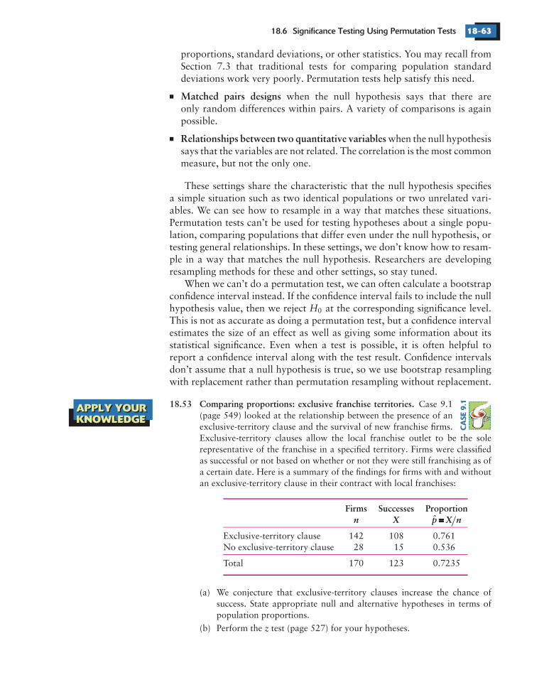
18.6 Significance Testing Using Permutation Tests 18-63
�
�
APPLY YOURKNOWLEDGE
Matched pairs designs
Relationships between two quantitative variables
18.53 Comparing proportions: exclusive franchise territories.
Firms Successes Proportionˆ ==========n X p ===== X n
0
�
proportions, standard deviations, or other statistics. You may recall fromSection 7.3 that traditional tests for comparing population standarddeviations work very poorly. Permutation tests help satisfy this need.
when the null hypothesis says that there areonly random differences within pairs. A variety of comparisons is againpossible.
when the null hypothesissays that the variables are not related. The correlation is the most commonmeasure, but not the only one.
These settings share the characteristic that the null hypothesis specifiesa simple situation such as two identical populations or two unrelated vari-ables. We can see how to resample in a way that matches these situations.Permutation tests can’t be used for testing hypotheses about a single popu-lation, comparing populations that differ even under the null hypothesis, ortesting general relationships. In these settings, we don’t know how to resam-ple in a way that matches the null hypothesis. Researchers are developingresampling methods for these and other settings, so stay tuned.
When we can’t do a permutation test, we can often calculate a bootstrapconfidence interval instead. If the confidence interval fails to include the nullhypothesis value, then we reject at the corresponding significance level.This is not as accurate as doing a permutation test, but a confidence intervalestimates the size of an effect as well as giving some information about itsstatistical significance. Even when a test is possible, it is often helpful toreport a confidence interval along with the test result. Confidence intervalsdon’t assume that a null hypothesis is true, so we use bootstrap resamplingwith replacement rather than permutation resampling without replacement.
z
H
Case 9.1(page 549) looked at the relationship between the presence of anexclusive-territory clause and the survival of new franchise firms.Exclusive-territory clauses allow the local franchise outlet to be the solerepresentative of the franchise in a specified territory. Firms were classifiedas successful or not based on whether or not they were still franchising as ofa certain date. Here is a summary of the findings for firms with and withoutan exclusive-territory clause in their contract with local franchises:
Exclusive-territory clause 142 108 0.761No exclusive-territory clause 28 15 0.536
Total 170 123 0.7235
(a) We conjecture that exclusive-territory clauses increase the chance ofsuccess. State appropriate null and alternative hypotheses in terms ofpopulation proportions.
(b) Perform the test (page 527) for your hypotheses.
CA
SE9
.1APPLY YOURKNOWLEDGE

Bootstrap Methods and Permutation Tests18-64 CHAPTER 18
ECTION UMMARY
�
�
�
�
�
S 18.6 SPermutation tests permutation resamples
without replacement
two-sample design
matchedpairs
no relationship
permutation distribution
18.54 Matched pairs: designing controls.
18.55 Correlation: salary and batting average.
1 2
are significance tests based ondrawn at random from the original data. Permutation resamples are drawn
, in contrast to bootstrap samples, which are drawnwith replacement.
Permutation resamples must be drawn in a way that is consistent withthe null hypothesis and with the study design. In a , thenull hypothesis says that the two populations are identical. Resamplingrandomly reassigns observations to the two groups. In a
design, randomly permute the two observations within each pairseparately. To test the hypothesis of between two variables,randomly reassign values of one of the two variables.
The of a suitable statistic is formed by thevalues of the statistic in a large number of resamples. Find the -value ofthe test by locating the original value of the statistic on the permutationdistribution.
When they can be used, permutation tests have great advantages. Theydo not require specific population shapes such as Normality. They apply toa variety of statistics, not just to statistics that have a simple distribution
p p
P
P
P
P
P
(c) Perform a permutation test based on the difference in the sampleˆ ˆproportions . Explain carefully how the resampling is consistent
with the null hypothesis. Compare your result with part (b).
(d) Based on your permutation test -value, what do you conclude aboutthe effect of exclusive-territory clauses?
(e) Give a bootstrap tilting or BCa interval for the difference between thetwo population proportions. Explain how the interval is consistent withthe permutation test.
Exercise 7.40 (page 458) describes astudy in which 25 right-handed subjects were asked to turn a knob clockwiseand counterclockwise (in random order). The response variable is the timeneeded to move an indicator a fixed distance. We conjecture that clockwisemovement is easier for right-handed people.
(a) State null and alternative hypotheses in terms of mean times. Carefullyidentify the parameters in your hypotheses.
(b) Perform a matched pairs permutation test. What is the -value? Whatdo you conclude about designing controls?
(c) Graph the permutation distribution and indicate the region that corre-sponds to the -value.
Table 18.2 contains thesalaries and batting averages of a random sample of 50 majorleague baseball players. We wonder if these variables are correlatedin the population of all players.
(a) State the null and alternative hypotheses.
(b) Perform a permutation test based on the sample correlation. Report the-value and draw a conclusion.
�
CA
SE1
8.3
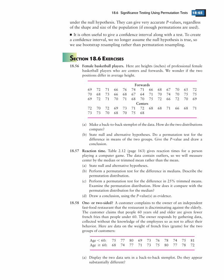
18.6 Significance Testing Using Permutation Tests 18-65
ECTION XERCISES
�
S 18.6 E18.56 Female basketball players.
Forwards
Centers
18.57 Reaction time.
18.58 One- or two-sided?
under the null hypothesis. They can give very accurate -values, regardlessof the shape and size of the population (if enough permutations are used).
It is often useful to give a confidence interval along with a test. To createa confidence interval, we no longer assume the null hypothesis is true, sowe use bootstrap resampling rather than permutation resampling.
P
P
P
Here are heights (inches) of professional femalebasketball players who are centers and forwards. We wonder if the twopositions differ in average height.
69 72 71 66 76 74 71 66 68 67 70 65 7270 68 73 66 68 67 64 71 70 74 70 75 7569 72 71 70 71 68 70 75 72 66 72 70 69
72 70 72 69 73 71 72 68 68 71 66 68 7173 73 70 68 70 75 68
(a) Make a back-to-back stemplot of the data. How do the two distributionscompare?
(b) State null and alternative hypotheses. Do a permutation test for thedifference in means of the two groups. Give the -value and draw aconclusion.
Table 2.12 (page 163) gives reaction times for a personplaying a computer game. The data contain outliers, so we will measurecenter by the median or trimmed mean rather than the mean.
(a) State null and alternative hypotheses.
(b) Perform a permutation test for the difference in medians. Describe thepermutation distribution.
(c) Perform a permutation test for the difference in 25% trimmed means.Examine the permutation distribution. How does it compare with thepermutation distribution for the median?
(d) Draw a conclusion, using the -value(s) as evidence.
A customer complains to the owner of an independentfast-food restaurant that the restaurant is discriminating against the elderly.The customer claims that people 60 years old and older are given fewerfrench fries than people under 60. The owner responds by gathering data,collected without the knowledge of the employees so as not to affect theirbehavior. Here are data on the weight of french fries (grams) for the twogroups of customers:
Age 60: 75 77 80 69 73 76 78 74 75 81Age 60: 68 74 77 71 73 75 80 77 78 72
(a) Display the two data sets in a back-to-back stemplot. Do they appearsubstantially different?
�
�
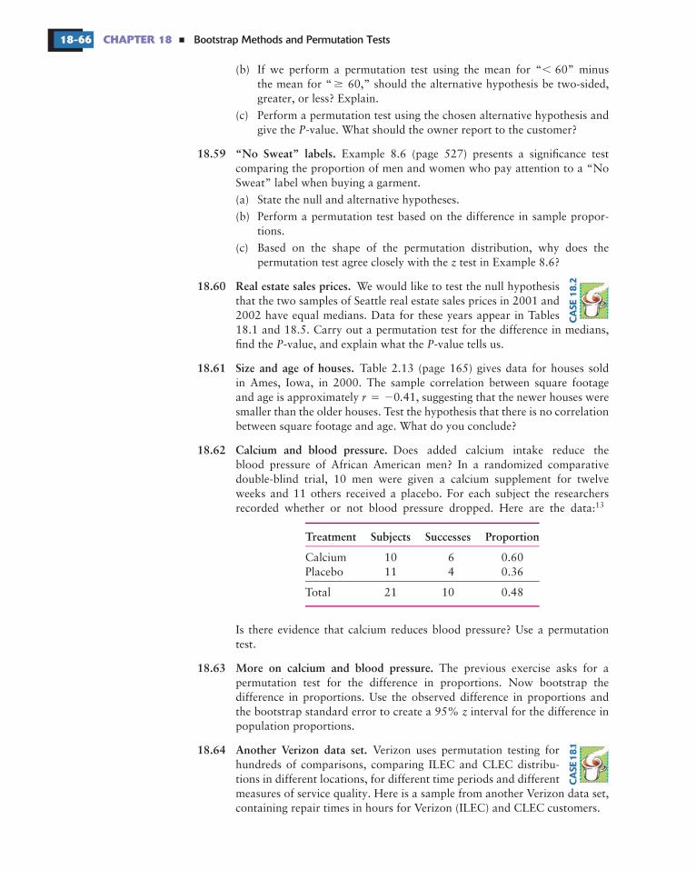
Bootstrap Methods and Permutation Tests18-66 CHAPTER 18 �
18.59 “No Sweat” labels.
18.60 Real estate sales prices.
18.61 Size and age of houses.
18.62 Calcium and blood pressure.
Treatment Subjects Successes Proportion
18.63 More on calcium and blood pressure.
18.64 Another Verizon data set.
�
13
P
z
P P
r .
z
(b) If we perform a permutation test using the mean for “ 60” minusthe mean for “ 60,” should the alternative hypothesis be two-sided,greater, or less? Explain.
(c) Perform a permutation test using the chosen alternative hypothesis andgive the -value. What should the owner report to the customer?
Example 8.6 (page 527) presents a significance testcomparing the proportion of men and women who pay attention to a “NoSweat” label when buying a garment.
(a) State the null and alternative hypotheses.
(b) Perform a permutation test based on the difference in sample propor-tions.
(c) Based on the shape of the permutation distribution, why does thepermutation test agree closely with the test in Example 8.6?
We would like to test the null hypothesisthat the two samples of Seattle real estate sales prices in 2001 and2002 have equal medians. Data for these years appear in Tables18.1 and 18.5. Carry out a permutation test for the difference in medians,find the -value, and explain what the -value tells us.
Table 2.13 (page 165) gives data for houses soldin Ames, Iowa, in 2000. The sample correlation between square footageand age is approximately 0 41, suggesting that the newer houses weresmaller than the older houses. Test the hypothesis that there is no correlationbetween square footage and age. What do you conclude?
Does added calcium intake reduce theblood pressure of African American men? In a randomized comparativedouble-blind trial, 10 men were given a calcium supplement for twelveweeks and 11 others received a placebo. For each subject the researchersrecorded whether or not blood pressure dropped. Here are the data:
Calcium 10 6 0.60Placebo 11 4 0.36
Total 21 10 0.48
Is there evidence that calcium reduces blood pressure? Use a permutationtest.
The previous exercise asks for apermutation test for the difference in proportions. Now bootstrap thedifference in proportions. Use the observed difference in proportions andthe bootstrap standard error to create a 95% interval for the difference inpopulation proportions.
Verizon uses permutation testing forhundreds of comparisons, comparing ILEC and CLEC distribu-tions in different locations, for different time periods and differentmeasures of service quality. Here is a sample from another Verizon data set,containing repair times in hours for Verizon (ILEC) and CLEC customers.
�
�
�
CA
SE1
8.2
CA
SE1
8.1
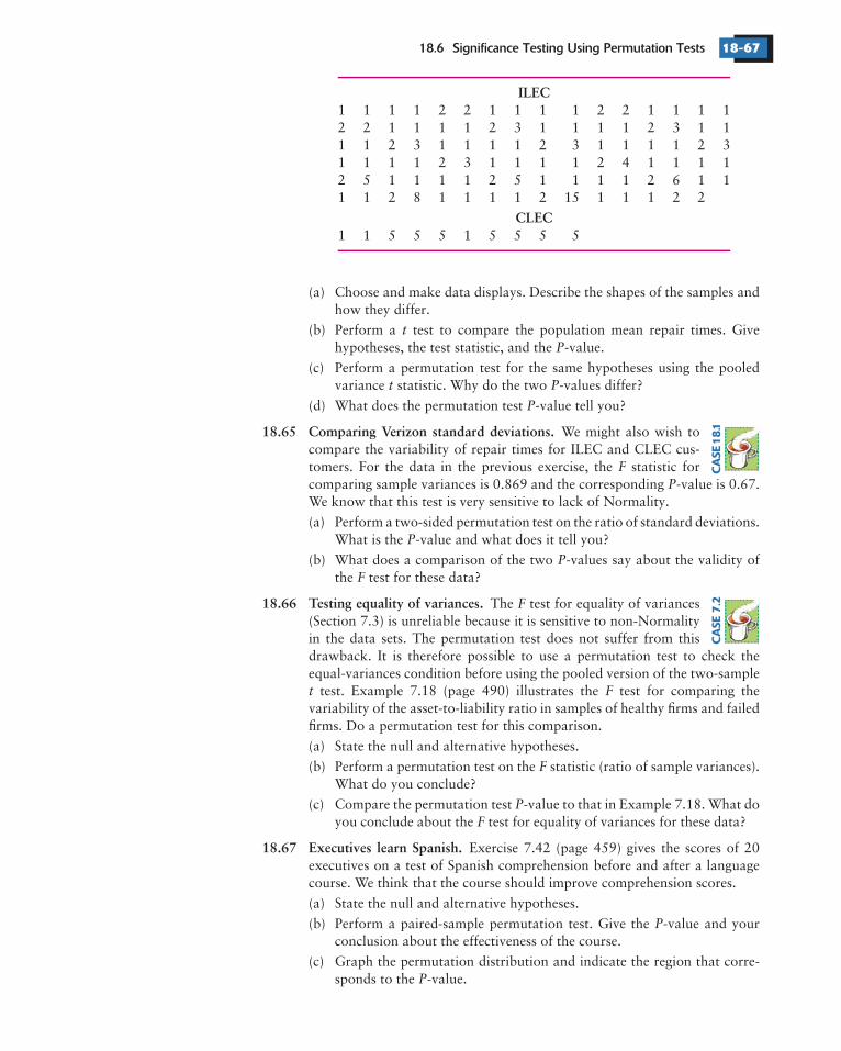
18.6 Significance Testing Using Permutation Tests 18-67
ILEC
CLEC
18.65 Comparing Verizon standard deviations.
18.66 Testing equality of variances.
18.67 Executives learn Spanish.
tP
t P
P
FP
P
PF
F
t F
F
PF
P
P
1 1 1 1 2 2 1 1 1 1 2 2 1 1 1 12 2 1 1 1 1 2 3 1 1 1 1 2 3 1 11 1 2 3 1 1 1 1 2 3 1 1 1 1 2 31 1 1 1 2 3 1 1 1 1 2 4 1 1 1 12 5 1 1 1 1 2 5 1 1 1 1 2 6 1 11 1 2 8 1 1 1 1 2 15 1 1 1 2 2
1 1 5 5 5 1 5 5 5 5
(a) Choose and make data displays. Describe the shapes of the samples andhow they differ.
(b) Perform a test to compare the population mean repair times. Givehypotheses, the test statistic, and the -value.
(c) Perform a permutation test for the same hypotheses using the pooledvariance statistic. Why do the two -values differ?
(d) What does the permutation test -value tell you?
We might also wish tocompare the variability of repair times for ILEC and CLEC cus-tomers. For the data in the previous exercise, the statistic forcomparing sample variances is 0.869 and the corresponding -value is 0.67.We know that this test is very sensitive to lack of Normality.
(a) Perform a two-sided permutation test on the ratio of standard deviations.What is the -value and what does it tell you?
(b) What does a comparison of the two -values say about the validity ofthe test for these data?
The test for equality of variances(Section 7.3) is unreliable because it is sensitive to non-Normalityin the data sets. The permutation test does not suffer from thisdrawback. It is therefore possible to use a permutation test to check theequal-variances condition before using the pooled version of the two-sample
test. Example 7.18 (page 490) illustrates the test for comparing thevariability of the asset-to-liability ratio in samples of healthy firms and failedfirms. Do a permutation test for this comparison.
(a) State the null and alternative hypotheses.
(b) Perform a permutation test on the statistic (ratio of sample variances).What do you conclude?
(c) Compare the permutation test -value to that in Example 7.18. What doyou conclude about the test for equality of variances for these data?
Exercise 7.42 (page 459) gives the scores of 20executives on a test of Spanish comprehension before and after a languagecourse. We think that the course should improve comprehension scores.
(a) State the null and alternative hypotheses.
(b) Perform a paired-sample permutation test. Give the -value and yourconclusion about the effectiveness of the course.
(c) Graph the permutation distribution and indicate the region that corre-sponds to the -value.
CA
SE7
.2C
ASE
18
.1
Bootstrap Methods and Permutation Tests18-68 CHAPTER 18
TATISTICS IN UMMARY
HAPTER EVIEW XERCISES
�
S
C
S
18 R E
A. BOOTSTRAP
B. PERMUTATION TESTS
18.68 Piano lessons.
Fast and inexpensive computing power allows the use of statistical proce-dures that require large-scale computation. Bootstrap confidence intervalsand permutation tests are based on large numbers of “resamples” drawnfrom the data. These resampling computations replace the formulas derivedfrom probability theory that we use in traditional confidence intervals andtests. Resampling procedures can often be used in settings that do not meetthe conditions for use of formula-based procedures. These resampling pro-cedures are becoming ever more common in statistical practice. It is possiblethat in the future they will largely replace some traditional procedures.Reading this chapter should enable you to do the following:
1. Explain the bootstrap resampling idea in the context of a particulardata set used to estimate a particular population parameter.
2. Use software such as S-PLUS to bootstrap a statistic of your choicefrom a set of data. Plot the bootstrap distribution and obtain thebootstrap standard error and the bootstrap estimate of bias.
3. Based on bootstrap software output, judge whether formula-basedconfidence intervals that require Normal sampling distributions canbe used and whether the simple bootstrap and percentile confidenceintervals can be used.
4. Obtain from bootstrap software output any of the four types ofbootstrap confidence intervals for a parameter: , percentile, BCa, andtilting. By comparing these intervals judge which are safe to use.
1. Recognize the settings in which we can use permutation tests. Insuch a setting, explain how to choose permutation resamples that areconsistent with the null hypothesis and with the design of the study.
2. Use software to obtain the permutation distribution of a test statistic ofyour choice in settings that allow permutation tests. Give the -valueof the test.
3. Based on permutation test software output, judge whether a traditionalformula-based test can be used.
t
t
P
Exercise 7.34 (page 456) reports the changes in reasoningscores of 34 preschool children after six months of piano lessons. Here arethe changes:
2 5 7 2 2 7 4 1 0 7 3 4 3 4 9 4 52 9 6 0 3 6 1 3 4 6 7 2 7 3 3 4 4
(a) Make a histogram and Normal quantile plot of the data. Is the distribu-tion approximately Normal?
�
� � �
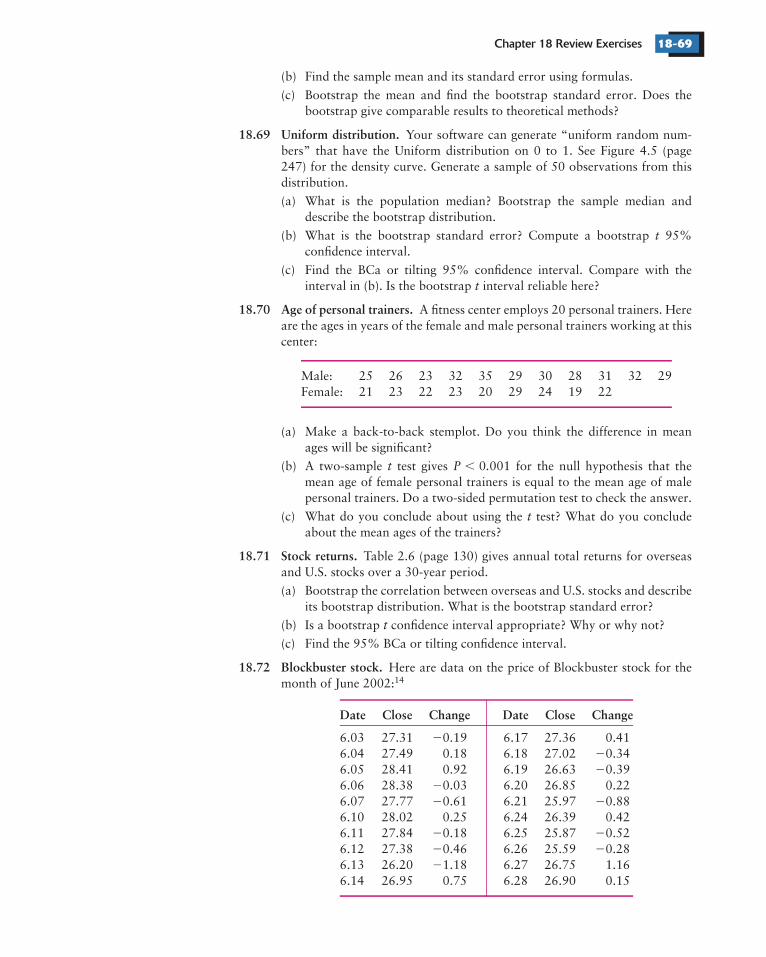
Chapter 18 Review Exercises 18-69
18.69 Uniform distribution.
18.70 Age of personal trainers.
18.71 Stock returns.
18.72 Blockbuster stock.
Date Close Change Date Close Change
14
t
t
t P .
t
t
(b) Find the sample mean and its standard error using formulas.
(c) Bootstrap the mean and find the bootstrap standard error. Does thebootstrap give comparable results to theoretical methods?
Your software can generate “uniform random num-bers” that have the Uniform distribution on 0 to 1. See Figure 4.5 (page247) for the density curve. Generate a sample of 50 observations from thisdistribution.
(a) What is the population median? Bootstrap the sample median anddescribe the bootstrap distribution.
(b) What is the bootstrap standard error? Compute a bootstrap 95%confidence interval.
(c) Find the BCa or tilting 95% confidence interval. Compare with theinterval in (b). Is the bootstrap interval reliable here?
A fitness center employs 20 personal trainers. Hereare the ages in years of the female and male personal trainers working at thiscenter:
Male: 25 26 23 32 35 29 30 28 31 32 29Female: 21 23 22 23 20 29 24 19 22
(a) Make a back-to-back stemplot. Do you think the difference in meanages will be significant?
(b) A two-sample test gives 0 001 for the null hypothesis that themean age of female personal trainers is equal to the mean age of malepersonal trainers. Do a two-sided permutation test to check the answer.
(c) What do you conclude about using the test? What do you concludeabout the mean ages of the trainers?
Table 2.6 (page 130) gives annual total returns for overseasand U.S. stocks over a 30-year period.
(a) Bootstrap the correlation between overseas and U.S. stocks and describeits bootstrap distribution. What is the bootstrap standard error?
(b) Is a bootstrap confidence interval appropriate? Why or why not?
(c) Find the 95% BCa or tilting confidence interval.
Here are data on the price of Blockbuster stock for themonth of June 2002:
6.03 27.31 0.19 6.17 27.36 0.416.04 27.49 0.18 6.18 27.02 0.346.05 28.41 0.92 6.19 26.63 0.396.06 28.38 0.03 6.20 26.85 0.226.07 27.77 0.61 6.21 25.97 0.886.10 28.02 0.25 6.24 26.39 0.426.11 27.84 0.18 6.25 25.87 0.526.12 27.38 0.46 6.26 25.59 0.286.13 26.20 1.18 6.27 26.75 1.166.14 26.95 0.75 6.28 26.90 0.15
�
�
�
�
�
� �
� �
� �
�
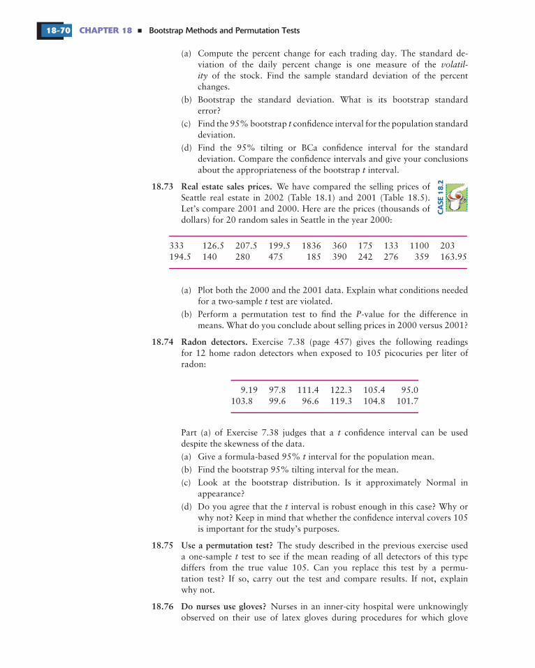
Bootstrap Methods and Permutation Tests18-70 CHAPTER 18 �
18.73 Real estate sales prices.
18.74 Radon detectors.
18.75 Use a permutation test?
18.76 Do nurses use gloves?
volatil-ity
t
t
t
P
t
t
t
t
(a) Compute the percent change for each trading day. The standard de-viation of the daily percent change is one measure of the
of the stock. Find the sample standard deviation of the percentchanges.
(b) Bootstrap the standard deviation. What is its bootstrap standarderror?
(c) Find the 95% bootstrap confidence interval for the population standarddeviation.
(d) Find the 95% tilting or BCa confidence interval for the standarddeviation. Compare the confidence intervals and give your conclusionsabout the appropriateness of the bootstrap interval.
We have compared the selling prices ofSeattle real estate in 2002 (Table 18.1) and 2001 (Table 18.5).Let’s compare 2001 and 2000. Here are the prices (thousands ofdollars) for 20 random sales in Seattle in the year 2000:
333 126.5 207.5 199.5 1836 360 175 133 1100 203194.5 140 280 475 185 390 242 276 359 163.95
(a) Plot both the 2000 and the 2001 data. Explain what conditions neededfor a two-sample test are violated.
(b) Perform a permutation test to find the -value for the difference inmeans. What do you conclude about selling prices in 2000 versus 2001?
Exercise 7.38 (page 457) gives the following readingsfor 12 home radon detectors when exposed to 105 picocuries per liter ofradon:
9.19 97.8 111.4 122.3 105.4 95.0103.8 99.6 96.6 119.3 104.8 101.7
Part (a) of Exercise 7.38 judges that a confidence interval can be useddespite the skewness of the data.
(a) Give a formula-based 95% interval for the population mean.
(b) Find the bootstrap 95% tilting interval for the mean.
(c) Look at the bootstrap distribution. Is it approximately Normal inappearance?
(d) Do you agree that the interval is robust enough in this case? Why orwhy not? Keep in mind that whether the confidence interval covers 105is important for the study’s purposes.
The study described in the previous exercise useda one-sample test to see if the mean reading of all detectors of this typediffers from the true value 105. Can you replace this test by a permu-tation test? If so, carry out the test and compare results. If not, explainwhy not.
Nurses in an inner-city hospital were unknowinglyobserved on their use of latex gloves during procedures for which glove
CA
SE1
8.2
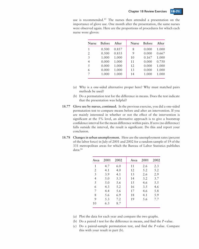
Chapter 18 Review Exercises 18-71
Nurse Before After Nurse Before After
18.77 Glove use by nurses, continued.
18.78 Changes in urban unemployment.
Area 2001 2002 Area 2001 2002
15
16
t P
P
use is recommended. The nurses then attended a presentation on theimportance of glove use. One month after the presentation, the same nurseswere observed again. Here are the proportions of procedures for which eachnurse wore gloves:
1 0.500 0.857 8 0.000 1.0002 0.500 0.833 9 0.000 0.6673 1.000 1.000 10 0.167 1.0004 0.000 1.000 11 0.000 0.7505 0.000 1.000 12 0.000 1.0006 0.000 1.000 13 0.000 1.0007 1.000 1.000 14 1.000 1.000
(a) Why is a one-sided alternative proper here? Why must matched pairsmethods be used?
(b) Do a permutation test for the difference in means. Does the test indicatethat the presentation was helpful?
In the previous exercise, you did a one-sidedpermutation test to compare means before and after an intervention. If youare mainly interested in whether or not the effect of the intervention issignificant at the 5% level, an alternative approach is to give a bootstrapconfidence interval for the mean difference within pairs. If zero (no difference)falls outside the interval, the result is significant. Do this and report yourconclusion.
Here are the unemployment rates (percentof the labor force) in July of 2001 and 2002 for a random sample of 19 of the331 metropolitan areas for which the Bureau of Labor Statistics publishesdata:
1 4.7 6.0 11 2.6 2.32 4.1 4.0 12 5.2 5.23 3.9 4.1 13 2.6 2.94 5.0 5.3 14 3.2 3.75 5.0 5.6 15 4.6 5.56 4.3 5.2 16 3.5 4.67 4.4 5.6 17 4.6 5.88 5.6 6.9 18 4.1 5.99 5.3 7.2 19 5.6 7.7
10 6.3 8.7
(a) Plot the data for each year and compare the two graphs.
(b) Do a paired test for the difference in means, and find the -value.
(c) Do a paired-sample permutation test, and find the -value. Comparethis with your result in part (b).
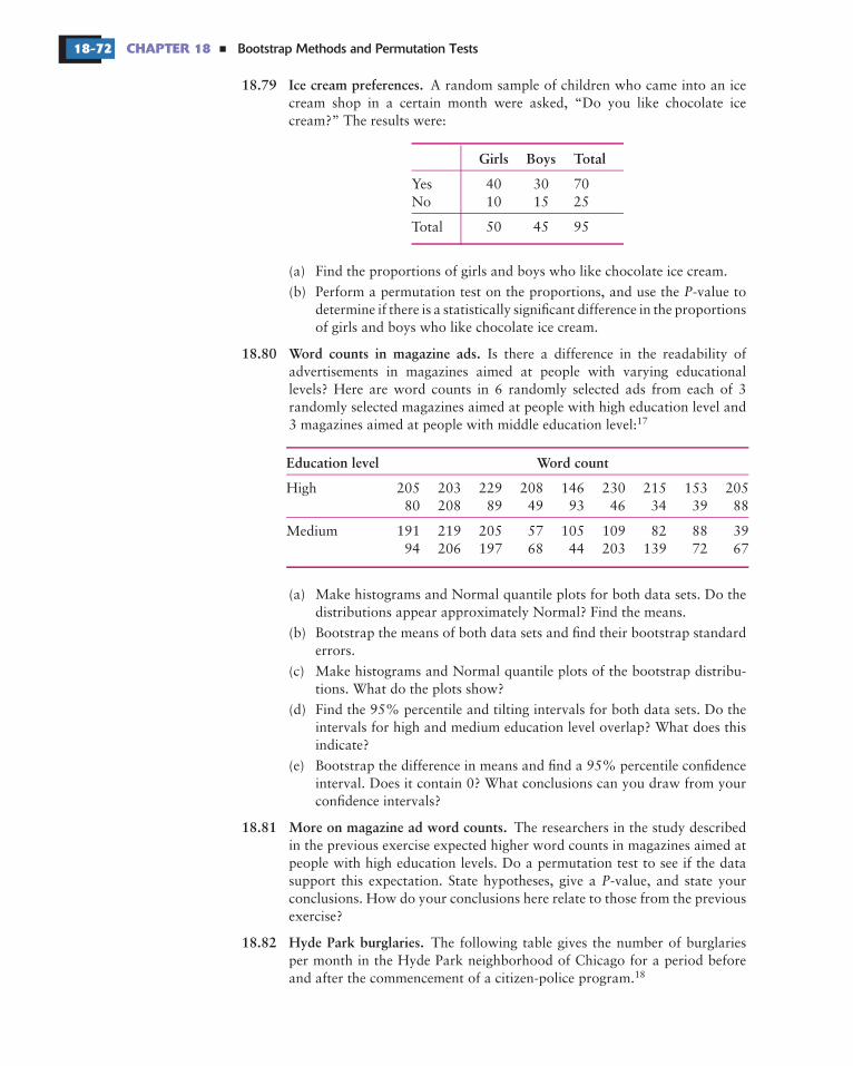
Bootstrap Methods and Permutation Tests18-72 CHAPTER 18 �
18.79 Ice cream preferences.
Girls Boys Total
18.80 Word counts in magazine ads.
Education level Word count
18.81 More on magazine ad word counts.
18.82 Hyde Park burglaries.
17
18
P
P
A random sample of children who came into an icecream shop in a certain month were asked, “Do you like chocolate icecream?” The results were:
Yes 40 30 70No 10 15 25
Total 50 45 95
(a) Find the proportions of girls and boys who like chocolate ice cream.
(b) Perform a permutation test on the proportions, and use the -value todetermine if there is a statistically significant difference in the proportionsof girls and boys who like chocolate ice cream.
Is there a difference in the readability ofadvertisements in magazines aimed at people with varying educationallevels? Here are word counts in 6 randomly selected ads from each of 3randomly selected magazines aimed at people with high education level and3 magazines aimed at people with middle education level:
High 205 203 229 208 146 230 215 153 20580 208 89 49 93 46 34 39 88
Medium 191 219 205 57 105 109 82 88 3994 206 197 68 44 203 139 72 67
(a) Make histograms and Normal quantile plots for both data sets. Do thedistributions appear approximately Normal? Find the means.
(b) Bootstrap the means of both data sets and find their bootstrap standarderrors.
(c) Make histograms and Normal quantile plots of the bootstrap distribu-tions. What do the plots show?
(d) Find the 95% percentile and tilting intervals for both data sets. Do theintervals for high and medium education level overlap? What does thisindicate?
(e) Bootstrap the difference in means and find a 95% percentile confidenceinterval. Does it contain 0? What conclusions can you draw from yourconfidence intervals?
The researchers in the study describedin the previous exercise expected higher word counts in magazines aimed atpeople with high education levels. Do a permutation test to see if the datasupport this expectation. State hypotheses, give a -value, and state yourconclusions. How do your conclusions here relate to those from the previousexercise?
The following table gives the number of burglariesper month in the Hyde Park neighborhood of Chicago for a period beforeand after the commencement of a citizen-police program.
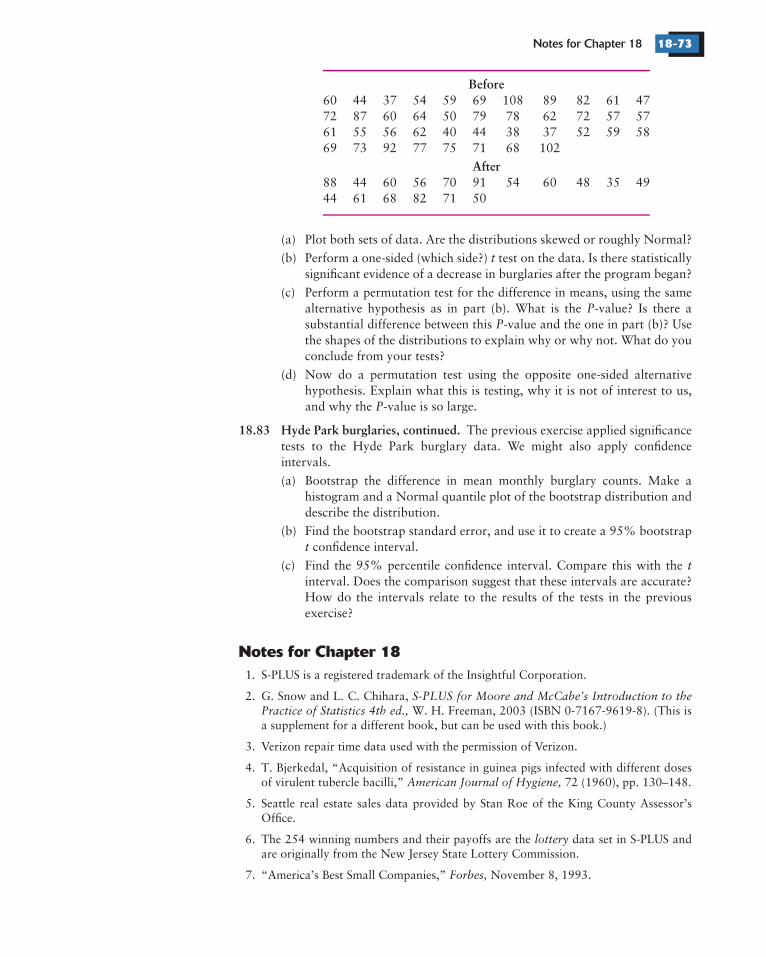
Notes for Chapter 18 18-73
Notes for Chapter 18
Before
After
18.83 Hyde Park burglaries, continued.
1. S-PLUS is a registered trademark of the Insightful Corporation.
2. G. Snow and L. C. Chihara,W. H. Freeman, 2003 (ISBN 0-7167-9619-8). (This is
a supplement for a different book, but can be used with this book.)
3. Verizon repair time data used with the permission of Verizon.
4. T. Bjerkedal, “Acquisition of resistance in guinea pigs infected with different dosesof virulent tubercle bacilli,” 72 (1960), pp. 130–148.
5. Seattle real estate sales data provided by Stan Roe of the King County Assessor’sOffice.
6. The 254 winning numbers and their payoffs are the data set in S-PLUS andare originally from the New Jersey State Lottery Commission.
7. “America’s Best Small Companies,” November 8, 1993.
S-PLUS for Moore and McCabe’s Introduction to thePractice of Statistics 4th ed.,
American Journal of Hygiene,
lottery
Forbes,
t
PP
P
t
t
60 44 37 54 59 69 108 89 82 61 4772 87 60 64 50 79 78 62 72 57 5761 55 56 62 40 44 38 37 52 59 5869 73 92 77 75 71 68 102
88 44 60 56 70 91 54 60 48 35 4944 61 68 82 71 50
(a) Plot both sets of data. Are the distributions skewed or roughly Normal?
(b) Perform a one-sided (which side?) test on the data. Is there statisticallysignificant evidence of a decrease in burglaries after the program began?
(c) Perform a permutation test for the difference in means, using the samealternative hypothesis as in part (b). What is the -value? Is there asubstantial difference between this -value and the one in part (b)? Usethe shapes of the distributions to explain why or why not. What do youconclude from your tests?
(d) Now do a permutation test using the opposite one-sided alternativehypothesis. Explain what this is testing, why it is not of interest to us,and why the -value is so large.
The previous exercise applied significancetests to the Hyde Park burglary data. We might also apply confidenceintervals.
(a) Bootstrap the difference in mean monthly burglary counts. Make ahistogram and a Normal quantile plot of the bootstrap distribution anddescribe the distribution.
(b) Find the bootstrap standard error, and use it to create a 95% bootstrapconfidence interval.
(c) Find the 95% percentile confidence interval. Compare this with theinterval. Does the comparison suggest that these intervals are accurate?How do the intervals relate to the results of the tests in the previousexercise?
Bootstrap Methods and Permutation Tests18-74 CHAPTER 18 �
www.forbes.com
www.espn.com
www.nasdaq.com
www.bls.gov
8. ACORN, “Banking on discrimination: executive summary,” October 1991, in
102nd Congress, 2nd Session, Serial 102-120, May 7 and May 14,1992, pp. 236–246.
9. From the Web site, .
10. Data provided by Darlene Gordon, Purdue University, for David S. Moore andGeorge P. McCabe, 4th ed., W. H. Freemanand Company, 2003.
11. From , July 2, 2002.
12. April 1990, pp. 235–288. These data are part of thedata set in S-PLUS.
13. Roseann M. Lyle et al., “Blood pressure and metabolic effects of calcium supple-mentation in normotensive white and black men,”
257 (1987), pp. 1772–1776.
14. Data from .
15. L. Friedland et al., “Effect of educational program on compliance with glove use in apediatric emergency department,” 146(1992), pp. 1355–1358.
16. From the Web site of the Bureau of Labor Statistics, .
17. F. K. Shuptrine and D. D. McVicker, “Readability levels of magazine ads,”21, No. 5 (1981), p. 47.
18. G. V. Glass, V. L. Wilson, and J. M. Gottman,Colorado Associated University Press, 1975.
JointHearings before the Committee on Banking, Finance, and Urban Affairs, House ofRepresentatives,
Forbes
Introduction to the Practice of Statistics,
Consumer Reports, fuel.frame
Journal of the American MedicalAssociation,
American Journal of Diseases of Childhood,
Journalof Advertising Research,
Design and Analysis of Time SeriesExperiments,