PRELIMINARY: Please do not cite or quote without permission · And, within air pollution, releases of carcinogens a re particu larly problema tic for infant health outcomes. We do

PRELIMINARY: Please do not cite or quote without permission

TOXIC EXPOSURE IN AMERICA:

ESTIMATING FETAL AND INFANT HEALTH OUTCOMES

Nikhil Agarwal*Chanont Banternghansa**

Linda T.M. Bui***

(July 2008)NBER Summer Institute

ABSTRACT: We examine the effect of exposure to toxic releases that are tracked by the ToxicRelease Inventory (TRI) on county-level infant and fetal mortality rates in the United States between1989-2002. We find significant adverse effects of TRI concentrations on infant mortality rates, butnot on fetal mortality rates. In particular, we estimate that the average county-level decrease inaggregate TRI concentrations saved in excess of 25,000 infant lives from 1989-2002. Using the lowend of the range for the value of a life that is typically used by the EPA of $1.8M, the savings in liveswould be valued at approximately $45B. We also find that the effect of toxic exposure on healthoutcomes varies across pollution media: air pollution has a larger impact on health outcomes thaneither water or land. And, within air pollution, releases of carcinogens are particularly problematicfor infant health outcomes. We do not, however, find any significant effect on health outcomes fromexposure to two criteria air pollutants – PM10 and ozone. ___________________* Harvard University, graduate student** Federal Reserve Bank, St. Louis*** Department of Economics, Brandeis University, 415 South Street, MS 021, Waltham, MA02454. Associate Professor, corresponding author. [email protected]

The authors would like to thank NCHS for providing the birth, death, and linked data files, and theNational Air Data Group of the EPA for the criteria air pollution data that was used in this paper.The authors gratefully acknowledge funding from the Norman Grant, Brandeis University, andwould like to thank Erich Muehlegger and T. S. Sims for helpful comments. All errors are our own.

cbeck

Typewritten Text

EEE 7/21/08 3:30 pm

1 See U.S. PIRG Report, executive summary (January 22, 2003).

2 No comprehensive data set exists for ambient toxic pollutants. Data on ambient toxicconcentrations for only a small number of toxic pollutants have been recorded for a select number of statesin 1996, and only periodically since that time.

-1-

TOXIC EXPOSURE IN AMERICA:

ESTIMATING FETAL AND INFANT HEALTH OUTCOMES

I. INTRODUCTION

Over 75,000 different chemical substances, used or manufactured in the United States, are

currently registered with the EPA under the Toxic Substances Control Act (TSCA). The majority

of these substances are relatively new, having been developed since World War II and, for many,

little is known about their effects on health. Since 1988, the Toxic Release Inventory (TRI) has

tracked environmental releases by manufacturing plants in the U.S. of 300-600 of these substances,

all of which are either known to be, or suspected of being, hazardous to human health. It is estimated

that, in 2000, more than 100 million pounds of carcinogens, 188 million pounds of developmental

or reproductive toxins, 1 billion pounds of suspected neurological toxicants, and 1.7 billion pounds

of suspected respiratory toxicants were released into the nation’s air, water, and land by the

manufacturing sector alone.1

Toxic substances in the U.S. face cradle-to-grave regulation: their storage, handling,

transportation, and disposal are all strictly regulated. Yet, for most of these substances, there is no

formal regulation of their releases into the environment. In part, this may be due to a belief that at

low levels of perceived exposure there are no significant health effects.2 And, to a large extent, there

was little public concern over toxic releases until the discovery in 1978 of toxic wastes buried

beneath a neighborhood in Love Canal, N.Y., and then of a strong correlation between residential

proximity to Love Canal and significantly elevated rates of cancer, neurological disorders, birth

defects, and still births.

Love Canal spurred a number of epidemiological studies into the health effects of toxic

exposure. The bulk of that research consists of cross-sectional studies, usually on adults, and

provides mixed results on the relationship between toxic pollution exposure and health outcomes.

-2-

That is similar to what has been observed in the literature on (non-toxic) air pollution and health.

As pointed out by Greenstone and Chay (2003a), the lack of consensus on the effects of air pollution

on health may be explained by serious problems in identification in cross-sectional studies due to

omitted variable bias. Furthermore, studies of adult health outcomes may be flawed by the inability

to measure accurately life-time exposure to pollutants. Even abstracting from mobility issues, using

current levels of pollution to proxy for life-time exposure will be inaccurate if pollution concentrat-

ion levels have changed dramatically over time, as is true of toxic pollutants (Needham et al. (2005)).

In this study, we focus on the health effects from toxic pollution exposure on two particularly

vulnerable groups: fetuses surviving at least 20 weeks in utero and infants under one year of age.

By doing so, we mostly avoid the problems associated with trying to proxy for life-time exposure

levels. Empirical studies have shown that mobility rates for pregnant women are low, so that fetal

exposure reasonably can be approximated by pollution concentrations at the mother’s county of

residence.

We construct a panel data set that makes use of facility level annual toxic release data that

we aggregate to the county-year level, and link to files of all births and deaths in the U.S. between

1989-2002. We include covariates to control for a number of potentially confounding effects. Our

central identification strategy is based on exploiting the high level of variation in TRI concentrations

both between counties and within counties over time.

Our preliminary findings suggest that there are significant health consequences to infants of

exposure to toxic releases, although we do not find similar outcomes for fetal health. In particular,

we estimate that the over-all change (decrease) in annual average county-level TRI concentration (net

of pollutants regulated under the Clean Air Act (CAA)) that occurred between 1989-2002 was

responsible for a decline of over 25,000 infant deaths. Valued at between $1.8M - $8.7M per life,

this savings would be valued at between $45B - $217.5B.

We also find that the medium by which the toxic pollutants are released into the environment

matters for health outcomes: toxic air releases are significantly more harmful to infant health than

either water or land releases. This may suggest something about the mechanism by which infants

are exposed differentially to these substances. We find also that carcinogenic air releases have the

largest effect on infant mortality of all the pollutants that we study. In contrast to other studies, we

-3-

do not, however, find any measurable health effects on infants from exposure to ambient

concentrations of either particulate matter (PM10), or ozone (O3).

The rest of the paper is organized as follows. In section II we provide a brief summary of the

literature, focusing in particular on epidemiological studies that relate fetal and infant health

outcomes to toxic pollution exposure. We discuss data sources that are used in our study in section

III; descriptive statistics are given in section IV. Section V describes our methodology and section

VI discusses data issues. In Section VII, we present our preliminary results. In Section VIII we

provide describe tests for robustness that we conduct on the data, and in Section IX, we discuss

policy implications and provide concluding remarks.

II. BACKGROUND

It is generally believed that both fetuses and infants are particularly vulnerable to exposure

to toxic pollutants, although the biological mechanisms through which they occur are not yet well

understood. The National Research Council described four ways by which these two groups were

uniquely vulnerable to environmental toxins (Landrigan et al. (2004)). First, children have

disproportionately heavy exposures to many environmental agents because of their size. Relative

to their body weight, they consume significantly more food and water than adults. Toxins that are

present in the food system or in the water supply may therefore be more harmful to them than to

adults. Second, because the central nervous system is not fully developed until at least 6 months post

birth (Choi (2006)), the blood-brain barrier may be breached by certain environmental toxins, in a

manner that is less likely later in life. Third, developmental processes are more easily disrupted

during periods of rapid growth and development before and after birth, making exposure to

environmental toxins during these stages particularly harmful. And fourth, because children have

longer life-spans, exposure to environmental toxins at an earlier age, or even in utero, may lead to

a higher probability of developing a chronic disease that might not occur if exposure were to occur

later in life.

Before addressing the question of fetal or infant health outcomes from exposure to

environmental toxins, it is important to address directly the question of how to measure toxic

exposures. Fetal exposure is a direct consequence of maternal exposure. Most studies assume that

-4-

the relevant level of exposure may be captured by the mother’s place of residence at the time of

delivery. That will only be true, however, if the mobility rate of pregnant women is low. Published

studies have estimated residential mobility during pregnancy to range between 12% - 32%, with one

study estimating that, of those that moved, only 5% changed municipality and 4% changed county

during pregnancy. (See Fel et al. (2004), Khoury et al. (1988), Shaw et al. (1992), and Zender et al.

(2001).) In combination, those studies would suggest that, at most, 1% of pregnant women would

not have been in residence within the birth-designated county during their pregnancy. Fel et al.

(2004) also report that, in their study, mobility was not correlated with exposure to chemicals or

pesticides in the workplace or at home. They did find, however, that both younger (age < 25) and

older (age >35) women were more mobile, as were unemployed women and those from lower

income groups.

Several epidemiological studies look at health outcomes for prenatal exposure to toxic

pollutants. A number of papers find a correlation between prenatal exposure and spontaneous

abortion, malformation, and low birth weight (Bove et al. (1995), Carpenter (1994), Landrigan et al

(1999)). Others, however, find no such correlation (Baker et al (1988), Croen et al (1997), Fielder

et al (2000), Kharrazi (1997), Sonsiak (1994)). More recent work suggests that the health effects

may be tied only to particular categories of toxic pollutants. For example, Meuller et al. (2007) look

at the relationship between fetal deaths and maternal proximity to a hazardous waste sites, but finds

statistically significant results only for proximity to waste sites associated with pesticides.

Infant health outcomes may be affected both by exposure that occurs in utero and after birth.

It is well documented that infants are at particular risk for exposure to heavy metals, such as lead and

methyl mercury (Landrigan et al. (2004 )). Choi et al. (2004) find that there is a higher risk of

developing childhood brain cancers when mothers live close to a TRI emitting facility. Making use

of TRI data, Marshall et. al (1997) find that there is a slight increase in certain birth defects due to

exposure to toxic releases.

Because of similarities in terms both of econometric issues and issues of causality, it is useful

to look also at the literature on air pollution and health. Greenstone and Chay (2003a), for example,

examine the effects of total suspended particulates (TSPs) on infant mortality rates. They use the

changes in TSP pollution concentrations that were generated by the 1981-82 recession as a “quasi-

-5-

experiment” to identify changes in infant mortality at the county level in the U.S. Their underlying

assumption is that the recession-induced variation in county-level TSP concentrations is exogenous

to infant mortality rates. They compare cross-sectional results for each year between 1978-1984 to

a panel-data, fixed effects model (in first-differences) and show that the traditional cross-sectional

approach can produce misleading results due to unobserved, omitted confounders. Using an

approach that mitigates many of these identification problems, Greenstone and Chay find that a 1

:g/m3 reduction in TSP concentration results in approximately 4-8 fewer infant deaths per 100,000

live births at the county level. Over the 1980-82 recession, they estimate that the reduction in TSPs

led to approximately 2500 fewer infant deaths.

Currie and Neidell (2005) also look at the relationship between ambient air pollution

concentrations and infant and fetal mortality. They focus on California during the 1990s and

examine 3 different criteria air pollutants: carbon monoxide, particulate matter, and ozone. Unlike

most other air pollution studies, Currie and Neidell allow for correlations across pollutants in their

effect on infant mortality. Taking individual data that they aggregate up to the zip code-month level,

they estimate an approximate linear hazard model and find a significant effect of carbon monoxide

on infant mortality (although not on fetal mortality) and estimate that the significant reduction in

carbon monoxide concentrations in California saved approximately 1,000 infant lives over the 1990s.

Taking our cues from both Greenstone and Chay (2003a, 2003b) and Currie and Neidell

(2005), we make use of the variation in TRI releases across location (by county) and time to identify

the effects of TRI releases on health outcomes. To control for potential confounding effects, we

include parental characteristics, prenatal care information, and medicaid and other income transfers.

We also allow for the possibility that other types of pollution exposure may affect health outcomes.

In particular, we include measures for particulate matter and ozone concentration. Those two criteria

air pollutants may also proxy for toxic air pollution concentrations that derive from mobile sources

of pollution, as they are highly correlated with fuel combustion.

III. DATA

We combine data from various sources to construct a comprehensive set of measures at the

county level for the period 1989-2002. Data on pregnancy outcomes are from the National Center

3 An infant is defined as being an individual under one year of age.

-6-

for Health Statistics (NCHS). Data on toxic emissions are from the Toxic Release Inventory,

maintained by the U. S. Environmental Protection Agency (EPA). Those two data sets are

supplemented by county level data on income, job composition, transfer payments from health and

unemployment benefit programs, and population, all from the U.S. Bureau of Economic Analysis.

Data on land and water area are taken from the U.S. Census 2000 Gazatteer Files. In this section we

provide a detailed description of the primary data used in this study.

Health Outcomes Data

Our dependent variable and many important control variables are taken from infant3 birth and

death records, and fetal death records provided by NCHS. These records are constructed from a

census of death and birth certificates, as required by law in all states.

The NCHS, in cooperation with the states and territories of the U.S., has promulgated a

uniform instrument with which to collect information on each fetal death. (Note that our estimate

of pregnancies comes from adding births and fetal deaths in a given year, as such it does not include

terminated pregnancies.)

Infant Data: Birth certificates contain information about the parents of the baby, in

addition to limited details about the medical history of the mother and the specific pregnancy. The

variables that we use as controls include the reported age, education, marital status and race of the

parents; tobacco and alcohol consumption; and the level of pre-natal care as indicated by the number

of prenatal visits to a doctor.

We use death certificates to identify the cause of death as coded using the International

Classification of Diseases. We remove infant deaths caused by external factors such as physical

injuries from our measures, as they should not be related to the exposure of toxic releases. We refer

to the retained observations as “internal” infant deaths.

It should be noted that death records generally do not contain information on county of

maternal residence. We therefore compute the internal infant death rate as the ratio of infant deaths

in a county to births by mothers residing in a county.

Fetal Data: Information in the fetal death files includes some of the same

-7-

information that is available in birth certificates, such as the reported age, education, marital status

and race of the parents; tobacco and alcohol consumption; and the level of prenatal care. The period

of gestation is also included. Deaths of fetuses at less than 20 weeks are not well reported in the data

set. Birth certificates and fetal death records also report the county of the mother’s residence coded

using the Federal Information Processing Standard (FIPS).

Using the individual level data described above, we compute county level statistics based on

the county of residence of the mother, for infant death rates due to internal causes, and death rates

for fetuses with a period of gestation of more than 20 weeks. Our control variables are also

aggregated to the county level, by computing averages of measures such as maternal and paternal

age, maternal years of education, and the number of prenatal visits. We also compute for each

county and year the fraction of pregnant mothers in each of the following categories: white, African-

American, smoking mothers, mothers that consume alcohol, and mothers that are married. The

health data set, thus aggregated to the county-year level by the residence of the mother, is then

merged with a data set on toxic releases.

Toxic Release Data

Data on toxic releases are taken from the Toxic Release Inventory. The TRI was introduced

in 1986 under the Emergency Planning, Community Right To Know Act (EPCRA) and requires that

all manufacturing plants with ten or more full time employees that either use or manufacture more

than a threshold level of a listed substance report their toxic releases to a publicly maintained

database. The first year of reporting was in 1987. At that time, there were approximately 300 TRI

listed substances. In 1995, this list was expanded to include 286 new substances. Today (2008), the

TRI covers 581 individually listed chemicals, 27 chemical categories, and 3 delimited categories

containing another 58 chemicals. Reporting thresholds have remained at 10,000 lbs (annually) for

most chemicals, with the exception of 4 persistent, bio-accumulative, toxic chemical (PBT)

categories, and 16 PBT chemicals. ( EPA website: www.epa.gov/tri/lawsandregs/pbt/pbtrule.htm)

Because of changing thresholds and both the addition and deletion of reporting chemicals over time,

we restrict our analysis to the stable base set of 1988 chemicals that are not affected by changing

reporting thresholds.

TRI data are reported at the facility level. Separate reports are filed for each TRI substance

-8-

for which the facility meets the reporting requirements. Data are broken down by medium (air,

water, underground, etc.), and information is provided as to whether the substance is known to be

carcinogenic. Using TRI-provided information on chemical CAS number, we further classify TRI

chemicals as a developmental or reproductive toxin if it is listed as such in the State of California

Safe Drinking Water and Toxic Enforcement Act. The TRI data set also provides information on

whether a given chemical is simultaneously regulated under the Clean Air Act.

Using this, we construct, for each county-year observation, the total pounds of TRI releases

net of any Clean Air Act releases by air, water, and “land” (where land is the residual category =

aggregate releases - air releases - water releases); broken down into by carcinogenic, and

developmental and/or reproductive emissions. (We exclude CAA chemicals from our measures of

TRI concentrations to avoid any possibility of “double counting” because we include measures of

criteria air pollution concentrations in our models of health outcomes.) Using geographic data from

the Census 2000 Gazatteer Files, we construct a crude measure of “concentration” by dividing total

pounds of releases by land-area.

Criteria Air Pollution Data

When examining the relationship between TRI releases and health, it is important to control

for the effect that other pollutants may have on health outcomes. We therefore supplement the TRI

pollution data with data on concentrations of criteria air pollution, as provided by EPA’s National

Air Data Group. Those data were extracted from recordings taken from pollution monitors located

in various counties across the nation. The data set provides means, variances, medians, and higher

percentiles of concentrations observed by monitoring stations in a given day of a year. Of these

values, we make use of the daily average concentration and the 95th percentile concentration. In

some counties, there are multiple monitoring stations. In those cases, we use the simple average

across all monitoring stations for the daily average concentration and for the 95th percentile

concentration. Most counties, however, do not have any monitoring stations that measure all

categories of criteria air pollution concentrations. We choose to concentrate on particulate matter

(PM10 ) and ozone (O3) because these pollutants had the least number of missing county level

observations, and because a number of studies have shown a potential link between their ambient

concentration levels and adverse health outcomes for both infants and the unborn. An additional

4 Further discussion of how these observations were chosen, and the robustness of findings basedon the restricted sample, is found in Section VI.

-9-

benefit of including PM10 and O3 in our study is that they are highly correlated with mobile source

emissions of pollution. This is important, as we cannot directly control for mobile sources of

pollution, and they are known to be major contributors to airborne toxic releases.

Other Data Sources

Several county level controls are also used in our study. Data on per capita income,

Medicaid transfers, food stamp participation, and other government supplemental income transfers

are taken from the Bureau of Economic Analysis (BEA). The fraction of the labor force employed

in the manufacturing sector as well as county-level unemployment rates also come from the BEA.

IV. BIRTHS, DEATHS, AND TOXIC RELEASES: 1989-2002

The TRI-internal infant death and fetal death data set, linked with county-level demographics

data, consists of 42,370 county-year observations. Between 1989-2002, there were over 56 million

live births in the United States, with just under 420,000 internal infant deaths and 889,000 fetal

deaths recorded. More than 55.8 billion lbs of toxic pollutants were released into the environment

from the manufacturing sector, 4.2 billion lbs of which were carcinogens (2.9 billion lbs in the form

of air releases), and 3.9 billion lbs of which were developmental or reproductive toxins (27.7 million

lbs in the form of air releases).

Of the 42,370 county-year observations for which we have TRI, birth and infant/fetal death

information, and county-level demographic information, only 11%, or 4,528 county-years, also have

air monitoring stations that collect PM10 and ozone concentrations. The restricted sample that

includes observations on (non-toxic) ambient air pollution concentrations captures 32.5 million live

births, or 58% of the total, over the sample period, and is the basis for the regression analysis.4

Select summary statistics for this more restricted data set (the “regression” sample) are presented in

Tables 1-3, and described below. It consists of an unbalanced panel with between 243-350 counties

in the United States. Those counties range in population from as small as 2,300 to as large as

9,700,000.

In real terms, average per capita income level is increasing during our sample period, as are

5 See, for example, the meta-analysis done by Fade, Vivian B, Graubard, Barry; “AlcoholConsumption during Pregnancy and Infant Birth-Weight,” Annals of Epidemiology. 4,4 (July 1994):279-284.

-10-

medicaid transfers (as well as other income transfers). Not surprisingly, the percentage of jobs in

the manufacturing sector steadily declined. That may be important for our study, as TRI releases

come predominantly from manufacturing, and workers in that sector may experience additional

exposure to toxic chemicals in their workplace, which may in turn affect infant and fetal health

outcomes.

With respect to parental characteristics that may affect health outcomes, we note that the

average maternal age at birth increased slightly over time. If due to a reduction in teenage

pregnancies, which are known to be associated with poorer health outcomes for both the fetuses and

infants (reference), this might lead to lower infant and fetal mortality rates. If, on the other hand, it

is due to women bearing children later in life, it might be detrimental to fetal and infant mortality.

Maternal behavioral characteristics, however, clearly point to potential improvements in fetal and

infant health. The consumption of tobacco during pregnancy fell dramatically over the 14 years

covered by our study, from a high of 16.44% to a low of 8.61%. The consumption of alcohol during

pregnancy likewise fell between 1990-1999, but then rose dramatically. One possible explanation

for that reversal is an increasing number of studies began to suggest that there were positive (or no)

health effects, for both mother and fetus, of a very small amount of alcohol consumption during

pregnancy.5

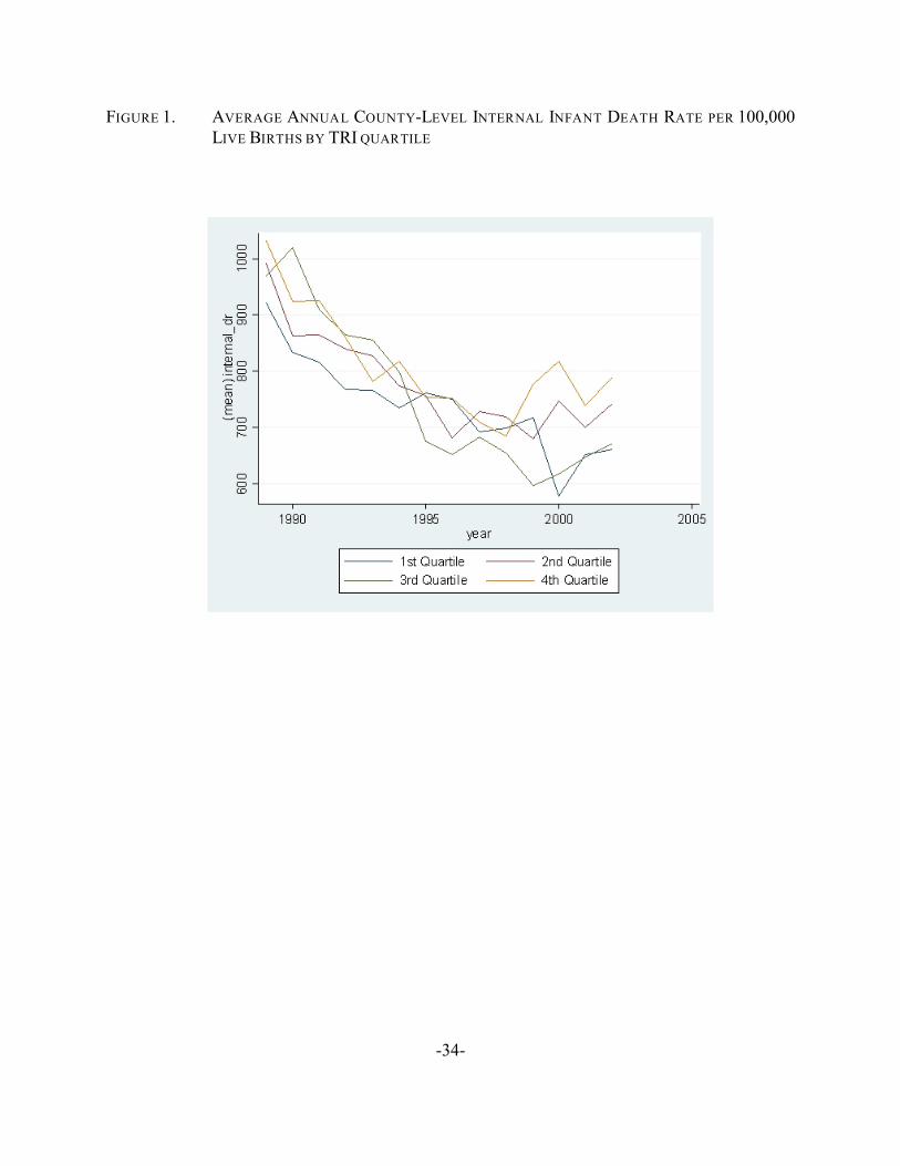
Nationwide, mean county-level infant deaths from internal causes declined almost

monotonically between 1989-2002 from 948.9 to 660.9 deaths per 100,000 live births, or by nearly

30%. A smaller decline (9%) was observed for fetal deaths (post 20 weeks gestation). In our

regression sample, we observe a similar decline for infant deaths from internal causes (approximately

28%), but a much larger decline in fetal deaths (33%) than the national trend. We note also that

internal infant mortality rates vary significantly across TRI concentrations (net of Clean Air Act

chemicals) by quartile, being significantly higher for the dirtiest TRI counties. The same pattern

holds true for fetal mortality rates. (See Figures1and 2.)

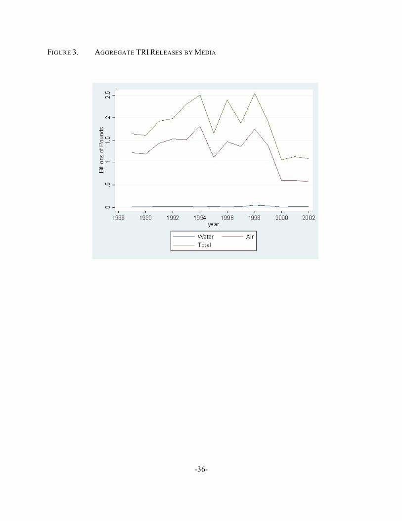
Although TRI releases have fallen significantly when compared to their originally reported

6 See, for example, Greenstone and Chay (2003a).

-11-

levels in 1988 (over 40%, nationwide), the decline in releases has been far from monotonic. In our

regression sample, between 1990-1999, aggregate TRI concentrations rose by over 140%.

After1999, they fell by more than 65%. Similarly, TRI air concentrations increased by 22% between

1990-1999 and fell by 53% between 1999-2002. The pattern for carcinogenic air concentrations is

likewise, volatile. Carcinogenic air concentrations more than doubled between 1996-1997, and then

increased by more than 16-fold between 1998-1999. It then fell by more than 85% between 1999-

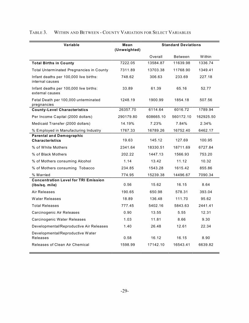
2002. (Similar patterns exist for the unrestricted sample of TRI reporters.) A quick glance at Table

3 shows that the variation in TRI releases, in aggregate form, as well as by select categories, is high

both within and between counties.

In contrast to TRI concentrations, ambient air concentrations for ozone and particulate matter

are quite stable throughout our sample. Average county-level ozone concentrations (ppm) rose from

0.0248 to 0.0283, whereas PM10 concentrations (:g/m3) fell from 33.28 to 25.24. The variance in

concentrations is very small, across time, across county, and even within county.

V. METHODOLOGY

To estimate the effects of toxic pollution on health outcomes (infant and fetal mortality), we

adopt the widely used approach of assuming that the effects of the covariates on health is linear and

additive.6 The “true” model can thus be described by:

(1)

(2)

where, i indexes county and t indexes year. Xit is our independent variable of interest, the

concentrations of TRI releases; Zit are a set of covariates that capture aggregate parental

characteristics; Wit are controls for county-level income distribution and non-toxic air pollution

concentrations, and uit is an orthogonal error term.

To estimate $ consistently, we require E[Xit@ ,it] = 0. By omitting county-fixed or time-fixed

factors such as "i or (t that are correlated with both TRI concentrations and infant (fetal) health

-12-

statistics, we may introduce bias into the estimate of $. Unobservables that vary by county and year,

like 8it, may also bias the estimates if they are correlated with Xit. Ideally, one would like to

introduce county-time interaction effects to absorb all potential sources of bias. That is not,

however, feasible, due to a constraint on our degrees of freedom.

To efficiently estimate (1), we can use a first-difference model to remove the county-level,

unobserved fixed effects. To do so, we take the difference between county level observations at

period t and t-1 to obtain:

(3)

(4)

For consistent estimation of (3) after including time-fixed effects to control for )(t, we need

to assume that E[)Xit@)8it] = 0. This would imply that the change in pollution concentration

undertaken by manufacturing plants in a particular county is not correlated with changes in other

(uncontrolled) factors that are correlated with levels of pollution in that county. To control for any

potential sources of bias that might violate E[)Xit@)8it] = 0, we include state-time (in lieu of county-

time) variables in our first-difference model. Our ideal equation for estimation using generalized

least squares, weighted by the number of live births in a county (or number of unterminated

pregnancies, in the case of fetal deaths), is then:

(5)

where s indexes the state of county i.

For consistent estimation of (5), we must assume that E[)Xit@ <it] = 0. Intuitively, we are

saying that the distribution of toxic pollution from the manufacturing sector across counties within

a given state is exogenous to variations in county characteristics that may affect infant (fetal)

mortality rates and that are not captured in )Zit or )Wit. Since we control for state-time interaction

effects, we need only assume that the location choice of different types of manufacturing industries

(heavy polluters or otherwise) within a state is random with respect to other factors that might affect

pre-natal or peri-natal health. Our assumption will also be reasonable as long as the variation in )8it

-13-

within a state is low for each year in our sample. Our maintained assumption is that, by controlling

for state-time interaction effects we have eliminated most sources of potential bias from our model.

An examination of the correlation between the TRI release statistics and covariates, Zit and

Wit indicate that the correlation between the levels of TRI pollution and most parental and county

characteristics is low, as well as with the criteria air pollution concentrations (see Table 2). Only for

Medicaid benefits do we observe a correlation greater than 15% with pollution concentrations. (For

the sample of large counties > 250,000 in population, post 1996, we also find high correlations

between pollution measures and demographic characteristics like racial composition and percentage

of children born in wedlock. This, in and of itself, may be important for issues relating to

environmental justice and public policy.) In any event, the correlation measures for those variables

that we can explicitly control for suggests that bias due to 8it should not be large. It may also be

argued that if enough factors that potentially affect pre-natal and peri-natal health are controlled for,

we do not need to worry about bias from )8it because our existing controls will absorb the effect of

such confounding variables. A Hausman test for exogeneity may be used to test that hypothesis

directly.

VI: DATA ISSUES

Although our full data set consists of approximately 42,370 county-year observations, we

have relatively few observations for county-level criteria air pollution concentrations, reducing the

total number of county-year observations available for our regression analysis to 4,198. When

estimating the model described by equation (5), we also eliminate a small number of outliers, so that

the estimating data set consists of 4,154 observations. We define outliers as being observations for

which the change in total TRI concentrations (net of CAA chemicals) are either in the top or bottom

0.5% of the over-all distribution (based on the 42,370 county-year observations). For the regression

data set, this amounts to dropping the top 23 and bottom 21 observations for changes in aggregate

TRI concentrations. This restricted data set captures approximately 54% of all live births in the U.S.

over our sample period.

We also find that a large number of counties report no TRI releases in a given year. This may

be because there was no manufacturing activity in that county, or none of the facilities met the

7 The mean, annual, county-level concentration of aggregate TRI pollution (X&) is 675.7 lbs/sq. mile.The mean, annual, county-level number of internal deaths (Y &) is 775.6. Using these numbers, we can

-14-

reporting criteria. In the case where there was no manufacturing activity, then the correct measure

for TRI releases in that county would be zero. If, however, the facilities simply did not meet the

reporting requirements – due to the size of the facility, or by falling below the reporting threshold,

a “zero” level of TRI release would under-estimate the true value. For our purposes, we report

“zero” levels of releases for all non-reporting counties. This will tend to under-estimate the effects

of TRI releases on health outcomes.

All results and estimates of elasticities, and numbers of lives lost or saved are based on the

restricted regression sample which excludes outliers.

VII. PRELIMINARY RESULTS

Table 4 summarizes the effects of TRI concentrations on infant mortality and fetal mortality

(post 20 weeks) rates per 100,000 live births or 100,000 unterminated pregnancies from estimating

the first-difference model described in (5), above. All models include year dummies and year-state

interactions. The infant mortality regressions are weighted by total number of live births in each

county and year, whereas the fetal mortality regressions are weighted by the total number of

unterminated pregnancies. Robust standard errors that allow for correlation across states are

reported. Controls for parental characteristics are included in each specification as well as measures

for real per capita income and medicaid transfers. We also include air pollution concentrations for

PM10 and ozone that are recorded at air monitoring stations across the country. Hausman tests were

used to test the exogeneity assumption required for (5) to yield consistent estimators, and in each

specification described below, the null hypothesis of exogeneity could not be rejected at a 5% level

of significance.

Aggregate TRI Releases

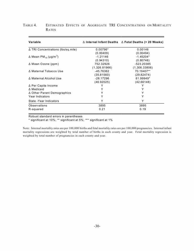
The estimated coefficient on aggregate TRI concentrations in the infant mortality regression

is 0.008 and is statistically significant at the 5% level. This yields an implied elasticity of infant

mortality with respect to TRI-concentration measured at the mean of approximately 0.007.7 Using

calculate the elasticity as: or, 0.008 (675.7/775.6) = 0.007. See Table 7 for all values used in

the elasticity calculation and the confidence interval on lives lost or saved.

-15-

the annual, county-level average change in aggregate TRI concentration of -1.2%, or approximately

8.1 lbs/sq.mile/year, we estimate that over the 14 year sample period, the decrease in TRI

concentration led to a savings of 25,237 infant lives. Using values of life numbers commonly used

by EPA ($1.8M - $8.7M per life) suggests an aggregate value for these lives of $45.4B - $219.6B

(see Table 7). We do not find any relationship between aggregate TRI concentrations and fetal death

rates, post 20-weeks of gestation.

Somewhat surprisingly, we do not find any effects of non-toxic air pollution concentrations

on health outcomes for infants. Those findings are robust to using either the mean aggregate

concentration level or the 95th percentile measure for ozone and PM10. One possible explanation

may be that average county-level concentration levels are quite low during our sample period so that

the health effects are small. Also, there is little variation across counties or over time in ambient

ozone or PM10 concentrations in our data, which could explain the large standard errors on these two

coefficients.

We do, however, observe that ambient concentrations of mean county-level particulate matter

have a statistically significant, negative effect on fetal mortality rates. That is, when particulate

matter concentrations increase, fetal death rates observed in the sample fall. Although this may be

counter-intuitive, what it may reflect is a “harvesting” effect. Our data are limited to fetal deaths

after 20 weeks gestation, and the fall in deaths among that group may be due to an increase in pre-20

week fetal deaths. Unfortunately, we cannot reliably test this hypothesis, because of the poor data

quality on pre-20 week fetal death data.

Consistent with findings in other pollution-health studies, we find that per capita income and

medicaid payments do not affect infant or fetal health outcomes. Maternal behavior, however, has

a measurable effect on fetal mortality rates. There is a strong, positive correlation between tobacco

and (despite some then contemporaneous studies suggesting the contrary) alcohol use and fetal

mortality rates: increased use of either significantly increases the rate of fetal mortality post-20

weeks gestation.

-16-

TRI by Air and Water and Land

One question of interest is whether different pollution media have differential effects on

health. For example, infants undergo direct exposure to air pollution and their small and less

developed lung capacity may adversely affect their ability to deal with airborne toxins. They may

thus be more susceptible to air than water pollution. Fetuses, on the other hand, are exposed to both

air and water pollution only through maternal exposure. The mechanisms through which maternal

exposure lead to fetal exposure almost surely differ across pollution media.

In Table 5, we report estimates for TRI concentrations partitioned by air, water, and “land,”

where land is simply the residual level of release once air and water releases are accounted for. We

find that neither TRI water nor land releases have a measurable effect on either infant or fetal

mortality rates. TRI air releases, however, have a large, significant effect on infant mortality rates.

The coefficient on TRI air concentration is 0.023, implying an elasticity of approximately 0.005. For

an annual average change in TRI county-level air concentration of -4.86% for 14 years, this would

imply a savings of 73,776 infant lives, or $132.8B -$641.85B (see Table 7).

In the partitioned regressions we again find no statistically significant effects of non-toxic

air pollution concentrations, per capita income levels, or income transfers on infant mortality rates,

but we do still observe the (potential harvesting) effect of particulate matter on fetal mortality (post

20 weeks gestation). The effects of maternal behavior (tobacco and alcohol use) on fetal mortality

rates are also similar to those found in the regressions using aggregate TRI concentrations.

TRI Carcinogens, Developmental, and Reproductive Toxins

Exposures to carcinogens and to developmental or reproductive toxins, are thought to be

particularly hazardous to human health. Here, we look to see whether toxic releases that are either

known or are suspected carcinogens, or developmental/reproductive toxins have a measurable affect

infant and fetal mortality rates.

Because of our earlier finding that different pollution media may have different health effects,

we now parse aggregate TRI releases (net of CAA pollutants) by both media (air, water, and land)

and type (carcinogenic, developmental/reproductive, “other”), including a separate variable for each

of the 9 different categories. We summarize our results in Table 6. What we find is that carcinogenic

air concentrations have a large, significant adverse effect on infant mortality. With a coefficient

8 In the regression used to conduct the Hausman test, which included both levels and first-differences of the independent variables of interest, no levels variables were found to be individuallystatistically significant except for that on the developmental or reproductive water concentrations variable,which had a t-statistic greater than 2.

-17-

estimate of 0.33, or an implied elasticity of 0.0005, this suggests that given an average, annual,

county-level increase in carcinogenic air concentrations of 0.8%, 1264 infant lives were lost between

1989-2002, with a value of between $2.28B - $11B. (See Table 7.)

We also find, however, that developmental/reproductive water concentrations have a large,

beneficial effect on infant mortality. With a coefficient estimate of -0.66, and an implied elasticity

of -0.0002, we estimate that the decrease in developmental/reproductive water concentrations of

6.9% (average, county-level increase), this led to a loss of 3666 lives between 1989-2002. One

possible explanation for this surprising result on TRI developmental/reproductive water

concentrations is that there may be a harvesting effect. Although we do not see any effect of

developmental/reproductive water concentrations on fetal deaths post 20 weeks gestation (we

observe a negative, non-significant effect), with respect to fetal deaths pre-20 weeks gestation, we

do find a negative, significant effect (with the understanding that the data are not very accurate). A

conceivable explanation may be that higher exposure to developmental or reproductive toxins leads

to an increase in terminated pregnancies of potentially less-viable fetuses, which in turn may lead

to a decline in fetal and infant death rates. Data on pregnancy terminations, unfortunately, is difficult

to obtain. Further investigation on the validity of this result is still necessary.

It is important to note, however, that although this particular specification does not actually

fail to reject the Hausman test for exogeneity, the p-value on the test (8%) is actually close to

rejecting exogeneity at conventional levels, and it is the developmental/reproductive water

concentration variable that appears to drive this result.8 That raises concerns for the possibility that

at least some of the coefficient estimators are biased and inconsistent in this model. And as just

noted, we have reason to be concerned about the developmental/reproductive water concentration

variable. This is not an issue in the aggregated models of TRI concentrations (presented in Tables

4 and 5), as this variable makes up a small proportion of over-all TRI releases (under 0.04%, on

average, in any county-year). For our less-aggregated model, however, it is important to ensure that

the values of the other estimated coefficients are robust. To do so, we re-estimate that specification,

-18-

excluding the TRI developmental/water concentration variable. Reassuringly, we find that all

coefficient estimates remain robust. Furthermore, in this restricted model, the p-value on the

Hausman test rises to p = 0.86 (consistent with the p-values found in the aggregated TRI models),

indicating that the coefficients have been consistently estimated.

We find a similar, negative effect with respect to developmental/reproductive air

concentrations on fetal mortality. The coefficient estimate is -0.22, yielding an implied elasticity

between fetal mortality and TRI developmental/reproductive air concentrations of -0.0004. With an

average, annual, county-level decline of 2.62%, this would lead to an increase, over 14 years, of

approximately 2865 additional fetal deaths.

VIII. ADDITIONAL CHECKS FOR ROBUSTNESS

Because of the complicated nature of our data set, it is important to ensure that our

regression results are not driven by spurious correlation, outliers, or sample selection. Here, we

discuss some of the tests for robustness that we conducted.

The most significant loss of data was due to the small number of county-year observations

for which we have PM10 and ozone concentration data. Although we believe that it is critical to

include these measures because (1) they may affect infant and fetal mortality rates and (2) they proxy

for toxic releases from non-manufacturing sources (e.g. mobile sources of pollution), we re-

estimated all regressions excluding those variables. In doing so, the total number of county-year

observations that may be included in the regressions increases to 38,277, once the top and bottom

0.5% of the change in aggregate TRI county-year concentration observations are trimmed as outliers.

(The number of observations reported here is more than 1% smaller than the full TRI-infant/fetal

health data set due to the loss of county-year observations for which we do not have data on per

capita income or other income transfers.) Not surprisingly, we find that using the larger sample

(excluding PM10 and ozone concentrations) the coefficient estimates (standard errors) on the

variables of interest are somewhat smaller (bigger) than for the restricted models reported in Tables

4-6, but of the same sign, magnitude, and general significance level. This shows both that the

omitted variable bias is small (recall from Table 3 that the correlations between the criteria air

pollution concentrations and TRI concentrations are less than 10%), but exists; and also that the

-19-

sample of counties for which we have air monitoring data does not introduce any significant sample

selection bias.

We also explore the sensitivity of our results to our having assigned a “zero” concentration

levels to counties that do not report TRI releases. That procedure tends to underestimate the health

effects of TRI concentrations. To verify that this is the case and to obtain an upper bound on the

health effects, we re-estimate all models excluding any county-year that has “zero” aggregate TRI

concentration. The estimated coefficients remain stable (and, as anticipated, they are somewhat

larger), and the level of statistical significance does not change dramatically. Hence, we conclude

that little bias is introduced by that procedure.

There are also concerns with the accuracy of TRI reported releases in the early years of

reporting, as well as with the quality of the infant birth and death files for small counties. As a check

on these potential problems, we make use of the linked birth-death records for infants that exist for

the years 1996-2001. The linked birth-death files exclude all births and deaths that cannot be linked

due to low data quality. On average in a given year, over 95% of all infant death records are linked

with the corresponding birth certificate. The public use linked files contain information on infant

births and deaths for all counties with populations greater than 250,000. This data set consists of a

balanced panel of 199 counties, accounting for approximately 58% of all live births in the country

(8.12 million births of 14 million, nationwide, from 1996-2001). Using this much smaller and more

restricted data set, our basic regression results remain robust.

Finally, as previously noted, we exclude a small number of outliers from our regression

analysis. Outliers are defined as being in the top or bottom 0.5% (approximately) of the distribution

for annual average county-level changes in TRI concentrations. In total, approximately 1% of our

county-year observations were excluded, of which over 57.55% reported no TRI releases.

Robustness checks on the stability of our results over different outlier criteria were conducted and

all results are robust over all specifications.

IX. CONCLUSION

Although the transportation, storage, handling, and disposal of toxic substances are regulated,

in general, their releases into the environment are not. Yet, the potential health effects from

-20-

exposure to these toxins could be devastating. Here, we attempt to look at the health effects from

exposure to a large body of these chemical substances on two of the most vulnerable groups in

society – infants and the unborn. The primary question of concern is whether at the current levels

of toxic releases and their corresponding levels of toxic concentrations there are measurable adverse

health consequences. A preliminary analysis of the data suggest that there are potentially large,

statistically significant effects on infant mortality rates with increases in toxic concentrations. We

find that infants are more sensitive to airborne concentrations of toxins than either land or water-born

concentrations, over-all, and that they are particularly vulnerable to carcinogens. Between 1989-

2002, we estimate that while the decline in average annual county-level TRI concentrations saved

over 25,000 infant lives, an estimated gain of $45B-$217.5B.

From a policy perspective, our findings suggests that if government programs were to be

developed to encourage reductions in toxic releases, the biggest health benefits for infants would

come from policies aimed at reducing toxic air releases, in general, and carcinogens, in particular.

Our research also highlights the need for monitoring of toxic pollution concentrations across

pollution media. Currently, no comprehensive tracking exists. Our results are based on very crude

measures of concentration and exposure and more precise measures could help to refine our results.

Further study also is needed also to determine whether there are specific chemicals that are

driving the results that we obtain in this paper, or, whether it is the general mix of chemicals that are

released into the environment that is doing the harm.

The lack of general regulatory over-sight on toxic emissions is almost surely because of the

belief that low levels of toxic pollution concentrations are not harmful to human health. Our results,

however, strongly suggest that the effects of exposure, even at the current levels of concentrations,

are far from benign, at least for infants under 1 year of age, and that there may also be implications

for fetal health as well.

-21-

SELECT REFERENCES

Ashenfelter, Orley, and Michael Greenstone. (2004) “Using Mandated Speed Limits to Measure theValue of a Statistical Life.” Journal of Political Economy, Vol. 112(1) pp. S226-67.

Baker, D. B., S. Greenland, J. Mendlein, P. Harmon. (1988). “A Health Study of Two CommunitiesNear the Stringfellow Waste Disposal Site. Archives of Environmental Health. Vol.43:325-334.

Bove, Frank J., Mark C. Fulcomer, Judith B. Klotz, Jorge Esmart, Ellen M. Dufficy, Jonathan E.Savrin. (1995). “Public Drinking Water Contamination and Birth Outcomes.” AmericanJournal of Epidemiology. Vol. 141, No. 9.

Carpenter, D.O. (1994). “How Hazardous Wastes Affect Human Health.” Central EuropeanJournal of Public Health. 2(supple):6-9.

Choi, Hannah, Youn K. Shim, Wendy E. Kaye, P. Barry Ryan. (2006). “Potential ResidentialExposure to Toxic Release Inventory Chemicals during Pregnancy and Childhood BrainCancer.” Environmental Health Perspectives Vol.114(7):1113-1118.

Croen, L.A., G.M. Shaw, L.Sanbonmatsu, S. Selvin, P. Buffler. (1997). “Maternal ResidentialProximity to Hazardous Waste Sites and Risk for Selected Congenital Malformations.”Epidemiology. Vol. 8:347-354.

Currie, Janet, and Jonathan Gruber. (1996) “Saving Babies: The Efficacy and Cost of RecentExpansions of Medicaid Eligibility for Pregnant Women.” The Journal of PoliticalEconomy. December.

Currie, Janet, and Matthew Neidell. (2005). “Air Pollution and Infant Health: What Can We Learnfrom California’s Recent Experience?” Quarterly Journal of Economics. Vol. 120(3):1003-30.

Fell, Deshayne, Linda Dodds, Will King. (2004). "Residential Mobility During Pregnancy." Pediatric and Perinatal Epidemiology. Vol. 18:408-414.

Fielder, H. M., C.M. Poon-King, S. R. Palmer, N. Moss, G. Coleman. (2000). “Assessment ofImpact on Health of Residents Living Near the Nant-y-Gwyddon Landfill Site: RetrospectiveAnalysis.” British Medical Journal. Vol. 320:19-22.

Grandjean, P., P.J. Landrigan. (2006). “Developmental Neurotoxicity of Industrial Chemicals.”The Lancet. Vol. 368.

Greenstone, Michael, Kenneth Chay. (2003a) “The Impact of Air Pollution on Infant Mortality:

-22-

Evidence from Geographic Variation in Pollution Shocks Induced by a Recession.”Quarterly Journal of Economics. Vol. 118(3), 1121-67.

Greenstone, Michael, Kenneth Chay. (2003b) “Air Quality, Infant Mortality, and the Clean Air Actof 1970.” National Bureau of Economics Working Paper #9844.

Kahn, Matthew. (2004) “Domestic Pollution Havens: Evidence from Cancer Deaths in BorderCounties.” Journal of Urban Economics, July 2004, Vol. 56(1):51-69.

Kharrazi, M., B.J. Von, M. Smith, T. Lomas, M. Armstrong, R. Broadwin, et al. (1997). “ACommunity-Based Study of Adverse Pregnancy Outcomes Near A Large Hazardous WasteLandfill in California.” Toxicology and Industrial Health. Vol. 13:299-310.

Khoury, M.J, W. Stewart, A. Weinstein, S. Panny, P. Lindsay, M. Eisenberg. (1988). "ResidentialMobility During Pregnancy: Implications for Environmental Teratogenesis." Journal ofClinical Epidemiology. Vol. 41:15-20.

Landrigan, P., C. Kimmel, A. Correa, B. Eskenazi. (2004). “Children’s Health and theEnvironment: Public Health Issues and Challenges for Risk Assessment.” EnvironmentalHealth Perspectives. Vol. 112(2): 257-265.

Landrigan, P., W. Suk, R. Amler. (1999). “Chemical Wastes, Children’s Health, and the SuperfundBasic Research Program.” Environmental Health Perspectives. Vol. 107:423-427.

Lave, Lester, Eugene Seskin. (1977). Air Pollution and Human Health. Resources for the Future,Washington, D.C.

Marshall, E.G., L.J. Gensburg, D. A. Deres, N.S. Geary, M.R. Cayo. (1997). “Maternal ResidentialExposure to Hazardous Wastes and Risk of Central Nervous System and MusculoskeletalBirth Defects.” Archives of Environmental Health. Vol. 52:416-425.

Mueller, B., C. Kuehn, C.K. Shapiro-Mendoza, K.M. Tomashek. (2007). “Fetal Deaths andProximity to Hazardous Waste Sites in Washington.” Environmental Health Perspectives.Vol. 115, #5.

Needham, L., Dana Barr, S.P. Caudill, J.L. Pirkle, W.E. Turner, J. Osterloh, R.L. Jones, E.J.Sampson. (2005). “Concentrations of Environmental Chemicals Associated with Neuro-developmental Effects in U.S. Population.” Neurotoxicology. 26(4):531-45.

Neumann, C.M., D.L. Foreman, J.E. Rothlein. (1998). “Hazard Screening of Chemical Releasesand Environmental Equity Analysis of Populations Proximate to Toxic Release InventoryFacilities in Oregon.” Environmental Health Perspectives. Vol. 106:217-216.

-23-

Nickerson, Krista. (2006). “Environmental Contaminants in Breast Milk.” Journal of Midwiferyand Women’s Health. Vol. 51, No. 1, January/February.

Shaw, G.M. L.H. Malcoe. (1992). "Residential Mobility During Pregnancy for Mothers of InfantsWith or Without Congenital Cardiac Anomalies: a reprint." Archives of EnvironmentalHealth. Vol. 47:236-238.

Sosniak, W.A., W. E. Kaye, T.M. Gomez. (1994). “Data Linkage to Explore the Risk of Low BirthWeight Associated with Maternal Proximity to Hazardous Waste Sites from the NationalPriorities List.” Archives of Environmental Health. Vol 49:251-255.

Zender, R., A. M. Bachand, J.S. Reif. (2001). "Exposure to Tap Water During Pregnancy." Journalof Exposure Analysis and Environmental Epidemiology. Vol. 11:224-230.

-24-

TABLE 1: DESCRIPTIVE STATISTICS*

1989 1990 1991 1992 1993 1994 1995

Number of Counties in Full Sample 3138 3137 3137 3136 3139 3140 3140

Total unterminated pregnancies 4106988 4227266 4178607 4140357 4075704 4023016 3966182

Total live births 4045693 4162917 4115342 4069428 4004523 3956925 3903012

Infant deaths (internal) per 100,000 live births 948.89 886.81 856.55 819.23 794.73 765.16 725.31

Fetal deaths per 100,000 unterminated pregnancies 1492.46 1522.24 1514.02 1713.11 1746.47 1642.82 1592.72

Number of Counties in Regression Sam ple 259 259 287 299 321 342 337





Mean County-Level Characteristics

Per Capita Income (2000) 25847.69 25804 25215 25595 25227 25279 25503

Medicaid Transfers in $000,000 (2000) 201406 227543 242947 276804 281851 287576 299217

% of Jobs in Manufacturing Sector 16.50% 16.17% 15.61% 15.39% 15.25% 14.97% 14.77%

Land Area (sq. miles) 1326.13 1326.13 1242.47 1262.29 1234.48 1231.31 1199.52

W ater Area (sq. miles) 108.91 108.91 102.67 102.23 104.85 105.51 99.85

Population 500857 506700 472549 462372 446888 436574 443134

Mean Parental and Demographic Characteristics (Weighted by Unterminated Pregnancies)

Years of Mother’s Education 12.44 12.38 12.41 12.45 12.51 12.53 12.60

Mother’s Age 26.58 26.66 26.71 26.84 26.94 27.02 27.13

Father’s Age 29.92 29.89 29.93 30.03 30.13 30.19 30.25

% of W hite Mothers 74.90% 75.13% 75.93% 75.85% 75.56% 75.41% 76.05%

% of Black Mothers 19.82% 19.47% 18.89% 18.82% 18.99% 18.90% 18.20%

% Mother’s Consumption of Alcohol 4.58% 3.71% 3.83% 2.82% 3.85% 3.48% 3.00%

% Mother’s Consumption of Tobacco 17.44% 16.44% 15.83% 15.39% 14.14% 13.45% 12.27%

Num ber of Prenatal Visits 10.72 10.78 10.92 11.06 11.17 11.28 11.40

Percentage Married 69.77% 68.82% 67.65% 67.08% 66.28% 64.85% 65.74%

Mean Infant Health Endowment (Weighted by Live Births)

Birth W eight (gms) 3325.92 3328.83 3325.50 3328.66 3320.80 3319.98 3318.76

Gestation Period (weeks) 39.09 39.06 39.03 39.03 38.95 38.93 38.91

-25-

Mean Fetal Health Endowment (Weighted by Unterminated Pregnancies)

Birth W eight (gms) 1463.35 1426.67 1401.42 1413.07 1354.16 1344.59 1341.24


Mean Concentration Level for Pollution (Weighted by Live Births)

Ozone - 8 hr (ppm) 0.0256 0.0248 0.0259 0.0243 0.0253 0.0259 0.0268

PM10 24-hr (:g/m 3) 36.6163 33.2771 33.3150 29.4102 28.8395 28.8842 27.6672

Mean Concentration Level for TRI Releases (lbs/sq. miles) (Weighted by Live Births)

Total releases 550.416 519.983 601.2355 603.058 716.026 784.262 606.409

Air Releases 227.743 214.921 150.9805 183.683 174.073 174.365 138.964

W ater Releases 29.924 21.754 14.70248 14.824 15.936 21.104 14.012

Carcinogenic Air Releases 1.1956 0.829 0.693 0.281 0.456 0.7204 0.302

Carcinogenic W ater Releases 2.728 1.921 0.820 0.624 0.485 0.657 0.414

Developmental/Reproductive Air Releases 0.632 0.113 0.068 4.885 3.880 1.594 0.899

Developmental/Reproductive W ater Releases 0.201 0.030 0.021 0.024 0.689 0.644 0.106

Releases of CAA Chemicals 462529.1 436302.3 541014.8 558580.8 567408.3 673722.9 380625.9

* All descriptive statistics are given for the regression sample, excluding outliers, unless otherwise noted.

-26-

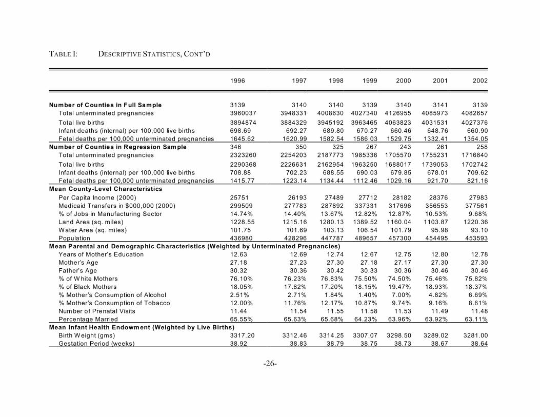
TABLE I: DESCRIPTIVE STATISTICS, CONT’D

1996 1997 1998 1999 2000 2001 2002

Number of Counties in Full Sample 3139 3140 3140 3139 3140 3141 3139





Number of Counties in Regression Sam ple 346 350 325 267 243 261 258





Mean County-Level Characteristics

Per Capita Income (2000) 25751 26193 27489 27712 28182 28376 27983

Medicaid Transfers in $000,000 (2000) 299509 277783 287892 337331 317696 356553 377561

% of Jobs in Manufacturing Sector 14.74% 14.40% 13.67% 12.82% 12.87% 10.53% 9.68%

Land Area (sq. miles) 1228.55 1215.16 1280.13 1389.52 1160.04 1103.87 1220.36

W ater Area (sq. miles) 101.75 101.69 103.13 106.54 101.79 95.98 93.10

Population 436980 428296 447787 489657 457300 454495 453593

Mean Parental and Demographic Characteristics (Weighted by Unterminated Pregnancies)

Years of Mother’s Education 12.63 12.69 12.74 12.67 12.75 12.80 12.78

Mother’s Age 27.18 27.23 27.30 27.18 27.17 27.30 27.30

Father’s Age 30.32 30.36 30.42 30.33 30.36 30.46 30.46

% of W hite Mothers 76.10% 76.23% 76.83% 75.50% 74.50% 75.46% 75.82%

% of Black Mothers 18.05% 17.82% 17.20% 18.15% 19.47% 18.93% 18.37%

% Mother’s Consumption of Alcohol 2.51% 2.71% 1.84% 1.40% 7.00% 4.82% 6.69%

% Mother’s Consumption of Tobacco 12.00% 11.76% 12.17% 10.87% 9.74% 9.16% 8.61%

Num ber of Prenatal Visits 11.44 11.54 11.55 11.58 11.53 11.49 11.48

Percentage Married 65.55% 65.63% 65.68% 64.23% 63.96% 63.92% 63.11%

Mean Infant Health Endowment (Weighted by Live Births)

Birth W eight (gms) 3317.20 3312.46 3314.25 3307.07 3298.50 3289.02 3281.00


-27-

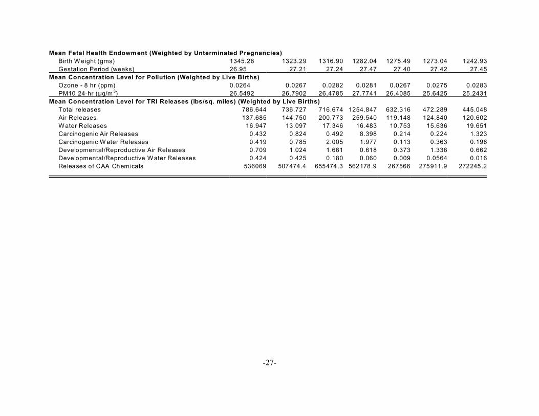
Mean Fetal Health Endowment (Weighted by Unterminated Pregnancies)

Birth W eight (gms) 1345.28 1323.29 1316.90 1282.04 1275.49 1273.04 1242.93


Mean Concentration Level for Pollution (Weighted by Live Births)

Ozone - 8 hr (ppm) 0.0264 0.0267 0.0282 0.0281 0.0267 0.0275 0.0283

PM10 24-hr (:g/m 3) 26.5492 26.7902 26.4785 27.7741 26.4085 25.6425 25.2431

Mean Concentration Level for TRI Releases (lbs/sq. miles) (Weighted by Live Births)

Total releases 786.644 736.727 716.674 1254.847 632.316 472.289 445.048

Air Releases 137.685 144.750 200.773 259.540 119.148 124.840 120.602

W ater Releases 16.947 13.097 17.346 16.483 10.753 15.636 19.651

Carcinogenic Air Releases 0.432 0.824 0.492 8.398 0.214 0.224 1.323

Carcinogenic W ater Releases 0.419 0.785 2.005 1.977 0.113 0.363 0.196

Developmental/Reproductive Air Releases 0.709 1.024 1.661 0.618 0.373 1.336 0.662

Developmental/Reproductive W ater Releases 0.424 0.425 0.180 0.060 0.009 0.0564 0.016

Releases of CAA Chem icals 536069 507474.4 655474.3 562178.9 267566 275911.9 272245.2

-28-

TABLE 2. CORRELATIONS OF TOXIC RELEASE CONCENTRATIONS WITH PARENT DEMOGRAPHICS AND COUNTY-LEVEL CONTROLS

Correlation of County and Aggregated Parental Factors with TRI concentrations net of Clean Air Act chemicals (lbs/sq. mile)

Mean PM10

(:g/m 3)

Mean ozone

(ppm)

Mother’s

Education

Mother’s Age Father’s Age Mother’s Race:

W hite

Air Releases 0.35% -9.82% 4.48% 5.38% 6.21% -4.61%

W ater Releases -1.48% -8.71% 2.58% 6.31% 6.69% -1.23%

Land Releases 0.07% -3.60% 0.51% -1.88% -1.96% -4.64%

Total Releases 0.07% -5.29% 1.30% -0.65% -0.58% -5.13%

Carcinogenic Air Releases 1.76% -3.06% 0.05% 2.02% 1.78% -9.01%

Carcinogenic Water Releases 0.37% -6.35% 1.62% 4.82% 4.88% -1.53%

Developmental/Reproductive Air Releases 0.35% -3.65% 1.19% -0.07% 1.88% -0.02%

Developmental/Reproductive W ater Releases -2.12% -4.47% 1.6% 3.13% 3.52% 1.22%

Releases of Clean Air Chemical 0.83% -10.28% -6.65% -0.34% 1.70% -8.21%

Mother’s

Race: Black

%Alcohol % Tobacco Prenatal Visits Married Per Capita

Income

Medicaid

Air Releases 3.62% -1.85% -0.52% -3.52% -2.17% 6.23% 3.05%

W ater Releases -0.40% -1.61% 0.98% -4.48% 1.00% 3.90% 0.30%

Land Releases 4.66% -1.25% -0.51% -4.13% -2.33% -0.26% 1.94%

Total Releases 4.93% -1.53% -0.53% -4.61% -2.50% 0.91% 2.32%

Carcinogenic Air Releases 5.25% -1.40% -1.74% -1.57% -4.64% 4.19% 0.72%

Carcinogenic Water Releases -0.47% -0.37% 0.05% -3.50% 1.47% 3.95% -0.96%

Developmental/Reproductive Air Releases 0.70% 0.13% 2.03% -0.33% -1.72% 0.74% 0.21%

Developmental/Reproductive W ater Releases -1.09% -0.41% 0.94% -3.59% -0.01% 1.05% -0.58%

Releases of Clean Air Chemical 8.31% -1.38% -3.84% -13.79% -14.71% -4.02% 18.51%

-29-

TABLE 3. WITHIN AND BETWEEN - COUNTY VARIATION FOR SELECT VARIABLES

Variable Mean

(Unweighted)

Standard Deviations

Overall Between W ithin

Total Births in County 7222.05 13584.87 11639.98 1336.74

Total Unterm inated Pregnancies in County 7311.89 13703.38 11768.90 1349.41

Infant deaths per 100,000 live births:

internal causes

748.62 306.63 233.69 227.18

Infant deaths per 100,000 live births:

external causes

33.89 61.39 65.16 52.77

Fetal Death per 100,000 unterminated

pregnancies

1248.19 1900.99 1854.18 507.56

County-Level Characteristics 26357.70 6114.64 6016.72 1789.94

Per Income Capital (2000 dollars) 290179.80 608665.10 560172.10 162925.50

Medicaid Transfer (2000 dollars) 14.19% 7.23% 7.84% 2.34%

% Employed in Manufacturing Industry 1767.33 16789.26 16752.40 6462.17

Parental and Demographic

Characteristics 19.63 145.12 127.69 100.95

% of W hite Mothers 2341.64 18330.51 18711.69 6727.84

% of Black Mothers 202.22 1447.13 1566.93 753.20

% of Mothers consuming Alcohol 1.14 13.42 11.12 10.32

% of Mothers consuming Tobacco 234.85 1543.28 1615.42 855.86

% Married 774.95 15239.38 14496.67 7090.34

Concentration Level for TRI Emission

(lbs/sq. mile) 0.56 15.62 16.15 8.64

Air Releases 190.65 650.98 578.31 393.04

W ater Releases 18.89 136.48 111.70 95.62

Total Releases 777.45 5402.16 5843.63 2441.41

Carcinogenic Air Releases 0.90 13.55 5.55 12.31

Carcinogenic Water Releases 1.03 11.81 8.66 9.30

Developmental/Reproductive Air Releases 1.40 26.48 12.61 22.34

Developmental/Reproductive W ater

Releases 0.58 16.12 16.15 8.90

Releases of Clean Air Chemical 1598.99 17142.10 16543.41 6639.82

-30-

TABLE 4. ESTIMATED EFFECTS OF AGGREGATE TRI CONCENTRATIONS ON MORTALITY

RATES

Variable ) Internal Infant Deaths ) Fetal Deaths (> 20 Weeks)

) TRI Concentrations (lbs/sq.mile) 0.00796* 0.00146

(0.00409) (0.00494)

) Mean PM10 (:g/m 3) -1.21146 -1.45204*

(0.94310) (0.80748)

) Mean Ozone (ppm) 752.32926 -523.20385

(1,326.81966) (1,306.33806)

) Maternal Tobacco Use -45.76362 70.19407**

(35.81560) (29.82474)

) Maternal Alcohol Use -28.17296 81.99949*

(46.92025) (42.66148)

) Per Capita Income Y Y

) Medicaid Y Y

) Other Parent Demographics Y Y

Year Indicators Y Y

State -Year Indicators Y Y

Observations 3895 3895

R-squared 0.21 0.19

Robust standard errors in parentheses

* significant at 10%; ** significant at 5%; *** significant at 1%

Note: Internal mortality rates are per 100,000 births and fetal mortality rates are per 100,000 pregnancies. Internal infant

mortality regressions are weighted by total number of births in each county and year. Fetal mortality regression is

weighted by total number of pregnancies in each county and year.

-31-

TABLE 5. ESTIMATED EFFECTS OF TRI CONCENTRATIONS BY MEDIA ON MORTALITY

RATES


) TRI Air (lbs/sq. mile) 0.02312** 0.01121

(0.01003) (0.01227)

) TRI W ater (lbs/sq. mile) -0.00866 -0.03404

(0.04952) (0.04620)

) TRI Land (lbs/sq. mile) 0.00484 0.00016

(0.00486) (0.00608)

) Mean PM10 (:g/m 3) -1.21164 -1.46100*

(0.94443) (0.80721)

) Mean Ozone (ppm) 733.22040 -527.70335

(1,325.91786) (1,305.25042)


(35.69114) (30.05122)


(46.99218) (42.68681)


) Medicaid Y Y


Year Indicators Y Y



R-squared 0.21 0.19



Note: Internal mortality rates are per 100,000 b irths and fetal mortality rates are per 100 ,000 pregnancies. Internal infant



-32-

TABLE 6. ESTIMATED EFFECTS OF TRI CONCENTRATIONS BY MEDIA AND TYPE ON MORTALITY

RATES


) TRI Developmental/Reproductive

Toxins: Air (lbs/sq. mile)

-0.06861 -0.22194**

(0.10630) (0.09268)

) TRI Carcinogens: Air (lbs/sq. mile) 0.33127** 0.01375

(0.15189) (0.26905)

) TRI Other: Air (lbs/sq. mile) 0.00319 0.00159

(0.00978) (0.01171)

) TRI Developmental/Reproductive

Toxins: W ater (lbs/sq. mile)

-0.65850** -0.55733

(0.26058) (0.35560)

) TRI Carcinogens: Water (lbs/sq. mile) 0.23693 0.05050

(0.25344) (0.36044)

) TRI Other: W ater (lbs/sq. mile) 0.02063 -0.00421

(0.03269) (0.07323)

) TRI Developmental/Reproductive:

Land (lbs/sq. mile)

0.10165 -0.39360

(0.21038) (0.28557)

) TRI Carcinogens: Land (lbs/sq. mile) 0.00780 0.00579

(0.00961) (0.01183)

) TRI Other: Land (lbs/sq. mile) 0.00522 0.00004

(0.00504) (0.00601)

) Mean PM10 (:g/m 3) -1.18709 -1.45647*

(0.94594) (0.80470)

) Mean Ozone (ppm) 543.62941 -314.08287

(1,357.83770) (1,305.96114)


(35.78864) (30.31320)


(47.24545) (42.69350)


) Medicaid Y Y


Year Indicators Y Y



R-squared 0.21 0.19



Note: Internal mortality rates are per 100,000 births and fetal mortality rates are per 100,000 pregnancies. Internal infant



-33-

TABLE 7. ESTIMATED ELASTICITIES AND LIVES SAVED OR LOST: AVERAGE ANNUAL COUNTY-LEVEL VALUES

Variable Mean

(lbs/sq. mile)

Mean Change

in

Concentration

Estimated

$Standard

Error

Aggregate:

Point Estimate of

Lives Lost (Saved)

Aggregate:

Low Estimate of

Lives Lost (Saved)

Aggregate:

High Estimate of

Lives Lost (Saved)

Total 673.2810 -1.20% 0.0080 0.0040 -25237 -49969 -505

Air 169.4333 -4.86% 0.0230 0.0100 -73776 -136645 -10906

W ater 17.2978 -4.57% -0.0090 0.0500 2769 -27374 32910

Carcinogenic Air 1.1702 0.84% 0.3310 0.1500 1264 831 6500

Developmental or

Reproductive W ater

0.2060 -6.94% -0.6590 0.2600 3666 -1732 5340

Mean Internal Deaths (per 100,000 live births) 775.6

Total Births (000,000) 27.8

Total Pregnancies (000,000) 28.1

-34-

FIGURE 1. AVERAGE ANNUAL COUNTY-LEVEL INTERNAL INFANT DEATH RATE PER 100,000LIVE BIRTHS BY TRI QUARTILE

-35-

FIGURE 2. AVERAGE ANNUAL COUNTY-LEVEL FETAL DEATH RATE PER 100,000 LIVE BIRTHS

BY TRI QUARTILE (> 20 WEEKS GESTATION)

-36-

FIGURE 3. AGGREGATE TRI RELEASES BY MEDIA

-37-

FIGURE 4. AGGREGATE TRI AIR RELEASES BY TYPE

-38-

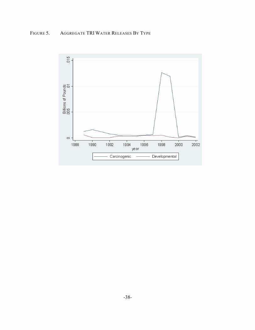
FIGURE 5. AGGREGATE TRI WATER RELEASES BY TYPE

-39-

FIGURE 6. AVERAGE ANNUAL COUNTY-LEVEL TRI CONCENTRATION BY MEDIA

-40-

FIGURE 7. AVERAGE ANNUAL COUNTY-LEVEL TRI AIR CONCENTRATION BY TYPE

-41-

FIGURE 8. AVERAGE ANNUAL COUNTY-LEVEL TRI WATER CONCENTRATION BY TYPE

Documents

PRELIMINARY: Please do not cite or quote without permission · And, within air pollution, releases of carcinogens a re particu larly problema tic for infant health outcomes. We do