Prediction of Second Virial Coefficients from Intrinsic Viscosities

CHONG MENG KOK* and ALFRED RUDIN, Guelph- Waterloo Centre for Graduate Work i n Chemistry, Department of Chemistry, University of

Waterloo, Waterloo, Ontario, Canada N2L 3G1

Synopsis

One of the most readily available characteristics of a polymer sample is its intrinsic viscosity in a particular solvent. This datum can often be estimated reasonably from a single relative viscosity measurement. A number of theories permit the calculation of the second virial coefficient of a polymer/solvent mixture given the intrinsic viscosity and polymer molecular weight. The intrinsic viscoSity of the polymer under theta conditions is also needed, but this can be estimated, if necessary, from the molecular weight. This article compares the efficiencies of various alternative models for the prediction of second virial coefficients of a series of polymers and solvents. The most effective technique for this purpose first calculates the concentration-dependent equivalent hydrodynamic volume of a solvated polymer coil. This value is used with a primitive statistical mechanical theory for virial coefficients of hard-sphere suspensions to calculate the osmotic pressure or turbidity of the polymer solution. These simulated experimental values are fitted with a least-squares line as in the real experiment, and the second virial coefficient is derived from the slope. The computations are relatively simple; the average deviation between observed and predicted virial coefficients was less than 16% for a variety of polymer types, molecular weights, and solvents.

INTRODUCTION

A polymer solution theory can be assessed by its ability to predict experimental results. A group of theories has evolved from consideration of the excluded volume effect. These are now often referred to as the two-parameter theory.' Two-parameter theories relate dilute polymer solution properties to two basic parameters, i.e., the mean-square end-to-end distance ( r ) o of a chain in the theta state and the excluded volume parameter z .

The Yamakawa theory2 is an example of a two-parameter theory. Recently, Mahabadi and Rudin3 have shown that this model can be used to explain the change in elution volumes with concentrations of polymer solutions in gel per- meation chromatography (GPC). In our experience, the Yamakawa theory appears to give the best agreement with experimental results when compared to the other two-parameter theories.

In a different approach, Rudin3v4 has proposed a model to account for the concentration dependence of equivalent hydrodynamic volumes of polymer solutions. Although it is simple in derivation, this theory has been shown to be capable of accounting for a modest variety of polymer solution properties. It has given correct estimations of radii of gyration in solution: corrected for concentration effects in GPC,3,4 explained peak shifts in GPC of polymer mix- t u r e ~ , ~ and predicted osmotic pressures of polymer solutions.6

The second virial coefficient is a very important characteristic of polymer

* On leave from Universiti Sains, Penang, Malaysia.

Journal of Applied Polymer Science, Vol. 26,3583-3597 (1981) 0 1981 John Wiley & Sons, Inc. CCC 0021-8995/81/113583-15$01.50

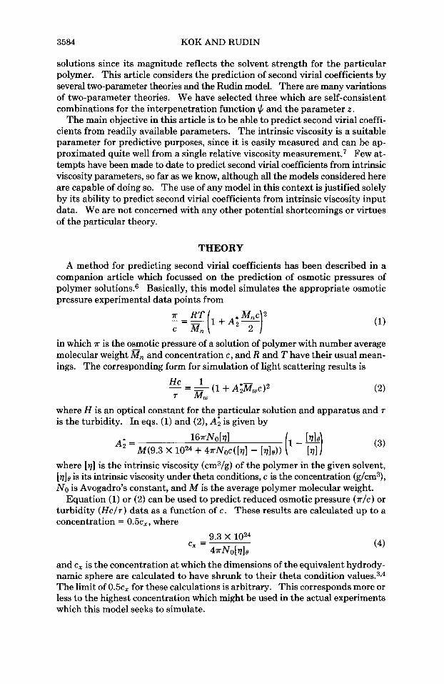
3584 KOK AND RUDIN

solutions since its magnitude reflects the solvent strength for the particular polymer. This article considers the prediction of second virial coefficients by several two-parameter theories and the Rudin model. There are many variations of two-parameter theories. We have selected three which are self-consistent combinations for the interpenetration function Ic/ and the parameter z .

The main objective in this article is to be able to predict second virial coeffi- cients from readily available parameters. The intrinsic viscosity is a suitable parameter for predictive purposes, since it is easily measured and can be ap- proximated quite well from a single relative viscosity mea~urernent.~ Few at- tempts have been made to date to predict second virial coefficients from intrinsic viscosity parameters, so far as we know, although all the models considered here are capable of doing so. The use of any model in this context is justified solely by its ability to predict second virial coefficients from intrinsic viscosity input data. We are not concerned with any other potential shortcomings or virtues of the particular theory.

THEORY

A method for predicting second virial coefficients has been described in a companion article which focussed on the prediction of osmotic pressures of polymer solutions.6 Basically, this model simulates the appropriate osmotic pressure experimental data points from

T RT

in which 7r is the osmotic pressure of a solution of polymer with number average molecular weight an and concentration c, and R and T have their usual mean- ings. The corresponding form for simulation of light scattering results is

- (1+A;Mwc)2 7- XIw

where H is an optical constant for the particular solution and apparatus and r is the turbidity. In eqs. (1) and (2), AH is given by

where [q] is the intrinsic viscosity (cm3/g) of the polymer in the given solvent, [&I is its intrinsic viscosity under theta conditions, c is the concentration (g/cm3), No is Avogadro’s constant, and M is the average polymer molecular weight.

Equation (1) or (2) can be used to predict reduced osmotic pressure (a/c) or turbidity (Hc/r) data as a function of c. These results are calculated up to a concentration = 0 . 5 ~ ~ ~ where

9.3 x 1024 47rN0 hl c, = (4)

and c, is the concentration at which the dimensions of the equivalent hydrody- namic sphere are calculated to have shrunk to their theta condition value^.^.^ The limit of 0 . 5 ~ ~ for these calculations is arbitrary. This corresponds more or less to the highest concentration which might be used in the actual experiments which this model seeks to simulate.

SECOND VIRIAL COEFFICIENTS 3585

The ostensible virial coefficients A ; in eqs. (1) and (2) are concentration de- pendent because they are related to the radius of the equivalent hydrodynamic sphere which decreases in size with increasing concentration in the concentration region 0 I c 5 c,. To obtain a concentration-independent second virial coef- ficient, Az, from this model, one plots ( a / ~ ) l / ~ [eq. (l)] or ( H c / T ) ~ / ~ [eq. (2)] against c for 0 I c I 0 . 5 ~ ~ and fits a least-squares line to the results to derive A2 from the slope.

This theory differs from the others considered here in that it involves a direct simulation of raw experimental data points which are then handled exactly as in the real experiment to predict the second virial coefficient of the particular polymer solution.6 It will be referred to below as the KR model.

In the two-parameter theory, the second virial coefficient can be written as'

in which

1c/ = ZhO(2) (6)

2 = z / a : (7)

a: = (S2) / (S2)0 (8)

and

In the above expressions, (S2) is the mean square radius of gyration and (S2)o is the value of ( S2) under theta conditions.

Various forms of the interpenetration function $ have been developed. An appropriate expression for z must be selected for each function of 1c/ such that their derivations are based on the same footing in terms of intramolecular and intermolecular theories of interaction. Three such combinations suggested by Yamakawal are used in the present study. These are:

Flory-Krigbaum-Orofino theory8 of 1c/ (FKO): Combination 1:

(9) In (1 + 2.302) ' = 2.30

Flory theory of a,: a," - a: = 2.602 (10)

Combination 2: Modified Flory-Krigbaum-Orofino theoryl0 of 1c/ (MFKO):

(11) In (1 + 5.732)

lc/ = 5.73 Modified Flory theoryll of as:

- = 1.2762 (12)

Combination 3: Kurata-Yamakawa theory12 of 1c/ (KY):

= 0.547[1 - (1 + 3.9032)-0.4683] (13) Yamakawa-Tanaka theory13 of a,:

3586 KOK AND RUDIN

a: = 0.541 + 0.459(1 + 6 . 0 4 ~ ) O . ~ ~ (14)

In order to use these theories for the estimation of A2 from intrinsic viscosity data, it is necessary to make use of equations which do not involve the various radii of gyration. The following relationships of Flory and Foxl4J5 are useful for this purpose:

and

The proportionality constant @O is considered below. It appears in all the two-parameter theories and is included in the KR model as ell.^^^ Elimination of ( S2) 3/2 in eq. (5) leads to

To estimate a value for A2, \t must be caculated according to one of the above theories. Taking combination 3 as an example, one first obtains a, from eq. (16). Substitution of this value of as into eq. (14) gives z , and Z is then obtained from eq. (7). This is then used in eq. (13) to estimate \t, and the latter value is finally put into eq. (17) to calculate Az.

Various theoretical values of are available. However, a common value which is often obtained is 2.5 X loz3 (with [q] and ( S ) in cgs units).15

It is not our intention here to discuss the validity of the various theories of polymer solution behavior. We are solely concerned with the efficiency of these models in the prediction of second virial coefficients using intrinsic viscosities as the input parameters. So far as we know, this application of these particular theories has not been considered explicitly before.

RESULTS

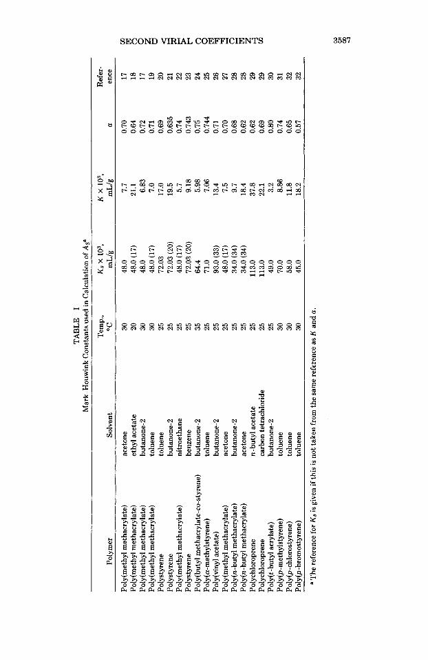
The theories mentioned above were used to predict second virial coefficients for about 140 polymer samples for which apparently reliable A2 values were lo- cated in the literature. In most cases, the samples selected were fractions with fairly sharp molecular weight distributions. The intrinsic viscosities were cal- culated from the appropriate Mark-Houwink relations:

[q] = KMt (18)

The Mark-Houwink constants used are listed in Table I. It is not possible to present Az values calculated from all three two-parameter

theories because of space limitations. Results from the Kurata-Yamakawa (KY) theory have been selected for illustrative purposes, while an overall comparison with the other two models is given below.

Predicted and experimental A2 values obtained from the KY theory and the

TA

BL

E

I M

ark-

Hou

win

k C

onst

ants

use

d in

Cal

cula

tion

of A

ze

Tem

p.,

K~ x

103

, K

x 10

3,

Ref

er-

Poly

mer

So

lven

t "C

m

L/g

m

L/g

a

ence

Poly

(met

hy1 m

etha

cryl

ate)

Po

ly(m

ethy

1 met

hacr

ylat

e)

Poly

(met

hy1 m

etha

cryl

ate)

Po

ly(m

ethy

1 met

hacr

ylat

e)

Poly

styr

ene

Poly

styr

ene

Poly

(met

hy1 m

etha

cryl

ate)

Po

lyst

yren

e Po

ly(b

uty1

met

hacr

ylat

e-co

-sty

rene

) Po

ly (a

-met

hyls

tyre

ne)

Poly

(vin

y1 ac

etat

e)

Poly

(met

hy1 m

etha

cryl

ate)

Po

ly(n

-but

yl m

etha

cryl

ate)

Po

ly(n

-but

yl m

etha

cryl

ate)

Po

lych

loro

pren

e Po

lych

loro

pren

e Po

ly(t

-but

yl a

cryl

ate)

Po

ly(p

-met

hyls

tyre

ne)

Poly

(pch

1oro

styr

ene)

Po

ly@

-bro

mos

tyre

ne)

acet

one

ethy

l ace

tate

bu

tano

ne-2

to

luen

e to

luen

e bu

tano

ne-2

ni

troe

than

e be

nzen

e hu

tano

ne-2

to

luen

e bu

tano

ne-2

ac

eton

e bu

tano

ne-2

ac

eton

e n-

buty

l ace

tate

ca

rbon

tetr

achl

orid

e bu

tano

ne-2

to

luen

e to

luen

e

30

20

30

30

25

25

25

25

35

25

25

25

25

25

25

25

25

30

30

48.0

48

.0 (

17)

48.0

48

.0 (

17)

72.0

3 72

.03

(20)

48

.0 (1

7)

72.0

3 (2

0)

64.4

71

.0

93.0

(33

) 48

.0 (

17)

34.0

(34

) 34

.0 (

34)

113.

0 11

3.0

49.0

70

.0

58.0

7.7

21.1

6.

83

7.0

17.0

19

.5

5.7

9.18

5.

98

7.06

13

.4

7.5

9.7

18.4

37

.8

22.1

3.

2 8.

86

11.8

0.70

0.

64

0.72

0.

71

0.69

0.

635

0.74

0.

743

0.75

' 0.

744

0.71

0.

70

0.68

0.

62

0.62

0.

69

0.80

0.

74

0.65

rn M

18

0

17

0

17

19

3 21

5

22

E 23

E

26

# E! t3

20

24

0

25

0

27

Fi 28

Q

28

29

29

30

31

32

tolu

ene

30

45.0

18

.2

0.57

32

a T

he re

fere

nce

for K

e is

giv

en if

thi

s is

not

take

n fr

om th

e sa

me

refe

renc

e as

K a

nd a

.

3588

I

KOK AND RUDIN

A I I I I

4.7 4.9 5.7 5.3 5.5 5.7 6.9

lop M

Fig. 1. Osmotic second virial coefficients for poly(methy1 methacrylate) in acetone: (0) experi- mentall'; (0) K R (A) KY. The line joins experimental points.

KR model are presented in Figures 1-18. Most of the experimental values are obtained from light scattering measurements. In general, the KFi model provides a somewhat better prediction than the KY theory, which estimates virial coef- ficients which are too small in most cases. This is especially apparent for lower-molecular-weight samples in Figures 2,3,6,8-13,16, and 17. In Figure 4, however, which deals with very high-molecular-weight polymers, the KY theory

log M

Fig. 2. Light scattering second virial coefficients for poly(methy1 methacrylate) in butanone-2.22 Symbols same as in Fig. 1.

Y 0 4

t 0 x (u

U I

Fig. 3. Light scattering second virial coefficients for poly(methy1 methacrylate) in nitroethane.22 Symbols same as in Fig. 1.

SECOND VIRIAL COEFFICIENTS 3589

predictions are almost exact. Some of the predicted A2 values from the KR theory are higher than experimental figures, as in Figures 14,15, and 18.

4 r

* *

2 4 6 8 I0 12 14 - 0

M w x tV6 Fig. 4. Light scattering second virial coefficients for high-molecular-weight polystyrenes in ben-

~ e n e . ~ ~ Symbols same as in Fig. 1.

'cm 5 1 4 N

5.2 5.3 5.4 5.5 5.6 5.7 5.8 tog M

Fig. 5. Light scattering second virial coefficients of poly(buty1 methacrylate-co-styrene) in bu- tan0ne-2.~~ Symbols same as in Fig. 1.

l o g M

Fig. 6. Second virial coefficients from equilibrium sedimentation measurementP for polystyrenes in benzene. The predicted values are for light scattering. Symbols same as in Fig. 1.

3590 KOK AND RUDIN

41-

(v I

b

X

b

I -

~

5.3 5.5 5.7 5 9 6.1 6.3 6.5 6.1 69

t o g M

Fig. 7. Light scattering second virial coefficients for high-molecular-weight poly(cu-methylstyrenes) in toluene.37 Symbols same as in Fig. 1.

A further comparison of the two theories is provided by the osmotic pressure data of Vink40 for a variety of polymers in various solvents. These are generally high-concentration experimental points. The KR theory produces a noticeably better fit to the experimental A2 values than the KY model, as shown in Table 11.

A comparison of the predictions of the four methods is given in Figures 19-22 which show plots of predicted versus experimental A2 values for all the systems examined. One can judge the merit of each prediction by noting the scatter about the line drawn through the origin with a slope of unity. The two-parameter theories appear to give poor predictions for experimental values of A2 greater than 3 X cm3.mol/g2. Generally speaking, this means that the two-pa- rameter theories give good predictions only if the molecular weight is greater than 106.

A quantitative comparison of the above theories can be obtained by calculating the average percentage error over the 140 experimental data examined. Data in which the Mark-Houwink constants are not applicable because the polymer has too low a molecular weight are not taken into consideration. An apparent aberrant data point at log M = 5.7 in Figure 5 is also not used. The average percentage error for each theory is calculated according to

n

I 2 *;

A

I I I I I I I J 4.5 4.1 4.9 5.1 5.3 5.5 5.1 5.9

log M Fig. 8. Light scattering second virial coefficients for lower-molecular-weight samples of poly(cu-

methylstyrene) in tol~ene.3~ (The experimental A2 for molecular weight 39,300 has not been used because the original authors reported that its [v] was abnormal.) Symbols same as in Fig. 1.

SECOND VIRIAL COEFFICIENTS

I

3591

. I I I I I I I

4.-

“ t i , I I I I , a 5.9 6.0 6.1 6.2 6.3 6.4 6.5 6.6

log M

Fig. 9. Light scattering second virial coefficients for poly(viny1 acetate) in butanone-2?6 Symbols same as in Fig. 1.

N I experimental - predicted 1 c experimental (20) N

where A’ is the number (= 140) of experimental data. (Note that only the ab- solute deviations between predicted and experimental A2 values are taken into account).

1 average percentage error =

2 ;; 4.9 5.1 5.3 5.5 5.7 5.9 6.1 6.3

Oog M

Fig. 10. Light scattering second virial coefficients for poly(methy1 methacrylate) in acetone.27 Symbols same as in Fig. 1.

r

3592

2

KOK AND RUDIN

4-

0

3- 0

-A b-\ A 0

A A I -

I I I I I I 1

1 I I I I I I I 1 1 8.0 5.1 5.2 5.3 5.4 5.5 5.6 5.7 5.8

top M Fig. 12. Light scattering second virial coefficients for poly(n-butyl methacrylate) in butanone-2.%

Symbols same as in Fig. 1.

The percent errors obtained for the KR, KY, FKO, and the MFKO theories are 15.6, 25.8, 32.9, and 22.3, respectively.

DISCUSSION The above results show that the KR model gives generally good predictions

of second virial coefficients for a variety of solvents and polymers with different molecular weights. This is convenient, since the estimation of virial coefficients involves simple mathematics in this case.

I I I 1 I I I I 5.0 5.1 5.2 5.3 5.4 5.5 5.6 5.7 5.8

fog M Fig. 13. Light scattering second virial coefficients for poly(n-butyl methacrylate) in acetone.28

Symbols same as in Fig.

N 'm

2 n E 0 * P X N

U

1.

Fig. 14. Light scattering second virial coefficients for polychloroprene in n-butyl acetate.39 Symbols same as in Fig. I.

SECOND VIRIAL COEFFICIENTS 3593

1 I I I I I I I ( 5.1 5.3 5.5 5.7 5.9 6.1 63 6.5

log M

Fig. 15. Light scattering second virial coefficients for polychloroprene in carbon tetrachl~ride.~~ Symbols same as in Fig. 1.

The comparisons in this article are based on the use of intrinsic viscosities as input parameters. We are not concerned with the validity of eqs. (15) and (161, in general. However, since the two-parameter theories rely on these relation-

I t I I I I I I I I

4.8 4.9 5.0 5.1 5.2 5.3 5.4 5.5

log M Fig. 16. Light scattering second virial coefficients for poly(t -butyl acrylate) in b~tanone-2 .~~

Symbols same as in Fig. 1.

01

- 3 A

E 0 2

n

52 5.4 5.6 5.8 6.0 6.2 6.4 Log M

Fig. 17. Light scattering second virial coefficients .for poly(p-methyl styrene) in toluene.31 Symbols same as in Fig. 1.

3594 KOK AND RUDIN

N

0 a . 9 . . x r 0 I I t 1 I I 5.3 5.5 5.7 5.9 6.7 6.3 6.5 6.7

log M

Fig. 18. Light scattering second virial coefficients for poly(p-chlorostyrene) in toluene (upper line) and poly(p-bromostyrene) in toluene (lower line).32 Symbols same as in Fig. 1.

ships, one should examine the possible improvements in prediction of experi- mental results when the parameters in these equations are adjusted judiciously. Equation (15) can be changed by using a lower value of the Flory universal con- stant @o, as this will increase the value of A2 estimated by the two-parameter models. An alternative value for this constant is %O = 2.1 X (in cgs units), which is an experimental value often quoted for polydisperse polymers.33 Also, the equality in eq. (16) can be replaced by4I

(21) & 3 = 2 4 3 7J a s .

We have made these substitutions into the calculations, and the average percent errors are shown in Table 111. Under the last conditions shown the predictions of the KY theory are improved substantially, while those of the other two-parameter models are not altered for the better. The original Rudin model4 used @o = 2.1 X 1021 (actually, the Flory constant labelled 4’ was set a t 63/2%0). Substitution of @O = 2.5 X 1021 into the formulas for hydrodynamic volume and cx produces A2 estimates with an average error of 16.8% for this model.

K r i g b a ~ m ~ ~ suggested the following empirical relation between A2 and in- trinsic viscosities:

TABLE I1 Second Virial Coefficient from Vink’s Data40

Molecular A2 X lo4 cm3.mol/g2 (osmotic) Polymer/Solvent weight Experimental KR Theory KY Theory

PMMA/toluene 89,800 2.65 2.58 1.51 PMMA/acetone 95,600 2.42 2.45 1.39 PMMA/ethyl acetate 103,900 2.82 4.02 2.58 PMMAbutanone-2 100,800 3.24 3.01 1.78 PS/toluene 119,300 5.59 5.65 3.50 PSbutanone-2 550,000 1.41 1.60 0.90

SECOND VIRIAL COEFFICIENTS 3595

N

* 0 4 -

0

0

o o o o o 0

I 2 3 4 5 6 0 7

EXPERIMENTAL A2 x 104cm3 rnd g-2

Fig. 19. Comparison of predicted and experimental A2 values for all the systems studied. The predicted values are from the FKO theory.

TABLE I11 Average Percent Errors of Various Theories

a. x 10-23, Relation between Average % error ces units a. and a, KR KY FKO M F K ~

2.5 a, = a? 16.8 25.8 32.9 22.3 2.1 ff, = ff? 15.6 18.6 30.4 21.6 2.5 = ffy 16.8 21.5 31.5 21.5 2.1 = &43 15.6 17.6 35.3 27.0

With the data uszd in this study eq. (22) gives an average percent error of 24.9% with 90 = 2.1 X 1021 and an error of 19.2% with 9 0 = 2.5 X lo2' (in cgs units). This relation involves less computation than any of those considered here and produces estimates in reasonable accord with experimental values.

The model described in this and the preceding article on this topic6 appears

Fig. 20. Comparison of predicted and experimental A2 values for all the systems reported above. The predicted values are from the MFKO theory.

3596 KOK AND RUDIN

Fig. 21. Comparison of predicted and experimental A2 values for all the systems reported above. The predicted values are from the KY theory.

to provide the best overall estimates of second virial coefficients for a variety of polymer-solvent combinations (cf. Table I1 and Fig. 22). It consists essentially of a calculation of a concentration-dependent equivalent hydrodynamic volume for a solvated polymer coil and use of this volume in a primitive statistical me- chanical theory for virial coefficients of hard sphere suspensions. It cannot possibly accord with all the characteristics of real polymer solutions, but it can nevertheless serve as a very useful predictive tool despite this limitation.

We have used a model proposed by one of us4 to estimate the equivalent di- mensions of polymers in solution. Any other theory which predicts these di- mensions correctly could be employed equally as well to provide input data for the statistical mechanical dilute suspension model.16 Thus, it is expected3 that replacement of Rudin’s model with Yamakawa’s expressions for the concen- tration dependence of the sizes of equivalent hydrodynamic spheres2 would produce equivalent A2 values with eqs. (1) or (2) and eq. (3).

0 O / ? 6 - 0 - e 5 -

3

2 3 -

* 4 - Q x

0

E 2 -

I I I I I I t I 2 3 4 5 6 r

EXPERIMENTAL A2 x lo4 cm3 mot g-2

r

? 6 0 - e 5

3

2 3

* 4 Q x

0

E 2

0 I 2 3 4 5 6 r EXPERIMENTAL A2 x lo4 cm3 mot g-2

Fig. 22. Comparison of predicted and experimental A2 values for all the systems reported above. The predicted values are from the KR theory given in this article.

SECOND VIRIAL COEFFICIENTS 3597

Since the present method simulates the results of the actual experiment from which A2 is derived, it can also be used to predict colligative properties or tur- bidity of polymer solutions, as outlined earlier6 for osmotic pressure values in particular.

This work was supported by the Natural Sciences and Engineering Research Council of Canada.

References

1. H. Yamakawa, Modern Theory of Polymer Solutions, Harper and Row, New York, 1971. 2. H. Yamakawa, J. Chem. Phys., 43,1334 (1965). 3. H. K. Mahabadi and A. Rudin, Polym. J. (Japan), 11,123 (1979). 4. A. Rudin and R. A. Wagner, J. Appl. Polym. Sci., 20,1483 (1976). 5. C. M. Kok and A. Rudin, Makromol. Chem., to appear. 6. C. M. Kok and A. Rudin, J. Appl. Polym. Sci., 26,3575 (1981). 7. A. Rudin and R. A. Wagner, J. Appl. Polym. Sci., 19,3361 (1975). 8. P. J. Flory and W. R. Krigbaum, J. Chem. Phys., 18.1086 (1950); T. A. Orofino and P. J. Flory,

9. P. J. Flory, J. Chem Phys., 17,303 (1949). ibid., 26,1067 (1957).

10. W. H. Stockmayer, Makromol. Chem., 35,54 (1960). 11. W. H. Stockmayer, J. Polym. Sci., 15,595 (1955). 12. H. Yamakawa, J. Chem. Phys., 48,2103 (1968). 13. H. Yamakawa and G. Tanaka, J. Chem. Phys., 47,3991 (1967). 14. P. J. Flory, J. Chem. Phys., 17,303 (1949). 15. P. J. Flory and T. G. Fox, J. Am. Chem. SOC., 73,1904 (1951). 16. B. H. Zimm, J. Chem. Phys., 14,164 (1946). 17. T. G. Fox, J. B. Kinsinger, H. F. Mason, and E. M. Schuele, Polymer (London), 10, 71

18. A. F. V. Eriksson, Acta Chem. Scand., 10,378 (1956). 19. E. Cohn-Ginsberg, T. G. Fox, and H. F. Mason, Polymer (London), 10,97 (1962). 20. P. Outer, C. I. Carr, and B. A. Zimm, J. Chem. Phys., 18,830 (1950). 21. J. 0 t h and Y. Desreux, Bull. SOC. Chim. Belg., 18,830 (1954). 22. E. F. Casassa and W. H. Stockmayer, Polymer, 3,53 (1962). 23. T. A. Orofino and F. Wenger, J. Phys. Chem., 67,566 (1963). 24. K. S. V. Srinivasan and M. Santappa, J. Polym. Sci. Polym. Phys. 11,331 (1973). 25. I. Noda, K. Mizutai, T. Kato, T. Fujimoto, and M. Nagasawa, Macromolecules, 3, 787

26. A. R. Shultz, J. Am. Chem. SOC., 76,3423 (1954). 27. J. Bischoff and V. Desreux, Bull. SOC. Chim. Belges, 61,lO (1952). 28. R. Van Leempont and R. Stein, J. Polym. Sci., Al, 985 (1963). 29. K. Kawahara, T. Norisuye, and H. Fujita, J. Chem. Phys., 49,4339 (1968). 30. R. Jerome and V. Desreux, Eur. Polym. J., 6,411 (1970). 31. G. Tanaka, S. Imai, and H. Yamakawa, J. Chem. Phys., 52,2639 (1970). 32. Y. Noguchi, A. Aoki, G. Tanaka, and H. Yamakawa, J. Chem. Phys., 52,2651 (1970). 33. M. Kurata and W. H. Stockmayer, Fortschr. Hochpolym. Forsch., 3,196 (1963). 34. S. N. Chinai and R. A. Guzzi, J. Polym. Sci., 21,417 (1956). 35. M. Fukuda, M. Fukutoni, Y. Kato, and T. Hashimoto, J. Polym. Sci. Polym. Phys., 12,871

36. S. G. Chu and P. Munk, J. Polym. Sci. Polym. Phys., 15,1163 (1977). 37. T. Kato, M. Miyaso, I. Noda, T. Fujimoto, and M. Nagasawa, Macromolecules, 3, 777

38. G. V. Schulz and H. Bauman, Makromol. Chem., 114,122 (1968). 39. T. Norisuye, K. Kawahara, A. Teramoto, and H. Fujita, J. Chem. Phys., 49,4336 (1968). 40. H. Vink, Eur. Polym. J., 10,149 (1974). 41. M. Kurata and H. Yamakawa, J. Chem. Phys., 29,311 (1958). 42. W. R. Krigbaum, J. Polym. Sci., 18,315 (1955).

(1962).

(1970).

(1974).

(1970).

Received November 10,1980 Accepted December 18,1980