Embed Size (px)
Citation preview
Predicting the type of shopper (weekend or weekday) from
online grocery data.
Luc Majoor
ANR: 509836
Master Thesis
Thesis submitted in partial fulfilment of the requirements for the degree of Master of Science in
Communication and Information Sciences, Master Track Data Science: Business and Governance, at
the School of humanities of Tilburg University
Thesis committee:
Supervisor: Dr. F. Hermens
Second reader: Dr. M. Postma
Tilburg University
School of Humanities
Department of Communication and Information Sciences
October, 2018
2
Preface
The thesis “Predicting the type of shopper (weekend or weekday) from online grocery data” has been
written as partial fulfilment of the requirements for the Master Track Data Science: Business and
Governance at Tilburg University. I was engaged in researching and writing this thesis from January
2018 to October 2018. My research questions were formulated together with my supervisor at Tilburg
University, Dr. F. Hermens. I would like to thank Frouke for the excellent guidance and support
during this process. Finally, it must be said that the support of family and friends was enormous and
led to an even greater enthusiasm and thrive to complete this thesis.
Luc Majoor
Tilburg, October 2018
3
Predicting the type of shopper (weekend or weekday) from online grocery data.
Majoor, L.
Tilburg University
Abstract
Online grocery retailing, also known as e-grocery, is a type of business-to-consumer e-commerce that
has enjoyed great growth in the last decade and is expected to continue to grow in the years to come.
To avoid out-of-stock situations and food waste, it is therefore becoming increasingly important to
understand the purchasing patterns and predict demand. Studies of offline shopping patterns have
suggested that weekend and weekday shoppers differ in their purchasing patterns, but it is unclear
whether such patterns extend to online shopping, because of the relative ease of an online shop. By
analysing a large database of online grocery orders, it was found that online orders show a clear
difference between weekdays and weekends, providing a clear means to ensure sufficient stocks and
avoid waste.
Keywords: online grocery shopping, machine learning, retail, type of shopper, weekend, weekday
4
Contents
1 INTRODUCTION .............................................................................................................................................. 5
1.1 CONTEXT ................................................................................................................................................ 5
1.1.1 Online Grocery Shopping ...................................................................................................................... 5
1.1.2 Practical relevance ................................................................................................................................ 9
1.1.3 Scientific relevance .............................................................................................................................. 10
1.2 RESEARCH QUESTIONS ................................................................................................................................. 11
1.3 STRUCTURE ................................................................................................................................................. 12
2 RELATED WORK .......................................................................................................................................... 12
2.1 TYPOLOGY OF GROCERY SHOPPERS ............................................................................................................. 12
2.2 TIME OF PURCHASE ...................................................................................................................................... 14
2.3 DATA MINING TECHNIQUES .......................................................................................................................... 15
2.4 VARIABLE SELECTION .................................................................................................................................. 18
2.5 RESEARCH GAP ............................................................................................................................................ 19
3 METHOD ......................................................................................................................................................... 20
3.1 DATASET ..................................................................................................................................................... 20
3.1.1 Description .......................................................................................................................................... 20
3.1.2 Instacart .............................................................................................................................................. 21
3.1.3 Programming language ....................................................................................................................... 22
3.2 PRE-PROCESSING ......................................................................................................................................... 22
3.3 FEATURE ENGINEERING ............................................................................................................................... 23
3.3.1 Feature selection ................................................................................................................................. 23
3.3.2 Feature construction ........................................................................................................................... 23
3.4 EXPERIMENTAL PROCEDURE ........................................................................................................................ 25
3.5 EVALUATION CRITERIA ................................................................................................................................ 28
4 RESULTS ......................................................................................................................................................... 30
4.1 ORDERING TIME ........................................................................................................................................... 30
4.2 ORDER SIZE ................................................................................................................................................. 35
4.3 TYPES OF PRODUCTS .................................................................................................................................... 39
4.4 PREDICTION ................................................................................................................................................. 43
5 DISCUSSION ................................................................................................................................................... 45
5.1 DO WEEKDAY SHOPPERS ORDER AT DIFFERENT TIMES IN THE DAY THAN WEEKEND SHOPPERS? .................. 45
5.2 DO WEEKDAY SHOPPERS ORDER MORE ITEMS PER PURCHASE THAN WEEKEND SHOPPERS? .......................... 47
5.3 DO WEEKDAY SHOPPERS ORDER FROM DIFFERENT CATEGORIES THAN WEEKEND SHOPPERS? ...................... 47
5.4 CAN THE TYPE OF SHOPPER (WEEKEND OR WEEKDAY) BE PREDICTED FROM TIME OF THE SHOP, NUMBER OF
PRODUCTS ORDERED, TYPES OF PRODUCTS ORDERED? ...................................................................................... 48
5.5 LIMITATIONS AND FUTURE RESEARCH ......................................................................................................... 49
6 CONCLUSION ................................................................................................................................................. 50
REFERENCES .................................................................................................................................................... 51
5
1 Introduction
The introduction of new technologies and developments are changing people’s shopping
behaviour from high street shopping to online shopping, but most research on shopping behaviour to
date is focussed on high street shopping, thus it is interesting and important to look at the characteristics
of the online customer. Forecasting purchase patterns is useful for retailers in order to identify the most
profitable and loyal customers, serve each customer according to their specific needs and
preferences, and balance demand planning, response and execution. Due to data protection acts, some
information about online customers will not be available in shared datasets, such as their age, gender,
or household income. However, one type of information that is normally available, is the time and day
on which the online purchase is made. Since there may be various reasons for shoppers to shop during
the weekend rather than weekdays (e.g., because of a full time job), time and day of the purchase may
already provide important information about a customer. This study will investigate whether there are
indeed such differences between weekday and weekend shoppers, and whether, as a consequence, online
grocery retailers need different stock planning on weekdays and weekends. Ultimately, forecasting
demand on any time of the week helps retailers to save costs by efficiently managing stock and
personnel.
1.1 Context
1.1.1 Online Grocery Shopping
Online shopping (also known as e-shopping, e-commerce, or e-tailing) has been a growing
phenomenon not only in the Western world, but also in developing countries. For example, while in
2015 none of the top five retailers operated online, in 2017, three of the top five retailers (JD, Amazon,
Alibaba) also became online businesses. Studies have suggested that the introduction of online
shopping websites has led to increased sales, possibly due to better compatibility of websites with
various devices and improved interfaces. As a consequence, e-commerce sales have increased by
24.8% to $2.304 trillion in 2017 worldwide (eMarketer report, 2018). This increase is also reflected by
figures showing that e-commerce has gone from 1.6% of total sales in 2016 to 10.2% of worldwide
total retail sales in 2017.
6
Online grocery retailing, also known as e-grocery, is a type of business-to-consumer e-
commerce that has enjoyed great growth in the last decade and is expected to continue to grow in the
years to come (Mortimer, Fazal e Hasan, Andrews & Martin, 2016). When switching from offline to
online shopping, shoppers tend to start with their preferred offline chain, especially when the online
store is strongly integrated with the offline store in terms of assortment (Melis, Campo, Breugelmans
& Lamey, 2015). However, online consumers are also found to be less loyal to a specific retailer,
because there is no longer an advantage of store proximity to the consumer. At the same time,
consumers are loyal to the brands they purchase, possibly more so than in offline shopping, because
they can search with ease for a store that does sell their favourite brands (Chu, Arce-Urriza,
Cebollada-Calvo & Chintagunta, 2010; Dawes & Nenycz-Thiel, 2014). For the majority of
households, the e-store is an extension of the physical store that has flexible shopping hours, eases
grocery shopping, and sells their preferred products for the lowest price.
The majority of online grocery shoppers are multichannel shoppers (consumers who shop
offline and online), who combine the convenience of online shopping with the advantage of self-
service in offline stores (Campo & Breugelmans, 2015). However, there are clear differences in
consumer behaviour across both channels (Chu et al., 2010). For example, households, buy an average
of 29.3 categories exclusively online, 32.4 categories exclusively offline, and 23.2 categories across
both channels (Chintagunta, Chu & Cebollada, 2009). Moreover, analysis of these purchases suggest
different transaction costs of the same categories across channels. Analysis of online shopping
behaviour has also suggested that more purchases are done during the weekend, possibly due to
households being busy during weekdays.
An existing study on offline shopping has suggested that Saturdays are the busiest shopping
day of the week (Goodman, 2008). The next busiest days are Sundays and Fridays, while Mondays
and Tuesdays are the least busy. This research also suggested that men are more likely than women to
do their grocery shopping on weekends, possibly because they are more likely to be in full
employment. On weekdays, the busiest time in grocery stores is late afternoon. Offline shopping data
has also shown that during the weekends, people start their shopping earlier in the day than on
7
weekdays, with arrivals at grocery stores peaking between 11 am and 1 pm. What people buy also
depends on what time they shop. During office hours offline shops involve lower expenses, smaller
basket size, and a higher proportion of perishables than shops outside of office hours (Chintagunta et
al., 2009; Goodman, 2008).
The question arises whether similar patterns can be observed for online shopping. As people
can use their phones to order products online, they may be able to do this during working hours,
reducing the need to visit an actual shop. For this reason, differences between online weekday and
weekend shoppers may be different from offline shoppers. Studies have already pointed out some
differences between purchases made online and offline. First, the types of products purchased online
and offline differ. For example, households buy a wide range of food items from supermarkets. As
expected mostly edible grocery, dairy, and frozen products were bought online (Brick Meets Click,
2017). However, about 85% of produce items, more than 66% of meat, seafood and deli, and almost
50% of bakery items were found in online transactions in the USA and the average value of online
orders increased over 2016 with more than 5%. Second, the amount spent per item differs online and
offline. For example, research in the UK found that the average price of an item bought online was
£59, compared to £15 offline. Third, shoppers tend to consistently use the same shopping list online in
contrast to offline shopping (55% in online shoppers; Kantar Worldpanel, 2016). These differences
raise the question of whether online and offline shoppers also differ on when they purchase their
products and what kind of products they buy when they do.
Online retailers, like those working offline, have to ensure that they have a sufficient number
of items in stock, whilst also being cautious of stock levels not becoming too low. It was estimated
that US retailers, in 2016, experienced an 3.3% loss in online sales due to items being out of stock, of
which 38% of cases involved food items (Brick Meets Click, 2017). Likewise, product unavailability
was experienced by 26% of US e-shoppers and 62% of French e-shoppers, resulting in lost sales for
65% of cases (GT Nexus, 2015). Stock-outs not only have a direct negative impact on sales, but also
impact sales indirectly (due to lowered customer satisfaction, store loyalty and retail image)
(Breugelmans, Campo & Gijsbrechts, 2006). Out-of-stock problems may constitute a more daunting
8
problem for e-grocers, where demand can fluctuate more strongly, which makes forecasting more
difficult.
For this reason, e-retailing companies will have to work hard to meet unpredictable demand,
avoiding processing delays (Dawn & Kar, 2011), and pursuing an efficient warehousing and logistics
system (Keh & Shieh, 2001). This is difficult due to a continual fluctuating demand from customers,
the perishability of produce, and the need to order supplies in advance. The analysis of online grocery
purchases can be a tool in assessing online demand by generating stock predictions. Analysis of such
data allows for putting together profiles of online shoppers and getting a better understanding of
purchasing patterns of online consumers. Often online shopping data is already available, and
therefore what online retailers need, are methods to deal with these, often vast amounts of, data
(Småros & Holmström, 2000).
An important driver of the shift towards online shopping, may involve the automatization of
shopping in the form of smart home environments (Baier, Rackow, Donhauser, Pfeffer, Schuderer &
Franke, 2016). A key device in the expected transition from traditional to online shopping is the smart
fridge. In this type of fridge an embedded radio frequency identification (RFID) system establishes
whether new products need to be ordered depending on the contents of the fridge (e.g., when the milk
runs out). The first commercial smart refrigerators are already on the market. They show detailed
product information of grocery items like the manufacturer, production and expiration date, and alert
the consumer when an expiration date is approaching (Vanderroost et al., 2017). The automatic
ordering by such devices make it even more important for online retailers to have sufficient stock, as
devices can be programmed to move down a list of retailers if an item is unavailable.
Besides smart devices, the introduction of smart phones has been fundamental in the shifts
towards online retailing, particular amongst younger consumers (Baier et al., 2016). The use of mobile
phones in shopping has increased, notably, shoppers using mobile phones (M-shoppers) tend to buy
products they know. Items that are commonly ordered, include fresh fruits and dairy, whereas least
ordered items include light bulbs, vitamins, and batteries (Wang, Malthouse & Krishnamurthi, 2015).
In 2017, 95.1 million Americans, or 51.2% of digital buyers were expected to use a smartphone to
9
complete a purchase (eMarketer, 2016). Likewise, mobiles phones are expected to be involved in more
than fifty percent (58.6%, 25.2 million people) of all digital purchases in the UK in 2017 (eMarketer,
2017).
1.1.2 Practical relevance
Online data often provide a much richer source than offline shopping data, and includes
transactional data (e.g., prices, quantities, composition of shopping basket), consumer data (e.g.,
gender, age, family composition), and environmental data (e.g., temperature) (Grewal, Roggeveen, &
Nordfält, 2017). While rich datasets on online shopping have become openly available, analyses of
these, often vast amounts of, data are still sparse. Big Data Analysis (BDA) supports retailers to gain a
deep understanding of the changes among customers’ needs. A retailer that can use BDA by exploiting
their detailed consumer data has the potential ability to increase 60% of operating margins Tankard,
2012).
As discussed, online demand is less predictable, but it is even more important to meet demand,
because online shoppers can easily go somewhere else when items are out of stock (Breugelmans et
al., 2006; Dawn et al., 2011; Småros et al., 2000). Experience has shown that an effectively managed
supply strongly enhances the chances of a successful online grocery shop (Kourouthanassis, Koukara,
Lazaris & Thiveos, 2001). Retailers that are used to stocking products just for customers that walk in
the store now have to forecast online demand as their brick-and-mortar locations can now also serve as
warehouses. In essence, forecasting is important for retailers to balance demand planning, response
and execution in order to deliver the right product to the right customer at the right time and cost.
Nevertheless, studies have shown that online shopping makes it easier to follow shoppers. For
example, Vanderroost, Ragaert, Verwaeren, De Meulenaer, De Baets and Devlieghere (2017) showed
that through the development of hardware devices, software applications and statistical methods it
became easier for marketeers and retailers to digitally interact with consumers and learn from their
shopping and consuming patterns. In addition, retailers who can retrieve useful information from big
data can make better predictions about consumer behaviour, design more appealing offers, better target
their customers, and develop tools that encourage consumers to make purchase decisions that favour
10
their products which lead to enhanced profitability (Grewal et al., 2017). For example, retailers can
monitor differences between their customers’ shopping basket and the final list of purchased items.
With this information, they can customize promotions and communication, to draw consumers’
attention to particular brands (Melis, Campo, Lamey & Breugelmans, 2016).
In summary, the online retail market is rapidly growing. Online retailing, on the one hand,
suffers from difficulties in forecasting, but on the other hand offers opportunities because of the rich
data available from consumers. To avoid food waste and out-of-stock situations, it is more important
than ever to use this rich data to enhance purchase forecasting. One important aspect that can help with
this task is to determine differences and similarities between weekday and weekend shops.
1.1.3 Scientific relevance
Past studies have already established differences between weekend and weekday shopping,
but the focus of this research has been on traditional, offline shopping, and it is unclear whether such
differences extend to online shopping (e.g., Barnes, 1984; Freathy & Sparks, 1995; Varble, 1976). A
reason to believe that trends may differ between offline and online weekday and weekend shoppers, is
that the two types of shoppers have already been shown to differ in various other aspects (e.g., Li,
Kuo, & Russell, 1999; Mathwick, Malhotra & Rigdon, 2001), possibly related to reasons why some
consumers prefer to shop online (e.g., Li et al., 1999; Szymanski & Hise, 2000).
Several studies of consumer behaviour have led to different theories about shopping
behaviour, including the theory of reasoned action (TRA) (Fishbein & Ajzen, 1975), the theory of
planned behaviour (TPB) (Ajzen & Fishbein, 1988), and the technology acceptance model (TAM)
(Davis & Bagozzi, 1989).
Clustering is an important and widely used tool in customer segmentation (Sarstedt & Mooi,
2014) but research that has been done by using data mining techniques mainly focusses on general
purchasing behaviour which does not specify a certain branch. Traditionally, most of the data mining
techniques using retail transaction data has focussed on approaches that use clustering or segmentation
techniques (Linoff, & Berry, 2011). Studies concerning grocery shopping has mainly focussed on
11
offline grocery shopping and demographic variables, and not on online grocery shopping, product
specific variables and classification techniques (Reynolds, Ganesh & Luckett, 2002; Wedel &
Kamakura, 2012). In addition, studies that did include product specific variables have mainly focussed
on optimizing product assortments within a store by mining frequent item sets from basket data (e.g.,
Brijs, Swinnen, Vanhoof & Wets, 1999) and direct marketing (e.g., Geyer-Schulz, Hahsler, & Jahn,
2001).
Therefore, this study will use product specific variables in combination with time specific
variables (e.g., hour of the day; day of the week) in order to predict customers’ purchase behaviour
with the use of classification techniques. The combination of these variables have to give more insight
in the purchasing habits of a grocery e-customer and the differences between week/weekend grocery
e-shoppers. Additionally, more insight will be gained about differences in orders between weekdays
and weekends and future research can build on this knowledge to further investigate possible
differences.
1.2 Research questions
The aim of this research is to gain more insight into the differences and similarities between
weekend and weekday online shoppers, with the broader goal of enhancing purchase forecasting and
improving stock availability and reducing waste. As a consequence, the main research question for this
study is: What are the differences between online orders that are made during office hours and outside
office hours?
This distinction will focus on the products purchased on weekdays and weekends, rather than
demographic properties of weekday and weekend shoppers. The reason is that the available dataset, by
Instacart does not include demographic information. The overall question of whether weekday and
weekend online shoppers differ, can be broken down in a range of specific questions, which are listed
below.
RQ 1: Do weekday shoppers order at different times in the day than weekend shoppers?
RQ 2: Do weekday shoppers order more items per purchase than weekend shoppers?
12
RQ 3: Do weekday shoppers order from different categories than weekend shoppers?
RQ 4: Consequently, can the type of shopper (weekend or weekday) be predicted from time of
the shop, number of products ordered, types of products ordered?
RQ 5: Consequently, do retailers need to stock up on different items during the week or in the
weekend?
1.3 Structure
Section 2 of this thesis will describe previous related work, section 3 will describe the
methods used for analysis, section 4 describes the results. Finally, section 5 will discuss the results in
the context of the literature, after which section 6 concludes.
2 Related work
To better understand purchasing patterns, researchers have tried to classify consumers into
groups, based on their shopping behaviours (references, see above on topology). Most research
classifying shoppers have focussed on offline shoppers (Reynolds et al., 2002), but more recent research
has started to examine patterns in online shoppers (Ganesh, Reynolds, Luckett & Pomirleanu, 2010).
Customer segmentation provides two significant benefits to retailers. Firstly, the key customer group
that includes the most profitable and loyal customers can be identified (Dibb, 1998). Secondly,
segmentation enables management to understand customers’ behaviour and preferences, and acquire
knowledge about different groups of customers. In this way, it is possible to serve each customer
segment according to their specific needs and preferences. To perform customer segmentation, data
mining techniques have been proposed, with clustering the most commonly used method (Wedel et al.,
2012). Most of these methods, however, have been applied to offline shopper data. With the rise of
online shopping it is important to establish whether similar results extend to online shopping data.
2.1 Typology of grocery shoppers
In order to predict whether a customer belongs to the weekend or weekday group it is important
to understand the different types of grocery shoppers. Studies of consumer behaviour have led to
13
different theories about shopping behaviour, including the theory of reasoned action (TRA) (Fishbein et
al., 1975), the theory of planned behaviour (TPB) (Ajzen et al., 1988), and the technology acceptance
model (TAM) (Davis et al., 1989). TRA measures the direct influence of consumers’ intentions on actual
behaviour.
In addition, the majority of studies have explained consumers’ behaviour towards general e-
shopping, as well as Online Grocery Shopping, using TPB (e.g., Ahn, Ryu, & Han, 2004; Hansen, Jensen
& Solgaard, 2004; Lin, 2007; Wu, 2006) which is considered an extension of the theory of reasoned
action. The TPB measures consumers’ intentions to use Internet-related services determined by attitude
and subjective norm, with the addition of perceived behavioural control as another determinate factor
(Hansen et al., 2004; Shim, Eastlick, Lotz, & Warrington, 2001). The technology acceptance model is
specifically developed to predict an individual’s intention to use an information system and can be
modified to predict a consumer’s intention to use Internet technology for product purchasing (Keen,
Wetzels, De Ruyter & Feinberg, 2004; Shih, 2004).
Studies have also tried to understand shoppers not only in terms of consumer behaviour, but
also in terms of psychological characteristics of shoppers and their shopping motivation (e.g., Bellenger,
1980; Reid & Brown, 1996; Reynolds et al., 2002; Williams, Slama & Rogers, 1985). As indicated, past
studies have provided classifications of offline shoppers. For instance, a recent study of Nilsson, Gärling,
Marell and Nordvall (2015) segmented grocery shoppers into four categories: City Dwellers (mostly
fill-in shopping in convenience stores), Social shoppers’ (mostly fill-in shopping in supermarkets),
Pedestrians (for which the majority of shopping is in convenience stores) and Planning Suburbans (for
which the majority of shopping is in supermarkets). Additionally, a fifth segment was shown to be
switching: Flexibles (equal major and fill-in shopping in supermarkets and convenience stores).
As shopping evolved and more retail store formats appeared, the applicability of general shopper
typologies for those formats were investigated and studies found that different offline retail formats were
mostly utilized by common shopper types (e.g., Ganesh, Reynolds & Luckett, 2007, Reynolds et al.,
2002). However, there are also differences in shopper typologies between offline consumers and online
shoppers (Levy, Grewal, Peterson, & Connolly, 2005).
14
An important focus in studies of online consumers is demographic information. For instance, a
study about temporal patterns in purchasing behaviour has stated that females are more likely to be
online shoppers than males and that men buy more in general, purchase more pricey products, and spend
more money (Kooti, Lerman, Aiello, Grbovic, Djuric & Radosavljevic, 2016). Moreover, teenagers and
people in their fifties make more online purchases than people between 20 and 40 years old (Bang, Cho
& Kim, 2015).
A study found six customer profiles concerning food and beverages, including “time pressed
meat eaters’’ (they care more about the quality of fresh meat, and care slightly less about quality of fresh
fruits and vegetables), the “back to nature shoppers’’ (they value quality and tend to select natural,
organic, and environmentally sensitive products), “discriminating leisure shoppers’’ (they find the
selection of alcoholic beverages and quality of fresh fruits and vegetables less important), “no nonsense
shoppers’’ (they find the selection and quality of meats, deli and take-out foods much less important),
“one stop socialites’’ (they find the availability of alcoholic beverages and the selection of ethnic food
more important.), and the “middle of the road shoppers’’ (this group cares much less about the selection
of alcoholic beverages, and organic, ethnic or environmentally friendly products) (Katsaras, Wolfson,
Kinsey & Senauer, 2001).
2.2 Time of purchase
In order to predict whether a customer belongs to the weekend or weekday group it is important
to understand the differences of days and times when a customer has placed an order. As has been noted
above, scientific research showed that consumers have different motives for shopping and that those
motives are often diverse on different days of the week. Traditionally, researchers have distinguished
weekend from weekday shopping (e.g., Barnes, 1984; Freathy et al. 1995; Varble, 1976). An analysis
of shopping motives showed that people who shopped on the weekend were more similar to holiday
shoppers than those who were weekday shoppers (Roy, 1994; Varble, 1976). Furthermore, full-time
workers were more likely to shop during early evenings and Saturdays (East, Lomax, Willson & Harris,
1994; Roy, 1994). A study revealed that 55% of the sample were "serious" Sunday shoppers, 40% were
"recreational" Sunday shoppers, and 5% were “anti-Sunday” shoppers (Barnes, 1984). Recreational
15
Sunday shoppers were likely to be female, middle-aged and married, while anti-Sunday shoppers were
generally male and older.
Indeed, many typologies of grocery shoppers are based upon consumers’ attitudes to time and
shopping or upon their shopping motives as more recent studies show (e.g., Chetthamrongchai & Davies,
2000; Chintagunta et al., 2009; Goodman, 2008; Morschett et al., 2005). A study about the cyclic
behaviour of American online shoppers demonstrated that purchases are more likely to happen early in
the week and considerable less frequently in the weekends. Furthermore, most of the purchases occurred
during working hours from morning till the early afternoon (Kooti et al., 2016). Similarly, variance in
buying behaviour for day of the purchase was found as people in their twenties are more likely to buy
online products during weekdays than people aged in their forties. Also, a difference in purchasing
behaviour for time of the purchase was found as 45% of the online customers use the internet during
working hours and 62% of the teenagers use the internet overnight (Bang et al., 2015).
A motive for households to shop more online during weekdays than on weekends is the limited
time during weekdays (Chintagunta et al., 2009). Men, more than women, do their grocery shopping on
weekends. On weekdays, the busiest time at grocery stores is late afternoon and on weekends, people
start their shopping earlier, with arrivals at grocery stores peaking between 11.00 and 13.00.
2.3 Data mining techniques
In summary, customers have varying needs, behaviours and preferences, and it is challenging
for retailers to serve all customers equally well. Customer segmentation emerged in response to this
problem (Smith, 1956) and is the separation of customers into distinctive smaller groups, consisting of
customers with similar needs and characteristics (McDonald & Dunbar, 2004). Although the knowledge
of online shopping behaviour has grown immensely due to these and previous mentioned studies, a lack
of common measures applied across online shopping studies has led to a vast array of shopper typologies
that are neither comparable nor generalizable. However, with the growth and availability of data and the
use of data mining techniques it has become easier to perform automatic classification of shoppers.
16
Clustering is an important and widely used tool in customer classification (Sarstedt et al., 2014).
The objective of clustering is to create homogeneous groups of entities where objects share
characteristics that are not shared by objects in other groups. Overall, the greater the similarity (or
homogeneity) within a group and the greater the difference among clusters, the better or more distinct
the clustering is. There are many clustering techniques, which can be classified into two major groups:
hierarchical clustering and partitional clustering (Witten & Frank, 2005). Hierarchical clustering
algorithms find nested clusters and yields a dendrogram (a tree diagram) that illustrates the arrangement
of objects into different clusters, whereas partitional clustering algorithms assign the data objects into
non-overlapping clusters such that each data object belongs to only one cluster (Jain, 2010).
As the data in this study is labelled and the clusters are based on literature (e.g., Barnes, 1984;
Freathy et al., 1995; Varble, 1976), classification is used as a data mining technique. Classification is a
learning model which aims to predict future customer behaviours through categorising database records
into a number of predefined classes based on certain criteria. Classification can classify various kinds
of data used in different research fields and is used to classify the item according to the features of the
item with respect to the predefined set of classes (Patil & Sherekar, 2013).
Data classification is a two-step process, consisting of a learning step (where a classification
model is constructed) and a classification step (where the model is used to predict class labels for given
data). In the learning step, a classifier is built describing a predetermined set of data classes or concepts.
This is the training phase, where a classification algorithm builds the classifier by analysing a training
set made up of database tuples and their associated class labels. This learning step can also be viewed
as the learning of a mapping or function, y = f (X), that can predict the associated class label y of a given
tuple X. Typically, this mapping is represented in the form of classification rules, decision trees, or
mathematical formulae. The rules can be used to categorize future data tuples, as well as provide deeper
insight into the data contents. They also provide a compressed data representation (Han, Pei, & Kamber,
2011).
In the classification step, the predictive accuracy of the classifier is estimated. If the training set
would be used to measure the classifier’s accuracy, this estimate would likely be optimistic, because the
17
classifier tends to overfit the data (i.e., during learning it may incorporate some particular anomalies of
the training data that are not present in the general data set overall). Therefore, a test set is used to assess
the performance of the classifier, made up of test tuples and their associated class labels. Ideally, these
test tuples are independent of the training tuples, meaning that they were not used to construct the
classifier (Han et al., 2011).
The accuracy of a classifier on a given test set is the percentage of test set tuples that are correctly
classified by the classifier. The associated class label of each test tuple is compared with the learned
classifier’s class prediction for that tuple. If the accuracy of the classifier is considered acceptable, the
classifier can be used to classify future data tuples for which the class label is not known (Han et al.,
2011). A wide range of classification algorithms are available, each with its strengths and weaknesses.
There is no single learning algorithm that works best on all supervised learning problems (Novaković,
2016).
Consumer behaviour has been studied in the area of (grocery) shopping, where various
classification techniques have been used to predict purchasing behaviour: decision trees and random
forests (Buckinx & Van den Poel, 2005; Buckinx, Verstraeten & Van den Poel, 2007; Cumby, Fano,
Ghani & Krema, 2004; Dadhich, Vidhani & Upadhyay, 2016; El-Zehery, El-Bakry & El-Ksasy, 2013;
Šebalj, Franjković & Hodak, 2017; Shi & Ghedira, 2016; Vieira, 2015; Willems, 2012), neural networks
(Buckinx et al., 2005; Buckinx et al., 2007; El-Zehery et al., 2013; Prashar, Parsad & Vijay, 2015;
Prashar, Vijay & Parsad, 2016; Suchacka & Stemplewski, 2017; Vieira, 2015; Crone & Soopramanien,
2005), linear classifiers (e.g., logistic regression, naive Bayes classifier, and perceptron) (Buckinx et al.,
2005; Crone et al., 2005; Cumby et al., 2004; Shi et al., 2016; Zhang & Pennacchiotti, 2013), support
vector machines (Shi et al., 2016; Zhang et al., 2013), and bayesian networks (Baesens, Viaene, Van
den Poel, Vanthienen & Dedene, 2002; Kooti et al., 2016; Zuo & Yada, 2014).
A study compared traditional machine learning techniques with deep learning approaches to
predict buying intentions (Vieira, 2015). Deep learning was found to be more convenient when dealing
with severe class imbalance, and showed a substantial improvement by extracting features from high
dimensional data during the pre-train phase. Also, boosting methods like random forest improved
18
performance over linear models like logistic regression. Likewise, in other studies neural networks were
found to be better predictors than other models such as linear regression and logistic regression (Chiang,
Zhang & Zhou, 2006; Hruschka, 1993; Lee & Sung-Chang, 1999).
Shopping lists for customers in a retail store can be predicted with several models including
decision trees and perceptron (Cumby et al., 2004). It was difficult to accurately predict over 50% of the
bought categories with a reasonable level of precision. On average, accuracy for all models was 0.65
and the highest f-score was 0.40. Similarly, a study comparing the predictive power of decision trees
was also using accuracy as a measurement to assess the performance of the model (Šebalj et al., 2017).
Shopping intention of two groups was predicted with several decision trees by recognizing if a customer
intended to shop or not. All models, except the one that used a random tree algorithm, achieved relatively
high classification rates (over the 80%). The highest classification accuracy was 84.75% for J48, the
most common used algorithm for decision tree models, and random forest algorithms.
Other error measurements were used in a study about the predictive accuracy of balanced versus
imbalanced classification of consumer online shopping behaviour when applying logistic regression and
neural networks (Crone et al., 2005). It was found that rebalancing data increases accuracy for both
methods but NN provided superior classification accuracy and limited interpretation of explanations for
class membership.
Comparatively, another study compared three classification techniques (logistic regression,
networks and random forests) to investigate the classification of behaviourally loyal shoppers (Buckinx
et al., 2005). The predictive performance of the different classification techniques was very close both
in terms of the area under the receiver operating characteristic curve (AUC), as well as for the percentage
correctly classified. Also, behavioural variables were better in separating loyal customers from those
who have a tendency to defect.
2.4 Variable selection
The broad range of classifications in previous studies is not only linked to the method used for
classification, but also to the diversity of the features of the datasets used. Broadly two kinds of variables
19
have been used: general variables and product specific variables (Wedel et al., 2012). General variables
include customer demographics (e.g., sex, age, income, education level, etc.) and lifestyles, whereas
product specific variables include customer purchasing behaviours (e.g., frequency of purchase,
consumption, spending, etc.) and intentions. General variables are easier to use in classification tasks,
but product specific variables are often better at capturing purchase behaviours of customers, and
therefore more likely to differentiate customer contributions to a business (Tsai & Chiu, 2004).
Studies concerning grocery shopping using data mining techniques have mainly focussed on
offline grocery shopping and demographic variables. Furthermore, studies regarding product specific
variables using clustering techniques have mainly focussed on optimizing product assortments within a
store by mining frequent item sets from basket data (e.g., Brijs et al., 1999) and direct marketing (e.g.,
Geyer-Schulz et al., 2001). The few studies that compared online and offline grocery shoppers focussed
on product categories (Campo et al., 2015).
2.5 Research gap
Past research on the classification of grocery shoppers has focussed on offline shoppers
(Reynolds et al., 2002), and mostly employed unsupervised clustering methods to examine the topology
of shoppers, often leading to different classifications, depending on the method and features used for
categorisation. With the advance of online shopping it is important to generate a better understanding of
purchasing patterns to avoid out of stock situations as well as food waste due to stocking up on the
wrong products. Here we examine whether the distinction between weekday and weekend shopping can
aid in such predictions.
As most studies have focussed on offline shopping there is a dearth of studies on predicting
consumer online buying behaviour (Prashar et al., 2016) Moreover, little research is done using data
mining techniques. Especially, classification techniques in combination with product specific features
and the use of time-based clusters. In detail, the resulting customers’ segmentations in the studies shown
above provide insight into channel use by product category, optimizing product assortments, direct
marketing, etc. but not into the combination of product specific variables and time specific variables.
20
This study uses a combination of classification techniques and features to fill this gap and
proposes that classification techniques would be valuable tools to help (online) retailers predict online
buying behaviour.
3 Method
This study used a public dataset provided by Instacart, an American company that operates as a
same-day grocery delivery service. The dataset was publicly released in 2017 and named: “The Instacart
Online Grocery Shopping Dataset 2017”. All of the customer IDs in the dataset were entirely
anonymised, and cannot be linked back to gender or names. The data set is labelled and therefore
classification techniques were used to answer the research questions. Labelled data is data (examples or
observations) for which the target answer is already known. In this case, the target is coded as 1 for
weekdays and 0 for weekend. Artificial neural networks, decision trees and random forests were used
to predict customer buying behaviour as these algorithms showed considerable predictive performance
on comparative datasets (Buckinx et al., 2005; Cumby et al., 2004). To compare and evaluate these
techniques, cross-validation was used to partition the original sample into a training set to train the
model, and a test set to evaluate it. Furthermore, the performance of the classification algorithms were
examined by evaluating the accuracy of the classification.
3.1 Dataset
3.1.1 Description
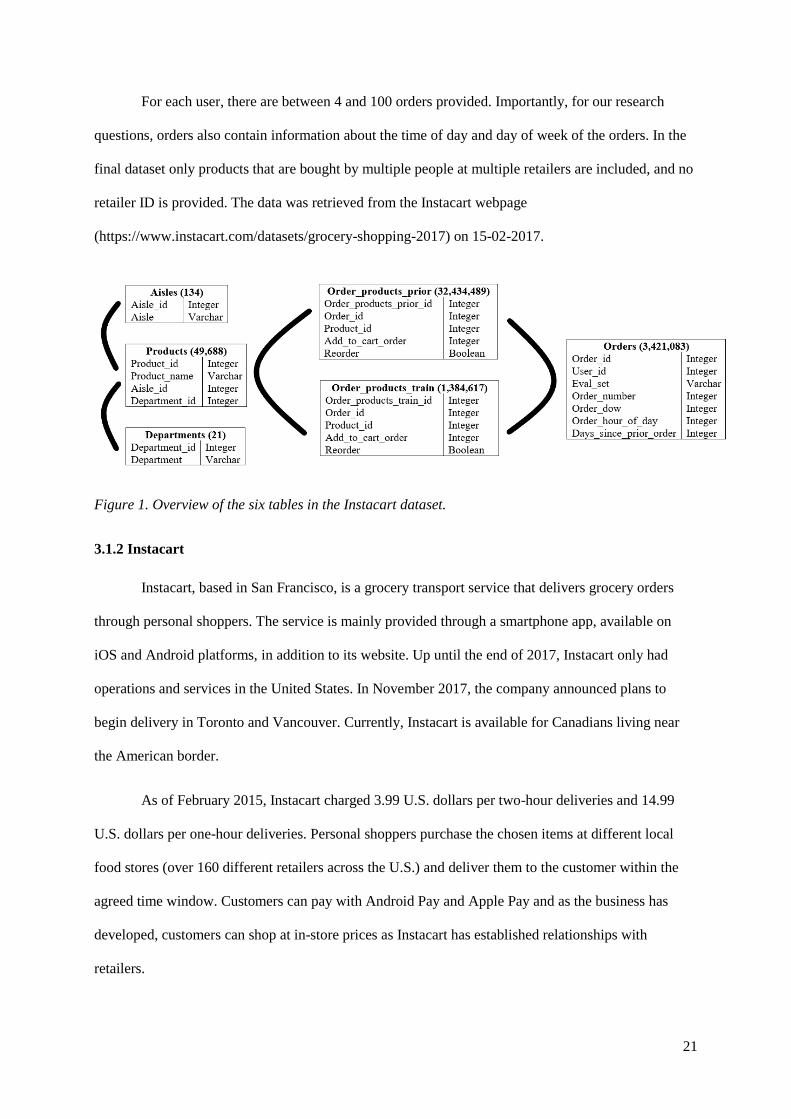
The dataset contains a sample of over 3 million grocery orders from more than 200,000
Instacart users. As shown in Figure 1, it is a linked set of six data tables. At the centre are the products
that were ordered (about 35 million entries), with a product id, order id, and information about the
order in which the items within an order were purchased. Further information about these products is
stored in a separate table containing the product id, producer name, aisle id and department id (about
50 thousand entries). Separate aisle and department tables provide further details about these aspects
of the orders (134 and 21 entries, respectively). Ordered products are grouped into orders (about 3
million entries).
21
For each user, there are between 4 and 100 orders provided. Importantly, for our research
questions, orders also contain information about the time of day and day of week of the orders. In the
final dataset only products that are bought by multiple people at multiple retailers are included, and no
retailer ID is provided. The data was retrieved from the Instacart webpage
(https://www.instacart.com/datasets/grocery-shopping-2017) on 15-02-2017.
Figure 1. Overview of the six tables in the Instacart dataset.
3.1.2 Instacart
Instacart, based in San Francisco, is a grocery transport service that delivers grocery orders
through personal shoppers. The service is mainly provided through a smartphone app, available on
iOS and Android platforms, in addition to its website. Up until the end of 2017, Instacart only had
operations and services in the United States. In November 2017, the company announced plans to
begin delivery in Toronto and Vancouver. Currently, Instacart is available for Canadians living near
the American border.
As of February 2015, Instacart charged 3.99 U.S. dollars per two-hour deliveries and 14.99
U.S. dollars per one-hour deliveries. Personal shoppers purchase the chosen items at different local
food stores (over 160 different retailers across the U.S.) and deliver them to the customer within the
agreed time window. Customers can pay with Android Pay and Apple Pay and as the business has
developed, customers can shop at in-store prices as Instacart has established relationships with
retailers.
22
3.1.3 Programming language
The data was analysed with Python, a general-purpose, open source computer programming
language. In order to use Python for machine learning additional toolkits were required. A toolkit that
was used in this study is scikit-learn, a Python module integrating a wide range of state-of-the-art
machine learning algorithms for medium-scale supervised and unsupervised problems (Pedregosa et
al., 2011). This package focusses on bringing machine learning to non-specialists using a general-
purpose high-level language. Other packages that were used include; SciPy, Pandas, NumPy, Seaborn
and, matplotlib (library for producing plots and other two-dimensional data visualizations)
(McKinney, 2012).
3.2 Pre-processing
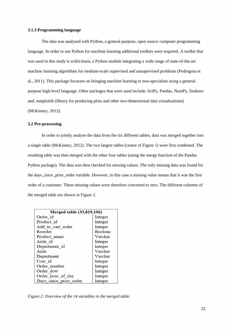
In order to jointly analyse the data from the six different tables, data was merged together into
a single table (McKinney, 2012). The two largest tables (centre of Figure 1) were first combined. The
resulting table was then merged with the other four tables (using the merge function of the Pandas
Python package). The data was then checked for missing values. The only missing data was found for
the days_since_prior_order variable. However, in this case a missing value means that it was the first
order of a customer. These missing values were therefore converted to zero. The different columns of
the merged table are shown in Figure 2.
Figure 2. Overview of the 14 variables in the merged table.
23
The merged table functioned as the base for all further steps. Next, to speed up calculations
some of data types were converted for computation. To demonstrate, integer and float data types were
converted from 64bit to 32bit. Also, object data types were converted to category types. For the first
two research questions, data were aggregated into a single row of data per order_id. That is because
the first two research questions inquire basic information (e.g., time of purchase) of orders and not
about the products of a single order. The resulting table was split into a training (80%) and a test set
(20%) as the Pareto Principle states, as detailed in Section 3.5 (Evaluation criteria).
3.3 Feature engineering
3.3.1 Feature selection
Feature selection, also known as variable selection, is an important step to improve the
performance of the classification techniques. It reduces the dataset by removing irrelevant, redundant,
or noisy features and has a significant effect on speeding up the data mining algorithms, improving the
learning accuracy, and better understanding of a model (Nejad & Abadi, 2014). To reduce memory
allocation unused columns were deleted. These deleted columns were aisle, department, and
product_name (because of these columns being identical to other variables). More features were
deleted for the final prediction, as detailed in Section 3.5 (Evaluation criteria).
3.3.2 Feature construction
Feature construction involves transforming a given set of input features to generate a new set
of more powerful features which can then be used for prediction. This can involve turning a variable
with multiple categories to one with only two categories (dichotomization). The order_dow (day of the
week) variable was recoded into two categories going from seven categories (each day of the week) to
two levels (weekday or weekend). A further advantage was that after recoding, the variable was more
balanced.
To speed up calculations for research questions 1 and 2, which focussed on orders rather than
individual items inside orders, data were aggregated to the order level, removing data about individual
items. Specifically, a new variable was created to code the order size. For the remaining research
questions, some columns with numerical data were turned into binary categories, applying the Python
24
pandas function qcut(). For research question 3, concerning product information, two different tables
were used to explore the data. One with information about orders and one containing information
about individual items inside orders.
Modes were calculated for the order table to represent the most chosen product category of
that order. Therefore, the most common department and aisle of an order were used as product
information. Likewise, the first added product of an order was used as a new variable. Furthermore,
product names were used to determine whether a product was organic or not. Products were marked as
organic if the product name contained the word ‘organic’. Likewise, an order was marked organic if
that order contained at least one organic product. To speed up calculations, modes and organic
products were saved as Excel files and merged to the order table. In this way, computations only had
to be executed once.
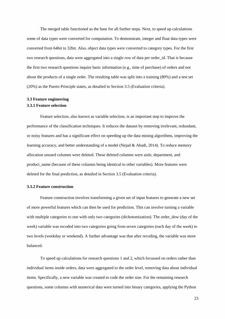
The table containing information about orders was used to answer research question 4; the
prediction of the shopper (weekend or weekday). As shown in Figure 3, the single order table holds
several variables including point of time the order is placed, order size and which user the order
placed.
Figure 3. Table with information about orders
The weekend and weekday variables were constructed to hold information about probabilities
of an order made at the weekend or during weekdays. For instance, in total 100,000 apples were
bought; 15,000 at the weekend and 85,000 during weekdays. The probability that an apple was ordered
25
during a weekday is (85,000 * 100) / 100,000 = 85 percent. Probabilities were calculated for users,
products and combinations of variables. If the probability was higher than eighty percent that a user
placed an order at the weekend or during weekdays then the user was marked with a one and a zero in
the constructed columns week or weekend, depending on the probability of being in one of these
groups. If the probability was eighty percent or lower then the user was marked with a zero in both
columns.
3.4 Experimental procedure
As choices of data mining techniques should be based on the data characteristics and business
requirements (Giraud-Carrier & Povel, 2003), visualizations are used to explore the data, before using
classification to predict customer types. After recoding of the data, the dependent variable of interest,
whether products were ordered on a weekday or weekend, was binary, and therefore classification
methods are the most suitable methods to analyse the data. By constructing a model that predicts the
type of buyer (weekday or weekend), buyer profiles can be constructed, which may help identify the
most profitable and loyal customers, serve each customer according to their specific needs and
preferences, balance demand planning, response and execution. With this intention, classification can
be used to build a model to predict future customer behaviours through classifying database records
into a number of predefined classes based on certain criteria.
Classification is an important data mining technique with broad applications to classify
various kinds of data and is used to classify items according to the features of the item with respect to
the predefined set of classes (Patil et al., 2013). Data classification is a two-step process, consisting of
a learning step (where a classification model is constructed) and a classification step (where the
classification model is used to predict class labels for given data). Classification models can be built
with various classification techniques from an input data set. As multiple studies state that there is no
single technique that works best for every problem (Caruana & Niculescu-Mizil, 2006; Novaković,
2016), multiple classifiers were tried. Three classification techniques were used to predict purchasing
behaviour in this study: decision trees, random forests and artificial neural networks (ANNs). Neural
networks are proficient at giving better classification results by using non-linear boundaries. However,
26
ANNs take more time to train and are slower for classification tasks in comparison with decision trees.
Also, decision trees are very interpretable and ANN’s are not (Buckinx et al., 2005).
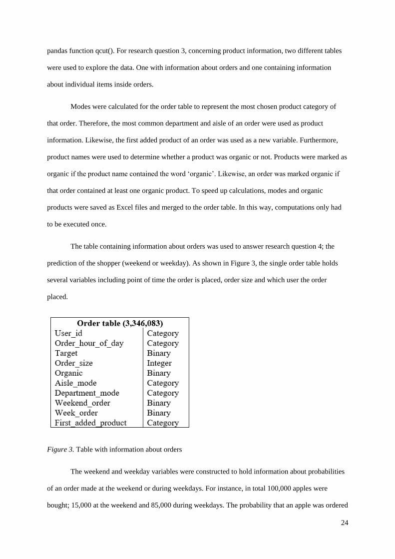
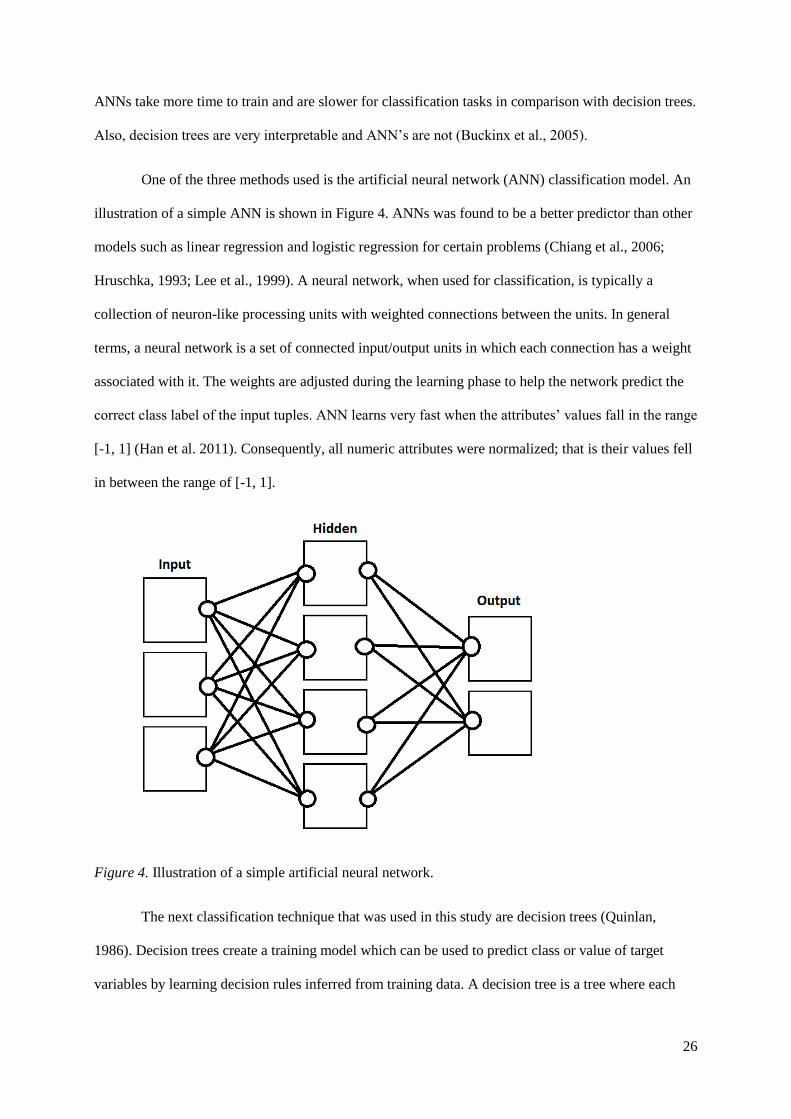
One of the three methods used is the artificial neural network (ANN) classification model. An
illustration of a simple ANN is shown in Figure 4. ANNs was found to be a better predictor than other
models such as linear regression and logistic regression for certain problems (Chiang et al., 2006;
Hruschka, 1993; Lee et al., 1999). A neural network, when used for classification, is typically a
collection of neuron-like processing units with weighted connections between the units. In general
terms, a neural network is a set of connected input/output units in which each connection has a weight
associated with it. The weights are adjusted during the learning phase to help the network predict the
correct class label of the input tuples. ANN learns very fast when the attributes’ values fall in the range
[-1, 1] (Han et al. 2011). Consequently, all numeric attributes were normalized; that is their values fell
in between the range of [-1, 1].
Figure 4. Illustration of a simple artificial neural network.
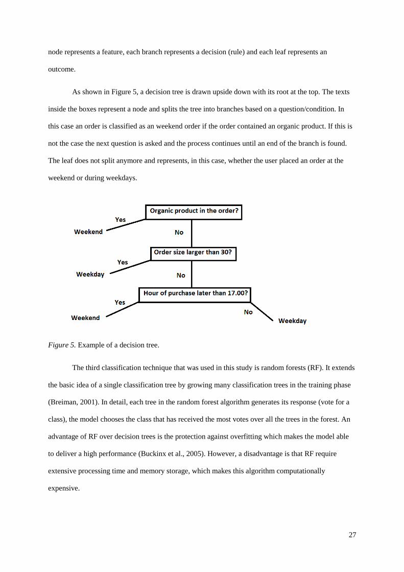
The next classification technique that was used in this study are decision trees (Quinlan,
1986). Decision trees create a training model which can be used to predict class or value of target
variables by learning decision rules inferred from training data. A decision tree is a tree where each
27
node represents a feature, each branch represents a decision (rule) and each leaf represents an
outcome.
As shown in Figure 5, a decision tree is drawn upside down with its root at the top. The texts
inside the boxes represent a node and splits the tree into branches based on a question/condition. In
this case an order is classified as an weekend order if the order contained an organic product. If this is
not the case the next question is asked and the process continues until an end of the branch is found.
The leaf does not split anymore and represents, in this case, whether the user placed an order at the
weekend or during weekdays.
Figure 5. Example of a decision tree.
The third classification technique that was used in this study is random forests (RF). It extends
the basic idea of a single classification tree by growing many classification trees in the training phase
(Breiman, 2001). In detail, each tree in the random forest algorithm generates its response (vote for a
class), the model chooses the class that has received the most votes over all the trees in the forest. An
advantage of RF over decision trees is the protection against overfitting which makes the model able
to deliver a high performance (Buckinx et al., 2005). However, a disadvantage is that RF require
extensive processing time and memory storage, which makes this algorithm computationally
expensive.
28
3.5 Evaluation criteria
Cross-validation was used to compare the algorithms, choose the best features and also to
optimize the parameters of those algorithms. To avoid that the algorithms had seen all data in order to
establish the best model structure (i.e., variables in the model and their weights), a test set was taken
from the dataset before cross-validation, feature selection and model optimization. Subsequently, the
trained algorithm was applied to unseen data. Testing learning algorithms on the same data would lead
to overfitting, a model that would just repeat the labels of the samples that it has just seen would have
a perfect score but would fail to predict anything useful on unseen data. Therefore, hold-out validation
was used, which splits the dataset into two non-overlapped parts: one for training and the other for
testing. The test data was held out and not used during training. This method avoids the overlap
between training data and test data, yielding a more accurate estimate for the generalization
performance of the algorithm.
The best features for the final prediction were selected using principal component analysis
(PCA), non-negative matrix factorization (NMF or NNMF) and univariate feature selection in
combination with k-fold cross-validation. Four features achieved the highest accuracy for all three
feature selection algorithms; first_added_product, weekend_order, week_order and user_id. Those
four features were kept in the table for final prediction.
The parameters of the algorithms were optimized using random experiments in combination
with k-fold cross-validation, which is the basic form of cross-validation. Random search found to be
more efficient and less time consuming than grid search for hyper-parameter optimization because not
all hyperparameters are equally important to tune (Bergstra & Bengio, 2012). Grid search is the
process of scanning the data to construct optimal parameters for a given model. It will build a model
on each parameter combination possible, iterates through every parameter combination, and stores a
model for each combination. Random search is a direct search method as it does not require
derivatives to search a continuous domain. As a standard computer was found to struggle to perform
the relevant parameter optimization on the entire training set, these analyses were performed on a
subset of the training set.

29
Next, the training data was first partitioned into equally sized segments/folds. A sufficient
number of folds would reduce the chance of overfitting but would also increase computation time per
fold. Provided that, three folds were used as the data table was large. K iterations of training and
validation were performed such that within each iteration a different fold of the data is held-out for
validation while the remaining k-1 folds are used for learning. In each iteration, the algorithm with one
or more parameter combinations used k-1 folds of data to learn one or more models, and subsequently
the learned models are asked to make predictions about the data in the validation fold. The
performance of each parameter combination on each fold was tracked by accuracy. Eventually, the
best combinations for each algorithm were kept.
After each classifier was adjusted and best parameters were chosen the different learning
algorithms had to be compared. This task was performed on the training set and the evaluation of the
final model was done on the test set. In order to tell whether the different algorithms delivered good
results, a baseline model was used for comparison. The most common class prediction was chosen as a
baseline model for comparison with the algorithms. This means that, for this dataset, the baseline
model will predict that all instances are weekday instances as most orders were ordered during
weekdays.
The performance of classification algorithms was examined by evaluating the accuracy or
error rate of the classification. Accuracy is usually calculated by determining the percentage of tuples
placed in a correct class. However, this ignores the fact that there may also be a cost associated with an
incorrect assignment to the wrong class (Patil et al., 2013). Therefore, the results of the classifier were
tested using true positives, true negatives, false positives, and false negatives. The terms positive and
negative refer to the classifier's prediction, and the terms true and false refer to whether that prediction
corresponds to the external judgment. Incorrect and correct classifications were described in a
confusion matrix.
A confusion matrix illustrates the accuracy of the solution to a classification problem and
contains information about actual and predicted classifications. The classifications are true positive
30
(TP) if the outcome from a prediction is p and the actual value is also p. A classification is false
positive (FP) if the outcome from a prediction is p but the actual value is n.
Performance was also measured with recall (the true positive rate or sensitivity) and precision
(positive predictive value). Precision is the fraction of retrieved instances that are relevant, while recall
is defined as the number of true positives divided by the total number of elements that actually belong
to the positive class. However, a hundred percent recall can be achieved while precision is very poor.
Therefore, precision and recall were combined into f-measure, a single measure of overall
performance (Manning & Schütze, 1999).
4 Results
The aim of this research was to investigate whether weekday and weekend online shoppers
differ. Three research questions focus on investigating differences in terms of ordering times, order size
and types of products. The fourth research question aims at predicting the type of shopper (weekend or
weekday). Therefore, three classification algorithms were used; decision tree, random forest, and neural
network.
4.1 Ordering time
To address the first research question, whether weekday shoppers order at different times than
weekend shoppers, ordering times of orders were analysed. The dataset used contained a total of
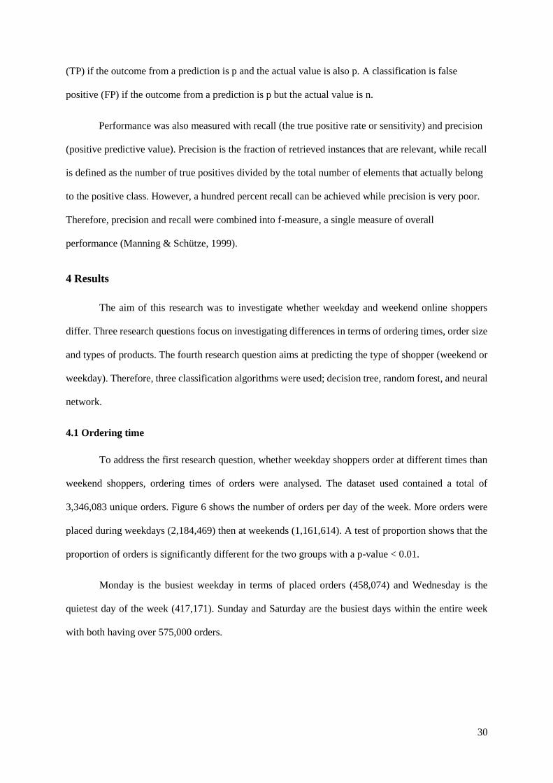
3,346,083 unique orders. Figure 6 shows the number of orders per day of the week. More orders were
placed during weekdays (2,184,469) then at weekends (1,161,614). A test of proportion shows that the
proportion of orders is significantly different for the two groups with a p-value < 0.01.
Monday is the busiest weekday in terms of placed orders (458,074) and Wednesday is the
quietest day of the week (417,171). Sunday and Saturday are the busiest days within the entire week
with both having over 575,000 orders.
31
Figure 6. Histogram of total orders distributed by day of the week.
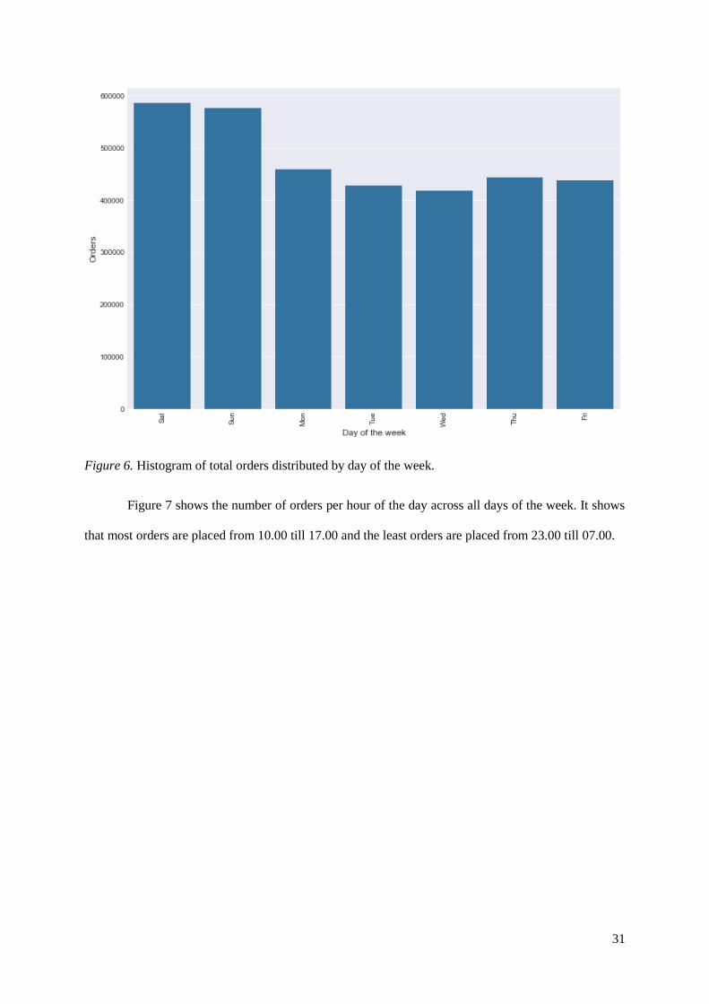
Figure 7 shows the number of orders per hour of the day across all days of the week. It shows
that most orders are placed from 10.00 till 17.00 and the least orders are placed from 23.00 till 07.00.
32
Figure 7. Histogram of total orders distributed by hour of the day
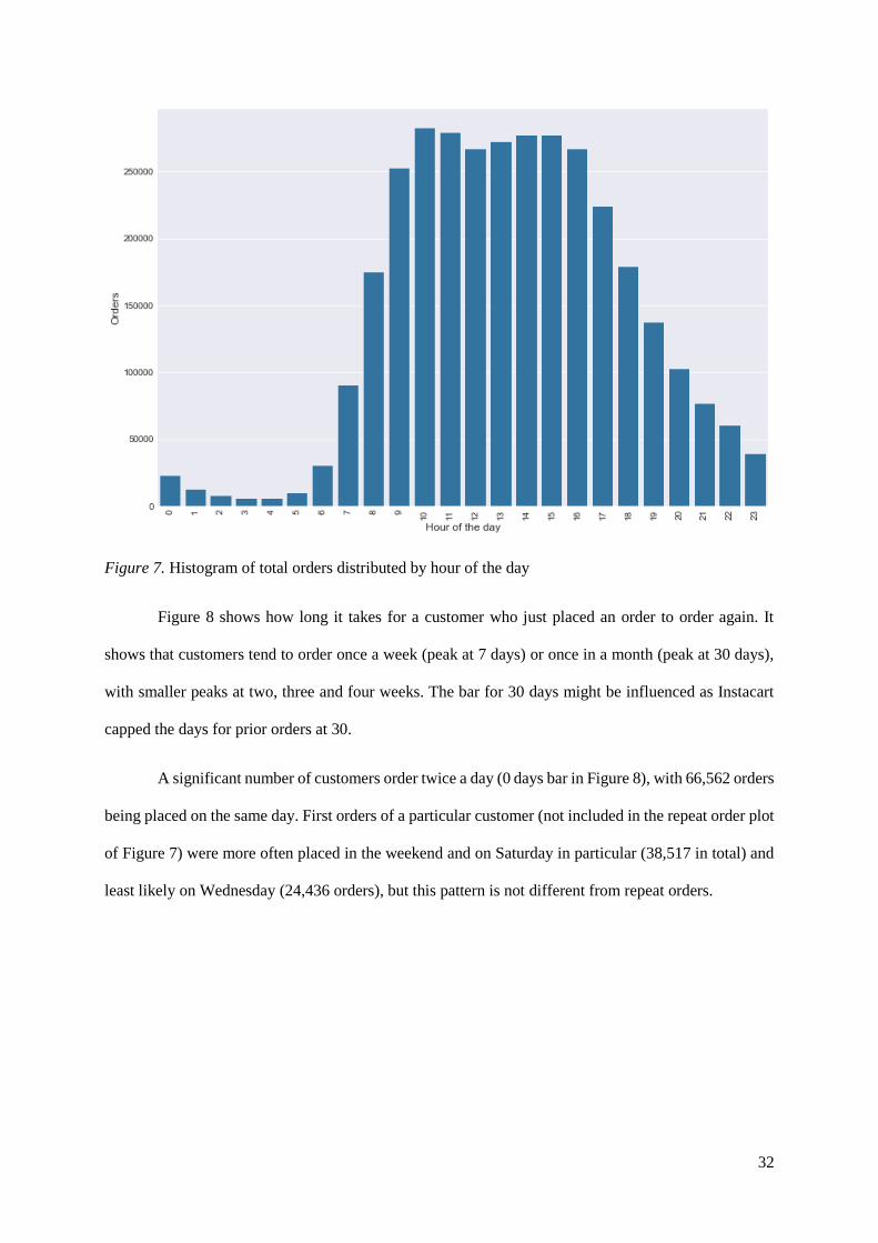
Figure 8 shows how long it takes for a customer who just placed an order to order again. It
shows that customers tend to order once a week (peak at 7 days) or once in a month (peak at 30 days),
with smaller peaks at two, three and four weeks. The bar for 30 days might be influenced as Instacart
capped the days for prior orders at 30.
A significant number of customers order twice a day (0 days bar in Figure 8), with 66,562 orders
being placed on the same day. First orders of a particular customer (not included in the repeat order plot
of Figure 7) were more often placed in the weekend and on Saturday in particular (38,517 in total) and
least likely on Wednesday (24,436 orders), but this pattern is not different from repeat orders.
33
Figure 8. Histogram of total orders distributed by days since prior order.
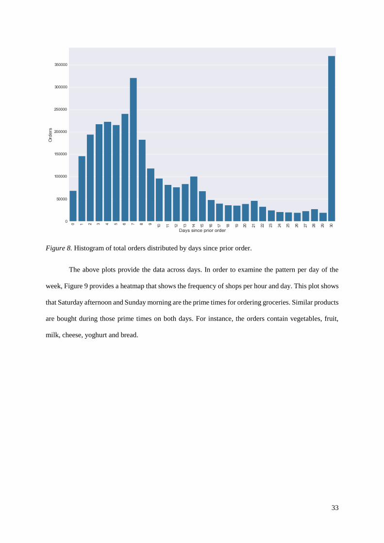
The above plots provide the data across days. In order to examine the pattern per day of the
week, Figure 9 provides a heatmap that shows the frequency of shops per hour and day. This plot shows
that Saturday afternoon and Sunday morning are the prime times for ordering groceries. Similar products
are bought during those prime times on both days. For instance, the orders contain vegetables, fruit,
milk, cheese, yoghurt and bread.
34
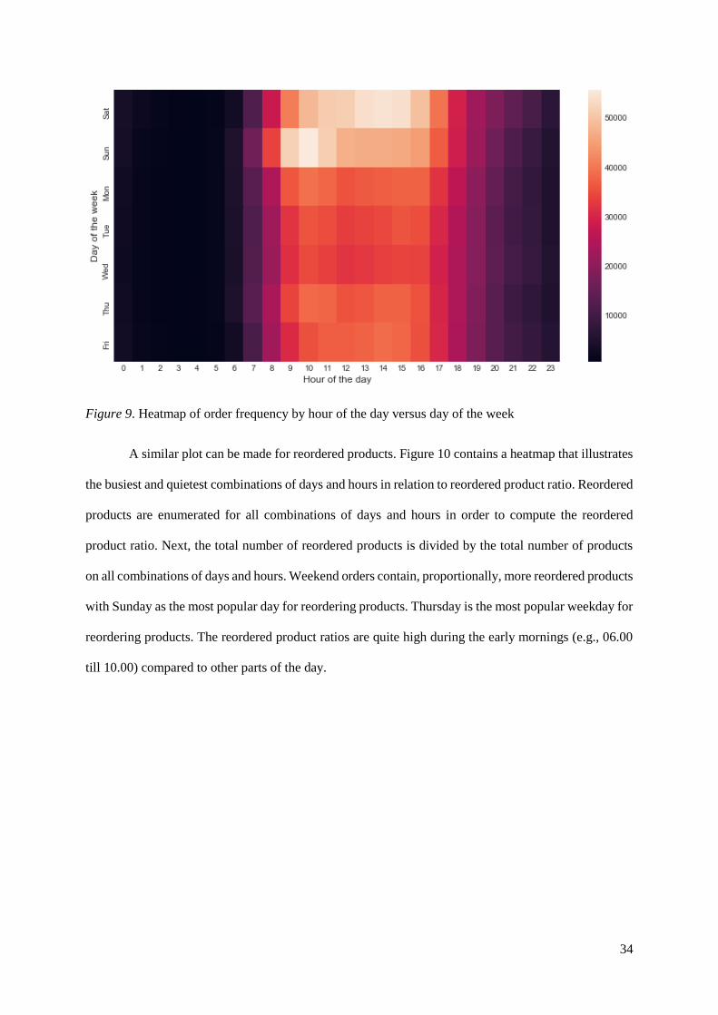
Figure 9. Heatmap of order frequency by hour of the day versus day of the week
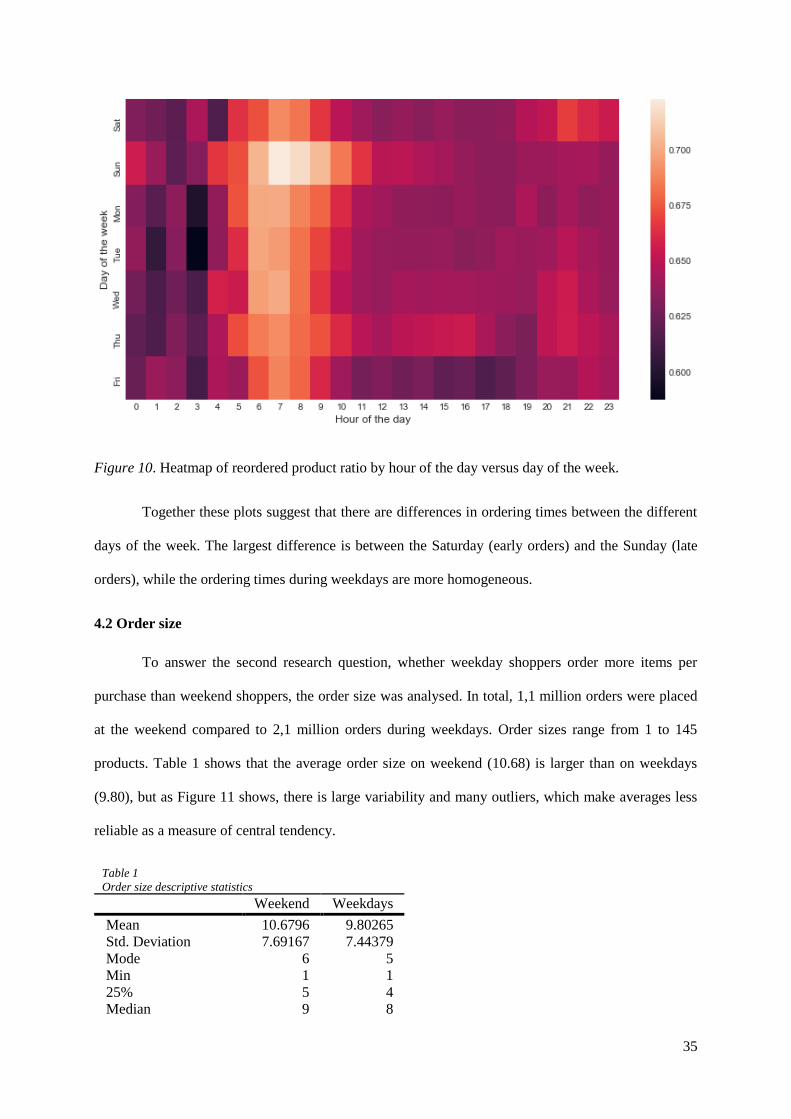
A similar plot can be made for reordered products. Figure 10 contains a heatmap that illustrates
the busiest and quietest combinations of days and hours in relation to reordered product ratio. Reordered
products are enumerated for all combinations of days and hours in order to compute the reordered
product ratio. Next, the total number of reordered products is divided by the total number of products
on all combinations of days and hours. Weekend orders contain, proportionally, more reordered products
with Sunday as the most popular day for reordering products. Thursday is the most popular weekday for
reordering products. The reordered product ratios are quite high during the early mornings (e.g., 06.00
till 10.00) compared to other parts of the day.
35
Figure 10. Heatmap of reordered product ratio by hour of the day versus day of the week.
Together these plots suggest that there are differences in ordering times between the different
days of the week. The largest difference is between the Saturday (early orders) and the Sunday (late
orders), while the ordering times during weekdays are more homogeneous.
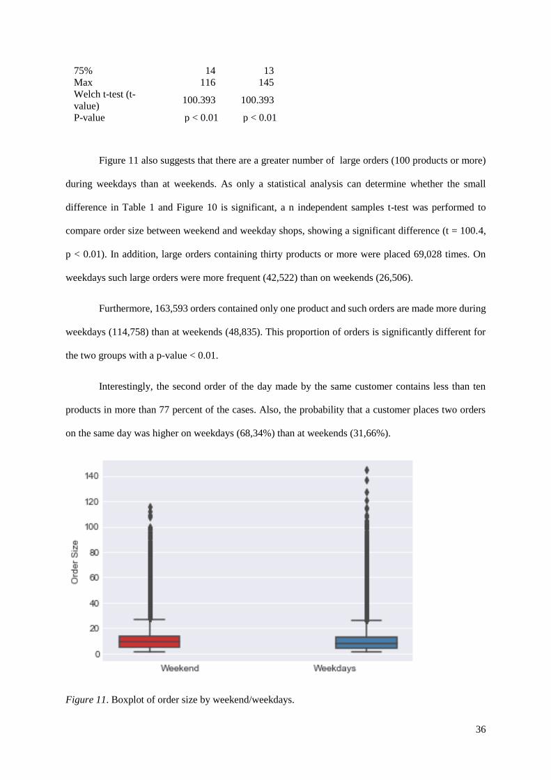
4.2 Order size
To answer the second research question, whether weekday shoppers order more items per
purchase than weekend shoppers, the order size was analysed. In total, 1,1 million orders were placed
at the weekend compared to 2,1 million orders during weekdays. Order sizes range from 1 to 145
products. Table 1 shows that the average order size on weekend (10.68) is larger than on weekdays
(9.80), but as Figure 11 shows, there is large variability and many outliers, which make averages less
reliable as a measure of central tendency.
Table 1 Order size descriptive statistics
Weekend Weekdays
Mean 10.6796 9.80265 Std. Deviation 7.69167 7.44379 Mode 6 5 Min 1 1 25% 5 4 Median 9 8
36
75% 14 13 Max 116 145 Welch t-test (t-
value) 100.393 100.393
P-value p < 0.01 p < 0.01
Figure 11 also suggests that there are a greater number of large orders (100 products or more)
during weekdays than at weekends. As only a statistical analysis can determine whether the small
difference in Table 1 and Figure 10 is significant, a n independent samples t-test was performed to
compare order size between weekend and weekday shops, showing a significant difference (t = 100.4,
p < 0.01). In addition, large orders containing thirty products or more were placed 69,028 times. On
weekdays such large orders were more frequent (42,522) than on weekends (26,506).
Furthermore, 163,593 orders contained only one product and such orders are made more during
weekdays (114,758) than at weekends (48,835). This proportion of orders is significantly different for
the two groups with a p-value < 0.01.
Interestingly, the second order of the day made by the same customer contains less than ten
products in more than 77 percent of the cases. Also, the probability that a customer places two orders
on the same day was higher on weekdays (68,34%) than at weekends (31,66%).
Figure 11. Boxplot of order size by weekend/weekdays.
37
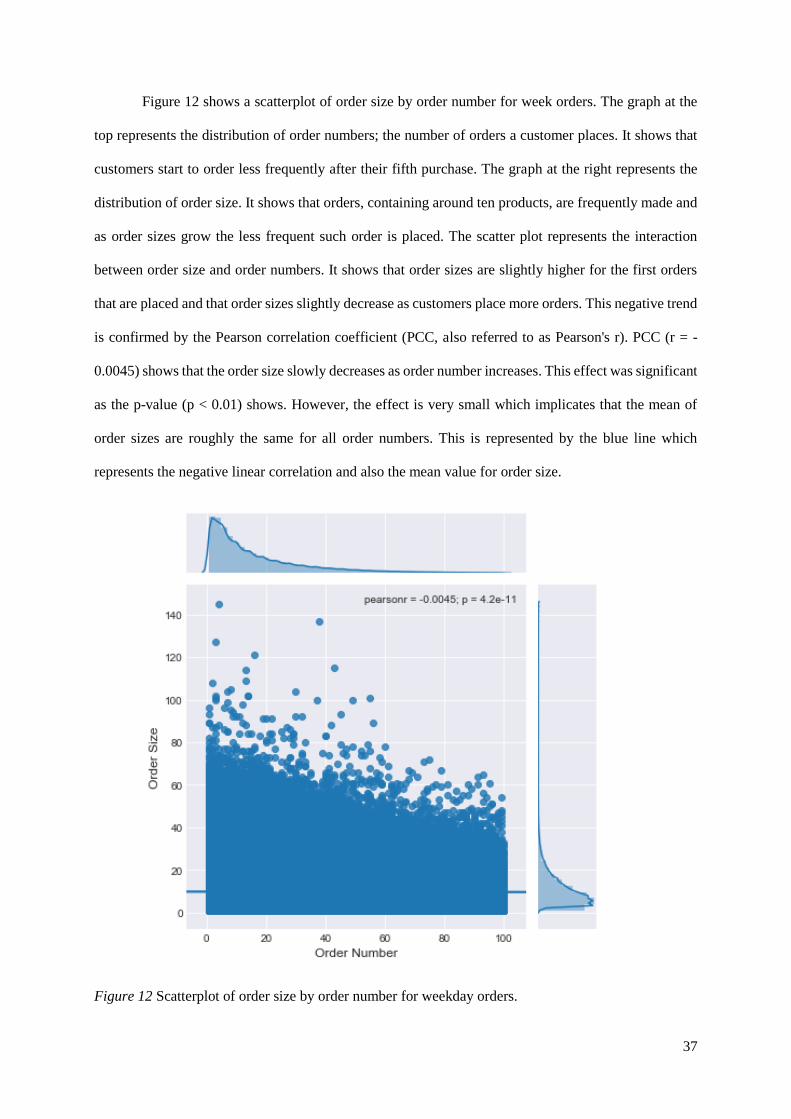
Figure 12 shows a scatterplot of order size by order number for week orders. The graph at the
top represents the distribution of order numbers; the number of orders a customer places. It shows that
customers start to order less frequently after their fifth purchase. The graph at the right represents the
distribution of order size. It shows that orders, containing around ten products, are frequently made and
as order sizes grow the less frequent such order is placed. The scatter plot represents the interaction
between order size and order numbers. It shows that order sizes are slightly higher for the first orders
that are placed and that order sizes slightly decrease as customers place more orders. This negative trend
is confirmed by the Pearson correlation coefficient (PCC, also referred to as Pearson's r). PCC (r = -
0.0045) shows that the order size slowly decreases as order number increases. This effect was significant
as the p-value (p < 0.01) shows. However, the effect is very small which implicates that the mean of
order sizes are roughly the same for all order numbers. This is represented by the blue line which
represents the negative linear correlation and also the mean value for order size.
Figure 12 Scatterplot of order size by order number for weekday orders.
38
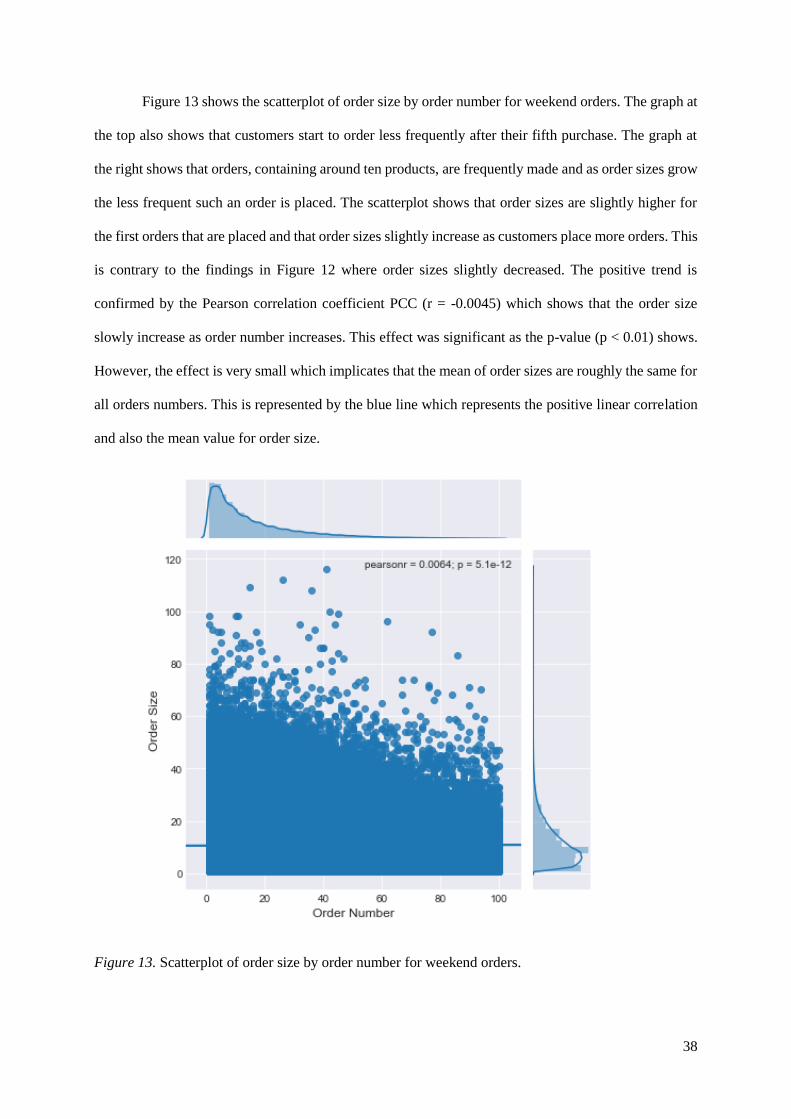
Figure 13 shows the scatterplot of order size by order number for weekend orders. The graph at
the top also shows that customers start to order less frequently after their fifth purchase. The graph at
the right shows that orders, containing around ten products, are frequently made and as order sizes grow
the less frequent such an order is placed. The scatterplot shows that order sizes are slightly higher for
the first orders that are placed and that order sizes slightly increase as customers place more orders. This
is contrary to the findings in Figure 12 where order sizes slightly decreased. The positive trend is
confirmed by the Pearson correlation coefficient PCC (r = -0.0045) which shows that the order size
slowly increase as order number increases. This effect was significant as the p-value (p < 0.01) shows.
However, the effect is very small which implicates that the mean of order sizes are roughly the same for
all orders numbers. This is represented by the blue line which represents the positive linear correlation
and also the mean value for order size.
Figure 13. Scatterplot of order size by order number for weekend orders.
39
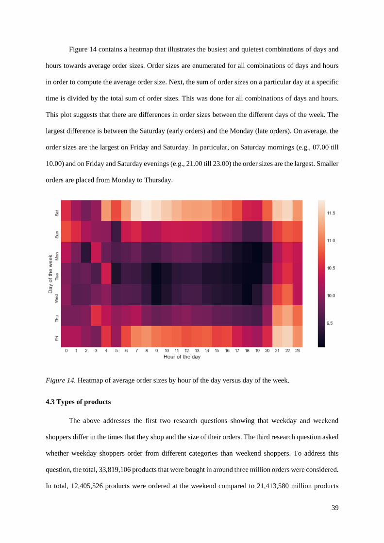
Figure 14 contains a heatmap that illustrates the busiest and quietest combinations of days and
hours towards average order sizes. Order sizes are enumerated for all combinations of days and hours
in order to compute the average order size. Next, the sum of order sizes on a particular day at a specific
time is divided by the total sum of order sizes. This was done for all combinations of days and hours.
This plot suggests that there are differences in order sizes between the different days of the week. The
largest difference is between the Saturday (early orders) and the Monday (late orders). On average, the
order sizes are the largest on Friday and Saturday. In particular, on Saturday mornings (e.g., 07.00 till
10.00) and on Friday and Saturday evenings (e.g., 21.00 till 23.00) the order sizes are the largest. Smaller
orders are placed from Monday to Thursday.
Figure 14. Heatmap of average order sizes by hour of the day versus day of the week.
4.3 Types of products
The above addresses the first two research questions showing that weekday and weekend
shoppers differ in the times that they shop and the size of their orders. The third research question asked
whether weekday shoppers order from different categories than weekend shoppers. To address this
question, the total, 33,819,106 products that were bought in around three million orders were considered.
In total, 12,405,526 products were ordered at the weekend compared to 21,413,580 million products
40
during weekdays. This proportion of ordered products is significantly different for the two groups with
a p-value < 0.01. There are 49,688 unique products and as a first indicator, the top ten most ordered
products, aisles, and departments were extracted.
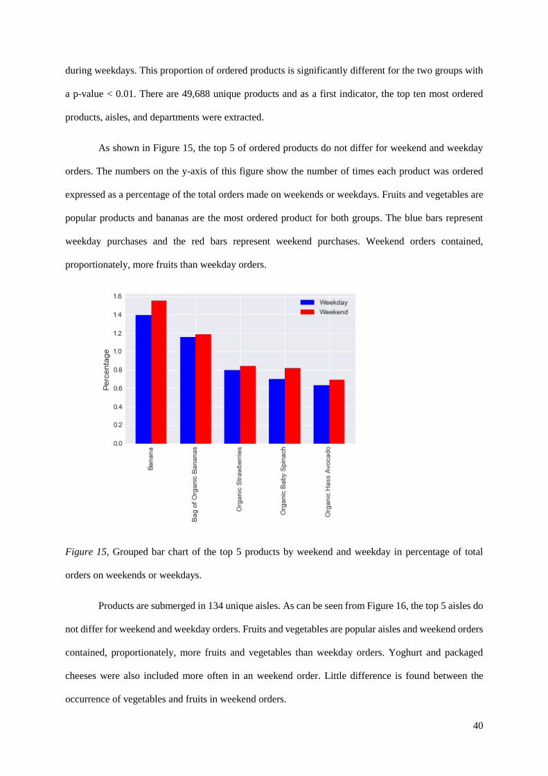
As shown in Figure 15, the top 5 of ordered products do not differ for weekend and weekday
orders. The numbers on the y-axis of this figure show the number of times each product was ordered
expressed as a percentage of the total orders made on weekends or weekdays. Fruits and vegetables are
popular products and bananas are the most ordered product for both groups. The blue bars represent
weekday purchases and the red bars represent weekend purchases. Weekend orders contained,
proportionately, more fruits than weekday orders.
Figure 15, Grouped bar chart of the top 5 products by weekend and weekday in percentage of total
orders on weekends or weekdays.
Products are submerged in 134 unique aisles. As can be seen from Figure 16, the top 5 aisles do
not differ for weekend and weekday orders. Fruits and vegetables are popular aisles and weekend orders
contained, proportionately, more fruits and vegetables than weekday orders. Yoghurt and packaged
cheeses were also included more often in an weekend order. Little difference is found between the
occurrence of vegetables and fruits in weekend orders.
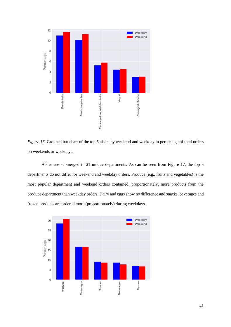
41
Figure 16, Grouped bar chart of the top 5 aisles by weekend and weekday in percentage of total orders
on weekends or weekdays.
Aisles are submerged in 21 unique departments. As can be seen from Figure 17, the top 5
departments do not differ for weekend and weekday orders. Produce (e.g., fruits and vegetables) is the
most popular department and weekend orders contained, proportionately, more products from the
produce department than weekday orders. Dairy and eggs show no difference and snacks, beverages and
frozen products are ordered more (proportionately) during weekdays.
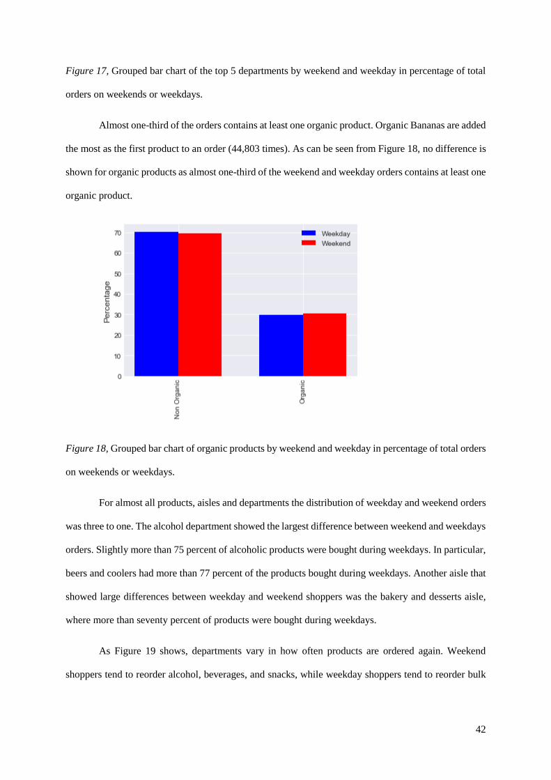
42
Figure 17, Grouped bar chart of the top 5 departments by weekend and weekday in percentage of total
orders on weekends or weekdays.
Almost one-third of the orders contains at least one organic product. Organic Bananas are added
the most as the first product to an order (44,803 times). As can be seen from Figure 18, no difference is
shown for organic products as almost one-third of the weekend and weekday orders contains at least one
organic product.
Figure 18, Grouped bar chart of organic products by weekend and weekday in percentage of total orders
on weekends or weekdays.
For almost all products, aisles and departments the distribution of weekday and weekend orders
was three to one. The alcohol department showed the largest difference between weekend and weekdays
orders. Slightly more than 75 percent of alcoholic products were bought during weekdays. In particular,
beers and coolers had more than 77 percent of the products bought during weekdays. Another aisle that
showed large differences between weekday and weekend shoppers was the bakery and desserts aisle,
where more than seventy percent of products were bought during weekdays.
As Figure 19 shows, departments vary in how often products are ordered again. Weekend
shoppers tend to reorder alcohol, beverages, and snacks, while weekday shoppers tend to reorder bulk
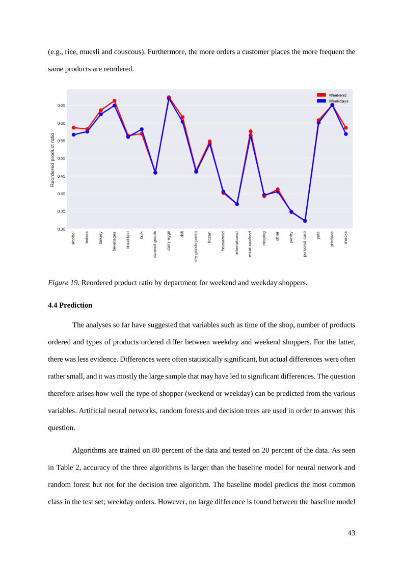
43
(e.g., rice, muesli and couscous). Furthermore, the more orders a customer places the more frequent the
same products are reordered.
Figure 19. Reordered product ratio by department for weekend and weekday shoppers.
4.4 Prediction
The analyses so far have suggested that variables such as time of the shop, number of products
ordered and types of products ordered differ between weekday and weekend shoppers. For the latter,
there was less evidence. Differences were often statistically significant, but actual differences were often
rather small, and it was mostly the large sample that may have led to significant differences. The question
therefore arises how well the type of shopper (weekend or weekday) can be predicted from the various
variables. Artificial neural networks, random forests and decision trees are used in order to answer this
question.
Algorithms are trained on 80 percent of the data and tested on 20 percent of the data. As seen
in Table 2, accuracy of the three algorithms is larger than the baseline model for neural network and
random forest but not for the decision tree algorithm. The baseline model predicts the most common
class in the test set; weekday orders. However, no large difference is found between the baseline model
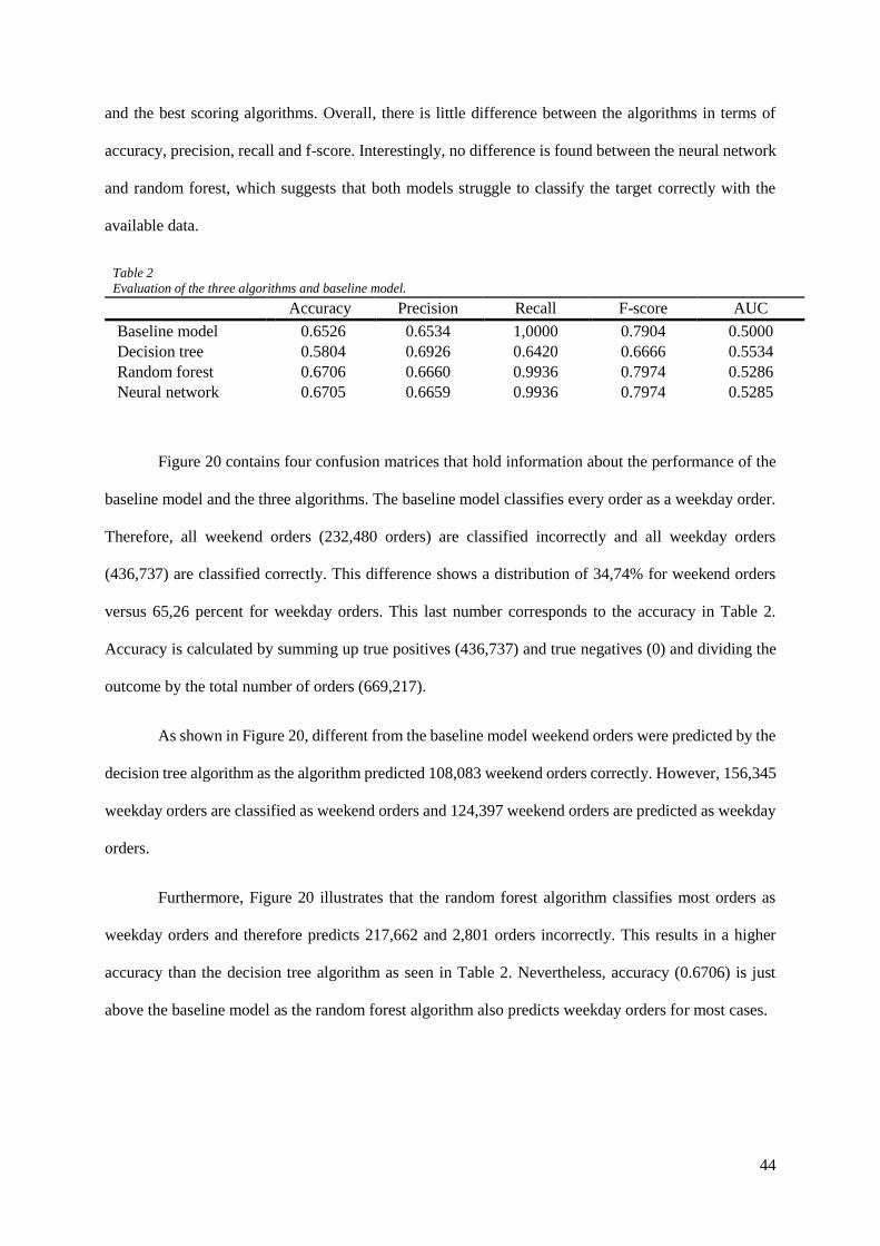
44
and the best scoring algorithms. Overall, there is little difference between the algorithms in terms of
accuracy, precision, recall and f-score. Interestingly, no difference is found between the neural network
and random forest, which suggests that both models struggle to classify the target correctly with the
available data.
Table 2 Evaluation of the three algorithms and baseline model.
Accuracy Precision Recall F-score AUC
Baseline model 0.6526 0.6534 1,0000 0.7904 0.5000
Decision tree 0.5804 0.6926 0.6420 0.6666 0.5534
Random forest 0.6706 0.6660 0.9936 0.7974 0.5286
Neural network 0.6705 0.6659 0.9936 0.7974 0.5285
Figure 20 contains four confusion matrices that hold information about the performance of the
baseline model and the three algorithms. The baseline model classifies every order as a weekday order.
Therefore, all weekend orders (232,480 orders) are classified incorrectly and all weekday orders
(436,737) are classified correctly. This difference shows a distribution of 34,74% for weekend orders
versus 65,26 percent for weekday orders. This last number corresponds to the accuracy in Table 2.
Accuracy is calculated by summing up true positives (436,737) and true negatives (0) and dividing the
outcome by the total number of orders (669,217).
As shown in Figure 20, different from the baseline model weekend orders were predicted by the
decision tree algorithm as the algorithm predicted 108,083 weekend orders correctly. However, 156,345
weekday orders are classified as weekend orders and 124,397 weekend orders are predicted as weekday
orders.
Furthermore, Figure 20 illustrates that the random forest algorithm classifies most orders as
weekday orders and therefore predicts 217,662 and 2,801 orders incorrectly. This results in a higher
accuracy than the decision tree algorithm as seen in Table 2. Nevertheless, accuracy (0.6706) is just
above the baseline model as the random forest algorithm also predicts weekday orders for most cases.
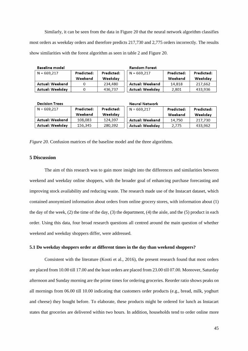
45
Similarly, it can be seen from the data in Figure 20 that the neural network algorithm classifies
most orders as weekday orders and therefore predicts 217,730 and 2,775 orders incorrectly. The results
show similarities with the forest algorithm as seen in table 2 and Figure 20.
Figure 20. Confusion matrices of the baseline model and the three algorithms.
5 Discussion
The aim of this research was to gain more insight into the differences and similarities between
weekend and weekday online shoppers, with the broader goal of enhancing purchase forecasting and
improving stock availability and reducing waste. The research made use of the Instacart dataset, which
contained anonymized information about orders from online grocery stores, with information about (1)
the day of the week, (2) the time of the day, (3) the department, (4) the aisle, and the (5) product in each
order. Using this data, four broad research questions all centred around the main question of whether
weekend and weekday shoppers differ, were addressed.
5.1 Do weekday shoppers order at different times in the day than weekend shoppers?
Consistent with the literature (Kooti et al., 2016), the present research found that most orders
are placed from 10.00 till 17.00 and the least orders are placed from 23.00 till 07.00. Moreover, Saturday
afternoon and Sunday morning are the prime times for ordering groceries. Reorder ratio shows peaks on
all mornings from 06.00 till 10.00 indicating that customers order products (e.g., bread, milk, yoghurt
and cheese) they bought before. To elaborate, these products might be ordered for lunch as Instacart
states that groceries are delivered within two hours. In addition, households tend to order online more
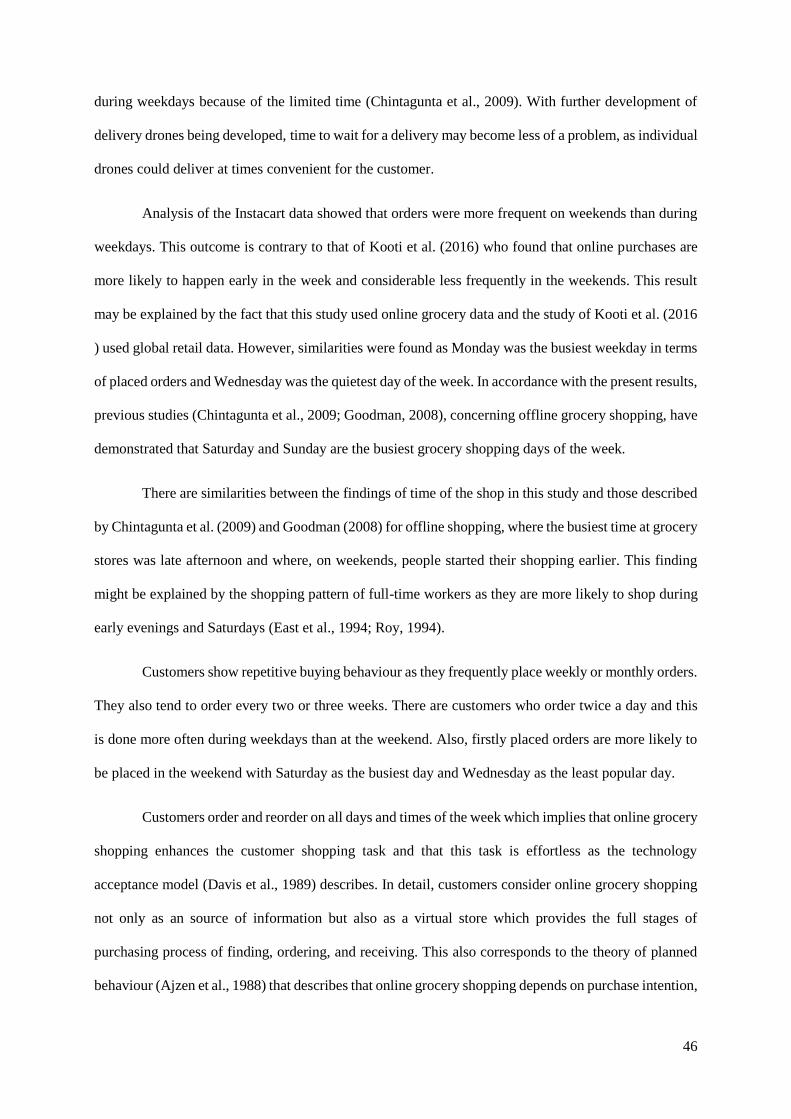
46
during weekdays because of the limited time (Chintagunta et al., 2009). With further development of
delivery drones being developed, time to wait for a delivery may become less of a problem, as individual
drones could deliver at times convenient for the customer.
Analysis of the Instacart data showed that orders were more frequent on weekends than during
weekdays. This outcome is contrary to that of Kooti et al. (2016) who found that online purchases are
more likely to happen early in the week and considerable less frequently in the weekends. This result
may be explained by the fact that this study used online grocery data and the study of Kooti et al. (2016
) used global retail data. However, similarities were found as Monday was the busiest weekday in terms
of placed orders and Wednesday was the quietest day of the week. In accordance with the present results,
previous studies (Chintagunta et al., 2009; Goodman, 2008), concerning offline grocery shopping, have
demonstrated that Saturday and Sunday are the busiest grocery shopping days of the week.
There are similarities between the findings of time of the shop in this study and those described
by Chintagunta et al. (2009) and Goodman (2008) for offline shopping, where the busiest time at grocery
stores was late afternoon and where, on weekends, people started their shopping earlier. This finding
might be explained by the shopping pattern of full-time workers as they are more likely to shop during
early evenings and Saturdays (East et al., 1994; Roy, 1994).
Customers show repetitive buying behaviour as they frequently place weekly or monthly orders.
They also tend to order every two or three weeks. There are customers who order twice a day and this
is done more often during weekdays than at the weekend. Also, firstly placed orders are more likely to
be placed in the weekend with Saturday as the busiest day and Wednesday as the least popular day.
Customers order and reorder on all days and times of the week which implies that online grocery
shopping enhances the customer shopping task and that this task is effortless as the technology
acceptance model (Davis et al., 1989) describes. In detail, customers consider online grocery shopping
not only as an source of information but also as a virtual store which provides the full stages of
purchasing process of finding, ordering, and receiving. This also corresponds to the theory of planned
behaviour (Ajzen et al., 1988) that describes that online grocery shopping depends on purchase intention,
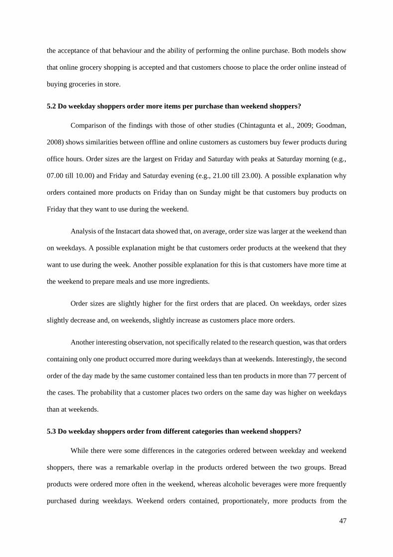
47
the acceptance of that behaviour and the ability of performing the online purchase. Both models show
that online grocery shopping is accepted and that customers choose to place the order online instead of
buying groceries in store.
5.2 Do weekday shoppers order more items per purchase than weekend shoppers?
Comparison of the findings with those of other studies (Chintagunta et al., 2009; Goodman,
2008) shows similarities between offline and online customers as customers buy fewer products during
office hours. Order sizes are the largest on Friday and Saturday with peaks at Saturday morning (e.g.,
07.00 till 10.00) and Friday and Saturday evening (e.g., 21.00 till 23.00). A possible explanation why
orders contained more products on Friday than on Sunday might be that customers buy products on
Friday that they want to use during the weekend.
Analysis of the Instacart data showed that, on average, order size was larger at the weekend than
on weekdays. A possible explanation might be that customers order products at the weekend that they
want to use during the week. Another possible explanation for this is that customers have more time at
the weekend to prepare meals and use more ingredients.
Order sizes are slightly higher for the first orders that are placed. On weekdays, order sizes
slightly decrease and, on weekends, slightly increase as customers place more orders.
Another interesting observation, not specifically related to the research question, was that orders
containing only one product occurred more during weekdays than at weekends. Interestingly, the second
order of the day made by the same customer contained less than ten products in more than 77 percent of
the cases. The probability that a customer places two orders on the same day was higher on weekdays
than at weekends.
5.3 Do weekday shoppers order from different categories than weekend shoppers?
While there were some differences in the categories ordered between weekday and weekend
shoppers, there was a remarkable overlap in the products ordered between the two groups. Bread
products were ordered more often in the weekend, whereas alcoholic beverages were more frequently
purchased during weekdays. Weekend orders contained, proportionately, more products from the
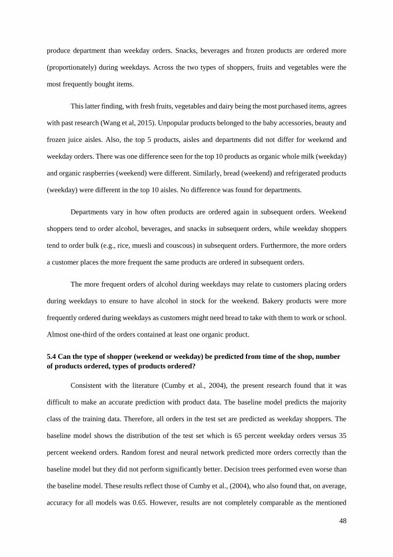
48
produce department than weekday orders. Snacks, beverages and frozen products are ordered more
(proportionately) during weekdays. Across the two types of shoppers, fruits and vegetables were the
most frequently bought items.
This latter finding, with fresh fruits, vegetables and dairy being the most purchased items, agrees
with past research (Wang et al, 2015). Unpopular products belonged to the baby accessories, beauty and
frozen juice aisles. Also, the top 5 products, aisles and departments did not differ for weekend and
weekday orders. There was one difference seen for the top 10 products as organic whole milk (weekday)
and organic raspberries (weekend) were different. Similarly, bread (weekend) and refrigerated products
(weekday) were different in the top 10 aisles. No difference was found for departments.
Departments vary in how often products are ordered again in subsequent orders. Weekend
shoppers tend to order alcohol, beverages, and snacks in subsequent orders, while weekday shoppers
tend to order bulk (e.g., rice, muesli and couscous) in subsequent orders. Furthermore, the more orders
a customer places the more frequent the same products are ordered in subsequent orders.
The more frequent orders of alcohol during weekdays may relate to customers placing orders
during weekdays to ensure to have alcohol in stock for the weekend. Bakery products were more
frequently ordered during weekdays as customers might need bread to take with them to work or school.
Almost one-third of the orders contained at least one organic product.
5.4 Can the type of shopper (weekend or weekday) be predicted from time of the shop, number
of products ordered, types of products ordered?
Consistent with the literature (Cumby et al., 2004), the present research found that it was
difficult to make an accurate prediction with product data. The baseline model predicts the majority
class of the training data. Therefore, all orders in the test set are predicted as weekday shoppers. The
baseline model shows the distribution of the test set which is 65 percent weekday orders versus 35
percent weekend orders. Random forest and neural network predicted more orders correctly than the
baseline model but they did not perform significantly better. Decision trees performed even worse than
the baseline model. These results reflect those of Cumby et al., (2004), who also found that, on average,
accuracy for all models was 0.65. However, results are not completely comparable as the mentioned
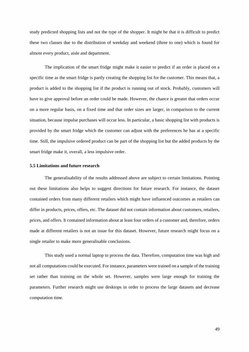
49
study predicted shopping lists and not the type of the shopper. It might be that it is difficult to predict
these two classes due to the distribution of weekday and weekend (three to one) which is found for
almost every product, aisle and department.
The implication of the smart fridge might make it easier to predict if an order is placed on a
specific time as the smart fridge is partly creating the shopping list for the customer. This means that, a
product is added to the shopping list if the product is running out of stock. Probably, customers will
have to give approval before an order could be made. However, the chance is greater that orders occur
on a more regular basis, on a fixed time and that order sizes are larger, in comparison to the current
situation, because impulse purchases will occur less. In particular, a basic shopping list with products is
provided by the smart fridge which the customer can adjust with the preferences he has at a specific
time. Still, the impulsive ordered product can be part of the shopping list but the added products by the
smart fridge make it, overall, a less impulsive order.
5.5 Limitations and future research
The generalisability of the results addressed above are subject to certain limitations. Pointing
out these limitations also helps to suggest directions for future research. For instance, the dataset
contained orders from many different retailers which might have influenced outcomes as retailers can
differ in products, prices, offers, etc. The dataset did not contain information about customers, retailers,
prices, and offers. It contained information about at least four orders of a customer and, therefore, orders
made at different retailers is not an issue for this dataset. However, future research might focus on a
single retailer to make more generalisable conclusions.
This study used a normal laptop to process the data. Therefore, computation time was high and
not all computations could be executed. For instance, parameters were trained on a sample of the training
set rather than training on the whole set. However, samples were large enough for training the
parameters. Further research might use desktops in order to process the large datasets and decrease
computation time.
50
As the dataset did not contain demographic features, future research might try to obtain datasets
that do contain these features, as they may help explain purchasing patterns (Tsai et al., 2004). Because
of the size of the dataset, current analyses also focussed on entire orders rather than individual items
within orders, and with more computing power, it would be beneficial to also consider the individual
items in further research.
Finally, to develop a full picture of the type of shoppers, additional studies might focus on the
difference between Saturday and Sunday shoppers. This study showed that there were differences
between those days. It is interesting to explore the variance between these two groups to establish
whether these shoppers can be seen as unique to weekend shoppers or if one of those two groups might
show similarities with weekday shoppers. Therefore, it is even more interesting for further research to
focus on investigating the type of shopper for all days.
6 Conclusion
With the rise of online shopping it is important to establish whether results extend to online
shopping data. The goal of this study was to gain more insight into the differences and similarities
between weekend and weekday online shoppers, with the broader goal of enhancing purchase
forecasting and improving stock availability and reducing waste. Four broad research questions all
centred around the main question whether weekend and weekday shoppers differ, were addressed.
RQ 1: Do weekday shoppers order at different times in the day than weekend shoppers?
RQ 2: Do weekday shoppers order more items per purchase than weekend shoppers?
RQ 3: Do weekday shoppers order from different categories than weekend shoppers?
RQ 4: Consequently, can the type of shopper (weekend or weekday) be predicted from time of
the shop, number of products ordered, types of products ordered?
In answering the four research questions it was found that weekend and weekday orders showed
similarities and differences for a number of characteristics including, (1) order size, (2) the time of the
51
day, (3) the department, (4) the aisle, and the (5) product in each order. These findings support the
answer to the fifth research question which was stated as an concluding research question.
RQ 5: Consequently, do retailers need to stock up on different items during the week or in the
weekend?
Overall, Saturday and Sunday were the busiest days of the week for grocery shopping and orders
contained more products on those days. Most orders were placed from 10.00 till 17.00 and most reorders
were placed from 06.00 till 10.00. Across the two types of shoppers, fruits and vegetables were the most
frequently bought items. However, products, aisles and departments showed a remarkable overlap in the
products ordered between the two groups resulting in a difficult classification of the groups.
However, the prediction outcome does not affect the findings of the first three research
questions. Therefore, it is important to know for retailers that, in proportion, more products are sold at
the weekend. Those products might not differ to products ordered on weekdays but if a retailer uses one
warehouse for both offline and online grocery purchases than demand will be even higher as offline
purchases are also high at weekends.
For the dataset in this study there was little difference between weekday and weekend orders in terms
of products. However, the data was biased as it contained information from multiple retailers. Therefore,
retailers need to explore how weekends relate to weekdays for their own data.
References
Ahn, T., Ryu, S., & Han, I. (2004). The impact of the online and offline features on the user
acceptance of Internet shopping malls. Electronic Commerce Research and Applications, 3(4), 405-
420.
Ajzen, I., & Fishbein, M. (1988). Theory of reasoned action-Theory of planned behavior. University of
South Florida.
Baesens, B., Viaene, S., Van den Poel, D., Vanthienen, J., & Dedene, G. (2002). Bayesian neural
network learning for repeat purchase modelling in direct marketing. European Journal of Operational
Research, 138(1), 191-211.
Baier, L., Rackow, T., Donhauser, T., Pfeffer, D., Schuderer, P., & Franke, J. (2016). Logistical
Integration of Smart Homes for Automated Consumer Goods Supply Based on Smart Refrigerators.
In Advanced Engineering Forum (Vol. 19, pp. 107-115). Trans Tech Publications.
52
Bang, J., Cho, Y., & Kim, M. S. (2015). Getting business insights through clustering online
behaviors. Modelling and Simulation in Engineering, 2015, 4.
Barnes, N. G. (1984). New shopper profiles: implications of Sunday sales. Journal of Small Business
Management (pre-1986), 22(000003), 32.
Bellenger, D. N. (1980). Profiling the recreational shopper. Journal of Retailing, 56(3), 77-92.
Bergstra, J., & Bengio, Y. (2012). Random search for hyper-parameter optimization. Journal of
Machine Learning Research, 13(Feb), 281-305.
Breiman, L. (2001). Random forests. Machine Learning, 45(1), 5-32.
Breugelmans, E., Campo, K., & Gijsbrechts, E. (2006). Opportunities for active stock-out
management in online stores: The impact of the stock-out policy on online stock-out
reactions. Journal of Retailing, 82(3), 215-228.
Brick Meets Click. (2017, August 29). Ecommerce Supermarket Scorecard shows online grocery
growth is accelerating. Retrieved from
https://www.brickmeetsclick.com/stuff/contentmgr/files/0/b33b7d7f9604fb8a97b9678ec53165a0/files/
supermarkets_are_growing_ecommerce_aug_29___final_press_release_sb.pdf on 08-05-2018
Brijs, T., Swinnen, G., Vanhoof, K., & Wets, G. (1999, August). Using association rules for product
assortment decisions: A case study. In Proceedings of the fifth ACM SIGKDD international
conference on Knowledge discovery and data mining (pp. 254-260). ACM.
Buckinx, W., & Van den Poel, D. (2005). Customer base analysis: partial defection of behaviourally
loyal clients in a non-contractual FMCG retail setting. European Journal of Operational
Research, 164(1), 252-268.
Buckinx, W., Verstraeten, G., & Van den Poel, D. (2007). Predicting customer loyalty using the
internal transactional database. Expert systems with applications, 32(1), 125-134.
Campo, K., & Breugelmans, E. (2015). Buying groceries in brick and click stores: category allocation
decisions and the moderating effect of online buying experience. Journal of Interactive Marketing, 31,
63-78.
Chiang, W. Y. K., Zhang, D., & Zhou, L. (2006). Predicting and explaining patronage behavior toward
web and traditional stores using neural networks: a comparative analysis with logistic
regression. Decision Support Systems, 41(2), 514-531.
Chu, J., Arce-Urriza, M., Cebollada-Calvo, JJ., & Chintagunta, PK. (2010). An Empirical Analysis of
Shopping Behavior across Online and Offline Channels for Grocery Products: The Moderating Effects
of Household and Product Characteristics*. In Journal of Interactive Marketing 24 (4), 251-268.
Crone, S. F., & Soopramanien, D. (2005, June). Predicting customer online shopping adoption-an
evaluation of data mining and market modelling approaches. In DMIN (pp. 215-221).
Cumby, C., Fano, A., Ghani, R., & Krema, M. (2004, August). Predicting customer shopping lists
from point-of-sale purchase data. In Proceedings of the tenth ACM SIGKDD international conference
on Knowledge discovery and data mining (pp. 402-409). ACM.
Caruana, R., & Niculescu-Mizil, A. (2006, June). An empirical comparison of supervised learning
algorithms. In Proceedings of the 23rd international conference on Machine learning (pp. 161-168).
ACM.
53
Dadhich, V., Vidhani, A., & Upadhyay, T. (2016). Customer Profiling and Segmentation using Data
Mining Techniques. IJCSC, 7(2), 65-67.
Dawes, J., & Nenycz-Thiel, M. (2014). Comparing retailer purchase patterns and brand metrics for in-
store and online grocery purchasing. Journal of Marketing Management, 30(3-4), 364-382.
Dawn, D. S. K., & Kar, U. (2011). E-Tailing in India: Its issues, opportunities and effective strategies
for growth and development. International Journal of Multidisciplinary Research, 1(3), 101-115.
Davis, F. D., Bagozzi, R. P., & Warshaw, P. R. (1989). User acceptance of computer technology: a
comparison of two theoretical models. Management science, 35(8), 982-1003.
Dibb, S. (1998). Market segmentation: strategies for success. Marketing Intelligence &
Planning, 16(7), 394-406.
eMarketer. (2016, February 16). Most Digital Buyers Will Make Purchases via a Smartphone by 2017.
Retrieved from https://www.emarketer.com/Article/Most-Digital-Buyers-Will-Make-Purchases-via-
Smartphone-by-2017/1013590 on 09-05-2018
eMarketer. (2017, June 20). UK Consumers Increasingly Comfortable Buying by Smartphone.
Retrieved from https://www.emarketer.com/Article/UK-Consumers-Increasingly-Comfortable-
Buying-by-Smartphone/1016015 on 09-05-2018
eMarketer. (2018, January 29). Worldwide retail and ecommerce sales: eMarketer's Updated Forecast
and New Mcommerce Estimates for 2016-2021. Retrieved from
https://www.emarketer.com/Report/Worldwide-Retail-Ecommerce-Sales-eMarketers-Updated-
Forecast-New-Mcommerce-Estimates-20162021/2002182 on 09-05-2018
East, R., Lomax, W., Willson, G., & Harris, P. (1994). Decision making and habit in shopping
times. European Journal of Marketing, 28(4), 56-71.
El-Zehery, A. M., El-Bakry, H. M., & El-Ksasy, M. S. (2013). Applying Data Mining Techniques for
Customer Relationship Management: A Survey. International Journal of Computer Science and
Information Security, 11(11), 76.
Fishbein, M., & Ajzen, I. (1975). Belief, attitude, intention and behavior: An introduction to theory
and research.
Forbes. (2018, March 23). Online Grocery Retail Is Coming: How And How Fast Remain Open
Questions. Retrieved from https://www.forbes.com/sites/neilstern/2018/03/23/online-grocery-retail-is-
coming-how-and-how-fast-remain-open-questions/#f85d96f35890 on 11-05-2018
Freathy, P., & Sparks, L. (1995). Flexibility, labour segmentation and retail superstore managers: the
effects of Sunday trading. International Review of Retail, Distribution and Consumer Research, 5(3),
361-385.
Ganesh, J., Reynolds, K. E., & Luckett, M. G. (2007). Retail patronage behavior and shopper
typologies: a replication and extension using a multi-format, multi-method approach. Journal of the
Academy of Marketing Science, 35(3), 369-381.
Ganesh, J., Reynolds, K. E., Luckett, M., & Pomirleanu, N. (2010). Online shopper motivations, and
e-store attributes: an examination of online patronage behavior and shopper typologies. Journal of
retailing, 86(1), 106-115.
54
Geyer-Schulz, A., Hahsler, M., & Jahn, M. (2001, August). A customer purchase incidence model
applied to recommender services. In International Workshop on Mining Web Log Data Across All
Customers Touch Points (pp. 25-47). Springer, Berlin, Heidelberg.
Giraud-Carrier, C., & Povel, O. (2003). Characterising data mining software. Intelligent Data
Analysis, 7(3), 181-192.
Goodman, J. (2008). Who does the grocery shopping, and when do they do it. The Time Use
Institute, 59.
Grewal, D., Roggeveen, A. L., & Nordfält, J. (2017). The future of retailing. Journal of
Retailing, 93(1), 1-6.
GT Nexus. (2015, October 6). 81% of In-store Shoppers Experienced Stock-out in Past Year.
Retrieved from http://www.gtnexus.com/newsroom/press-release/81-store-shoppers-experienced-
stock-out-past-year on 08-05-2018
Han, J., Pei, J., & Kamber, M. (2011). Data mining: concepts and techniques. Elsevier.
Hansen, T., Jensen, J. M., & Solgaard, H. S. (2004). Predicting online grocery buying intention: a
comparison of the theory of reasoned action and the theory of planned behavior. International Journal
of Information Management, 24(6), 539-550.
Hansen, T. (2005). Consumer adoption of online grocery buying: a discriminant
analysis. International Journal of Retail & Distribution Management, 33(2), 101-121.
Hruschka, H. (1993). Determining market response functions by neural network modeling: a
comparison to econometric techniques. European Journal of Operational Research, 66(1), 27-35.
Instacart. (2017). The Instacart Online Grocery Shopping Dataset 2017. Retrieved from
https://www.instacart.com/datasets/grocery-shopping-2017 on 15-02-2018
Jain, A. K. (2010). Data clustering: 50 years beyond K-means. Pattern recognition letters, 31(8), 651-
666.
Kantar Worldpanel. (2016, September 29). Global e-commerce grocery market has grown 15% to
48bn. Retrieved from https://www.kantarworldpanel.com/global/News/Global-e-commerce-grocery-
market-has-grown-15-to-48bn on 11-05-2018
Katsaras, N., Wolfson, P., Kinsey, J., & Senauer, B. (2001). Data mining: A segmentation analysis of
US grocery shoppers. St. Paul, MN: The University of Minnesota, The Retail Food Industry Center,
Working Paper, 01-01.
Keen, C., Wetzels, M., De Ruyter, K., & Feinberg, R. (2004). E-tailers versus retailers: Which factors
determine consumer preferences. Journal of Business Research, 57(7), 685-695.
Keh, H. T., & Shieh, E. (2001). Online grocery retailing: success factors and potential
pitfalls. Business Horizons, 44(4), 73-73.
Kooti, F., Lerman, K., Aiello, L. M., Grbovic, M., Djuric, N., & Radosavljevic, V. (2016). Portrait of
an online shopper: Understanding and predicting consumer behavior. In Proceedings of the Ninth
ACM International Conference on Web Search and Data Mining (pp. 205-214). ACM.
55
Kourouthanassis, P., Koukara, L., Lazaris, C., & Thiveos, K. (2001). Grocery Supply-Chain
Management: MyGROCER innovative business and technology framework1. the e-Business Center,
Athens University of Economics & Business, Athens, Greece, 5-9.
Lee, T. H., & Sung-Chang, J. (1999). Forecasting creditworthiness: Logistic vs. artificial neural
net. The Journal of Business Forecasting, 18(4), 28.
Levy, M., Grewal, D., Peterson, R. A., & Connolly, B. (2005). The concept of the “Big
Middle”. Journal of Retailing, 81(2), 83-88.
Li, H., Kuo, C., & Rusell, M. G. (1999). The impact of perceived channel utilities, shopping
orientations, and demographics on the consumer's online buying behavior. Journal of Computer‐
Mediated Communication, 5(2), 0-0.
Lin, H. F. (2007). Predicting consumer intentions to shop online: An empirical test of competing
theories. Electronic Commerce Research and Applications, 6(4), 433-442.
Linoff, G. S., & Berry, M. J. (2011). Data mining techniques: for marketing, sales, and customer
relationship management. John Wiley & Sons.
Manning, C. D., & Schütze, H. (1999). Foundations of statistical natural language processing. MIT
press.
Mathwick, C., Malhotra, N., & Rigdon, E. (2001). Experiential value: conceptualization, measurement
and application in the catalog and Internet shopping environment☆ 1. Journal of retailing, 77(1), 39-
56.
McDonald, M., & Dunbar, I. (2004). Market segmentation: How to do it, how to profit from it.
Butterworth-Heinemann.
McKinney, W. (2012). Python for data analysis: Data wrangling with Pandas, NumPy, and IPython. "
O'Reilly Media, Inc.".
Melis, K., Campo, K., Breugelmans, E., & Lamey, L. (2015). The impact of the multi-channel retail
mix on online store choice: does online experience matter?. Journal of Retailing, 91(2), 272-288.
Melis, K., Campo, K., Lamey, L., & Breugelmans, E. (2016). A bigger slice of the multichannel
grocery pie: When does consumers’ online channel use expand retailers’ share of wallet?. Journal of
Retailing, 92(3), 268-286.
Nilsson, E., Gärling, T., Marell, A., & Nordvall, A. C. (2015). Who shops groceries where and how?–
the relationship between choice of store format and type of grocery shopping. The International
Review of Retail, Distribution and Consumer Research, 25(1), 1-19.
Mortimer, G., Fazal e Hasan, S., Andrews, L., & Martin, J. (2016). Online grocery shopping: the
impact of shopping frequency on perceived risk. The International Review of Retail, Distribution and
Consumer Research, 26(2), 202-223.
Nejad, T. R., & Abadi, M. S. A. (2014). Intrusion detection in computer networks through a hybrid
approach of data mining and decision trees. Walia Journal, 30(S1), 233-237.
Novaković, J. (2016). Toward optimal feature selection using ranking methods and classification
algorithms. Yugoslav Journal of Operations Research, 21(1).
Patil, T. R., & Sherekar, S. S. (2013). Performance analysis of Naive Bayes and J48 classification
algorithm for data classification. International Journal of Computer Science and Applications, 6(2),
256-261.
56
Pedregosa, F., Varoquaux, G., Gramfort, A., Michel, V., Thirion, B., Grisel, O., ... & Vanderplas, J.
(2011). Scikit-learn: Machine learning in Python. Journal of machine learning research, 12(Oct),
2825-2830.
Prashar, S., Parsad, C., & Vijay, T. S. (2015). Application of neural networks technique in predicting
impulse buying among shoppers in India. Decision, 42(4), 403-417.
Prashar, S., Vijay, T. S., & Parsad, C. (2016). Predicting Online Buying Behavior Among Indian
Shoppers Using a Neural Network Technique. International Journal of Business and
Information, 11(2), 175.
Quinlan, J. R. (1986). Induction of decision trees. Machine learning, 1(1), 81-106.
Reid, R., & Brown, S. (1996). I hate shopping! An introspective perspective. International Journal of
Retail & Distribution Management, 24(4), 4-16.
Reynolds, K. E., Ganesh, J., & Luckett, M. (2002). Traditional malls vs. factory outlets: comparing
shopper typologies and implications for retail strategy. Journal of Business Research, 55(9), 687-696.
Roy, A. (1994). Correlates of mall visit frequency. Journal of Retailing, 70(2), 139-161.
Sarstedt, M., & Mooi, E. (2014). Cluster analysis. In A concise guide to market research (pp. 273-
324). Springer, Berlin, Heidelberg.
Šebalj, D., Franjković, J., & Hodak, K. (2017). Shopping intention prediction using decision
trees. Millenium-Journal of Education, Technologies, and Health, 2(4), 13-22.
Shi, F., & Ghedira, C. (2016, October). Intention-based online consumer classification for
recommendation and personalization. In Hot Topics in Web Systems and Technologies (HotWeb),
2016 Fourth IEEE Workshop on (pp. 36-41). IEEE.
Småros, J., & Holmström, J. (2000). Reaching the consumer through e-grocery VMI. International
Journal of Retail & Distribution Management, 28(2), 55-61.
Shih, H. P. (2004). An empirical study on predicting user acceptance of e-shopping on the
Web. Information & Management, 41(3), 351-368.
Shim, S., Eastlick, M. A., Lotz, S. L., & Warrington, P. (2001). An online prepurchase intentions
model: The role of intention to search: Best Overall Paper Award—The Sixth Triennial AMS/ACRA
Retailing Conference, 2000☆ 1. Journal of retailing, 77(3), 397-416.
Smith, W. R. (1956). Product differentiation and market segmentation as alternative marketing
strategies. Journal of marketing, 21(1), 3-8.
Suchacka, G., & Stemplewski, S. (2017). Application of neural network to predict purchases in online
store. In Information Systems Architecture and Technology: Proceedings of 37th International
Conference on Information Systems Architecture and Technology–ISAT 2016–Part IV (pp. 221-231).
Springer, Cham.
Szymanski, D. M., & Hise, R. T. (2000). E-satisfaction: an initial examination. Journal of
retailing, 76(3), 309-322.
Tankard, C. (2012). Big data security. Network security, 2012(7), 5-8.
57
Tsai, C. Y., & Chiu, C. C. (2004). A purchase-based market segmentation methodology. Expert
Systems with Applications, 27(2), 265-276.
Vanderroost, M., Ragaert, P., Verwaeren, J., De Meulenaer, B., De Baets, B., & Devlieghere, F.
(2017). The digitization of a food package’s life cycle: Existing and emerging computer systems in the
logistics and post-logistics phase. Computers in Industry, 87, 15-30.
Varble, D. L. (1976). Sunday shopping and promotion possibilities. Journal of the Academy of
Marketing Science, 4(4), 778-791.
Vieira, A. (2015). Predicting online user behaviour using deep learning algorithms. arXiv preprint
arXiv:1511.06247.
Wang, R. J. H., Malthouse, E. C., & Krishnamurthi, L. (2015). On the go: How mobile shopping
affects customer purchase behavior. Journal of Retailing, 91(2), 217-234.
Wedel, M., & Kamakura, W. A. (2012). Market segmentation: Conceptual and methodological
foundations (Vol. 8). Springer Science & Business Media.
Willems, H. R. (2012). Shopping behaviour: an empirical study into the appreciation of atmospheric
characteristics of inner-city shopping areas given the shopper's motivational orientation.
Williams, T., Slama, M., & Rogers, J. (1985). Behavioral characteristics of the recreational shopper
and implications for retail management. Journal of the Academy of Marketing Science, 13(3), 307-
316.
Witten, I. H., & Frank, E. (2005). Data mining: Practical machine learning tools and techniques,
(morgan kaufmann series in data management systems). Morgan Kaufmann, June, 104, 113.
Wu, S. I. (2006). A comparison of the behavior of different customer clusters towards Internet
bookstores. Information & Management, 43(8), 986-1001.
Zhang, Y., & Pennacchiotti, M. (2013, May). Predicting purchase behaviors from social media.
In Proceedings of the 22nd international conference on World Wide Web (pp. 1521-1532). ACM.
Zuo, Y., & Yada, K. (2014, October). Using bayesian network for purchase behavior prediction from
RFID data. In Systems, Man and Cybernetics (SMC), 2014 IEEE International Conference on (pp.
2262-2267). IEEE.