Document Title: Predicting Self-Reported and Official

Delinquency Author(s): D.P. Farrington Document No.: 96729 Date Published: Unknown Award Number: 81-IJ-CX-0022 This report has not been published by the U.S. Department of Justice. To provide better customer service, NCJRS has made this Federally-funded report available electronically in addition to traditional paper copies.

Opinions or points of view expressed are those

of the author(s) and do not necessarily reflect the official position or policies of the U.S.

Department of Justice.

C

, /1

PREDICTING SELF-REPORTED AND OFFICIAL DELINQUENCY

David P. Farrington

Institute of Criminology,

Cambridge University.

appear in Farrington, D,P, and Tarling, P. (Eds) Prediction

2Crino, Albany, N.Y.: State University of New York Press,

in press.

U.S. Department of JusticeNational Institute of Justice

This document has been reproduced exactly as received from theperson or organization originating it. Points of view or opinions statedin this document are those of the authors and do not necessarilyrepresent the official position or policies of the National Institute ofJustice.

Permission to reproduce this copyrighted material has beengranted by

1N4TiftM oF /O1->LNiV1f1T)t

to the National Criminal Justice Reference ServiceNCJRS).

Further reproduction outside of the NCJRS system requires permission of the copyright owner.

SUMMARY

411

8

10 17

The

‘and 10

a much 50%

50%

if

who a

In the Cambridge Study in Delinquent Development, boys have been

followed up from age to age 25. In this chapter, the prediction of juvenile

convictions (between ages and 16), adult convictions (between ages and

20), juvenile self-reported delinquency (at age 14-15), and adult self-reported

delinquency (at age 18-19) is studied. extent to which these four measures

can be predicted by data obtained from records, from parents, from teachers,

from peers, from the boys themselves by age is investigated. Five

methods of selecting and combining variables were compared, and the boys were

divided into construction and validation samples. It is difficult to identify

group with more a chance of delinquency, and conversely difficultthan

to identify more than of the delinquents. The more sophisticated multiple

regression, predictive attribute analysis, and logistic regression techniques

were anything worse than the simpler Burgess and Glueck methods, although

(except in the case of juvenile self-reported delinquency) the Burgess and

Glueck methods were not markedly more efficient than the best single predictor.

It is suggested that it is more feasible to predict not delinquency in general

but the most persistent or ‘chronic’ offenders account for significant

proportion of all crime.

Predicting Self-Reported and Official Delinquency

The primary aims of this chapter are as follows: (1) to investigate how far

it is possible to predict offending by juveniles (age 10-16) and young adults

(age 17-20) in a prospective longitudinal survey; (2) to compare the predictions

of self-reported and official delinquency; (3) to compare the efficiency of five

of the most commonly used methods of combining variables into a prediction instru

ment: the Burgess points score, the Glueck method, multiple linear regression,

predictive attribute analysis, and logistic regression; and (4) to investigate

some of the practical implications of the results, especially in relation to in

capacitation.

Some of-the previous attempts to predict delinquency have been reviewed in

the introduction by Farrington and Tarling, which also shows that most crimino

logical prediction studies have aimed to predict recidivism among officially

criminal groups (especially of parolees) rather than the onset of delinquency

in a relatively normal sample. As stated in the introduction, the best known

attempt to predict delinquency was carried out by Glueck and Glueck (1950), who

claimed remarkable success in identifying future delinquents. However, the

Gluecks’ research was retrospective rather than prospective, so that the measures

could have been biased by a knowledge of who was delinquent; used rather extreme

groups of delinquents and non-delinquents; had an artificially high prevalence

of delinquents (50%); and capitalized heavily on chance, by not having both

construction and validation samples. All four of these pitfalls are avoided

here.

In any research with official delinquents, it is difficult to know whether

delinquent behavior is being predicted or selection for official processing.

In an attempt to separate out these two factors, this chapter investigates the

prediction of delinquency as measured by (1) official convictions, and (2) self

reports. The self-report method has been used extensively in recent years,

The

who

6%

among

a

a on

As

many

on

and most modern delinquency research (and theorizing) is based on it. key

question with both self-reports and official convictions is the extent to which

they are valid measures of delinquent behavior. Unfortunately, the major method

of investigating validity has been to compare self-reports with official convic

tions (see e.g. Farrington, 1973; Hindelang, Hirschi and Weis, 1981). Generally,

juveniles have been arrested or convicted have a high likelihood of admitting

the offenses involved. For example, West and Farrington (1977) found that only

of convicted youths denied being convicted, and only 2% of unconvicted youths

claimed to have been convicted. Furthermore, unconvicted youths, large

numbers of admitted offenses predicted future convictions (Farrington, 1973).

It seems plausible to argue that self-reports and official convictions are

both reasonably valid measures of delinquent behavior, although subject to dif

ferent biases. If a factor predicts both, it might be argued that it is pre

dictor of offending behavior rather than of the willingness to self-report or of

the likelihood of being selected for official processing. It is a pity that

validation studies have not yet been attempted comparing both self-reports and

official records with more direct measure of offending, for example based

observation (see Buckle and Farrington, 1983). The present research is the first

study of the prediction of self-reported offending in comparison with the predic

tion of official convictions. stated in the introduction, criticisms of the

Gluecks induced criminologists (and especially delinquency researchers) to

treat the prediction of delinquency as a taboo topic. Virtually all modern

delinquency research emphasizes explanation rather than prediction.

The present chapter is the first comparison of the major methods of selecting

and combining variables into a prediction instrument using delinquency data.

All the existing comparisons (reviewed in the introduction) are based

recidivism data, and there is no guarantee that results obtained in predicting

two

was La

who

The

A

when

know

on

who

who may may

a

a low

same

was

who

was same who

on

The

was summary

The

411

when when

recidivism will hold in predicting delinquency. A comparison of methods

(the Glueck technique and multiple regression) carried out by Brie (1970)

concluded that they were equally efficient. However, he did not have a

validation sample. five methods used here are described more fully in the

introduction or in the chapter byTarling and Perry.

simple measure of predictive efficiency is used in this chapter. The

simplest prediction problem is predicted and non-predicted groups are com

pared with delinquent and non-delinquent outcomes. In this case, percentages

might be used to measure predictive efficiency, but it is difficult to which

percentages to choose. For example, should the focus be the percentage of

the predicted group become delinquents or on the percentage of delinquents

were predicted? These two percentages be negatively related. It

be possible to achieve a high percentage of the predicted group becoming delin

small extreme group, but this will probably be at thequents by predicting

ofcost percentage of delinquents being predicted.

In the present research, as far as possible, approximately the propor

tion of the sample predicte4 to be delinquents as actually became delinquents.

(about one quarter). This meant that the percentage of the predicted group

were delinquents about the as the percentage of delinquents were

predicted. All predictor variables and prediction instruments were dichotomized

into the ‘worst’ quarter and the remaining three-quarters, in the interests of

comparability and to avoid capitalizing chance in the selection of cutoff

points (cf. Simon, 1971). phi correlation (derived from X2 adjusted for

sample size) used as the major measure of predictive efficiency, but

the percentage of the predicted group becoming delinquents is also given, since

this is often more meaningful.

The Cambridge Study in Delinquent Development

present analyses use data from the Cambridge Study in Delinquent Devel

opment, which is a prospective longitudinal survey of males. Data collection

began in 1961-62, most of the boys were aged 8, and ended in 1980, the

-4­

youngest person was aged 25 years 6 months. The major results of the survey can

be found in four books (West, 1969, 1982; West and Farrington, 1973, 1977), and a

concise summary is also available (Farrington and West, 1981).

At the time they were first contacted in 1961-62, the boys were all living in

a working class area of London, England. The vast majority of the sample was

chosen by taking all the boys aged 8-9 who were on the registers of six state

primary schools which were within a one mile radius of a research office which had

been established. There were other schools in the area, including a Roman

Catholic school, but these were the ones which were approached and which agreed

to cooperate. In addition to 399 boys from these six schools, 12 boys from a

local school for the educationally subnormal were included in the sample, in an

attempt to make it more representative of the population of boys living in the

area.

The boys were almost all white caucasian in appearance. Only 12, most of

whom had at least one parent of West Indian origin, were black. The vast majority

(371) were being brought up by parents who had themselves been reared in the United

Kingdom or Eire. On the basis of their fathers’ occupations, 93.7% could be

described as working class (categories III, IV, or V on the Registrar General’s

scale), in comparison with the national figure of 78 3% at that time This was

therefore, overwhelmingly a white, urban, working class male sample of British

origin.

The boys were interviewed and tested in their schools when they were aged

about 8, 10, and 14, by male or female psychologists. They were interviewed in

the research office at about 16, 18, 21, and 24, by young male social science

graduates. Up to and including age 18, the aim was to interview the whole sample

on each occasion, and it was always possible to trace and interview a high propor

tion. For example, at age 18-19 , 389 of the original 411 (94.6%) were inter

viewed. Of the 22 youths missing at this age, 6 were abroad, 10 refused to be

4

The

who

when 8 when

The in

was

was

The

when

94%

was make

London

when

member was 25 6 The who

minimum

a

Many

cases the parent refused on behalf of the youth.interviewed, and in the other

interviews at later ages were with subsamples only.

In addition to interviews and tests with the boys, interviews with their

parents were carried out by female social workers visited their homes.

These took place about once a year from untilthe boy was about he

was aged 14-15 and in his last year of compulsory education. primary

forTnant the mother, although the father was also seen in the majority of

cases. Most of the parents were cooperative. At the time of the final inter

view, when the boys were 14-15, information obtained from the parents of 399

boys (97.1%). boys’ teachers also filled in questionnaires about their

behavior in school, the boys were aged about 8, 10, 12, and 14. Again, the

teachers were very cooperative, and at least of questionnaires were completed

at each age.

It toalso possible repeated searches in the central Criminal Record

Office in to try to locate findings of guilt sustained by the boys, by

their parents, by their brothers and sisters, and (in recent years) by their

wives. These searches continued until March 1980, the youngest sample

aged years months. criminal records of the boys have

not died or emigrated are believed to be complete from the tenth birthday (the

ageof criminal responsibility in England and Wales) to the twenty-fifth

birthday.

The Cambridge Study is unique in having such frequent contacts with the sub

jects and their families over such a long period, and in measuring a large number

of variables derived from wide variety of sources (the boys themselves, their

parents, their teachers, their peers, and criminal, educational, employment, social

services, and medical records). variables were measured before any of the

boys were officially convicted, therefore avoiding the problem of retrospective

bias. This rich dataset is ideal for investigating the extent to which delin

quency can be predicted.

The on

20%

The

As two

51

)

14 was

38 As

was

84 80

whom 21

The 97

who

94

-6­

Measures of Delinquency

emphasis in the present chapter is juvenile delinquency (age 10-16)

and young adult offending (age 17-20), since interview information for the whole

sample is available only up to age 18-19. About of the boys (84) became

juvenile official delinquents, because they were found guilty in a court of an

offense normally recorded in the Criminal Record Office and committed between

their tenth and seventeenth birthdays. Slightly more boys (94) were convicted

as young adults, that is for offenses committed between their seventeenth and

twenty-first birthdays. Minor nonindictable offenses (e.g. motoring infractions)

were excluded in arriving at these figures. included offenses were mainly

crimes of dishonesty, principally theft, burglary, and taking motor vehicles.

might have been expected, these convicted groups overlapped considerably,

since of the juvenile official delinquents were also adult official delinquents.

(After these analyses were completed, one further adult official delinquent was

discovered

In an attempt to obtain information about delinquent behavior as well as

about convictions, the boys were given self-reported delinquency questionnaires

at various ages. At ages and 16, each boy asked to say whether or not

he had committed each of delinquent and fringe-delinquent acts. a measum

of juvenile self-reported delinquency, each boy scored according to the total

number of different acts he admitted at either or both ages. For ease of com

parison with the juvenile official delinquents, the boys with the highest

self-report scores, all of admitted at least different acts, were grouped

together and called the juvenile self-reported delinquents. adult self

reported delinquents were defined according to those admitted the most acts

in the questionnaire given at age 18-19, for ease of comparison with the adult

official delinquents. Just about half of the juvenile self-reported delinquents

(41) were also juvenile official delinquents, and just about half of the adult

self-reported delinquents (49) were also adult official delinquents.

Predictors of Delinquency

Unlike most criminological prediction studies, the choice of predictor

variables in this research was determined not by their availability in official

records but by their alleged theoretical importance (in 1961) as causes of de

linquency (see Farrington and West, 1981). Twenty-five variables were included

in this analysis. These were all factors measured by the time a boy was aged

10-li, and so they were genuinely predictive of the four criterion variables,

juvenile and adult official delinquency,, and juvenile and adult self-reported

delinquency. As mentioned earlier, each variable was dichotomized. A predictor

variable was only included in the analysis if the proportion of boys coded ‘not

known’ on it was S per cent or less. On most variables, there were no missing

cases. Because this was a predictive rather than a theoretical exercise, no

attempt was made to use variables which were all theoretically independent.

(For theoretical analyses, see Farrington, 1983b.)

Three of the predictors were derived from records, namely criminality of

parents, sibling delinquency, and secondary school allocation (a measure of edu

cational achievement). Four were behavioral measures, namely troublesomeness

(rated by teachers and peers), conduct disorder (rated by teachers and parents),

daring (rated by peers and parents), and nervous-withdrawn (rated by parents and

supplemented by medical records). Seven family background variables were based

on the home interviews with parents carried but by psychiatric social workers,

namely family income, housing, family size (supplemented by school records and

interviews with the boys), social class (rated on the RegistrarGeneral’s scale),

parental child-rearing behavior (which reflected cruel, passive, or neglecting

attitudes, erratic or harsh discipline, and marital disharmony), temporary or

permanent separations (for reasons other than death or hospitalization), and the

uncooperativeness of the parents toward the social workers. Six variables were

derived from tests completed by the boys, namely extraversion, neuroticism and

lying (from the New Junior Maudsley Inventory), vocabulary (from the Mill Hill

test), nonverbal IQ (from the Progressive Matrices test) and psychomotor clumsi

ness (from the Porteus Mazes, the Spiral Maze, and the Tapping Test). A measure

of the popularity of each boy was obtained from a peer rating, and his height

and weight were also measured. Finally, there were two combined ratings con

structed by the researchers in advance of knowledge about delinquency, namely

‘acting Out’ and ‘social handicap’ (see West, 1969, pp.54, 67).

Construction and Validation Samples

As explained in the introduction by Farrington and Tarling, the estimate

of predictive efficiency obtained in the sample used to construct a prediction

instrument is usually misleadingly high. It is desirable to obtain a more accu

rate estimate of the predictive efficiency in the population by applying the pre

diction instrument to a different (validation) sample. For the purposes of the

present chapter, the total sample of 411 boys was divided into two halves using

a table of random numbers, producing a construction (C) sample of 205 and a vali

dation (V) sample of 206.

It had been anticipated that the C and V samples would not differ signifi

cantly in proportions of delinquents. This was true with juvenile official

delinquency (l9,l%in C, 22.1% in V), juvenile self-reported delinquency (20.5%

in C, 18.6% in V), and adult official delinquency (21.6% in C, 24.5% in V).

However, 19.9% Of the C sample became adult self-reported delinquents, in com

parison with 30.1% of the V sample, a statistically significant difference

(x2 = 4.83, p < .05. All values of x2 quoted in this chapter have 1 d.f.). The

random allocation, therefore, was not very satisfactory in the case of adult self-

reported delinquency, although it is only to be expected that one in 20 randomly

chosen pairs of samples would be significantly different at p = .05.

Relationship between Predictors and Delinquency

Table 1 summarizes the relationship between each of the 25 predictors and

each of the four delinquency measures, separately for the construction (C) and

validation (V) samples. In addition to the 25 variables described above,

juvenile official and self—reported delinquency were used as predictors with the

criteria of adult official and self-reported delinquency. The strength of each

relationship was measured by the phi correlation, which was derived from the

value of x2 (corrected for continuity) calculated from the 2 x 2 table relating

the predictor to the criterion. The maximum value of phi depends on the marginal

totals, and is often considerably less than 1 (see Farrington, 1983b). Hence,

seemingly low values of phi often reflect considerable differences between delin

quent and non-delinquent groups. For example, in the C sample, 42.9% of 49 boys

rated troublesome became juvenile official delinquents, in comparison with 11.6%

of the remaining 155 (x2 = 21.5, p < .001, phi = .32). Turning the percentages

around, 53.8% of 39 juvenile official delinquents were rated troublesome, in com

parison with 17.0% of the remaining 165.

- Table 1 about here -

There was a considerable amount of variation between the two samples. To

take an extreme case, low IQ was significantly related to juvenile official delin

quency in the C sample (phi = .24, p < .001), but not in the V sample (phi = .05).

Relationships in the total sample have been given elsewhere (e.g. West and Farring

ton, 1973, pp.-214 for juvenile delinquency).209 official

Eight variables were significantly related to juvenile official delinquency

in both samples (troublesomeness, conduct disorder, acting out, daring, criminal

parents, social handicap, low income, and low vocabulary), but only three to juven

ile self-reported delinquency (troublesomeness, daring, and social handicap).

Apart from delinquency measures, eight variables were significantly related to

adult official delinquency in both samples (troublesomeness, acting out, criminal

parents, delinquent siblings, social handicap, large family size, poor housing,

and low school allocation), but only two to adult self-reported delinquency

(troublesomeness and daring). The fact that social background measures such as

40% 1

5%.

As

The

know

The

2

a

The

C was As

shown

V 47.6% 42

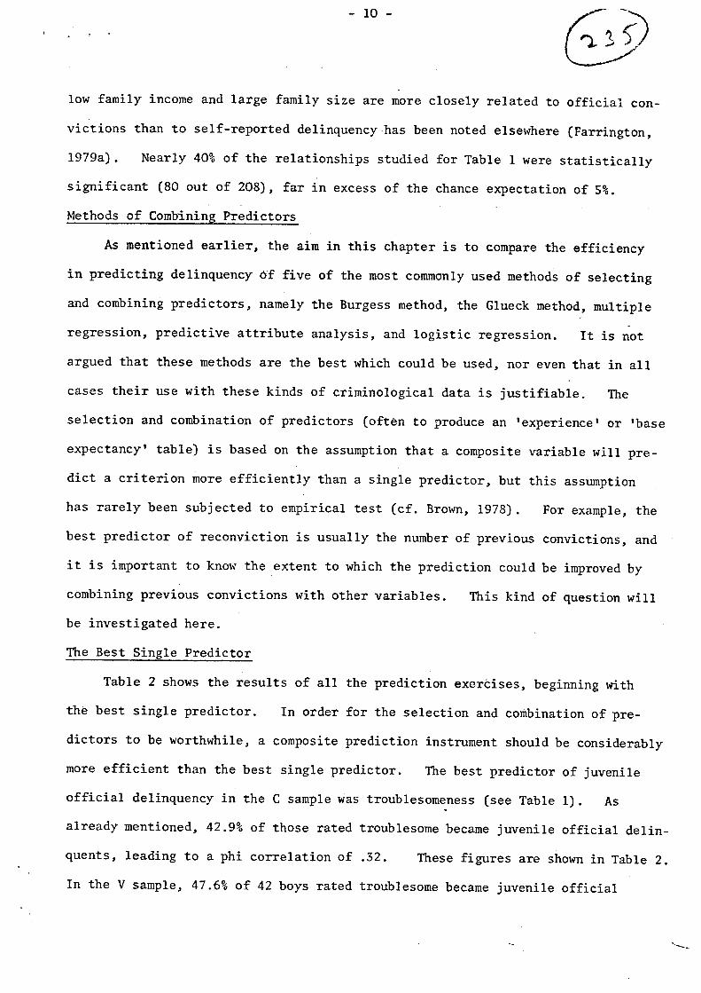
low family income and large family size are more closely related to official con

victions than to self-reported delinquency has been noted elsewhere (Farrington,

1979a). Nearly of the relationships studied for Table were statistically

significant (80 out of 208), far in excess of the chance expectation of

Methods of Combining Predictors

mentioned earlier, the aim in this chapter is to compare the efficiency

in predicting delinquency Of five of the most commonly used methods of selecting

and combining predictors, namely the Burgess method, the Glueck method, multiple

regression, predictive attribute analysis, and logistic regression. It is not

argued that these methods are the best which could be used, nor even that in all

cases their use with these kinds of criminological data is justifiable.

selection and combination of predictors (often to produce an ‘experience’ or ‘base

expectancy’ table) is based on the assumption that a composite variable will pre

dict a criterion more efficiently than a single predictor, but this assumption

has rarely been subjected to empirical test (cf. Brown, 1978). For example, the

best predictor of reconviction is usually the number of previous convictions, and

it is important to the extent to which the prediction could be improved by

combining previous convictions with other variables. This kind of question will

be investigated here.

Best Single Predictor

Table shows the results of all the prediction exerëises, beginning with

the best single predictor. In order for the selection and combination of pre

dictors to be worthwhile, composite prediction instrument should be considerably

more efficient than the best single predictor. best predictor of juvenile

official delinquency in the sample troublesomeness (see Table 1).

already mentioned, 42.9% of those rated troublesome became juvenile official delin

quents, leading to a phi correlation of .32. These figures are in Table 2.

In the sample, of boys rated troublesome became juvenile official

-11-

(,)

15.4% 162 (x2 = p <

= The best predictor official

V was

2

self-reported

in C was parents. 55

self-reported 14.0%

(x2 = < was sig

nificantly predictive V 49 15.5%

x2 = significant, = As

best predictor official C was official

39

11.5% x2 = < =

official significant V

predictor official this was self-

self-

theC onlyjust) was self-reported

41 11.6% 2 = p < =

it was that C was

predictor V The self-reported

V was official

The selecting is that

this, is 1 0

a predictors, on falls

rate. this

ortant

do intercorrelated.

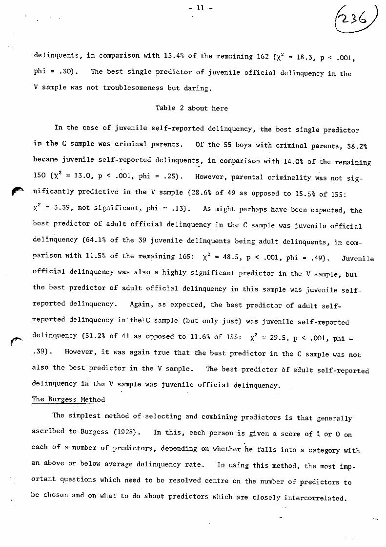
delinquents, in comparison with of the remaining 18.3, .001,

phi .30). single of juvenile delinquency in the

sample not troublesomeness but daring.

Table about here

delinquency,In the case of juvenile the best single predictor

the sample criminal Of the boys with criminal parents, 38.2%

became juvenile delinquents, in comparison with of the remaining

150 13.0, .001, phi .25). However, parental criminalityp not

as opposed toin the sample (28.6% of of 155:

3.39, not .13).phi might perhaps have been expected, the

of adult delinquency in the sample juvenile

delinquency (64.1% of the juvenile delinquents being adult delinquents, in com

parison with of the remaining 165: 48.5, p .001, phi .49). Juvenile

delinquency was also a highly predictor in the sample, but

of adultthe best sampledelinquency in juvenile

reported delinquency. Again, as expected, the best predictor of adult

reported delinquency in sample (but juvenile

delinquency (51.2% of of 155: X 29.5,opposed toas .001, phi

.39). However, again true the best predictor in the sample not

also the best in the sample. best predictor of adult

sampledelinquency in the delinquency.juvenile

The Burgess Method

simplest method of and combining predictors generally

ascribed to Burgess (1928). In personeach or ongiven a score of

each of number of depending whether he into a category with

an above or below average delinquency In using method, the most imp • questions which need to be resolved centre on the number of predictors to

be chosen and on what to about predictors which are closely

was

The

was

was on

1 0

was

known on on was

a 3 on 5

on 3 x

The 7 C

=

low

was a a

Two maximum

6 8

As

49 C

2 46.9% 10.3%

= < =

2 C was

Of 51 V

2 45.1% 14.4%

p < = 2 shows was

Burgess’ score based on virtually all the predictors he had available, but

in Ohlin’s (1951) use of this method he included only predictors which were

associated with the criterion and not closely intercorrelated. method

used here something of a compromise between Burgess and Ohlin. Each pre

based the half-dozen or so factors which were the mostdiction score

closely related to each criterion, disregarding intercorrelations between them.

or on each variable, depending whether the category inEach boy was scored

which he fell associated with an above or below average delinquency rate.

one or moreIf a boy was not the othersvariables, his score

boy scoredincreased pro rata. For example, if points variables and

(6/5)the other, his finalnot knownwas score would be 3.60.or

best predictors of juvenile official delinquency in the sample

(all significant at p .001) were troublesomeness, conduct disorder, acting out,

criminal parents, social handicap, IQ, and poor parental behavior (in that

givenorder). Each prediction score.weight of 1.0 in arriving at

boys in the construction sample had the score of 7, and both were

as werejuvenile official delinquents, of the boys with the next highest

score of 6. with all other variables, the prediction scores were dichotomized

into the ‘worst’ quarter (the group identified as potential delinquents) and the

boys in theremaining three-quarters. Of the sample with prediction scores

of more than points, of thebecame delinquents, in comparison with

remainder (x2 30.0, .001, phi .38).p

Table shows that, in the sample, the Burgess method a slight improve

ment on the best single predictor of troublesomeness, since the percentage of the

identified group becoming delinquents increased from 42.9 to 46.9, and the phi

the boys in the sample scoringcorrelation increased from .32 to .38.

more than points, became delinquents, in comparison with of the

remainder (x2 19.2, .001, phi .31). Table that this very

13

V

Of 7 C

IQ V Two

V

among 7 C

was C

2 shows

was

V was

C was

V Of 6

on

C low

V The was

known a

known

When

On

10 16 th

- -

little improvement over the predictive power of troublesomeness alone in the

sample. the best predictors in the sample, poor parental behavior and

low were not significantly predictive in the sample. of the three

best predictors in the sample, daring and psychomotor clumsiness, were not

the best predictors in the sample, and in fact psychomotor clumsiness

not significantly predictive in the sample.

These analyses were repeated with juvenile self-reported delinquency, adult

official delinquency, and adult self-reported delinquency. Table that

the Burgess method a considerable improvement over the best single predictor

in predicting juvenile self-reported delinquency in the sample. This

because the best single predictor in the sample (criminal parents) not

significantly related in the sample. the best predictors chosen to make

up the prediction score the basis of their relationships with juvenile self-

reported delinquency in the sample (criminal parents, vocabulary, daring,

low IQ, troublesomeness, and social handicap), three were still significantly

predictive in the sample (see Table 1). Burgess method little better

than the best single predictor in predicting adult official delinquency, and

somewhat worse in-predicting adult self-reported delinquency.

These results suggest that, where there is to be good single pre

dictor (as juvenile official delinquency is to be a good predictor of adult

official delinquency), little is gained by the Burgess method. the existence

of a good single predictor is less obvious, the Burgess method is likely to be

better than the best single predictor. the other hand, it must be pointed

out that, apart from juvenile official and self-reported delinquency, no factors

measured between ages and were included in prediction of adult official

and self—reported delinquency. It is possible that later factors combined with

the best single predictor by the Burgess method would have produced an improved

prediction.

-14­

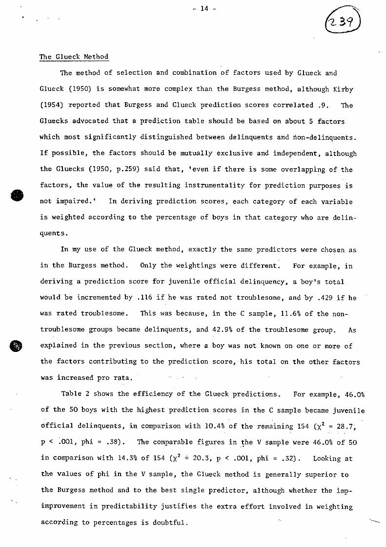
The Glueck Method

The method of selection and combination of factors used by Glueck and

Glueck (1950) is somewhat more complex than the Burgess method, although Kirby

(1954) reported that Burgess and Glueck prediction scores correlated .9. The

Gluecks advocated that a prediction table should be based on about S factors

which most significantly distinguished between delinquents and flon-delinquents.

If possible, the factors should be mutually exclusive and independent, although

the Gluecks (1950, p.259) said that, ‘even if there is some overlapping of the

factors, the value of the resulting instrumentality for prediction purposes is

not impaired.’ In deriving prediction scores, each category of each variable

is weighted according to the percentage of boys in that category who are delin

quent s.

In my use of the Glueck method, exactly the same predictors were chosen as

in the Burgess method. Only the weightings were different. For example, in

deriving a prediction score for juvenile official delinquency, a boy’s total

would be incremented by .116 if he was rated not troublesome, and by .429 if he

was rated troublesome. This was because, in the C sample, 11.6% of the non-

troublesome groups became delinquents, and 42.9% of the troublesome group. As

explained in the previous section, where a boy was not known on one or more of

the factors contributing to the prediction score, his total on the other factors

was increased pro rata.

Table 2 shows the efficiency of the Glueck predictions. For example, 46.0%

of the 50 boys with the highest prediction scores in the C sample became juvenile

official delinquents, in comparison with 10.4% of the remaining 154 (x2 = 28.7,

p < .001, phi = .38). The comparable figures in the V sample were 46.0% of SO

in comparison with 14.3% of 154 (x2 20.3, p < .001, phi = .32). Looking at

the values of phi in the V sample, the Glueck method is generally superior to

the Burgess method and to the best single predictor, although whether the imp

improvement in predictability justifies the extra effort involved in weighting

according to percentages is doubtful.

- -is

Multiple Linear Regression

The Burgess and Glueck methods have been criticized for being subjective

and arbitrary, and for not taking sufficient account of the intercorrelations

between predictors. With the increasing availability of statistical packages

of computer programs such as SPSS, the most common technique now used for selec

ting and combining predictors is probably multiple linear regression, popularized

by Mannheim and Wilkins (1955). With a dichotomous dependent variable, this

is mathematically identical to discriminant analysis (see e.g. Feldhusen,

Aversano and Thurston, 1976). As stated in the introduction, the problem with

multiple regression is that its statistical assumptions are often violated by

criminological data.

The forward stepwise multiple regression technique available in SPSS was

used to obtain weights here. In this, predictor variables are added one at a

time, at each stage adjusting the weights of all the variables in the equation

to produce the greatest possible increase in the multiple correlation between

the actual and predicted values of the criterion. The multiple correlation

approaches its maximum possible value when only a small number of predictors are

included in the equation, and the addition of more predictors does not greatly

increase it. As an example, in predicting juvenile official delinquency in the

C sample, the multiple correlation was .58 with all predictors in the equation.

However, a multiple correlation of .51 was achieved with only 5 predictors, and

one of .55 with 8 predictors. The analysis was carried out under two conditions:

(1) allowing all variables to enter the equation, and (2) adopting an arbitrary

stopping point, such that a predictor was only included in the equation if its

addition produced an increase in the multiple corrqlation of at least .01.

(This corresponded to an increase significant at the .10 level.) The figures

shown in Table 2 are for the multiple regression with a stopping point. For

juvenile delinquency in the C sample, only 8 predictors were included.

16

was

8

7.8% 154 =

< = The was

=

was

- -

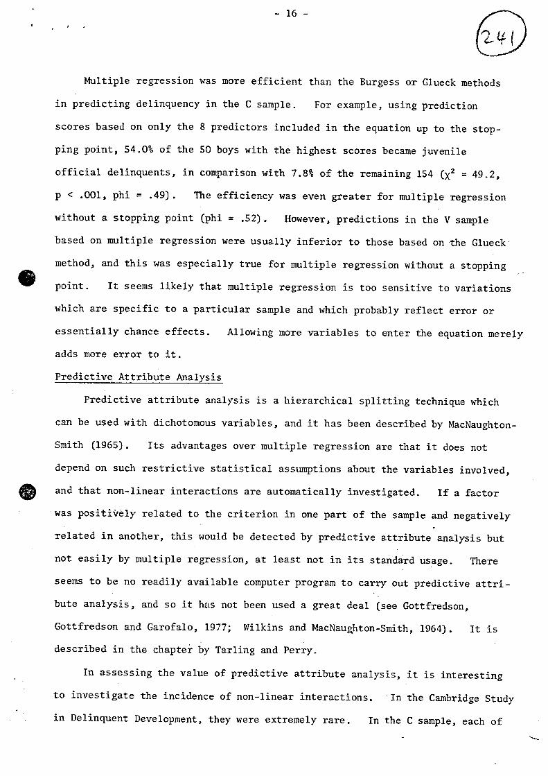
Multiple regression more efficient than the Burgess or Glueck methods

in predicting delinquency in the C sample. For example, using prediction

scores based on only the predictors included in the equation up to the stop

ping point, 54.0% of the 50 boys with the highest scores became juvenile

official delinquents, in comparison with of the remaining (x2 49.2,

p .001, phi .49). efficiency even greater for multiple regression

without a stopping point (phi .52). However, predictions in the V sample

based on multiple regression were usually inferior to those based on the Glueck

method, and this especially true for multiple regression without a stopping

point. It seems likely that multiple regression is too sensitive to variations

which are specific to a particular sample and which probably reflect error or

essentially chance effects. Allowing more variables to enter the equation merely

adds more error to it.

Predictive Attribute Analysis

Predictive attribute analysis is a hierarchical splitting technique which

can be used with dichotomous variables, and it has been described by MacNaughton

Smith (1965). Its advantages over multiple regression are that it does not

depend on such restrictive statistical assumptions about the variables involved,

and that non-linear interactions are automatically investigated. If a factor

was positively related to the criterion in one part of the sample and negatively

related in another, this would be detected by predictive attribute analysis but

not easily by multiple regression, at least not in its standard usage. There

seems to be no readily available computer program to carry out predictive attri

bute analysis, and so it has not been used a great deal (see Gottfredson,

Gottfredson and Garofalo, 1977; Wilkins and MacNaughton—Smith, 1964). It is

described in the chapter by Tarling and Perry.

In assessing the value of predictive attribute analysis, it is interesting

to investigate the incidence of non-linear interactions. In the Cambridge Study

in Delinquent Development, they were extremely rare. In the C sample, each of

-

the four criteria was related to each of the 25 predictors, separately at both

values of each of the other predictors. In only 39 out of 2,400 cases was

there a phi correlation greater than + .10 at one value of a third variable and

-less than .10 at the other. In only 4 cases were the two phi correlations

greater than + .15 and less than - .15. These results agree with those of

Beverly (1964) in showing the rarity of non-linear interaction effects.

The clearest example of an interaction was the relationship between juvenile

self—reported delinquency and secondary school allocation, controlling for vocab

ulary. When vocabulary was low, the boys with low secondary school allocation

were less likely to become juvenile self-reported delinquents (25.0% of 36 as

opposed to 52.0% of 25: X2 = 3.57, p < .10, phi = - .24). In contrast, when

vocabulary was high, the boys with low secondary school allocation were more

likely to become juvenile self-reported delinquents (40.0% of 20 as opposed to

10.1% of 119; x2 = 10.1, significance test not valid, phi = .27). If these

results are not to be attributed to chance, •they may reflect (a) an association

between underachievement (highvocabulary and low school allocation) and delin

quency, and (b) the inability of those with the lowest verbal skills (low vocab

ulary and low school allocation) to report accurately.

As usual, an attempt was made to identify about 50 boys as potential delin

quents, choosing the categories which included the highest percentages who were

delinquents. For example, for juvenile official delinquency in the C sample,

these were (1) 8 troublesome boys with delinquent siblings, (2) 22 troublesome

boys with no delinquent siblings but who were said to be acting out, and (3) 33

boys who were not troublesome but who had criminal parents. This produced a

total of 63 identified boys, of whom 27 were delinqiients (42.9%).

Table 2 shows that the efficiency of predictive attribute analysis was

rather similar to that of multiple regression. Predictive attribute analysis

was usually superior to the Glueck method in the C sample and inferior in the

- -18

V sample. The results obtained with adult official delinquency are artefactual

in the sense that the identified group were all juvenile official delinquents.

There was a very large shrinkage between the C and V samples for juvenile self-

reported delinquency, and this agrees with Simon’s (1971) finding that this

technique can have very large or very small shrinkages in comparison with others.

Logistic Regression

As pointed out in the introduction, logistic regression has rarely been

used in criminology, although it is more suitable than multiple regression, for

example. One practical problem in using it arises from the available computer

package (GLIM) used here, which is far less developed than SPSS.

While using GLIM, it is necessary to investigate the contribution of each predic

tor to the equation rather laboriously, whereas the analogous testing procedure

in stepwise multiple regression is done automatically by SPSS. Fortunately,

with dichotomous variables, multiple and logistic regression tend to select the

same predictors for the equation. Therefore, in order to reduce the time taken

over the logistic regression analyses, they were only carried out with variables

identified (as significant at p = .10) in the multiple regression analyses.

Table 2 shows that, on the basis of the average phi correlation in validation

samples, the logistic regression was the least efficient technique, despite its

theoretical attractions. This was primarily because of the large shrinkage

seen in the analysis of juvenile official delinquency. It seemed that logistic

regression became less efficient in the validation sample as the number of pre

dictors included, in the equation increased, and the same phenomenon was observed

with multiple regression. These techniques may capitalize too heavily on chance

when more than 4 or 5 predictors are included in the equation. However, the

difference between the best technique (Glueck, average phi in V samples .33) and

the worst (logistic regression, .27) was not very great.

was

summary some

3

The

9 20

14 31 10 51 12

102

3

The 3

whom 50%

The was

To 50%

What

Any on

Our on

The

-19­

0 Further CompariSons

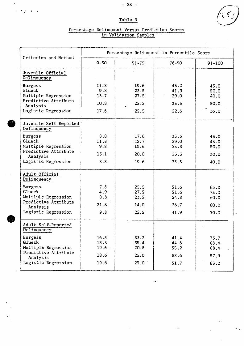
It recommended in the introduction that researchers should not just

present measures of predictive efficiency but should give indication

of the distribution of the criterion over different prediction scores. Table

shows the percentage delinquent in various percentile ranges of prediction scores.

percentile ranges reflect the skewed (J-shapecl) distributions of most predic

tion scores, with a large number bunched at the bottom end (boys not identified potential

as/delinquents on any predictor making up the instrument). For example, in using

the Burgess technique in predicting juvenile official delinquency in the validation

sample, of the boys (45.0%) with the highest scores were delinquents, in

of the next (45.2%), of the next (19.6%), andcomparison with of

the lowest (11.8%). (Where scores were tied, boys were selected in order

of identification number.)

Table about here --

interest in Table is to see the extent to which extremely high predic

tion scores identify a vulnerable group. Even with an extreme category, it seems

more than become juvenile delinto be impossible to identify a group of

predictions of adult delinquency were better, but this probablyquents.

because of the availability of measures of juvenile delinquency as predictors.

Implications for Delinquency Prevention

a statistically significant degree, although with perhaps a false

positive rate, juvenile delinquency can be predicted. ëan be done to prevent

it? attempt to prevent delinquency should be based• explanatory rather

than predictive research. study involved both, and placed most emphasis

early environment and upbringing. educationally retarded children from poor,

socially handicapped, criminal families were especially at risk of committing

-20­

delinquent acts. This suggests that, even at the cost of taking a little away

from the more fortunate members of society, scarce welfare resources should be

concentrated on this vulnerable group. It can be argued that current attempts

to prevent and treat delinquency occur much too late in a person’s life. If

delinquency is part of a larger syndrome beginning in childhood and continuing

into adulthood, as our research suggests, special help and support in the first

few years of life is most likely to be successful.

What options are there for the criminal justice system? Our research sug

gests that convictions do not have their intended (individual deterrent or refor

mative) effects. Boys who were first convicted between ages 14 and 18 had sig

nificantly increased delinquent behavior (as measured by self-report) by the later

age, in comparison with unconvicted boys matched on delinquent behavior at age 14.

A similar result was obtained for first convictions between 18 and 21 (see

Farrington, 1977; Farrington, Osborn, and West, 1978).

As pointed out in the introduction, there has been a great deal of recent

interest in incapacitation as a penal policy. The Cambridge Study data are useful

in investigating incapacitation, because of the availability of self-reports of

offending and official convictions of a fairly representative sample (as opposed

to a sample of detected offenders, on which most of the existing incapacitation

research is based).

During the interview at age 18-19, the boys were asked how many of certain

specified crimes they had committed in the previous 3 years. For example, the

389 boys interviewed reported a total of342 burglaries. During this 3 year

period, 28 of the boys (7.2%) had been convicted of a total of 35 offenses of

burglary, suggesting that the probability of a burglary leading to a conviction

was 10.2%. These 28 convicted boys reported committing 136 burglaries, or 39.8%

of the total admitted by the whole sample. They also reported 223 acts of dam­

— 21

—

aging property of the total of these admitted), 111 of stealing

vehicles of the total), 88 of taking driving away vehicles (20.8%),

of shoplifting (16.0%).

It might therefore predicted that, if there been a sentence

of 3 years incarceration for every convicted burglar 15-18, the total

of crimes in these categories decreased substantially. are

methodological problems with this (see e.g. Blumstein, Nagin,

1978). There is also substantial practical problem. Of the 28 convicted

of burglary, only 7 actually were given institutional sentences for it. Of the

remainder, 9 received probation, 6 received fine, 6 given discharge.

the 7 institutionalized youths, 4 sent to a detention center,

have involved 2 incarceration each. The other 3 going to borstal

to approved school) probably incarcerated for a total of 36

(see Farrington, 1983). The total incarceration actually experienced

these 28 burglars, therefore, 44 months. To incarcerate all 28 for

3 years each mean increasing the average daily population incarcerated a

factor of about is clearly impossible.

Slightly realistically, imagine that the total of incarceration

( for burglary could doubled 44 to 88 months. convicted of burglary

committed average of about 1.6 burglaries per year. Therefore, doubling the

incarceration might possibly have prevented about 6 of the total 342 burglaries

reported - less than 2%. The implications of this analysis are that the probability

of convi-etion for burglary is too the of burglaries

unconvicted is too high for penal policy of incapacitation to effective

in reducing the burglary rate significantly.

Chronic Offenders

Incapacitation is likely to its greatest possible effect on the

rate if it is applied selectively to the persistent offenders, Greenwood

argued. The research of Figlio Sellin that

(35.7% from

(24.3% and

and 194

be had mandatory

aged numbers

would have There

argument Cohen, and

a boys

a and were a

Of were which would

months (two

anand one monthswere

Langan and

by was about.

would by

22, which

more amount

be from Each boy

an

low and number committed by

boys bea

The

have crime

most as

(1982) Wolfgang, and (1972) showed

22

The

more

The 23

17.4% a

10

468

(32.2%

away 30.4%

20.8%

10?

The was

was on

low

— —

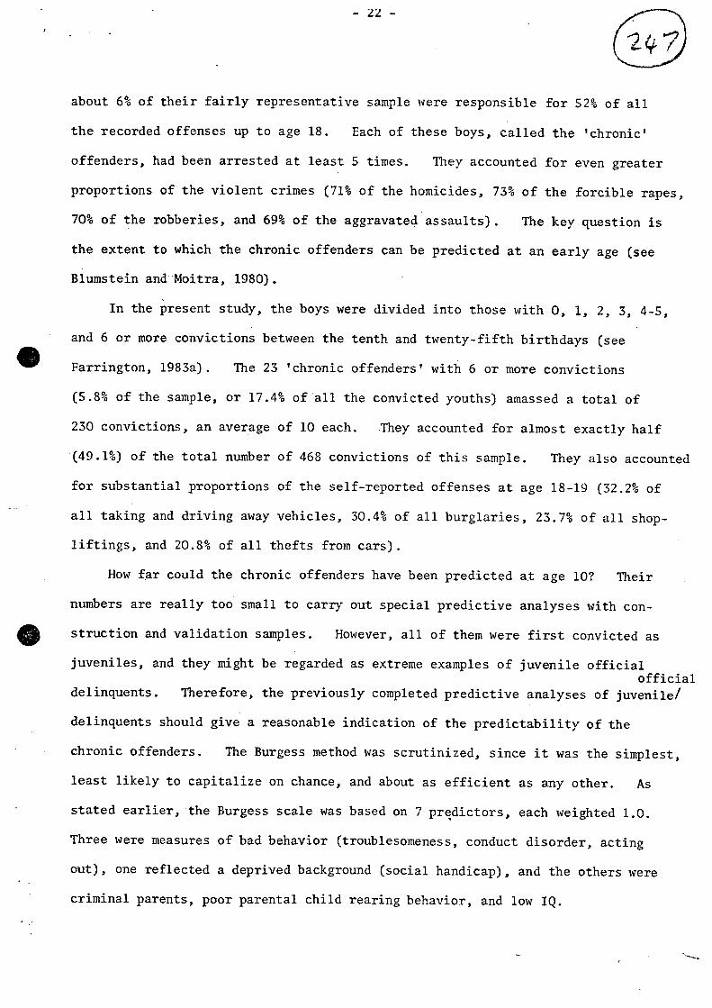
about 6% of their fairly representative sample were responsible for 52% of all

the recorded offenses up to age 18. Each of these boys, called the ‘chronic’

offenders, had been arrested at least 5 times. They accounted for even greater

proportions of the violent crimes (71% of the homicides, 73% of the forcible rapes,

70% of the robberies, and 69% of the aggravated assaults). key question is

the extent to which the chronic offenders can be predicted at an early age (see

Blumstein and Moitra, 1980).

In the present study, the boys were divided into those with 0, 1, 2, 3, 4-5,

and 6 or convictions between the tenth and twenty-fifth birthdays (see

Farrington, 1983a). ‘chronic offenders’ with 6 or more convictions

or(5.8% of the sample, of all the convicted youths) amassed total of

230 convictions, an average of each. They accounted for almost exactly half

(49.1%) of the total number of convictions of this sample. They also accounted

for substantial proportions of the self-reported offenses at age 18-19 of

vehicles,all taking and driving of all burglaries, 23.7% of all shop

liftings, and of all thefts from cars).

How far could the chronic offenders have been predicted at age Their

numbers are really too small to carry out special predictive analyses with con

struction and validation samples. However, all of them were first convicted as

juveniles, and they might be regarded as extreme examples of juvenile official official

delinquents. Therefore, the previously completed predictive analyses of juvenile!

delinquents should give a reasonable indication of the predictability of the

chronic offenders. Burgess method scrutinized, since it was the simplest,

least likely to capitalize on chance, and about as efficient as any other. As

stated earlier, the Burgess scale based 7 predictors, each weighted 1.0.

Three were measures of bad behavior (troublesomeness, conduct disorder, acting

out), one reflected a deprived background (social handicap), and the others were

criminal parents, poor parental child rearing behavior, and IQ.

Taking the construction and validation samples together, 55 boys scored 4

or more out of 7 points on this scale. These included the majority of the

chronic offenders (15 of the 23), 22 other convicted boys (up to the twenty-

fifth birthday), and 18 unconvicted ones. The predictive efficiency was

similar in the construction and validation samples. In the construction sample,

30 boys scored 4 or more, comprising 8 chronic offenders, 11 other convicted boys,

and 11 unconvicted ones. In the validation sample, 25 boys scored 4 or more,

including 7 chronic offenders, 11 otherconvicted youths, and 7 unconvicted ones.

These results suggest that, to a considerable extent, the chronic offenders can

be predicted at age 10.

Conclusions

Returning to the major aims of this chapter, it was difficult to identify a

group with much more than a 50% chance of juvenile delinquency, and conversely

this meant that it was difficult to identify more than 50% of the juvenile delin

quents. It was easier to predict official convictions than self—reported delin

quency, and easier to predict adult offending than juvenile delinquency. The

(

more sophisticated multiple regression, predictive attribute analysis, and

logistic regression techniques were if anything worse than the simpler Burgess

and Glueck methods, although in most instances the Burgess and Glueck methods

were not markedly more efficient than the best single predictor.

There are several possible reasons for the relative inefficiency of delin

quency prediction. One is that relevant predictor variables were not measured.

However, as already mentioned, attempts were made in this project to measure all

variables which were alleged (in 1961) to be causes of delinquency, and information

was obtained from the boys themselves, from their parents, from their teachers,

from their peers, and from official records. A second possible reason is that

the measures of the predictor and criterion variables contained too much error

-24- ,—Th

insensitive. A third

is that on after 10

essentially

How efficiency The

different prediction that it

sophisticated

least

It may that efficiency

valid, reliable, sensitive tech

predictive greater,

sophisticated better, larger is

The results

Ward

this

It realistic

persistent who signifi

all If identified

their first

, A it

institutional significant

effect rate. It it effective,

their

earliest

and, because of the dichotomizing, were too possible reason

delinquency depends events which occur age or which are

unpredictable or due to chance.

of delinquency prediction be improved?could the com

methodsparisons of suggest will not be improved by

devising and using more mathematical methods of selecting and com

bining variables into a prediction instrument, at with our present methods

of measurement. be advances in predictive will only

follow the development of more measurementand

niques. Whether efficiency would be and whether the more

inmethods would perform samples uncertain.

of Babst, Gottfredson and Ballard (1968), with a construction sample

(1968), with a construction sampleof over 3,000, and of of 1,600, are not

in favor of proposition.

morebeseems to and feasible to predict not delinquency in

general but the ‘chronic’ offendersmost or account for a

crime.cant proportion of these people could be at the time

of convictions, they could be subjected to special preventive

measures. policy of incapacitation could not be pursued, because would

require an enormous increase in the population to have a

on the crime and might be morewould be cheaper,

to provide more welfare help and support for these boys and families at the

possible stage.

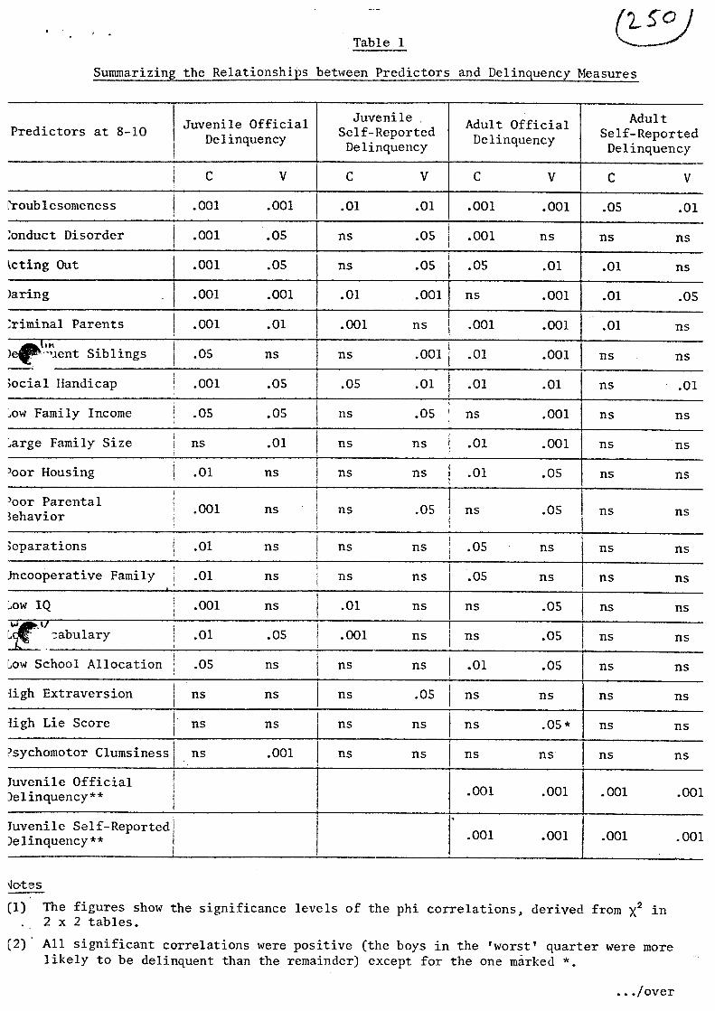
Table 1

Summarizing the Relationships between Predictors and Delinquency Measures

Juvenile Adult Predictors at 8-10

Juvenile Official Self-Reported

Adult Official Delinquency Delinquency Self-Reported

Delinquency Delinquency

C V C V C V C V

roublesomeness .001 .001 .01 .01 .001 .001 .05 .01

onduct Disorder .001 .05 ns .05 .001 ns ns ns

kcting Out .001 .05 ns .05 .05 .01 .01 ns

)aring .001 .001 .01 .001 ns .001 .01 .05

riminal Parents .001 .01 .001 ns .001 .001 .01

I,h)euent Siblings .05 ns ns .001 .01 .001 ns ns

ocial Handicap .001 .05 [ .05 .01 .01 .01 ns .01

.ow Family Income .05 .05 ns .05 ns .001 ns ns

arge Family Size ns .01 ns ns .01 .001 ns ns

‘oor Housing 1 .01 ns ns ns .01 .05 ns ns

‘oor Parental 3ehavior

.001 ns ns .05 ns .05 ns ns

eparations .01 ns ns ns .05 ns ns ns

incooperative Family .01 ns ns ns .05 ns ns ns

ow IQ .001 ns .01 ns ns .05 ns ns 4

Lç Dabulary .01 .05 .001 ns ns .05 ns ns

Low School Allocation .05 ns ns ns .01 .05 ns ns

ugh Extraversion ns ns ns .05 ns ns ns ns

ugh Lie Score ns ns ns ns ns .05* ns ns

‘sychomotor Clumsiness ns .001 ns ns ns ns ns ns

Juvenile Official )elinquency** .001 .001 .001 .001

Juvenile Self-Reported )e linquency ** .001 .001 .001 .001

Ictes

(1) The figures show the significance levels of the phi correlations, derived from 2X in 2 x 2 tables.

(2) All significant correlations were positive (the boys in the ‘worst’ quarter were more likely to be delinquent than the remainder) except for the one marked .

/over

26

(C) (V)

**

The low

- -

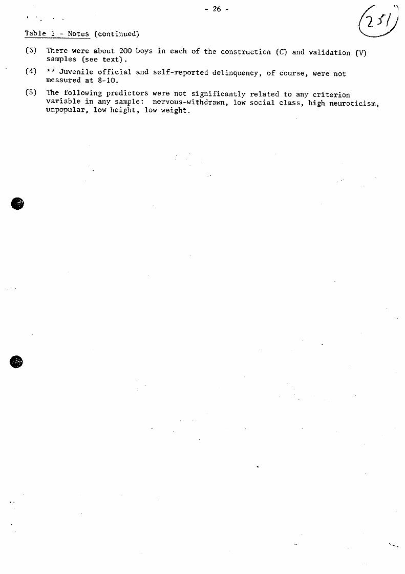
-Table 1 Notes (continued)

(3) There were about 200 boys in each of the construction and validation samples (see text).

(4) Juvenile official and self-reported delinquency, of course, were not measured at 8-10.

(5) following predictors were not significantly related to any criterion variable in any sample: nervous-withdrawn, Unpopular, low height, low weight.

social class, high neuroticism,

Table 2

The Efficiency of Predicting Delinquency

Juvenile Official Juvenile Self-

Adult Official Adult Self- Average Over

Reported Reported DelinquencyDelinquency Delinquency

Delinquency Delinquency MeasuresMethod

19.1 22.1 20.5 18.6 21.6 24.5 19.9 30.1 20.3 23.8 C V C V C V C V C V

Best Single 42.9 47.6 38.2 28.6 64.1 57.8 51.2 61.1 49.1 48.8 Predictor ( .32) ( .30) ( .25) ( .13) ( .49) ( .40) ( .39) ( 3l) ( .36) ( .29)

-Burgess Method 46.9 45.1 42.2 37.5 52.7 58.3 45.5 52.4 46.8 48.3 ( .38) ( .31) ( .27) ( .25) ( .45) ( .42) ( .33) ( .24) ( .36) ( .31)

.Glueck Method 46.0 46.0 46.0 36.0 54.0 60.0 48.1 53.1 48.5 48.8 ( .38) ( .32) ( .34) ( .24) ( .44) ( .46) ( .41) ( 28) ( .39) C .33)

Multiple 54.0 33.3 45.3 35.3 55.6 56.9 49.1 57.7 51.0 45.8 Regression ( .49) C .14) ( .35) ( .23) ( .43) ( .42) ( .43) C .35) ( .43) C .29)

Predictive Attri- 42.9 41.1 48.0 24.5 64.1 57.8 46.6 55.7 50.4 44.8 bute Analysis ( .39) ( .27) ( .37) ( .09) ( .49) ( .40) ( .42) ( .38) C .44) C .29)

Logistic 50.0 27.5 40.4 38.0 62.5 59.1 55.3 56.0 52.1 45.2 Regression ( .43) ( .06) ( .26) C .27) C .48) ( .41) C .48) C .32) ( .41) C .27)

Notes

The figure in each cell shows the percentage of the identified group who became delinquents (official or self-reported). In all cases, the identified group are about 50 of about 200 in each of the con struction (C) and validation (V) samples. The phi correlations are given in brackets. With N = 200, phi = .14 is significant at p = .05, and phi = .23 is significant at p = .001.

I/

- -28

Table 3

Percentage Delinquent Versus Prediction Scoresin Validation Samples

Percentage Delinquent in Percentile Score Criterion and Method

0-50 51-75 76-90 91-100

Juvenile Official I Delinquency

Burgess 11.8 19.6 45.2 45.0 Glueck 9.8 23.5 41.9 50.0 Multiple Regression 13.7 27.5 29.0 40.0 Predictive Attribute Analysis 10.8

— 25.5 35.5 50.0

Logistic Regression 17.6 25.5 22.6 35.0

j Juvenile Self-Reported

t Delinquency

1

Burgess 8.8 17.6 35.5 45.0 Glueck 11.8 15.7 29.0 45.0 Multiple Regression 9.8 19.6 25.8 50.0 Predictive Attribute

Analysis 13.1 20.0 23.3 30.0

Logistic Regression 8.8 19.6 35.5 40.0

Adult Official I Delinquency

Burgess 7.8 25.5 51.6 65.0 Glueck 4.9 27.5 51.6 75.0 Multiple Regression

I Predictive Attribute Analysis

8.8

21.8 1 23.5

14.0

54.8

26.7

60.0

60.0

Logistic Regression 9.8 25.5 41.9 70.0

Adult Self-Reported Delinquency

Burgess 16.5 33.3 41.4 73.7 Glueck 15.5 35.4 44.8 68.4 Multiple Regression 19.6 20.8 55.2 68.4 Predictive Attribute

18.6 25.0 58.6 57.9

Logistic Regression 19.6 25.0 51.7 63.2

D. D. M.,, K. B.

R. home

Academy

A. The

Law

L. D.

A. D. An

E. W.

A. A. A. E. W. The

Law

Law

D. The

D.

C. C. D.

-Z9­

References

Babst, V., Gottfredson, Ballard, (1968). Comparison of

multiple regression and configural analysis techniques for developing

base expectancy tables. Journal of Research in Crime and Delinquency,

5, 72-80.

Beverly, F. (1964). Base expectancies and the initial visit research

schedule. Sacramento: California Youth Authority Research Report 37.

Blumstein, A., Cohen, J., Nagin, 0. (eds., 1978). Deterrence and Incapaci-.

tation. Washington, D.C.: National of Sciences.

Blumstein, E Moitra, S. (1980). identification of ‘career criminals’

from ‘chronic offenders’ in a cohort. and Policy Quarterly, 2,

321-334.

Brown, (1978). The development of a parolee classification system using

discriminant analysis. Journal of Research in Crime and Delinquency,

15, 92-108.

Buckle, Farrington, P. (1983). observational study of shoplifting.

British Journal of Criminology, 23, in press.

Burgess, (1928). Factors determining success or failure on parole. In

Bruce, 3. Harnó, Burgess, 3. Landesco, Workings of

the Indeterminate—Sentence and the Parole System in Illinois.

Springfield, Illinois: Illinois State Board of Parole.

Farrington, 0. P. (1973). Self-reports of deviant behavior: predictive and

stable? Journal of Criminal and Criminology, 64, 99-110.

Farrington, P. (1977). effects of public labelling. British Journal

of Criminology, 17, 112-125.

Farrington, P. (l979a). Environmental stress, delinquent behavior, and

convictions. In I. Sarason Spielberger (eds.) Stress and

Anxiety, vol. 6. Washington, D.C.: Hemisphere.

—30—

D.

N. M. Justice,

D. 10 25 K. Van

A.

press.

D.

D. M. R. J.

New

D. D. J. The

labelling effects. British

D. D. J. The

A. A. B.

J. F., J. R.

Justice

235—253.

B.

, D. M. J. Time in

among risk

Justice,

W.

M. J., J. C.

Hills,

C. correlation.

Farrington, P. (1979b). Longitudinal research on crime and delinquency.

In Morris Tonry (eds.) Crime and vol. 1. Chicago:

University of Chicago Press.

Farrington, to years of age. InP. (l983a). Offending from

MednickDusen S. (eds.) Prospective Studies of Crime and Delinquency.

Boston: Kluwer-Nijhoff, in

Farrington, P. (1983b). Stepping stones to adult criminal careers. In

Block (eds.)’ Development of Antisocial andOlweus, Yarrow

Prosocial Behavior. York: Academic Press, in press.

Farrington, (1978).P., Osborn, S. G., West, persistence of

Journal of Criminology, 18, 277-284.

Farrington, P. West, (1981). Cambridge Study in Delinquent

Mednick andDevelopment. In S. Baert (eds.) Prospective Longi

tudinal Research. Oxford: Oxford University Press.

Feidhusen, Aversano, F. M., Thurston, (1976). Prediction of

youth contacts with law enforcement agencies. Criminal and Behavior,

3,

Glueck, S. Glueck, T. (1950). Unraveling Juvenile Delinquency. Cambridge,

Mass.: Harvard University Press.

Gottfredson, M., Gottfredson, R., Garofalo, (1977). served

paroleeprison and parole outcomes categories. Journal of

Criminal 5, 1-12.

(1982). Selective Incapacitation. Santa Monica, California:Greenwood, P.

Rand Corporation.

Hindelang, Hirschi, T., Weis, (1981). Measuring Delinquency.

California: Sage.Beverly

Kirby, B. (1954). Parole prediction using multiple American

Journal of Sociology, 59, 539-550.

31

La R. A. table

statistics

Law,

D. justice?

Some

Law

Some Statistical

H. L.

L. E. New

H.

G. The differing

New

D. J.

( D. J. Its

D. J. F D. Who Becomes

D. J. D. The Way

L. New classification

i,n

M. R. Sellin,

--

Brie, (1970). Verification of the Glueck prediction by mathe

matical following a computerized procedure of discriminant

function analysis. Journal of Criminal Criminology, and Police

Science, 61, 229-234.

Langan, P. A.. Farrington, P. (1983). Two-track or one-track

evidence from an English longitudinal survey. Journal of Criminal

and Criminology, 74, in press.

MacNaughton-Smith, P. (1965). and Other Numerical Techniques

for Classifying Individuals. London: Her Majesty’s Stationery Office.

Manrtheim, Wilkins, T. (1955). Prediction Methods in Relation to

Borstal Training. London: Her Majesty’s Stationery Office.

Ohlin, (1951). Selection for Parole. York: Russell Sage.

Simon, F. (1971). Prediction Methods in Criminology. London: Her Majesty’s

Stationery Office.

Ward, P. (1968). techniques ofcomparative efficiency of

prediction scaling. Australian and Zealand Journal of Criminology,

1, 109-112.

West, (1969). Present Conduct and Future Delinquency. London: Heinemann.

West, (1982). Delinquency: Roots, Careers, and Prospects. London:

Heinemann.

West, Farrington, P. (1973). Delinquent? London: Heineinann.

West, Farrington, P. (1977). Delinquent of Life. London:

Heinemann.

Wilkins, T. MacNaughton-Smith, P. (1964). prediction and

methods in criminology. Journal of Research Crime and Delinquency, 1,

19-32.

Wolfgang, E., Figlio, M., T. (1972). Delinquency in a Birth

Cohort. Chicago: University of Chicago Press.