Power systems and Queueing theory: Storage andElectric Vehicles

(Joint work with Lisa Flatley, Richard Gibbens, Stan Zachary, SevaShneer)

James Cruise

Maxwell Institute for Mathematical SciencesEdinburgh and Heriot-Watt Universities

December 13, 2017

Plan

Lecture 1: Storage and Arbitrage

Lecture 2: Storage, Buffering and Competition

Lecture 3: Stability and Electric Vehicles

Today:

1 Background

2 The Arbitrage Problem

3 Toy Example - Price taker

4 General Theory - Lagrangian Sufficiency

5 Forecast and Decision Horizon

6 Real Data Example

7 Market Impact

Why do we want electricity storage?

Need to balance supply and demand at all times.

Wind power can fluctuate substantially on a short timescale.

Thermal power plants slow to react.

Can either use expensive alternatives.

Alternatively can use electricity storage.

There are many other uses:

Arbitrage

Frequency regulation

Reactive power support

Voltage support

Black start

Why do we want electricity storage?

Need to balance supply and demand at all times.

Wind power can fluctuate substantially on a short timescale.

Thermal power plants slow to react.

Can either use expensive alternatives.

Alternatively can use electricity storage.

There are many other uses:

Arbitrage

Frequency regulation

Reactive power support

Voltage support

Black start

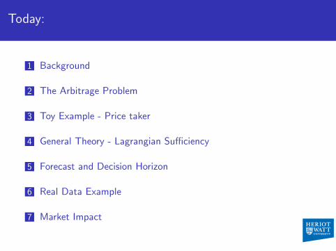
Dinorwig: capacity: 9 GWh rate: 1.8 GW efficiency 0.75–0.80

Storage comes in many forms.

There are many types of storage with different properties:

Pumped storage

Battery storage

Compressed gas storage

Fuel Cells

Thermal

Fly wheels

As well we can consider dynamic demand as storage:

Control of fridges.

Thermal inertia of buildings.

Washing machines.

Aluminium smelting.

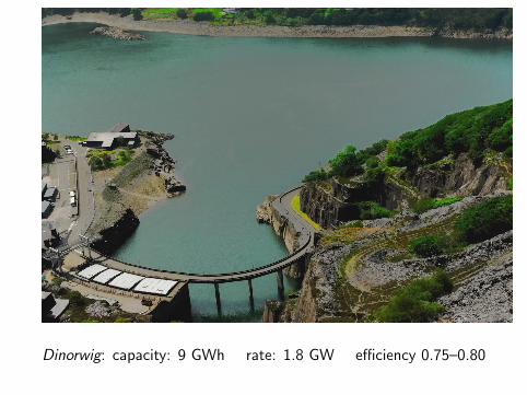
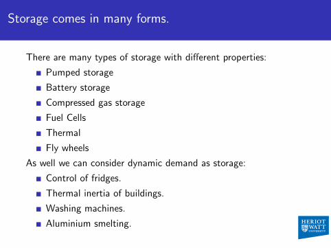
Storage comes in many forms.

There are many types of storage with different properties:

Pumped storage

Battery storage

Compressed gas storage

Fuel Cells

Thermal

Fly wheels

As well we can consider dynamic demand as storage:

Control of fridges.

Thermal inertia of buildings.

Washing machines.

Aluminium smelting.

The Problem:

Storage facilities are expensive, high capital cost.

To facilitate investment we need to understand the value ofstorage.

Today we will only consider money made from arbitrage by anaggregate store.

Sensible since it is expected most of the profit will have comefrom this source.

Need to also be able to compare to alternatives, for exampledemand side management.

Also need to understand the effect of multiple competingstores.

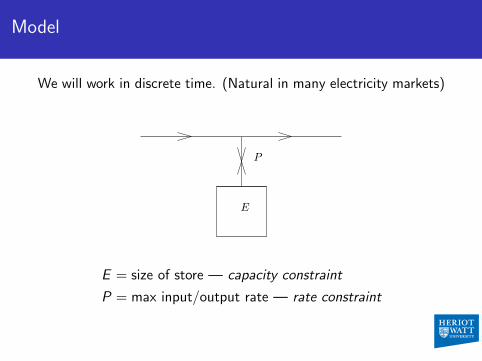
Model

We will work in discrete time. (Natural in many electricity markets)

E

P

E = size of store — capacity constraint

P = max input/output rate — rate constraint

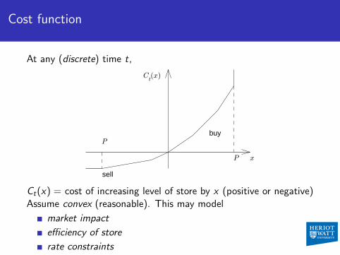
Cost function

At any (discrete) time t,

P

P

sell

buy

x

)x(t

C

Ct(x) = cost of increasing level of store by x (positive or negative)Assume convex (reasonable). This may model

market impact

efficiency of store

rate constraints

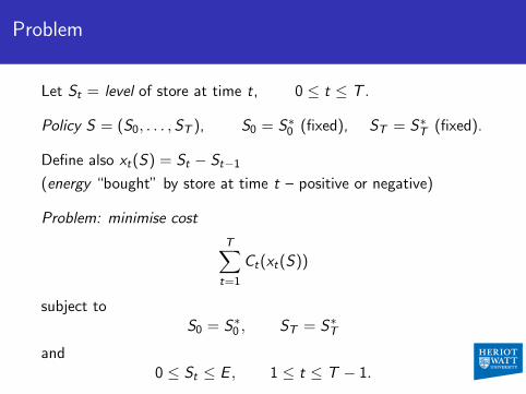
Problem

Let St = level of store at time t, 0 ≤ t ≤ T .

Policy S = (S0, . . . ,ST ), S0 = S∗0 (fixed), ST = S∗

T (fixed).

Define also xt(S) = St − St−1

(energy “bought” by store at time t – positive or negative)

Problem: minimise cost

T∑t=1

Ct(xt(S))

subject toS0 = S∗

0 , ST = S∗T

and0 ≤ St ≤ E , 1 ≤ t ≤ T − 1.

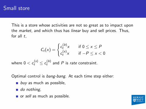
Small store

This is a store whose activities are not so great as to impact uponthe market, and which thus has linear buy and sell prices. Thus,for all t,

Ct(x) =

{c(b)t x if 0 ≤ x ≤ P

c(s)t x if −P ≤ x < 0

where 0 < c(s)t ≤ c

(b)t and P is rate constraint.

Optimal control is bang-bang. At each time step either:

buy as much as possible,

do nothing,

or sell as much as possible.

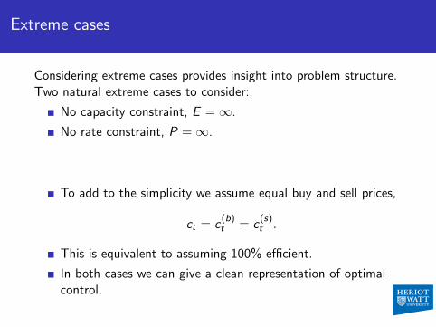
Extreme cases

Considering extreme cases provides insight into problem structure.Two natural extreme cases to consider:

No capacity constraint, E =∞.

No rate constraint, P =∞.

To add to the simplicity we assume equal buy and sell prices,

ct = c(b)t = c

(s)t .

This is equivalent to assuming 100% efficient.

In both cases we can give a clean representation of optimalcontrol.

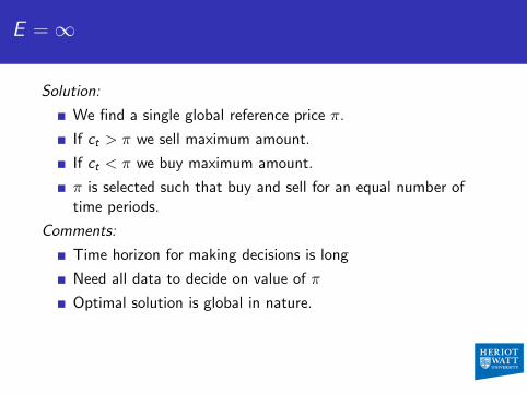
E =∞

Solution:

We find a single global reference price π.

If ct > π we sell maximum amount.

If ct < π we buy maximum amount.

π is selected such that buy and sell for an equal number oftime periods.

Comments:

Time horizon for making decisions is long

Need all data to decide on value of π

Optimal solution is global in nature.

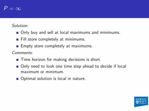
P =∞

Solution:

Only buy and sell at local maximums and minimums.

Fill store completely at minimums.

Empty store completely at maximums.

Comments:

Time horizon for making decisions is short.

Only need to look one time step ahead to decide if localmaximum or minimum.

Optimal solution is local in nature.

Example: Periodic Cost functions

Consider sinusoidal prices.

Interested in what happens as frequency is varied.

Assume P = 1.

Then for a given value of E , there exists a pair µb < µs suchthat we buy if ct < µb and sell if ct > µs .

Further µb is increasing in E and µs is decreasing in E .

Also µb is increasing and µs is decreasing in frequency.

These are bounded by µ∗b and µ∗s , the parameters obtained forE =∞ which does not depend on frequency.

For a given E , as frequency increases profit increases upto theunconstrained case, and there is a frequency beyond whichyou obtain no further benefit.

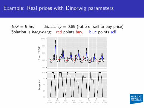
Example: Real prices with Dinorwig parameters

E/P = 5 hrs Efficiency = 0.85 (ratio of sell to buy price).Solution is bang-bang: red points buy, blue points sell

2000

4000

6000

8000

10000P

rices

(£/

MW

h)

0.0

2.5

5.0

7.5

10.0

Sun09−Jan

Mon10−Jan

Tue11−Jan

Wed12−Jan

Thu13−Jan

Fri14−Jan

Sat15−Jan

Sun16−Jan

Sto

rage

leve

l

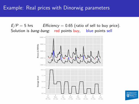
Example: Real prices with Dinorwig parameters

E/P = 5 hrs Efficiency = 0.65 (ratio of sell to buy price).Solution is bang-bang: red points buy, blue points sell

2000

4000

6000

8000

10000P

rices

(£/

MW

h)

0.0

2.5

5.0

7.5

10.0

Sun09−Jan

Mon10−Jan

Tue11−Jan

Wed12−Jan

Thu13−Jan

Fri14−Jan

Sat15−Jan

Sun16−Jan

Sto

rage

leve

l

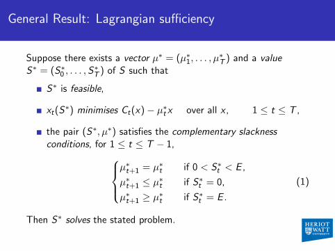
General Result: Lagrangian sufficiency

Suppose there exists a vector µ∗ = (µ∗1, . . . , µ∗T ) and a value

S∗ = (S∗0 , . . . ,S

∗T ) of S such that

S∗ is feasible,

xt(S∗) minimises Ct(x)− µ∗t x over all x , 1 ≤ t ≤ T ,

the pair (S∗, µ∗) satisfies the complementary slacknessconditions, for 1 ≤ t ≤ T − 1,

µ∗t+1 = µ∗t if 0 < S∗t < E ,

µ∗t+1 ≤ µ∗t if S∗t = 0,

µ∗t+1 ≥ µ∗t if S∗t = E .

(1)

Then S∗ solves the stated problem.

Comment

The above result (essentially an application of the LagrangianSufficiency Principle) does not require convexity of thefunctions Ct .

However, convexity the functions Ct is sufficient to guaranteethe existence of a pair (S∗, µ∗) as above.

The latter result is a standard application of StrongLagrangian theory (i.e. the Supporting Hyperplane Theorem).

Algorithm

We need to identify the relevant value of µ∗t at each time t.

It is important to note that the value of µ∗t only changes attimes when the store is full or empty.

Further µ∗t acts as a reference level since the optimal action attime t is given by the x which minimizes:

Ct(x)− µ∗t x .

This is generally equivalent to finding the amount to sell suchthat µ∗t is the marginal price.

We can use this to carry at a search for µ∗.

Further this method is local in time, as we can ignore timesafter filling or emptying the store.

Computational Cost

Careful consideration of how we find µ∗t allows to boundcomputational cost of this process.

Can show we need to carry out at most 2T linear searches ingeneral case.

Work forward from time 0 considering unconstrained problem(Energy).

Find

µut , value need to fill the store at time tµlt , value need to empty the store at time t

Find time when min0,t(µut ) and max0,t(µ

lt) cross.

Definition of Forecast and Decision Horizon

Consider the problem of finding the optimal decision at time 0. Insome problems we can find times:

τ , a Decision Horizon

τ̄ , a Forecast Horizon

Have τ ≤ τ̄Such that:

We can make all optimal decisions up to time τ

With no need for any information after τ̄

So in this example if we can find a pair τ and τ̄ , changing the costfunctions Ct for t > τ̄ will not change the optimal decisions uptotime τ .

Importance of such Horizons

Why do we care?

Often we are making decisions based on forecasts withincreasing uncertainity.

If the forecast horizon is short, do not need much futureknowledge to make decisions.

Allows decomposition of long/infinite horizon problems.

Methodology:

Initially only solve the problem up to the first decision horizon

Extend the solution when this time is reached.

Horizons and Coupling

Forecast horizons often occur because of path coupling.

Examples include:

Trunking

Holding costs

Constrained state space

Existence of Horizons

The constraint on the store level (between 0 and E ) leads to aforecast horizon.

Paths couple as squeezed against boundaries

Similar to ideas from coupling from the past.

Means that the forecast horizon length is on the order thelength of the filling/emptying cycle.

In many examples this will be on the order of a 1 or 2 days inreality.

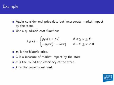
Example

Again consider real price data but incorporate market impactby the store.

Use a quadratic cost function:

Ct(x) =

{ptx(1 + λx) if 0 ≤ x ≤ P

−ptνx(1 + λνx) if −P ≤ x < 0

pt is the historic price.

λ is a measure of market impact by the store.

ν is the round trip efficiency of the store.

P is the power constraint.

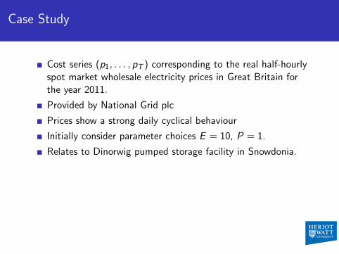
Case Study

Cost series (p1, . . . , pT ) corresponding to the real half-hourlyspot market wholesale electricity prices in Great Britain forthe year 2011.

Provided by National Grid plc

Prices show a strong daily cyclical behaviour

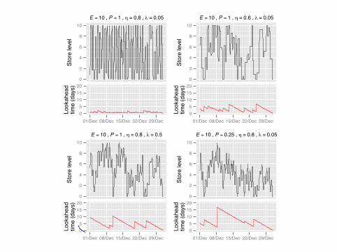
Initially consider parameter choices E = 10, P = 1.

Relates to Dinorwig pumped storage facility in Snowdonia.

0

2

4

6

8

10

Stor

e le

vel

E = 10 , P = 1 , η = 0.8 , λ = 0.05

05

101520

01/Dec 08/Dec 15/Dec 22/Dec 29/Dec

Look

ahea

dtim

e (d

ays)

0

2

4

6

8

10

Stor

e le

vel

E = 10 , P = 1 , η = 0.6 , λ = 0.05

05

101520

01/Dec 08/Dec 15/Dec 22/Dec 29/Dec

Look

ahea

dtim

e (d

ays)

0

2

4

6

8

10

Stor

e le

vel

E = 10 , P = 1 , η = 0.8 , λ = 0.5

05

101520

01/Dec 08/Dec 15/Dec 22/Dec 29/Dec

Look

ahea

dtim

e (d

ays)

0

2

4

6

8

10

Stor

e le

vel

E = 10 , P = 0.25 , η = 0.8 , λ = 0.05

05

101520

01/Dec 08/Dec 15/Dec 22/Dec 29/Dec

Look

ahea

dtim

e (d

ays)

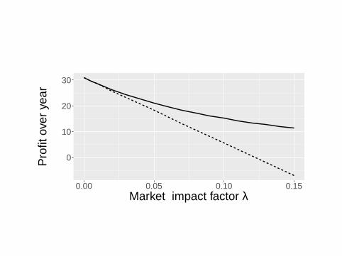
0

10

20

30

0.00 0.05 0.10 0.15Market impact factor λ

Pro

fit o

ver

year

Market impact of storage

A large store may impact costs (be a price-maker), and hence therest of society.

Impact of storage on consumer surplus is in general beneficial,but not necessarily.

Example (T = 2): Buy x at time 1 (increasing price by p1) andsell at time 2 (decreasing price by p2).

Increase in consumer surplus is

p2d2 − p1d1

where d1 and d2 are the respective demands at times 1 and 2.

In general expect d2 > d1 and p2 to be comparable to p1, so effecton consumer surplus is beneficial.

However, the latter need not be the case.

Market impact of storage

A large store may impact costs (be a price-maker), and hence therest of society.

Impact of storage on consumer surplus is in general beneficial,but not necessarily.

Example (T = 2): Buy x at time 1 (increasing price by p1) andsell at time 2 (decreasing price by p2).

Increase in consumer surplus is

p2d2 − p1d1

where d1 and d2 are the respective demands at times 1 and 2.

In general expect d2 > d1 and p2 to be comparable to p1, so effecton consumer surplus is beneficial.

However, the latter need not be the case.

Market impact of storage

A large store may impact costs (be a price-maker), and hence therest of society.

Impact of storage on consumer surplus is in general beneficial,but not necessarily.

Example (T = 2): Buy x at time 1 (increasing price by p1) andsell at time 2 (decreasing price by p2).

Increase in consumer surplus is

p2d2 − p1d1

where d1 and d2 are the respective demands at times 1 and 2.

In general expect d2 > d1 and p2 to be comparable to p1, so effecton consumer surplus is beneficial.

However, the latter need not be the case.