Embed Size (px)
Citation preview
Potential Outcome and Directed Acyclic Graph
Approaches to Causality: Relevance for
Empirical Practice in Economics∗
Guido W. Imbens†
March 2020
Abstract
In this essay I discuss potential outcome and graphical approaches to causality, and their
relevance for empirical work in economics. I review some of the work on directed acyclic
graphs, including the recent “The Book of Why,” ([Pearl and Mackenzie, 2018]). I also
discuss the potential outcome framework developed by Rubin and coauthors (e.g., [Rubin,
2006]), building on work by Neyman ([Neyman, 1923/1990]). I then discuss the relative
merits of these approaches for empirical work in economics, focusing on the questions each
framework answer well, and why much of the the work in economics is closer in spirit to
the potential outcome perspective.
∗I am grateful for help with the graphs by Michael Pollmann and for comments by Alberto Abadie,Jason Abaluck, Alexei Alexandrov, Josh Angrist, Susan Athey, Gary Chamberlain, Stephen Chaudoin,Rebecca Diamond, Dean Eckles, Ernst Fehr, Avi Feller, Paul Goldsmith-Pinkham, Chuck Manski,Paul Milgrom, Evan Munro, Franco Perrachi, Michael Pollmann, Thomas Richardson, Jasjeet Sekhon,Samuel Skoda, Korinayo Thompson, and Heidi Williams. They are not responsible for any of the viewsexpressed here. Financial support from the Office of Naval Research under grant N00014-17-1-2131 isgratefully acknowledged. The first version of this paperwas circulated in May 2019.†Professor of Economics, Graduate School of Business, and Department of Economics, Stanford
University, SIEPR, and NBER, [email protected].
arX
iv:1
907.
0727
1v2
[st
at.M
E]
22
Mar
202
0

1 Introduction
Causal Inference (CI) in observational studies has been an integral part of econometrics since its
start as a separate field in the 1920s and 1930s. The simultaneous equations methods developed
by [Tinbergen, 1930], [Wright, 1928], [Haavelmo, 1943], and their successors in the context of
supply and demand settings were from the beginning, and continue to be, explicitly focused on
causal questions. Subsequently, the work by the Cowles commission, and both the structural
and reduced form approaches since then, have thrived by focusing on identifying and estimating
causal and policy-relevant parameters. Over the last thirty years close connections to related
research on causal inference in other social sciences and statistics, and, more recently, computer
science have been established. In this essay I review some of the approaches to causal inference in
the different disciplines in the context of some recent textbooks, and discuss the relevance of these
perspectives for empirical work in economics. The two main frameworks are (i) the Potential
Outcome (PO) framework, associated with the work by Donald Rubin, building on the work on
randomized controlled trials (RCTs) from the 1920s by Ronald Fisher and Jerzey Neyman, and
(ii) the work on Directed Acyclic Graphs (DAGs), much of it associated with work by Judea
Pearl and his collaborators. These frameworks are complementary, with different strengths that
make them particularly appropriate for different questions. Both have antecedents in the earlier
econometric literature, the PO framework in the demand and supply models in [Tinbergen,
1930] and [Haavelmo, 1943], and the DAG approach in the path analysis in [Wright, 1928].
The body of this essay consists of three parts. In the first part of the essay I discuss the
graphical approach to causality in the context of the recent book “The Book of Why” (TBOW)
by Judea Pearl and Dana Mackenzie [Pearl and Mackenzie, 2018], which is a very accessible
introduction to this approach. I highly recommend both TBOW and the more technical and
comprehensive [Pearl, 2000] for anyone who is interested in causal inference in statistics, and
that should include pretty much anyone doing empirical work in social sciences these days. The
graphical approach has gained much traction in the wider computer science community, see
for example the recent text “Elements of Causal Inference,” ([Peters, Janzing, and Scholkopf,
2017]) and the work on causal discovery ([Glymour, Scheines, and Spirtes, 2014, Hoyer, Janz-
ing, Mooij, Peters, and Scholkopf, 2009, Lopez-Paz, Nishihara, Chintala, Scholkopf, and Bottou,
2017, Ke, Bilaniuk, Goyal, Bauer, Larochelle, Pal, and Bengio, 2019]) and interpretability (citet-
zhao2019causal), and also in parts of epidemiology and social sciences, although it has not had as
1
much impact in economics as it should have Exceptions include the methodological discussions
in White and Chalak [2006, 2009], Chalak and White [2011], Heckman and Pinto [2015], and the
recent discussions on on the benefits graphical causal modeling for economics in Cunningham
[2018], Hunermund and Bareinboim [2019].
In the second part of this essay, in Section 3, I review the potential outcome approach,
associated with the work by Donald Rubin, Paul Rosenbaum, and collaborators, that is more
familiar to economists. Representative of the methodological part of the potential outcome
literature is the collection of papers by Rubin and coauthors, “Matched Sampling for Causal
Effects,” (MACE, [Rubin, 2006]) and “Observation and Experiment,” ([Rosenbaum, 2017]).
Other references to this literature include [Rubin, 1974, Rosenbaum, 2002, 2010], [Holland,
1986] which coined the term “Rubin Causal Model” for this approach, and my own text with
Rubin, “Causal Inference in Statistics, Social, and Biomedical Sciences,” (CISSB, [Imbens and
Rubin, 2015]).1
In the third and main part of this essay, in Section 4, I discuss the comparative strengths and
weaknesses of the PO and DAG approaches. I discuss why the graphical approach to causality
has not caught on very much (yet) in economics. For example, a recent econometrics textbook
focused on causal inference, Mostly Harmless Econometrics (MHE, [Angrist and Pischke, 2008]),
has no DAGs, and is largely in the PO spirit. Why has it not caught on, or at least not yet?
At a high level the DAG approach has two fundamental benefits to offer. First, in what is
essentially an pedagogical component, the formulation of the critical assumptions is intended to
capture the way researchers think of causal relationships. The DAGs, like the path analyses that
came before them ([Wright, 1928, 1934]), can be a powerful way of illustrating key assumptions
in causal models. I elaborate on this aspect of DAGs in the discussions of instrumental variables
and mediation/surrogates. Ultimately some of this is a matter of taste and some researchers
may prefer graphical versions to algebraic versions of the same assumptions and vice versa.
Second, the machinery developed in the DAG literature, in particular the do-calculus discussed
in Section 2.5, aims to allow researchers to answer particular causal queries in a systematic
way. Here the two frameworks are complementary and have different strengths and weaknesses.
The DAG machinery simplifies the answering of certain causal queries compared to the PO
framework. This is particularly true for queries in complex models with a large number of
1As a disclaimer, I have worked with both Rubin and Rosenbaum, and my own work on causal inference islargely within the PO framework, although some of that work preceeds these collaborations.
2
variables. However, there are many causal questions in economics for which this is is not true.
In comparison, there are five features of the PO framework that may be behind its cur-
rent popularity in economics. First, there are some assumptions that are easily captured in
the PO framework relative to the DAG approach, and these assumptions are critical in many
identification strategies in economics. Such assumptions include monotonicity ([Imbens and
Angrist, 1994]) and other shape restrictions such as convexity or concavity ([Matzkin et al.,
1991, Chetverikov, Santos, and Shaikh, 2018, Chen, Chernozhukov, Fernandez-Val, Kostyshak,
and Luo, 2018]). The instrumental variables setting is a prominent example where such shape
restrictions are important, and I will discuss it in detail in Section 4.2. Second, the potential
outcomes in the PO framework connect easily to traditional approaches to economic models such
as supply and demand settings where potential outcome functions are the natural primitives.
Related to this, the insistence of the PO approach on manipulability of the causes, and its at-
tendant distinction between non-causal attributes and causal variables has resonated well with
the focus in empirical work on policy relevance ([Angrist and Pischke, 2008, Manski, 2013b]).
Third, many of the currently popular identification strategies focus on models with relatively
few (sets of) variables, where identification questions have been worked out once and for all.
Fourth, the PO framework lends itself well to accounting for treatment effect heterogeneity in
estimands ([Imbens and Angrist, 1994, Sekhon and Shem-Tov, 2017]) and incorporating such
heterogeneity in estimation and the design of optimal policy functions ([Athey and Wager, 2017,
Athey, Tibshirani, Wager, et al., 2019b, Kitagawa and Tetenov, 2015]). Fifth, the PO approach
has traditionally connected well with questions of study design, estimation of causal effects and
inference for such effects. From the outset Rubin and his coauthors provided much guidance to
researchers and policy makers for practical implementation including inference, with the work
on the propensity score ([Rosenbaum and Rubin, 1983b]) an influential example.
Separate from the theoretical merits of the two approaches, another reason for the lack of
adoption in economics is that the DAG literature has not shown much evidence of the alleged
benefits for empirical practice in settings that resonate with economists. The potential out-
come studies in MACE, and the chapters in [Rosenbaum, 2017], CISSB and MHE have detailed
empirical examples of the various identification strategies proposed. In realistic settings they
demonstrate the merits of the proposed methods and describe in detail the corresponding esti-
mation and inference methods. In contrast in the DAG literature, TBOW, [Pearl, 2000], and
[Peters, Janzing, and Scholkopf, 2017] have no substantive empirical examples, focusing largely
3
on identification questions in what TBOW refers to as “toy” models. Compare the lack of
impact of the DAG literature in economics with the recent embrace of regression discontinuity
designs imported from the psychology literature, or with the current rapid spread of the machine
learning methods from computer science, or the recent quick adoption of synthetic control meth-
ods developed in economics [Abadie and Gardeazabal, 2003, Abadie, Diamond, and Hainmueller,
2010]. All three came with multiple concrete and detailed examples that highlighted their ben-
efits over traditional methods. In the absence of such concrete examples the toy models in the
DAG literature sometimes appear to be a set of solutions in search of problems, rather than a
set of clever solutions for substantive problems previously posed in social sciences, bringing to
mind the discussion of Leamer on the Tobit model ([Leamer, 1997]).
2 The Graphical Approach to Causality and TBOW
In this section I review parts of TBOW and give a brief general introduction to Directed Acyclic
Graphs (DAGs).
2.1 TBOWs View of Causality, and the Questions of Interest
Let me start by clarifying what TBOW, and in general the DAG approach to causality is
interested in. The primary focus of TBOW, as well as [Pearl, 2000], is on identification, as
opposed to estimation and inference. As Figure 1 (TBOW, p. 12) illustrates, researchers arrive
armed with a number of variables and a causal model linking these variables, some observed and
some unobserved. The assumptions underlying this model are coded up in a graphical model, a
Directed Acyclic Graph, or DAG. The researchers then ask causal queries. Early in TBOW the
authors present some examples of such questions (TBOW, p. 2):
1. How effective is a given treatment in preventing a disease?
2. Did the new tax law cause our sales to go up, or was it our advertising campaign?
3. What is the health-care cost attributable to obesity?
4. Can hiring records prove an employer is guilty of a policy of sex discrimination?
5. I’m about to quit my job. Should I?
4
These types of questions are obviously all of great importance. Does the book deliver on this,
or more precisely, does the methodology described in the book allow us to answer them? The
answer essentially is an indirect one: if you tell me how the world works (by giving me the full
causal graph), I can tell you the answers. Whether this is satisfactory really revolves around
how much the researcher is willing to assume about how the world works. Do I feel after reading
the book that I understand better how to answer these questions? That is not really very clear.
The rhetorical device of giving these specific examples at the beginning of the book is very
helpful, but the book does not really provide context for them. Questions of this type have
come up many times before, but there is little discussion of the previous approaches to answer
them. The reader is never given the opportunity to compare previously proposed answers. It
would have been helpful for the reader if in the final chapter TBOW would have returned to
these five questions and described specific answers given the book to these five questions and
then compared them to alternative approaches. Instead some of the questions come back at
various stages, but not systematically, and the impression is created that it was not possible to
answer these questions previously.
One class of questions that is missing from this list, somewhat curiously given the title of
TBOW, is explicitly “why” questions. Why did Lehmann Brothers collapse in 2008? Why did
the price of a stock go up last year? Why did unemployment go down in the Great Depression?
[Gelman and Imbens, 2013] refer to such questions as reverse causal inference question, “why”
an outcome happened, rather than forward causal questions that are concerned with the effect
of a particular manipulation. The causal literature in general has focused much less on such
reverse causal questions.
The focus of TBOW, [Pearl, 2000] and [Peters, Janzing, and Scholkopf, 2017], is on develop-
ing machinery for answering questions of this type given two inputs. First, knowledge of the joint
distribution of all the observed variables in the model, and, second, a causal model describing
the phenonoma under consideration. Little is said about what comes before the identification
question, namely the development of the model, and what comes after the identification ques-
tion, namely estimation and inference given a finite sample. The position appears to be that the
specification of a causal model and the statistical analyses are problems separate from those of
identification, with the integration of those problems with questions of identification less impor-
tant than the benefits of the specialization associated with keeping the identification questions
separate.
5
However, many statistical problems and methods are specific to the causal nature of the
questions, and as a result much of the methodological literature on causality in statistics and
econometrics is about estimation methods. This includes the literature on weak instruments
[Staiger and Stock, 1997, Andrews and Stock, 2006], the literature on unconfoundedness in-
cluding discussions of the role of the propensity score ([Rosenbaum and Rubin, 1983b]) and
problems with overlap ([Crump, Hotz, Imbens, and Mitnik, 2009, D’Amour, Ding, Feller, Lei,
and Sekhon, 2017, Li, Morgan, and Zaslavsky, 2018]), double robustness [Robins and Rotnitzky,
1995, Imbens, 2004, Belloni, Chernozhukov, Fernandez-Val, and Hansen, 2013, Athey, Imbens,
and Wager, 2018b], the literature on regression discontinuity designs [Hahn, Todd, and Van der
Klaauw, 2001, Imbens and Kalyanaraman, 2012], and the recent work on estimating heteroge-
nous treatment effects [Athey and Imbens, 2016, Wager and Athey, 2017] and synthetic control
methods ([Abadie and Gardeazabal, 2003, Abadie, Diamond, and Hainmueller, 2010]. Another
area where the separation between identification of causal effects and the identification of the
joint distribution of realized variables is more difficult is in network settings [Graham, 2015,
Ogburn, VanderWeele, et al., 2014, Athey, Eckles, and Imbens, 2018a]. This integration of sta-
tistical questions and causal identification has arguably been very beneficial in many of these
settings.
The choices and challenges in postulating a causal model, graphical or otherwise, that is, a
model of how the world works, is also not a major subject of the book. TBOW views that as
the task of subject matter experts:
“I am not a cancer specialist, and I would always have to defer to the expert opinion
on whether such a diagram represents and real-world processes accurately.” (TBOW,
p. 228)
and
“I am not personally an expert on climate change‘’ (TBOW, p. 294)
This is of course fine, but the result is that the models in TBOW are all, in a favorite phrase of
Pearl’s, “toy models,” suggesting that we should not take them too seriously. This is common
to other discussions of graphical causal models (e.g., [Koller, Friedman, and Bach, 2009]). It
would have been useful if the authors had teamed up with subject matter experts and discussed
some substantive examples where DAGs, beyond the very simple ones implied by randomized
6
experiments, are aligned with experts’ opinions. Such examples, whether in social sciences or
otherwise, would serve well in the effort to convince economists that these methods are useful
in practice.
The focus on toy models and the corresponding lack of engagement with estimation and
inference questions is in sharp contrast to the econometrics literature where the three steps, (i)
the development of the causal models that preceeds the identification question, (ii) the study of
identification questions, and (iii) estimation and inference methods that follow once the iden-
tification questions have been resolved, typically go hand-in-hand. The models in econometric
papers are often developed with the idea that they are useful on settings beyond the specific
application in the original paper. Partly as a result of the focus on empirical examples the econo-
metrics literature has developed a small number of canonical settings where researchers view
the specific causal models and associated statistical methods as well-established and understood.
These causal models correspond to what is nowadays often referred to as identification strate-
gies (e.g., [Card, 1993, Angrist and Krueger, 2000]). These identification strategies that include
adjustment/unconfoundedness, instrumental variables, difference-in-differences, regression dis-
continuity designs, synthetic control methods (the first four are listed in “Empirical Strategies in
Labor Economics,” [Angrist and Krueger, 2000]) are widely taught in both undergraduate and
graduate economics courses, and they are familiar to most empirical researchers in economics.
The statistical methods associated with these causal models are commonly used in empirical
work and are constantly being refined, and new identification strategies are occasionally added
to the canon. Empirical strategies not currently in this canon, rightly or wrongly, are viewed
with much more suspicion until they reach the critical momentum to be included. This canon
is not static: despite having been developed in the early 1960s in the psychology literature,
regression discontinuity designs were virtually unheard of in economics until the early 2000s
when a number of examples caught researchers’ attention (e.g., [Black, 1999, Van Der Klaauw,
2002, Lee, Moretti, and Butler, 2010, Pettersson-Lidbom, 2008]). Now regression discontinuity
designs are commonly taught in graduate and undergraduate courses. Similarly synthetic con-
trol methods ([Abadie, Diamond, and Hainmueller, 2010]) have become very popular in a very
short period of time, and are a staple of graduate econometrics courses.
7
2.2 The Ladder of Causality
TBOW introduces a classification of causal problems that they call the Ladder of Causality,
with three rungs, in order of complexity labeled association, intervention, and counterfactuals
respectively.
On the first rung, assocation, researchers observe passively, and form predictions based on
these observations. A key concept is that of correlation or association. Methods belonging to this
rung according to the discussion in TBOW are regression, as well as many of the modern machine
learning methods such as regression trees, random forests, and deep neural nets. Of course
regression is used in many disciplines as a causal method, but here TBOW views regression
in something akin to what econometricians would call the best linear predictor framework,
where the regression function is simply a parametric way of fitting the conditional expectation
[Goldberger, 1991]. There is little causal in this rung, and the problems here are well understood
and continue to be studied in a variety of disciplines. They are routinely taught in economics
PhD programs as part of the econometrics or statistics curriculum. Much of this is now being
integrated with predictive machine learning methods ([Athey and Imbens, 2018]).
The second rung is that of intervention. A canonical example, used in Figure 1.2 (TBOW,
p. 28), and also in CISSB (p. 3), is the question what would happen to my headache if I
take an aspirin. In general the questions in this rung are about manipulations. These are the
questions that much of the causal inference work in the PO framework is focused on. Randomized
experiments are one of the key statistical designs here. In observational studies these questions
are much harder, but they are studied in a wide range of areas using a wide range of methods.
Question 1 in the list of questions in TBOW (“How effective is a given treatment in preventing
a disease?”) belongs on this rung. This is where much of the empirical work in economics takes
place. The challenges typically concern the presence of unobserved confounders of some type
or another because economist typically model the behavior of optimizing agents, who often are
more knowledgable than the researcher and who take into account the expected results of their
actions. The identification strategies in [Angrist and Krueger, 2000] fit in here.
The third rung of the ladder of causality deals with counterfactuals. Here the type of ques-
tion considered is “What would have happened had I not taken the aspirin?” [given that I did
take the aspirin, GWI] (TBOW, p. 33). The questions on this third run are more difficult to
answer, and the PO framework is more apprehensive about definite answers to such questions
8
that depend delicately on individual-level heterogeneity. In the PO framework the correlation
between the potential outcomes given the aspirin and without the aspirin, within subpopula-
tions homogenous in observed characteristics, is not point-identified, As a result estimands that
depend on this correlation, which includes most questions on the third rung, are only partially
identified. Although in legal settings this type of question does come up routinely in so-called
“but-for” analyses,2 the economics literature does not focus as much on this type of question as
it does on the second type.
Related to the issue raised in the discussion in Section 2.1 of the list of questions provided
in TBOW, I would have liked to have seen a fourth rung of the ladder, dealing with “why,” or
reverse causality questions ([Gelman and Imbens, 2013]). Such questions are related to both the
second and third rung, but not quite the same.
2.3 Directed Acyclic Graphs
The approach to causality in TBOW and [Pearl, 2000] centers on graphical models, and in
particular Directed Acyclic Graphs (DAGs). These are seen as an attractive way to capture
how people think about causal relationships. The DAGs are characterized by nodes and directed
edges between the nodes. Let us start with four examples, in increasing order of complexity.
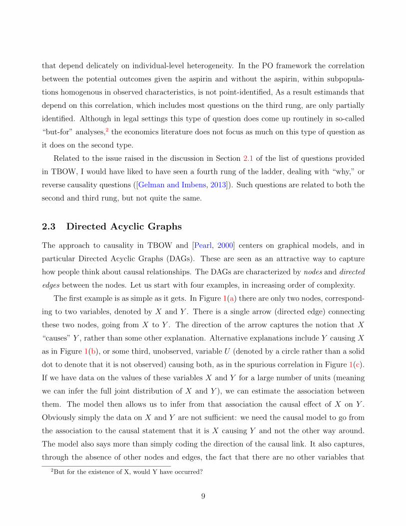
The first example is as simple as it gets. In Figure 1(a) there are only two nodes, correspond-
ing to two variables, denoted by X and Y . There is a single arrow (directed edge) connecting
these two nodes, going from X to Y . The direction of the arrow captures the notion that X
“causes” Y , rather than some other explanation. Alternative explanations include Y causing X
as in Figure 1(b), or some third, unobserved, variable U (denoted by a circle rather than a solid
dot to denote that it is not observed) causing both, as in the spurious correlation in Figure 1(c).
If we have data on the values of these variables X and Y for a large number of units (meaning
we can infer the full joint distribution of X and Y ), we can estimate the association between
them. The model then allows us to infer from that association the causal effect of X on Y .
Obviously simply the data on X and Y are not sufficient: we need the causal model to go from
the association to the causal statement that it is X causing Y and not the other way around.
The model also says more than simply coding the direction of the causal link. It also captures,
through the absence of other nodes and edges, the fact that there are no other variables that
2But for the existence of X, would Y have occurred?
9
X Y
(a) Randomized Experiment
X Y
(b) Reverse Causality
X Y
U
(c) Spurious Correlation
X Y
U2U1
(d) Randomized Experiment (AlternativeDAG)
Figure 1: DAGs for the Two Variable Case
X Y
W
Figure 2: Unconfoundedness
have causal effects on both X and Y as, for example, in Figure 1(c). Note that we could expand
the DAG by including two unobserved variables, U1 and U2, with an arrow (U1 → X) and an
arrow (U2 → Y ), as in Figure 1(d). In the Structural Equation Model (SEM) version of the
DAGs these unobserved variables would be explicit. Because there is no association between U1
and U2, the presence of these two unobserved variables does not affect any conclusions, so we
omit them from the DAG, following convention.
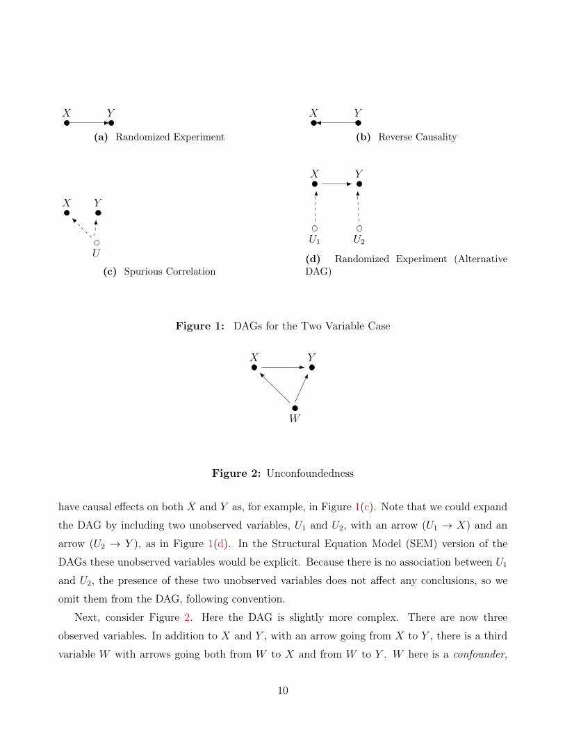
Next, consider Figure 2. Here the DAG is slightly more complex. There are now three
observed variables. In addition to X and Y , with an arrow going from X to Y , there is a third
variable W with arrows going both from W to X and from W to Y . W here is a confounder,
10

X Y
U
Z
Figure 3: Instrumental Variables
or, more precisely, an observed confounder. Simply looking at the association between X and Y
is not sufficient for infering the causal effect: the effect is confounded by the effect of W on X
and Y . Nevertheless, because we observe the confounder W we can still infer the causal effect
of X on Y by controlling or adjusting for W .
Figure 3 is even more complex. Now there are three observed variables, X, Y , and Z,
and one unobserved variable U (denoted by a circle rather than a dot). There are arrows
from Z to X, from X to Y , and from U to both X and Y . The latter two are dashed lines
in the figure to indicate they are between two nodes at least one of which is an unobserved
variable. U is an unobserved confounder. The presence of U makes it in general impossible to
completely infer the average causal effect of X on Y from just the joint distribution of X and Y ,
although bounds as in [Manski, 1990]. The presence of the additional variable, the instrument
Z, is one way to make progress. This DAG captures an instrumental variables setting. In the
econometrics terminology X is endogenous because there is an unobserved confounder U that
affects both X and Y . There is no direct effect of the instrument Z on the outcome Y , and there
is no unobserved confounder for the effect of the instrument on the endogenous regressor or the
outcome. This instrumental variables set up is familiar to economists, although traditionally in a
non-DAG form. In support of his first argument of the benefits of DAGs, TBOW argues that the
DAG version clarifies the key assumptions and structure compared to the econometrics set up.
Compared to the traditional econometrics setup where the critical assumptions are expressed in
terms of the correlation between residuals and instruments, I agree with TBOW that the DAGs
are superior in clarity. I am less convinced of the benefits of the DAG relative to the modern
PO set up for the IV setting with its separation of the critical assumptions into design-based
11
Z0
Z1
B
Z2
X Z3
Y
(a) original
Z0
Z1
B
Z2
X Z3
Y
(b) Two Additional Links
Figure 4: Based on Figure 1 in [Pearl, 1995].
unconfoundedness assumptions and a substantive exclusion restriction (e.g., [Angrist, Imbens,
and Rubin, 1996]), but that appears to me to be a matter of taste. Certainly for many people the
DAGs are an effective expository tool. That is quite separate from its value as formal method for
infering identification and lack thereof. Note that formally in this instrumental variables setting
identification of the average causal effect of X on Y is a subtle one, and in fact this average
effect is not identified according to the DAG methodology. I will return to this setting where
only the Local Average Treatment Effect (LATE) is identified ([Imbens and Angrist, 1994]) in
more detail in Section 4.2. It is an important example because it shows explicitly the inability
of the DAGs to derive some classes of identification results.
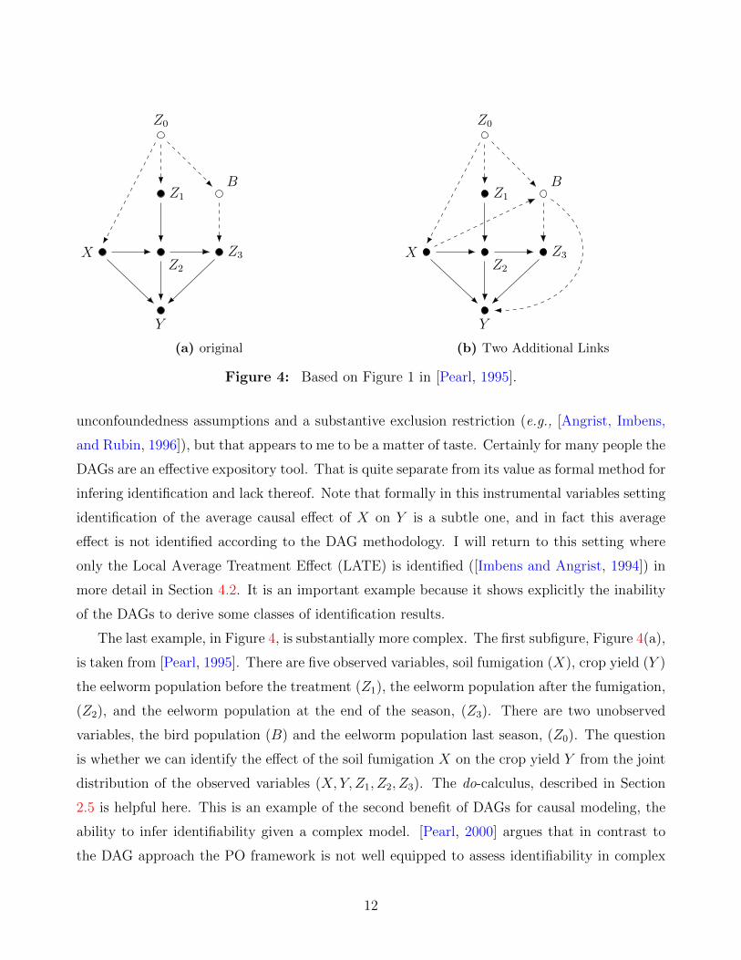
The last example, in Figure 4, is substantially more complex. The first subfigure, Figure 4(a),
is taken from [Pearl, 1995]. There are five observed variables, soil fumigation (X), crop yield (Y )
the eelworm population before the treatment (Z1), the eelworm population after the fumigation,
(Z2), and the eelworm population at the end of the season, (Z3). There are two unobserved
variables, the bird population (B) and the eelworm population last season, (Z0). The question
is whether we can identify the effect of the soil fumigation X on the crop yield Y from the joint
distribution of the observed variables (X, Y, Z1, Z2, Z3). The do-calculus, described in Section
2.5 is helpful here. This is an example of the second benefit of DAGs for causal modeling, the
ability to infer identifiability given a complex model. [Pearl, 2000] argues that in contrast to
the DAG approach the PO framework is not well equipped to assess identifiability in complex
12
models involving a large number of variables:
“no mortal can apply this condition [ignorability, GWI] to judge whether it holds
even in simple problems, with all causal relationships correctly specified, let alone
in partially specified problems that involve dozens of variables.” ([Pearl, 2000], p.
350).
Similarly, Elias Bareinboim writes,
“Regarding the frontdoor or napkin, these are just toy examples where the cur-
rent language [the PO framework, GWI] has a hard time solving, I personally never
saw a natural solution. If this happens with 3, 4 var examples, how could some-
one solve one 100-var instance compounded with other issues?” (Elias Bareinboim,
Twitter,@eliasbareinboim, March 17, 2019).
I agree that in cases like this inferring identifiability is a challenge that few economists would be
equipped to meet. However, in modern empirical work in economics there are few cases where
researchers consider models with dozens, let alone a hundred, variables and complex relations
between them that do not reduce to simple identification strategies. As Jason Abaluck responds
to Bareinboim’s comment:
“No one should ever write down a 100 variable DAG and do inference based on
that. That would be an insane approach because the analysis would be totally
impenetrable. Develop a research design where that 100 variable DAG trivially
reduces to a familiar problem (e.g. IV!)” (Jason Abaluck, Twitter, @abaluck, March
17th, 2019).
Many years ago [Leamer, 1983] in his classic paper “Let’s take the Con out of Econometrics,”
articulated this suspicion of models that rely on complex structures between a large number of
variables most eloquently (and curiously also in the context of studying the effect of fertilizer
on crop yields):
“ The applied econometrician is like a farmer who notices that the yield is somewhat
higher under trees where birds roost, and he uses this as evidence that bird droppings
increase yields. However, when he presents this finding at the annual meeting of the
American Ecological Association, another farmer in the audience objects that he
13
used the same data but came up with the conclusion that moderate amounts of
shade increase yields. A bright chap in the back of the room then observes that
these two hypotheses are indistinguishable, given the available data. He mentions
the phrase ”identification problem,” which, though no one knows quite what he
means, is said with such authority that it is totally convincing.” ([Leamer, 1983], p.
31).
Ultimately Leamer’s concerns were part of what led to the credibility revolution ([Angrist and
Pischke, 2010]) with its focus on credible identification strategies, typically in settings with
a modest number (of sets) of variables. This is why much of the training in economics PhD
programs attempts to provide economists with a deep understanding of a number of the identifi-
cation strategies listed earlier, regression discontinuity designs, instrumental variables, synthetic
controls, unconfoundedness, and others, including the statistical methods appropriate for each
of these identification strategy, than train them to be able to infer identification in complex,
and arguably implausible, models. That is not to say that there is not an important role for
structural modeling in econometrics. However, the structural models used in econometrics use
economic theory more deeply than the current DAGs, exploiting monotonicity and other shape
restrictions as well as other implications of the theory that are not easily incorporated in the
DAGs and the attendant do-calculus, despite the claims of universality of the DAGs.
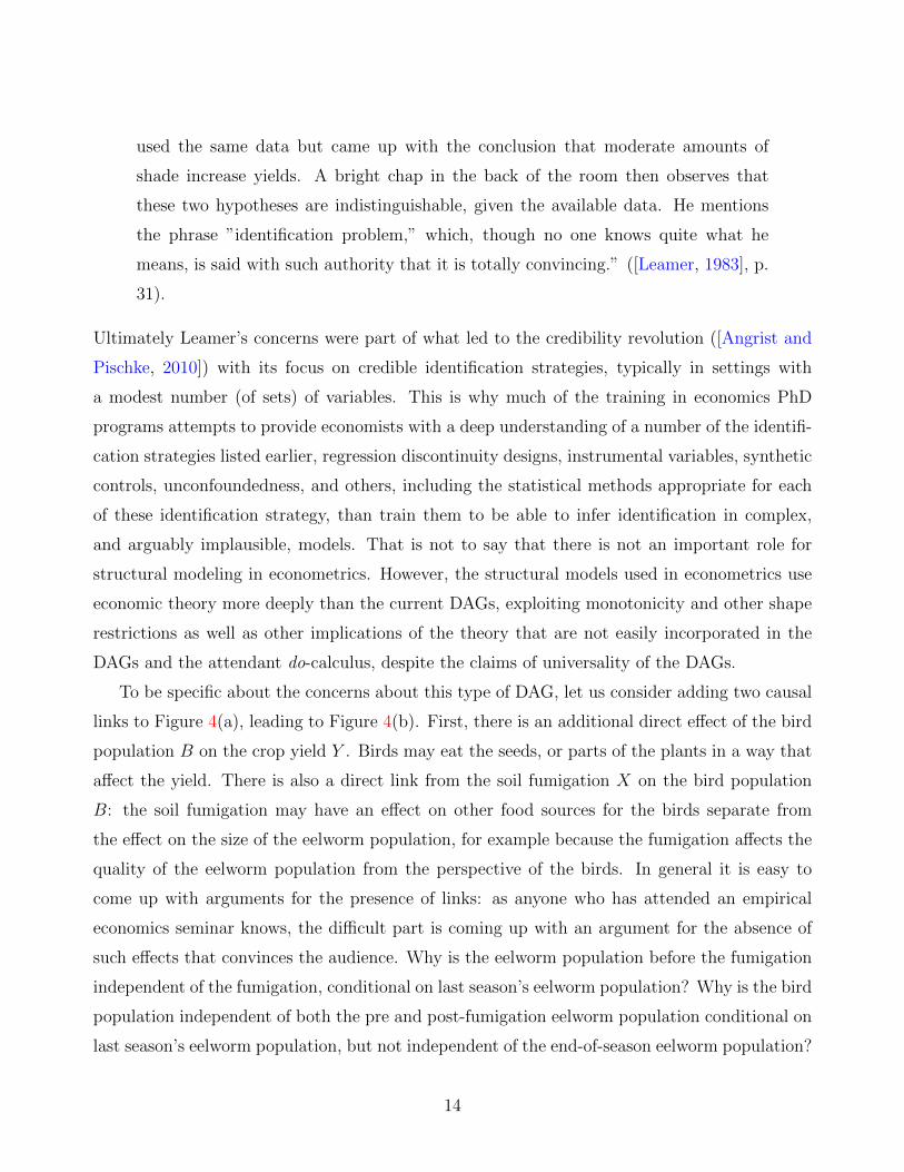
To be specific about the concerns about this type of DAG, let us consider adding two causal
links to Figure 4(a), leading to Figure 4(b). First, there is an additional direct effect of the bird
population B on the crop yield Y . Birds may eat the seeds, or parts of the plants in a way that
affect the yield. There is also a direct link from the soil fumigation X on the bird population
B: the soil fumigation may have an effect on other food sources for the birds separate from
the effect on the size of the eelworm population, for example because the fumigation affects the
quality of the eelworm population from the perspective of the birds. In general it is easy to
come up with arguments for the presence of links: as anyone who has attended an empirical
economics seminar knows, the difficult part is coming up with an argument for the absence of
such effects that convinces the audience. Why is the eelworm population before the fumigation
independent of the fumigation, conditional on last season’s eelworm population? Why is the bird
population independent of both the pre and post-fumigation eelworm population conditional on
last season’s eelworm population, but not independent of the end-of-season eelworm population?
14

This difficulty in arguing for the absence of effects is particularly true in social sciences where
any effects that can possibly be there typically are, in comparison with physical sciences where
the absence of deliberate behavior may enable the researcher to rule out particular causal links.
As Gelman puts it, “More generally, anything that plausibly could have an effect will not have
an effect that is exactly zero.” ([Gelman, 2011], p. 961). Another question regarding the specific
DAG here is why the size of the eelworm population is allowed to change repeatedly, whereas
the local bird population remains fixed.
The point of this discussion is that a major challenge in causal inference is coming up with the
causal model or DAG. Establishing whether a particular model is identified, and if so, whether
there are testable restrictions, in other words, the parts that a DAG is potentially helpful for,
is a secondary, and much easier, challenge.
2.4 Some DAG Terminology
Let me now introduce some additional terminology to facilitate the discussion. See TBOW or
[Pearl, 2000] for details. To make the concepts specific I will focus on the eelworm example
from Figure 4(a). The set of nodes in this DAG is Z = {Z0, Z1, Z2, Z3, B,X, Y }. The edges are
Z0 → X, Z0 → Z1, Z0 → B, Z1 → Z2, B → Z3, X → Y , X → Z2, Z2 → Z3, Z2 → Y , and
Z3 → Y . Consider a node in this DAG. For any given node, all the nodes that have arrows going
directly into that node are its parents. In Figure 4(a), for example, X and Z1 are the parents
of Z2. Ancestors of a node include parents of that node, their parents, and so on. The full set
of ancestors of Z2 is {Z0, Z1, X}. For any given node all the nodes that have arrows going into
them directly from the given node are its children. In Figure 4(a) Z2 is the only child of Z1.
Descendants of a node include its children, their children, and so on. The set of descendants of
Z1 is {Z2, Z3, Y }.A path between two different nodes is a set of connected edges starting from the first node
going to the second node, irrespective of the direction of the arrows. For example, one path
going from Z2 to Z3 is the edge (Z2 → Z3). Another path is (Z2 ← X → Y ← Z3). A collider
of a path is an non-endpoint node on that path with arrows from that path going into the
node, but no arrows from that path emerging from that node. Z2 is a collider on the path
(X → Z2 ← Z1). Note that a node X can be a collider on one path from Z to Y and the same
node can be a non-collider on a different path from Z to Y , so that clearly being a collider is
15
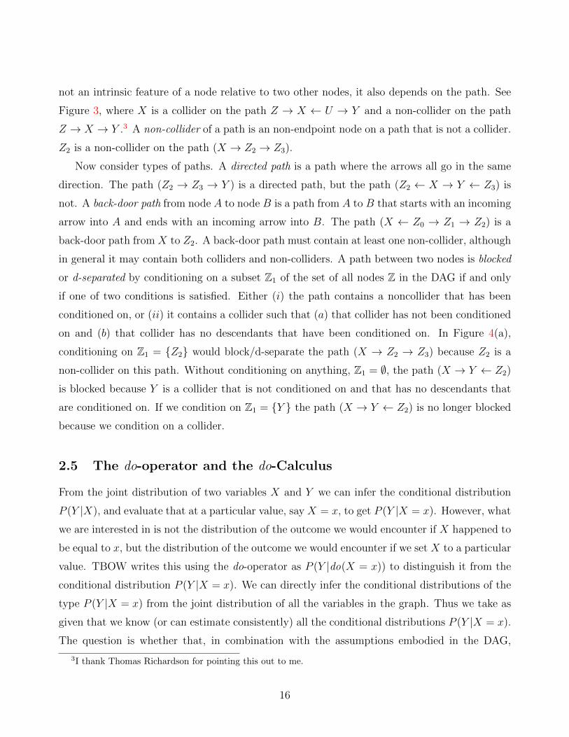
not an intrinsic feature of a node relative to two other nodes, it also depends on the path. See
Figure 3, where X is a collider on the path Z → X ← U → Y and a non-collider on the path
Z → X → Y .3 A non-collider of a path is an non-endpoint node on a path that is not a collider.
Z2 is a non-collider on the path (X → Z2 → Z3).
Now consider types of paths. A directed path is a path where the arrows all go in the same
direction. The path (Z2 → Z3 → Y ) is a directed path, but the path (Z2 ← X → Y ← Z3) is
not. A back-door path from node A to node B is a path from A to B that starts with an incoming
arrow into A and ends with an incoming arrow into B. The path (X ← Z0 → Z1 → Z2) is a
back-door path from X to Z2. A back-door path must contain at least one non-collider, although
in general it may contain both colliders and non-colliders. A path between two nodes is blocked
or d-separated by conditioning on a subset Z1 of the set of all nodes Z in the DAG if and only
if one of two conditions is satisfied. Either (i) the path contains a noncollider that has been
conditioned on, or (ii) it contains a collider such that (a) that collider has not been conditioned
on and (b) that collider has no descendants that have been conditioned on. In Figure 4(a),
conditioning on Z1 = {Z2} would block/d-separate the path (X → Z2 → Z3) because Z2 is a
non-collider on this path. Without conditioning on anything, Z1 = ∅, the path (X → Y ← Z2)
is blocked because Y is a collider that is not conditioned on and that has no descendants that
are conditioned on. If we condition on Z1 = {Y } the path (X → Y ← Z2) is no longer blocked
because we condition on a collider.
2.5 The do-operator and the do-Calculus
From the joint distribution of two variables X and Y we can infer the conditional distribution
P (Y |X), and evaluate that at a particular value, say X = x, to get P (Y |X = x). However, what
we are interested in is not the distribution of the outcome we would encounter if X happened to
be equal to x, but the distribution of the outcome we would encounter if we set X to a particular
value. TBOW writes this using the do-operator as P (Y |do(X = x)) to distinguish it from the
conditional distribution P (Y |X = x). We can directly infer the conditional distributions of the
type P (Y |X = x) from the joint distribution of all the variables in the graph. Thus we take as
given that we know (or can estimate consistently) all the conditional distributions P (Y |X = x).
The question is whether that, in combination with the assumptions embodied in the DAG,
3I thank Thomas Richardson for pointing this out to me.
16
allows us to infer causal objects of the type P (Y |do(X = x)). This is what the do-calculus is
intended to do. See Tucci [2013] and TBWO for accessible introductions, and [Pearl, 1995, 2000]
for more details.
How does the do-calculus relate to the DAG? Suppose we are interested in the causal effect
of X on Y . This corresponds to comparing P (Y |do(X = x)) for different values of x. To
obtain P (Y |do(X)) we modify the graph in a specific way (we perform surgery on the graph),
using the do-calculus. Specifically, we remove all the arrows going into X. This gives us a new
causal model. For that new model the distribution P (Y |X) is the same as P (Y |do(X)). So,
the question is how we infer P (Y |X) in the new post-surgery model from the joint distribution
of all the observed variables in the old pre-surgery model. One tool is to condition on certain
variables. Instead of looking at the correlation between two variables Y and X, we may look at
the conditional correlation between them where we condition on a set of additional variables.
Whether the conditioning works to obtain the causal effects is one of the key questions that the
DAGs are intended to answer.
The do-calculus has three fundamental rules. Here we use the versions in TBOW, which are
slightly different from those in [Pearl, 2000]:
1. Consider a DAG, and P (Y |do(X), Z,W ). If, after deleting all paths into X, the set of
variables Z blocks all the paths from W to Y , then P (Y |do(X), Z,W ) = P (Y |do(X), Z).
2. If a set of variables Z blocks all back-door paths from X to Y , then P (Y |do(X), Z) =
P (Y |X,Z) (“doing” X is the same as “seeing” X).
3. If there is no path from X to Y with only forward-directed arrows, then P (Y |do(X)) =
P (Y ).
Let us consider two of the most important examples of identification strategies based on
the do-calculus for identifying causal effects in DAG, the back-door criterion and the front-door
criterion.
2.6 The Back-door Criterion
The back-door criterion for identifying the causal effect of a node X on a node Y is based on
blocking all backdoor paths through conditioning on a subset of nodes. Let us call this subset of
17

conditioning variables Zbd, where the subscript “bd” stands for back-door. When is it sufficient
to condition on this subset? We need to check whether all back-door paths are blocked as a
result of conditioning on Zbd. Recall the definition of blocking or d-separating a backdoor path.
It requires either conditioning on a non-collider, or the combination of not conditioning on a
collider and not conditioning on all the descendants of that collider.
Consider Figure 2. In this case conditioning on Zbd = {W} suffices. By the second rule
of the do-calculus, P (Y |do(x),W ) = P (Y |X = x,W ) and so P (Y |do(x)) can be inferred from
P (Y |X = x,W ) by integrating over the marginal distribution of W . In Figure 3, however,
the backdoor criterion does not work. There is a backdoor path from X to Y that cannot be
blocked, namely the path (X ← U → Y ). We cannot block the path by conditioning on U
because U is not observed.
The back-door criterion typically leads to the familiar type of statistical adjustments through
matching, weighting, regression adjustments, or doubly-robust methods (see [Imbens, 2004,
Abadie and Cattaneo, 2018] for surveys). The main difference is that given the DAG it provides
a criterion for selecting the set of variables to condition on.
2.7 The Front-door Criterion
A second identification strategy is the front-door criterion. This strategy for identifying the
effect of a variable X on an outcome Y does not rely on blocking all back-door paths. Instead
the front-door criterion relies on the existence of intermediate variables that lie on the causal
path from X to Y . It relies both on the effect of X on these intermediate variables being
identified, and on the effect of the intermediate variables on the outcome being identified. This
is an interesting strategy in the sense that it is not commonly seen in economics.
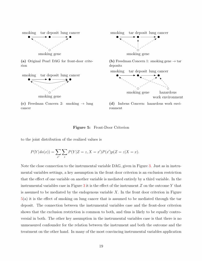
Consider the DAG in Figure 5(a) using a widely used example of the front-door criterion.
We are interested in the causal effect of smoking (X) on lung cancer (Y ). A smoking gene (U)
is an unobserved confounder for this causal effect, so P (Y |X) 6= P (Y |do(X)). However, there
is another way to identify the causal effect of interest, using the additional variable tar deposits
(Z). We can identify the causal effect of X on Z because there is no unobserved confounder,
and P (Z|X) = P (Z|do(X)). We can identify the causal effect of Z on Y by adjusting for X,
because P (Y |Z,X) = P (Y |do(Z), X). Putting these two together allows us to infer the causal
effect of X on Y . With discrete Z, the formula that relates the average causal effect of X on Y
18
smoking tar deposit
smoking gene
lung cancer
(a) Original Pearl DAG for front-door crite-rion
smoking tar deposit
smoking gene
lung cancer
(b) Freedman Concern 1: smoking gene→ tardeposits
smoking tar deposit
smoking gene
lung cancer
(c) Freedman Concern 2: smoking → lungcancer
smoking tar deposit
smoking gene
lung cancer
hazardouswork environment
(d) Imbens Concern: hazardous work envi-ronment
Figure 5: Front-Door Criterion
to the joint distribution of the realized values is
P (Y |do(x)) =∑x′
∑z
P (Y |Z = z,X = x′)P (x′)p(Z = z|X = x).
Note the close connection to the instrumental variable DAG, given in Figure 3. Just as in instru-
mental variables settings, a key assumption in the front door criterion is an exclusion restriction
that the effect of one variable on another variable is mediated entirely by a third variable. In the
instrumental variables case in Figure 3 it is the effect of the instrument Z on the outcome Y that
is assumed to be mediated by the endogenous variable X. In the front door criterion in Figure
5(a) it is the effect of smoking on lung cancer that is assumed to be mediated through the tar
deposit. The connection between the instrumental variables case and the front-door criterion
shows that the exclusion restriction is common to both, and thus is likely to be equally contro-
versial in both. The other key assumption in the instrumental variables case is that there is no
unmeasured confounder for the relation between the instrument and both the outcome and the
treatment on the other hand. In many of the most convincing instrumental variables application
19

that assumption is satisfied by design because of randomization of the instrument (e.g, the draft
lottery number in [Angrist, 1990], and random assignment in randomized controlled trials with
noncompliance, [Hirano, Imbens, Rubin, and Zhou, 2000]). In the front door case the additional
key assumption is that there are no unmeasured confounders for the intermediate variable and
the outcome. Unlike the no-unmeasured-confounder assumption in the instrumental variables
case this assumption cannot be guaranteed by design. As a result it will be controversial in
many applications.
The front-door criterion is an interesting case, and in some sense an important setting for
the DAGs versus PO discussion. I am not aware of any applications in economics that explic-
itly use this identification strategy. The question arises whether this is an important method,
whose omission from the canon of identification strategies has led economists to miss interesting
opportunities to identify causal effects. If so, one might argue that is should be added to the
canon along side instrumental variables, regression discontinuity designs and others. TBOW
clearly think so, and are very high on this identification strategy:
“[the front door criterion] allows us to control for confounders that we cannot observe
... including those we can’t even name. RCTs [Randomized Controlled Trials, GWI]
are considered the gold standard of causal effect estimation for exactly the same
reason. Because front-door estimates do the same thing, with the additional virtue
of observing people’s behavior in their own natural habitat instead of a laboratory,
I would not be surprised if this method eventually becomes a serious competitor to
randomized controlled trials.” (TBOW, p. 231).
David Cox and Nanny Wermuth on the other hand are not quite convinced, and, in a comment
on [Pearl, 1995] write:
“Moreover, an unobserved variable U affecting both X and Y must have no direct
effect on Z. Situations where this could be assumed with any confidence seem likely
to be exceptional.” ([Cox and Wermuth, 1995], p. 689).
As the Cox-Wermuth quote suggests, a question that does not get answered in many discussions
of the front-door criterion is how credible the strategy is in practice. The smoking and lung
cancer example TBOW uses has been used in a number of other studies as well, e.g., [Koller,
Friedman, and Bach, 2009]. TBOW mentions that the former Berkeley statistician David Freed-
man raised three concerns regarding the DAG in Figure 5(a). He thought the same unobserved
20
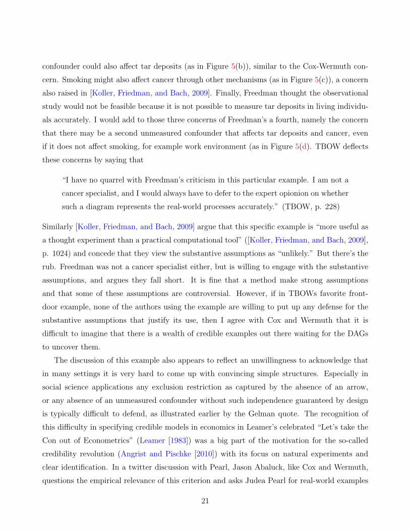
confounder could also affect tar deposits (as in Figure 5(b)), similar to the Cox-Wermuth con-
cern. Smoking might also affect cancer through other mechanisms (as in Figure 5(c)), a concern
also raised in [Koller, Friedman, and Bach, 2009]. Finally, Freedman thought the observational
study would not be feasible because it is not possible to measure tar deposits in living individu-
als accurately. I would add to those three concerns of Freedman’s a fourth, namely the concern
that there may be a second unmeasured confounder that affects tar deposits and cancer, even
if it does not affect smoking, for example work environment (as in Figure 5(d). TBOW deflects
these concerns by saying that
“I have no quarrel with Freedman’s criticism in this particular example. I am not a
cancer specialist, and I would always have to defer to the expert opionion on whether
such a diagram represents the real-world processes accurately.” (TBOW, p. 228)
Similarly [Koller, Friedman, and Bach, 2009] argue that this specific example is “more useful as
a thought experiment than a practical computational tool” ([Koller, Friedman, and Bach, 2009],
p. 1024) and concede that they view the substantive assumptions as “unlikely.” But there’s the
rub. Freedman was not a cancer specialist either, but is willing to engage with the substantive
assumptions, and argues they fall short. It is fine that a method make strong assumptions
and that some of these assumptions are controversial. However, if in TBOWs favorite front-
door example, none of the authors using the example are willing to put up any defense for the
substantive assumptions that justify its use, then I agree with Cox and Wermuth that it is
difficult to imagine that there is a wealth of credible examples out there waiting for the DAGs
to uncover them.
The discussion of this example also appears to reflect an unwillingness to acknowledge that
in many settings it is very hard to come up with convincing simple structures. Especially in
social science applications any exclusion restriction as captured by the absence of an arrow,
or any absence of an unmeasured confounder without such independence guaranteed by design
is typically difficult to defend, as illustrated earlier by the Gelman quote. The recognition of
this difficulty in specifying credible models in economics in Leamer’s celebrated “Let’s take the
Con out of Econometrics” (Leamer [1983]) was a big part of the motivation for the so-called
credibility revolution (Angrist and Pischke [2010]) with its focus on natural experiments and
clear identification. In a twitter discussion with Pearl, Jason Abaluck, like Cox and Wermuth,
questions the empirical relevance of this criterion and asks Judea Pearl for real-world examples
21
W Z X Y
U2
U1
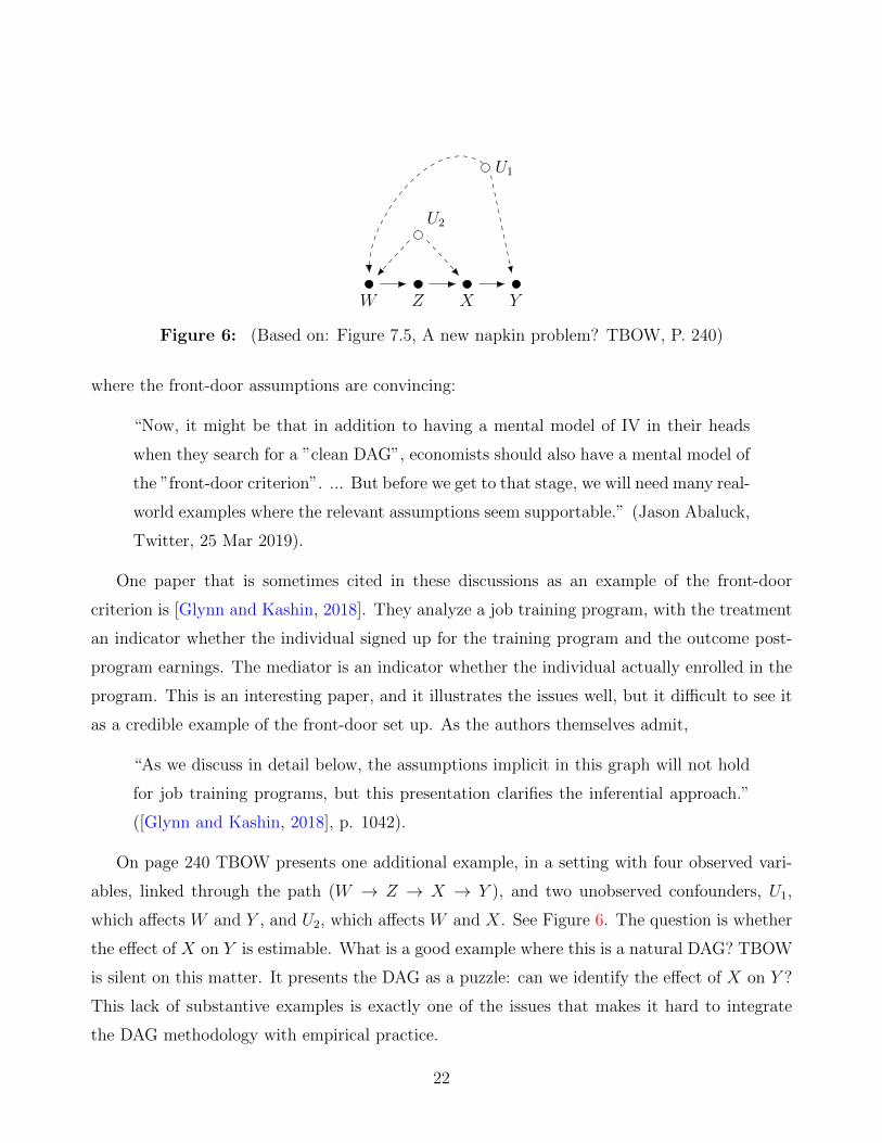
Figure 6: (Based on: Figure 7.5, A new napkin problem? TBOW, P. 240)
where the front-door assumptions are convincing:
“Now, it might be that in addition to having a mental model of IV in their heads
when they search for a ”clean DAG”, economists should also have a mental model of
the ”front-door criterion”. ... But before we get to that stage, we will need many real-
world examples where the relevant assumptions seem supportable.” (Jason Abaluck,
Twitter, 25 Mar 2019).
One paper that is sometimes cited in these discussions as an example of the front-door
criterion is [Glynn and Kashin, 2018]. They analyze a job training program, with the treatment
an indicator whether the individual signed up for the training program and the outcome post-
program earnings. The mediator is an indicator whether the individual actually enrolled in the
program. This is an interesting paper, and it illustrates the issues well, but it difficult to see it
as a credible example of the front-door set up. As the authors themselves admit,
“As we discuss in detail below, the assumptions implicit in this graph will not hold
for job training programs, but this presentation clarifies the inferential approach.”
([Glynn and Kashin, 2018], p. 1042).
On page 240 TBOW presents one additional example, in a setting with four observed vari-
ables, linked through the path (W → Z → X → Y ), and two unobserved confounders, U1,
which affects W and Y , and U2, which affects W and X. See Figure 6. The question is whether
the effect of X on Y is estimable. What is a good example where this is a natural DAG? TBOW
is silent on this matter. It presents the DAG as a puzzle: can we identify the effect of X on Y ?
This lack of substantive examples is exactly one of the issues that makes it hard to integrate
the DAG methodology with empirical practice.
22
X S
W
Y
(a) Mediation
X S
W
Y
(b) Surrogates
X S
W
Y
U
(c) Invalid Surrogates
X S
W
Y
U
(d) Invalid Surrogates
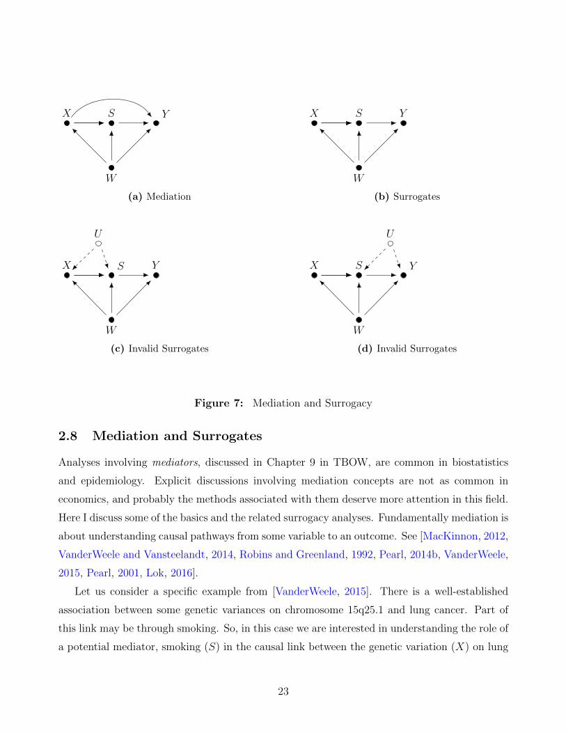
Figure 7: Mediation and Surrogacy
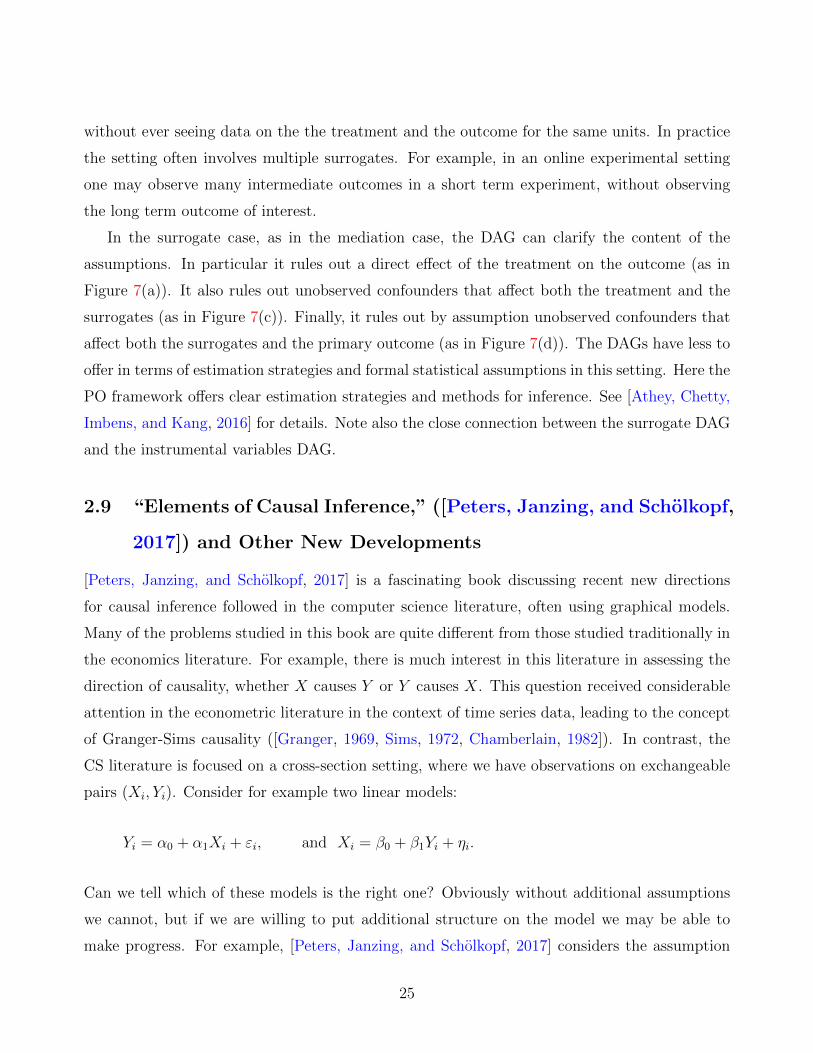
2.8 Mediation and Surrogates
Analyses involving mediators, discussed in Chapter 9 in TBOW, are common in biostatistics
and epidemiology. Explicit discussions involving mediation concepts are not as common in
economics, and probably the methods associated with them deserve more attention in this field.
Here I discuss some of the basics and the related surrogacy analyses. Fundamentally mediation is
about understanding causal pathways from some variable to an outcome. See [MacKinnon, 2012,
VanderWeele and Vansteelandt, 2014, Robins and Greenland, 1992, Pearl, 2014b, VanderWeele,
2015, Pearl, 2001, Lok, 2016].
Let us consider a specific example from [VanderWeele, 2015]. There is a well-established
association between some genetic variances on chromosome 15q25.1 and lung cancer. Part of
this link may be through smoking. So, in this case we are interested in understanding the role of
a potential mediator, smoking (S) in the causal link between the genetic variation (X) on lung
23
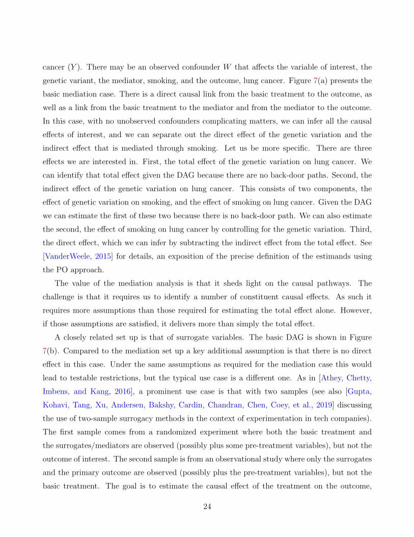
cancer (Y ). There may be an observed confounder W that affects the variable of interest, the
genetic variant, the mediator, smoking, and the outcome, lung cancer. Figure 7(a) presents the
basic mediation case. There is a direct causal link from the basic treatment to the outcome, as
well as a link from the basic treatment to the mediator and from the mediator to the outcome.
In this case, with no unobserved confounders complicating matters, we can infer all the causal
effects of interest, and we can separate out the direct effect of the genetic variation and the
indirect effect that is mediated through smoking. Let us be more specific. There are three
effects we are interested in. First, the total effect of the genetic variation on lung cancer. We
can identify that total effect given the DAG because there are no back-door paths. Second, the
indirect effect of the genetic variation on lung cancer. This consists of two components, the
effect of genetic variation on smoking, and the effect of smoking on lung cancer. Given the DAG
we can estimate the first of these two because there is no back-door path. We can also estimate
the second, the effect of smoking on lung cancer by controlling for the genetic variation. Third,
the direct effect, which we can infer by subtracting the indirect effect from the total effect. See
[VanderWeele, 2015] for details, an exposition of the precise definition of the estimands using
the PO approach.
The value of the mediation analysis is that it sheds light on the causal pathways. The
challenge is that it requires us to identify a number of constituent causal effects. As such it
requires more assumptions than those required for estimating the total effect alone. However,
if those assumptions are satisfied, it delivers more than simply the total effect.
A closely related set up is that of surrogate variables. The basic DAG is shown in Figure
7(b). Compared to the mediation set up a key additional assumption is that there is no direct
effect in this case. Under the same assumptions as required for the mediation case this would
lead to testable restrictions, but the typical use case is a different one. As in [Athey, Chetty,
Imbens, and Kang, 2016], a prominent use case is that with two samples (see also [Gupta,
Kohavi, Tang, Xu, Andersen, Bakshy, Cardin, Chandran, Chen, Coey, et al., 2019] discussing
the use of two-sample surrogacy methods in the context of experimentation in tech companies).
The first sample comes from a randomized experiment where both the basic treatment and
the surrogates/mediators are observed (possibly plus some pre-treatment variables), but not the
outcome of interest. The second sample is from an observational study where only the surrogates
and the primary outcome are observed (possibly plus the pre-treatment variables), but not the
basic treatment. The goal is to estimate the causal effect of the treatment on the outcome,
24
without ever seeing data on the the treatment and the outcome for the same units. In practice
the setting often involves multiple surrogates. For example, in an online experimental setting
one may observe many intermediate outcomes in a short term experiment, without observing
the long term outcome of interest.
In the surrogate case, as in the mediation case, the DAG can clarify the content of the
assumptions. In particular it rules out a direct effect of the treatment on the outcome (as in
Figure 7(a)). It also rules out unobserved confounders that affect both the treatment and the
surrogates (as in Figure 7(c)). Finally, it rules out by assumption unobserved confounders that
affect both the surrogates and the primary outcome (as in Figure 7(d)). The DAGs have less to
offer in terms of estimation strategies and formal statistical assumptions in this setting. Here the
PO framework offers clear estimation strategies and methods for inference. See [Athey, Chetty,
Imbens, and Kang, 2016] for details. Note also the close connection between the surrogate DAG
and the instrumental variables DAG.
2.9 “Elements of Causal Inference,” ([Peters, Janzing, and Scholkopf,
2017]) and Other New Developments
[Peters, Janzing, and Scholkopf, 2017] is a fascinating book discussing recent new directions
for causal inference followed in the computer science literature, often using graphical models.
Many of the problems studied in this book are quite different from those studied traditionally in
the economics literature. For example, there is much interest in this literature in assessing the
direction of causality, whether X causes Y or Y causes X. This question received considerable
attention in the econometric literature in the context of time series data, leading to the concept
of Granger-Sims causality ([Granger, 1969, Sims, 1972, Chamberlain, 1982]). In contrast, the
CS literature is focused on a cross-section setting, where we have observations on exchangeable
pairs (Xi, Yi). Consider for example two linear models:
Yi = α0 + α1Xi + εi, and Xi = β0 + β1Yi + ηi.
Can we tell which of these models is the right one? Obviously without additional assumptions
we cannot, but if we are willing to put additional structure on the model we may be able to
make progress. For example, [Peters, Janzing, and Scholkopf, 2017] considers the assumption
25
that the unobserved term (εi or ηi) is independent of the right-hand side variable. This is still
not sufficient for choosing between the models if the distributions are Gaussian, but outside of
that, we can now tell the models apart. Identifying models based on this type of functional
form and distributional assumption is not common in economics. The basic question is also
an unusual one in economics settings. In many economic settings we know the cause and the
outcome, that is, we know the direction of the causality, the questions are primarily about
the magnitude of the causal effects, and the possible presence of unmeasured confounders. For
example we are interested in the effect of education on earnings, not the effect of earnings on
education because we know which comes first. In cases where we are unsure about the direction
of the causality there is typically more structure on the problem as well, in terms of mechanisms
involving expectations and feedback loops so that the researcher is not simply trying to infer
from a data set on (Xi, Yi) the direction of the causality.
This example shows how the questions studied in this literature are different from those in
economics. This is particularly true for the questions on causal discovery ([Uhler, Raskutti,
Buhlmann, Yu, et al., 2013, Glymour, Scheines, and Spirtes, 2014, Hoyer, Janzing, Mooij, Pe-
ters, and Scholkopf, 2009, Lopez-Paz, Nishihara, Chintala, Scholkopf, and Bottou, 2017, Mooij,
Peters, Janzing, Zscheischler, and Scholkopf, 2016, Dubois, Oya, Tyszka, Howard III, Eberhardt,
and Adolphs, 2017]), where the goal is to find causal structure in data, without starting with a
fully specified model. The fact that the questions in this literature are currently quite different
from those studied in economics does not take away from the fact that ultimately the results
in this literature may be very relevant for research in social sciences. The aim in the causal
discovery literature is to infer from complex data directly the causal structure governing these
data. If succesful, this would be very relevant for social science questions, but it is currently not
there yet.
More closely related to the econometric literature is the recent work on invariance and
causality (Peters et al. [2016], Buhlmann [2018]).
3 Potential Outcomes and the Rubin Causal Model
What I refer to here as the PO framework is what [Holland, 1986] calls the Rubin Causal Model.
[Rubin, 1974] is a very clear and non-technical introduction, and [Imbens and Rubin, 2015] is
26
a textbook treatment. It has many antecedents in the econometrics literature, as early as the
1930s and 1940s and it is currently widely used in the empirical economics literature. Here I give
a brief overview. The starting point is a population of units. There are then three components
of the PO approach. First, there is a treatment/cause that can take on different values for each
unit. Each unit in the population is characterized by a set of potential outcomes Y (x), one for
each level of the treatment. In the simplest case with a binary treatment there are two potential
outcomes, Y (0) and Y (1), but in other cases there can be more. Only one of these potential
outcomes can be observed, namely the one corresponding to the treatment received:
Y obs = Y (X) =∑x
Y (x)1X=x.
The others are ex post counterfactuals. The causal effects correspond to comparisons of the
potential outcomes, of which at most one can be observed, with all the others missing. Paul
Holland refers to this as the “fundamental problem of causal inference,” ([Holland, 1986], p.
59). This leads to the second component, the presence of multiple units so that we can see
units receiving each of the variour treatments. The third key component is the assignment
mechanism that determines which units receive which treatments. Much of the literature has
concentrated on the case with just a single binary treatment, with the focus on estimating the
average treatment effect of this binary treatment for the entire population or some subpopulation
τ = E[Yi(1)− Yi(0)].
In the do-calculus, this would be written as τ = E[Y (do(1)fs) − Y (do(0))]. At this stage the
difference between the PO and DAG approach is relatively minor. The disctinction between
P (Y |X = x) and P (Y |do(x)) in the PO framework corresponds to the difference between
P (Y obs|X = x) and P (Y (x)). There is a smaller literature on the case with discrete or continuous
treatments (e.g., [Imbens, 2000]).
3.1 Potential Outcomes and Econometrics
For each unit, and for each value of the treatment, there is a potential outcome that could
be observed if that unit was exposed to that level of the treatment. We cannot see the set of
27
potential outcomes for a particular unit because each unit can be exposed to at most one level
of the treatment, and only the potential outcome corresponding to that level of the treatment
can ever be observed. With a single unit and a binary treatment, the two potential outcomes
could be labelled Y (0) and Y (1), with the causal effect being a comparison of the two, say,
the difference Y (1) − Y (0). This is a simple, but powerful notion. It has resonated with
the econometrics and empirical economics community partly because it directly connects with
the way economists think about, say, demand and supply functions. The notion of potential
outcomes is very clearly present in the work of Wright, Tinbergen and Haavelmo in the 1930s
and 1940s ([Wright, 1928, Tinbergen, 1930, Haavelmo, 1943]). For example, Tinbergen carefully
distinguishes in his notation between the price as an argument in the supply and demand
function, and the realized equilibrium price:
“Let π be any imaginable price; and call total demand at this price n(π), and total
supply a(π). Then the actual price p is determined by the equation
a(p) = n(p),
so that the actual quantity demanded, or supplied, obeys the condition u = a(p) =
n(p), where u is this actual quantity.‘’ ([Tinbergen, 1930], translated in [Hendry and
Morgan, 1997], p. 233)
Note also that the potential outcomes, here the supply and demand function, are taken as
primitives, in line with much of the economic literature. Similar to Tinbergen, Haavelmo writes:
“Assume that if the group of all consumers in the society were repeatedly furnished
with the total income, or purchasing power, r per year, they would, on the average,
or ‘normally’, spend a total amount u for consumption per year, equal to
u = αr + β,
where α and β are constants. The amount, u actually spent each year might be
different from u.‘’ (italics in original, [Haavelmo, 1943], p. 3)
Some of the clarity of the potential outcomes that is present in [Tinbergen, 1930] and [Haavelmo,
1943] got lost in some of the subsequent econometrics. The Cowles Foundation research which led
28
to the general simultaneous equations set up, modeled only the observed outcomes and dropped
the notation for the potential outcomes. The resurgence of the use of potential outcomes in the
econometric program evaluation literature starting with [Heckman, 1990] and [Manski, 1990]
caught on precisely because of the precursors in the earlier econometric literature.
3.2 The Assignment Mechanism
The second key component of the PO approach is the assignment mechanism. Given the multiple
potential outcomes for a unit, there is only one of these that can be observed, namely the realized
outcome corresponding to the treatment that was received. Critical is how the treatment was
chosen, that is the assignment mechanism, as a function of the pretreatment variables and
the potential outcomes.. In the simplest case, that of a completely randomized experiment,
it is known to the researcher how the treatment was determined. The assignment mechanism
does not depend on the potential outcomes, and it has a known distribution. For this case we
understand the critical analyses well. This can be relaxed by assuming only unconfoundedness,
where the assignment mechanism is free of dependence on the potential outcomes, but can
depend in arbitrary and unknown ways on the pretreatment variables. Again there is a huge
literature with many well-understood methods. See [Imbens, 2004, Imbens and Rubin, 2015,
Rubin, 2006, Abadie and Cattaneo, 2018] for recent reviews. The most complicated case is
where selection is partly on unobservables, and this case has received the most attention in the
econometrics literature because the starting point there is that agents make deliberate choices,
rather than receiving their treatments by chance (Imbens [2014]).
3.3 Multiple Units and Interference
In many analyses researchers assume that there is no interference between units, part of what
Rubin calls SUTVA (stable unit treatment value assumption). This greatly simplifies analyses,
and makes it conceptually easier to separate the questions of identification and estimation.
However, the assumption that there is no interference is in many cases implausible. There is
also a large and growing literature analyzing settings where this assumption is explicitly relaxed.
Within the PO framework this is conceptually straightforward. Key papers include [Manski,
1993, 2013a, Hudgens and Halloran, 2008, Athey, Eckles, and Imbens, 2018a, Aronow, 2012,
29
Aronow and Samii, 2013, Basse, Feller, and Toulis, 2019, Sobel, 2006]. In many of the settings
considered in this literature it is not so clear what the joint distribution is that can be estimated
precisely in large samples. As a result the separation between identification of the distribution
of observed variables and the identification of causal effects that underlies many of the DAG
analyses is no longer so obvious. Recent work using DAGs with interference includes [Ogburn,
VanderWeele, et al., 2014].
3.4 Randomized Experiments and Experimental Design
In the PO literature there is a very special place for randomized experiments. Consider the
simplest such setting, where Nt units out of the population are randomly selected to receive
the treatment and the remaining Nc = N − Nt are assigned to the control group, and where
the no-interference assumption holds. The implication of the experimental design is that the
treatment is independent of the potential outcomes, or
Wi ⊥⊥(Yi(0), Yi(1)
).
This validates simple estimation strategies. For example, it implies that
τ = Y t − Yc, where Y t =1
Nt
∑i:Wi=1
Yi, and Y c =1
Nc
∑i:Wi=0
Yi,
is unbiased for the average treatment effect, and that
1
Nt(Nt − 1)
∑i:Wi=1
(Yi − Y t
)2+
1
Nc(Nc − 1)
∑i:Wi=0
(Yi − Y c
)2,
is a conservative estimator for the variance, originally proposed by [Neyman, 1923/1990].
The primacy of randomized experiments has long resonated with economists, despite the
limited ability to actually do randomization. Since the late 1990s the development economics
literature has embraced the strength of experiments ([Banerjee and Duflo, 2008]), leading to a
huge empirical literature that has had a major influence on policy. [Angrist and Pischke, 2010]
quote [Haavelmo, 1944] as arguing that we should at least have such an experiment in mind,
even if we are not actually going to (be able to) conduct one:
30
“Over 65 years ago, Haavelmo submitted the following complaint to the readers of
Econometrica (1944, p. 14): A design of experiments (a prescription of what the
physicists call a crucial experiment) is an essential appendix to any quantitative
theory. And we usually have some such experiment in mind when we construct the
theories, although–unfortunately–most economists do not describe their design of
experiments explicitly.” ([Angrist and Pischke, 2010], p. 16)
Similarly, the statistics literature is of course full of claims that randomized experiment are the
most credible setting for making causal claims. [Freedman, 2006] for example is unambiguous
about the primacy of RCTs:
“Experiments offer more reliable evidence on causation than observational studies”
([Freedman, 2006], abstract).
When going beyond randomized experiments, researchers in the PO framework often an-
alyze observational studies by viewing them as emulating particular randomized experiments,
and analyzing them as if there was approximately a randomized experiment. The natural ex-
periment and credibility revolution literatures ([Angrist and Pischke, 2010]), and much of the
subsfsequent empirical literature, are focused on finding settings where assignment is as good
as random at least for a subpopulation, using the various identification strategies including
matching, regression discontinuity designs, synthetic control methods, and instrumental vari-
ables. In contrast, the graphical literature is largely silent about experiments, and does not see
them as special. In fact, Pearl proudly proclaims himself a skeptic of any superiority of RCTs.
When Angus Deaton and Nancy Cartwright write “We argue that any special status for RCTs
is unwarranted.” ([Deaton and Cartwright, 2018], page 2), Pearl comments that
“As a veteran skeptic of the supremacy of the RCT, I welcome D&C’s challenge
wholeheartedly.” ([Pearl, 2018a])
If anything the importance of RCTs has increased in recent years, both in academic circles,
as well as outside in the tech companies: “Together these organizations [Airbnb, Amazon,
Booking.com, Facebook, Google, LinkedIn, Lyft, Microsoft, Netflix, Twitter, Uber, Yandex,
and Stanford University, GWI] tested more than one hundred thousand experiment treatments
last year” ([Gupta, Kohavi, Tang, Xu, Andersen, Bakshy, Cardin, Chandran, Chen, Coey,
et al., 2019], p.20). This has spurred a new literature on the design of experiments in complex
31

W1 W2 W3 . . . Wk
X Y
(a) Confoundedness
W1 W2 W3 . . . Wk
X Y
U
(b) Violation of Unconfoundedness
Figure 8: Unconfoundedness with Multiple Observed Confounders
environments. There are now many computer scientists, economists and statisticians working
on complex experimental designs that take account of interference ([Hudgens and Halloran,
2008, Athey, Eckles, and Imbens, 2018a, Aronow, 2012, Aronow and Samii, 2013, Basse, Feller,
and Toulis, 2019], and that use multi-armed bandit methods and other adaptive designs, [Scott,
2010, Dimakopoulou, Athey, and Imbens, 2017, Dimakopoulou, Zhou, Athey, and Imbens, 2018].
Even in the traditional setting of RCTs for medical treatments these issues have led to new and
innovative designs, e.g., [Isakov, Lo, and Montazerhodjat, 2019, Das and Lo, 2017].
3.5 Unconfoundedness
One of the most common settings for estimating treatment effects is that under unconfounded-
ness or ignorable treatment assignment. The key assumption is that given a set of pre-treatment
variables it is assumed that assignment to treatment is independent of the potential outcomes.
Xi ⊥⊥(Yi(0), Yi(1)
) ∣∣∣ Wi.
A DAG representing this set up is given in Figure 8(a).
The DAG here does not include additional links between the pretreatment variable, but the
estimation strategies justified by the DAG as given can allow for arbitrary links between them.
It does rule out the presence of an unobserved confounder, e.g., the variable U in Figure 8(b).
32
Because it is such a canonical setting, the subject of a huge theoretical literature as well as the
basis for a vast empirical literature, it would appear that the form of the assumptions, graphical
or algebraic, would no longer be a concern in practice because researchers understand what is
the issue here, and can move easily between the DAG and the PO form. However, TBOW
questions whether researchers understand these assumptions:
“Unfortunately, I have yet to find a single person who can explain what ignorability
means in a language spoken by those who need to make this assumption or assess
its plausibility in a given problem.” (TBOW, p. 281).
The unconfoundedness assumption implies that the average treatment effect τ = E[Yi(1)−Yi(0)]
can be written in terms of the joint distribution of the observed variables (Yi, Xi,Wi) as
τ = E[Yi(1)− Yi(0)] = E[E[Yi|Xi = 1,Wi]− E[Yi|Xi = 0,Wi]
].
As arguably the most common setting in empirical work for estimating treatment effects, there is
a huge theoretical literature on specific methods for estimating the average effect of the treatment
on the outcome in this case that has closely interacted with the similarly vast empirical literature.
All methods involve adjusting in some fashion for the difference in pretreatment values Wi
between treated and control units. The methods differ in terms of the components of the joint
distribution of the observed variables they focus on. A key paper is [Rosenbaum and Rubin,
1983b], and more generally the papers in [Rubin, 2006]. A key result is that irrespective of
the number of pre-treatment variables, it is sufficient to adjust for differences between treated
and control units in just a scalar function of the pre-treatment variables, the propensity score,
defined as e(w) = pr(Xi = 1|Wi = w). Much of the statistical and econometric literatures have
focused on effective ways of implementing these ideas in statistics and econometrics. Common in
practice is still the simple least squares estimator, but much of the methodological literature has
developed more robust and efficient methods. Some focus on estimating µ(x,w) = E[Yi|Xi =
x,Wi = w] followed by averaging the difference µ(1,Wi)− µ(0,Wi) over the sample distribution
of the pre-treatment variables Wi. Another strand of the literature has focused on inverse
propensity score weighting, with the weight for unit i proportional to (e(Wi)Xi(1−e(Wi))
1−Xi)−1,
where e(w) = pr(Xi = 1|Wi = x) is the propensity score ([Rosenbaum and Rubin, 1983b]). The
current state of the literature is that the most effective and robust methods use estimates of the
33
conditional outcome means as well as estimates of the propensity score, in what is referred to as
doubly robust methods. See [Robins, Rotnitzky, and Zhao, 1994, Imbens and Wooldridge, 2009,
Abadie and Cattaneo, 2018] for surveys.
Recently this literature has focused on the case with a relatively large number of pre-
treatment variables (Chernozhukov et al. [2017], Athey et al. [2018b], Van der Laan and Rose
[2011], Shi et al. [2019]). Overlap issues in covariate distributions, absent in all the the DAG
discussions, become prominent among practical problems ([Crump, Hotz, Imbens, and Mitnik,
2009, D’Amour, Ding, Feller, Lei, and Sekhon, 2017]). In this setting there has been much
interaction with the machine learning literature, focusing on regularization methods that are
effective given the particular causal estimand, rather than effective for prediction purposes. In
this setting simply assuming that one knows or can consistently estimate the joint distribution
of all variables in the model, which is the basis of the discussion in TBOW and [Pearl, 2000],
is not helpful, and the corresponding “statistical vs. causal dichotomy” ([Pearl, 2000], p. 348)
becomes blurred.
3.6 Sensitivity Analyses
The PO framework has been a natural setting for considering violations of the assumptions
required for point identification. For example, starting with an unconfoundedness setting, one
may wish to consider the presence of an unobserved confounder that has some limited effect on
the treatment assignment as well as on the outcome, and assess the sensitivity of the results to
the presence of such confounders ([Rosenbaum and Rubin, 1983a, Imbens, 2003]). More recent
work has taken these sensitivity analyses further, e.g., [Andrews, Gentzkow, and Shapiro, 2017,
Andrews and Oster, 2019].
4 Graphical Models, Potential Outcomes and Empirical
Practice in Economics
Since its inception in the late 1980s and early 1990s the DAG approach to causality has gener-
ated much interest in among others, computer science, epidemiology, and parts of social science
(e.g., in sociology, [Morgan and Winship, 2014]). In epidemiology in particular it has connected
34

well with related work on structural equations models ([Greenland, Pearl, Robins, et al., 1999,
Robins, 1997]). It has not, however, made major inroads into the theoretical econometric or em-
pirical economic literatures, and is absent from most econometric textbooks (e.g., [Wooldridge,
2001] and MHE). Although causal inference broadly defined has a long and prominent tradition
in econometrics, and since the 1990s there has been a sharp increase in work explicitly focused
on this area, this work has relied primarily on the PO framework. There are exceptions to this,
and there are now some discussions of DAGs in the econometric literature (e.g., the discussion
in [Cunningham, 2018]), and some links in the statistics literature ([Richardson et al., 2011, Ma-
linsky et al., 2019]) but these remain the exception. Much of the empirical work in economics
is closer to the PO approach. Pearl has discussed this, but dismissed the possibility that there
are substantive reasons for this:
“Or, are problems in economics different from those in epidemiology? I have ex-
amined the structure of typical problems in the two fields, the number of variables
involved, the types of data available, and the nature of the research questions. The
problems are strikingly similar.” [Pearl, 2014a].
In this part of this essay I will explore this issue further. I think the case for the DAGs is the
strongest in terms of exposition. The DAGs are often clear and accessible ways to expressing
visually some, though not necessarily all, of the key assumptions. It may provide the reader,
even more than the researcher, with an easy way to interpret and assess the overall model. I am
less convinced that the formal identification results are easier to derive in the DAG framework
for the type of problems commonly studied in economics. I see three reasons for that. First, the
DAGs have difficulty coding shape restrictions such as monotonicity and identification results
for subpopulations. Second, the advantages of the formal methods for deriving identification
results with DAGs are most pronounced in complex models with many variables that are not
particularly popular in empirical economics. Third, the PO approach has connected well with
estimation and inference issues. Although the PO approach has largely focused on the problem
of estimating average effects of binary treatments, it has been able to make much progress there,
not just in terms of identification, but also on problems regarding study design, estimation and
inference. On this issue that the PO or Rubin-Causal-Model framework is much more closely
tied to statistics and practical issues in inference, Steve Powell writes in his review of TBOW
that
35
“Donald Rubin offers an alternative framework [the PO framework, GWI], also not
shy of dealing with causality, which is much more fully developed for the needs and
concerns of social scientists in general and evaluators in particular.” ([Powell, 2018],
p. 53)
I will focus in this section on six specific issues. First, I will discuss the role of randomized
experiments and the importance of manipulability. Second, I will discuss instrumental variables,
the importance of shape restrictions in economics. Third, I will discuss the role of simultaneity
in economics. Fourth, I discuss unconfoundedness, M-bias, and the choice of the set of condi-
tioning variables. Fifth, I will discuss the difficulty with counterfactuals. Finally, I will discuss
identification strategies in the context of the returns to education.
4.1 Non-manipulable Causes or Attributes, Hypothetical Experi-
ments, and the Role of the Assignment Mechanism
The PO framework starts by defining the potential outcomes with reference to a manipulation
(e.g., [Imbens and Rubin, 2015], p. 4). In doing so it makes a distinction between attributes
or pre-treatment variables which are fixed for the units in the population, and causes, which
are potentially manipulable. This is related to the connection between causal statements and
randomized experiments. The causes are conceptually tied to, at the very least hypothetical,
experiments. This may appear to be a disadvantage as it leads to difficulties in the PO framework
when making causal statements about such attributes as race or gender. See the discussion in
[Holland, 1986, Granger, 1986]. In the modern causal literature in economics researchers have
often acknowledged this difficulty and focused on causal effects tied to manipulable aspects of
attributes. A seminal example is [Bertrand and Mullainathan, 2004] who study the well-defined
causal effect of manipulation of the perception of race by changing names from Caucasian
sounding to African-American sounding ones, rather than the less well-defined causal effect of
race itself. This view concerning the importance of manipulability is shared in part of the
statistics literature, where David Cox writes,
“In this discussion, only those variables which in the context in question can con-
ceptually be manipulated are eligible to represent causes, i.e., it must make sense,
always in the context in question, that for any individual the causal variable might
36
have been different from the value actually taken. Thus in most situations gender
is not a causal variable but rather an intrinsic property of the individual.” ([Cox,
1992], p. 296).
The advantage of being explicit about which variables are causal and which are not is that on
only needs to consider the determinants (parents in the DAG terminology) of the causes, and
not those of the attributes.
In contrast, Pearl sees no difficulty in defining causal effects for non-manipulable attributes
in a DAG using the do-calculus:
“Another misguided doctrine denies causal character to nonmanipulable variables.”
([Pearl, 2015] p. 172).
This is not simply a matter of impicitly assuming that the effect of such a variable is invariant to
the method in which is it manipulated, and that therefore the articulation of the manipulation
is immaterial. [Pearl, 2018b] admits that the choice of manipulation may in fact matter, but
that this is simply not relevant for the definition of the do-operator, and that the causal effect
is well-defined irrespective of this. [Pearl, 2018b] discusses the third question from Section 2.1,
the effect of obesity, and admits that the effect of changing obesity through exercise, diet or
surgery may be very different, but that nevertheless the causal effect of obesity on mortality,
corresponding to a virtual intervention, very much in the spirit of a strong version of the ceteris
paribus condition, is well defined:
“While it is true that the probability of death will generally depend on whether we
manipulate obesity through diet versus, say, exercise, [...] do(obesity = x) describes
a virtual intervention, by which nature sets obesity to x, independent of diet or
exercise, while keeping every thing else intact, especially the processes that respond
to X.” ([Pearl, 2018b], p. 3).
Although other researchers working on graphical models have taken a different view on the
manipulability issues (e.g., [Richardson and Robins, 2013, Hernan, Hsu, and Healy, 2018]),
Pearl doubles down on his position that tying causal effects to manipulations is not necessary
in his most recent work:
37
“We end with the conclusion that researchers need not distinguish manipulable from
non-manipulable variables; both types are equally eligible to receive the do(x) oper-
ator” ([Pearl, 2019], abstract).
I find the position that the manipulation is irrelevant unsatisfactory, and find the insistence in
the PO approach on a theoretical or practical manipulation helpful. I am not sure what is meant
by do(obesity = x) if the effect of changing obesity depends on the mechanism (say, exercise,
diet, or surgery), and the mechanism is not specified in the operator. It is also not obvious
to me why we would care about the value of do(obesity = x) if the effect is not tied to an
intervention we can envision. The insistence on manipulability in the PO framework resonates
well in economics where policy relevance is a key goal (e.g., [Manski, 2013b]). We are interested
in policies that change the weight for currently obese people (e.g., encouraging exercise, dietary
changes, or surgery), or that discourage currently non-obese people who are at risk of becoming
obese from doing so (exercise, dietary changes, or other life-style changes). What is relevant
for policy makers is the causal effect of such policies, not the effect of a virtual intervention
that makes currently obese people suddenly like non-obese people. In my original 1995 PhD
course with Don Rubin on causal inference we had a similar discussion about the “causal effect
of child poverty.” From our perspective that question was ill-posed, and a better-posed question
would be about the effect of a particular intervention that would make currently poor families
financially better off. One draconian policy to achieve this would be to take the children away
from the poor families and put them with richer families. That does not seem like a policy the
government should or would consider in this day and age. A more interesting policy would be
to provide additional financial resources to currently poor families. The discusion in that class
led to a study of the effect of one such intervention, namely winning the lottery on subsequent
outcomes (which ultimately led to [Imbens, Rubin, and Sacerdote, 2001]) as a way of illustrating
the causal effect of a particular manipulation.
Without a specific manipulation in mind, it is also difficult to assess a particular identification
strategy. It is only in the context of a particular treatment that it becomes clear whether in
the analysis of the effects of obesity diet is a confounder or a mediator, partly dependent on
the relative timing of the intervention. The flip side of that is that if the treatment is a virtual
intervention, it becomes difficult to assess whether there are unobserved confounders.
As a third example to clarify the benefits from being explicit about the nature of the ma-
38
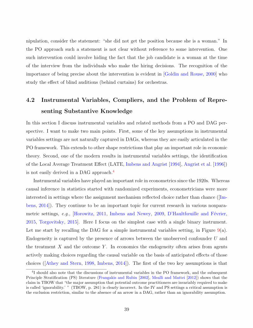
nipulation, consider the statement: “she did not get the position because she is a woman.” In
the PO approach such a statement is not clear without reference to some intervention. One
such intervention could involve hiding the fact that the job candidate is a woman at the time
of the interview from the individuals who make the hiring decisions. The recognition of the
importance of being precise about the intervention is evident in [Goldin and Rouse, 2000] who
study the effect of blind auditions (behind curtains) for orchestras.
4.2 Instrumental Variables, Compliers, and the Problem of Repre-
senting Substantive Knowledge
In this section I discuss instrumental variables and related methods from a PO and DAG per-
spective. I want to make two main points. First, some of the key assumptions in instrumental
variables settings are not naturally captured in DAGs, whereas they are easily articulated in the
PO framework. This extends to other shape restrictions that play an important role in economic
theory. Second, one of the modern results in instrumental variables settings, the identification
of the Local Average Treatment Effect (LATE, Imbens and Angrist [1994], Angrist et al. [1996])
is not easily derived in a DAG approach.4
Instrumental variables have played an important role in econometrics since the 1920s. Whereas
causal inference in statistics started with randomized experiments, econometricians were more
interested in settings where the assignment mechanism reflected choice rather than chance ([Im-
bens, 2014]). They continue to be an important topic for current research in various nonpara-
metric settings, e.g., [Horowitz, 2011, Imbens and Newey, 2009, D’Haultfœuille and Fevrier,
2015, Torgovitsky, 2015]. Here I focus on the simplest case with a single binary instrument.
Let me start by recalling the DAG for a simple instrumental variables setting, in Figure 9(a).
Endogeneity is captured by the presence of arrows between the unobserved confounder U and
the treatment X and the outcome Y . In economics the endogeneity often arises from agents
actively making choices regarding the causal variable on the basis of anticipated effects of those
choices ([Athey and Stern, 1998, Imbens, 2014]). The first of the two key assumptions is that
4I should also note that the discussions of instrumental variables in the PO framework, and the subsequentPrinciple Stratification (PS) literature (Frangakis and Rubin [2002], Mealli and Mattei [2012]) shows that theclaim in TBOW that “the major assumption that potential outcome practitioners are invariably required to makeis called ‘ignorability.’ ” (TBOW, p. 281) is clearly incorrect. In the IV and PS settings a critical assumption isthe exclusion restriction, similar to the absence of an arrow in a DAG, rather than an ignorability assumption.
39
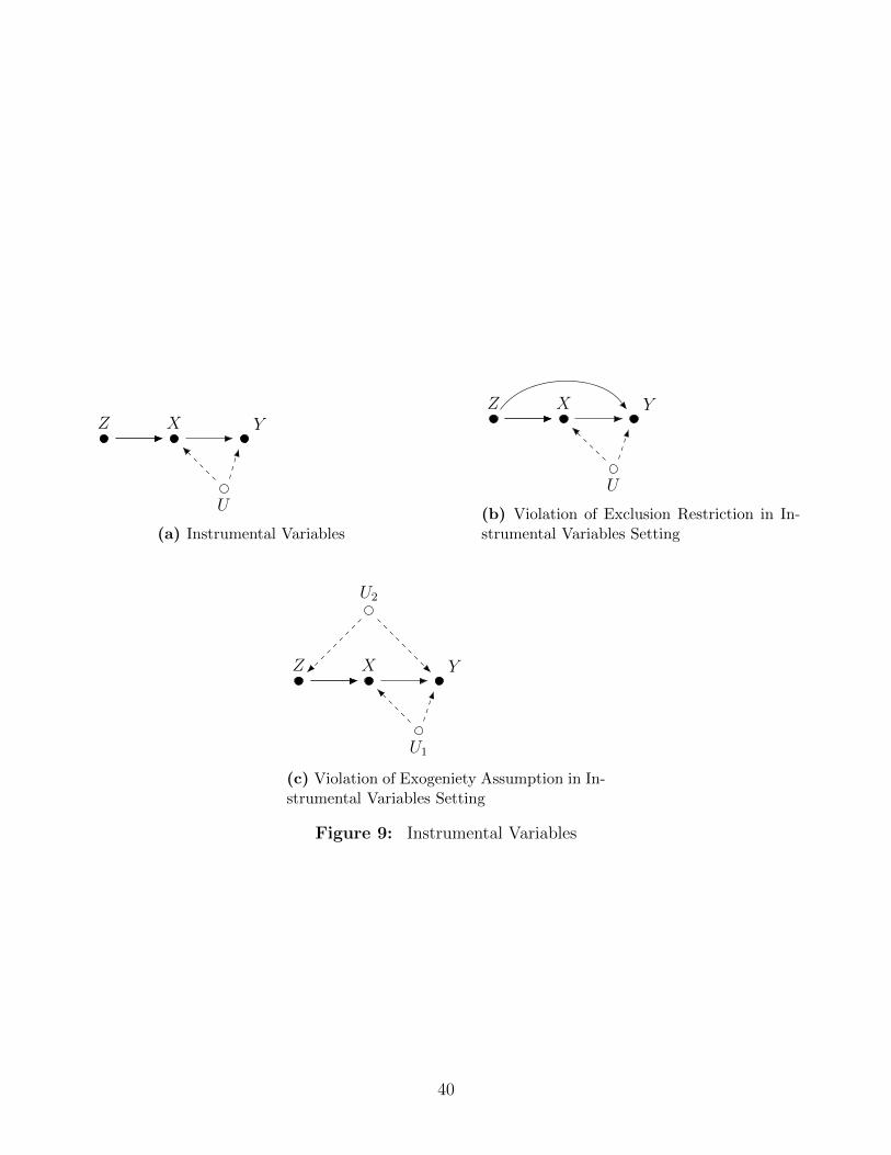
Z X Y
U
(a) Instrumental Variables
Z X Y
U
(b) Violation of Exclusion Restriction in In-strumental Variables Setting
Z X Y
U1
U2
(c) Violation of Exogeniety Assumption in In-strumental Variables Setting
Figure 9: Instrumental Variables
40
there are no direct effect of the instrument Z on the outcome Y . If such a direct effect were
present the DAG would look like Figure 9(b). The second key assumption is that there is no
unmeasured confounder that affects the instrument and the outcome Y . The DAG in Figure
9(c) has such an unmeasured confounder. In the PO approach in Angrist et al. [1996] the start-
ing point is the postulation of the potential outcomes Yi(z, x), indexed by both the treatment
and the instrument, and the potential treatment status Xi(z), indexed by the instrument. The
first assumption is the exclusion restriction that the potential outcomes do not vary with the
instrument, Yi(z, x) = Yi(z′, x) for all z, z′, and the second is an unconfoundedness assumption,
Zi ⊥⊥ (Yi(0, 0), Yi(0, 1), Yi(1, 0), Yi(1, 1), Xi(0), Xi(1)). Again one may well find the graphical
representation of these assumptions more attractive or accessible than the algebraic representa-
tion in the PO framework, or the other way around.
A third key assumption in the instrumental variables setting is the monotonicity condition
that the instrument has a monotone effect on the treatment. In the PO formulation the as-
sumption is Xi(1) ≥ Xi(0), also referred to as the no-defiance assumption (Imbens and Angrist
[1994], Baker and Lindeman [1994], Angrist et al. [1996], Baker et al. [2016]). This assumption
captures the notion that the instrument is an incentive. Although agents need not respond
to such incentives (Xi(1) may be equal to Xi(0) for some individuals), they do not respond
perversely to them (there are no individuals with Xi(1) < Xi(0), the so-called defiers). In
economics much information comes in the form of such monotonicity, or more generally, shape
restrictions. Utility functions are typically at least weakly increasing in their arguments (e.g.,
quantities of goods, leisure) over the relevant ranges, as well as concave. Combined with budget
constraints this leads to demand functions being decreasing in prices. By the same argument,
instruments that can be interpreted as changing incentives lead to responses that are monotone
in these instruments. Because the compliance types are defined explicitly in terms of potential
outcomes, this condition is easy to articular in the PO framework. DAGs do not naturally
represent such conditions, as was pointed out in [Imbens and Rubin, 1995] in a comment on
[Pearl, 1995]. Twenty-five years later this has not been addressed, although that may change:
“Judging from my discussions with @eliasbareinboim and @analisereal, I think that
incorporating shape restrictions such as monotonicity into the [DAG] framework, to
see how it creates opportunities for identification, will be high on the agenda of com-
puter scientists in the coming years.” (April 4th, 2019, Twitter, Paul Hunermund,
41
@PHuenermund)
There are already some attemps to include these assumptions in the DAGs, e.g., [Steiner, Kim,
Hall, and Su, 2017], but I do not find these DAGs particularly illuminating.
Given the assumptions, the identification results are also easier to derive in the PO frame-
work. The early results in the instrumental variables literature with heterogenous treatment
effects established that the average effect of the treatment was not identified in general (Heck-
man [1990]). In addition bounds were derived ([Robins, 1986, Manski, 1990, Balke and Pearl,
1997, Swanson, Hernan, Miller, Robins, and Richardson, 2018]. Such results follow easily in both
the DAG and PO approaches. However, the subsequent identification result for the average effect
for compliers, the Local Average Treatment Effect (LATE),
τ late = E[Yi(1)− Yi(0)|Xi(0) = 0, Xi(1) = 1],
is more difficult to derive using a graphical approach. In fact, setting the problem up in the
PO framework led ([Imbens and Angrist, 1994, Angrist et al., 1996]) to their result. The PO
framework is a natural one here because the very definition of the LATE estimand involves
the potential outcomes Xi(0) and Xi(1) that define compliance status. In passing TBOW
acknowledges the difficulty the DAG approach has in this setting:
“To sum up, instrumental variables are an important tool in that they help us
uncover causal information that goes beyond the do-calculus. [...] if we can justify an
assumption like monotonicity ... on scientific grounds, then a more special-purpose
tool like instrumental variables is worth considering.” (TBOW, p.257)
This reflects more general difficulties in the DAG framework to capture individual level hetero-
geneity ([Hartman, Grieve, Ramsahai, and Sekhon, 2015, Wager and Athey, 2017]).
TBOW also discusses instrumental variables in the context of one of the classic examples,
non-compliance in a randomized experiment (e.g., Imbens and Rubin [1997]). Here the instru-
ment is the random assignment to either the cholesterol drug or a placebo. The treatment
of interest or endogenous variable is the receipt of the cholesterol drug. The outcome is the
subsequent cholesterol level. In this case the instrument is unconfounded by design: the ran-
domization rules out the presence of the unmeasured confounders in Figure 9(c). However, the
exclusion restriction that rules out the direct effect in Figure 9(b) is still controversial. Although
42

x
y
c
E(y|x)
(a) Conditional Expectation
x
f(x)
c
(b) Density
Figure 10: Regression Discontinuity
TBOW blithly dismisses concerns with the exclusion restriction in this setting by writing that
“Common sense suggests that there is no way that receiving a particular random number (Z)
would affect cholesterol (Y )” (TBOW, p. 253), there may in fact well be violations of the
exclusion restriction. For example, side-effects of the actual drug could lead the patients to non-
comply, but seek other treatments. Simply leaving out an arrow because of “common sense”
may not be sufficient to make identifying assumptions. The careful discussion of such possible
violations of the exclusion restriction from a PO perspective is a hallmark of modern empirical
economic practice, through sensitivity analyses (e.g., Angrist et al. [1996]) and other supple-
mentary analyses (Athey and Imbens [2017], Ding et al. [2017]). For example, in the seminal
Angrist [1990] instrumenal variables application it is helpful to consider separately the exclusion
restriction (the absence of a direct effect of the instrument, the draft lottery number, on the
outcome, earnings) for never-takers and always-takers, because it may be much more plausible
for some groups than for others. Such discussions underline how rare it is in practice to have
settings where the absence of arrows is immediately credible.
A closely related setting where DAGs have also not added much insight is in regression
discontinuity designs (RDDs) (Thistlewaite and Campbell [1960], Imbens and Lemieux [2008],
Calonico et al. [2014], Lee and Lemieux [2010]). In the sharp RDD the assignment rule for the
binary treatment X is a deterministic function of a running pretreatment variable W :
X(w) = 1w≤c,
for some fixed threshold c. The average causal effect of the treatment at the threshold is
identified in that case under smoothness conditions on the expected values or the distribution
of the potential outcomes conditional on the running variable. A long time after RD designs
43
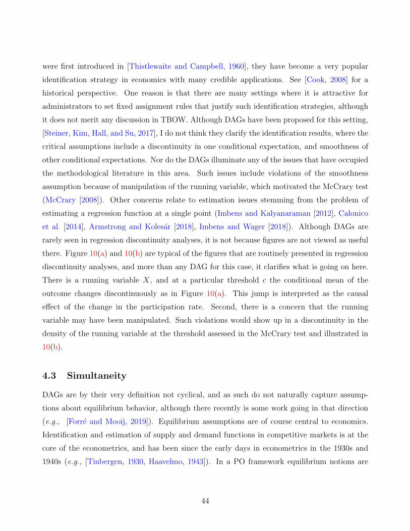
were first introduced in [Thistlewaite and Campbell, 1960], they have become a very popular
identification strategy in economics with many credible applications. See [Cook, 2008] for a
historical perspective. One reason is that there are many settings where it is attractive for
administrators to set fixed assignment rules that justify such identification strategies, although
it does not merit any discussion in TBOW. Although DAGs have been proposed for this setting,
[Steiner, Kim, Hall, and Su, 2017], I do not think they clarify the identification results, where the
critical assumptions include a discontinuity in one conditional expectation, and smoothness of
other conditional expectations. Nor do the DAGs illuminate any of the issues that have occupied
the methodological literature in this area. Such issues include violations of the smoothness
assumption because of manipulation of the running variable, which motivated the McCrary test
(McCrary [2008]). Other concerns relate to estimation issues stemming from the problem of
estimating a regression function at a single point (Imbens and Kalyanaraman [2012], Calonico
et al. [2014], Armstrong and Kolesar [2018], Imbens and Wager [2018]). Although DAGs are
rarely seen in regression discontinuity analyses, it is not because figures are not viewed as useful
there. Figure 10(a) and 10(b) are typical of the figures that are routinely presented in regression
discontinuity analyses, and more than any DAG for this case, it clarifies what is going on here.
There is a running variable X, and at a particular threshold c the conditional mean of the
outcome changes discontinuously as in Figure 10(a). This jump is interpreted as the causal
effect of the change in the participation rate. Second, there is a concern that the running
variable may have been manipulated. Such violations would show up in a discontinuity in the
density of the running variable at the threshold assessed in the McCrary test and illustrated in
10(b).
4.3 Simultaneity
DAGs are by their very definition not cyclical, and as such do not naturally capture assump-
tions about equilibrium behavior, although there recently is some work going in that direction
(e.g., [Forre and Mooij, 2019]). Equilibrium assumptions are of course central to economics.
Identification and estimation of supply and demand functions in competitive markets is at the
core of the econometrics, and has been since the early days in econometrics in the 1930s and
1940s (e.g., [Tinbergen, 1930, Haavelmo, 1943]). In a PO framework equilibrium notions are
44
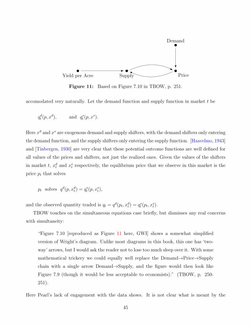
Yield per Acre Supply Price
Demand
Figure 11: Based on Figure 7.10 in TBOW, p. 251.
accomodated very naturally. Let the demand function and supply function in market t be
qdt (p, xd), and qst (p, xs).
Here xd and xs are exogenous demand and supply shifters, with the demand shifters only entering
the demand function, and the supply shifters only entering the supply function. [Haavelmo, 1943]
and [Tinbergen, 1930] are very clear that these potential outcome functions are well defined for
all values of the prices and shifters, not just the realized ones. Given the values of the shifters
in market t, xdt and xst respectively, the equilibrium price that we observe in this market is the
price pt that solves
pt solves qd(p, xdt ) = qst (p, xst),
and the observed quantity traded is qt = qd(pt, xdt ) = qst (pt, x
st).
TBOW touches on the simultaneous equations case briefly, but dismisses any real concerns
with simultaneity:
“Figure 7.10 [reproduced as Figure 11 here, GWI] shows a somewhat simplified
version of Wright’s diagram. Unlike most diagrams in this book, this one has ‘two-
way’ arrows, but I would ask the reader not to lose too much sleep over it. With some
mathematical trickery we could equally well replace the Demand→Price→Supply
chain with a single arrow Demand→Supply, and the figure would then look like
Figure 7.9 (though it would be less acceptable to economists).” (TBOW, p. 250-
251).
Here Pearl’s lack of engagement with the data shows. It is not clear what is meant by the
45
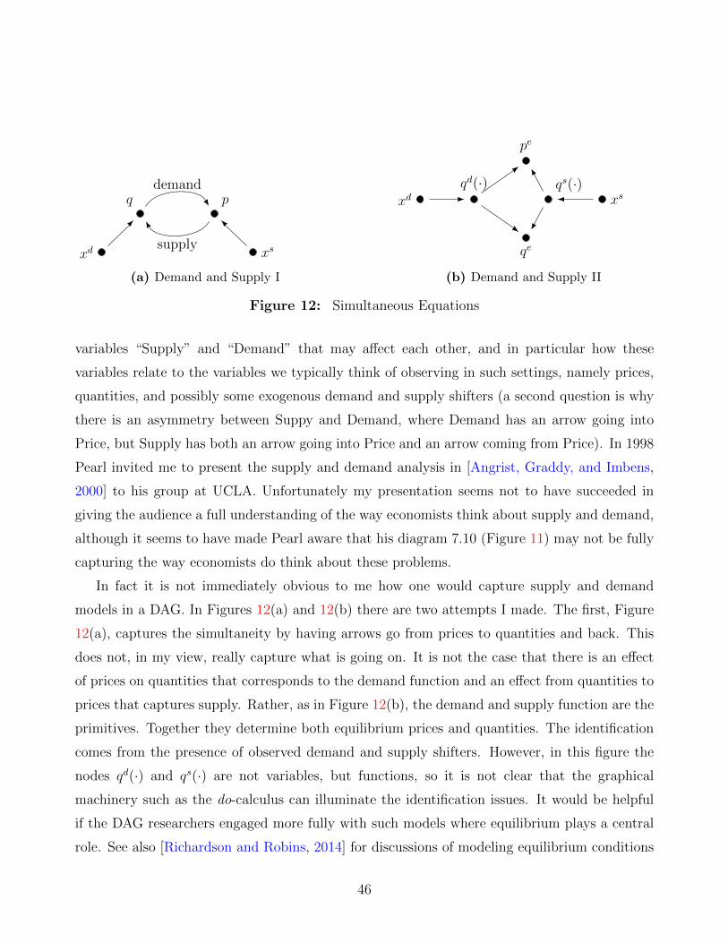
xd
q p
xs
demand
supply
(a) Demand and Supply I
xdqd(·) qs(·)
xs
pe
qe
(b) Demand and Supply II
Figure 12: Simultaneous Equations
variables “Supply” and “Demand” that may affect each other, and in particular how these
variables relate to the variables we typically think of observing in such settings, namely prices,
quantities, and possibly some exogenous demand and supply shifters (a second question is why
there is an asymmetry between Suppy and Demand, where Demand has an arrow going into
Price, but Supply has both an arrow going into Price and an arrow coming from Price). In 1998
Pearl invited me to present the supply and demand analysis in [Angrist, Graddy, and Imbens,
2000] to his group at UCLA. Unfortunately my presentation seems not to have succeeded in
giving the audience a full understanding of the way economists think about supply and demand,
although it seems to have made Pearl aware that his diagram 7.10 (Figure 11) may not be fully
capturing the way economists do think about these problems.
In fact it is not immediately obvious to me how one would capture supply and demand
models in a DAG. In Figures 12(a) and 12(b) there are two attempts I made. The first, Figure
12(a), captures the simultaneity by having arrows go from prices to quantities and back. This
does not, in my view, really capture what is going on. It is not the case that there is an effect
of prices on quantities that corresponds to the demand function and an effect from quantities to
prices that captures supply. Rather, as in Figure 12(b), the demand and supply function are the
primitives. Together they determine both equilibrium prices and quantities. The identification
comes from the presence of observed demand and supply shifters. However, in this figure the
nodes qd(·) and qs(·) are not variables, but functions, so it is not clear that the graphical
machinery such as the do-calculus can illuminate the identification issues. It would be helpful
if the DAG researchers engaged more fully with such models where equilibrium plays a central
role. See also [Richardson and Robins, 2014] for discussions of modeling equilibrium conditions
46
from a non-economic perspective.
4.4 Unconfoundedness, The Choice of Conditioning Variables and
M-Bias
The unconfoundedness setting where the researcher adjusts for some variables in order to esti-
mate the causal effect of a binary treatment on some outcome is probably the most important
one in practice in the modern CI literature. There is much theoretical statistical theory devel-
oped for this case and it underlies much empirical work in economics. In the PO literature the
starting point is the assumption that conditional on the observed confounders Wi the cause Xi
is independent of the potential outcomes Yi(0) and Yi(1), or in the standard notation,
Xi ⊥⊥(Yi(0), Yi(1)
) ∣∣∣ Wi. (4.1)
A classic example is the Lalonde study (LaLonde [1986]), which has been re-analyzed many
times (e.g., Heckman and Hotz [1989], Dehejia and Wahba [1999], Abadie and Imbens [2011]),
and which currently is a standard data set on which to try out new methods (see [Athey et al.,
2019a] for a discussion regarding simulation studies in this context). In this study the treatment
of interest is a labor market training program, the outcome is earnings, and the eight pre-
treatment variables include measures of educational achievement, ethnicity, marital status, age,
and prior measures of annual earnings. One DAG corresponding to this is Figure 8(a). We
could also include any number of arrows between the pre-treatment variable without changing
the identification strategy based on adjusting for the full set of pre-treatment variables.
One may wish to argue whether the DAG here expresses the content of the critical assumption
more clearly than the conditional independence statement in (4.1). [Pearl, 2012] takes a strong
view on this:
“The weakness of this [the potential outcome, GWI] approach surfaces in the prob-
lem formulation phase where, deprived of diagrams and structural equations, re-
searchers are forced to express the (inescapable) assumption set A in a language
totally removed from scientific knowledge, for example, in the form of conditional
independencies among counterfactual variables” ([Pearl, 2012] p. 16-17).
47
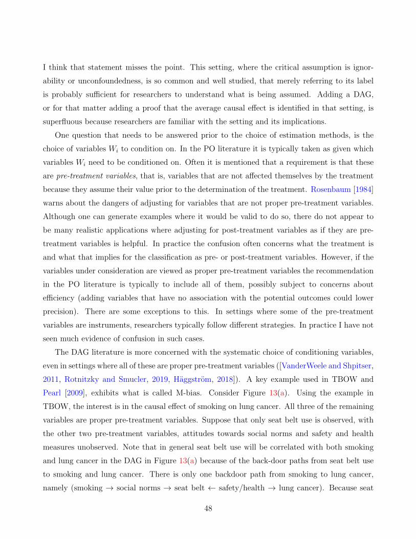
I think that statement misses the point. This setting, where the critical assumption is ignor-
ability or unconfoundedness, is so common and well studied, that merely referring to its label
is probably sufficient for researchers to understand what is being assumed. Adding a DAG,
or for that matter adding a proof that the average causal effect is identified in that setting, is
superfluous because researchers are familiar with the setting and its implications.
One question that needs to be answered prior to the choice of estimation methods, is the
choice of variables Wi to condition on. In the PO literature it is typically taken as given which
variables Wi need to be conditioned on. Often it is mentioned that a requirement is that these
are pre-treatment variables, that is, variables that are not affected themselves by the treatment
because they assume their value prior to the determination of the treatment. Rosenbaum [1984]
warns about the dangers of adjusting for variables that are not proper pre-treatment variables.
Although one can generate examples where it would be valid to do so, there do not appear to
be many realistic applications where adjusting for post-treatment variables as if they are pre-
treatment variables is helpful. In practice the confusion often concerns what the treatment is
and what that implies for the classification as pre- or post-treatment variables. However, if the
variables under consideration are viewed as proper pre-treatment variables the recommendation
in the PO literature is typically to include all of them, possibly subject to concerns about
efficiency (adding variables that have no association with the potential outcomes could lower
precision). There are some exceptions to this. In settings where some of the pre-treatment
variables are instruments, researchers typically follow different strategies. In practice I have not
seen much evidence of confusion in such cases.
The DAG literature is more concerned with the systematic choice of conditioning variables,
even in settings where all of these are proper pre-treatment variables ([VanderWeele and Shpitser,
2011, Rotnitzky and Smucler, 2019, Haggstrom, 2018]). A key example used in TBOW and
Pearl [2009], exhibits what is called M-bias. Consider Figure 13(a). Using the example in
TBOW, the interest is in the causal effect of smoking on lung cancer. All three of the remaining
variables are proper pre-treatment variables. Suppose that only seat belt use is observed, with
the other two pre-treatment variables, attitudes towards social norms and safety and health
measures unobserved. Note that in general seat belt use will be correlated with both smoking
and lung cancer in the DAG in Figure 13(a) because of the back-door paths from seat belt use
to smoking and lung cancer. There is only one backdoor path from smoking to lung cancer,
namely (smoking → social norms → seat belt ← safety/health → lung cancer). Because seat
48
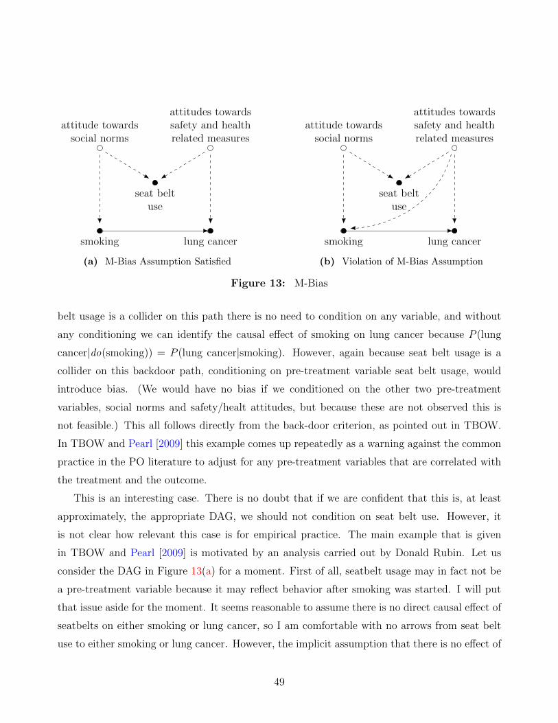
attitude towardssocial norms
smoking
seat beltuse
attitudes towardssafety and healthrelated measures
lung cancer
(a) M-Bias Assumption Satisfied
attitude towardssocial norms
smoking
seat beltuse
attitudes towardssafety and healthrelated measures
lung cancer
(b) Violation of M-Bias Assumption
Figure 13: M-Bias
belt usage is a collider on this path there is no need to condition on any variable, and without
any conditioning we can identify the causal effect of smoking on lung cancer because P (lung
cancer|do(smoking)) = P (lung cancer|smoking). However, again because seat belt usage is a
collider on this backdoor path, conditioning on pre-treatment variable seat belt usage, would
introduce bias. (We would have no bias if we conditioned on the other two pre-treatment
variables, social norms and safety/healt attitudes, but because these are not observed this is
not feasible.) This all follows directly from the back-door criterion, as pointed out in TBOW.
In TBOW and Pearl [2009] this example comes up repeatedly as a warning against the common
practice in the PO literature to adjust for any pre-treatment variables that are correlated with
the treatment and the outcome.
This is an interesting case. There is no doubt that if we are confident that this is, at least
approximately, the appropriate DAG, we should not condition on seat belt use. However, it
is not clear how relevant this case is for empirical practice. The main example that is given
in TBOW and Pearl [2009] is motivated by an analysis carried out by Donald Rubin. Let us
consider the DAG in Figure 13(a) for a moment. First of all, seatbelt usage may in fact not be
a pre-treatment variable because it may reflect behavior after smoking was started. I will put
that issue aside for the moment. It seems reasonable to assume there is no direct causal effect of
seatbelts on either smoking or lung cancer, so I am comfortable with no arrows from seat belt
use to either smoking or lung cancer. However, the implicit assumption that there is no effect of
49

attitudes towards safety and health-related measures on smoking seems very implausible. In all
the discussions of this example, Pearl never discusses whether this assumption is plausible. In
order to use these methods, one needs to carefully consider every absent link, and in a setting
with as many variables as there are in Figure 13(b) that is a daunting task. Now suppose we
allow for one such direct effect, leading to the DAG in Figure 13(b), or alternatively with an
arrow from attitudes towards social norms to cancer. Now the causal effect of smoking on lung
cancer is not identified. Conditioning on seat belt use introduces a new bias, but not adjusting
for differences in seat belt use between smokers and non-smokers leaves a bias. What to do?
Here seat belt use is essentially a proxy for the unobserved attitude variable, and whether to
use it is a difficult question that does not have a single right anwer. The researcher has to make
a choice which of the two evils is the lesser one, or possibly do a sensivity analysis. I am not
sure whether adjusting for seat belt usage between smokers and non-smokers, as Rubin did, is
a good thing or not, but certainly I would not rule out doing this. The recent analysis in [Ding
and Miratrix, 2015] suggests that, both in this specific example, and more generally when there
is concern with confounding as well as M-bias, adjusting may still be superior. Beyond that, I
want to point out that that, as in the front-door criterion setting, even in the examples TBOW
chooses to discuss, it is not at all clear that the method that TBOW favors actually works. This
is particularly important because TBOW introduces this example after admitting that there
was concern that such a DAG might be very implausible:
“When I started showing this diagram to statisticians in the 1990s, some of them
laughed it off and said that such a diagram was extremely unlikely to occur in
practice. I disagree!” (TBOW, p. 161)
Another way to make the point that this may be an unusual setting in practice, note that if
the DAG in Figure 13(a) is correct, it means that we can identify the causal effect of smoking
on lung cancer, but we cannot identify the effect for those who wear seat belts, because there
is a hidden confounder there, nor can we identify the effect for those not wearing seat belts,
because there is a hidden confounder there. Mixing those who wear seat belts and those who do
not, exactly cancels the two biases and leaves us with a valid casusal effect. This does appear
an “extremely unlikely” setting.
To conclude this discussion, let us return to the Lalonde study. The M-bias argument would
suggest that if we carefully model the causal relationships between all eight of the pre-treatment
50
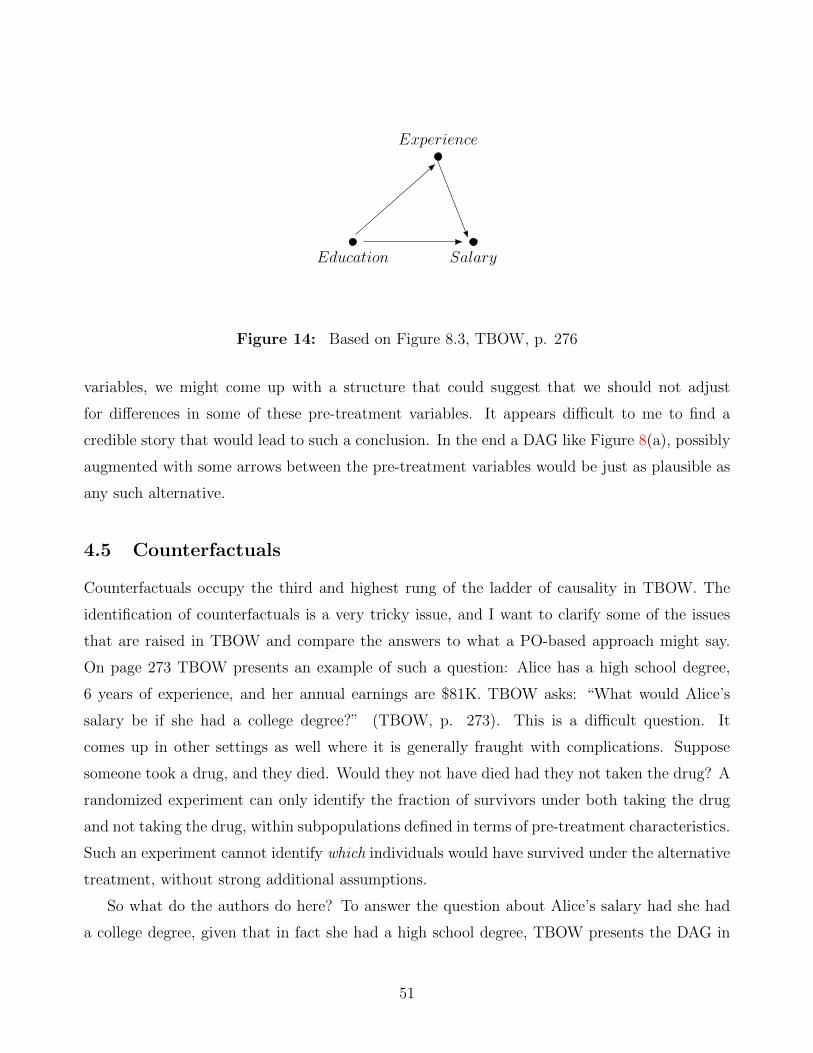
Education Salary
Experience
Figure 14: Based on Figure 8.3, TBOW, p. 276
variables, we might come up with a structure that could suggest that we should not adjust
for differences in some of these pre-treatment variables. It appears difficult to me to find a
credible story that would lead to such a conclusion. In the end a DAG like Figure 8(a), possibly
augmented with some arrows between the pre-treatment variables would be just as plausible as
any such alternative.
4.5 Counterfactuals
Counterfactuals occupy the third and highest rung of the ladder of causality in TBOW. The
identification of counterfactuals is a very tricky issue, and I want to clarify some of the issues
that are raised in TBOW and compare the answers to what a PO-based approach might say.
On page 273 TBOW presents an example of such a question: Alice has a high school degree,
6 years of experience, and her annual earnings are $81K. TBOW asks: “What would Alice’s
salary be if she had a college degree?” (TBOW, p. 273). This is a difficult question. It
comes up in other settings as well where it is generally fraught with complications. Suppose
someone took a drug, and they died. Would they not have died had they not taken the drug? A
randomized experiment can only identify the fraction of survivors under both taking the drug
and not taking the drug, within subpopulations defined in terms of pre-treatment characteristics.
Such an experiment cannot identify which individuals would have survived under the alternative
treatment, without strong additional assumptions.
So what do the authors do here? To answer the question about Alice’s salary had she had
a college degree, given that in fact she had a high school degree, TBOW presents the DAG in
51

Figure 14. The authors then go further, and set up a Structural Causal Model, where they specify
salary (Y ) as a function of education (X) and experience (W ) and an unobserved component,
and similarly for experience as a function of education and an unobserved component as
Y = fY (X,W,UY ), and W = fW (X,UW ).
They then simplify things “assuming linear functions throughout” (TBOW, p. 277):
Y = α0 + α1X + α2W + UY , W = β0 + β1X + UW .
This allows them to first estimate the coefficients (α0, α1, β0, β1, β2) and then, importantly, the
unobserved components UY and UW for Alice as
UY,Alice = YAlice − α0 − α1XAlice − α2WAlice,
UW,Alice = XAlice − β0 − β1XAlice.
Given these coefficients and residuals TBOW then estimates Alice’s salary given a college degree
(Xcollege) as
YAlice = α0 + α1Xcollege + α2
(β0 + β1Xcollege + UW,Alice
)+ UY,Alice.
From a PO perspective a major question concerns the way the residuals UY,Alice and UW,Alice
are used. Starting with potential outcomes, WAlice(highschool) and WAlice(college), the residuals
would be also be indexed by the treatment:
UW,Alice(highschool) = WAlice(highschool)− β0 − β1highschool,
and
UW,Alice(college) = WAlice(college)− β0 − β1college.
There is often a reluctance to rely on assumptions about the association between the residuals
52
UW,Alice(highschool) and UW,Alice(college) from potential outcomes after conditioning on other
variables, whereas the discussion in TBOW implicitly assumes the two are equal. These issues
involving unit-level heterogeneity come up in many settings, e.g, [Sekhon and Shem-Tov, 2017].
Putting aside for a moment the other variables, and assume we actually have a randomized
experiment. We would not be confident that the rank of YAlice(highschool) in the distribution of
high-school salaries would be the same as the rank of YAlice(college) in the distribution of college
salaries (corresponding in the linear case to equality of the residuals UW,Alice(highschool) and
UW,Alice(college)). There is obviously many reasons why an individual who would be relatively
productive given a college degree (e.g., someone with strong cognitive abilities), would not
necessarily be relatively productive with only a high-school degree. The jobs a person would
end up with given a college degree would be different from the one they would have with a high-
school degree, with value placed on different sets of skills. This type of comparative advantage
argument is common in economics, and it is a critical part of the Roy model of occupational
choice ([Roy, 1951]). TBOWs implicit assumption of a single (scalar) unobserved component
is quite distinct from the assumption of linearity of the conditional expectations that TBOW
bundles it with, but it is crucial to the ability to predict Alice’s salary given a college degree.
This is not to say that this type of assumption is never made in economics. The point
is that when it is done well, such assumptions are typically made very explicitly, with full
recognition of the identifying power it has (e.g., the discussion of the rank correlation assumption
in [Chernozhukov and Hansen, 2005]), rather than just as one component of a set of functional
form assumptions the way TBOW does here. It has also received much attention in the discussion
on identifying distributions of treatment effects, as opposed to differences in the distribution of
potential outcomes (see the discussion in [Manski, 1996, Deaton, 2010, Imbens, 2010]). The
way in which TBOW exploits this assumption without being explicit about it undercuts the
arguments advanced in other parts of the book about the transparency of the DAG-based
assumptions relative to the PO formulation.
A second issue is that TBOW is unhappy with the formulation of the critical assumptions
here in terms of the potential outcomes:
“To determine if ED [education] is ignorable [...] we are supposed to judge whether
employees who would have one potential salary, say S1 = s [that is, Y (highschool) =
s], are just as likely to have one level of education as the employees who would have
53

a different potential salary, say S1 = s′ [that is, Y (highschool) = s′]. If you think
this sounds circular, I can only agree with you! ... It is quite a cognitive nightmare.”
(TBOW, p. 282).
These assumptions may be challenging, but of course the formulation agrees closely with stan-
dard economic theory. Since [Roy, 1951] and [Mincer, 1974] economists model individuals choos-
ing whether to go to college partly by comparing their utility (e.g., earnings) if they were to go
to college with the utility if they were not to go to college, that is, by comparing their potential
outcomes Y (highschool) and Y (college), or expecations thereof. It is precisely the important
role the potential outcomes play in the formulation of the choice models (e.g., the random utility
choice models in [McFadden et al., 1973] and [Manski, 1977]) that makes the PO framework a
natural one in economics that resonates with practitioners.
4.6 An Example: Identifying the Returns to Education
Let me finally discuss an empirical setting where economists have used a variety of identification
strategies for the same substantive problem and compare DAGs and econometric identification
strategies. The focus is on estimating the returns to education, or, more specifically, the effect
of years of education on the logarithm of earnings. Since [Mincer, 1974] economists have focused
on the effect on the logarithm of earnings in order to interpret the effect as a return, similar to
the return on financial investments.
The basic data consists of observations on years of education and the logarithm of earnings.
Figure 15(a) shows the simplest strategy in a DAG format, directly comparing people with
different levels of education. Typically this would be implemented by linear regression of log
earnings on years of education, but in a more flexible approach one could simply compare average
values for log earnings by education levels. The concern is that this is too simple a model,
and that there may be an unmeasured confounder. In substantive discussions the unmeasured
confounder is typically thought of as unmeasured ability, as in Figure 15(b). Omitted variable
bias arguments suggest that failure to adjust for differences in ability would lead to an upward
bias in the estimated returns to education, because it is likely that ability is positively correlated
with levels of education and with the potential outcomes. See [Griliches, 1977, Card, 1999, 2001]
for general discussions.
In response to these concerns econometricians have used a variety of approaches. I will briefly
54
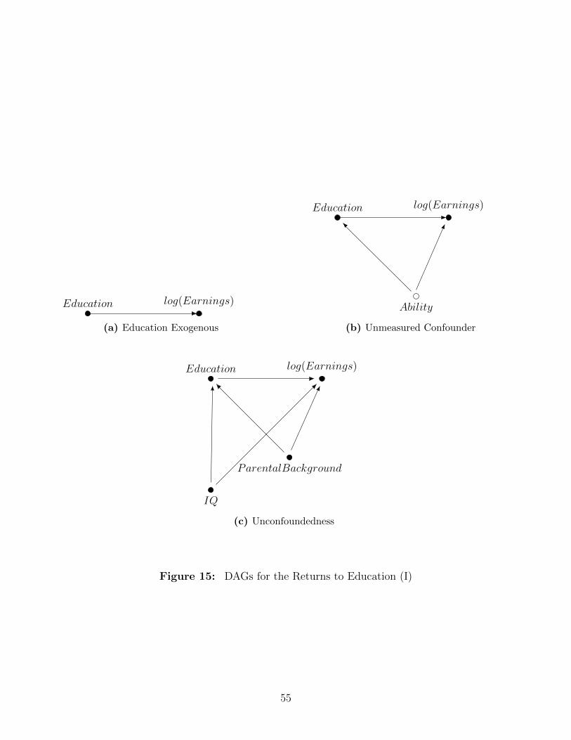
Education log(Earnings)
(a) Education Exogenous
Education log(Earnings)
Ability
(b) Unmeasured Confounder
Education log(Earnings)
ParentalBackground
IQ
(c) Unconfoundedness
Figure 15: DAGs for the Returns to Education (I)
55
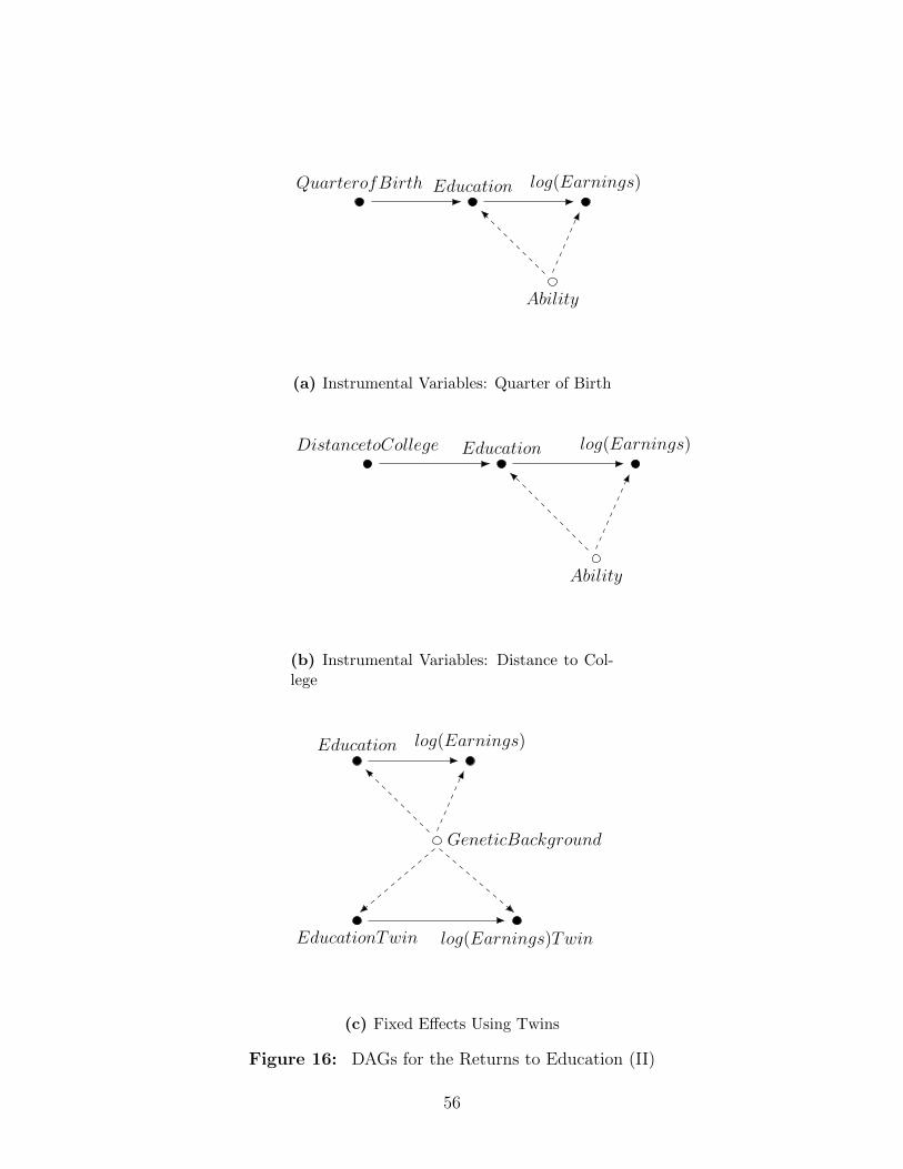
Education log(Earnings)
Ability
QuarterofBirth
(a) Instrumental Variables: Quarter of Birth
Education log(Earnings)
Ability
DistancetoCollege
(b) Instrumental Variables: Distance to Col-lege
Education log(Earnings)
GeneticBackground
EducationTwin log(Earnings)Twin
(c) Fixed Effects Using Twins
Figure 16: DAGs for the Returns to Education (II)
56
discuss some of them and attempt to illustrate them in DAGs. One approach is to attempt to
measure ability. For example, one may use parental background measures, including parental
education or socio-economic status. Researchers have also attempted to directly measure ability,
through test scores or iq tests. Using both parental background and iq scores leads to a DAG as
in Figure 15(c) where adjusting for the pre-treatment variables leads to unbiased estimates of
the effect of interest. Of course there may be concerns that variables like parental background
do not have a direct causal effect on the child’s later earnings, and that this is merely a proxy
for unobserved ability. In practice, however, researchers have attempted to control as much
as possible for variables that are proper pre-treatment (that is, prior to educational decisions
being made), without concerns about introducing M-bias. It is rare to see researchers use post-
treatment variables as controls in this approach.
Another strategy has been to use instrumental variables approaches, based on instruments
that change the incentives to acquire additional formal education. One classic example is the
[Angrist and Krueger, 1991] study using quarter of birth as an instrument, as in Figures 16(a).
A second classic example is [Card, 1993] using distance to college as an instrument, as in 16(b).
Both applications are complicated. Although originally they assumed constant treatment effects,
they are now typically interpreted as weighted average effects for compliers with the weights
varying by education levels [Angrist and Imbens, 1995]. There are also concerns with the
exclusion restriction in both cases. There may also be concerns with the monotonicity condition
in the college distance application if the closest college is a two-year college. The [Angrist and
Krueger, 1991] study also spawned a big literature on weak instrument problems (e.g., [Staiger
and Stock, 1997, Andrews and Stock, 2006, Chamberlain and Imbens, 2004]). These problems
are often naturally discussed in a PO framework, with the benefit of putting this in a DAG
unclear.
Yet another strategy has been to look for siblings, or, going even further, twins, as in [Ashen-
felter and Krueger, 1994, Ashenfelter and Rouse, 1998]. The estimation procedure regresses
differences in the logarithm of earnings on differences in years of education. Implicitly there is a
DAG similar to Figures 16(c), but there is additional structure. The causal effect of education
on log earnings is the same for the two members of a twin pair, and similarly the causal effect
of the unobserved confounder (genetic background) on education and earnings is the same for
both members of the twin. The full set of assumptions here is difficult to capture in a DAG.
There is some connection between this identification strategy and the multiple causes approach
57
in [Wang and Blei, 2018]. They assume that there is an unobserved confounder that affects both
causes. In the twins case this is the genetic background that is common to both members of the
twin pair. The additional structure in the twins case (symmetry between the two members of
the twin pairs) helps pin down the shared confounder, but there may be additional links that
can be exploited. These strategies are not without controversy: it is not always clear that the
variation in education levels between siblings or twins is exogenous (see [Card, 1999, 2001]).
This is a rich literature full of clever attempts to get closer to the causal effect of education.
The challenge for the graphical literature is to come up with novel strategies that shed light on
substantive questions like this.
5 Conclusion
TBOW and the DAG approach fully deserve the attention of all researchers and users of causal
inference as one of its leading methodologies. Is it more than that? Should it be the framework
of choice for all causal questions, everywhere, or at least in the social sciences, as TBOW argues?
Should it be the starting point for teaching about causality? In my view the answer to both
questions is no. The questions it currently answers well are not the ones that are the most
pressing ones in practice. Conversely, for the most common and important questions the PO
framework is in my view an attractive one in social sciences, and one that resonates well with
economic theory by effectively incorporating restrictions beyond conditional independencies.
Moreover, for the problems where DAGs could contribute substantially, the most important
issue holding back the DAGs is the lack of convincing empirical applications. History suggests
that credible applications are what drives the adoption of new methodologies in economics and
other social sciences, not mathematical elegance or rhetoric. It is studies such as [LaLonde,
1986], [Card, 1990], [Angrist, 1990], [Angrist and Krueger, 1991], and [Ashenfelter and Krueger,
1994] that spurred the credibility revolution and the adoption of the PO framework, not the
theoretical advances – they came later. There have not been similar applications of the DAG
framework, and more papers discussing toy models will not be sufficient to convince economists
to use this framework.
58
References
Alberto Abadie and Matias D Cattaneo. Econometric methods for program evaluation. Annual
Review of Economics, 10:465–503, 2018.
Alberto Abadie and Javier Gardeazabal. The economic costs of conflict: A case study of the
basque country. American Economic Review, 93(-):113–132, 2003.
Alberto Abadie and Guido W Imbens. Bias-corrected matching estimators for average treatment
effects. Journal of Business & Economic Statistics, 29(1):1–11, 2011.
Alberto Abadie, Alexis Diamond, and Jens Hainmueller. Synthetic control methods for com-
parative case studies: Estimating the effect of california’s tobacco control program. Journal
of the American statistical Association, 105(490):493–505, 2010.
Donald Andrews and James H. Stock. Inference with weak instruments. 2006.
Isaiah Andrews and Emily Oster. A simple approximation for evaluating external validity bias.
Economics Letters, 178:58–62, 2019.
Isaiah Andrews, Matthew Gentzkow, and Jesse M Shapiro. Measuring the sensitivity of parame-
ter estimates to estimation moments. The Quarterly Journal of Economics, 132(4):1553–1592,
2017.
Joshua Angrist and Alan Krueger. Empirical strategies in labor economics. Handbook of Labor
Economics, 3, 2000.
Joshua D Angrist. Lifetime earnings and the Vietnam era draft lottery: Evidence from social
security administrative records. The American Economic Review, pages 313–336, 1990.
Joshua D Angrist and Guido W Imbens. Two-stage least squares estimation of average causal
effects in models with variable treatment intensity. Journal of the American statistical
Association, 90(430):431–442, 1995.
Joshua D Angrist and Alan Krueger. Does compulsory schooling affect schooling and earnings.
Quarterly Journal of Economics, CVI(4):979–1014, 1991.
59

Joshua D Angrist and Jorn-Steffen Pischke. Mostly harmless econometrics: An empiricist’s
companion. Princeton University Press, 2008.
Joshua D Angrist and Jorn-Steffen Pischke. The credibility revolution in empirical economics:
How better research design is taking the con out of econometrics. Journal of economic
perspectives, 24(2):3–30, 2010.
Joshua D Angrist, Guido W Imbens, and Donald B. Rubin. Identification of causal effects using
instrumental variables. Journal of the American Statistical Association, 91:444–472, 1996.
Joshua D Angrist, Kathryn Graddy, and Guido W Imbens. The interpretation of instrumental
variables estimators in simultaneous equations models with an application to the demand for
fish. The Review of Economic Studies, 67(3):499–527, 2000.
Timothy B Armstrong and Michal Kolesar. Optimal inference in a class of regression models.
Econometrica, 86(2):655–683, 2018.
Peter Aronow. A general method for detecting interference between units in randomized exper-
iments. Sociological Methods & Research, 41(1):3–16, 2012.
Peter M. Aronow and Cyrus Samii. Estimating average causal effects under interference between
units, 2013.
Orley Ashenfelter and Alan Krueger. Estimates of the economic return to schooling from a new
sample of twins. The American Economic Review, 84(5):1157–1173, 1994.
Orley Ashenfelter and Cecilia Rouse. Income, schooling, and ability: Evidence from a new
sample of identical twins. The Quarterly Journal of Economics, 113(1):253–284, 1998.
Susan Athey and Guido Imbens. Recursive partitioning for heterogeneous causal effects.
Proceedings of the National Academy of Sciences, 113(27):7353–7360, 2016.
Susan Athey and Guido Imbens. Machine learning methods economists should know about.
manuscript, 2018.
Susan Athey and Guido W Imbens. The state of applied econometrics: Causality and policy
evaluation. Journal of Economic Perspectives, 31(2):3–32, 2017.
60
Susan Athey and Scott Stern. An empirical framework for testing theories about complimentarity
in organizational design. Technical report, National Bureau of Economic Research, 1998.
Susan Athey and Stefan Wager. Efficient policy learning. arXiv preprint arXiv:1702.02896,
2017.
Susan Athey, Raj Chetty, Guido Imbens, and Hyunseung Kang. Estimating treatment effects
using multiple surrogates: The role of the surrogate score and the surrogate index. arXiv
preprint arXiv:1603.09326, 2016.
Susan Athey, Dean Eckles, and Guido W Imbens. Exact p-values for network interference.
Journal of the American Statistical Association, 113(521):230–240, 2018a.
Susan Athey, Guido W Imbens, and Stefan Wager. Approximate residual balancing: debiased
inference of average treatment effects in high dimensions. Journal of the Royal Statistical
Society: Series B (Statistical Methodology), 80(4):597–623, 2018b.
Susan Athey, Guido W Imbens, Jonas Metzger, and Evan M Munro. Using wasserstein generative
adversarial networks for the design of monte carlo simulations. Technical report, National
Bureau of Economic Research, 2019a.
Susan Athey, Julie Tibshirani, Stefan Wager, et al. Generalized random forests. The Annals of
Statistics, 47(2):1148–1178, 2019b.
Stuart G Baker and Karen S Lindeman. The paired availability design: a proposal for evaluating
epidural analgesia during labor. Statistics in Medicine, 13(21):2269–2278, 1994.
Stuart G Baker, Barnett S Kramer, and Karen S Lindeman. Latent class instrumental variables:
a clinical and biostatistical perspective. Statistics in medicine, 35(1):147–160, 2016.
Alexander Balke and Judea Pearl. Bounds on treatment effects from studies with imperfect
compliance. Journal of the American Statistical Association, 92(439):1171–1176, 1997.
Abhijit V Banerjee and Esther Duflo. The experimental approach to development economics.
Technical report, National Bureau of Economic Research, 2008.
GW Basse, A Feller, and P Toulis. Randomization tests of causal effects under interference.
Biometrika, 2019.
61
Alexandre Belloni, Victor Chernozhukov, Ivan Fernandez-Val, and Chris Hansen. Program
evaluation with high-dimensional data. arXiv preprint arXiv:1311.2645, 2013.
Marianne Bertrand and Sendhil Mullainathan. Are emily and greg more employable than lakisha
and jamal? a field experiment on labor market discrimination. American economic review,
94(4):991–1013, 2004.
Sandra E Black. Do better schools matter? parental valuation of elementary education. The
Quarterly Journal of Economics, 114(2):577–599, 1999.
Peter Buhlmann. Invariance, causality and robustness. arXiv preprint arXiv:1812.08233, 2018.
S. Calonico, Matias Cattaneo, and Rocio Titiunik. Robust nonparametric confidence intervals
for regression-discontinuity designs. Econometrica, 82(6):2295–2326, 2014.
David Card. The impact of the mariel boatlift on the miami labor market. Industrial and Labor
Relation, 43(2):245–257, 1990.
David Card. Using geographic variation in college proximity to estimate the return to schooling.
Technical report, National Bureau of Economic Research, 1993.
David Card. The causal effect of education on earnings. In Handbook of labor economics,
volume 3, pages 1801–1863. Elsevier, 1999.
David Card. Estimating the return to schooling: Progress on some persistent econometric
problems. Econometrica, 69(5):1127–1160, 2001.
Karim Chalak and Halbert White. An extended class of instrumental variables for the estimation
of causal effects. Canadian Journal of Economics/Revue canadienne d’economique, 44(1):1–
51, 2011.
Gary Chamberlain. The general equivalence of granger and sims causality. Econometrica:
Journal of the Econometric Society, pages 569–581, 1982.
Gary Chamberlain and Guido Imbens. Random effects estimators with many instrumental
variables. Econometrica, 72(1):295–306, 2004.
62
Xi Chen, Victor Chernozhukov, Ivan Fernandez-Val, Scott Kostyshak, and Ye Luo. Shape-
enforcing operators for point and interval estimators. arXiv preprint arXiv:1809.01038, 2018.
Victor Chernozhukov and Christian Hansen. An iv model of quantile treatment effects.
Econometrica, 73(1):245–261, 2005.
Victor Chernozhukov, Denis Chetverikov, Mert Demirer, Esther Duflo, Christian Hansen, and
Whitney Newey. Double/debiased/neyman machine learning of treatment effects. American
Economic Review, 107(5):261–65, 2017.
Denis Chetverikov, Andres Santos, and Azeem M Shaikh. The econometrics of shape restrictions.
Annual Review of Economics, 10:31–63, 2018.
Thomas Cook. Waiting for life to arrive: A history of the regression-discontinuity design in
psychology, statistics and economics. Journal of Econometrics, 142(2):636–654, 2008.
David R Cox. Causality: some statistical aspects. Journal of the Royal Statistical Society:
Series A (Statistics in Society), 155(2):291–301, 1992.
David R Cox and Nanny Wermuth. Discussion-causal diagrams for empirical research.
Biometrika, 82(4):688–689, 1995.
Richard K Crump, V Joseph Hotz, Guido W Imbens, and Oscar A Mitnik. Dealing with limited
overlap in estimation of average treatment effects. Biometrika, pages 187–199, 2009.
Scott Cunningham. Causal Inference: The Mixtape. Manuscript, 2018.
Alexander D’Amour, Peng Ding, Avi Feller, Lihua Lei, and Jasjeet Sekhon. Overlap in obser-
vational studies with high-dimensional covariates. arXiv preprint arXiv:1711.02582, 2017.
Sonya Das and Andrew W Lo. Re-inventing drug development: A case study of the i-spy 2
breast cancer clinical trials program. Contemporary clinical trials, 62:168–174, 2017.
Angus Deaton. Instruments, randomization, and learning about development. Journal of
Economic Literature, 48(2):424–455, 2010.
Angus Deaton and Nancy Cartwright. Understanding and misunderstanding randomized con-
trolled trials. Social Science & Medicine, 210:2–21, 2018.
63

Rajeev H Dehejia and Sadek Wahba. Causal effects in nonexperimental studies: Reevaluating
the evaluation of training programs. Journal of the American statistical Association, 94(448):
1053–1062, 1999.
Xavier D’Haultfœuille and Philippe Fevrier. Identification of nonseparable triangular models
with discrete instruments. Econometrica, 83(3):1199–1210, 2015.
Maria Dimakopoulou, Susan Athey, and Guido Imbens. Estimation considerations in contextual
bandits. arXiv preprint arXiv:1711.07077, 2017.
Maria Dimakopoulou, Zhengyuan Zhou, Susan Athey, and Guido Imbens. Balanced linear
contextual bandits. arXiv preprint arXiv:1812.06227, 2018.
Peng Ding and Luke W Miratrix. To adjust or not to adjust? sensitivity analysis of m-bias and
butterfly-bias. Journal of Causal Inference, 3(1):41–57, 2015.
Peng Ding, TJ VanderWeele, and JM Robins. Instrumental variables as bias amplifiers with
general outcome and confounding. Biometrika, 104(2):291–302, 2017.
Julien Dubois, Hiroyuki Oya, J Michael Tyszka, Matthew Howard III, Frederick Eberhardt, and
Ralph Adolphs. Causal mapping of emotion networks in the human brain: framework and
initial findings. Neuropsychologia, 2017.
Patrick Forre and Joris M Mooij. Causal calculus in the presence of cycles, latent confounders
and selection bias. arXiv preprint arXiv:1901.00433, 2019.
Constantine E Frangakis and Donald B Rubin. Principal stratification in causal inference.
Biometrics, 58(1):21–29, 2002.
David A Freedman. Statistical models for causation: what inferential leverage do they provide?
Evaluation review, 30(6):691–713, 2006.
Andrew Gelman. Causality and statistical learning. American Journal of Sociology, 117(3):
955–966, 2011.
Andrew Gelman and Guido Imbens. Why ask why? forward causal inference and reverse causal
questions. Technical report, National Bureau of Economic Research, 2013.
64
Clark Glymour, Richard Scheines, and Peter Spirtes. Discovering causal structure: Artificial
intelligence, philosophy of science, and statistical modeling. Academic Press, 2014.
Adam N Glynn and Konstantin Kashin. Front-door versus back-door adjustment with unmea-
sured confounding: Bias formulas for front-door and hybrid adjustments with application to
a job training program. Journal of the American Statistical Association, 113(523):1040–1049,
2018.
Arthur Stanley Goldberger. A course in econometrics. Harvard University Press, 1991.
Claudia Goldin and Cecilia Rouse. Orchestrating impartiality: The impact of” blind” auditions
on female musicians. American economic review, 90(4):715–741, 2000.
Bryan S Graham. Methods of identification in social networks. Annu. Rev. Econ., 7(1):465–485,
2015.
Clive Granger. Comment. Journal of the American Statistical Association, 81(396):967–968,
1986. doi: 10.1080/01621459.1986.10478358. URL https://doi.org/10.1080/01621459.
1986.10478358.
Clive WJ Granger. Investigating causal relations by econometric models and cross-spectral
methods. Econometrica: Journal of the Econometric Society, pages 424–438, 1969.
Sander Greenland, Judea Pearl, James M Robins, et al. Causal diagrams for epidemiologic
research. Epidemiology, 10:37–48, 1999.
Zvi Griliches. Estimating the returns to schooling: Some econometric problems. Econometrica:
Journal of the Econometric Society, pages 1–22, 1977.
Somit Gupta, Ronny Kohavi, Diane Tang, Ya Xu, Reid Andersen, Eytan Bakshy, Niall Cardin,
Sumita Chandran, Nanyu Chen, Dominic Coey, et al. Top challenges from the first practical
online controlled experiments summit. ACM SIGKDD Explorations Newsletter, 21(1):20–35,
2019.
Trygve Haavelmo. The statistical implications of a system of simultaneous equations.
Econometrica, 11(1):1–12, 1943.
65
Trygve Haavelmo. The probability approach in econometrics. Econometrica, 12(Supplement):
iii–vi+1–115, 1944.
Jenny Haggstrom. Data-driven confounder selection via markov and bayesian networks.
Biometrics, 74(2):389–398, 2018.
Jinyong Hahn, Petra Todd, and Wilbert Van der Klaauw. Identification and estimation of
treatment effects with a regression-discontinuity design. Econometrica, 69(1):201–209, 2001.
Erin Hartman, Richard Grieve, Roland Ramsahai, and Jasjeet S Sekhon. From sate to patt:
combining experimental with observational studies to estimate population treatment effects.
JR Stat. Soc. Ser. A Stat. Soc.(forthcoming). doi, 10:1111, 2015.
James Heckman. Varieties of selection bias. The American Economic Review, 80(2):313–318,
1990.
James Heckman and Rodrigo Pinto. Causal analysis after haavelmo. Econometric Theory, 31
(1):115–151, 2015.
James J Heckman and V Joseph Hotz. Choosing among alternative nonexperimental methods
for estimating the impact of social programs: The case of manpower training. Journal of the
American statistical Association, 84(408):862–874, 1989.
David F Hendry and Mary S Morgan. The foundations of econometric analysis. Cambridge
University Press, 1997.
Miguel A Hernan, John Hsu, and Brian Healy. Data science is science’s second chance to get
causal inference right: A classification of data science tasks. arXiv preprint arXiv:1804.10846,
2018.
Keisuke Hirano, Guido W Imbens, Donald B Rubin, and Xiao-Hua Zhou. Assessing the effect
of an influenza vaccine in an encouragement design. Biostatistics, 1(1):69–88, 2000.
Paul W Holland. Statistics and causal inference. Journal of the American statistical Association,
81(396):945–960, 1986.
Joel L Horowitz. Applied nonparametric instrumental variables estimation. Econometrica, 79
(2):347–394, 2011.
66
Patrik O Hoyer, Dominik Janzing, Joris M Mooij, Jonas Peters, and Bernhard Scholkopf. Nonlin-
ear causal discovery with additive noise models. In Advances in neural information processing
systems, pages 689–696, 2009.
Michael Hudgens and Elizabeth Halloran. Toward causal inference with interference. Journal
of the American Statistical Association, pages 832–842, 2008.
Paul Hunermund and Elias Bareinboim. Causal inference and data-fusion in econometrics. arXiv
preprint arXiv:1912.09104, 2019.
Guido Imbens. The role of the propensity score in estimating dose–response functions.
Biometrika, 87(0):706–710, 2000.
Guido Imbens. Nonparametric estimation of average treatment effects under exogeneity: A
review. Review of Economics and Statistics, pages 1–29, 2004.
Guido Imbens. Better late than nothing: Some comments on deaton (2009) and heckman and
urzua (2009). Journal of Economic Literature, pages 399–423, 2010.
Guido Imbens. Instrumental variables: An econometrician’s perspective. Statistical Science,
(3):323–358, 2014.
Guido Imbens and Karthik Kalyanaraman. Optimal bandwidth choice for the regression dis-
continuity estimator. Review of Economic Studies, 79(3):933–959, 2012.
Guido Imbens and Thomas Lemieux. Regression discontinuity designs: A guide to practice.
Journal of Econometrics, 142(2):615–635, 2008.
Guido Imbens and Stefan Wager. Optimized regression discontinuity designs. Review of
Economics and Statistics, (0), 2018.
Guido W Imbens. Sensitivity to exogeneity assumptions in program evaluation. The American
Economic Review, Papers and Proceedings, 93(2):126–132, 2003.
Guido W Imbens and Joshua D Angrist. Identification and estimation of local average treatment
effects. Econometrica, 61:467–476, 1994.
67

Guido W Imbens and Whitney K Newey. Identification and estimation of triangular simultaneous
equations models without additivity. Econometrica, 77(5):1481–1512, 2009.
Guido W Imbens and Donald B Rubin. Discussion of “causal diagrams for empirical research”
by j. pearl. Biometrika, 82(4):694–695, 1995.
Guido W Imbens and Donald B Rubin. Bayesian inference for causal effects in randomized
experiments with noncompliance. The annals of statistics, pages 305–327, 1997.
Guido W Imbens and Donald B Rubin. Causal Inference in Statistics, Social, and Biomedical
Sciences. Cambridge University Press, 2015.
Guido W Imbens and Jeffrey M Wooldridge. Recent developments in the econometrics of pro-
gram evaluation. Journal of economic literature, 47(1):5–86, 2009.
Guido W Imbens, Donald B Rubin, and Bruce I Sacerdote. Estimating the effect of unearned
income on labor earnings, savings, and consumption: Evidence from a survey of lottery players.
American Economic Review, pages 778–794, 2001.
Leah Isakov, Andrew W Lo, and Vahid Montazerhodjat. Is the fda too conservative or too
aggressive?: A bayesian decision analysis of clinical trial design. Journal of Econometrics,
2019.
Nan Rosemary Ke, Olexa Bilaniuk, Anirudh Goyal, Stefan Bauer, Hugo Larochelle, Chris Pal,
and Yoshua Bengio. Learning neural causal models from unknown interventions. arXiv
preprint arXiv:1910.01075, 2019.
Toru Kitagawa and Aleksey Tetenov. Who should be treated? Empirical welfare maximization
methods for treatment choice. Technical report, Centre for Microdata Methods and Practice,
Institute for Fiscal Studies, 2015.
Daphne Koller, Nir Friedman, and Francis Bach. Probabilistic graphical models: principles and
techniques. MIT press, 2009.
Robert J LaLonde. Evaluating the econometric evaluations of training programs with experi-
mental data. The American economic review, pages 604–620, 1986.
68
Edward E Leamer. Let’s take the con out of econometrics. The American Economic Review,
73(1):31–43, 1983.
Edward E Leamer. Revisiting tobin’s 1950 study of food expenditure. Journal of Applied
Econometrics, pages 533–553, 1997.
David Lee, Enrico Moretti, and M Butler. Do voters affect or elect policies? evidence from the
u.s. house. Quarterly Journal of Economics, pages 807–859, 2010.
David S Lee and Thomas Lemieux. Regression discontinuity designs in economics. Journal of
economic literature, 48(2):281–355, 2010.
Fan Li, Kari Lock Morgan, and Alan M Zaslavsky. Balancing covariates via propensity score
weighting. Journal of the American Statistical Association, 113(521):390–400, 2018.
Judith J Lok. Defining and estimating causal direct and indirect effects when setting the medi-
ator to specific values is not feasible. Statistics in medicine, 35(22):4008–4020, 2016.
David Lopez-Paz, Robert Nishihara, Soumith Chintala, Bernhard Scholkopf, and Leon Bottou.
Discovering causal signals in images. In Proceedings of the IEEE Conference on Computer
Vision and Pattern Recognition, pages 6979–6987, 2017.
David MacKinnon. Introduction to statistical mediation analysis. Routledge, 2012.
Daniel Malinsky, Ilya Shpitser, and Thomas Richardson. A potential outcomes calculus for
identifying conditional path-specific effects. arXiv preprint arXiv:1903.03662, 2019.
Charles Manski. Identification of endogenous social effects: The reflection problem. Review of
Economic Studies, 60(3):531–542, 1993.
Charles F Manski. The structure of random utility models. Theory and decision, 8(3):229–254,
1977.
Charles F Manski. Nonparametric bounds on treatment effects. The American Economic Review,
80(2):319–323, 1990.
Charles F Manski. Learning about treatment effects from experiments with random assignment
of treatments. Journal of Human Resources, pages 709–733, 1996.
69
Charles F Manski. Identification of treatment response with social interactions. The
Econometrics Journal, 16(1):S1–S23, 2013a.
Charles F Manski. Public policy in an uncertain world: analysis and decisions. Harvard Uni-
versity Press, 2013b.
Rosa L Matzkin et al. Semiparametric estimation of monotone and concave utility functions for
polychotomous choice models. Econometrica, 59(5):1315–1327, 1991.
Justin McCrary. Testing for manipulation of the running variable in the regression discontinuity
design. Journal of Econometrics, 142(2):698–714, 2008.
Daniel McFadden et al. Conditional logit analysis of qualitative choice behavior. 1973.
Fabrizia Mealli and Alessandra Mattei. A refreshing account of principal stratification. The
international journal of biostatistics, 8(1), 2012.
Jacob Mincer. Schooling, experience, and earnings. human behavior & social institutions no. 2.
1974.
Joris M Mooij, Jonas Peters, Dominik Janzing, Jakob Zscheischler, and Bernhard Scholkopf.
Distinguishing cause from effect using observational data: methods and benchmarks. The
Journal of Machine Learning Research, 17(1):1103–1204, 2016.
Stephen L Morgan and Christopher Winship. Counterfactuals and causal inference. Cambridge
University Press, 2014.
Jerzey Neyman. On the application of probability theory to agricultural experiments. essay on
principles. section 9. Statistical Science, 5(4):465–472, 1923/1990.
Elizabeth L Ogburn, Tyler J VanderWeele, et al. Causal diagrams for interference. Statistical
science, 29(4):559–578, 2014.
Judea Pearl. Causal diagrams for empirical research. Biometrika, 82(4):669–688, 1995.
Judea Pearl. Causality: Models, Reasoning, and Inference. Cambridge University Press, New
York, NY, USA, 2000. ISBN 0-521-77362-8.
70

Judea Pearl. Direct and indirect effects. In Proceedings of the seventeenth conference on
uncertainty in artificial intelligence, pages 411–420. Morgan Kaufmann Publishers Inc., 2001.
Judea Pearl. Myth, confusion, and science in causal analysis. 2009.
Judea Pearl. The causal foundations of structural equation modeling. Technical report, CALI-
FORNIA UNIV LOS ANGELES DEPT OF COMPUTER SCIENCE, 2012.
Judea Pearl. Are economists smarter than epidemiologists comments on imbens’ recent paper.
http://causality.cs.ucla.edu/blog, 2014a.
Judea Pearl. Interpretation and identification of causal mediation. Psychological methods, 19
(4):459, 2014b.
Judea Pearl. Trygve haavelmo and the emergence of causal calculus. Econometric Theory, 31
(1):152–179, 2015.
Judea Pearl. Challenging the hegemony of randomized controlled trials: A commentary on
deaton and cartwright. Social Science & Medicine, 2018a.
Judea Pearl. Does obesity shorten life? or is it the soda? on non-manipulable causes. Journal
of Causal Inference, 6(2), 2018b.
Judea Pearl. On the interpretation of do (x). Journal of Causal Inference, 2019.
Judea Pearl and Dana Mackenzie. The book of why. Allen Lane, 2018.
Jonas Peters, Peter Buhlmann, and Nicolai Meinshausen. Causal inference by using invariant
prediction: identification and confidence intervals. Journal of the Royal Statistical Society:
Series B (Statistical Methodology), 78(5):947–1012, 2016.
Jonas Peters, Dominik Janzing, and Bernhard Scholkopf. Elements of causal inference:
foundations and learning algorithms. MIT press, 2017.
Per Pettersson-Lidbom. Do parties matter for economic outcomes? a regression-discontinuity
approach. Journal of the European Economic Association, 6(5):1037–1056, 2008.
71

Steve Powell. A review of: The book of why: The new science of cause and effect pearl, j., &
mackenzie, d. (2018). new york, ny: Basic books. Journal of MultiDisciplinary Evaluation
Volume 14, Issue 31, 2018, 14(31), 2018.
Thomas S Richardson and James M Robins. Single world intervention graphs (swigs): A unifi-
cation of the counterfactual and graphical approaches to causality. Center for the Statistics
and the Social Sciences, University of Washington Series. Working Paper, 128(30):2013, 2013.
Thomas S Richardson and James M Robins. Ace bounds; sems with equilibrium conditions.
Statistical Science, 29(3):363–366, 2014.
Thomas S Richardson, Robin J Evans, and James M Robins. Transparent parameterizations of
models for potential outcomes. Bayesian Statistics, 9:569–610, 2011.
James Robins. A new approach to causal inference in mortality studies with a sustained exposure
period application to control of the healthy worker survivor effect. Mathematical modelling,
7(9-12):1393–1512, 1986.
James Robins and Andrea Rotnitzky. Semiparametric efficiency in multivariate regression mod-
els with missing data. Journal of the American Statistical Association, 90(1):122–129, 1995.
James M Robins. Causal inference from complex longitudinal data. In Latent variable modeling
and applications to causality, pages 69–117. Springer, 1997.
James M Robins and Sander Greenland. Identifiability and exchangeability for direct and indi-
rect effects. Epidemiology, pages 143–155, 1992.
James M Robins, Andrea Rotnitzky, and Lue Ping Zhao. Estimation of regression coefficients
when some regressors are not always observed. Journal of the American statistical Association,
89(427):846–866, 1994.
Paul R Rosenbaum. The consequences of adjustment for a concomitant variable that has been
affected by the treatment. Journal of the Royal Statistical Society: Series A (General), 147
(5):656–666, 1984.
Paul R Rosenbaum. Observational Studies. Springer, 2002.
72
Paul R Rosenbaum. Design of observational studies. Springer, 2010.
Paul R Rosenbaum. Observation and Experiment: An Introduction to Causal Inference. Harvard
University Press, 2017.
Paul R Rosenbaum and Donald B Rubin. Assessing sensitivity to an unobserved binary covariate
in an observational study with binary outcome. Journal of the Royal Statistical Society. Series
B (Methodological), pages 212–218, 1983a.
Paul R Rosenbaum and Donald B Rubin. The central role of the propensity score in observational
studies for causal effects. Biometrika, 70(1):41–55, 1983b.
Andrea Rotnitzky and Ezequiel Smucler. Efficient adjustment sets for population average
treatment effect estimation in non-parametric causal graphical models. arXiv preprint
arXiv:1912.00306, 2019.
Andrew Donald Roy. Some thoughts on the distribution of earnings. Oxford economic papers,
3(2):135–146, 1951.
Donald B Rubin. Estimating causal effects of treatments in randomized and nonrandomized
studies. Journal of educational Psychology, 66(5):688, 1974.
Donald B Rubin. Matched sampling for causal effects. Cambridge University Press, 2006.
Steven L Scott. A modern bayesian look at the multi-armed bandit. Applied Stochastic Models
in Business and Industry, 26(6):639–658, 2010.
Jasjeet S Sekhon and Yotam Shem-Tov. Inference on a new class of sample average treatment
effects. arXiv preprint arXiv:1708.02140, 2017.
Claudia Shi, David M Blei, and Victor Veitch. Adapting neural networks for the estimation of
treatment effects. arXiv preprint arXiv:1906.02120, 2019.
Christopher A Sims. Money, income, and causality. The American economic review, 62(4):
540–552, 1972.
Michael E Sobel. What do randomized studies of housing mobility demonstrate? causal inference
in the face of interference. Journal of the American Statistical Association, 101(476):1398–
1407, 2006.
73
Douglas Staiger and James H Stock. Instrumental variables regression with weak instruments.
Econometrica, 65(3):557–586, 1997.
Peter M Steiner, Yongnam Kim, Courtney E Hall, and Dan Su. Graphical models for quasi-
experimental designs. Sociological methods & research, 46(2):155–188, 2017.
Sonja A Swanson, Miguel A Hernan, Matthew Miller, James M Robins, and Thomas S Richard-
son. Partial identification of the average treatment effect using instrumental variables: review
of methods for binary instruments, treatments, and outcomes. Journal of the American
Statistical Association, 113(522):933–947, 2018.
D Thistlewaite and Donald Campbell. Regression-discontinuity analysis: An alternative to the
ex-post facto experiment. Journal of Educational Psychology, 51(2):309–317, 1960.
Jan Tinbergen. Determination and interpretation of supply curves: an example. Zeitschrift fur
Nationalokonomie, 1(5):669–679, 1930.
Alexander Torgovitsky. Identification of nonseparable models using instruments with small
support. Econometrica, 83(3):1185–1197, 2015.
Robert R Tucci. Introduction to judea pearl’s do-calculus. arXiv preprint arXiv:1305.5506,
2013.
Caroline Uhler, Garvesh Raskutti, Peter Buhlmann, Bin Yu, et al. Geometry of the faithfulness
assumption in causal inference. The Annals of Statistics, 41(2):436–463, 2013.
Wilbert Van Der Klaauw. Estimating the effect of financial aid offers on college enrollment: A
regression-discontinuity approach. International Economic Review, 43(2):1249–1287, 2002.
Mark J Van der Laan and Sherri Rose. Targeted learning: causal inference for observational
and experimental data. Springer Science & Business Media, 2011.
Tyler VanderWeele. Explanation in causal inference: methods for mediation and interaction.
Oxford University Press, 2015.
Tyler VanderWeele and Stijn Vansteelandt. Mediation analysis with multiple mediators.
Epidemiologic methods, 2(1):95–115, 2014.
74

Tyler J VanderWeele and Ilya Shpitser. A new criterion for confounder selection. Biometrics,
67(4):1406–1413, 2011.
Stefan Wager and Susan Athey. Estimation and inference of heterogeneous treatment effects
using random forests. Journal of the American Statistical Association, (just-accepted), 2017.
Yixin Wang and David M Blei. The blessings of multiple causes. arXiv preprint
arXiv:1805.06826, 2018.
Halbert White and Karim Chalak. A unified framework for defining and identifying causal
effects. UCSD Department of Economics Discussion Paper, 2006.
Halbert White and Karim Chalak. Settable systems: an extension of pearl’s causal model with
optimization, equilibrium, and learning. Journal of Machine Learning Research, 10(Aug):
1759–1799, 2009.
Jeffrey M. Wooldridge. Asymptotic properties of weighted M-estimators for standard stratified
samples. Econometric Theory, 17(2):451–470, 2001.
Philip G Wright. Tariff on animal and vegetable oils. Macmillan Company, New York, 1928.
Sewall Wright. The method of path coefficients. The annals of mathematical statistics, 5(3):
161–215, 1934.
75