Potential for Polymer Flooding Reservoirs with Viscous Oilsbaervan.nmt.edu/groups/res-sweep/media/pdf/Potential for Polymer... · when a waterflood (with 1-cp water) was implemented

Potential for Polymer Flooding Reservoirs with Viscous Oils Abstract This report examines the potential of polymer flooding to recover viscous oils, especially in reservoirs that preclude the application of thermal methods. A reconsideration of EOR screening criteria revealed that higher oil prices, modest polymer prices, increased use of horizontal wells, and controlled injection above the formation parting pressure all help considerably to extend the applicability of polymer flooding in reservoirs with viscous oils. Fractional flow calculations demonstrated that the high mobile oil saturation, degree of heterogeneity, and relatively free potential for crossflow in our target North Slope reservoirs also promote the potential for polymer flooding. For existing EOR polymers, viscosity increases roughly with the square of polymer concentration—a fact that aids the economics for polymer flooding of viscous oils. A simple benefit analysis suggested that reduced injectivity may be a greater limitation for polymer flooding of viscous oils than the cost of chemicals. For practical conditions during polymer floods, the vertical sweep efficiency using shear-thinning fluids is not expected to be dramatically different from that for Newtonian or shear-thickening fluids. The overall viscosity (resistance factor) of the polymer solution is of far greater relevance than the rheology.

We extended the fractional flow calculations to examine the effectiveness of polymer flooding when a waterflood (with 1-cp water) was implemented prior to the polymer flood. We showed that polymer flooding can be effective in viscous (1,000-cp) oil reservoirs even if waterflooding has been underway for some time. Introduction The objective of this work is to examine whether polymer flooding can provide a feasible means to recover viscous oils from reservoirs where thermal methods may not be applied. First, the screening criteria for application of polymer flooding are reconsidered. Next, fractional flow calculations are used to illustrate improvements in displacement efficiency that can be achieved by polymer flooding viscous oils. A simple benefit analysis is provided to compare polymer flooding with waterflooding. Permeability reduction and its variation with permeability are considered. The impact of polymer solution rheology (especially shear thinning) on vertical sweep is discussed. Finally, the effect of waterflooding before the polymer flood is considered. Reconsideration of Screening Criteria for Polymer Flooding Alaska’s North Slope contains a very large unconventional oil resource—over 20 billion barrels of heavy/viscous oil (Stryker et al. 1995, Thomas et al. 2007). Conventional wisdom argues that thermal recovery methods are most appropriate for recovering viscous oils (Taber et al. 1997a, 1997b). However, for viscous oil reservoirs on Alaska’s North Slope, a number of factors complicate this thinking. The formations that hold vast viscous oil reserves, Ugnu, West Sak, and Schrader Bluff, are relatively close to permafrost. Steam generation is prohibitive here; with severe cold weather on the surface, heat losses while pumping steam down through 700 to 2,200 ft of permafrost, and heat losses when contacting the cold formation. There are also environmental considerations (air and water quality issues, disturbance of wildlife species, Thomas et al. 2007).

Kumar et al. (2008) examined waterflood performance using unfavorable mobility ratios. They concluded that viscous fingers dominate high-viscosity-ratio floods, that mobile water can

significantly reduce oil recovery, and that reservoir heterogeneity and thief zones accentuate poor displacement performance. Their paper strongly suggested that any improvement in mobility ratio (e.g., polymer flooding) can noticeably improve reservoir sweep and recovery efficiency.

Beliveau (2009) reviewed waterfloods in viscous oil reservoirs and concluded that estimated

ultimate recoveries could reach 20-40% OOIP under appropriate circumstances. He noted that normally, 50% or more of the oil would be recovered at high water cuts (>90%). Earlier screening criteria indicated that polymer flooding should be applied in reservoirs with oil viscosities between 10 and 150 cp (Taber et al. 1997a, 1997b). Two key factors were responsible for this recommended range. First, considering oil prices (~$20/bbl) and polymer prices (~$2/lb for moderate molecular weight, Mw, polyacrylamide or HPAM polymers) at the time, 150 cp was viewed as the most viscous oil that could be recovered economically using polymer flooding. (For oil viscosities below 10 cp, the mobility ratio during waterflooding was generally viewed as sufficiently favorable that use of polymer would generally not be needed to achieve an efficient reservoir sweep.) Second, for oil viscosities above 150 cp, the viscosity requirements to achieve a favorable mobility ratio were feared to reduce polymer solution injectivity to prohibitively low values (i.e., slow fluid throughput in the reservoir to the point that oil production rate would be uneconomically low). Several important changes have occurred since the previous screening criteria were proposed. First, oil prices increased to ~$70/bbl, while polymer prices remained relatively low ($0.90 to $2/lb for HPAM). Second, viscosification abilities for commercial polymers have increased,

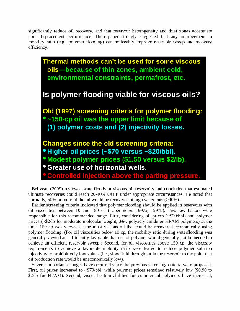
Thermal methods can’t be used for some viscous oils—because of thin zones, ambient cold, environmental constraints, permafrost, etc.

Is polymer flooding viable for viscous oils?

Old (1997) screening criteria for polymer flooding:•~150-cp oil was the upper limit because of

(1) polymer costs and (2) injectivity losses.

Changes since the old screening criteria:•Higher oil prices (~$70 versus ~$20/bbl).•Modest polymer prices ($1.50 versus $2/lb).•Greater use of horizontal wells.•Controlled injection above the parting pressure.

partly from achieving higher polymer molecular weights and partly from incorporating specialty monomers (e.g., with associating groups, Buchgraber et al. 2009) within the polymers. Conventional wisdom from earlier polymer floods was that it was highly desirable to achieve a mobility ratio of unity or less (Maitin 1992). However, with current high oil prices, operators are wondering whether improved sweep from polymer injection might be economically attractive even if a unit mobility ratio is not achieved. In wells that are not fractured, injection of viscous polymer solutions will necessarily decrease injectivity. In order to maintain the waterflood injection rates, the selected polymer-injection wells must allow higher injection pressures. Another important change since the time when earlier screening criteria for polymer flooding were developed (Taber et al. 1997a, 1997b) has been the dramatic increase in the use of horizontal wells. Use of horizontal wells significantly reduces the injectivity restrictions associated with vertical wells, and injector/producer pairs of horizontal wells can improve areal sweep and lessen polymer use requirements (Taber and Seright 1992). Open fractures (either natural or induced) also have a substantial impact on polymer flooding. Waterflooding occurs mostly under induced fracturing conditions (Van den Hoek et al. 2009). Particularly, in low-mobility reservoirs, large fractures may be induced during the field life. Because polymer solutions are more viscous than water, injection above the formation parting pressure will be even more likely during a polymer flood than during a waterflood. The viscoelastic nature (apparent shear-thickening or “pseudo-dilatancy”) for synthetic EOR polymers (e.g., HPAM) makes injection above the formation parting pressure even more likely (Seright 1983, Wang et al. 2008a, Seright et al. 2009c). Under the proper circumstances, injection above the parting pressure can significantly (1) increase polymer solution injectivity and fluid throughput for the reservoir pattern, (2) reduce the risk of mechanical degradation for polyacrylamide solutions, and (3) increase pattern sweep efficiency (Trantham et al. 1980, Wang et al. 2008a, Seright et al. 2009c). Using both field data and theoretical analyses, these facts have been demonstrated at the Daqing Oilfield in China, where the world’s largest polymer flood is in operation (Wang et al. 2008a). Khodaverdian et al. (2009) examined fracture growth during polymer injection into unconsolidated sand formations. During analysis of polymer flooding in this work, we assume that injectivity limitations will require either use of horizontal wells or that polymer injection must occur above the fracture or formation parting pressure. Consequently, linear flow will occur for most of our intended applications. Polymer Flooding Considerations Many factors are important during polymer flooding (Sorbie 1991, Wang et al. 2008b). During design of a polymer flood, critical reservoir factors that traditionally receive consideration are the reservoir lithology, stratigraphy, important heterogeneities (such as fractures), distribution of remaining oil, well pattern, and well distance. Critical polymer properties include cost-effectiveness (e.g., cost per unit of viscosity), resistance to degradation (mechanical/shear, oxidative, thermal, microbial), tolerance of reservoir salinity and hardness, retention by rock, inaccessible pore volume, permeability dependence of performance, rheology, and compatibility with other chemicals that might be used. Issues long recognized as important for polymer bank design include bank size (volume), polymer concentration and salinity (affecting bank viscosity and mobility), and whether (and how) to grade polymer concentrations in the chase water. For brevity, only a few of these factors will be addressed in this report.

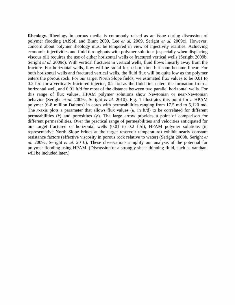
Rheology. Rheology in porous media is commonly raised as an issue during discussion of polymer flooding (AlSofi and Blunt 2009, Lee et al. 2009, Seright et al. 2009c). However, concern about polymer rheology must be tempered in view of injectivity realities. Achieving economic injectivities and fluid throughputs with polymer solutions (especially when displacing viscous oil) requires the use of either horizontal wells or fractured vertical wells (Seright 2009b, Seright et al. 2009c). With vertical fractures in vertical wells, fluid flows linearly away from the fracture. For horizontal wells, flow will be radial for a short time but soon become linear. For both horizontal wells and fractured vertical wells, the fluid flux will be quite low as the polymer enters the porous rock. For our target North Slope fields, we estimated flux values to be 0.01 to 0.2 ft/d for a vertically fractured injector, 0.2 ft/d as the fluid first enters the formation from a horizontal well, and 0.01 ft/d for most of the distance between two parallel horizontal wells. For this range of flux values, HPAM polymer solutions show Newtonian or near-Newtonian behavior (Seright et al. 2009c, Seright et al. 2010). Fig. 1 illustrates this point for a HPAM polymer (6-8 million Daltons) in cores with permeabilities ranging from 17.5 md to 5,120 md. The x-axis plots a parameter that allows flux values (u, in ft/d) to be correlated for different permeabilities (k) and porositites (). The large arrow provides a point of comparison for different permeabilities. Over the practical range of permeabilities and velocities anticipated for our target fractured or horizontal wells (0.01 to 0.2 ft/d), HPAM polymer solutions (in representative North Slope brines at the target reservoir temperature) exhibit nearly constant resistance factors (effective viscosity in porous rock relative to water) (Seright 2009b, Seright et al. 2009c, Seright et al. 2010). These observations simplify our analysis of the potential for polymer flooding using HPAM. (Discussion of a strongly shear-thinning fluid, such as xanthan, will be included later.)

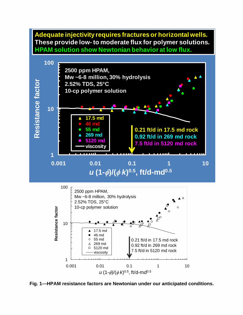
Fig. 1—HPAM resistance factors are Newtonian under our anticipated conditions.

1

10

100

0.001 0.01 0.1 1 10

Res

ista

nce

fac

tor

17.5 md46 md55 md269 md5120 mdviscosity

2500 ppm HPAM,Mw ~6-8 million, 30% hydrolysis 2.52% TDS, 25°C10-cp polymer solution

u (1-)/( k)0.5, ft/d-md0.5

0.21 ft/d in 17.5 md rock0.92 ft/d in 269 md rock7.5 ft/d in 5120 md rock

Adequate injectivity requires fractures or horizontal wells. These provide low- to moderate flux for polymer solutions.HPAM solution show Newtonian behavior at low flux.

1

10

100

0.001 0.01 0.1 1 10

Res

ista

nce

fac

tor

17.5 md46 md55 md269 md5120 mdviscosity

2500 ppm HPAM,Mw ~6-8 million, 30% hydrolysis 2.52% TDS, 25°C10-cp polymer solution

u (1-)/( k)0.5, ft/d-md0.5

0.21 ft/d in 17.5 md rock0.92 ft/d in 269 md rock7.5 ft/d in 5120 md rock

Permeability Dependence of Resistance Factors. Many studies (Chauveteau 1982, Cannella et al. 1988, Seright 1991) showed that resistance factor correlated quite well using the parameter u(1-)/(k)0.5, where u is flux (in ft/d), is porosity, and k is permeability (in md). This effect is also demonstrated in Fig. 1. Beyond this rheological effect, polymers of a given type and molecular weight are known to exhibit a permeability, below which they experience difficulty in propagating through porous rock (Jenning et al. 1971, Vela et al. 1976, Zhang and Seright 2007, Wang et al. 2008b, Wang et al. 2009). As permeability decreases below this critical value, resistance factors, residual resistance factors, and polymer retention increase dramatically. As recommended by Wang et al. (2008b, 2009), we assume that the molecular weight and size of the chosen polymer are small enough so that the polymer will propagate effectively through all permeabilities and layers of interest—so this internal pore-plugging effect does not occur. A later section, “Practical Impact of Permability Reduction and Its Variation with Permeability,” will consider the effect of different resistance factors in different layers. Gravity. For the viscous crudes that we target, the density difference () between water and oil is relatively small (12-23° API, 0.986 to 0.916 g/cm3 oil density, with perhaps =0.05 g/cm3 being typical between oil and water). An estimate of the vertical flux of a polymer front can be made using the gravity portion of the Darcy equation. Assuming a density difference of 0.05 g/cm3, a reservoir permeability of 100 md, and injection of a 10-cp polymer solution, the vertical migration of the polymer front due to gravity will only be about 6 inches per year (Seright 2009b). Consequently, gravity effects will be neglected in our subsequent considerations and calculations. Our work also assumes incompressible and isothermal conditions. Reduction of Residual Oil Saturation. Some reports indicate that polymer solutions can reduce the residual oil saturation (Sor) below values expected for extensive waterflooding, and thereby increase the relative permeability to water (Wu et al. 2007, Huh and Pope 2008). Although we are currently experimentally exploring this issue for North Slope oil and conditions, this report will assume that the same Sor value would ultimately be attained with either waterflooding or polymer flooding. Simulation versus Fractional Flow Calculations. Simulation studies of polymer flooding are valuable in that complex reservoir configurations and combined effects of multiple physical, chemical, and fluid phenomena can be examined. Of course, inappropriate assumptions can lead to unrealistic predictions. Unfortunately, if a commercial simulator is used by someone who is not intimately familiar with the assumptions or defaults that are inherent in the software, flaws in the output may not be readily apparent. Three examples are mentioned here that have been witnessed recently. First, if the simulator incorrectly assumes shear-thinning behavior for an HPAM polymer, an overly optimistic injectivity will be predicted (Seright et al. 2009c). Second, if crossflow is not initiated properly in the simulator, recovery values can be incorrectly predicted to be similar to no-crossflow cases, even though the mobility ratio is nowhere near unity (Seright 2009b). Third, an unconventional definition of inaccessible pore volume can confuse one to enter a grossly inappropriate value (Dawson and Lantz 1972). As an alternative to simulation, fractional flow analysis was used by several authors to quantify polymer flood performance (Lake 1989, Sorbie 1991, Green and Willhite 1998). This type of analysis has the advantage of being sufficiently transparent to readily determine whether the

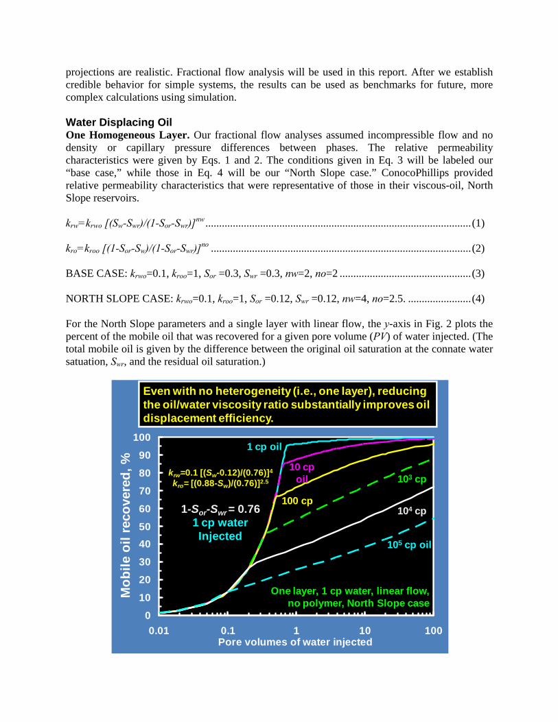
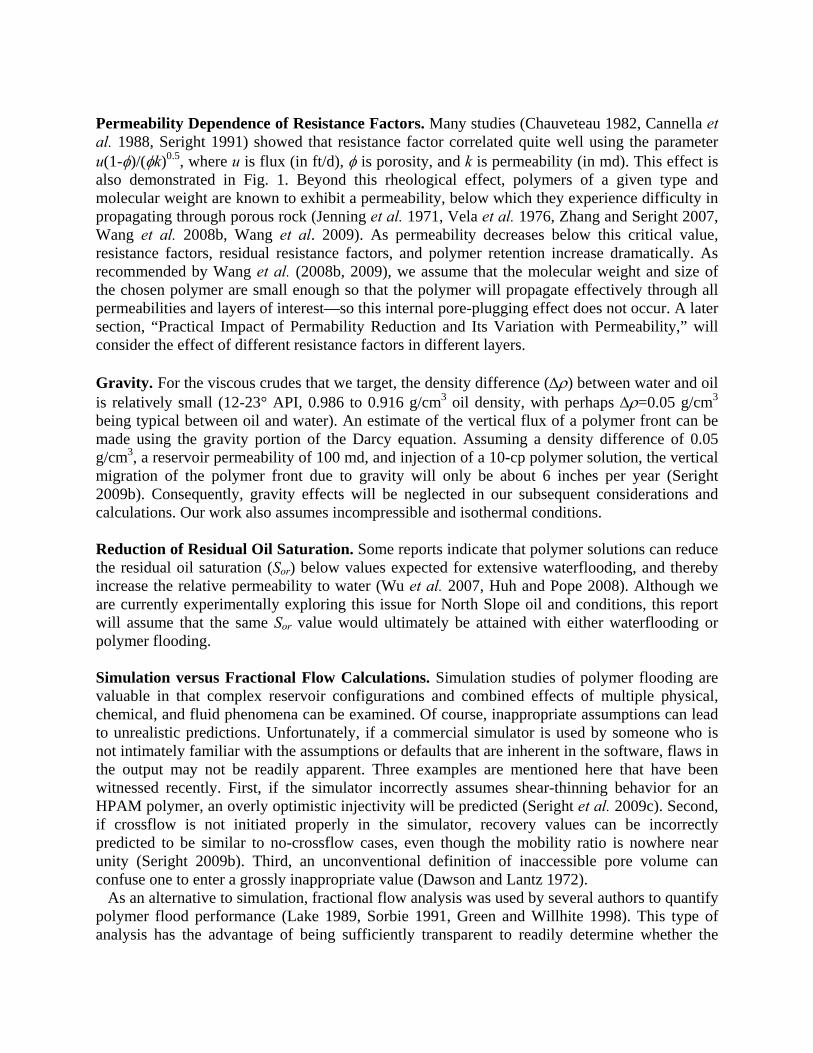
projections are realistic. Fractional flow analysis will be used in this report. After we establish credible behavior for simple systems, the results can be used as benchmarks for future, more complex calculations using simulation. Water Displacing Oil One Homogeneous Layer. Our fractional flow analyses assumed incompressible flow and no density or capillary pressure differences between phases. The relative permeability characteristics were given by Eqs. 1 and 2. The conditions given in Eq. 3 will be labeled our “base case,” while those in Eq. 4 will be our “North Slope case.” ConocoPhillips provided relative permeability characteristics that were representative of those in their viscous-oil, North Slope reservoirs. krw=krwo [(Sw-Swr)/(1-Sor-Swr)]

nw ................................................................................................. (1) kro=kroo [(1-Sor-Sw)/(1-Sor-Swr)]

no ............................................................................................... (2) BASE CASE: krwo=0.1, kroo=1, Sor =0.3, Swr =0.3, nw=2, no=2 ................................................ (3) NORTH SLOPE CASE: krwo=0.1, kroo=1, Sor =0.12, Swr =0.12, nw=4, no=2.5. ....................... (4) For the North Slope parameters and a single layer with linear flow, the y-axis in Fig. 2 plots the percent of the mobile oil that was recovered for a given pore volume (PV) of water injected. (The total mobile oil is given by the difference between the original oil saturation at the connate water satuation, Swr, and the residual oil saturation.)

0

10

20

30

40

50

60

70

80

90

100

0.01 0.1 1 10 100Pore volumes of water injected

Mo

bil

e o

il r

eco

vere

d,

%

1 cp oil

10 cp oil

100 cp

One layer, 1 cp water, linear flow, no polymer, North Slope case

krw=0.1 [(Sw-0.12)/(0.76)]4

kro= [(0.88-Sw)/(0.76)]2.5

1-Sor-Swr = 0.761 cp waterInjected

103 cp

104 cp

105 cp oil

Even with no heterogeneity (i.e., one layer), reducing the oil/water viscosity ratio substantially improves oil displacement efficiency.

Fig. 2—Fractional flow calculations for water displacing oil, one layer. North

Slope case.

Two Layers with/without Crossflow. For the next set of cases, we considered linear displacement through two layers (of equal thickness), where k1=1 darcy, ϕ1=0.3, k2=0.1 darcy, ϕ2=0.3. All other parameters and conditions were the same as those used in the one-layer case. We considered two subsets—one with no crossflow between the two layers and one with free crossflow (i.e., vertical equilibrium) between the layers. For the two-layer cases, we solved the fractional flow calculations using spreadsheets. The two-layer no-crossflow case was straight forward, since the displacements in the individual layers can be treated separately and then combined to yield the overall displacement efficiency (Green and Willhite 1998). The free-crossflow case required application of vertical equilibrium between the layers (Zapata and Lake 1981, Lake 1989). Examples of these spreadsheets can be found at Seright 2009a. Based on the fractional flow calculations for various crossflow and no-crossflow cases, Table 1 lists the recovery values at 1 PV of water injection, for relative permeabilites associated with both our base case and North Slope case. Along with Fig. 2, this table hints at the potential for polymer flooding. For any given oil viscosity (e.g., 1,000 cp), one can envision that a 10-fold decrease in the oil/water viscosity ratio (i.e., injecting a 10-cp polymer solution instead of water) could increase oil recovery by a substantial percentage. Accepted reservoir engineering analysis indicates two key expectations (Coats et al. 1971, Craig 1971, Zapata and Lake 1981, Sorbie and Seright 1992). First, as the mobility ratio becomes increasingly small (below unity), the vertical sweep efficiency increases for both the crossflow and no-crossflow cases. However, the crossflow cases achieve much higher recovery efficiencies than the no-crossflow cases. Second, as the mobility ratio becomes increasingly large (above unity), the sweep efficiency decreases for both the crossflow and no-crossflow cases. However, the crossflow cases suffer lower recovery efficiencies than the no-crossflow cases. To restate, crossflow cases lose efficiency much faster than the no-crossflow cases as the mobility ratio increases. These expections are confirmed in Table 1. For 1-cp water displacing 1-cp oil in

0

10

20

30

40

50

60

70

80

90

100


Mo

bile

oil

reco

vere

d,

%

1 cp oil

10 cp oil

100 cp

1-Sor-Swr = 0.761 cp waterinjected

103 cp

104 cp

105 cp oil

a two-layer reservoir, oil recoveries were higher for the crossflow cases than for the no-crossflow cases—because the mobility ratios were favorable during the displacement. For 1-cp water displacing 10-cp oil, oil recoveries were about the same for the crossflow and no-crossflow cases—because the mobility ratios were near unity during the displacement. For the 1-cp water displacing more viscous oils, oil recoveries were less for the crossflow cases than for the no-crossflow cases—because the mobility ratios were unfavorable during the displacement.

Table 1—% mobile oil recovered after 1 PV of 1-cp water injection. Oil

viscosity, cp

1 layer 2 layers, no crossflow

2 layers with crossflow

Base case

North Slope case

Base case

North Slope case

Base case

North Slope case

1 99 96 98 76 99 96 10 92 87 70 57 62 58

100 70 72 62 50 43 41 1,000 43 54 38 41 27 30

10,000 22 38 20 33 14 22 100,000 11 25 10 23 7 15

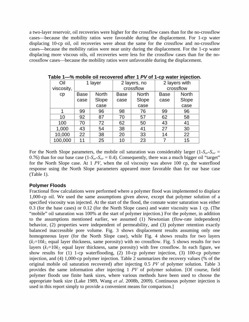
For the North Slope parameters, the mobile oil saturation was considerably larger (1-Sor-Swr = 0.76) than for our base case (1-Sor-Swr = 0.4). Consequently, there was a much bigger oil “target” for the North Slope case. At 1 PV, when the oil viscosity was above 100 cp, the waterflood response using the North Slope parameters appeared more favorable than for our base case (Table 1). Polymer Floods Fractional flow calculations were performed where a polymer flood was implemented to displace 1,000-cp oil. We used the same assumptions given above, except that polymer solution of a specified viscosity was injected. At the start of the flood, the connate water saturation was either 0.3 (for the base cases) or 0.12 (for the North Slope cases) and water viscosity was 1 cp. (The “mobile” oil saturation was 100% at the start of polymer injection.) For the polymer, in addition to the assumptions mentioned earlier, we assumed (1) Newtonian (flow-rate independent) behavior, (2) properties were independent of permeability, and (3) polymer retention exactly balanced inaccessible pore volume. Fig. 3 shows displacement results assuming only one homogeneous layer (for the North Slope case), while Fig. 4 shows results for two layers (k1=10k2, equal layer thickness, same porosity) with no crossflow. Fig. 5 shows results for two layers (k1=10k2, equal layer thickness, same porosity) with free crossflow. In each figure, we show results for (1) 1-cp waterflooding, (2) 10-cp polymer injection, (3) 100-cp polymer injection, and (4) 1,000-cp polymer injection. Table 2 summarizes the recovery values (% of the original mobile oil saturation recovered) after injecting 0.5 PV of polymer solution. Table 3 provides the same information after injecting 1 PV of polymer solution. [Of course, field polymer floods use finite bank sizes, where various methods have been used to choose the appropriate bank size (Lake 1989, Wang et al. 2008b, 2009). Continuous polymer injection is used in this report simply to provide a convenient means for comparison.]

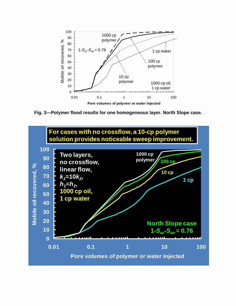
Fig. 3—Polymer flood results for one homogeneous layer. North Slope case.

0

10

20

30

40

50

60

70

80

90

100

0.01 0.1 1 10 100

Pore volumes of polymer or water injected

Mo

bile

oil

reco

vere

d,

%

10 cp polymer

1 cp water

1000 cp oil, 1 cp water

1000 cp polymer

100 cp polymer

1-Sor-Swr = 0.76

0

10

20

30

40

50

60

70

80

90

100

0.01 0.1 1 10 100


Mo

bile

oil

rec

ov

ere

d, %

1000 cp polymer 100 cp

10 cp

1 cp

Two layers, no crossflow,linear flow,k1=10k2, h1=h2,1000 cp oil, 1 cp water

North Slope case1-Sor-Swr = 0.76

For cases with no crossflow, a 10-cp polymer solution provides noticeable sweep improvement.

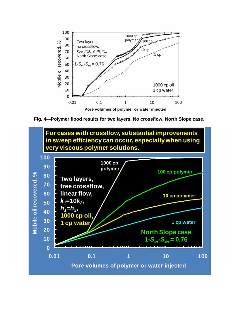
Fig. 4—Polymer flood results for two layers. No crossflow. North Slope case.

0

10

20

30

40

50

60

70

80

90

100

0.01 0.1 1 10 100


Mo

bile

oil

reco

vere

d,

%

1000 cp polymer 100 cp

10 cp

1 cp

1000 cp oil1 cp water

1-Sor-Swr = 0.76

Two-layers, no crossflow, k1/k2=10, h1/h2=1,North Slope case

0

10

20

30

40

50

60

70

80

90

100

0.01 0.1 1 10 100


Mo

bile

oil

rec

ov

ere

d, %

10 cp polymer

1 cp water

1000 cp polymer

100 cp polymer

Two layers, free crossflow,linear flow,k1=10k2, h1=h2,1000 cp oil, 1 cp water

For cases with crossflow, substantial improvements in sweep efficiency can occur, especially when using very viscous polymer solutions.

North Slope case1-Sor-Swr = 0.76

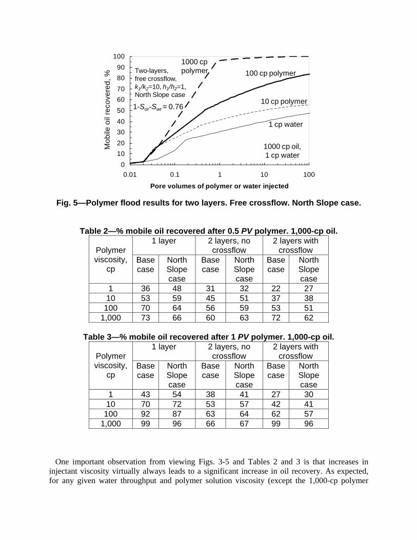
Fig. 5—Polymer flood results for two layers. Free crossflow. North Slope case.

Table 2—% mobile oil recovered after 0.5 PV polymer. 1,000-cp oil.

Polymer viscosity,

cp



Base case

North Slope case

Base case

North Slope case

Base case

North Slope case

1 36 48 31 32 22 27 10 53 59 45 51 37 38

100 70 64 56 59 53 51 1,000 73 66 60 63 72 62

Table 3—% mobile oil recovered after 1 PV polymer. 1,000-cp oil.

Polymer viscosity,

cp



Base case

North Slope case

Base case

North Slope case

Base case

North Slope case

1 43 54 38 41 27 30 10 70 72 53 57 42 41

100 92 87 63 64 62 57 1,000 99 96 66 67 99 96

One important observation from viewing Figs. 3-5 and Tables 2 and 3 is that increases in injectant viscosity virtually always leads to a significant increase in oil recovery. As expected, for any given water throughput and polymer solution viscosity (except the 1,000-cp polymer

0

10

20

30

40

50

60

70

80

90

100

0.01 0.1 1 10 100


Mo

bile

oil

reco

vere

d,

%10 cp polymer

1 cp water


1000 cp polymer 100 cp polymer

1-Sor-Swr = 0.76

Two-layers, free crossflow, k1/k2=10, h1/h2=1,North Slope case

cases), recovery efficiency was substantially better for the one-layer cases (Fig. 3) than for the two-layer cases (Figs. 4 and 5). Interestingly, the recovery curves when injecting 1,000-cp polymer solution were quite similar for both the one-layer cases and two-layer cases with free crossflow (thick dashed curves in Fig. 3 versus Fig. 5). This finding is consistent with vertical equilibrium concepts. If the mobility contrast between the displacing and displaced phases [i.e., (1 darcy kro/1,000-cp oil)/(0.1 darcy krw/1,000-cp polymer)=10] is greater than or equal to the permeability contrast (i.e., k1/k2=10), then the displacement efficiency for two layers will appear the same as for one layer (Sorbie and Seright 1992). For the one-layer cases and the two-layer cases with free crossflow, the waterfloods (i.e., 1-cp polymer) were noticeably more efficient (by 3-12% of the mobile oil) for the North Slope conditions than the base case (see the first data rows of Tables 2 and 3). For the two-layer cases with no crossflow, the waterflood recoveries were quite similar for the North Slope and base cases (32% versus 31% after 0.5 PV and 41% versus 38% after 1 PV). At any given injection volume for the cases with no crossflow, the largest increases in recovery generally occurred when increasing the injectant viscosity from 1 cp to 10 cp (Fig. 4). For the cases with free crossflow (Fig. 5), the largest increase in recovery occurred when increasing the injectant viscosity from 100 to 1,000 cp. Most previous field polymer floods were directed at reservoirs with oil/water viscosity ratios that were less than 10, although the most successful projects had ratios from 15 to 114 (Taber et al. 1997b). For the world’s largest (and most definitive) polymer flood at Daqing, China, the oil/water viscosity ratio was 15, and 10-12% of the original oil in place (OOIP) was recovered, incremental over waterflooding (Wang et al. 1995, Taber et al. 1997b, Wang et al. 2008b, Wang et al. 2009).

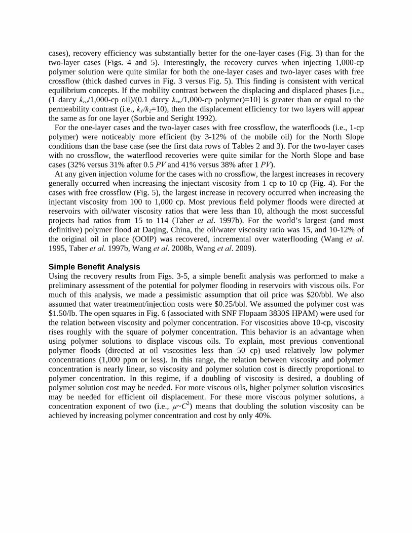
Simple Benefit Analysis Using the recovery results from Figs. 3-5, a simple benefit analysis was performed to make a preliminary assessment of the potential for polymer flooding in reservoirs with viscous oils. For much of this analysis, we made a pessimistic assumption that oil price was $20/bbl. We also assumed that water treatment/injection costs were $0.25/bbl. We assumed the polymer cost was $1.50/lb. The open squares in Fig. 6 (associated with SNF Flopaam 3830S HPAM) were used for the relation between viscosity and polymer concentration. For viscosities above 10-cp, viscosity rises roughly with the square of polymer concentration. This behavior is an advantage when using polymer solutions to displace viscous oils. To explain, most previous conventional polymer floods (directed at oil viscosities less than 50 cp) used relatively low polymer concentrations (1,000 ppm or less). In this range, the relation between viscosity and polymer concentration is nearly linear, so viscosity and polymer solution cost is directly proportional to polymer concentration. In this regime, if a doubling of viscosity is desired, a doubling of polymer solution cost may be needed. For more viscous oils, higher polymer solution viscosities may be needed for efficient oil displacement. For these more viscous polymer solutions, a concentration exponent of two (i.e., µ~C2) means that doubling the solution viscosity can be achieved by increasing polymer concentration and cost by only 40%.

Fig. 6—Viscosity versus polymer concentration.

1

10

100

1000

10000

100 1000 10000 100000

Polymer concentration, ppm

Vis

co

sit

y @

7.3

s-1

, cp

diutan

xanthan19 million Mw HPAM

7 million Mw HPAM

Polymers are more efficient viscosifiers at high concentrations: µ ~ C2 (i.e., only 40% more polymer is needed to double the viscosity).

polymer in 2.52% TDS brine, 25ºC

Most previouspolymer floods

Viscous oilpolymer floods

1

10

100

1000

10000

100 1000 10000 100000

Polymer concentration, ppm

Vis

cosi

ty @

7.3

s-1

, cp

diutan

xanthan

19 million Mw HPAM

7 million Mw HPAM

polymer in 2.52% TDS brine

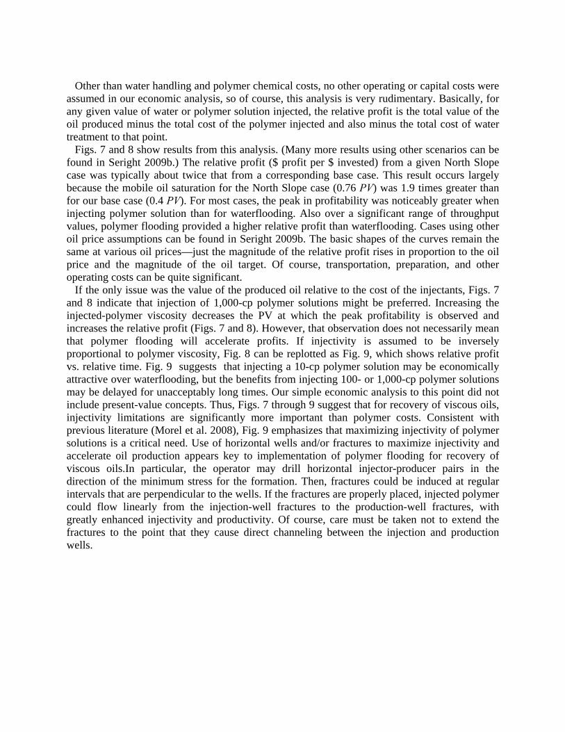
Other than water handling and polymer chemical costs, no other operating or capital costs were assumed in our economic analysis, so of course, this analysis is very rudimentary. Basically, for any given value of water or polymer solution injected, the relative profit is the total value of the oil produced minus the total cost of the polymer injected and also minus the total cost of water treatment to that point. Figs. 7 and 8 show results from this analysis. (Many more results using other scenarios can be found in Seright 2009b.) The relative profit ($ profit per $ invested) from a given North Slope case was typically about twice that from a corresponding base case. This result occurs largely because the mobile oil saturation for the North Slope case (0.76 PV) was 1.9 times greater than for our base case (0.4 PV). For most cases, the peak in profitability was noticeably greater when injecting polymer solution than for waterflooding. Also over a significant range of throughput values, polymer flooding provided a higher relative profit than waterflooding. Cases using other oil price assumptions can be found in Seright 2009b. The basic shapes of the curves remain the same at various oil prices—just the magnitude of the relative profit rises in proportion to the oil price and the magnitude of the oil target. Of course, transportation, preparation, and other operating costs can be quite significant. If the only issue was the value of the produced oil relative to the cost of the injectants, Figs. 7 and 8 indicate that injection of 1,000-cp polymer solutions might be preferred. Increasing the injected-polymer viscosity decreases the PV at which the peak profitability is observed and increases the relative profit (Figs. 7 and 8). However, that observation does not necessarily mean that polymer flooding will accelerate profits. If injectivity is assumed to be inversely proportional to polymer viscosity, Fig. 8 can be replotted as Fig. 9, which shows relative profit vs. relative time. Fig. 9 suggests that injecting a 10-cp polymer solution may be economically attractive over waterflooding, but the benefits from injecting 100- or 1,000-cp polymer solutions may be delayed for unacceptably long times. Our simple economic analysis to this point did not include present-value concepts. Thus, Figs. 7 through 9 suggest that for recovery of viscous oils, injectivity limitations are significantly more important than polymer costs. Consistent with previous literature (Morel et al. 2008), Fig. 9 emphasizes that maximizing injectivity of polymer solutions is a critical need. Use of horizontal wells and/or fractures to maximize injectivity and accelerate oil production appears key to implementation of polymer flooding for recovery of viscous oils.In particular, the operator may drill horizontal injector-producer pairs in the direction of the minimum stress for the formation. Then, fractures could be induced at regular intervals that are perpendicular to the wells. If the fractures are properly placed, injected polymer could flow linearly from the injection-well fractures to the production-well fractures, with greatly enhanced injectivity and productivity. Of course, care must be taken not to extend the fractures to the point that they cause direct channeling between the injection and production wells.

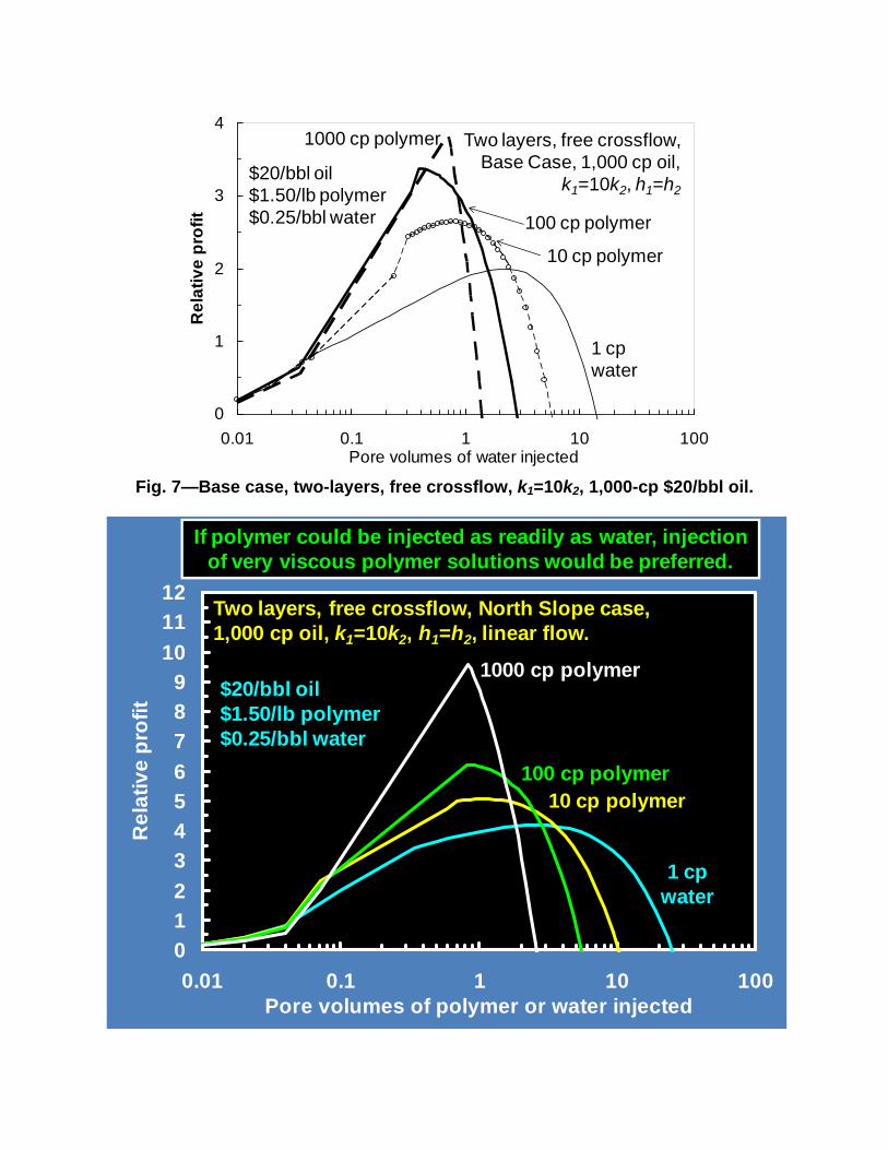
Fig. 7—Base case, two-layers, free crossflow, k1=10k2, 1,000-cp $20/bbl oil.

0

1

2

3

4


Re

lati

ve

pro

fit

Two layers, free crossflow,Base Case, 1,000 cp oil,

k1=10k2, h1=h2

1 cpwater

$20/bbl oil$1.50/lb polymer$0.25/bbl water

10 cp polymer

100 cp polymer

1000 cp polymer

0

1

2

3

4

5

6

7

8

9

10

11

12

0.01 0.1 1 10 100Pore volumes of polymer or water injected

Re

lati

ve

pro

fit

1 cp water


10 cp polymer100 cp polymer

If polymer could be injected as readily as water, injection of very viscous polymer solutions would be preferred.

1000 cp polymer

Two layers, free crossflow, North Slope case,1,000 cp oil, k1=10k2, h1=h2, linear flow.

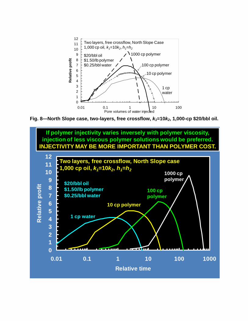
Fig. 8—North Slope case, two-layers, free crossflow, k1=10k2, 1,000-cp $20/bbl oil.

0

1

2

3

4

5

6

7

8

9

10

11

12


Re

lati

ve

pro

fit

Two layers, free crossflow, North Slope Case1,000 cp oil, k1=10k2, h1=h2

1 cpwater


10 cp polymer

100 cp polymer

1000 cp polymer

0123456789

101112

0.01 0.1 1 10 100 1000

Relative time

Re

lati

ve

pro

fit

1 cp water


10 cp polymer

100 cp polymer

1000 cp polymer

Two layers, free crossflow, North Slope case1,000 cp oil, k1=10k2, h1=h2

If polymer injectivity varies inversely with polymer viscosity, injection of less viscous polymer solutions would be preferred.

INJECTIVITY MAY BE MORE IMPORTANT THAN POLYMER COST.

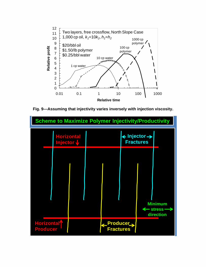
Fig. 9—Assuming that injectivity varies inversely with injection viscosity.

0123456789

101112

0.01 0.1 1 10 100 1000

Relative time

Re

lati

ve

pro

fit

Two layers, free crossflow, North Slope Case1,000 cp oil, k1=10k2, h1=h2

1 cp water


100 cp polymer

1000 cppolymer

10 cp water

Scheme to Maximize Polymer Injectivity/Productivity

Horizontal Injector

Horizontal Producer

InjectorFractures

ProducerFractures

Minimumstress

direction

Practical Impact of Permeability Reduction and Its Variation with Permeability In the work to this point, we assumed that the polymer reduced mobility simply by increasing solution viscosity. Also, we assumed that the effective polymer solution viscosity (resistance factor) was the same in all layers, regardless of permeability. Early work (Pye 1964, Smith 1970, Jennings et al. 1971, Hirasaki and Pope 1974) recognized that high molecular weight HPAM sometimes reduced the mobility ( or k/) of aqueous solutions in porous media by a greater factor than can be rationalized based on the viscosity (µ) of the solution. The incremental reduction in mobility was attributed to reduction in permeability (k), caused by adsorption or mechanical entrapment of the high molecular weight polymers—especially from the largest polymers in the molecular weight distribution for a given polymer. In the 1960s and 1970s, this effect was touted to be of great benefit (Pye 1964, Jennings et al. 1971) for polymer floods (simply because the polymer appeared to provide significantly more apparent viscosity in porous media than expected from normal viscosity measurements). However, these benefits were often not achievable in field applications because normal field handling and flow through an injection sand face at high velocities mechanically degraded the large molecules that were responsible for the permeability reduction (Seright et al. 1981, Seright 1983, Seright et al. 2010). Also, the largest molecules were expected to be preferentially retained (i.e., by mechanical entrapment in pores) and stripped from the polymer solution before penetrating deep into the formation (Seright et al. 2010).

Even if high permeability reductions could be achieved, would this effect actually be of benefit? More specifically, the concern focuses on how the mobility reduction varies with permeability of porous media. For adsorbed polymers, resistance factors (Fr, apparent viscosities in porous media relative to brine) and residual resistance factors (Frr, permeability reduction values) increase with decreasing permeability (Pye 1964, Jennings et al. 1971, Hirasaki and Pope 1974, Vela et al. 1976, Jewett and Schurz 1979, Zaitoun and Kohler 1988, Rousseau et al. 2005). In other words, these polymers can reduce the flow capacity of low permeability rock by a greater factor than high permeability rock. Depending on the magnitude of this effect, these polymers and gels can harm vertical flow profiles in wells, even though the polymer penetrates significantly farther into the high permeability rock (Seright 1988, Seright 1991, Liang et al. 1993, Zhang and Seright 2007).

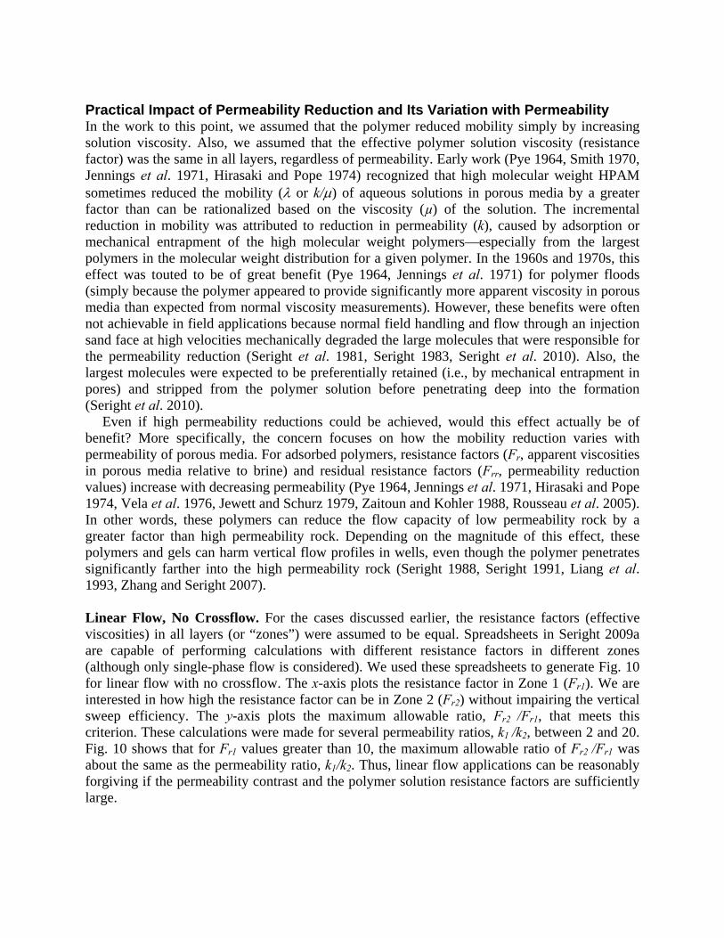
Linear Flow, No Crossflow. For the cases discussed earlier, the resistance factors (effective viscosities) in all layers (or “zones”) were assumed to be equal. Spreadsheets in Seright 2009a are capable of performing calculations with different resistance factors in different zones (although only single-phase flow is considered). We used these spreadsheets to generate Fig. 10 for linear flow with no crossflow. The x-axis plots the resistance factor in Zone 1 (Fr1). We are interested in how high the resistance factor can be in Zone 2 (Fr2) without impairing the vertical sweep efficiency. The y-axis plots the maximum allowable ratio, Fr2 /Fr1, that meets this criterion. These calculations were made for several permeability ratios, k1 /k2, between 2 and 20. Fig. 10 shows that for Fr1 values greater than 10, the maximum allowable ratio of Fr2 /Fr1 was about the same as the permeability ratio, k1/k2. Thus, linear flow applications can be reasonably forgiving if the permeability contrast and the polymer solution resistance factors are sufficiently large.

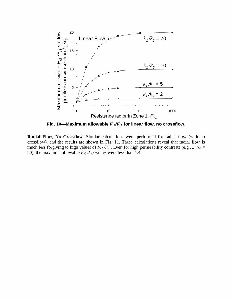
Fig. 10—Maximum allowable Fr2/Fr1 for linear flow, no crossflow.

Radial Flow, No Crossflow. Similar calculations were performed for radial flow (with no crossflow), and the results are shown in Fig. 11. These calculations reveal that radial flow is much less forgiving to high values of Fr2 /Fr1. Even for high permeability contrasts (e.g., k1 /k2 = 20), the maximum allowable Fr2 /Fr1 values were less than 1.4.

0

5

10

15

20

1 10 100 1000

Resistance factor in Zone 1, F r1

k1 /k2 = 20

Max

imum

allo

wa

ble

Fr2

/F

r1so

flo

wpr

ofile

is n

o w

ors

e th

ank 1

/k2

k1 /k2 = 10

k1 /k2 = 5

k1 /k2 = 2

Linear Flow

Fig. 11—Maximum allowable Fr2/Fr1 for radial flow, no crossflow.

1

1.1

1.2

1.3

1.4

1.5

1 10 100 1000

Resistance factor in Zone 1

k1/k2= 20

k1/k2= 10

k1/k2= 5

k1/k2= 2

Max

imu

m a

llo

wab

le r

esis

tan

ce fa

cto

r in

Zo

ne

2 (r

elat

ive

to th

at in

Zo

ne

1) t

o a

chie

ve v

erti

cal

swee

p n

o w

ors

e th

an fo

r a

wat

er fl

oo

d

For polymers, Fr values often increase with decreasing k.What if Fr1 Fr2? For radial flow, Fr2 must be < 1.4 Fr1.

No crossflow case, Radial flow.

1

1.1

1.2

1.3

1.4

1 10 100 1000

Resistance factor in Zone 1, F r1

k1 /k2 = 20

Max

imum

allo

wa

ble

Fr2

/F

r1so

flo

wpr

ofile

is n

o w

ors

e th

ank 1

/k2

k1 /k2 = 10

k1 /k2 = 5

k1 /k2 = 2

Radial Flow

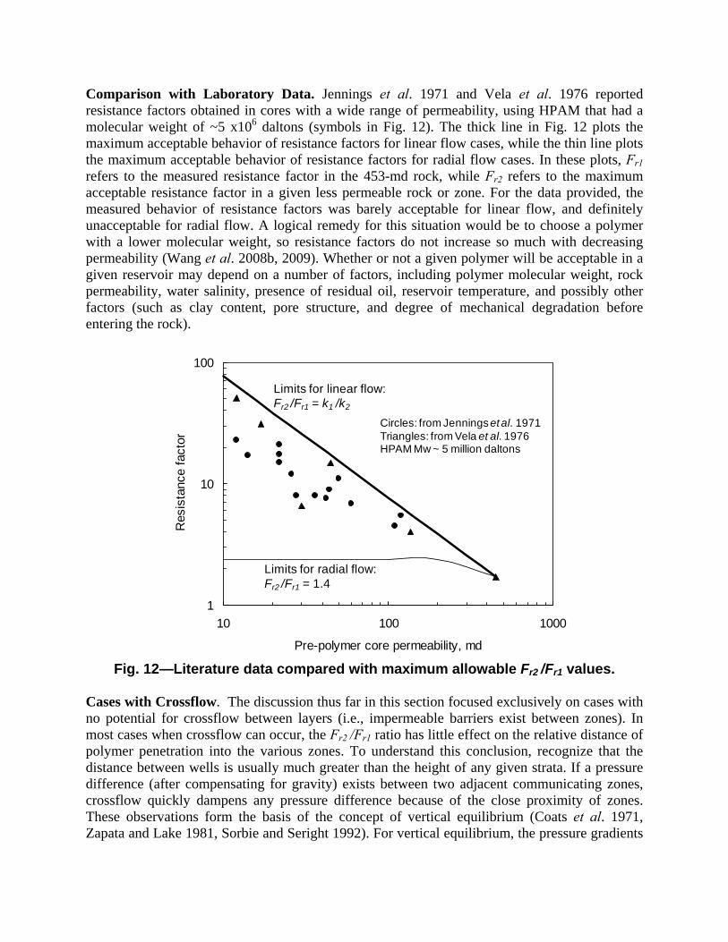
Comparison with Laboratory Data. Jennings et al. 1971 and Vela et al. 1976 reported resistance factors obtained in cores with a wide range of permeability, using HPAM that had a molecular weight of ~5 x106 daltons (symbols in Fig. 12). The thick line in Fig. 12 plots the maximum acceptable behavior of resistance factors for linear flow cases, while the thin line plots the maximum acceptable behavior of resistance factors for radial flow cases. In these plots, Fr1 refers to the measured resistance factor in the 453-md rock, while Fr2 refers to the maximum acceptable resistance factor in a given less permeable rock or zone. For the data provided, the measured behavior of resistance factors was barely acceptable for linear flow, and definitely unacceptable for radial flow. A logical remedy for this situation would be to choose a polymer with a lower molecular weight, so resistance factors do not increase so much with decreasing permeability (Wang et al. 2008b, 2009). Whether or not a given polymer will be acceptable in a given reservoir may depend on a number of factors, including polymer molecular weight, rock permeability, water salinity, presence of residual oil, reservoir temperature, and possibly other factors (such as clay content, pore structure, and degree of mechanical degradation before entering the rock).

Fig. 12—Literature data compared with maximum allowable Fr2 /Fr1 values.

Cases with Crossflow. The discussion thus far in this section focused exclusively on cases with no potential for crossflow between layers (i.e., impermeable barriers exist between zones). In most cases when crossflow can occur, the Fr2 /Fr1 ratio has little effect on the relative distance of polymer penetration into the various zones. To understand this conclusion, recognize that the distance between wells is usually much greater than the height of any given strata. If a pressure difference (after compensating for gravity) exists between two adjacent communicating zones, crossflow quickly dampens any pressure difference because of the close proximity of zones. These observations form the basis of the concept of vertical equilibrium (Coats et al. 1971, Zapata and Lake 1981, Sorbie and Seright 1992). For vertical equilibrium, the pressure gradients

1

10

100

10 100 1000

Pre-polymer core permeability, md

Res

ista

nce

fact

or

Limits for radial flow:Fr2 /Fr1 = 1.4

Limits for linear flow:Fr2 /Fr1 = k1 /k2

Circles: from Jennings et al. 1971Triangles: from Vela et al. 1976HPAM Mw ~ 5 million daltons

in two adjacent zones (with no flow barriers) are the same for any given horizontal position. Put another way, for a given distance from the wellbore (if gravity can be neglected), the pressure is the same in both zones.

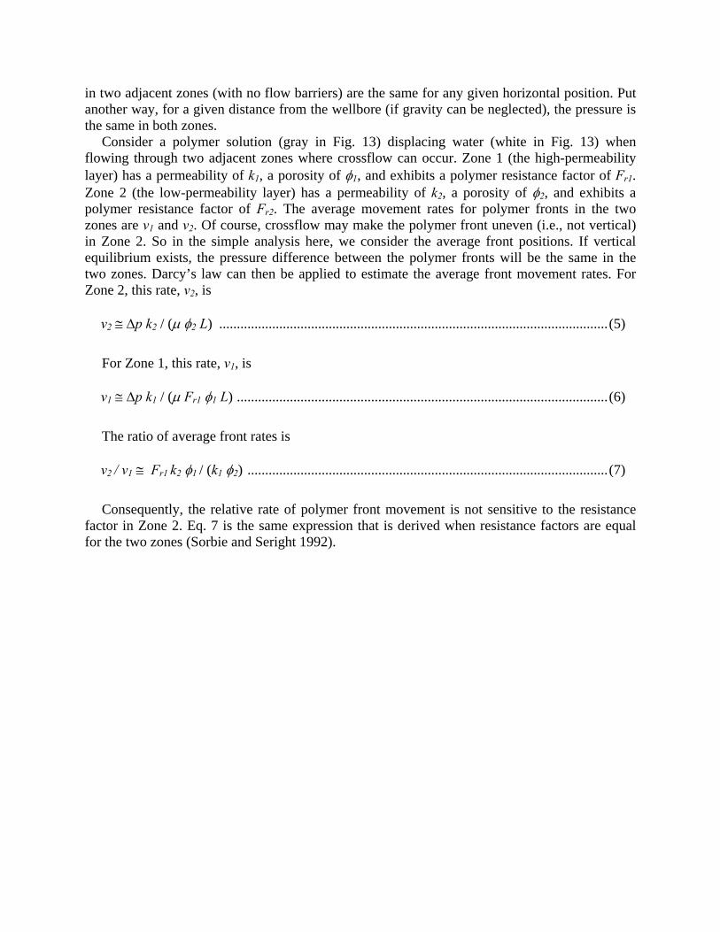
Consider a polymer solution (gray in Fig. 13) displacing water (white in Fig. 13) when flowing through two adjacent zones where crossflow can occur. Zone 1 (the high-permeability layer) has a permeability of k1, a porosity of 1, and exhibits a polymer resistance factor of Fr1. Zone 2 (the low-permeability layer) has a permeability of k2, a porosity of 2, and exhibits a polymer resistance factor of Fr2. The average movement rates for polymer fronts in the two zones are v1 and v2. Of course, crossflow may make the polymer front uneven (i.e., not vertical) in Zone 2. So in the simple analysis here, we consider the average front positions. If vertical equilibrium exists, the pressure difference between the polymer fronts will be the same in the two zones. Darcy’s law can then be applied to estimate the average front movement rates. For Zone 2, this rate, v2, is

v2 p k2 / ( 2 L) .............................................................................................................. (5)

For Zone 1, this rate, v1, is

v1 p k1 / ( Fr1 1 L) ......................................................................................................... (6)

The ratio of average front rates is

v2 / v1 Fr1 k2 1 / (k1 2) ...................................................................................................... (7)

Consequently, the relative rate of polymer front movement is not sensitive to the resistance factor in Zone 2. Eq. 7 is the same expression that is derived when resistance factors are equal for the two zones (Sorbie and Seright 1992).

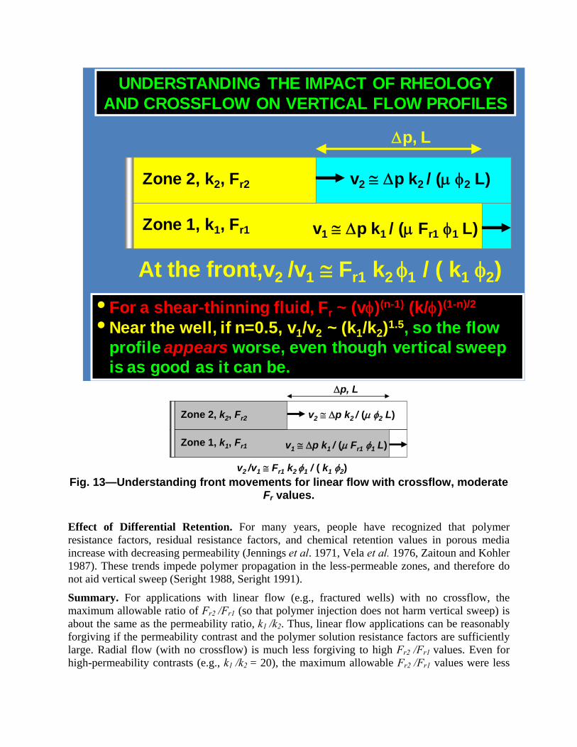
Fig. 13—Understanding front movements for linear flow with crossflow, moderate

Fr values.

Effect of Differential Retention. For many years, people have recognized that polymer resistance factors, residual resistance factors, and chemical retention values in porous media increase with decreasing permeability (Jennings et al. 1971, Vela et al. 1976, Zaitoun and Kohler 1987). These trends impede polymer propagation in the less-permeable zones, and therefore do not aid vertical sweep (Seright 1988, Seright 1991).

Summary. For applications with linear flow (e.g., fractured wells) with no crossflow, the maximum allowable ratio of Fr2 /Fr1 (so that polymer injection does not harm vertical sweep) is about the same as the permeability ratio, k1 /k2. Thus, linear flow applications can be reasonably forgiving if the permeability contrast and the polymer solution resistance factors are sufficiently large. Radial flow (with no crossflow) is much less forgiving to high Fr2 /Fr1 values. Even for high-permeability contrasts (e.g., k1 /k2 = 20), the maximum allowable Fr2 /Fr1 values were less

Zone 2, k2, Fr2

At the front,v2 /v1 Fr1 k2 1 / ( k1 2)

Zone 1, k1, Fr1

p, L

v2 p k2 / ( 2 L)

v1 p k1 / ( Fr1 1 L)

UNDERSTANDING THE IMPACT OF RHEOLOGY AND CROSSFLOW ON VERTICAL FLOW PROFILES

• For a shear-thinning fluid, Fr ~ (v)(n-1) (k/)(1-n)/2

• Near the well, if n=0.5, v1/v2 ~ (k1/k2)1.5, so the flow profile appears worse, even though vertical sweep is as good as it can be.

Zone 2, k2, Fr2

v2 /v1 Fr1 k2 1 / ( k1 2)

Zone 1, k1, Fr1

p, L

v2 p k2 / ( 2 L)

v1 p k1 / ( Fr1 1 L)

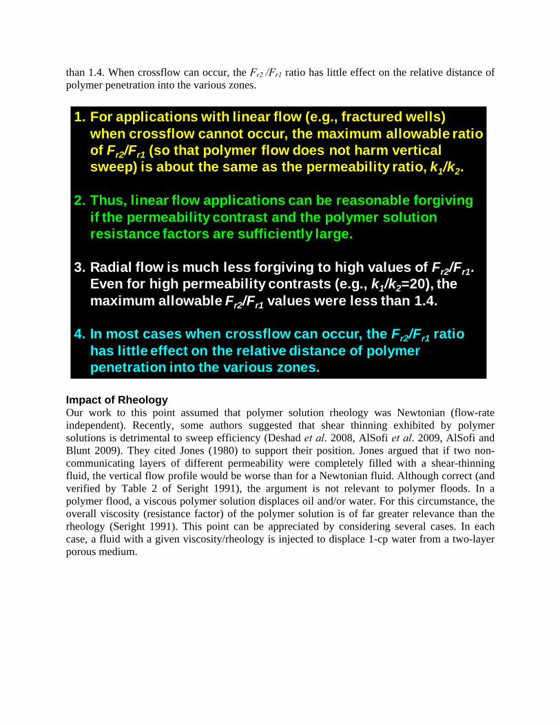
than 1.4. When crossflow can occur, the Fr2 /Fr1 ratio has little effect on the relative distance of polymer penetration into the various zones.

Impact of Rheology Our work to this point assumed that polymer solution rheology was Newtonian (flow-rate independent). Recently, some authors suggested that shear thinning exhibited by polymer solutions is detrimental to sweep efficiency (Deshad et al. 2008, AlSofi et al. 2009, AlSofi and Blunt 2009). They cited Jones (1980) to support their position. Jones argued that if two non-communicating layers of different permeability were completely filled with a shear-thinning fluid, the vertical flow profile would be worse than for a Newtonian fluid. Although correct (and verified by Table 2 of Seright 1991), the argument is not relevant to polymer floods. In a polymer flood, a viscous polymer solution displaces oil and/or water. For this circumstance, the overall viscosity (resistance factor) of the polymer solution is of far greater relevance than the rheology (Seright 1991). This point can be appreciated by considering several cases. In each case, a fluid with a given viscosity/rheology is injected to displace 1-cp water from a two-layer porous medium.

1. For applications with linear flow (e.g., fractured wells) when crossflow cannot occur, the maximum allowable ratio of Fr2/Fr1 (so that polymer flow does not harm vertical sweep) is about the same as the permeability ratio, k1/k2.

2. Thus, linear flow applications can be reasonable forgiving if the permeability contrast and the polymer solution resistance factors are sufficiently large.

3. Radial flow is much less forgiving to high values of Fr2/Fr1. Even for high permeability contrasts (e.g., k1/k2=20), the maximum allowable Fr2/Fr1 values were less than 1.4.

4. In most cases when crossflow can occur, the Fr2/Fr1 ratio has little effect on the relative distance of polymer penetration into the various zones.

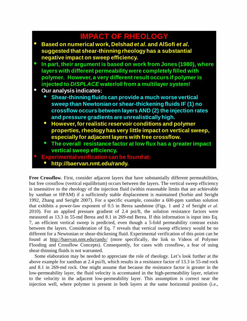
Free Crossflow. First, consider adjacent layers that have substantially different permeabilities, but free crossflow (vertical equilibrium) occurs between the layers. The vertical sweep efficiency is insensitive to the rheology of the injection fluid (within reasonable limits that are achievable by xanthan or HPAM) if a sufficiently stable displacement is maintained (Sorbie and Seright 1992, Zhang and Seright 2007). For a specific example, consider a 600-ppm xanthan solution that exhibits a power-law exponent of 0.5 in Berea sandstone (Figs. 1 and 2 of Seright et al. 2010). For an applied pressure gradient of 2.4 psi/ft, the solution resistance factors were measured as 13.3 in 55-md Berea and 8.1 in 269-md Berea. If this information is input into Eq. 7, an efficient vertical sweep is predicted, even though a 5-fold permeability contrast exists between the layers. Consideration of Eq. 7 reveals that vertical sweep efficiency would be no different for a Newtonian or shear-thickening fluid. Experimental verification of this point can be found at http://baervan.nmt.edu/randy/ (more specifically, the link to Videos of Polymer Flooding and Crossflow Concepts). Consequently, for cases with crossflow, a fear of using shear-thinning fluids is not warranted.

Some elaboration may be needed to appreciate the role of rheology. Let’s look further at the above example for xanthan at 2.4 psi/ft, which results in a resistance factor of 13.3 in 55-md rock and 8.1 in 269-md rock. One might assume that because the resistance factor is greater in the low-permeability layer, the fluid velocity is accentuated in the high-permeability layer, relative to the velocity in the adjacent low-permeability layer. This assumption is correct near the injection well, where polymer is present in both layers at the same horizontal position (i.e.,

IMPACT OF RHEOLOGY• Based on numerical work, Delshad et al. and AlSofi et al.

suggested that shear-thinning rheology has a substantial negative impact on sweep efficiency.

• In part, their argument is based on work from Jones (1980), where layers with different permeability were completely filled with polymer. However, a very different result occurs if polymer is injected to DISPLACE water/oil from a multilayer system!

• Our analysis indicates: • Shear-thinning fluids can provide a much worse vertical

sweep than Newtonian or shear-thickening fluids IF (1) no crossflow occurs between layers AND (2) the injection rates and pressure gradients are unrealistically high.

• However, for realistic reservoir conditions and polymer properties, rheology has very little impact on vertical sweep, especially for adjacent layers with free crossflow.

• The overall resistance factor at low flux has a greater impact vertical sweep efficiency.

• Experimental verification can be found at:• http://baervan.nmt.edu/randy.

where both Zones 1 and 2 are shaded gray in Fig. 13). In our example, near the injection well, the polymer solution is moving 8 times faster in the high-permeability layer than in the low-permeability layer [(i.e., (269/55)x(13.3/8.1)]. If only brine was present (i.e., before polymer injection), brine travels 4.9 times faster in the high-permeability layer than the low-permeability layer (i.e., 269/55). Thus, if a flow profile is measured at the injection wellbore (or at most horizontal locations where polymer is present in both layers), the shear-thinning xanthan solution appears to harm vertical sweep efficiency. However, this perception is incorrect. To appreciate why, focus on what happens just downstream of the polymer front in Zone 2 (the low-permeability layer in Fig. 13). Because of vertical equilibrium, the pressure gradient at that horizontal position is the same in both layers. The fluid at this horizontal position is water (with a resistance factor of 1) in Zone 2 and is polymer solution (with a resistance factor of 8.1) in Zone 1. The Darcy equations in Fig. 13 help to estimate the horizontal fluid velocities in the two layers at that position. Inputting the permeability and resistance factor values [(269/55)x(1/8.1)] yields a value of 0.6—suggesting that the front velocity in the low-permeability layer actually has the potential to travel faster than fluid in the high-permeability layer. Of course, this is not physically possible, because the pressure gradients involved would equalize the flow so that the velocity in the low-permeability layer never exceeds that in the high-permeability layer. But the analysis emphasizes that the polymer front in the low-permeability layer can travel at the same rate as the front in the high-permeability layer. To accomplish this, polymer from the high-permeability layer crossflows into the low-permeability layer in the vicinity of the polymer front. The relative fluid velocities upstream of the polymer front (e.g., near the injection well) are largely irrelevant. This leaves us with the ironic situation that flow profiles taken at the injection well incorrectly suggest that a shear-thinning fluid has harmed vertical sweep efficiency, whereas in reality, the vertical sweep is as good as it can possibly be (i.e., the same front velocity in both layers). One can experiment with the equations associated with Fig. 13 to appreciate that rheology has a less important effect on vertical sweep efficiency than the overall viscosity level of the polymer solution. For example, using resistance factors of 13.3 in the high-permeability zone and 8.1 in the low-permeability zone (i.e., shear-thickening behavior) results in the polymer fronts moving at the same rate in both layers—just as it did with shear-thinning behavior. In contrast, if the resistance factors have a value of two in both layers, the polymer front in the low-permeability zone only moves at 41% of the rate in the high-permeability zone (i.e., 2x55/269). No Crossflow, Radial Flow. Next, consider layers or pathways that are distinctly separated (i.e., no crossflow between layers). For two non-communicating layers with a 10-fold permeability contrast, the central part of Table 4 (calculations taken from Seright 1991) shows the relative differences for the displacement (polymer) fronts with radial flow of various rheologies and for factors up to a 100-fold difference in applied pressure drop between the well and the outer drainage radius. In Table 4, four Newtonian cases are listed. Fr=1 means that the injected fluid has the same viscosity as the water that is being displaced. Fr=1,000 means that the injected fluid is 1,000 times more viscous than the water that is being displaced. The low-viscosity shear-thinning fluid in Table 4 was based on a 200-ppm xanthan solution and a Carreau model that had a zero-shear resistance factor of 2.25, a power-law exponent of 0.88, and a second-Newtonian-region resistance factor of 1.1. The high-viscosity shear-thinning fluid was based on a 2,400-ppm xanthan solution and a Carreau model that had a zero-shear resistance factor of 182, a power-law exponent of 0.36, and a second-Newtonian-region resistance factor of 1.5 (from Fig. 2 of Seright 1991). The low-viscosity shear-thickening fluid in Table 4 was based on a 1-million-dalton

HPAM and a Heemskerk model (Heemskerk 1984) that provided resistance factors of ~7 at low flux and 20 at 1,000 ft/d. The high-viscosity shear-thickening fluid was based on a 26-million-dalton HPAM and a Heemskerk model that provided resistance factors of ~100 at low flux and 1,000 at 100 ft/d (Fig. 3 of Seright 1991).

For very high pressure drops in Table 4 (i.e., 5,000 psi over 50 ft), the high-viscosity shear-thickening model indicated a flow profile that was 17% more favorable than for a 100-cp Newtonian fluid (0.417 versus 0.357), which in turn, was 10% more favorable than for the high-viscosity shear-thinning fluid (0.357 versus 0.325). These differences were not particularly large and they diminished when lower, more-realistic pressure drops were applied. For a pressure drop of 50 psi over 50 ft (first data column of Table 4), only a 1.5% difference separated the high-viscosity shear-thickening fluid from the high-viscosity shear-thinning fluid (0.344 versus 0.339).

Table 4—Distance of polymer penetration into a 100-md layer relative to that in a 1,000-md layer (no crossflow)

Data from Seright 1991 Radial flow Linear flow

(rp2-rw)/(rp1-rw) Lp2/Lp1

Pressure drop (psi over 50 ft for radial flow) or pressure gradient (psi/ft, for linear flow):

50 500 5000 1 10 100 1000

Assumed rheology: Newtonian, Fr=1 0.309 0.309 0.309 0.100 0.100 0.100 0.100 Newtonian, Fr=10 0.352 0.352 0.352 0.256 0.256 0.256 0.256 Newtonian, Fr=100 0.357 0.357 0.357 0.309 0.309 0.309 0.309 Newtonian, Fr=1,000 0.358 0.358 0.358 0.316 0.316 0.316 0.316 Low-viscosity, shear-thinning, Xanthan, Carreau model 0.329 0.326 0.324 0.145 0.136 0.129 0.123 High-viscosity,shear-thinning, Xanthan, Carreau model 0.339 0.326 0.325 0.312 0.295 0.172 0.131 Low-viscosity, shear-thickening, HPAM, Heemskerk model 0.343 0.365 0.379 0.201 0.194 0.236 0.274 High-viscosity, shear-thickening, HPAM, Heemskerk model 0.344 0.410 0.417 0.299 0.300 0.311 0.315

No Crossflow, Linear Flow. Most polymer floods to date may have had open fractures intersecting the injection wells (Seright et al. 2009c). Therefore, linear flow cases may be the most relevant. In the right part of Table 4 (the cases for linear flow with no vertical communication between layers), there are large percentage differences in the vertical flow profiles for different rheologies. For some cases at high pressure gradients, the shear-thinning fluid gave a noticeably less efficient displacement than for the Newtonian or shear-thickening fluids. However, the differences were most pronounced at high pressure gradients that are unlikely to be achieved in real field applications (>10 psi/ft). For relatively low-pressure gradients, the high-viscosity shear-thinning fluid gave a vertical sweep no worse than the Newtonian or shear-thickening fluids. In summary, for practical conditions during polymer floods, the vertical sweep efficiency using shear-thinning fluids is not expected to be dramatically different from that for Newtonian or shear-thickening fluids. As mentioned earlier, the overall viscosity (resistance factor) of the polymer solution is of far greater relevance than the rheology. Fractional Flow Calculations for Polymer Flooding After Waterflooding. One Homogeneous Layer. In our previous work (Seright 2010), we used fractional flow calculations to examine the potential of polymer flooding when the polymer flood was initiated immediately after primary recovery—i.e., with no intermediate water flood. In this section, we

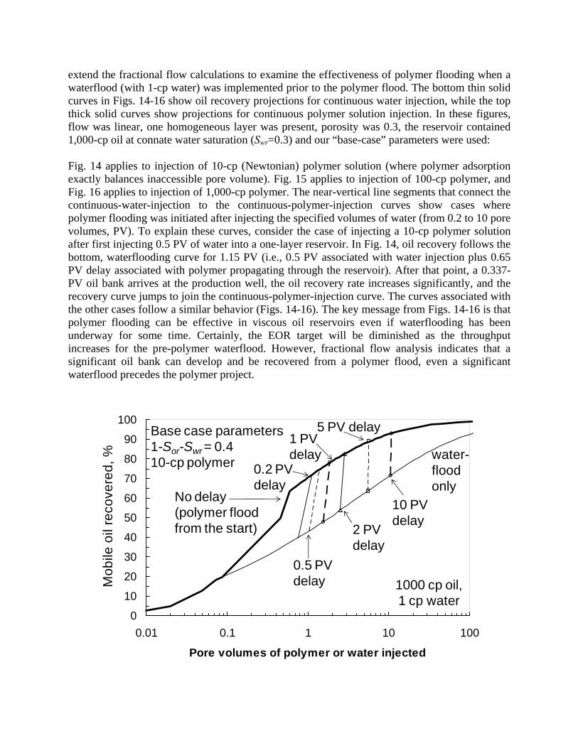
extend the fractional flow calculations to examine the effectiveness of polymer flooding when a waterflood (with 1-cp water) was implemented prior to the polymer flood. The bottom thin solid curves in Figs. 14-16 show oil recovery projections for continuous water injection, while the top thick solid curves show projections for continuous polymer solution injection. In these figures, flow was linear, one homogeneous layer was present, porosity was 0.3, the reservoir contained 1,000-cp oil at connate water saturation (Swr=0.3) and our “base-case” parameters were used: Fig. 14 applies to injection of 10-cp (Newtonian) polymer solution (where polymer adsorption exactly balances inaccessible pore volume). Fig. 15 applies to injection of 100-cp polymer, and Fig. 16 applies to injection of 1,000-cp polymer. The near-vertical line segments that connect the continuous-water-injection to the continuous-polymer-injection curves show cases where polymer flooding was initiated after injecting the specified volumes of water (from 0.2 to 10 pore volumes, PV). To explain these curves, consider the case of injecting a 10-cp polymer solution after first injecting 0.5 PV of water into a one-layer reservoir. In Fig. 14, oil recovery follows the bottom, waterflooding curve for 1.15 PV (i.e., 0.5 PV associated with water injection plus 0.65 PV delay associated with polymer propagating through the reservoir). After that point, a 0.337-PV oil bank arrives at the production well, the oil recovery rate increases significantly, and the recovery curve jumps to join the continuous-polymer-injection curve. The curves associated with the other cases follow a similar behavior (Figs. 14-16). The key message from Figs. 14-16 is that polymer flooding can be effective in viscous oil reservoirs even if waterflooding has been underway for some time. Certainly, the EOR target will be diminished as the throughput increases for the pre-polymer waterflood. However, fractional flow analysis indicates that a significant oil bank can develop and be recovered from a polymer flood, even a significant waterflood precedes the polymer project.

0

10

20

30

40

50

60

70

80

90

100

0.01 0.1 1 10 100


Mo

bile

oil

reco

vere

d,

%

No delay(polymer flood from the start)


Base case parameters1-Sor-Swr = 0.410-cp polymer

0.5 PV delay

1 PVdelay

2 PVdelay

5 PV delay

10 PVdelay

water-flood only

0.2 PV delay

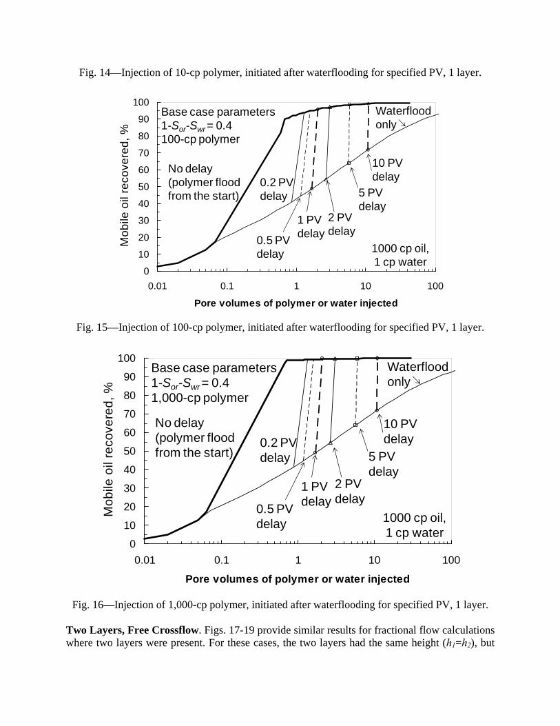
Fig. 14—Injection of 10-cp polymer, initiated after waterflooding for specified PV, 1 layer.

Fig. 15—Injection of 100-cp polymer, initiated after waterflooding for specified PV, 1 layer.

Fig. 16—Injection of 1,000-cp polymer, initiated after waterflooding for specified PV, 1 layer.

Two Layers, Free Crossflow. Figs. 17-19 provide similar results for fractional flow calculations where two layers were present. For these cases, the two layers had the same height (h1=h2), but

0

10

20

30

40

50

60

70

80

90

100

0.01 0.1 1 10 100


Mo

bile

oil

reco

vere

d,

%


0.5 PVdelay

1 PVdelay

2 PVdelay

5 PVdelay

Waterflood only


10 PVdelay

Base case parameters1-Sor-Swr = 0.4100-cp polymer

0.2 PVdelay

0

10

20

30

40

50

60

70

80

90

100

0.01 0.1 1 10 100


Mo

bile

oil

reco

vere

d,

%


0.5 PVdelay

1 PVdelay

2 PVdelay

5 PVdelay

Waterflood only


10 PVdelay

Base case parameters1-Sor-Swr = 0.41,000-cp polymer

0.2 PVdelay

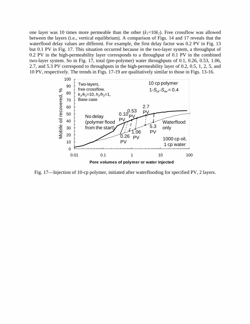
one layer was 10 times more permeable than the other (k1=10k2). Free crossflow was allowed between the layers (i.e., vertical equilibrium). A comparison of Figs. 14 and 17 reveals that the waterflood delay values are different. For example, the first delay factor was 0.2 PV in Fig. 13 but 0.1 PV in Fig. 17. This situation occurred because in the two-layer system, a throughput of 0.2 PV in the high-permeability layer corresponds to a throughput of 0.1 PV in the combined two-layer system. So in Fig. 17, total (pre-polymer) water throughputs of 0.1, 0.26, 0.53, 1.06, 2.7, and 5.3 PV correspond to throughputs in the high-permeability layer of 0.2, 0.5, 1, 2, 5, and 10 PV, respectively. The trends in Figs. 17-19 are qualitatively similar to those in Figs. 13-16.

Fig. 17—Injection of 10-cp polymer, initiated after waterflooding for specified PV, 2 layers.

0

10

20

30

40

50

60

70

80

90

100

0.01 0.1 1 10 100


Mo

bile

oil

reco

vere

d,

%

10 cp polymer


1-Sor-Swr = 0.4Two-layers, free crossflow, k1/k2=10, h1/h2=1,Base case

0.26 PV

0.53 PV

1.06 PV

2.7 PV

5.3 PV

Waterflood only


0.10 PV

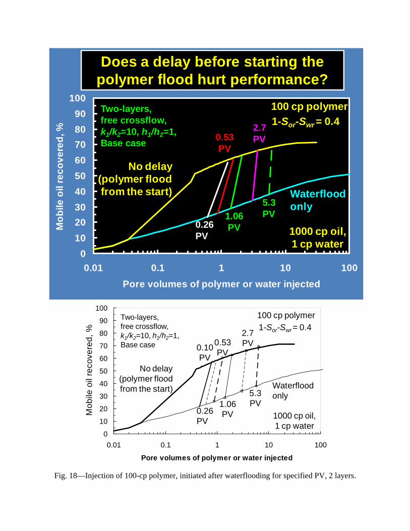
Fig. 18—Injection of 100-cp polymer, initiated after waterflooding for specified PV, 2 layers.

0

10

20

30

40

50

60

70

80

90

100

0.01 0.1 1 10 100


Mo

bile

oil

rec

ov

ere

d, %

100 cp polymer


Does a delay before starting the polymer flood hurt performance?


0.26 PV

0.53 PV

1.06 PV

2.7 PV

5.3 PV

Waterflood only


0

10

20

30

40

50

60

70

80

90

100

0.01 0.1 1 10 100


Mo

bile

oil

reco

vere

d,

%

100 cp polymer



0.26 PV

0.53 PV

1.06 PV

2.7 PV

5.3 PV

Waterflood only


0.10 PV

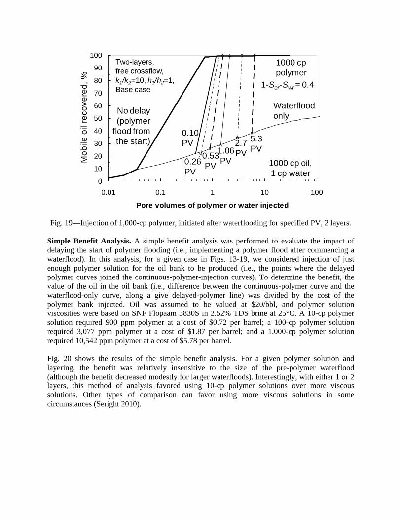
Fig. 19—Injection of 1,000-cp polymer, initiated after waterflooding for specified PV, 2 layers.

Simple Benefit Analysis. A simple benefit analysis was performed to evaluate the impact of delaying the start of polymer flooding (i.e., implementing a polymer flood after commencing a waterflood). In this analysis, for a given case in Figs. 13-19, we considered injection of just enough polymer solution for the oil bank to be produced (i.e., the points where the delayed polymer curves joined the continuous-polymer-injection curves). To determine the benefit, the value of the oil in the oil bank (i.e., difference between the continuous-polymer curve and the waterflood-only curve, along a give delayed-polymer line) was divided by the cost of the polymer bank injected. Oil was assumed to be valued at $20/bbl, and polymer solution viscosities were based on SNF Flopaam 3830S in 2.52% TDS brine at 25°C. A 10-cp polymer solution required 900 ppm polymer at a cost of $0.72 per barrel; a 100-cp polymer solution required 3,077 ppm polymer at a cost of $1.87 per barrel; and a 1,000-cp polymer solution required 10,542 ppm polymer at a cost of $5.78 per barrel. Fig. 20 shows the results of the simple benefit analysis. For a given polymer solution and layering, the benefit was relatively insensitive to the size of the pre-polymer waterflood (although the benefit decreased modestly for larger waterfloods). Interestingly, with either 1 or 2 layers, this method of analysis favored using 10-cp polymer solutions over more viscous solutions. Other types of comparison can favor using more viscous solutions in some circumstances (Seright 2010).

0

10

20

30

40

50

60

70

80

90

100

0.01 0.1 1 10 100


Mo

bile

oil

reco

vere

d,

%

1000 cppolymer


1-Sor-Swr = 0.4

Two-layers, free crossflow, k1/k2=10, h1/h2=1,Base case

0.26 PV

0.53 PV

1.06 PV

2.7 PV

5.3 PV

Waterflood only

No delay(polymer

flood fromthe start)

0.10 PV

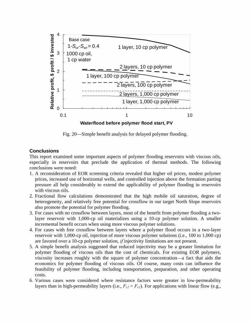
Fig. 20—Simple benefit analysis for delayed polymer flooding.

Conclusions This report examined some important aspects of polymer flooding reservoirs with viscous oils, especially in reservoirs that preclude the application of thermal methods. The following conclusions were noted: 1. A reconsideration of EOR screening criteria revealed that higher oil prices, modest polymer

prices, increased use of horizontal wells, and controlled injection above the formation parting pressure all help considerably to extend the applicability of polymer flooding in reservoirs with viscous oils.

2. Fractional flow calculations demonstrated that the high mobile oil saturation, degree of heterogeneity, and relatively free potential for crossflow in our target North Slope reservoirs also promote the potential for polymer flooding.

3. For cases with no crossflow between layers, most of the benefit from polymer flooding a two-layer reservoir with 1,000-cp oil materializes using a 10-cp polymer solution. A smaller incremental benefit occurs when using more viscous polymer solutions.

4. For cases with free crossflow between layers where a polymer flood occurs in a two-layer reservoir with 1,000-cp oil, injection of more viscous polymer solutions (i.e., 100 to 1,000 cp) are favored over a 10-cp polymer solution, if injectivity limitations are not present.

5. A simple benefit analysis suggested that reduced injectivity may be a greater limitation for polymer flooding of viscous oils than the cost of chemicals. For existing EOR polymers, viscosity increases roughly with the square of polymer concentration—a fact that aids the economics for polymer flooding of viscous oils. Of course, many costs can influence the feasibility of polymer flooding, including transportation, preparation, and other operating costs.

6. Various cases were considered where resistance factors were greater in low-permeability layers than in high-permeability layers (i.e., Fr2 > Fr1). For applications with linear flow (e.g.,

0

1

2

3

4

0.1 1 10

Waterflood before polymer flood start, PV

Re

lati

ve

pro

fit,

$ p

rofi

t / $

inv

es

ted

1 layer, 10 cp polymer1000 cp oil, 1 cp water

1-Sor-Swr = 0.4Base case

2 layers, 10 cp polymer

2 layers, 100 cp polymer

2 layers, 1,000 cp polymer

1 layer, 1,000 cp polymer

1 layer, 100 cp polymer

fractured wells) with no crossflow, the maximum allowable ratio of Fr2 /Fr1 (so that polymer injection does not harm vertical sweep) is about the same as the permeability ratio, k1 /k2. Thus, linear flow applications can be reasonably forgiving if the permeability contrast and the polymer solution resistance factors are sufficiently large. Radial flow (with no crossflow) is much less forgiving to high Fr2 /Fr1 values. Even for high-permeability contrasts (e.g., k1 /k2 = 20), the maximum allowable Fr2 /Fr1 values were less than 1.4. When crossflow can occur, the Fr2 /Fr1 ratio has little effect on the relative distance of polymer penetration into the various zones.

7. For practical conditions during polymer floods, the vertical sweep efficiency using shear-thinning fluids is not expected to be dramatically different from that for Newtonian or shear-thickening fluids. The overall viscosity (resistance factor) of the polymer solution is of far greater relevance than the rheology.

8. We extended the fractional flow calculations to examine the effectiveness of polymer flooding when a waterflood (with 1-cp water) was implemented prior to the polymer flood. We showed that polymer flooding can be effective in viscous (1,000-cp) oil reservoirs even if waterflooding has been underway for some time. Certainly, the EOR target will be diminished as the throughput increases for the pre-polymer waterflood. However, fractional flow analysis indicates that a significant oil bank can develop and be recovered from a polymer flood, even if a significant waterflood precedes the polymer project. This point was demonstrated both with a homogeneous 1-layer reservoir and in a 2-layer reservoir with free crossflow.

Nomenclature C = polymer concentration, ppm [g/cm3] Fr = resistance factor (water mobility/polymer solution mobility) Frr = residual resistance factor (water mobility before polymer/water mobility after polymer) Fr1 = resistance factor in Layer 1(high-permeability layer) Fr2 = resistance factor in Layer 2 (low-permeability layer) h = formation height, ft [m] h1 = height of Zone 1, ft [m] h2 = height of Zone 2, ft [m] k = permeability, darcys [m2] kro = relative permeability to oil kroo = endpoint relative permeability to oil krw = relative permeability to water krwo = endpoint relative permeability to water k1 = permeability of Zone 1, darcys [m2] k2 = permeability of Zone 2, darcys [m2] L = linear distance, ft [m] Lp1 = linear distance of polymer penetration into the high-permeability layer, ft [m] Lp2 = linear distance of polymer penetration into the low-permeability layer, ft [m] no = oil saturation exponent in Eq. 2 nw = water saturation exponent in Eq. 1 PV = pore volumes of fluid injected p = pressure difference, psi [Pa] rp1 = radius of polymer penetration into the high-permeability layer, ft [m] rp2 = radius of polymer penetration into the low-permeability layer, ft [m]

rw = wellbore radius, ft [m] Sor = residual oil saturation Sw = water saturation Swr = residual water saturation u = flux, ft/d [m/d] v1 = front velocity in Zone 1, ft/d [m/d] v2 = front velocity in Zone 2, ft/d [m/d] = mobility, darcys/cp [m2/ mPa-s] = viscosity, cp [mPa-s] = porosity 1 = porosity in Zone 1 2 = porosity in Zone 2 = density difference, g/cm3 References AlSofi, A. M., LaForce, T.C., and Blunt, M.J. 2009. Sweep Impairment Due to Polymers Shear

Thinning. Paper SPE 120321 presented at the SPE Middle East Oil & Gas Show and Conference, Bahrain, Louisiana, 15-18 March.

AlSofi, A. M., and Blunt, M.J. 2009. Streamline-Based Simulation of Non-Newtonian Polymer Flooding. Paper SPE 123971 presented at the SPE Annual Technical Conference and Exhibition, New Orleans, Louisiana, 4–7 October.

Beliveau, D. 2009. Waterflooding Viscous Oil Reservoirs. SPEREE 12 (5): 689–701. Buchgraber, M., Clements, T., Castanier, L.M., and Kovseck, A.R. 2009. The Displacement of Viscous Oil by Associative Polymer Solutions, Paper SPE 122400 presented at the SPE Annual Technical Conference and Exhibition, New Orleans, Louisiana, 4–7 October. Cannella, W.J., Huh, C., and Seright, R.S. 1988. Prediction of Xanthan Rheology in Porous

Media. Paper SPE 18089 presented at the SPE Annual Technical Conference and Exhibition, Houston, Texas, 2–5 October.

Chauveteau, G. 1982. Rodlike Polymer Solution Flow through Fine Pores: Influence of Pore Size on Rheological Behavior. J. Rheology 26 (2): 111–142.

Coats, K.H., Dempsey, J.R., and Henderson, J.H. 1971. The Use of Vertical Equilibrium in Two-Dimensional Simulation of Three-Dimensional Reservoir Performance. SPEJ, 11(1): 63–71.

Craig, F.F. 1971. The Reservoir Engineering Aspects of Waterflooding. Monograph Series, SPE, Richardson, Texas 3: 45–75.

Dawson, R., and Lantz, R.B. 1972. Inaccessible Pore Volume in Polymer Flooding. SPEJ 12 (5): 448–452.

Delshad, M., Kim, D.H., Magbagbeolz, O.A., Huh, C., Pope, G.A., and Tarahhom, F. 2008. Mechanistic Interpretation and Utilization of Viscoselastic Behavior of Polymer Solutions for Improved Polymer-Flood Efficiency. Paper SPE 113620 presented at the SPE/DOE Improved Oil Recovery Symposium, Tulsa, Oklahoma, 19–23 April.

Green, D.W., and Willite, G.P. 1998. Enhanced Oil Recovery. Textbook Series, SPE, Richardson, Texas 6: 100–185.

Heemskerk, J., Rosmalen, R.J., Hotslag, R.J., and Teeuw, D. 1984. Quantification of Viscoelastic Effects of Polyacrylamide Solutions. Paper SPE 12652 presented at the SPE/DOE Symposium on Enhanced Oil Recovery Symposium, Tulsa, Oklahoma, 15–18 April.

Hirasaki, G.J., and Pope, G.A. 1974. Analysis of Factors Influencing Mobility and Adsorption in the Flow of Polymer Solution Through Porous Media. SPEJ 14 (4): 337–346.

Huh, C., and Pope, G.A. 2008. Residual Oil Saturation from Polymer Floods: Laboratory Measurements and Theoretical Interpretation. Paper SPE 113417 presented at the SPE/DOE Improved Oil Recovery Symposium, Tulsa, Oklahoma, 19–23 April.

Jennings, R.R., Rogers, J.H., and West, T.J. 1971. Factors Influencing Mobility Control by Polymer Solutions. JPT 23(3): 391–50, SPE 2867-PA.

Jewett, R.L. and Schurz G.F. 1979 Polymer Flooding—A Current Appraisal. JPT 31(6): 675–684.

Jones, W.M. 1980. Polymer Additives for Reservoir Flooding for Oil Recovery: Shear Thinning or Shear Thickening? J. Phy. D.: Appl. Phys. 13: L87-88.

Khodaverdian, M., Sorop, T. Postif, S. and Van den Hoek, P. 2009. Polymer Flooding in Unconsolidated Sand Formations: Fracturing and Geomechnanical Considerations. Paper SPE121840 presented at the SPE EUROPEC/EAGE Annual Conference and Exhibition in Amsterdam, The Netherlands, 8-11 June.

Kumar, M., Hoang, V., Satik, C., and Rojas, D. 2008. High-Mobility-Ratio-Waterflood Performance Prediction: Challenges and New Insights, SPEREE 11 (1): 186–196.

Lake, L.W. 1989. Enhanced Oil Recovery. 314–353, Englewood Cliffs, New Jersey: Prentice Hall, Inc.

Lee, S., Kim, D.H., Huh, C., and Pope, G.A. 2009. Development of a Comprehensive Rheological Property Database for EOR Polymers. Paper SPE 124798 presented at the SPE Annual Technical Conference and Exhibition, New Orleans, Louisiana, 4–7 October.

Liang, J., Lee, R.L., and Seright, R.S. 1993. Placement of Gels in Production Wells. SPEPF 8 (1): 276–284; Transactions AIME 295.

Maitin, B.K. 1992. Performance Analysis of Several Polyacrylamide Floods in North German Oil Fields. Paper SPE 24118 presented at the SPE/DOE Symposium on Improved Oil Recovery, Tulsa, Oklahoma, 22–24 April.

Manning, R.K., Pope, G.A., Lake, L.W., and Paul, G.W. 1983. A Technical Survey of Polymer Flooding Projects. Report, Contract No. DOE/BC10327-19, US DOE, Washington, DC (September 1983).

Morel, D., Vert, M., Jouenne, S., and Nahas, E. 2008. Polymer Injection in Deep Offshore Field: The Dalia Angola Case. Paper 116672 presented at the SPE Annual Technical Conference and Exhibition, Denver, Colorado, 21–24 September.

Pye, D.J. 1964. Improved Secondary Recovery by Control of Water Mobility. JPT 16(8): 911–916, SPE 845-PA.

Rousseau, D., Chauveteau, G. and Renard, M. 2005. Rheology and Transport in Porous Media of New Water Shutoff/Conformance Control Microgels. Paper SPE 93254 presented at the SPE International Symposium on Oilfield Chemistry, Houston, Texas, 2–4 February.

Seright, R.S. 1983. The Effects of Mechanical Degradation and Viscoelastic Behavior on Injectivity of Polyacrylamide Solutions. SPEJ 23 (3): 475–485, SPE 9297-PA.

Seright, R.S. 1988. Placement of Gels to Modify Injection Profiles. Paper SPE/DOE 17332 presented at the SPE/DOE Enhanced Oil Recovery Symposium, Tulsa, Oklahoma, 17–20 April.

Seright, R.S. 1991. Effect of Rheology on Gel Placement. SPERE 6 (2): 212–218; Trans., AIME, 291.

Seright, R.S. 1993. Improved Techniques for Fluid Diversion in Oil Recovery. First Annual

Report. Contract No. DE94000113. U.S. Department of Energy, Washington, DC (December 1993): 2–72.

Seright, R.S., and Liang, J-T. 1994. A Survey of Field Applications of Gel Treatments for Water Shutoff. Paper SPE 26991 presented at the SPE Latin American and Caribbean Petroleum Engineering Conference, Buenos Aires, Argentina, 27–29 April.

Seright, R.S. 2009a. http://baervan.nmt.edu/randy/. Seright, R.S. 2009b. Use of Polymers to Recover Viscous Oil from Unconventional Reservoirs.

First Annual Report, U.S. Department of Energy, DOE Contract No.: DE-NT0006555, US DOE, Washington, DC (October 2009).

Seright, R.S., Seheult, J.M., and Talashek, T.A. 2009c. Injectivity Characteristics of EOR Polymers. SPEREE (October): 783-792.

Seright, R.S., Fan, T., Wavrik, K., and Balaban, R.C. 2010. New Insights into Polymer Rheology in Porous Media. Paper SPE 129200 presented at the SPE Improved Oil Recovery Symposium, Tulsa, Oklahoma, USA, 24–28 April.

Smith, F.W. 1970. The Behavior of Partially Hydrolyzed Polyacrylamide Solutions in Porous Media. JPT 22(2): 148–156. SPE 2422-PA. Sorbie, K.S. 1991. Polymer-Improved Oil Recovery. 115. Glasgow, Scotland: Blackie and Son,

Ltd. Sorbie, K.S. and Seright, R.S. 1992. Gel Placement in Heterogeneous Systems with Crossflow.

Paper SPE 24192 presented at the SPE/DOE Symposium on Enhanced Oil Recovery, Tulsa, Oklahoma, 22–24 April.

Stryker, A.R., Watkins, R., Olsen, D.K., et al. 1995. Feasibility Study of Heavy Oil Recovery in the United States. Final Report, Contract No. DE-AC2294PC91008, US DOE, Washington, DC (September 1995).

Taber, J.J. and Seright, R.S. 1992. Horizontal Injection and Production Wells for EOR. Paper SPE 23952 presented at the SPE/DOE Symposium on Enhanced Oil Recovery, Tulsa, Oklahoma, 22–24 April.

Taber, J.J., Martin, F.D., and Seright, R.S. 1997a. EOR Screening Criteria Revisited - Part 1, Introduction to Screening Criteria and Enhanced Recovery Field Projects. SPERE 12 (3): 189–198.

Taber, J.J., Martin, F.D., and Seright, R.S. 1997b. EOR Screening Criteria Revisited - Part 2: Applications and Impact of Oil Prices. SPERE 12 (3): 199–205.

Thomas, C.P., Faulder, D.D., Doughty, T.C., Hite, D.M., and White, G.J. 2007. Alaska North Slope Oil and Gas, a Promising Future or an Area in Decline? Summary Report DOE/NETL-2007/1279, US DOE, Washington, DC (August 2007)

Trantham, J.C., Threlkeld, C.B., and Patterson, H.L. 1980. Reservoir Description for a Surfactant/Polymer Pilot in a Fractured, Oil-Wet Reservoir—North Burbank Unit Tract 97. JPT 32 (9): 1647–1656.

Van den Hoek, P.J., Al-Masfry, R., Zwarts, D., Jansen, J.D., Hustedt, B., and van Schijndel, L. 2009. Optimizing Recovery for Waterflooding under Dynamic Induced Fracturing Conditions. SPEREE 12 (5): 671–682.

Vela, S., Peaceman, D.W. and Sandvik, E.I. 1976. Evaluation of Polymer Flooding in a Layered Reservoir with Crossflow, Retention, and Degradation. SPEJ 16(2): 82–96.

Wang, D., Zhang, J., Meng, F., et al. 1995. Commercial Test of Polymer Flooding in Daqing Oil Field. Paper SPE 29902 presented at the SPE International Meeting on Petroleum Engineering, Beijing, China, 14–17 November.

Wang, D.M., Han, P., Shao, Z., Weihong, H., and Seright, R.S. 2008a. Sweep Improvement Options for the Daqing Oil Field. SPEREE 11 (1):18–26. SPE-994441-PA. doi: 10.2118/9944-PA.

Wang, D.M., Seright, R.S., Shao, Z., and Wang, J. 2008b. Key Aspects of Project Design for Polymer Flooding at the Daqing Oil Field. SPEREE 11 (6): 1117–1124.

Wang, D.M., Dong, H., Lv, C., Fu, X., and Nie, J. 2009. Review of Practical Experience of Polymer Flooding at Daqing. SPEREE 12 (3): 470–476.

Wu, W., Wang, D., and Jiang, H. 2007. Effect of the Visco-Elasiticity of Displacing Fluids on the Relationship of Capillary Number and Displacement Efficiency in Weak Oil-Wet Cores. Paper SPE 109228 presented at the SPE Asia Pacific Oil and Gas Conference and Exhibition, Jakarta, Indonesia, 30 October–1 November.

Zaitoun, A. and Kohler, N. 1987. The Role of Adsorption in Polymer Propagation Through Reservoir Rocks. Paper SPE 16274 presented at the SPE International Symposium on Oilfield Chemistry, San Antonio, Texas, 4–6 October.

Zapata, V.J. and Lake, L.W. 1981. A Theoretical Analysis of Viscous Crossflow. Paper SPE 10111 presented at the SPE Annual Technical Conference and Exhibition, San Antonio, Texas, 5–7 October.

Zhang, G. and Seright, R.S. 2007. Conformance and Mobility Control: Foams versus Polymers. Paper SPE 105907 presented at the SPE International Symposium on Oilfield Chemistry, Houston, Texas, 28 February–2 March.

Documents

Potential for Polymer Flooding Reservoirs with Viscous Oilsbaervan.nmt.edu/groups/res-sweep/media/pdf/Potential for Polymer... · when a waterflood (with 1-cp water) was implemented