Embed Size (px)
Citation preview

Post-tensioning of Reinforced Concrete Trough Bridge Decks – Laboratory test
Jonny Nilimaa
Department of Civil, Environmental and Natural resources engineering
Luleå University of Technology
SE-97187 Luleå, Sweden

i
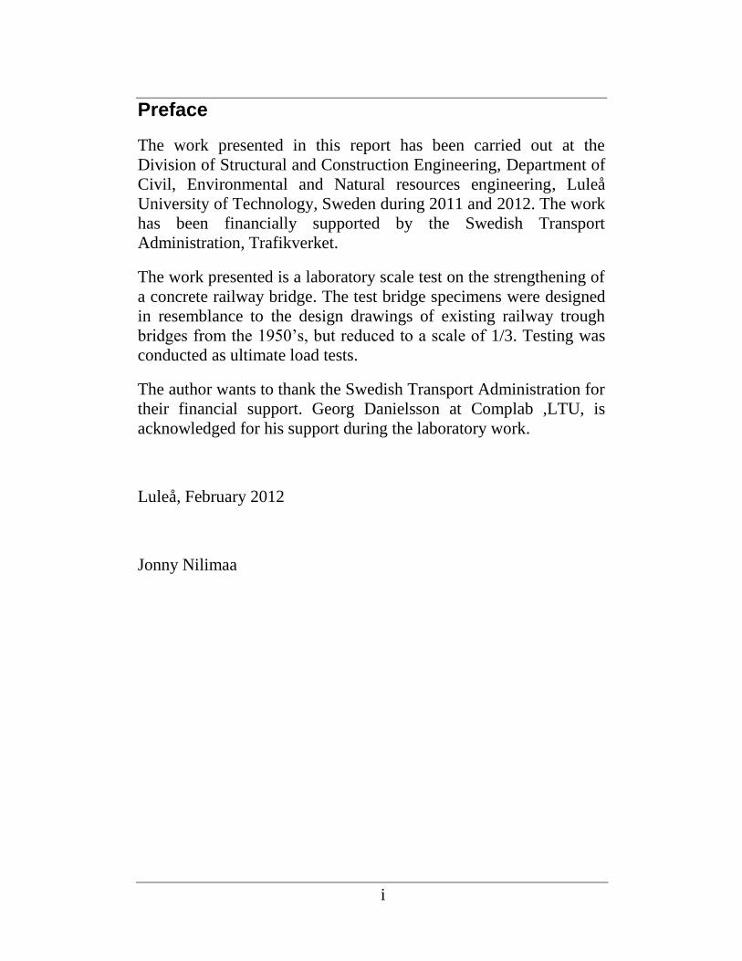
Preface
The work presented in this report has been carried out at the
Division of Structural and Construction Engineering, Department of
Civil, Environmental and Natural resources engineering, Luleå
University of Technology, Sweden during 2011 and 2012. The work
has been financially supported by the Swedish Transport
Administration, Trafikverket.
The work presented is a laboratory scale test on the strengthening of
a concrete railway bridge. The test bridge specimens were designed
in resemblance to the design drawings of existing railway trough
bridges from the 1950’s, but reduced to a scale of 1/3. Testing was
conducted as ultimate load tests.
The author wants to thank the Swedish Transport Administration for
their financial support. Georg Danielsson at Complab ,LTU, is
acknowledged for his support during the laboratory work.
Luleå, February 2012
Jonny Nilimaa

ii
iii
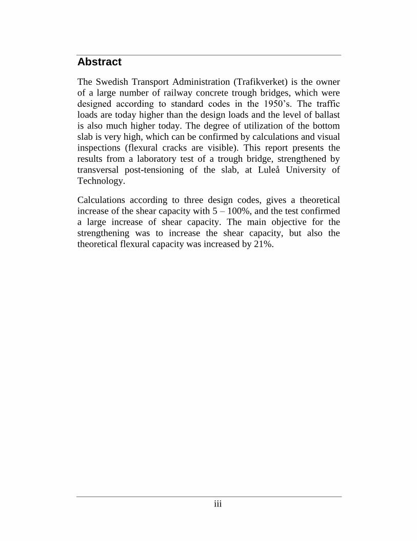
Abstract
The Swedish Transport Administration (Trafikverket) is the owner
of a large number of railway concrete trough bridges, which were
designed according to standard codes in the 1950’s. The traffic
loads are today higher than the design loads and the level of ballast
is also much higher today. The degree of utilization of the bottom
slab is very high, which can be confirmed by calculations and visual
inspections (flexural cracks are visible). This report presents the
results from a laboratory test of a trough bridge, strengthened by
transversal post-tensioning of the slab, at Luleå University of
Technology.
Calculations according to three design codes, gives a theoretical
increase of the shear capacity with 5 – 100%, and the test confirmed
a large increase of shear capacity. The main objective for the
strengthening was to increase the shear capacity, but also the
theoretical flexural capacity was increased by 21%.

iv

v
Table of content
PREFACE .................................................................................................................................... I
ABSTRACT .............................................................................................................................. III
1. BACKGROUND ................................................................................................................... 1
1.1. INTRODUCTION .......................................................................................................... 1 1.2. STRENGTHENING ........................................................................................................ 3
2. TEST SETUP......................................................................................................................... 4
2.1. LOADING AND MONITORING ....................................................................................... 5 2.2. TEST BRIDGE GEOMETRY ........................................................................................... 6 2.3. MATERIAL PROPERTIES .............................................................................................. 6 2.4. POST TENSIONING ...................................................................................................... 7
3. CALCULATIONS ................................................................................................................ 9
3.1. INTRODUCTORY EXAMPLE ......................................................................................... 9 3.2. SHEAR DESIGN ......................................................................................................... 12
3.2.1. Eurocode 2 ......................................................................................................... 13 3.2.2. CSA ..................................................................................................................... 14 3.2.3. BBK .................................................................................................................... 15
3.3. FLEXURAL DESIGN ................................................................................................... 17 3.4. CURVATURE............................................................................................................. 19
4. RESULTS ............................................................................................................................ 23
4.1. LOAD CURVES .......................................................................................................... 23 4.2. CRACK PATTERNS .................................................................................................... 27
5. ANALYSIS AND DISCUSSION ........................................................................................ 29
6. FUTURE RESEARCH ....................................................................................................... 31
7. REFERENCES ................................................................................................................... 33
APPENDIX A – DOCUMENTATION OF TEST PROCEDURE
APPENDIX B – TEST RESULTS
APPENDIX C – CALCULATIONS

vi
1
1. Background
1.1. Introduction
There are approximately 300,000 railway bridges in Europe and
about two thirds of them are more than 50 years old (Bell, 2004). As
the bridges get older, they not just start to deteriorate; the demands
on the performance are also changing. The society is constantly
evolving, forcing our infrastructure to change. The railway bridges
are affected by this evolvement by increases in traffic intensity,
loads, and velocities, as well as changed design criteria and design
codes. Eventually, all bridges will reach a point when they can no
longer provide a required safety margin for the users, i.e. it is no
longer safe to use the bridge in the present state.
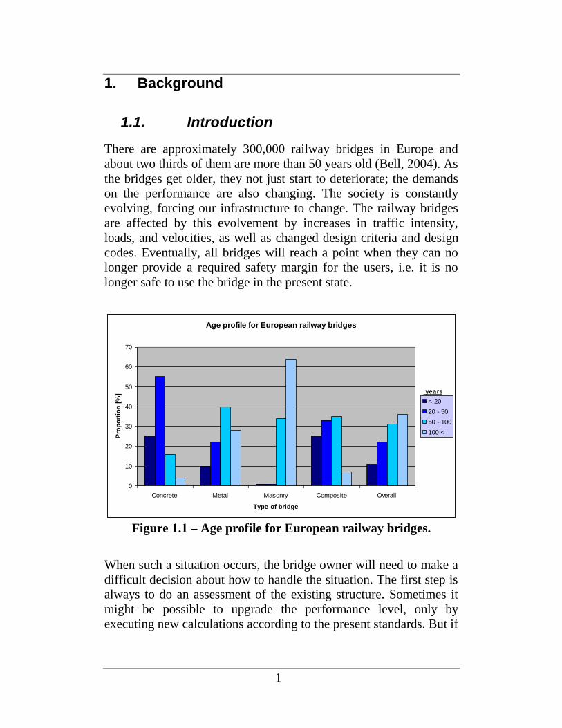
Age profile for European railway bridges
0
10
20
30
40
50
60
70
Concrete Metal Masonry Composite Overall
Type of bridge
Pro
po
rtio
n [
%]
< 20
20 - 50
50 - 100
100 <
years
Figure 1.1 – Age profile for European railway bridges.
When such a situation occurs, the bridge owner will need to make a
difficult decision about how to handle the situation. The first step is
always to do an assessment of the existing structure. Sometimes it
might be possible to upgrade the performance level, only by
executing new calculations according to the present standards. But if
2
the bridge can not be upgraded without any physical measures, there
are three possible alternatives for the bridge owner;
1) Keep using the existing structure, but with reduced capacity.
2) Strengthening of the existing structure, in order to increase
the capacity.
3) Replacing of the existing structure with a new that fulfils the
demands.
In some cases it might be possible to continue using the old
structure with a reduction in the capacity. But if the objective is to
e.g. increase the performance, this might not be a possible
alternative. There are many ways to strengthen a bridge and current
research is constantly developing new methods (e.g. Sas et.al,
2012), but it is not always economically or physically viable to
strengthen old structures.
The Swedish Transport Administration (Trafikverket) is the owner
of a large number of railway concrete trough bridges, which were
designed according to standard codes in the 1950’s. The traffic loads
are today higher than the design loads and the level of ballast is also
much higher today. The degree of utilization of the bottom slab is
very high, which can be confirmed by calculations and visual
inspections (flexural cracks are visible). Several methods for
flexural strengthening of trough bridges have been tested and are
well documented (e.g. Enochsson et al. 2007 & Bergström et al.
2004), but there is a lack of strengthening methods, applicable for
shear strengthening of bridges in-situ. The main objective of this
report is to investigate how prestressing affects the shear capacity of
RC trough bridges. This paper presents the results from laboratory
tests at Luleå University of Technology.
3
1.2. Strengthening
Shear strengthening of railway concrete bridge slabs in-situ is a
challenging task that needs further research. The main girders of a
concrete trough bridge in service can normally be strengthened e.g.
by attaching fibre composites or steel plates on the surface, but the
only surface of the slab that is accessible is the bottom side.
Attaching composite materials on the bottom surface of the slab
would increase its flexural capacity, but the effect on shear capacity
is much smaller.
One strengthening method that could possibly raise the shear
capacity of trough slab is internal post-tensioning. The method can
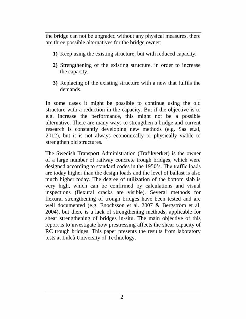
be illustrated by a real life example. Imagine a book shelf filled with
books. A strong person can lift the entire horisontal row of books by
applying a horisontal force, i.e. pressing them against each other,
which will increase the friction between the books and the row will
act as an entity. If the horisontal force is decreasing, the books will
start to slide down due to gravity, and when the horisontal force is
small enough, the friction won’t be able to resist the dead load of the
books and the row will finally collapse.
The same theory applies on concrete structures. By introducing a
horisontal force, caused by e.g. prestressing tendons, the shear
capacity and also the flexural resistance will increase.
Figure 1.2 – Illustration of strengthening method.

4
2. Test setup
Two concrete specimens were tested in order to investigate the
behaviour of RC trough bridges, transversally prestressed with
internal unbonded steel tendons. The specimens were designed in
resemblance to the design drawings of existing railway trough
bridges from the 1950’s, but reduced to a scale of 1/3. One
specimen, B1, was unstrengthened and used as a reference, while
the other one, B2, was strengthened by post tensioning three
transversal unbonded internal steel tendons, denoted N in Figure
2.1. The tendons were put inside cast in plastic ducts, located at mid
height of the slab and the post tensioning was conducted by
hydraulic jacks. The specimens were placed on four spherical
supports and the test setup with dimensions is shown in Figures 2.1
and 2.2.
1040 115 115115 115
110
110
100
85
3N 3N
500
P
P/2 P/2
A-A
B-B
P
110NN
1001500
N
Figure 2.1 – Test setup.

5
2.1. Loading and monitoring
Both specimens were subjected to two monotonic, deformation
controlled line loads, as shown in Figure 2.1. Loading was
conducted by a deformation controlled hydraulic jack until failure at
a constant deformation rate of 0.01 mm/s, and the load was
distributed by one transverse steel beam placed on two longitudinal
steel beams.
Displacements, rotation and global curvature were monitored by
linear variable differential transducers (LVDTs). Electrical
resistance strain gauges measured the strain levels in the internal
steel reinforcement from which local curvature was calculated. Load
cells, see Figure 2.4, were used to measure the load in the
prestressing system.
A
A
B B
1500100 100
1500
Plane
P/L
P/L
Supports
Figure 2.2 – Test setup.

6
2.2. Test bridge geometry
The geometrical data of the test specimen are shown in Figures 2.1
and 2.2. The internal reinforcement, shown in Figure 2.3, consisted
of deformed steel bars with diameters of 6, 8 and 10 mm. The
strengthening system consisted of three steel tendons, built up by
seven strands with a total diameter of 9.6mm, located at mid height
of the bottom slab, as shown in Figure 2.1. One tendon was located
at the longitudinal mid section and the two remaining tendons were
located at a distance of 375 mm on each side of the mid section.
Figure 2.3 – Internal reinforcement and location of strain
gauges.
2.3. Material properties
The targeted concrete class was C30/37, but tested concrete
compressive strengths were 39 MPa and 43 MPa for the
unstrengthened and strengthened specimen, respectively.
Corresponding concrete tensile strengths for the unstrengthened and
strengthened specimen were 2.7 MPa and 3.1 MPa, respectively.
Concrete strength was tested using 150 mm cubes, and concrete
compressive-, fc, and tensile, ft, strength were calculated using
empirical relationships between these quantities and the cubes’
measured cube-, fcu, and splitting, ft,sp, strengths. The concrete
strengths are summarized in Table 2.1.
- Strain gauge
7
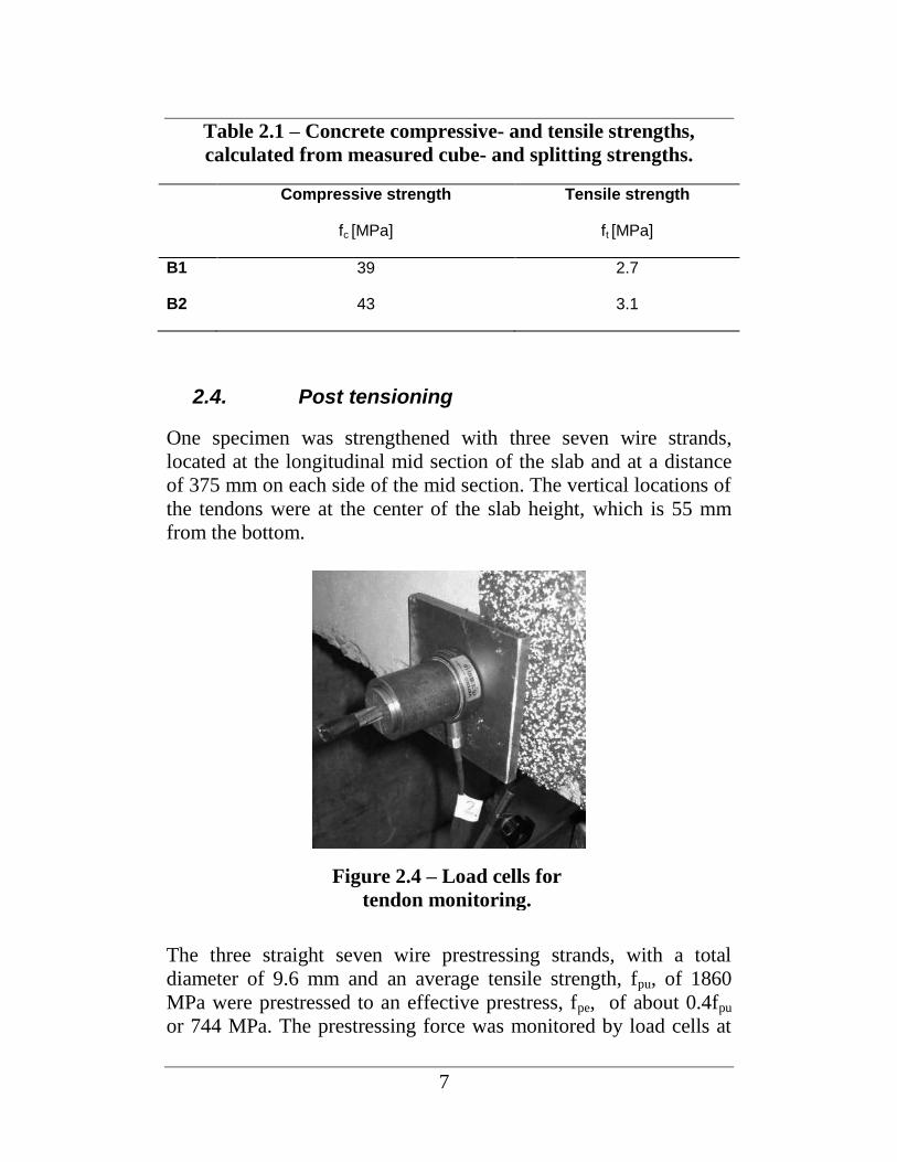
Table 2.1 – Concrete compressive- and tensile strengths,
calculated from measured cube- and splitting strengths.
Compressive strength
fc [MPa]
Tensile strength
ft [MPa]
B1 39 2.7
B2 43 3.1
2.4. Post tensioning
One specimen was strengthened with three seven wire strands,
located at the longitudinal mid section of the slab and at a distance
of 375 mm on each side of the mid section. The vertical locations of
the tendons were at the center of the slab height, which is 55 mm
from the bottom.
The three straight seven wire prestressing strands, with a total
diameter of 9.6 mm and an average tensile strength, fpu, of 1860
MPa were prestressed to an effective prestress, fpe, of about 0.4fpu
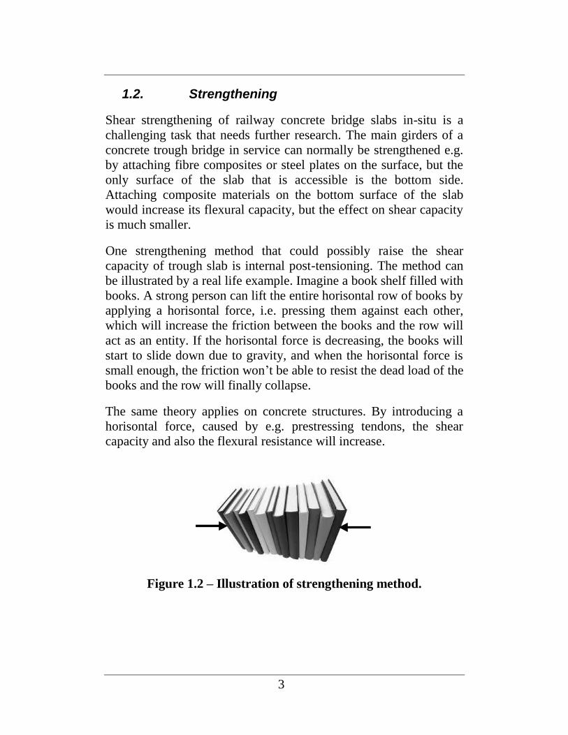
or 744 MPa. The prestressing force was monitored by load cells at
Figure 2.4 – Load cells for
tendon monitoring.

8
each tendon and the post tensioning procedure was a stepwise
prestressing of one tendon at the time, starting with the central
tendon and followed by the outer tendons. Tendon stresses,
calculated from the tendon forces, are shown in Figure 4.9.
Figure 2.5 – Three tendons were used for strengthening of
specimen T2.
9
3. Calculations
3.1. Introductory example
The following example illustrates how prestressing affects the strain
in the internal reinforcement. By introducing a prestress to a
concrete slab, the strain levels in the longitudinal reinforcement will
decrease, increasing the flexural capacity of the slab.
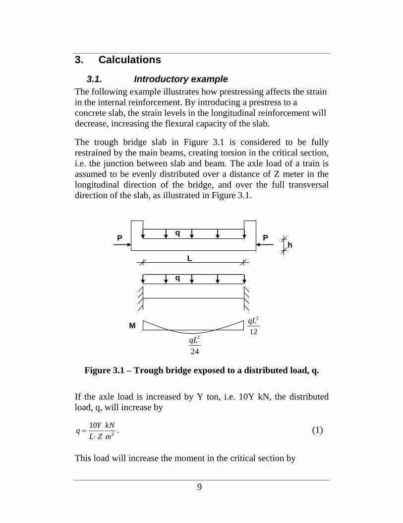
The trough bridge slab in Figure 3.1 is considered to be fully
restrained by the main beams, creating torsion in the critical section,
i.e. the junction between slab and beam. The axle load of a train is
assumed to be evenly distributed over a distance of Z meter in the
longitudinal direction of the bridge, and over the full transversal
direction of the slab, as illustrated in Figure 3.1.
P P
L
q
12
2qL
24
2qL
q
M
h
Figure 3.1 – Trough bridge exposed to a distributed load, q.
If the axle load is increased by Y ton, i.e. 10Y kN, the distributed
load, q, will increase by
2
10
m
kN
ZL
Yq
. (1)
This load will increase the moment in the critical section by

10
Z
LYLqM
12
10
12
2
. (2)
The stress distribution in the cross section is illustrated in Figure 3.2
h
σ
M
Figure 3.2 – Stress distribution in the cross section.
Equilibrium in the section gives
6122
22 hhM
(3)
By inserting Equation (2) into Equation (3), the stress can be
expressed as
22
10
hZ
LY
. (4)
If the axle load is increased by 5 ton, the length of the bridge is 3m,
the height of the bridge is 0.3m and the loads are distributed over
1m in the longitudinal direction, the distributed load will be:
mZ
mh
mL
tonY
1
3.0
3
5
2
7.1613
5010
m
kN
ZL
Yq
(5)
The corresponding stress will be
kPahZ
LY833
3.012
350
2
1022
(6)

11
By introducing a prestressing force, P, the stresses obtained by the
increased axle load can be eliminated. The required prestressing
force, required to compensate for the stress increase of 833kPa is
calculated in Equation (7), below.
mkNhPL /2508333.0 (7)
A prestressing force of 250kN/m will compensate for the 5 ton
increased axle load. If seven wire prestressing strands with the
following properties are used
MPaf
mmA
mm
P
P
700
100
9.122
one strand will provide a prestressing force of
MNAfP PP 07.0100700 (8)
Required distance between prestressing strands is given by Equation
(9).
mP
P
cc
L
28.025.0
07.0 (9)
An increased axle load of 5 ton could, according to the example, be
compensated by prestressing strands with a spacing of 0.28m and an
effective prestressing force of 70 kN/strand. In this example, the
nominal area of the strands are 100mm2, but there are larger strands
that could be more appropriate for this application.

12
3.2. Shear design
The shear capacity was calculated according to beam theory in three
design codes;
The European design code Eurocode 2, (CEN, 2004)
The Canadian design code CSA A23.3-04, (CSA, 2004)
The Swedish design code BBK 04, (Boverket, 2004)
CSA and BBK are both based on the addition principle, where the
total shear resistance, VR, is calculated as the sum of the shear
strengths of concrete, VC, the shear reinforcement, VS, and the
prestressing VP.
PSCR VVVV (10)
In order to provide a safe structure, the total shear resistance, VR,
must be greater than the shear forces, VE, resulting from all loads
acting on the structure as shown in equation (11).
ER VV (11)
Eurocode takes on a slightly different approach. If the specimen
contains shear reinforcement, the resistance of the concrete is
neglected and the shear capacity is given as the resistance of the
stirrups. In the case of no shear reinforcement, the shear resistance
is given as the resistance of concrete where potential prestressing is
included.
The test specimens in this report had no shear reinforcement,
meaning that the shear strength was governed by the shear capacity
of concrete and the contribution from prestressing. The design
calculations are shortly described in the following sections.

13
3.2.1. Eurocode 2
The general procedure for shear design of concrete structures is
presented in chapter 6.2 of Eurocode 2. The design value for the
shear resistance is given by equation (12).
dbσk)fρ(kCV wcpcklRd,cRd,c
1
31
100 (12)
with a minimum of:
dbσkVV wcpRd,c 1min (13)
As seen in equation (12), the shear capacity contribution, provided
by the prestress is included in the shear capacity of the concrete. But
the prestress can easily be separated into equation (14).
dbσkV wcpRd,c 1 (14)
The values for k , 1k , Rd,cC and minV can be found in the National
Annex for each country, but the recommended values are
0.2200
1 d
k (15)
15.01 k (16)
c
Rd,cC
18.0 (17)
21
23
min 035.0 ckfkV (18)
where
c is the partial factor, which can be chosen as 1.2 or 1.5,
depending on the design situation

14
ckf is the characteristic compressive cylinder strength of concrete
at 28 days.
wb is the smallest width of the cross-section in the tensile area.
d is the effective depth of a cross-section.
020.db
Aρ
w
sl
l
(19)
slA is the area of the tensile reinforcement, which extends
dlbd beyond the section considered.
The stress, caused by prestressing is
cd
c
Edcp f
A
Nσ 2.0 [MPa] (20)
where
EdN is the axial force in the cross section due to loading or
prestressing.
cA is the area of the concrete cross section.
3.2.2. CSA
The general procedure for shear design of concrete structures is
presented in chapter 11.3 of CSA A23.3-04. The design value for
the shear resistance is given by the following equation
PvwCcR VdbfV (21)
where
c is the resistance factor for concrete. Normally it is taken as
0.65.

15
is the strength reduction factor to account for low density
concrete. For normal density concrete, its value is 1.
is the factor for accounting for the shear resistance of cracked
concrete. Its value is normally between 0.1 and 0.4.
Cf is the specified compressive strength of concrete.
wb is the effective web width. For rectangular beams, it is the
width of the beam. For flanged beams, it is the width of the
web of the beam.
vd is the effective shear depth. It is taken as the greater of 0.9d or
0.72h, where d is the distance from the extreme compression
fiber to the centroid of the tension reinforcement, and h is the
overall depth of the cross-section in the direction of the shear
force.
pV is a component in the direction of the applied shear of the
effective prestressing force factored with p .
p is the resistance factor for prestressing steel, 0.9 for
prestressing tendons.
3.2.3. BBK
The general procedure for shear design of concrete structures is
presented in chapter 3.7 of BBK 04. The design value for the shear
resistance is given by the following equation.
PSCR VVVV (22)
The shear resistance of the concrete is calculated as
vwC fdbV (23)

16
where
wb is the smallest web width in the region of the effective height
of a cross section.
d is the effective height of a cross section.
vf is the formal shear strength of concrete.
The formal shear strength of concrete is calculated as
ctv ff 50130.0 (24)
where
d1.0m for 9.0
1.0md0.5m for 4.03.1
0.5md0.2m for 6.1
0.2md for 4.1
d
d (25)
02.00
db
A
w
s (26)
ctf is the design value for the tensile strength of concrete.
0sA is the smallest area of the flexural tensile reinforcement in the
zone between for maximum moment and zero moment .
The shear resistance of the prestressing can be calculated as
min
0
2.1
dn
dP
M
MVV
(27)

17
where
dM is the flexural moment cauced by external loads.
0M is the moment which combined with the tensile force, cauces
zero strains.
n is a safety factor.
The shear resistance of the concrete and the prestressing is limited
to
cmctwPC fdbVV 3.0 (28)
where
cm is the average compressive stress in the uncracked cross-
section, cauced by effective tensile force or normal force,
divided by An 2.1 .
3.3. Flexural design
The flexural capacity of the cross-section shown in Figure 3.3 below
is determined by defining the equilibrium equation’s (29) and (33).
P
FS
F’S
FC
M
0.8x 0.4x
AS
A’S x d’
b
d h
ε’S
εC
εS
Figure 3.3 – Forces acting on a prestressed cross section.

18
Assuming yielding in the tensile reinforcement, the horizontal
equilibrium equation in the ultimate limit state will be
0' SSC FPFF (29)
FC is the compressive force in the concrete, F’S is the force in the
compressive reinforcement, P is the prestressing force and FS is the
force in tensile reinforcement. By introducing Hooke’s law into
Equation (29), the equilibrium expression at ultimate limit state can
be written as
0''8.0 SstSSScc AfPAEbxf (30)
where
ccf is the compressive stress of concrete,
b is the width of the cross section,
S' is the strain in the compressive reinforcement,
SE is the elastic modulus for steel,
SA' is the area of the compressive steel,
P is the prestress,
stf is the yield strength of the tensile reinforcement and
SA is the area of the tensile reinforcement
The distance to the neutral layer, x, can be solved with the following
equation
1
2
C
Cx
(31)
where
SstSSS
cc
AfPAEC
bfC
''
8.0
2
1
(32)

19
Through moment equilibrium around the concrete resultant force,
FC, which is assumed to be located at x4.0 at ultimate limit state, the
following expression is obtained
0'4.0'4.02
4.0
MdxFx
hPxdF SS (33)
where
d is the distance to the tensile reinforcement,
'd is the distance to the compressive reinforcement and
M is the moment caused by applied loads at ultimate limit state.
The moment in Equation (33) is determined as
xdFxh
PxdFM SS 4.0'4.02
4.0
(34)
By introducing Hooke’s law into Equation (34), the moment
capacity can be calculated as
xdAExh
PxdAfM SSSSSst 4.0'''4.02
4.0
(35)
For a cross section without prestress, the flexural capacity is
determined by setting the prestressing force P to zero in Equation
(29) – (35).
3.4. Curvature
Two typess of curvature are presented in this report;
Global curvature
Local Curvature
20
The Global curvature was determined by measuring the
displacement deviation between two points along the longitudinal
central line of the test specimen, where the horizontal spacing
between the points are known. Strain gauges, attached on the
internal reinforcement, were used for capturing the local curvature.
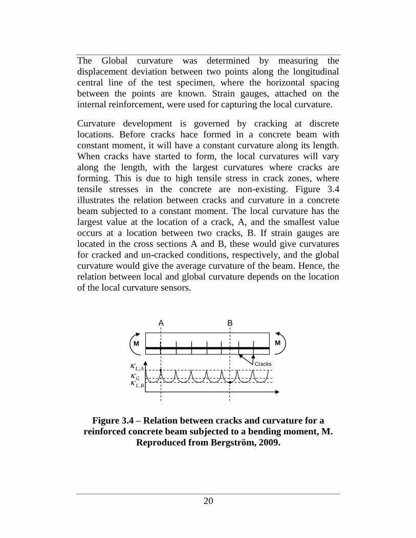
Curvature development is governed by cracking at discrete
locations. Before cracks hace formed in a concrete beam with
constant moment, it will have a constant curvature along its length.
When cracks have started to form, the local curvatures will vary
along the length, with the largest curvatures where cracks are
forming. This is due to high tensile stress in crack zones, where
tensile stresses in the concrete are non-existing. Figure 3.4
illustrates the relation between cracks and curvature in a concrete
beam subjected to a constant moment. The local curvature has the
largest value at the location of a crack, A, and the smallest value
occurs at a location between two cracks, B. If strain gauges are
located in the cross sections A and B, these would give curvatures
for cracked and un-cracked conditions, respectively, and the global
curvature would give the average curvature of the beam. Hence, the
relation between local and global curvature depends on the location
of the local curvature sensors.
AL,
BL, G
Cracks
M M
A B
Figure 3.4 – Relation between cracks and curvature for a
reinforced concrete beam subjected to a bending moment, M.
Reproduced from Bergström, 2009.
21
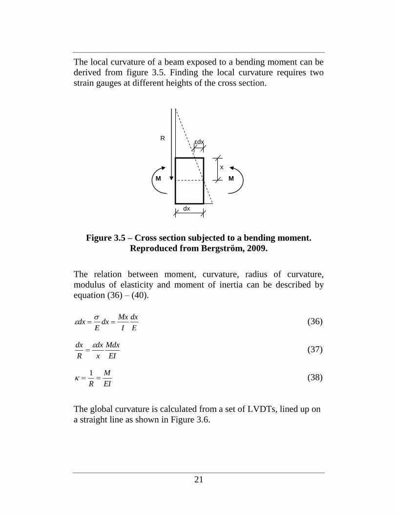
The local curvature of a beam exposed to a bending moment can be
derived from figure 3.5. Finding the local curvature requires two
strain gauges at different heights of the cross section.
R
M M
εdx
x
dx
Figure 3.5 – Cross section subjected to a bending moment.
Reproduced from Bergström, 2009.
The relation between moment, curvature, radius of curvature,
modulus of elasticity and moment of inertia can be described by
equation (36) – (40).
E
dx
I
Mxdx
Edx
(36)
EI
Mdx
x
dx
R
dx (37)
EI
M
R
1 (38)
The global curvature is calculated from a set of LVDTs, lined up on
a straight line as shown in Figure 3.6.

22
Figure 3.4 – Calculating global curvature. Reproduced from
Bergström, 2009.
Equations for global curvature are represented by equation (39) –
(41).
20
iki
KKKy
(39)
0yK jki (40)
22
2
82
4
2
Lxx
ki
kiikki
kiki
(41)
23
4. Results
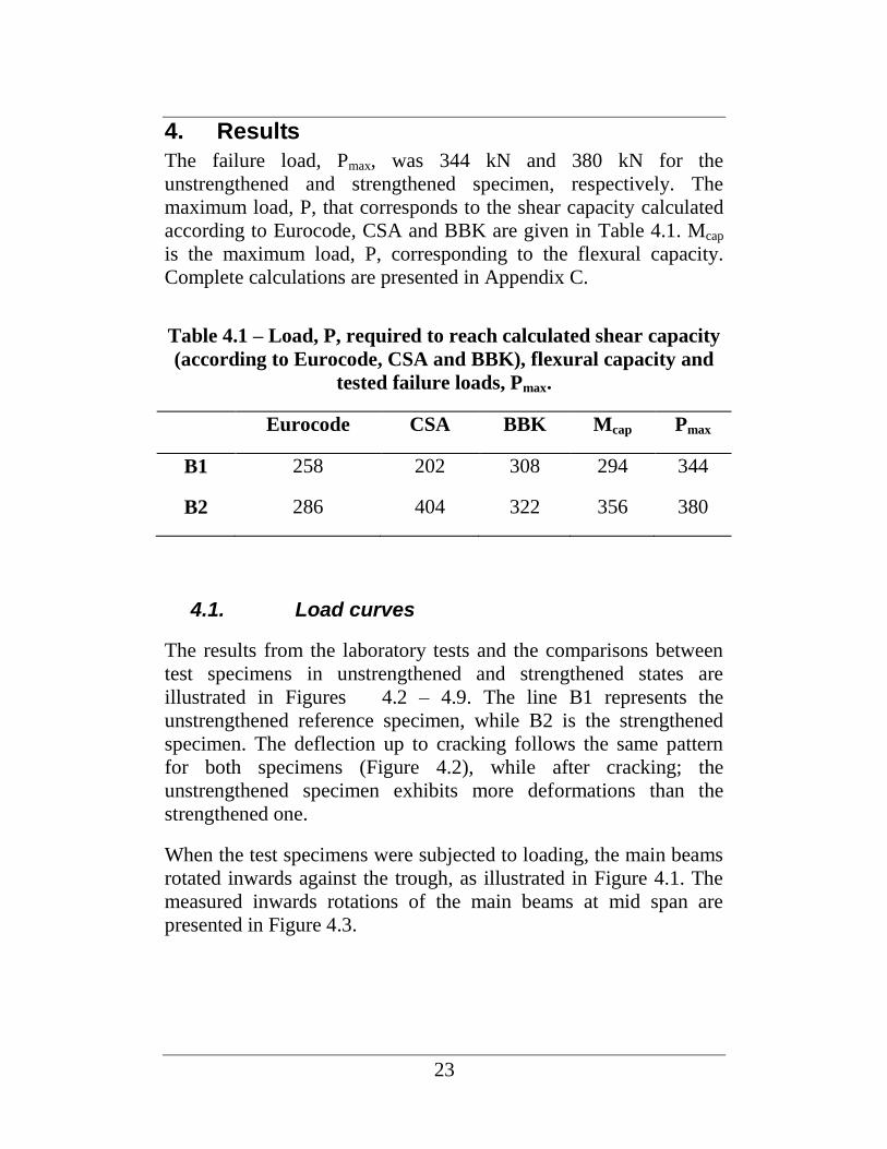
The failure load, Pmax, was 344 kN and 380 kN for the
unstrengthened and strengthened specimen, respectively. The
maximum load, P, that corresponds to the shear capacity calculated
according to Eurocode, CSA and BBK are given in Table 4.1. Mcap
is the maximum load, P, corresponding to the flexural capacity.
Complete calculations are presented in Appendix C.
Table 4.1 – Load, P, required to reach calculated shear capacity
(according to Eurocode, CSA and BBK), flexural capacity and
tested failure loads, Pmax.
Eurocode CSA BBK Mcap Pmax
B1 258 202 308 294 344
B2 286 404 322 356 380
4.1. Load curves
The results from the laboratory tests and the comparisons between
test specimens in unstrengthened and strengthened states are
illustrated in Figures 4.2 – 4.9. The line B1 represents the
unstrengthened reference specimen, while B2 is the strengthened
specimen. The deflection up to cracking follows the same pattern
for both specimens (Figure 4.2), while after cracking; the
unstrengthened specimen exhibits more deformations than the
strengthened one.
When the test specimens were subjected to loading, the main beams
rotated inwards against the trough, as illustrated in Figure 4.1. The
measured inwards rotations of the main beams at mid span are
presented in Figure 4.3.
24
P/2 P/2
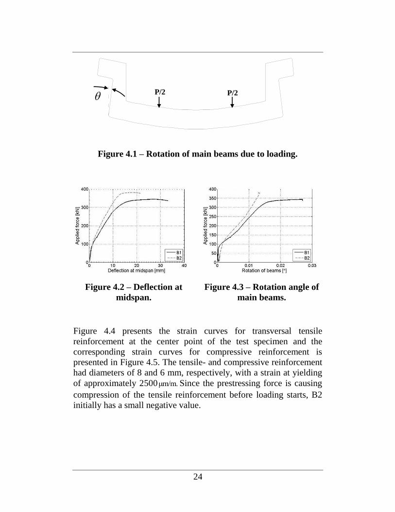
Figure 4.1 – Rotation of main beams due to loading.
Figure 4.2 – Deflection at
midspan.
Figure 4.3 – Rotation angle of
main beams.
Figure 4.4 presents the strain curves for transversal tensile
reinforcement at the center point of the test specimen and the
corresponding strain curves for compressive reinforcement is
presented in Figure 4.5. The tensile- and compressive reinforcement
had diameters of 8 and 6 mm, respectively, with a strain at yielding
of approximately 2500μm/m. Since the prestressing force is causing
compression of the tensile reinforcement before loading starts, B2
initially has a small negative value.

25
Strains were measured in bent up reinforcement bars, with a
diameter of 8 mm, at the junction of the slab and the main girders.
Figure 4.6 illustrates the strain readings from the bent up
reinforcement at mid height of the slab.
Figure 4.6 – Strain in bent up reinforcement.
Figure 4.4 – Strain in tensile
reinforcement.
Figure 4.5 – Strain in
compressive reinforcement.
26
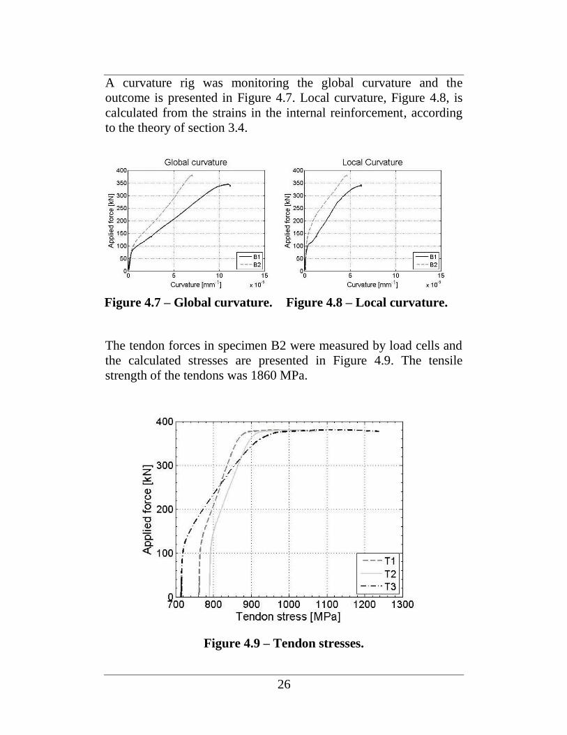
A curvature rig was monitoring the global curvature and the
outcome is presented in Figure 4.7. Local curvature, Figure 4.8, is
calculated from the strains in the internal reinforcement, according
to the theory of section 3.4.
The tendon forces in specimen B2 were measured by load cells and
the calculated stresses are presented in Figure 4.9. The tensile
strength of the tendons was 1860 MPa.
Figure 4.9 – Tendon stresses.
Figure 4.7 – Global curvature. Figure 4.8 – Local curvature.

27
4.2. Crack patterns
The cracks were highlited by a black pen in order to easier see the
pattern. The crack patterns of specimen B1 and B2 are shown in
Figure 4.10 and 4.11, respectively. There are two major- and several
minor flexural cracks appearing in the region between the line loads
and main girders of the unstrengthened specimen.
Figure 4.10 – Crack pattern of specimen B1.

28
After removing the prestress of B2, one major flexural crack opened
up, as seen in Figure 4.11.
Figure 4.11 – Crack pattern of specimen B2 after removing the
prestress.
29
5. Analysis and Discussion
Transversal post tensioning has a positive effect on the behaviour of
concrete trough bridges as seen in the laboratory test results
presented in Figure 4.2 – 4.9. The deformations are clearly
reduced in terms of decreased vertical displacements of the slabs
and less rotation of the main girders. In an in-situ situation, when
the trough is filled with ballast, loading will force the main beams to
rotate inwards, but the rotation will be prohibited by the ballast
inside of the trough. Instead of rotating the beams, the loading will
create torsion at the junction of the slab and the main girders. The
effect of prestressing is decreased rotation of the main girders, as
seen in Figure 4.3.
Figure 4.4 shows that the strain levels in the tensile reinforcement
are also significantly decreased after prestressing, which should
render in an increased flexural capacity. This is described in section
3.3.
The main objective of the laboratory tests was to investigate how
the prestressing affected the transversal shear behaviour and if the
capacity of the slab could be increased. The largest shear forces, in
the current test setup, appeared in the exterior side of the line loads,
i.e. between line load and beam, see Figure 4.3. Since there was no
shear reinforcement in the slab, the shear stresses were best
represented by the strain levels in the bent up reinforcement at the
junction of the slab and the main girders as seen in Figure 4.6. The
strains in the bent up bars were dramatically affected by post-
tensioning, i.e. the strain was significantly smaller in the
strengthened specimen. The post tensioned specimen also exhibited
compression before any tension could be detected in the bent up
bars. The reduced strains in the bent up bars, for the strengthened
specimen, indicate a relief in shear stress and thus an increase in the
shear capacity.
The tendons were prestressed up to an effective prestress of about
40% of the tendon capacity, generating a total prestressing force of
124 kN for the three tendons. It would threfore be possible to
increase the prestressing force, which will result in even higher load
carrying capacities. Figure 5.1 illustrates how the load capacities,

30
calculated from the shear capacities according to Eurocode and
BBK, are affected by increasing the prestress.
Eurocode and BBK starts with load capacities of 258 and 308 kN,
respectively for the unstrengthened beam. For a prestress of 124 kN
(red dashed line in Figure 5.1), the load capacities has increased up
to 286 and 322 kN for Eurocode and BBK, respectively. As seen in
Figure 5.1, the prestress impact on shear capacity is higher for
Eurocode, i.e. the slope of the blue line is steeper. When the
prestress approaches 500 kN, the maximum load, calculated from
the shear capacity according to BBK and Eurocode, coincides at
approximately 375 kN.
Figure 5.1 – Effect of increasing the prestress.

31
6. Future research
Transversal post tensioning of concrete trough bridges has a
stiffening effect on the structure, which can be interpreted from
Figures 4.2 – 4.9 above. The deflections, as well as the
reinforcement strains, are decreased by this strengthening method.
As seen in Figure 4.6, strains in the bent up bars are dramatically
affected by post-tensioning. The strain magnitude is vastly
decreased in the strengthened specimen compared to the
unstrengthened one, and the post tensioned specimen exhibits
compression before any tension takes place.
The reduced strains in the bent up bars, for the strengthened
specimen, indicate a relief in shear stress and thus an increase in the
shear capacity. Further tests are required to confirm the test results
presented in this report.
Field tests are also needed in order to test the actual behavior of, and
strengthening effects on a trough bridge under live loads. Field tests
are currently beeing planned.

32
33
7. References
Bell, B., (2004), “D1.2 European Railway Bridge Demography”,
European FP 6 Integrated project "Sustainable Bridges",
Assessment for Future Traffic Demands and Longer Lives,
http://www.sustainablebridges.net, accessed date 10 January 2012.
Sas, G., Blanksvärd, T., Elfgren, L., Enochsson, O. and Täljsten, B.,
(2012), “Photographic strain monitoring during full scale failure
testing of Örnsköldsvik Bridge”, Journal of Structural Health
Monitoring, 2012, (in press).
Enochsson, O., Nordin, H., Täljsten, B., Carolin, A., Kerrouche, A.,
Norling, O., Falldén, C., (2007), “Field test – Strengthening of the
Örnsköldsviks Bridge with near surface mounted CFRP rods”,
deliverable D6.3 within Sustainable Bridges, 55 p.
Bergström, M., Danielsson, G., Johansson, H. & Täljsten, B. (2004):
“Mätning på järnvägsbro över Fröviån”, Technical Report,
Technical University of Luleå, Luleå, Sweden, 73 p.
Bergström, M., (2009), “Assessment of existing concrete bridges:
bending stiffness as a performance indicator”, Doctoral thesis,
Luleå University of Technology, Luleå (Sweden), 102pp, ISBN
978-91-86233-11-2
CEN, (2008), “EN 1992-1-1:2004 Eurocode 2: Design of concrete
structures - Part 1-1: General rules and rules for buildings“, CEN:
European Committee for Standardization, Brussels (Belgium).
Boverket, (2004), ”Boverkets handbok om betongkonstruktioner:
BBK 04”, 3rd edition, Boverket, Karlskrona (Sweden), ISBN 91-
7147-816-7.
CSA, (2004), “CSA-A23.3-04 (R2010) - Design of Concrete
Structures”, CSA: Canadian Standards Association, Mississauga
(Canada).

34
35
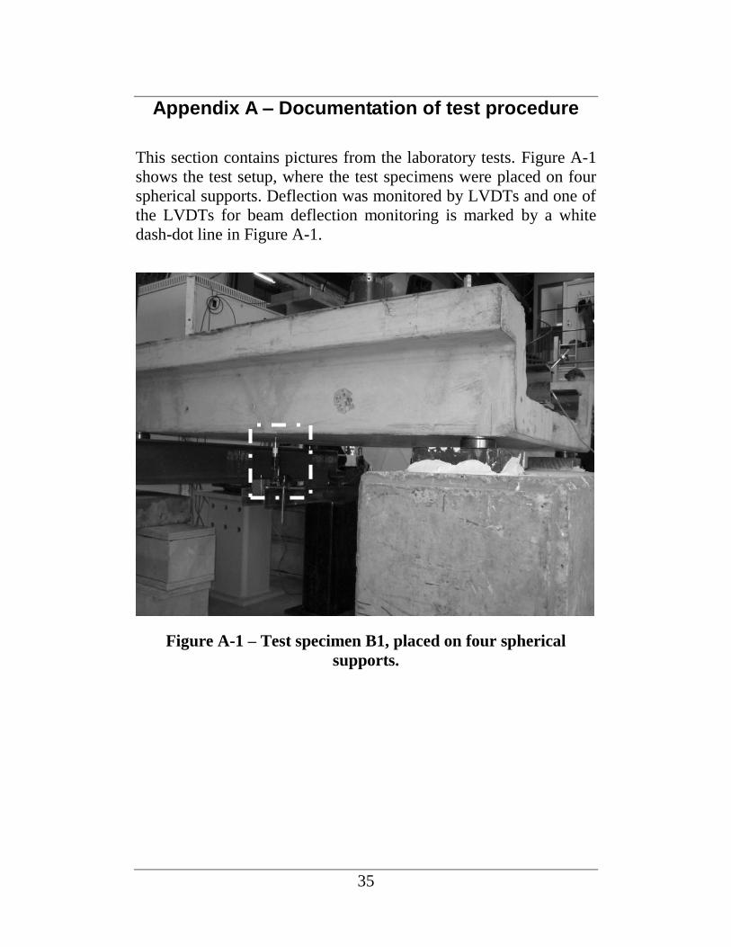
Appendix A – Documentation of test procedure
This section contains pictures from the laboratory tests. Figure A-1
shows the test setup, where the test specimens were placed on four
spherical supports. Deflection was monitored by LVDTs and one of
the LVDTs for beam deflection monitoring is marked by a white
dash-dot line in Figure A-1.
Figure A-1 – Test specimen B1, placed on four spherical
supports.

36
The beam rotations were calculated from the displacements of the
beams, which were monitored by two LVDTs, one horizontal and
one vertical. Location of rotation LVDTs are marked by black and
white dash-dot lines in Figure A-2.
Figure A-2 – Monitoring of beam rotation.
37
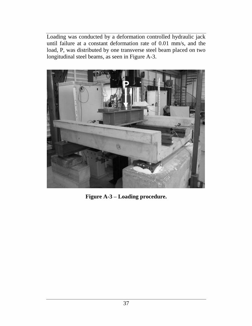
Loading was conducted by a deformation controlled hydraulic jack
until failure at a constant deformation rate of 0.01 mm/s, and the
load, P, was distributed by one transverse steel beam placed on two
longitudinal steel beams, as seen in Figure A-3.
Figure A-3 – Loading procedure.
P

38
Specimen B2, was strengthened by transversal post-tensioning of
the slab, as shown in Figure A-4. Three unbonded tendons were
used in this procedure, one located at the midsection and the others
at a distance of 375 mm on each side of the midsection. The vertical
distance to the tendons was 55 mm from the bottom side.
Figure A-4 – Prestressing strands.
39
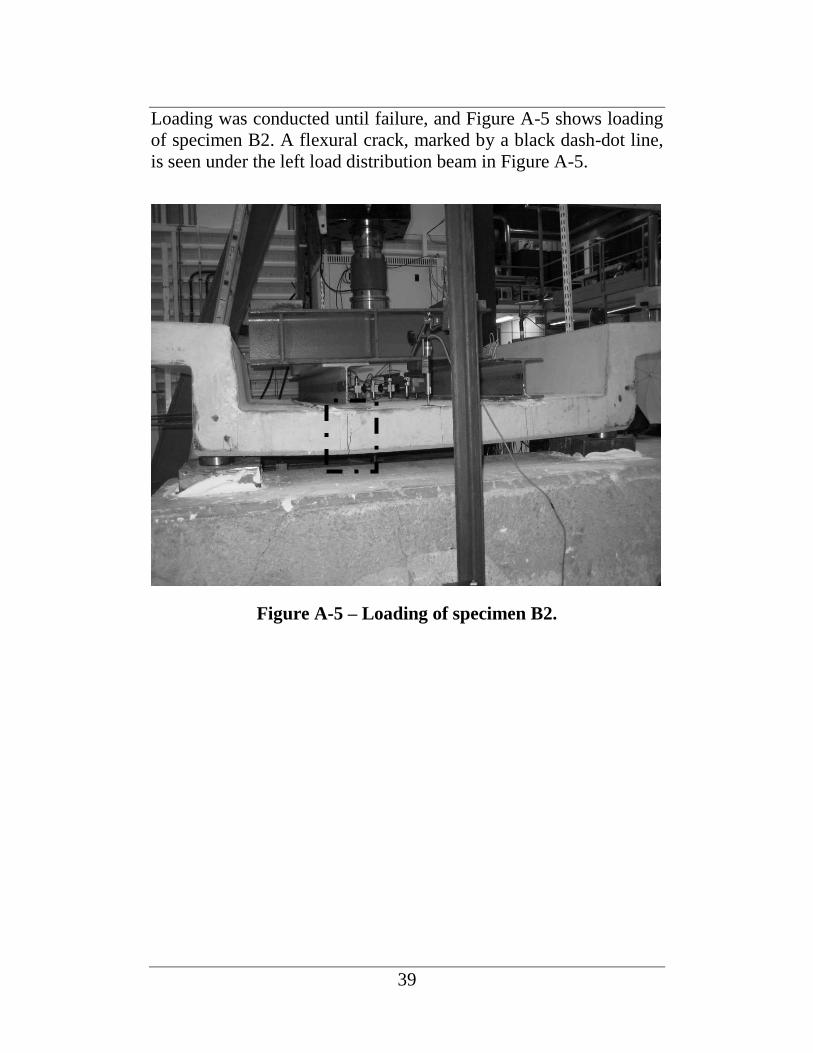
Loading was conducted until failure, and Figure A-5 shows loading
of specimen B2. A flexural crack, marked by a black dash-dot line,
is seen under the left load distribution beam in Figure A-5.
Figure A-5 – Loading of specimen B2.

40
The tendon forces were monitored by load cells on the end of each
tendon, as seen in Figure A-6. The tendon stresses were then
calculated from the force readings.
Figure A-6 – Monitoring of tendon forces with load cells.

41
A curvature rig was placed between the line loads, along the
midsection, as shown in Figure A-7. The curvature rig consisted of
5 LVDTs.
Figure A-7 – Curvature rig at mid section.

42

43
Appendix B – Test results
Appendix B contains the load curves from the laboratory tests.
B.1 Deformation curves
Deformation curves presented in this appendix includes
displacement-, rotation- and curvature measurements. Figure B-1
illustrates the locations and numbering of the linear variable
differential differential transducers, used for deflection monitoring.
A
A
B B
1500100 100
15
00
PlaneSupports
LVDTs
321
A
B
Figure B-1 – Location and numbering of linear variable
differential transducers (LVDTs) for vertical displacement
monitoring.

44
The midspan displacements were monitored by LVDT 1, 2 and 3 in
Figure B-1 and the results for specimen B1 and B2 are presented in
Figure B-2 and B-3, respectively.
Figure B-2 – Deflection at
midspan, specimen B1.
Figure B-3 – Deflection at
midspan, specimen B2.
As the loading increases, the main beams were rotating inwards, as
shown in Figure B-4. The rotation angle is presented in Figure B-5.
θ P/2 P/2
Figure B-4 – Rotation of main beams, due to loading.

45
Figure B-5 – Rotation of main beams.
The deflections were monitored at point A and B in figure B-1. The
results from these measurements are presented in Figure B-6 and B-
7 for specimen B1 and B2, respectively.
Figure B-6 – Deflection of main
beams, specimen B1.
Figure B-17 – Deflection of main
beams, specimen B2.

46
The global curvature was measured by a curvature rig, with LVDTs
lined up along the midsection and the local curvature was calculated
from the steel strains. The global curvature is presented in Figure B-
8 and the local curvature is presented in Figure B-9.
Figure B-8 – Global
curvature.
Figure B-9 – Local
curvature.

47
B.2 Strain curves and tendon forces
Strains were monitored by strain gauges, mounted on the internal
reinforcement. Locations and numbering of strain gauges are shown
in Figure B-10.
57.5 260 260
55
55
3 421
7
6
Strain gauge
Figure B-10 – Location and numbering of strain gauges.
Strain in bottom reinforcement of specimen B1 and B2 are
presented in Figure B-11 and B-12, respectively.
Figure B-11 – Strain in tensile
reinforcement, specimen B1.
Figure B-12 – Strain in tensile
reinforcement, specimen B2.

48
Strains measured in top reinforcement of specimen B1 and B2 are
presented in Figure B-13 and B-14, respectively.
Strain levels were also monitored in two levels of the bent up
reinforcement, namely 6 and 7 in Figure B-10. Figure B-15 and B-
16 presents the strains for specimen B1 and B2, respectively.
Figure B-13 – Strain in
compressive reinforcement,
specimen B1.
Figure B-14 – Strain in
compressive reinforcement,
specimen B2.
Figure B-15 – Strain in bent up
reinforcement, specimen B1.
Figure B-16 – Strain in bent
up reinforcement, specimen
B2.
49
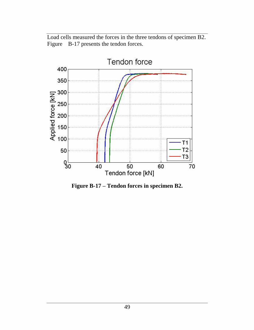
Load cells measured the forces in the three tendons of specimen B2.
Figure B-17 presents the tendon forces.
Figure B-17 – Tendon forces in specimen B2.

50

51
Appendix C – Calculations
C.1 Shear capacity calculations
C.1.1 Eurocode
The shear capacity is calculated as:
dbσk)fρ(kCV wcpcklRd,cRd,c
1
31
100
with a minimum value of
dbσkVV wcpRd,c 1min
The different parts are calculated as:
0.252.286
2001
2001 k
dk
15.01 k
18.01
18.018.0
c
Rd,cC
0200049.0861700
712.
db
Aρ
w
sll
MPafkV ck 542.0300.2035.0035.0 21
23
21
23
min
52
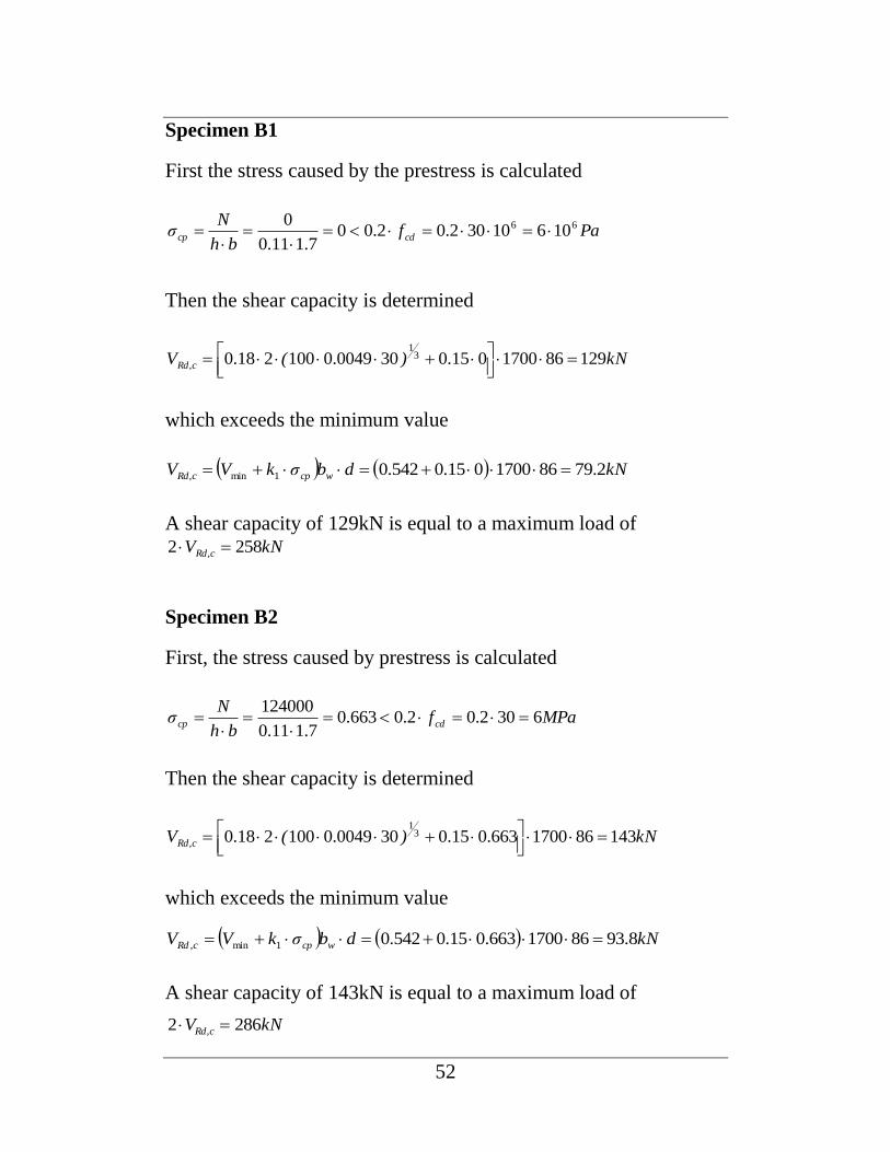
Specimen B1
First the stress caused by the prestress is calculated
Pafbh
Nσ cdcp
66 10610302.02.007.111.0
0
Then the shear capacity is determined
kN)(VRd,c 129861700015.0300049.0100218.0 31
which exceeds the minimum value
kNdbσkVV wcpRd,c 2.79861700015.0542.01min
A shear capacity of 129kN is equal to a maximum load of kNVRd,c 2582
Specimen B2
First, the stress caused by prestress is calculated
MPafbh
Nσ cdcp 6302.02.0663.0
7.111.0
124000
Then the shear capacity is determined
kN)(VRd,c 143861700663.015.0300049.0100218.0 31
which exceeds the minimum value
kNdbσkVV wcpcRd 8.93861700663.015.0542.01min,
A shear capacity of 143kN is equal to a maximum load of
kNVRd,c 2862

53
C.1.2 CSA
The shear capacity is calculated as
PvwCcR VdbfV
where
65.0c
1
MPafC 30
mmbw 1700
mmh
ddv 2.79
2.7911072.0
4.77869.0
72.0
9.0max
21.0
Specimen B1
The shear capacity is
kNVdbfV PvwCcR 10102.7917003021.0165.0
VR does not exceed the maximum allowed resistance
kNVdbfV PvwCcR 65602.7917003065.025.025.0max,
A shear capacity of 101kN is equal to a maximum load of
kNVR 2022
54
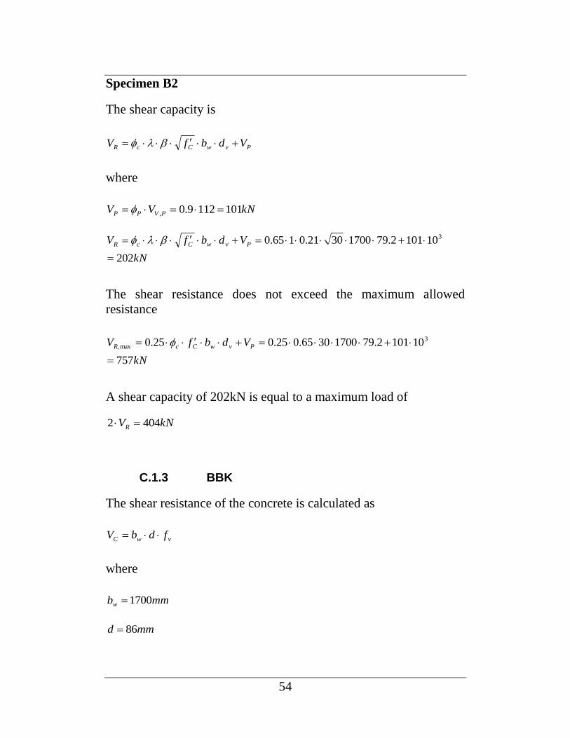
Specimen B2
The shear capacity is
PvwCcR VdbfV
where
kNVV PVPP 1011129.0,
kN
VdbfV PvwCcR
202
101012.7917003021.0165.0 3
The shear resistance does not exceed the maximum allowed
resistance
kN
VdbfV PvwCcR
757
101012.7917003065.025.025.0 3
max,
A shear capacity of 202kN is equal to a maximum load of
kNVR 4042
C.1.3 BBK
The shear resistance of the concrete is calculated as
vwC fdbV
where
mmbw 1700
mmd 86
55
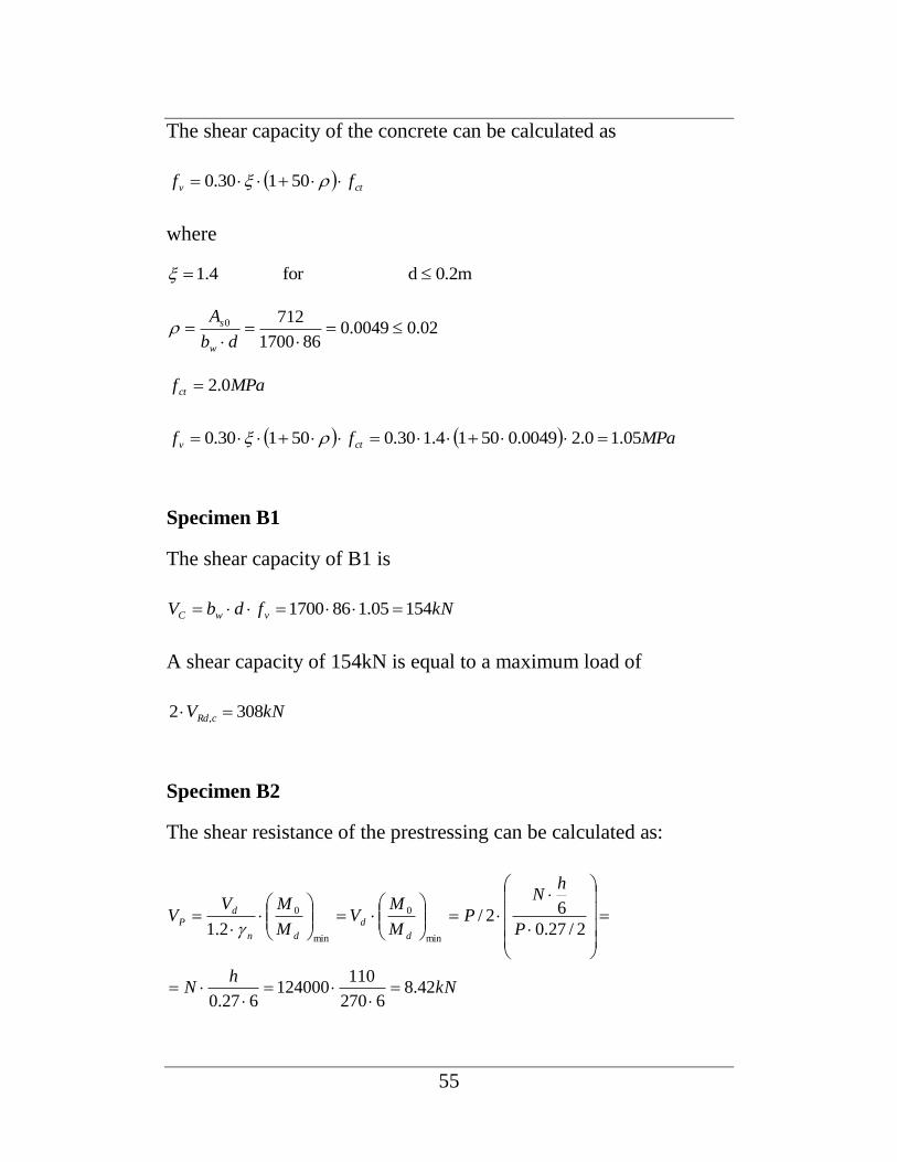
The shear capacity of the concrete can be calculated as
ctv ff 50130.0
where
0.2md for 4.1
02.00049.0861700
7120
db
A
w
s
MPafct 0.2
MPaff ctv 05.10.20049.05014.130.050130.0
Specimen B1
The shear capacity of B1 is
kNfdbV vwC 15405.1861700
A shear capacity of 154kN is equal to a maximum load of
kNVRd,c 3082
Specimen B2
The shear resistance of the prestressing can be calculated as:
kNh
N
P
hN
PM
MV
M
MVV
d
d
dn
dP
42.86270
110124000
627.0
2/27.0
62/2.1
min
0
min
0

56
The shear capacity of B2 is then calculated as
kNVV pC 16142.8153
A shear capacity of 161kN is equal to a maximum load of
kN3221612
C.2 Flexural capacity calculations
Assuming yielding in the tensile reinforcement, the horizontal
equilibrium equation will be:
0' SSC FPFF
which can be developed into:
0''8.0 SstSSScc AfPAEbxf
The distance to the neutral layer, x, can be solved with the following
equation:
1
2
C
Cx
where
408001700308.08.01 bfC cc

57
Specimen B1
S
SSstSSS
C
AfPAEC
'103.77359040
704510036810210'''
6
2
3
2
If a strain of OOO7.0 in the top steel is assumed, the distance to the
neutral layer will be
mmx 1040800
0007.0103.77359040 6
Through moment equilibrium around the concrete resultant force the
following equation is obtained
04.0'4.02
4.0
MxdFx
hPxdF SS
where the moment capacity can be solved as
xdAExh
PxdAfM SSSSSst 4.0'''4.02
4.0
kNm
M
4.29134.023368102100007.0
134.02
1100134.086704500
3
A moment of 29.4kNm is equal to a maximum point load of
kNM
P 2942.0
4.292
2.0
2

58
Specimen B2
S
SSstSSS
C
AfPAEC
'103.77483040
70451012400036810210'''
6
2
3
2
If a strain of OOO7.0 in the top steel is assumed, the distance to the
neutral layer will be
mmx 1340800
0007.0103.77483040 6
Through moment equilibrium around the concrete resultant force the
following equation is obtained
04.0'4.02
4.0
MxdFx
hPxdF SS
where the moment can be solved as
xdAExh
PxdAfM SSSSSst 4.0'''4.02
4.0
kNm
M
6.35134.023368102100007.0
134.02
110124000134.086704500
3
A moment of 35.6kNm is equal to a maximum point load of
kNM
P 3562.0
6.352
2.0
2