_____________________________________________________________________________________Richard Valliant is a mathematical statistician in the Office of Survey Methods Research, U.S. Bureau ofLabor Statistics. He thanks the referees for their useful comments. Any opinions expressed are those ofthe author and do not reflect policy of the Bureau of Labor Statistics.

Post-Stratification and Conditional Variance Estimation

Richard ValliantU.S. Bureau of Labor Statistics

Room 2126 , 441 G St. NWWashington DC 20212

February 1992

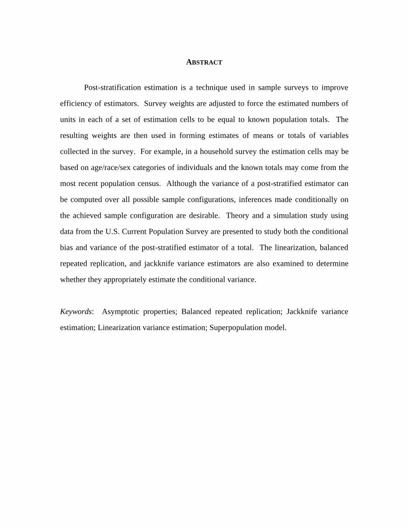
ABSTRACT

Post-stratification estimation is a technique used in sample surveys to improve

efficiency of estimators. Survey weights are adjusted to force the estimated numbers of

units in each of a set of estimation cells to be equal to known population totals. The

resulting weights are then used in forming estimates of means or totals of variables

collected in the survey. For example, in a household survey the estimation cells may be

based on age/race/sex categories of individuals and the known totals may come from the

most recent population census. Although the variance of a post-stratified estimator can

be computed over all possible sample configurations, inferences made conditionally on

the achieved sample configuration are desirable. Theory and a simulation study using

data from the U.S. Current Population Survey are presented to study both the conditional

bias and variance of the post-stratified estimator of a total. The linearization, balanced

repeated replication, and jackknife variance estimators are also examined to determine

whether they appropriately estimate the conditional variance.

Keywords: Asymptotic properties; Balanced repeated replication; Jackknife variance

estimation; Linearization variance estimation; Superpopulation model.

0

1. INTRODUCTION

In complex large-scale surveys, particularly household surveys, post-stratification

is a commonly used technique for improving efficiency of estimators. A clear

description of the method and the rationale for its use was given by Holt and Smith

(1979) and is paraphrased here. Values of variables for persons may vary by age, race,

sex, and other demographic factors that are unavailable for sample design at the

individual level. A population census may, however, provide aggregate information on

such variables that can be used at the estimation stage. After sample selection, individual

units are classified according to the factors and the known total number of units in the cth

cell, Mc , is used as a weight to estimate the cell total for some target variable. The cell

estimates are then summed to yield an estimate for the full population. A variety of

government-sponsored household surveys in the United States use this technique,

including the Current Population Survey, the Consumer Expenditure Survey, the

National Health Interview Survey, and the Survey of Income and Program Participation.

Because post-stratum identifiers are unavailable at the design stage, the number of

sample units selected from each post-stratum is a random variable. Inferences can be

made either unconditionally, i.e. across all possible realizations of the post-strata sample

sizes, or conditionally given the achieved sample sizes. In a simpler situation than that

considered here, Durbin (1969) maintained, on grounds of common sense and the

ancillarity of the achieved sample size, that conditioning was appropriate. In the case of

post-stratification in conjunction with simple random sampling of units, Holt and Smith

(1979) argue strongly that inferences should be conditioned on the achieved post-stratum

sample sizes.

Although conditioning is, in principle, a desirable thing to do, a design-based

conditional theory for complex surveys may be intractable, as noted by Rao (1985). A

useful alternative is the prediction or superpopulation approach which is applied in this

paper to make inferences from post-stratified samples. We will concentrate especially on

1

the properties of several commonly used variance estimators to determine whether they

estimate the conditional variance of the post-stratified estimator of a finite population

total.

Section 2 introduces notation, a superpopulation model that will be used to study

properties of various estimators, and a class of estimators which will be used as the

starting point for post-stratification estimation. Section 3 discusses the model bias and

variance of estimators of the total while sections 4 through 6 cover the linearization,

balanced repeated replication, and jackknife variance estimators. In section 7 we present

the results of a simulation study using data from the U.S. Current Population Survey and

the last section gives concluding remarks.

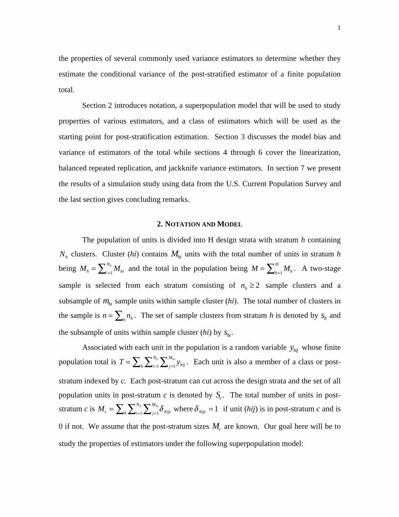
2. NOTATION AND MODEL

The population of units is divided into H design strata with stratum h containing

Nh clusters. Cluster (hi) contains Mhi units with the total number of units in stratum h

being M Mh hii

Nh==Â 1

and the total in the population being M Mhh

H=

=Â 1. A two-stage

sample is selected from each stratum consisting of nh ≥ 2 sample clusters and a

subsample of mhi sample units within sample cluster (hi). The total number of clusters in

the sample is n nhh= Â . The set of sample clusters from stratum h is denoted by sh and

the subsample of units within sample cluster (hi) by shi .

Associated with each unit in the population is a random variable yhij whose finite

population total is T yhijj

M

i

N

h

hih=== ÂÂÂ 11

. Each unit is also a member of a class or post-

stratum indexed by c. Each post-stratum can cut across the design strata and the set of all

population units in post-stratum c is denoted by Sc . The total number of units in post-

stratum c is Mc hijcj

M

i

N

h hijchih= =

== ÂÂÂ d d where 11

1 if unit (hij) is in post-stratum c and is

0 if not. We assume that the post-stratum sizes Mc are known. Our goal here will be to

study the properties of estimators under the following superpopulation model:

2

E y

y y

h h i i j j hij S

h h i i j j hij S h i j S

h h i i j j hij S h i j S

hij c

hij h i j

hic c

hic hic c c

hicc c c

( )

cov( , )

, , , ( )

, , , ( ) ,( )

, , , ( ) ,( )

=

=

= ¢ = ¢ = ¢ Œ

= ¢ = ¢ π ¢ Œ ¢ ¢ ¢ Œ= ¢ = ¢ π ¢ Œ ¢ ¢ ¢ Œ

R

S||

T||

¢ ¢ ¢¢ ¢

m

s

s rt

2

2

0 otherwise . (1)

In addition to being uncorrelated, we also assume that the y's associated with units in

different clusters are independent. The model assumes that units in a post-stratum have a

common mean m c and are correlated within a cluster. The size of the covariances

s rhic hic2 and t hicc¢ are allowed to vary among the clusters and also depend on whether or

not units are in the same post-stratum. The variance specification s hic2 is quite general,

depending on the design stratum, cluster, and post-stratum associated with the unit. All

expectations in the subsequent development are with respect to model (1) unless

otherwise specified.

The general type of estimator of T that we will consider has the form$ $T Thi hii sh h

=ŒÂ g (2)

where g hi is a coefficient that does not depend on the y's,

$T M y y y mhi hi hi hi hij hij shi

= =ŒÂ , and . In common survey practice, the set of g hi is

selected to produce a design-unbiased or design-consistent estimator of the total under

the particular probability sampling design being used. Alternatively, estimator (2) can be

written as

$T K yhic hicci sh h

=  Œ (3)

where K M m m mhic hi hi hic hi hic= g , is the number of sample units in sample cluster (hi)

that are part of post-stratum c, and y y mhic hij hijc hicj shi

=ŒÂ d . If mhic = 0, then define

yhic = 0. There are a variety of estimators, both from probability sampling theory and

superpopulation theory, that fall in this class. Six examples are given in Valliant (1987)

and include types of separate ratio and regression estimators with Mhi used as the

3

auxiliary variable. For example, the ratio estimator has ghi h hii sM M

h

=˛

Error!

Reference source not found., and the regression estimator has

ghih

hh h hs hi hs hi hsi s

N

nn M M M M M M

h

= + - - -˛

12c hc h c h

where M Mh hs and are population and sample means per cluster of the Mhi ' s . Also

included in the class defined by (2) is the Horvitz-Thompson estimator when clusters are

selected with probabilities proportional to Mhi and units within clusters are selected with

equal probability in which case ghi h h hiM n M= b g. Note that, as discussed in section 3,

the estimators defined by (2) are not necessarily model-unbiased under (1).

Next, we turn to the definition of the post-stratified estimator of the total. The

usual design-based estimator of Mc in class (2) is found by using dhijc in place of yhij in

(3) and omitting the sum over c, which gives $M Kc hici sh h

=˛

. The post-stratified

estimator of the total T is then defined as

$ $ $T R Tps cc c= (4)

where $ $R M Mc c c= Error! Reference source not found. and $T K yc hic hici sh h

=˛

. With this

notation the general estimator (3) can also be written as $ $T Tcc= . For subsequent

calculations it will be convenient to write down the model for the set of means

y i shic h, ˛l q implied by model (1):

E y

y y

v h h i i c c

h h i i c c

hic c

hic h i c

hic

hicc

( )

cov( , )

, ,

, ,

=

=

= ¢ = ¢ = ¢

= ¢ = ¢ „ ¢

RS|T|

¢¢¢ ¢

m

t

0 otherwise (5)

where v m mhic hic hic hic hic= + -s r2 1 1b g .

3. MODEL-BIAS AND VARIANCE OF ESTIMATORS OF THE TOTAL

4

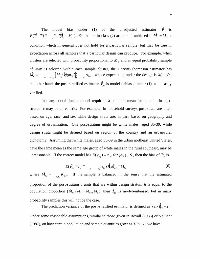
The model bias under (1) of the unadjusted estimator $T is

E T T M Mc c cc( $ ) $- = -m d i. Estimators in class (2) are model unbiased if $M Mc c= , a

condition which in general does not hold for a particular sample, but may be true in

expectation across all samples that a particular design can produce. For example, when

clusters are selected with probability proportional to Mhi and an equal probability sample

of units is selected within each sample cluster, the Horvitz-Thompson estimator has$Mc = M n mh h hii sh hijcj sh hi

b g˛ ˛

d , whose expectation under the design is Mc . On

the other hand, the post-stratified estimator $Tps is model-unbiased under (1), as is easily

verified.

In many populations a model requiring a common mean for all units in post-

stratum c may be unrealistic. For example, in household surveys post-strata are often

based on age, race, and sex while design strata are, in part, based on geography and

degree of urbanization. One post-stratum might be white males, aged 35-39, while

design strata might be defined based on region of the country and an urban/rural

dichotomy. Assuming that white males, aged 35-39 in the urban northeast United States,

have the same mean as the same age group of white males in the rural southeast, may be

unreasonable. If the correct model has E y hij Shij hc c( ) )= ˛m for ( , then the bias of $Tps is

E T T R M Mps hc c hc hci sc h

( $ ) $ $- = -˛m d i (6)

where $M Khc hici sh

=˛

. If the sample is balanced in the sense that the estimated

proportion of the post-stratum c units that are within design stratum h is equal to the

population proportion ( $ $M M M Mhc c hc c= ), then $Tps is model-unbiased, but in many

probability samples this will not be the case.

The prediction variance of the post-stratified estimator is defined as var $T Tps -d i.Under some reasonable assumptions, similar to those given in Royall (1986) or Valliant

(1987), on how certain population and sample quantities grow as H fi ¥ , we have

5

var $ var $T T Tps ps- »d i d i (7)

where » denotes "asymptotically equivalent to." Details are sketched in Appendix A.1.

Consequently, we will concentrate on the estimation of var( $Tps ).

In order to compute the variance, it is convenient to write the post-stratified

estimator as $ $ $Tps hh= ¢R T where $ $ , , $R = ¢R RC1 Kd i,Error! Bookmark not defined.

$ , , ,T K y K yh h h hC hC= ¢ ¢ ¢1 1 Kb g Khc h c hn cK K

h= ¢

1 , ,Kd i, and yhc h c hn cy yh

= ¢1 , ,Kd i. Using the

model for the means yhic given by (5), the variance can be found, as sketched in the

appendix, as

var( $ ) $ $Tps h hh h= ¢ ¢R K V K R (8)

where ¢Kh is the C n Ch· matrix whose cth row is ¢ ¢ ¢ ¢ ¢0 0 K 0 0n n hc n nh h h h, , , ,K Kd i, i.e. ¢Khc is

preceded by c-1 zero row vectors of length nh and followed by C-c such zero vectors.

The matrix Vh is defined as

V

V D D

D V

D V

h

h h h C

h h

hC hC

=

L

N

MMMM

O

Q

PPPP

1 12 1

21 2

1

t t

t

t

L

M O

with V Dhc hic n n hcc hicc n nv

h h h h= =

· ¢ ¢ ·diag and diagb g b gt t where i sh˛ for both V Dhc hcc and t ¢.

A key point is that, although the factors $Rc may be random with respect to the sample

design, they are constant with respect to model (1), so that (8) is a variance conditional

on the values of $Rc.

The variance of the unadjusted estimator $T can be found by minor modification

of the above arguments. Because $ $T hh= T , i.e. the value of $Tps when $Rc =1 for all c,

we have

var( $)T C h hh h C= ¢ ¢1 K V K 1 (9)

where 1C is a vector of C 1's. Note that, if the sample design is such that the post-

stratum factors $Rc each converge to 1, then var $ var $T Tpsdi di and are about the same in

large samples.

6

4. A LINEARIZATION VARIANCE ESTIMATOR

Linearization or Taylor series variance estimators for post-stratified estimators are

discussed for general sample designs by Rao (1985) and Williams (1962). An

application to a complex survey design is given in Parsons and Casady (1985). Our

interest here is in how a linearization estimator, derived from design-based arguments,

performs as an estimator of the approximate conditional variance given by (8). For

clarity and completeness we will sketch the derivation of the estimator for the class of

post-stratified estimators studied here. In a design-based analysis, the product $ $R Tc c is

expanded about the point M Tc c,b g where Tc is the finite population total for post-stratum

c. The usual first-order Taylor approximation to $ $R Tc c is $ $ $ $R T T T T M Mc c c c c c c@ + - . From

this expression it follows that $ %T T dps hii sh h

- @˛

where

%d M y T M mhi hi hi hijccj s hij c c hihi

= -˛

g d b g . For computations, the usual procedure is

to substitute estimators for the unknown quantities in %dhi producing dhi =

g d mhi hi hijc hij c hicj sM y m

hi

-˛

$c h = -K yhic hic cc$mb g where $ $ $m

c c cT M= . The

linearization variance estimator, including an ad hoc finite population correction factor,

is then defined as

v Tn

nf d dL ps

h

hhh hi hi sh

$d i b g c h=-

- -˛1

12

(10)

where f n Nh h h= and d d nh hi hi sh

=˛

. Note that, although some post-strata may not be

represented in cluster i, the term dhi is still defined as long as shi is not empty, because

each sample unit must be in one of the post-strata.

In order to determine whether the general linearization estimator (10) estimates

the conditional variance (8), we examine its large sample behavior. First, write

d d d dhi h hic hcc- = -c h where d K yhic hic hic c= - $mb g and d d nhc hic hi sh

=˛

. Squaring

out d dhi h-c h2 , assuming fh is negligible, and using the definition of v T$hej in Appendix

A.2 gives v TL ps Ch h C$ $d i ej= ¢1 v T 1 . It follows from result (A.2) in the appendix that

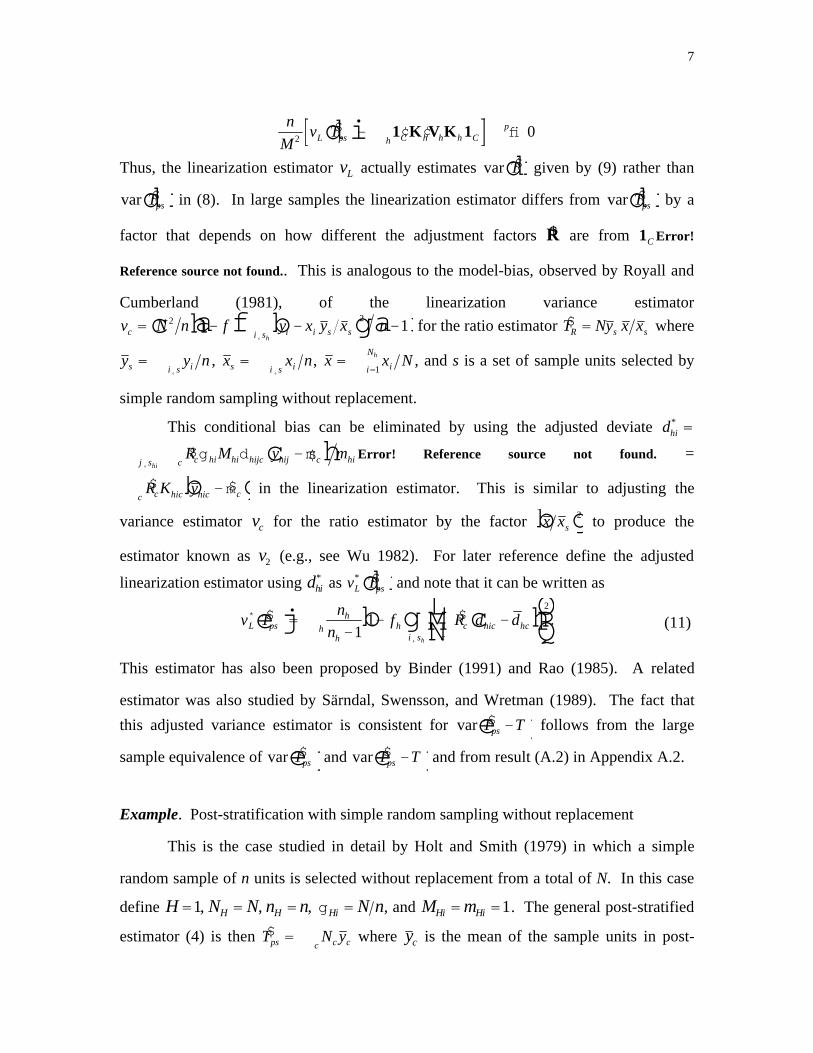
7

n

Mv TL ps C hh h h C

p2

0$d i- ¢ ¢ fi1 K V K 1

Thus, the linearization estimator vL actually estimates var $Tdi given by (9) rather than

var $Tpsdi in (8). In large samples the linearization estimator differs from var $Tpsdi by a

factor that depends on how different the adjustment factors $R are from 1C Error!

Reference source not found.. This is analogous to the model-bias, observed by Royall and

Cumberland (1981), of the linearization variance estimator

v N n f y x y x nc i i s si sh

= - - -˛

2 21 1c ha f b ga f for the ratio estimator $T Ny x xR s s= where

y y ns ii s=

˛, x x ns ii s

=˛

, x x Nii

Nh==1

, and s is a set of sample units selected by

simple random sampling without replacement.

This conditional bias can be eliminated by using the adjusted deviate dhi* =

$ $R M y mc hi hi hijc hij c hicj shi

g d m-˛

c h Error! Reference source not found. =

$ $R K ycc hic hic c-mb g in the linearization estimator. This is similar to adjusting the

variance estimator vc for the ratio estimator by the factor x xsb g2 to produce the

estimator known as v2 (e.g., see Wu 1982). For later reference define the adjusted

linearization estimator using dhi* as v TL ps

* $d i and note that it can be written as

v Tn

nf R d dL ps

h

hh h c hic hc

ci sh

*

˛

=-

- -LNM

OQP

$ $ .ej b g c h1

12

(11)

This estimator has also been proposed by Binder (1991) and Rao (1985). A related

estimator was also studied by Särndal, Swensson, and Wretman (1989). The fact that

this adjusted variance estimator is consistent for var $T Tps -e j follows from the large

sample equivalence of var $Tpsej and var $T Tps -e j and from result (A.2) in Appendix A.2.

Example. Post-stratification with simple random sampling without replacement

This is the case studied in detail by Holt and Smith (1979) in which a simple

random sample of n units is selected without replacement from a total of N. In this case

define H =1, NH = N, nH = n, gHi = N n, and MHi =mHi =1. The general post-stratified

estimator (4) is then $T N yps cc c= where yc is the mean of the sample units in post-

8

stratum c and Nc = Mc is the number of units in the population in post-stratum c. Under

a model with E yibg=m c and var yi cbg=s 2 Error! Reference source not found. if unit i is in

post-stratum c and with all units uncorrelated, the model variance (8) reduces to

Nc2s c

2 ncc. The linearization estimator (10), becomes

v T N n f n s nL ps c cc$e jd ib g b g b g= - - -2 21 1 1 where sc

2 = yi - ycb g2 nc -1b gi˛sc

and yc is

the sample mean for units in post-stratum c. The sample variance sc2 Error! Bookmark not

defined. is a model-unbiased estimator of s c2, and the general form of the approximate

model-bias of vL is bias v T N n n n nN NL ps c c c cc$e j d i d i b g@ -2 2 2 2 2

s . Note that

nN Nc is the expected sample size in a post-stratum under simple random sampling. If,

by chance, the allocation to post-strata is proportional, i.e. n n N Nc c= , then v TL ps$e jis

model-unbiased but, generally, is not. The adjusted linearization estimator, on the other

hand, is approximately conditionally unbiased since v T N s nL ps c c cc

* @$e j 2 2 if n and nc are

large and f is near 0.

5. A BALANCED REPEATED REPLICATION VARIANCE ESTIMATOR

Balanced repeated replication (BRR) or balanced half-sample variance estimators,

proposed by McCarthy (1969), are often used in complex surveys because of their

generality and the ease with which they can be programmed. Suppose nh = 2 in all

strata. A set of J half-samples is defined by the indicators

Vhia =1 if unit i is in half -sample a

0 if notRST

for i=1,2 and a =1,..., J. Based on the Vhia , define

Vhaaf= 2Vh1a -1

=1 if unit h1 is in half -sample a

-1 if unit h2 is in half -sample a .RST

9

Note also that -Vhaaf= 2Vh2a -1. A set of half-samples is orthogonally balanced if

Vha = Vh

a

a=1

J

a=1

JV ¢ha = 0 ¢h „ ha f with a minimal set of half-samples having

H+1£ J £ H+4. One of the choices of balanced half-sample variance estimators is

v T T T JBRR ps ps ps

J$ $ $e j e jbg= -

=

a

a

2

1(12)

where $ $ $T R Tps cc ca a abg bgbg= with $Rc

abg being the post-stratum c adjustment factor and $Tcaaf

being the estimated post-stratum total based on half-sample a , both of which are defined

explicitly below. Other, asymptotically equivalent choices involving the complement to

each half-sample have been studied by Krewski and Rao (1981) and others, but (12)

appears to be the most popular choice in practice.

In applying the BRR method, practitioners often repeat each step of the estimation

or weighting process, including post-stratification adjustments, for each half-sample.

The intuition behind such repetition is that the variance estimator will then incorporate

all sources of variability. The goal here is the estimation of a conditional variance. This

raises the question of whether, to achieve that goal, the post-stratification factors $R

should be recomputed for each half-sample or whether the full-sample factors should be

used for each half-sample.

First, consider the case in which the factors are recomputed from each half-

sample and define $Rcaaf= Mc

$Mcaaf to be the factor and $Tc

aaf to be the estimated total for

post-stratum c based on half-sample a . In particular, $Tcaaf= 2Vhia -1b gKhicyhici˛shh

and $Mcaaf= 2Vhia -1b gKhici˛shh

. Next, expand $Rcaaf$Tc

aaf around the full sample

estimates $Rc and $Tc to obtain the approximation

$Rcaaf$Tc

aaf- $Rc$Tc @ $Rc

$Tcaaf- $Tcd i- $Rc

$m c$Mc

aa f- $Mcd i

= $Rc VhaafD yhc - $m cDKhcc h

h(13)

where D yhc =Kh1cyh1c -Kh2cyh2c and DKhc =Kh1c -Kh2c . The variance estimator (12) can

then be approximated as vBRR$Tpsdi@ $Rc Vh

aafzhchca=1

J2 where zhc = D yhc - $m cDKhc.

10

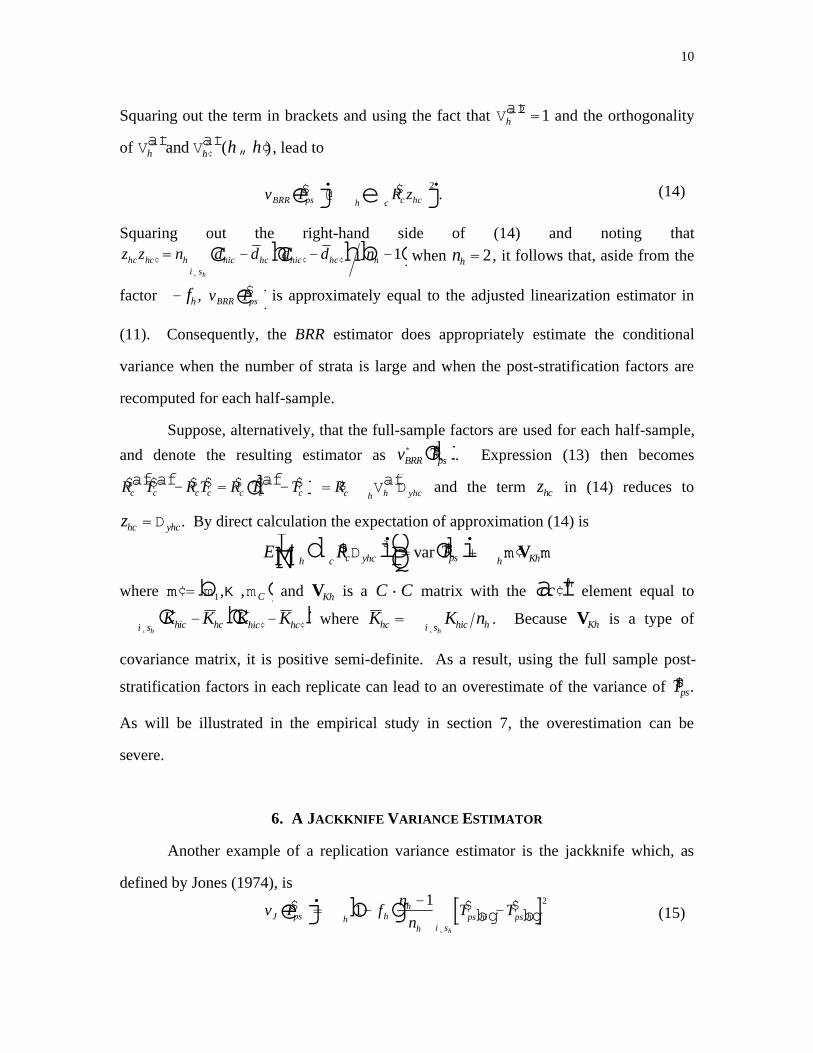
Squaring out the term in brackets and using the fact that Vhaaf2 =1 and the orthogonality

of Vhaaf and V ¢h

aaf (h „ ¢h ) , lead to

v T R zBRR ps c hcch$ $ .ej e j@

2 (14)

Squaring out the right-hand side of (14) and noting thatz z n d d d d nhc hc h hic hc

i shic hc h

h

¢˛

¢ ¢= - - -c hc hb g1 when nh = 2, it follows that, aside from the

factor - fh , v TBRR ps$e j is approximately equal to the adjusted linearization estimator in

(11). Consequently, the BRR estimator does appropriately estimate the conditional

variance when the number of strata is large and when the post-stratification factors are

recomputed for each half-sample.

Suppose, alternatively, that the full-sample factors are used for each half-sample,

and denote the resulting estimator as vBRR* $Tpsdi. Expression (13) then becomes

$ $ $ $ $ $ $R T R T R T Tc c c c c c ca a aafaf afd i- = - = $Rc h yhch

V aafD and the term zhc in (14) reduces to

zhc = D yhc . By direct calculation the expectation of approximation (14) is

E $RcD yhccd i2

hLNM OQP= var $Tpsdi+ ¢mm

hVKhmm

where ¢mm = m1,K ,mCb g and VKh is a C·C matrix with the c ¢cafth element equal to

Khic -Khcc hi˛sh

Khi ¢c -Kh ¢cc h where Khc = Khic nhi˛sh. Because VKh is a type of

covariance matrix, it is positive semi-definite. As a result, using the full sample post-

stratification factors in each replicate can lead to an overestimate of the variance of $Tps.

As will be illustrated in the empirical study in section 7, the overestimation can be

severe.

6. A JACKKNIFE VARIANCE ESTIMATOR

Another example of a replication variance estimator is the jackknife which, as

defined by Jones (1974), is

v T fn

nT TJ ps hh

h

hps hi ps h

i sh

$ $ $e j b g bg bg= --

-˛

11 2

(15)

11

where $Tps hibg is the post-stratified estimator computed after deleting sample cluster (hi)

and $ $T T nps h ps hi hi shaf af=

˛Error! Reference source not found.. Similar to the case of the

BRR estimator, we can write $ $ $T R Tps hi c hic c hibg bg bg= where $ $R M Mc hi c c hibg bg= and $Tc hibg are

estimators derived from deleting sample cluster (hi). Expanding $ $R Tc hi c hibg bg around the full

sample estimates $ $R Tc c and yields$ $ $ $ $ $ $ $ $ $ $ .R T R T R T T R M Mc hi c hi c c c c hi c c c c hi cbg bg bg bge j e j- @ - - -m (16)

For purposes of computation, write the estimated class total as $Tc = Nhh%yhc where

%yhc = %yhic nhi˛sh and %y f K yhic h hic hic= Error! Reference source not found.. Defining

%yhc hiaf= nh %yhc - %yhicc hnh -1b g leads to

$Tc hiaf= Nh %yhc + N ¢h %y ¢h c¢h „h

= $Tc +Nh

nh -1%yhc - %yhicc h

from which it follows that

$Tc hiaf- $Tc haf=-nh

nh -1Khicyhic -

1nh

Kh ¢i cyh ¢i c¢i ˛sh

FHG

IKJ (17)

Similarly, $Mc hiaf- $Mc = -nh Khic - Kh ¢i c¢i ˛she jnh -1b g. Substitution of this expression

and (17) into (16) and use of the resulting approximation in the formula for the jackknife

given by (15) gives

vJ$Tpsdi@ 1- fhb g

h

nh

nh -1$Rc dhic -dhcc h

c

2

i˛sh

å

which is the same as the adjusted linearization variance estimator in (11). Consequently,

by the same arguments presented for v TL ps* $d iError! Reference source not found., the

jackknife estimator is also a consistent estimator of the large sample conditional variance

shown in (8).

7. A SIMULATION STUDY

12

The preceding theory was tested in a simulation study using a fixed, finite

population of 10,841 persons who were included in the September 1988 Current

Population Survey (CPS). The variables used in the study were weekly wages and hours

worked per week for each person. The study population contained 2,826 geographic

segments. The segments were those used in the CPS with each being composed of about

four neighboring households. Eight post-strata were formed on the basis of age, race,

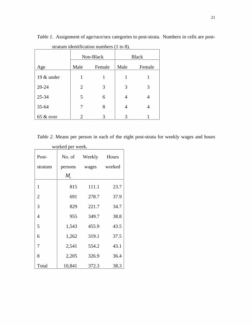
and sex using tabulations of weekly wages on the full population. Table 1 shows the

age/race/sex categories which were assigned to each post-stratum, and Table 2 gives the

means per person of weekly income and hours worked per week in each post-stratum.

As is apparent from Table 2, the means differ considerably among the post-strata,

especially for weekly wages.

A two-stage stratified sample design was used in which segments were selected as

the first-stage units and persons as the second-stage units. Two sets of 10,000 samples

were selected. For the first set, 100 sample segments were selected with probabilities

proportional to the number of persons in each segment. For the second set, 200 segments

were sampled. In both cases, strata were created to have about the same total number of

households and nh = 2 sample segments were selected per stratum. Within each stratum,

segments were selected systematically using the method described by Hansen, Hurwitz,

and Madow (1953, p. 343). A simple random sample of 4 persons was selected without

replacement in each segment having Mhi > 4 . In cases having Mhi £ 4 , all persons in the

sample cluster were selected. For the samples of 100 segments, the first-stage sampling

fraction was 3.5% (100/2826), and for the samples of 200 segments was 7%.

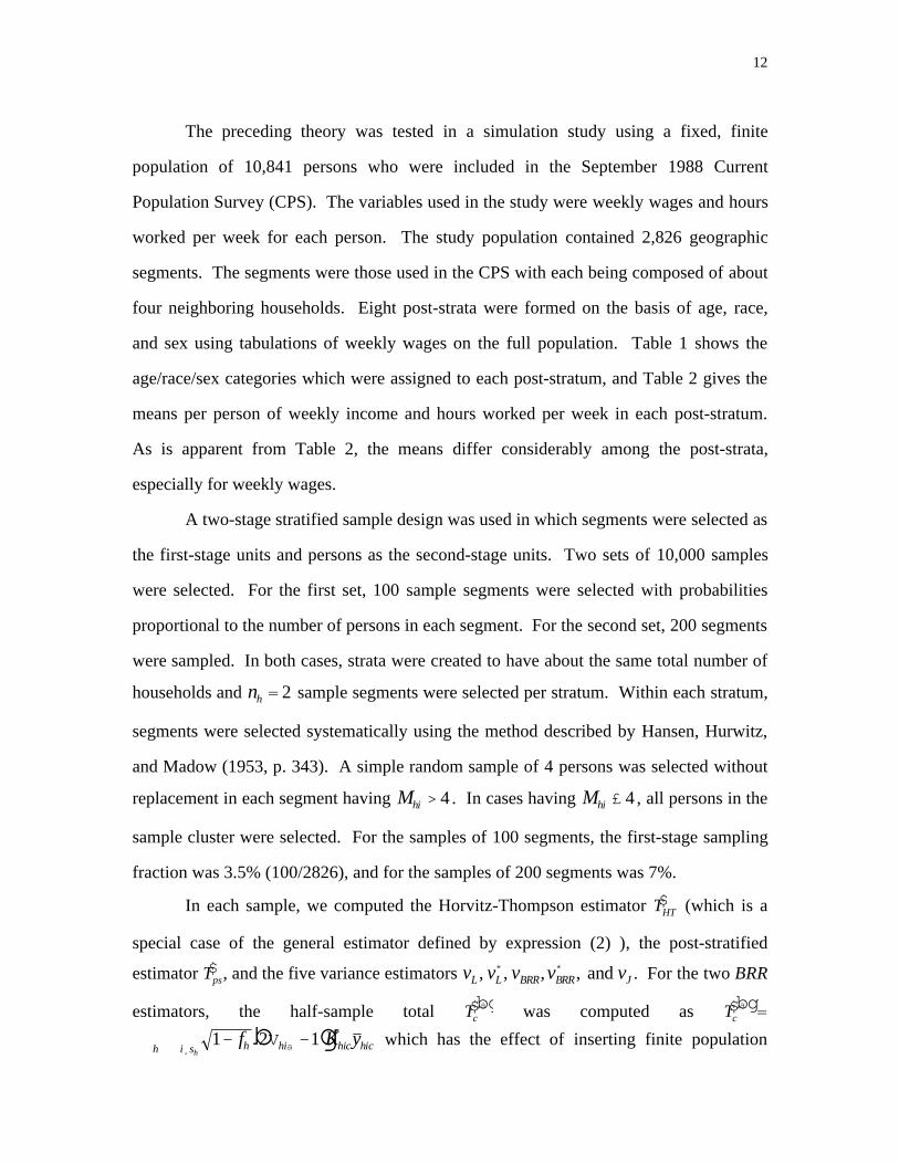
In each sample, we computed the Horvitz-Thompson estimator $THT (which is a

special case of the general estimator defined by expression (2) ), the post-stratified

estimator $Tps, and the five variance estimators vL , vL* , vBRR,vBRR

* , and vJ . For the two BRR

estimators, the half-sample total $Tcabg was computed as $Tc

abg=

1- fhi˛shh2Vhia -1b gKhicyhic which has the effect of inserting finite population

13

correction factors for each stratum in the approximation given by (14). Table 3 presents

unconditional results summarized over all 10,000 samples. Empirical mean square errors

(mse's) were calculated as mse T T T Sss

S$ $ej e j= -=

2

1 with S = 10,000 and $T being either

$THT or $Tps. Average variance estimates across the samples were computed as

v = vs Ss=1

S where vs is one of the five variance estimates considered. The table

reports the ratios v mse T$ej.As anticipated by the theory in section 4 the linearization variance estimator vL is

more nearly an estimate of the mse of the Horvitz-Thompson estimator $THT than of the

mse of $Tps. In fact, the square root of the average vL overestimates the empirical square

root mse Tps$e j from 11% to 17%. The adjusted linearization estimator vL

* , on the other

hand, is approximately unbiased for mse Tps$e j, as is the jackknife. Of the two BRR

estimates, the root of the average vBRR performs well while vBRR* is a serious overestimate

as predicted by the theory in section 5. As the sample increases from n=100 to n=200,

the percentage overestimation by vBRR* drops from 22.9% to 13.3% for wages and from

27.7% to 16.0% for hours. The estimate vBRR* is also much more variable than either vL

*

or vBRR, as shown in the lower part of Table 3. Based on this study, it is clearly

preferable to recompute the post-stratification factors for each half-sample rather than

using the full sample factors each time.

The differences in the performance of the variance estimates may not be nearly so

pronounced in cases where post-stratification does not result in substantial gains over the

Horvitz-Thompson estimator. To illustrate this point, the population was divided into

only two post-strata -- males and females. Another set of 10,000 samples was then

selected for the case n=200. Estimates were made for the variable weekly wages. For

this simulation the empirical square root of the mse of the Horvitz-Thompson estimator

was only 2.9% larger than that of $Tps. This contrasts to the figures in Table 3 for n=200

where the root mse of $THT was 15.7% larger than that of $Tps for weekly wages. The

14

ratios v mse Tps$e j for v v v v vL L BRR BRR J, , , ,* * and were respectively 1.026, .998, .963,

.989, and .998. None of the variance estimates exhibits any substantial deficiencies, and,

in particular, v vL BRR and * estimate mse Tps$e j much more closely than in the eight post-

stratum simulation reported in Table 3.

Figure 1 is a plot that illustrates the conditional empirical biases of the Horvitz-

Thompson and post-stratified estimates for the simulations using eight post-strata. The

bias of $THT under model (1) can be written as E T Rcc cbg- -$ 1 1 where Tc is the

population total for post-stratum c. In the unlikely event that E Tcbg is about the same for

all post-strata, then D = $Rcc

- -1 1e j is proportional to that bias but, more generally, is a

measure of sample balance. D is also a quantity that can be computed for each sample

without knowledge of the expected total in each post-stratum. Samples were sorted in

ascending order by the value of D and were divided into 20 groups of 500 samples each.

The average biases of $THT and $Tps were then computed in each group. The average group

biases for wages and hours are plotted in Figures 1 and 2 versus the average group values

of D. The Horvitz-Thompson estimator has a clear conditional bias even though it is

unbiased over all samples while the conditional bias of the post-stratified estimator is

much less pronounced. When D is extreme, the bias of $THT is also a substantial

proportion of the root mse $THTd i at either sample size for both wages and hours.

The square roots of the average variance estimates within each group are also

plotted as are the empirical square root mse's for each group. The conditional results are

similar to the unconditional ones listed in Table 3. The estimates vL and vBRR* are

substantial overestimates of mse Tps$d iError! Reference source not found. while the other

estimates are approximately unbiased. The estimates vL* , vBRR , and vJ were almost the

same so that, of the three, only vL* is graphed in Figure 1.

The empirical coverage probabilities of 95% confidence intervals were also

computed in the eight post-stratum simulations using $Tps and each of the five variance

15

estimates. The results are what one would expect given the bias characteristics of the

variance estimates and are not shown in detail. The three choices vL* , vBRR , and vJ each

produce intervals with near the nominal coverage probabilities while vBRR* and vL produce

intervals that cover the population total considerably more often than the nominal 95%.

8. CONCLUSION

Post-stratification is an important estimation tool in sample surveys. Though

often thought of as a variance reduction technique, the method also has a role in reducing

the conditional bias of the estimator of a total, as illustrated here. The usual linearization

variance estimator for the post-stratified total $Tps actually estimates an unconditional

variance as shown here both theoretically and empirically. This deficiency is easily

remedied by a simple adjustment which parallels one that can be made for the case of the

ratio estimator. Standard application of the BRR and jackknife variance estimators does,

on the other hand, produce conditionally consistent estimators. An operational question

that is sometimes raised in connection with replication estimators is whether to

recompute the post-stratification factors for each replicate or to use the full sample

factors in each replicate estimate. Judging from the theoretical and empirical results for

BRR reported here, recalculation for each replicate is by far the preferable course,

leading to a variance estimator that is more nearly unbiased and more stable.

An area deserving research, which we have omitted, is the use of post-

stratification to correct for sample nonresponse and for coverage problems in sampling

frames. In the U.S. Current Population Survey, for example, post-stratification leads to

substantial upward adjustments in weights for some demographic groups. For Black

males, for example, the upward adjustments can range from less than 1% to more than

35% depending on age group (U.S. Bureau of the Census 1978).

APPENDIX

16

A.1 Prediction variance of the post-stratified estimator

This appendix sketches the derivation of the prediction variance of the post-

stratified estimator of the total and the identification of the dominant term in the

variance. Large sample calculations will be done for a situation in which Hfi ¥ , all

parameters in model (1) are finite, and in which

(i) n Mfi 0,

(ii) maxh,i

Mhib g, maxh,i

mhib g, maxh

Nhbg and maxh

nhb g are O 1a f,

(iii) maxh,i,c

Khicb g=O M na f(iv) $Rfi R, a constant

(v) n M2c h ¢KhhVhKh fi GG, a C·C positive definite matrix of constants, and

(vi) M-1 E Khic yhic -m cb gh

2+d=O 1af for some d >0 and for all i and c.

Conditions (i) - (iii) are bounding conditions on sample and population sizes. The three

are consistent with surveys having a large number of strata, but with population and

sample sizes in any stratum being restricted. Condition (iv) requires that each post-

stratum factor $Rc converge to a constant, which is not necessarily 1, as Hfi ¥ .

Condition (v) requires the covariance matrix of $T1,K , $TCd i to have a limit when

multiplied by the normalizing factor n M2 . Finally, (vi) is a standard Liapounov

condition on moments of Khicyhic. Next, consider the prediction error of $Tps which is

$Tps -T = $Rc

Khic

mhic

-1LNM

OQP

jshiishch yhijdhijc

- yhijdhijcjshiish

ch - yhijdhijcj=1

Mhi

ishch

= A- B-C

where A, B, and C are defined by the last equality. Using this decomposition, the

prediction variance under model (1) is

var $Tps -Td i= var Aaf+var Baf+var Ca f - 2cov A, Ba f.

17

First, examine var(A) and define Lhic = $RcKhic mhic -1d imhic . From assumptions (i) - (iii)

above, Error! Reference source not found. and under the model for the means yhic given by

(5), we have

var Aaf= Lhic2 vhicc

+ LhicLhi ¢c thic ¢c¢c „cco t

i shh

» ¢Rh

¢K hV hK hR .

From (iv) and (v) var Aaf=O M2 nc h.In order to compute the other components of the variance, some additional

notation will be used. Define v1hic =s hic2 1+ Mhic -mhic -1b grhic and

v2hic = s hic2 1+ Mhic -1b grhic . The other components of the prediction variance under

model (1) and their orders of magnitude are then obtained by direct computation as

var Baf= Mhic -mhicb gi˛sh

v1hic + M hi ¢c - m hi ¢cb g t hic ¢c¢c ¹ c

å

R

ST

U

VW

cåhå

= O na f f r o m ( i i ) ,

var Caf= Mhiciˇsh

v2hic + MhicMhi ¢c thic¢c¢c„c

RST

UVW

ch

=O N -na ffrom (ii),and

cov A, Ba f= $RcchKhicmhici˛sh

å Mh ic

- mh ic

b g sh ic

2r

h ic+ M

h i ¢c- m

h i ¢cb g t

h ic ¢c

¢c ¹ c

å

R

S

T

U

V

W

= O Ma f f r o m ( i i ) , ( i i i ) , a n d ( i v ) ,

Pursuant to these calculations and (i), the dominant term of the prediction variance is

var Aaf and it is easy to show that var Aaf» var $Tpsdi.

A.2 Other large sample properties

The conditions listed in section A.1 are also sufficient to derive the large sample

distribution of the post-stratified estimator and a property of one of the quantities

18

associated with each of the variance estimators considered in the earlier sections. Two

key results are that as Hfi ¥ , if conditions (ii), (iii), (v), and (vi) hold, then

(1)n

M$T1 -m1 Khi1,K , $TC -mC KhiC

iÎshåhå

iÎshåhå

F

HGI

KJd¾ ®¾ N 0,Ga f , and (A.1)

(2)n

M2 v $Thej- ¢KhVhKhhh

pfi 0 (A.2)

where v $Thej is a C·C matrix whose c ¢cafth element is

v $Thejc ¢c=

nh

nh -1dhic- dhcc h

iÎshå dhi ¢c - dh¢cc h

with dhic = Khic yhic - $m cb g and dhc = dhic nhi˛sh. These results can be proved using

Lemmas 3.1 and 3.2, given in Krewski and Rao (1981), which are a central limit theorem

and a law of large numbers for independent, nonidentically distributed random variables.

Details of the proofs are lengthy but routine and, for brevity, are not presented here. As

an immediate consequence of (A.1), (A.2), and (iv) from section A.1, we have

$Tps -Td i$¢R v $The j $Rhå

d¾ ®¾ N 0,1a f

so that the usual normal theory confidence intervals are justified.

REFERENCES

Binder, D. (in press), "Use of Estimating Equations for Interval Estimation from

Complex Surveys," 1991 Proceedings of the Section on Survey Research

Methods, American Statistical Association.

Durbin, J. (1969), "Inferential Aspects of the Randomness of Sample Size in Survey

Sampling," in New Developments in Survey Sampling, N.L. Johnson and H.

Smith, Jr. eds, Wiley-Interscience, 629-651.

19

Hansen, M.H., Hurwitz, W., and Madow, W. (1953), Sample Survey Methods and

Theory (Vol. 1), New York: John Wiley.

Holt, D. and Smith, T.M.F. (1979), "Post Stratification," Journal of the Royal Statistical

Society A, 142, 33-46.

Jones, H.L. (1974), "Jackknife Estimation of Functions of Stratum Means," Biometrika,

61, 343-348.

Krewski, D. and Rao, J.N.K. (1981), "Inference from Stratified Samples: Properties of

the Linearization, Jackknife, and Balanced Repeated Replication Methods,"

Annals of Statistics, 9, 1010-1019.

McCarthy, P.J. (1969), "Pseudo-replication: Half-Samples," Review of the International

Statistical Institute, 37, 239-264.

Parsons, V.L. and Casady, R.J. (1985), "Variance Estimation and the Redesigned

National Health Interview Survey, Proceedings of the Section on Survey Research

Methodology, American Statistical Association, 406-411.

Rao, J.N.K. (1985), "Conditional Inference in Survey Sampling," Survey Methodology,

11, 15-31.

Royall, R.M. (1986), "The Prediction Approach to Robust Variance Estimation in Two-

Stage Cluster Sampling," Journal of the American Statistical Association, 81,

119-123.

Royall, R.M. and Cumberland, W.G. (1981), "An Empirical Study of the Ratio Estimator

and Estimators of its Variance," Journal of the American Statistical Association,

76, 66-77.

Särndal, C.-E., Swensson, B., and Wretman, J. (1989), "The Weighted Residual

Technique for the Estimating the Variance of the General Regression Estimator

of the Finite Population Total," Biometrika, 76, 527-537.

U.S. Bureau of the Census (1978), The Current Population Survey: Design and

Methodology, Technical Paper 40, Dept. of Commerce: Washington DC.

20

Valliant, R. (1987), "Generalized Variance Functions in Stratified Two-Stage Sampling,"

Journal of the American Statistical Association, 82, 499-508.

Williams, W.H. (1962), "The Variance of an Estimator with Post-Stratified Weighting,"

Journal of the American Statistical Association, 57, 622-627.

Wu, C.F.J. (1982), "Estimation of the Variance of the Ratio Estimator," Biometrika, 69,

183-189.

FIGURE TITLES

Figure 1. Conditional bias, root mean squared error, and standard error estimates for

weekly wages in the simulation using eight post-strata. Two sets of 10,000 two-stage

stratified samples were selected. Samples were sorted on a measure of sample balance

and divided into 20 groups of 500 samples each in order to compute conditional

properties.

Figure 2. Conditional bias, root mean squared error, and standard error estimates for

hours worked per week in the simulation using eight post-strata. Two sets of 10,000

two-stage stratified samples were selected. Samples were sorted on a measure of sample

balance and divided into 20 groups of 500 samples each in order to compute conditional

properties.

21

Table 1. Assignment of age/race/sex categories to post-strata. Numbers in cells are post-

stratum identification numbers (1 to 8).

Non-Black Black

Age Male Female Male Female

19 & under 1 1 1 1

20-24 2 3 3 3

25-34 5 6 4 4

35-64 7 8 4 4

65 & over 2 3 3 1

Table 2. Means per person in each of the eight post-strata for weekly wages and hours

worked per week.

Post-

stratum

No. of

persons

Mc

Weekly

wages

Hours

worked

1 815 111.1 23.7

2 691 278.7 37.9

3 829 221.7 34.7

4 955 349.7 38.8

5 1,543 455.9 43.5

6 1,262 319.1 37.5

7 2,541 554.2 43.1

8 2,205 326.9 36.4

Total 10,841 372.3 38.3

22

Table 3. Unconditional summary results over two sets of 10,000 two-stage stratified

samples of 100 and 200 segments each. Eight post-strata, defined in Table 1 were used.

Weekly wages Hours worked

Summary quantity n=100 n=200 n=100 n=200

Empirical mse ‚103c h $THT 156.1 111.1 6.8 4.9

$Tps 138.0 96.0 6.2 4.3

vL mse $THTd i 1.034 1.002 1.031 .993

[Avg. var. est./mse $Tpsdi]1/2

vL 1.170 1.159 1.122 1.110

vL*

1.004 1.013 .999 .998

vBRR 1.061 .993 1.028 .982

vBRR*

1.229 1.133 1.277 1.160

vJ 1.006 1.014 1.002 .998

Std. dev. of var. est.(‚106 )

vL 5616 1935 14.7 5.1

vL*

4290 1500 12.2 4.2

vBRR 4941 1455 13.1 4.1

vBRR*

6900 2022 20.9 6.2

vJ 4326 1503 12.3 4.2