Embed Size (px)
Citation preview

Philippe O. A. Navaux [email protected]
2nd Workshop of the HPC-GA project
Porting Ondes 3D to Adaptive MPI
Informatics Institute, Federal University of
Rio Grande do Sul, Brazil
Parallel and DistributedProcessing Group
Rafael Keller [email protected]
Víctor Martí[email protected]
Outline
1. Introduction
2. Charm++ and AMPI
3. Port of Ondes3D to MPI
4. Evaluation
5. Final Considerations

3
1. Introduction1. Introduction
4
1.1 Ondes 3D
• Ondes3D: Simulator of three-dimensional seismical wave propagation;
• Problem description: – Needs artificial boundary conditions to absorb the energy
that goes out of the simulated region;
• this results in different loads between the regions that compose the simulated domain;
• especially in the inferior and lateral borders.
• Suggestion:– Load balancing with Charm++;
• based on process migration.
5
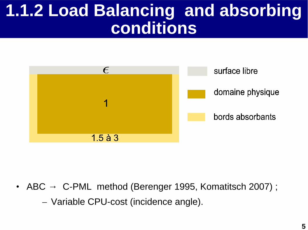
1.1.2 Load Balancing and absorbing conditions
• ABC → C-PML method (Berenger 1995, Komatitsch 2007) ;
– Variable CPU-cost (incidence angle).
6
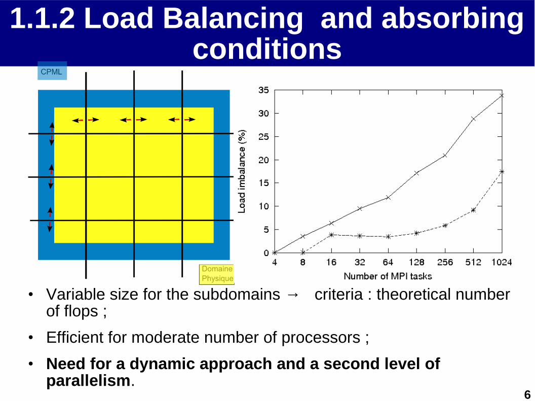
1.1.2 Load Balancing and absorbing conditions
• Variable size for the subdomains → criteria : theoretical number of flops ;
• Efficient for moderate number of processors ;
• Need for a dynamic approach and a second level of parallelism.
7
1.2 Port of Ondes3D to AMPI
• First step towards a possible port to Charm++:– Port of an MPI implementation of Ondes 3D to
AMPI;
• AMPI: Adaptive MPI– MPI implementation built upon the same foundation
as Charm++;

8
2. Charm++ and AMPI2. Charm++ and AMPI
9
2.1 Charm++
• Charm++:– machine independent parallel programming
system;
– programs run unchanged on MIMD machines with or without a shared memory;
– Suport for dynamic and static load balancing;
• Charm++ programs are written in C++;
10
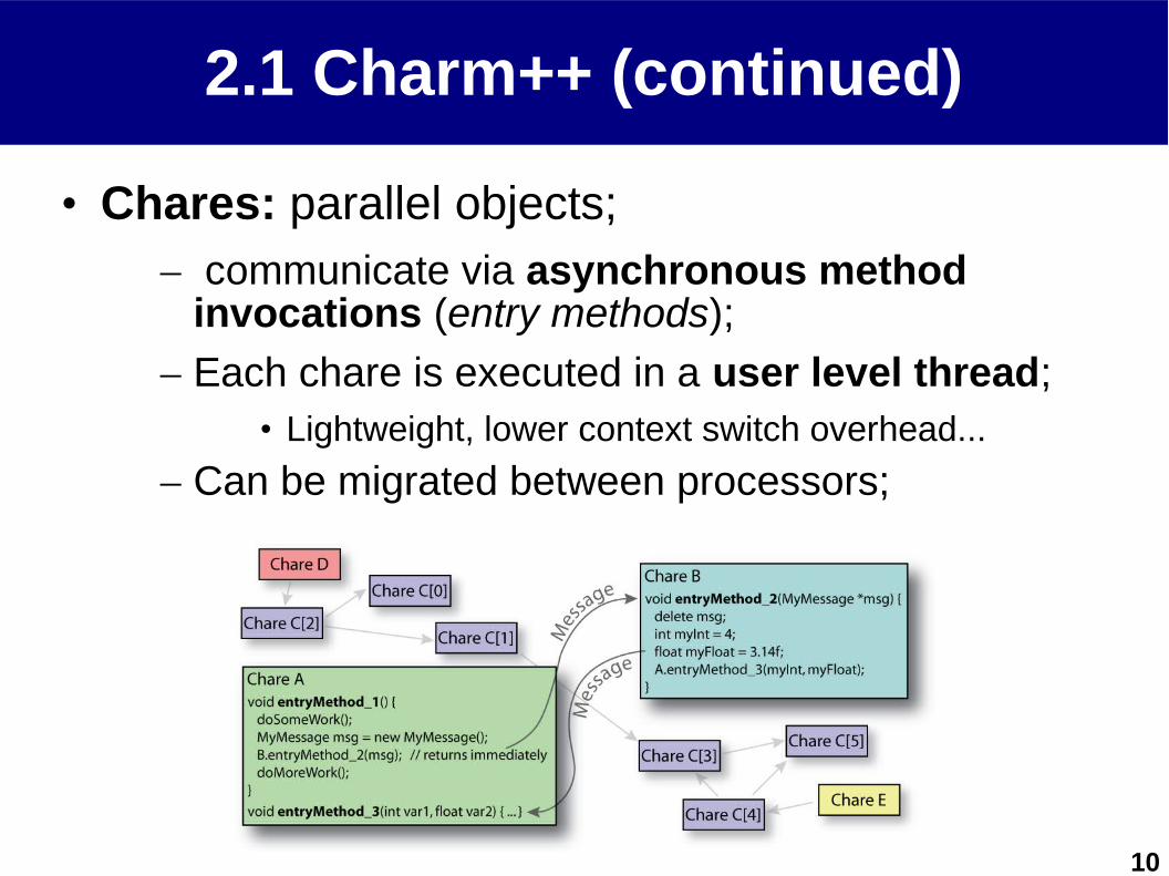
2.1 Charm++ (continued)
• Chares: parallel objects;– communicate via asynchronous method
invocations (entry methods);
– Each chare is executed in a user level thread;• Lightweight, lower context switch overhead...
– Can be migrated between processors;
11
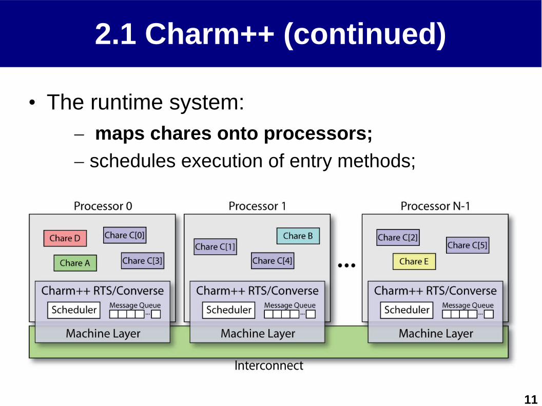
2.1 Charm++ (continued)
• The runtime system:– maps chares onto processors;
– schedules execution of entry methods;
12
2.1 Charm++ (continued)
• Dynamic Load Balancing:– The runtime collects data about the execution of
the program;
– A load balancer uses this data to decide which processes need to be migrated;
– Migrate chares between processes in order to achieve a better ditribution of the load;
– Support for several load-balancing strategies;
– The user can write his own custom load-balancer;

13
2.2 AMPI: Adaptive MPI
• MPI implementation;– Built upon the same foundation as Charm++;
14
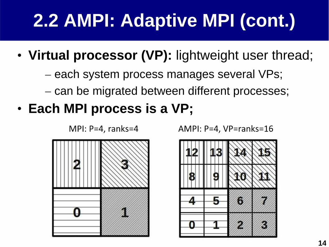
2.2 AMPI: Adaptive MPI (cont.)
• Virtual processor (VP): lightweight user thread;– each system process manages several VPs;
– can be migrated between different processes;
• Each MPI process is a VP;
15
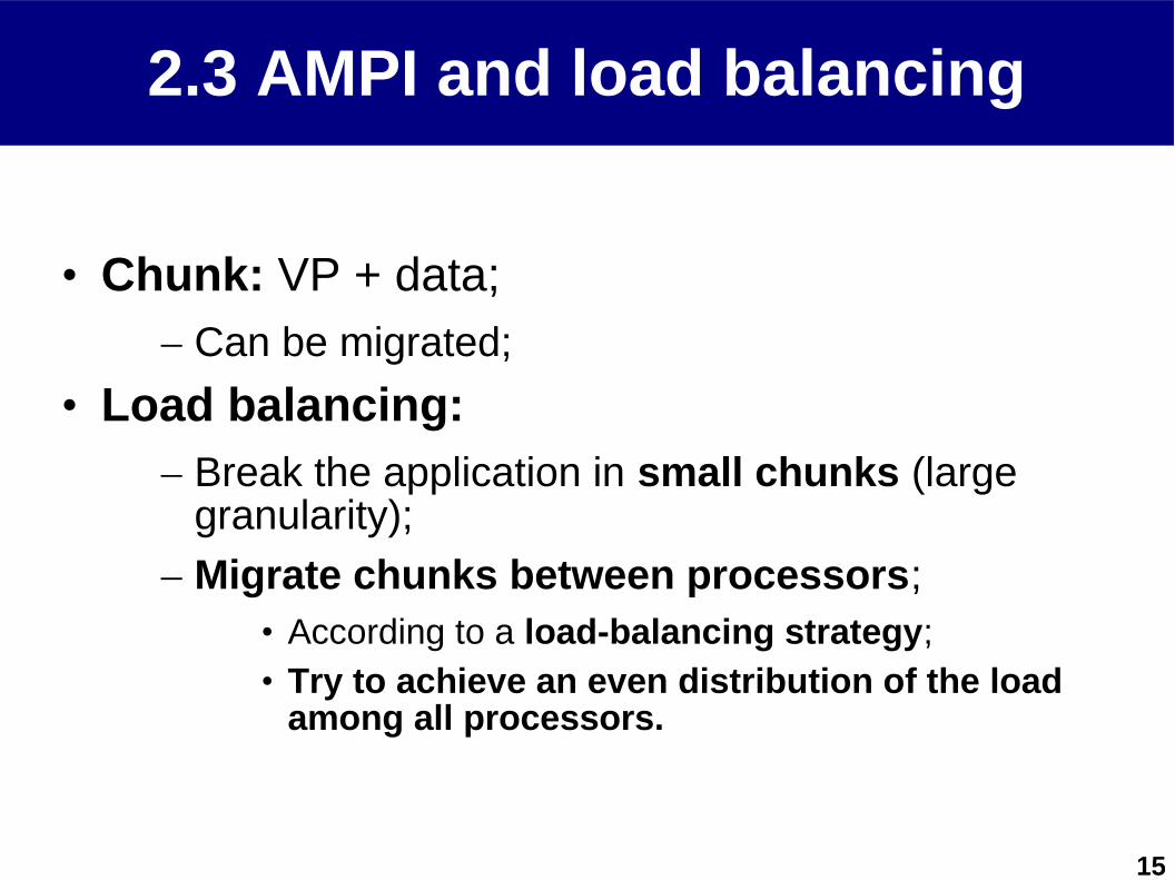
2.3 AMPI and load balancing
• Chunk: VP + data;– Can be migrated;
• Load balancing:– Break the application in small chunks (large
granularity);
– Migrate chunks between processors;• According to a load-balancing strategy;• Try to achieve an even distribution of the load
among all processors.
16
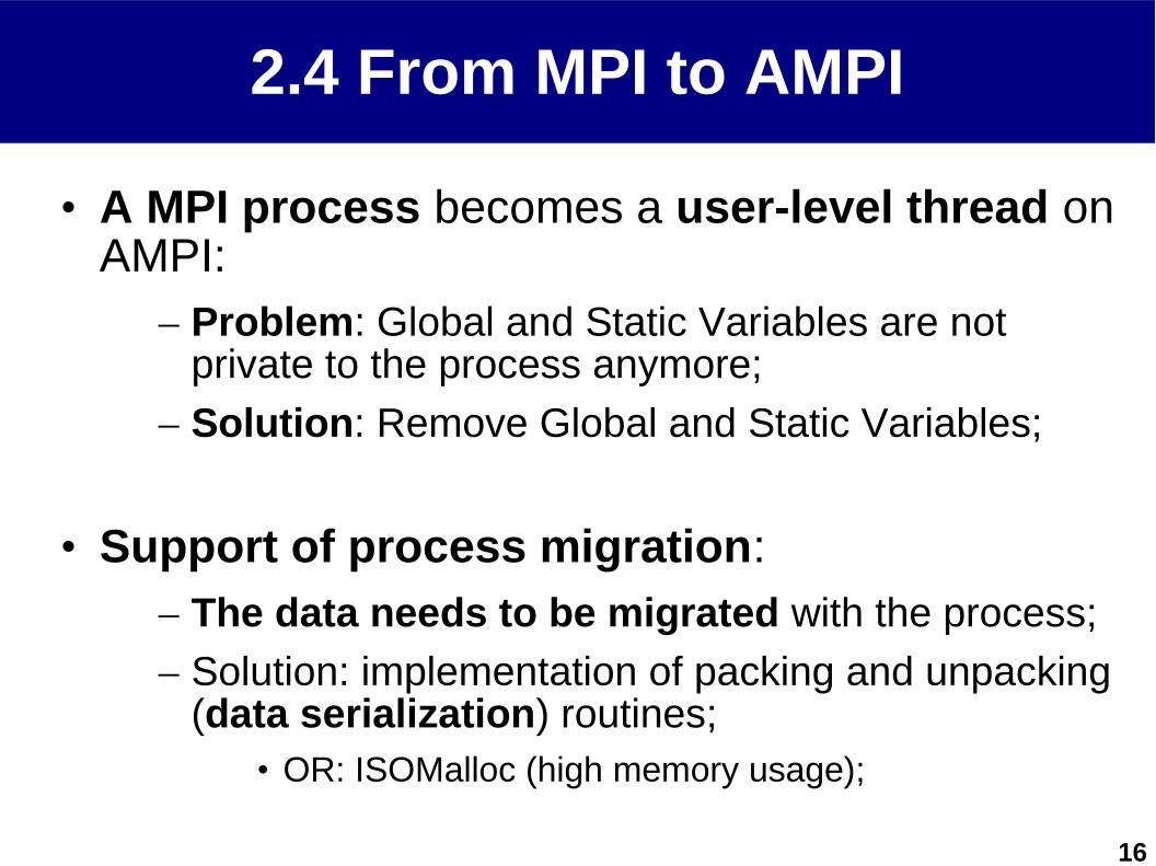
2.4 From MPI to AMPI
• A MPI process becomes a user-level thread on AMPI:
– Problem: Global and Static Variables are not private to the process anymore;
– Solution: Remove Global and Static Variables;
• Support of process migration:– The data needs to be migrated with the process;
– Solution: implementation of packing and unpacking (data serialization) routines;
• OR: ISOMalloc (high memory usage);
17
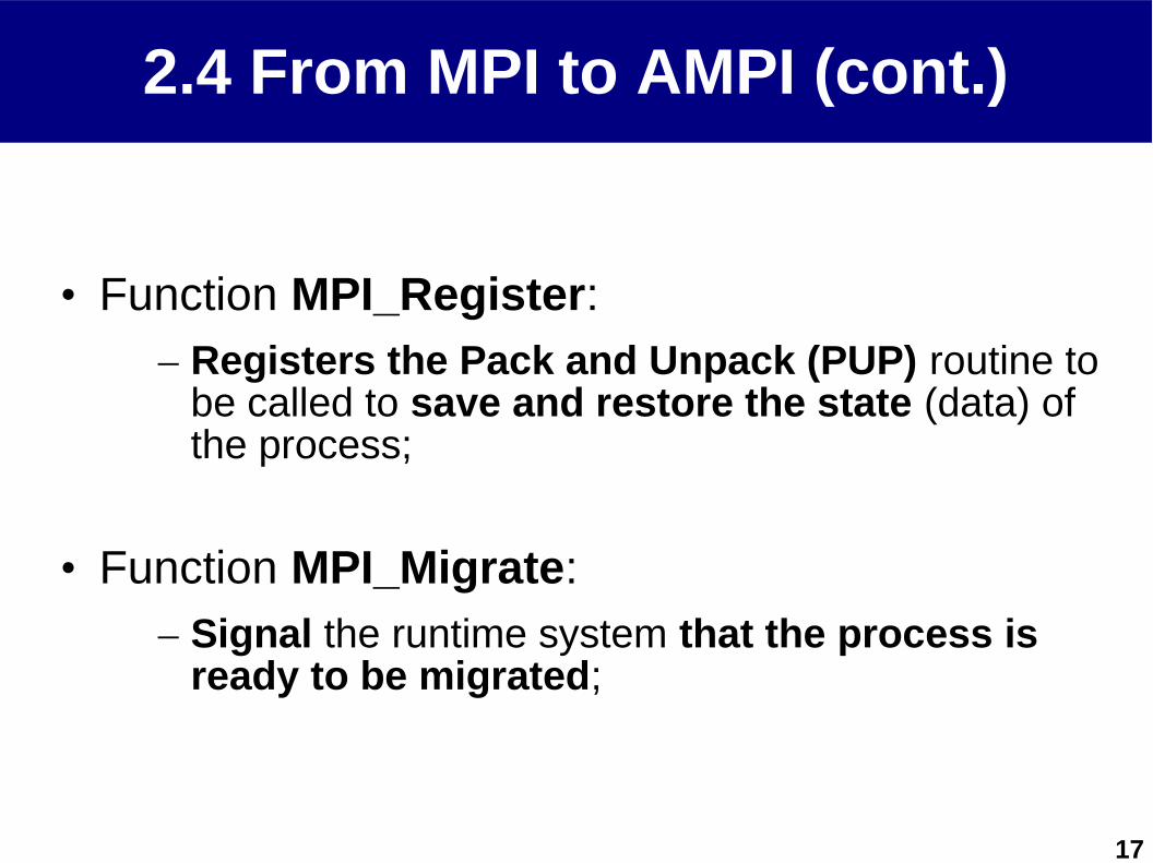
2.4 From MPI to AMPI (cont.)
• Function MPI_Register:– Registers the Pack and Unpack (PUP) routine to
be called to save and restore the state (data) of the process;
• Function MPI_Migrate:– Signal the runtime system that the process is
ready to be migrated;

18
2.5 Pack and Unpack Routines
• The migration process can be broken in three main steps;
– Pack the data belonging to the process (before migration);
– Migrate the process to the new processor;
– Unpack the data in order to restore the current state of the process.
19
2.5 Pack and unpack routines (cont.)
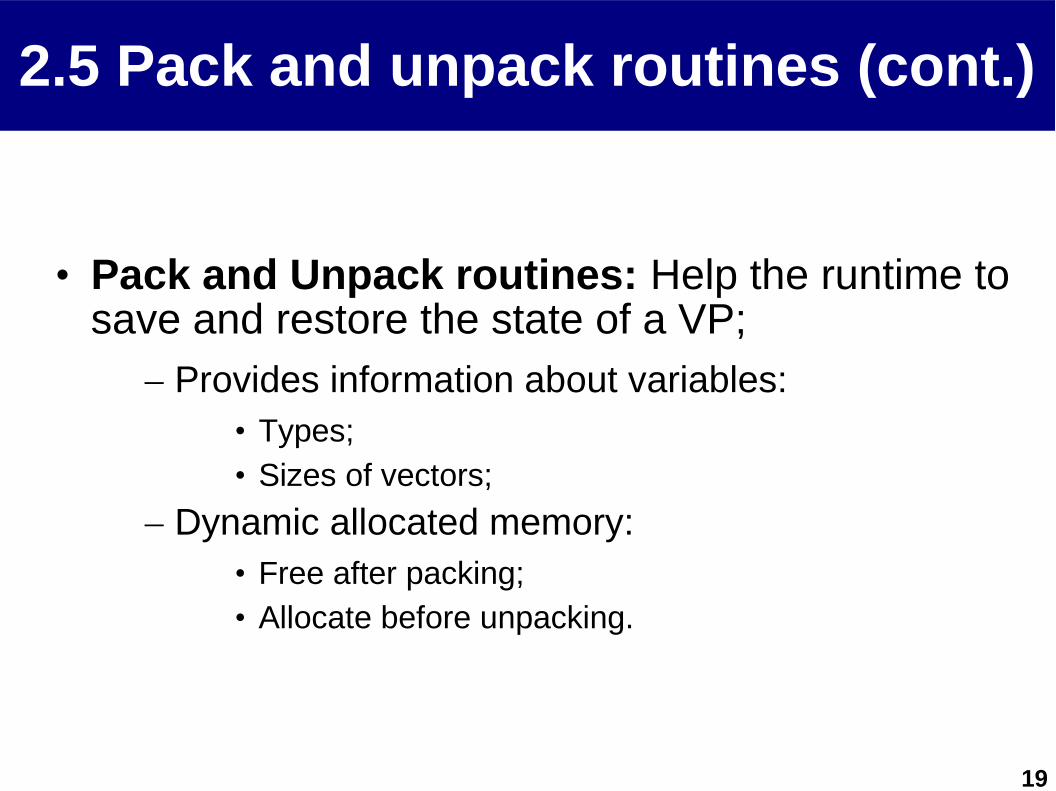
• Pack and Unpack routines: Help the runtime to save and restore the state of a VP;
– Provides information about variables:• Types;• Sizes of vectors;
– Dynamic allocated memory:• Free after packing;• Allocate before unpacking.

20
3. Port of Ondes3D to AMPI3. Port of Ondes3D to AMPI
21
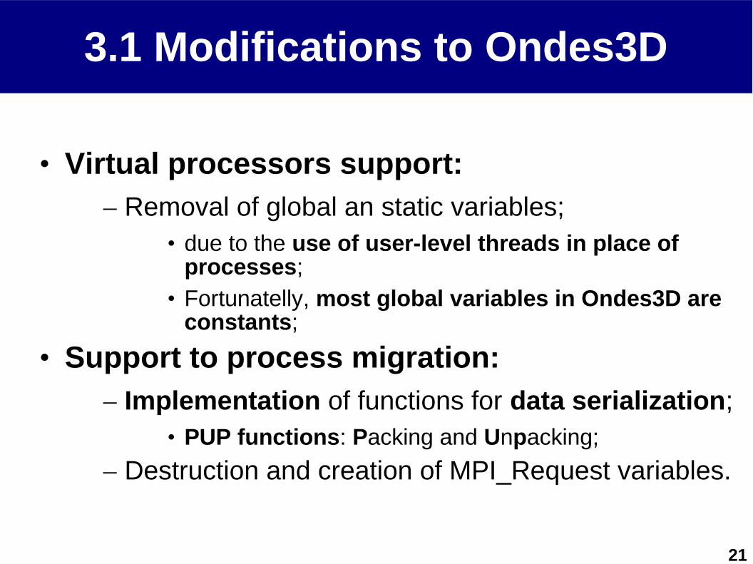
3.1 Modifications to Ondes3D
• Virtual processors support:– Removal of global an static variables;
• due to the use of user-level threads in place of processes;
• Fortunatelly, most global variables in Ondes3D are constants;
• Support to process migration:– Implementation of functions for data serialization;
• PUP functions: Packing and Unpacking;
– Destruction and creation of MPI_Request variables.

22
3.1.2 Removal of global and static variables from Ondes3D (example)
/*From “nrutil.h” (MPI) */
static float sqrarg;#define SQR(a) ((sqrarg=(a)) == 0.0 ? 0.0 : sqrarg*sqrarg)
static double dsqrarg;#define DSQR(a) ((dsqrarg=(a)) == 0.0 ? 0.0 : dsqrarg*dsqrarg)
static double dmaxarg1,dmaxarg2;#define DMAX(a,b) (dmaxarg1=(a),dmaxarg2=(b),(dmaxarg1) > (dmaxarg2) ?\ (dmaxarg1) : (dmaxarg2))
/*From “nrutil.h” (AMPI)*/
#define SQR(a) (a==0.0?0.0:(float)a*(float)a)
#define DSQR(a) (a==0.0?0.0:(double)a*(double)a)
#define MAX_VAL(a,b)((a) > (b) ? (a) : (b))#define DMAX(a,b) MAX_VAL((double)a,(double)b)
/* In the MPI code many constants were declared as * global variables. */
/* From “main.c” (MPI)*/
#ifndef TOPOLOGIEstatic const char TOPOFILE[50]= "topologie.in";#elsestatic const char TOPOFILE[50]= QUOTEME(TOPOLOGIE);#endif
/* Those were replaced by using the command #define * of the C preprocessor. */
/* From “main.c” (AMPI) */
#ifndef TOPOLOGIE#define TOPOFILE "topologie.in"#else#define TOPOFILE QUOTEME(TOPOLOGIE)#endif
23
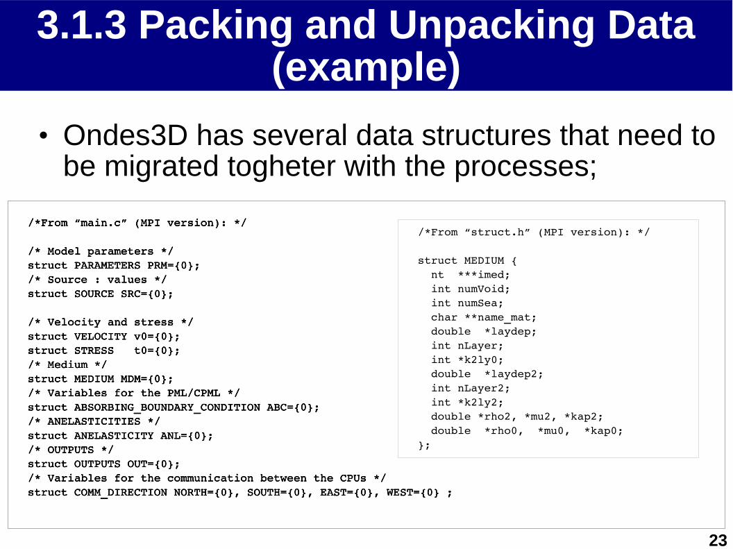
3.1.3 Packing and Unpacking Data (example)
• Ondes3D has several data structures that need to be migrated togheter with the processes;
/*From “main.c” (MPI version): */
/* Model parameters */struct PARAMETERS PRM={0};/* Source : values */struct SOURCE SRC={0};
/* Velocity and stress */struct VELOCITY v0={0};struct STRESS t0={0};/* Medium */struct MEDIUM MDM={0};/* Variables for the PML/CPML */struct ABSORBING_BOUNDARY_CONDITION ABC={0};/* ANELASTICITIES */struct ANELASTICITY ANL={0};/* OUTPUTS */struct OUTPUTS OUT={0};/* Variables for the communication between the CPUs */struct COMM_DIRECTION NORTH={0}, SOUTH={0}, EAST={0}, WEST={0} ;
/*From “struct.h” (MPI version): */
struct MEDIUM { nt ***imed; int numVoid; int numSea; char **name_mat; double *laydep; int nLayer; int *k2ly0; double *laydep2; int nLayer2; int *k2ly2; double *rho2, *mu2, *kap2; double *rho0, *mu0, *kap0;};
/*From “main.c” (MPI version): */
/* Model parameters */struct PARAMETERS PRM={0};/* Source : values */struct SOURCE SRC={0};
/* Velocity and stress */struct VELOCITY v0={0};struct STRESS t0={0};/* Medium */struct MEDIUM MDM={0};/* Variables for the PML/CPML */struct ABSORBING_BOUNDARY_CONDITION ABC={0};/* ANELASTICITIES */struct ANELASTICITY ANL={0};/* OUTPUTS */struct OUTPUTS OUT={0};/* Variables for the communication between the CPUs */struct COMM_DIRECTION NORTH={0}, SOUTH={0}, EAST={0}, WEST={0} ;

24
3.1.3 Packing and Unpacking Data (example)
Fragment of the: PUP function for struct MEDIUM:
/*From “pup.c” (AMPI version):*/
/* A fragment of the code tha serializes a variable of type ().*/pup_medium(pup_er p, struct MEDIUM *MDM, struct PARAMETERS *PRM){ int i; pup_int(p, &(MDM>nLayer)); pup_int(p, &(MDM>nLayer2)); if(model == GEOLOGICAL){ if(pup_isUnpacking(p)){//We need to allocate memory for dynamic variables. MDM>name_mat = calloc(MDM>nLayer, sizeof(char*)); for (i = 0 ; i < MDM>nLayer; i++){ MDM>name_mat[i] = calloc(STRL, sizeof (char)); } } pup_i3tensor(p, &MDM>imed, 1, PRM>mpmx + 2, 1, PRM>mpmy + 2, PRM>zMinPRM>delta, PRM>zMax0); pup_int(p, &(MDM>numVoid)); pup_int(p, &(MDM>numSea)); for (i = 0 ; i < MDM>nLayer; i++){ pup_chars(p, MDM>name_mat[i], STRL); }
...

25
3.1.3 Packing and Unpacking Data (example)
Another example of PUP Function:
/*From “pup.c” (AMPI version):*/void pup_i3tensor(pup_er p, int ****i3t, int x_start, int x_end, int y_start, int y_end, int z_start, int z_end){ if(pup_isUnpacking(p)){ *i3t = i3tensor(x_start, x_end, y_start, y_end, z_start, z_end); } int *real_start = (*i3t)[x_start][y_start] + z_start; int dim_x = x_end x_start + 1; int dim_y = y_end y_start + 1; int dim_z = z_end z_start + 1; pup_ints(p, real_start, dim_x * dim_y * dim_z); if(pup_isPacking(p)){ free_i3tensor(*i3t, x_start, x_end, y_start, y_end, z_start, z_end); }}
...
26
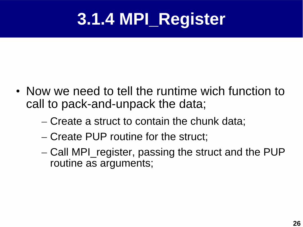
3.1.4 MPI_Register
• Now we need to tell the runtime wich function to call to pack-and-unpack the data;
– Create a struct to contain the chunk data;
– Create PUP routine for the struct;
– Call MPI_register, passing the struct and the PUP routine as arguments;
27
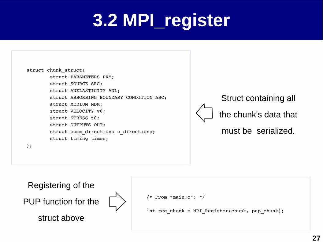
3.2 MPI_register
struct chunk_struct{ struct PARAMETERS PRM; struct SOURCE SRC; struct ANELASTICITY ANL; struct ABSORBING_BOUNDARY_CONDITION ABC; struct MEDIUM MDM; struct VELOCITY v0; struct STRESS t0; struct OUTPUTS OUT; struct comm_directions c_directions; struct timing times;};
/* From “main.c”: */
int reg_chunk = MPI_Register(chunk, pup_chunk);
Struct containing all
the chunk's data that
must be serialized.
Registering of the
PUP function for the
struct above

28
3.3 MPI_Migrate
/* From “main.c”: */
#ifndef MIGRATION_STEP#define MIGRATION_STEP 20#endif
//...
//At the end of the main loop: if(((l % MIGRATION_STEP) == 0) && (l < PRM>tMax)){ MPI_Migrate(); }//...
• Last, we need to tell the runtime when the process is ready to be migrated:

29
4. Evaluation4. Evaluation
30
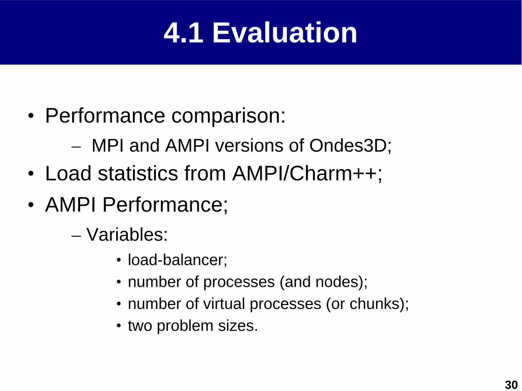
4.1 Evaluation
• Performance comparison:– MPI and AMPI versions of Ondes3D;
• Load statistics from AMPI/Charm++;
• AMPI Performance;– Variables:
• load-balancer;• number of processes (and nodes);• number of virtual processes (or chunks);• two problem sizes.
31
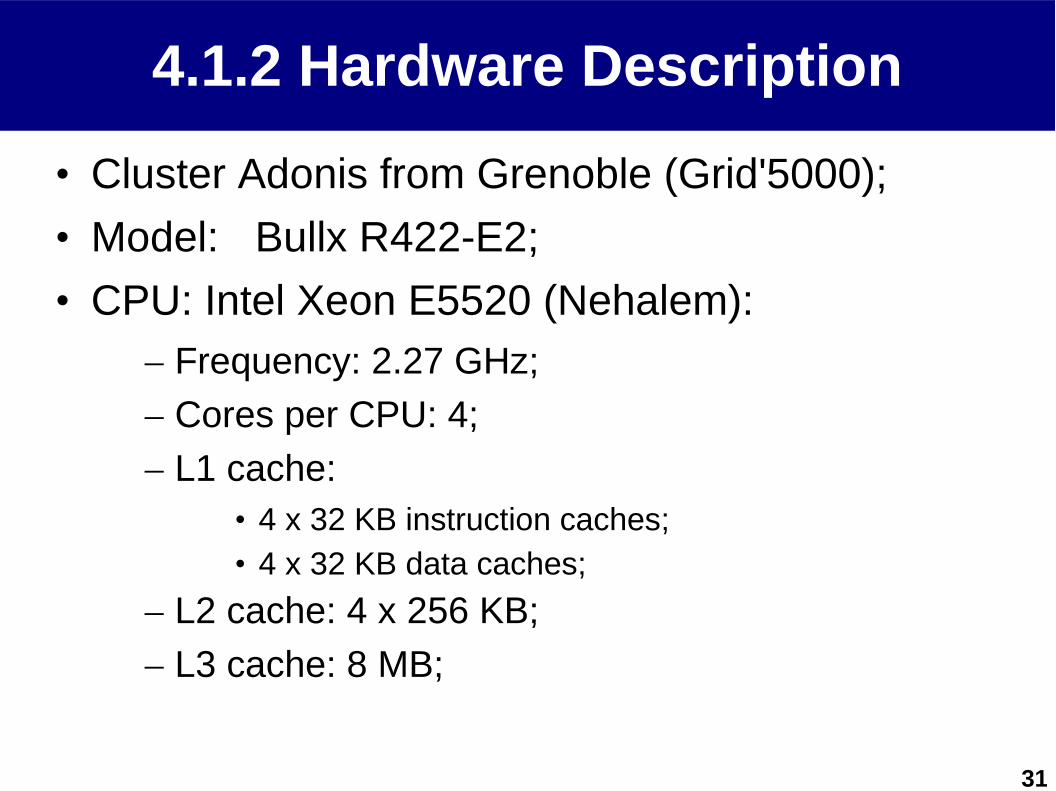
4.1.2 Hardware Description
• Cluster Adonis from Grenoble (Grid'5000);
• Model: Bullx R422-E2;
• CPU: Intel Xeon E5520 (Nehalem):– Frequency: 2.27 GHz;
– Cores per CPU: 4;
– L1 cache:• 4 x 32 KB instruction caches;• 4 x 32 KB data caches;
– L2 cache: 4 x 256 KB;
– L3 cache: 8 MB;
32
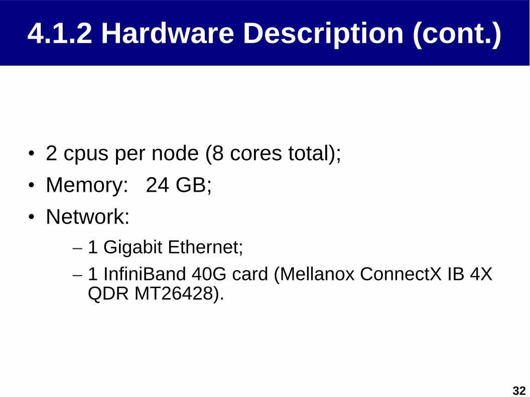
4.1.2 Hardware Description (cont.)
• 2 cpus per node (8 cores total);
• Memory: 24 GB;
• Network:– 1 Gigabit Ethernet;
– 1 InfiniBand 40G card (Mellanox ConnectX IB 4X QDR MT26428).
33
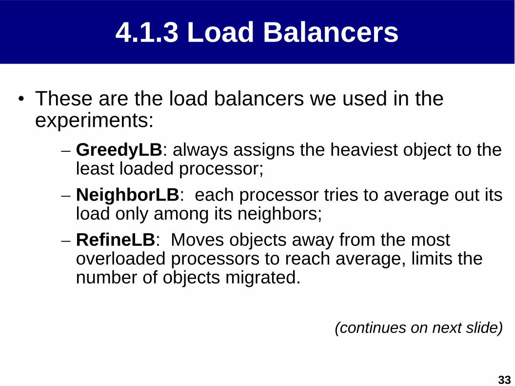
4.1.3 Load Balancers
• These are the load balancers we used in the experiments:
– GreedyLB: always assigns the heaviest object to the least loaded processor;
– NeighborLB: each processor tries to average out its load only among its neighbors;
– RefineLB: Moves objects away from the most overloaded processors to reach average, limits the number of objects migrated.
(continues on next slide)
34
4.1.3 Load Balancers (cont.)
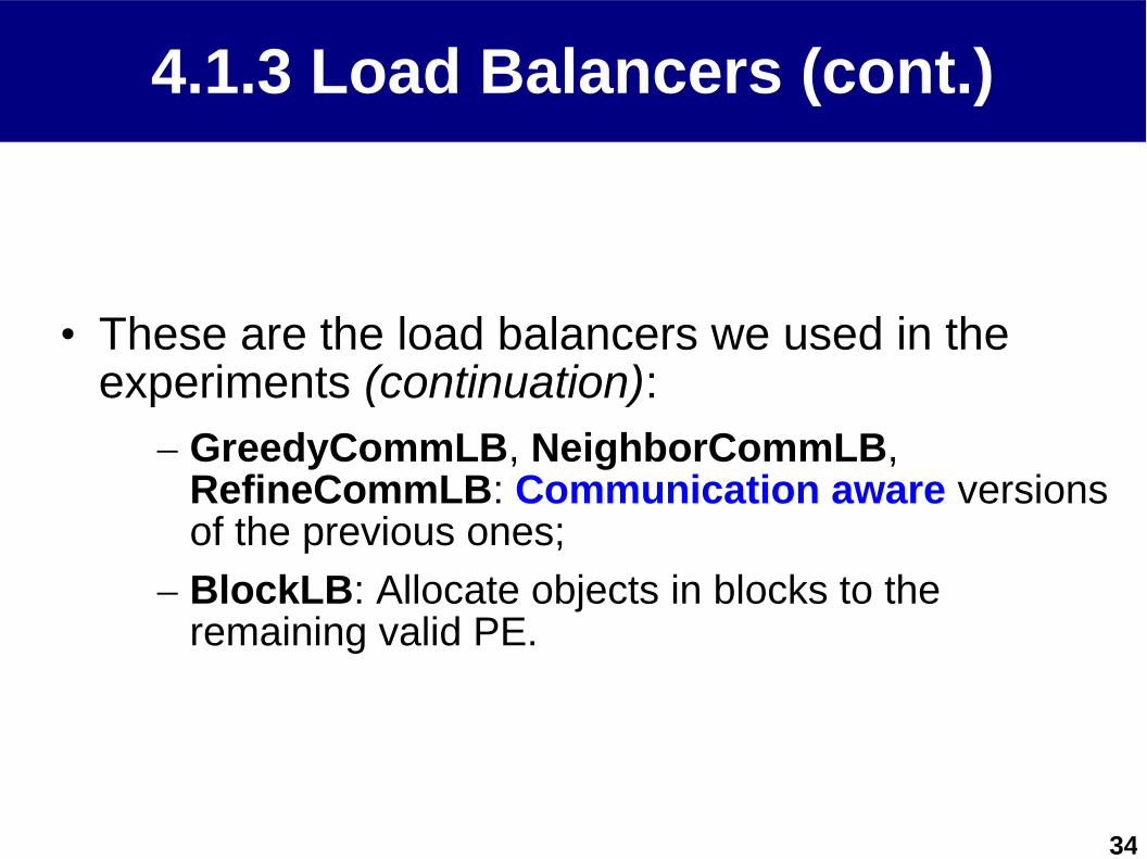
• These are the load balancers we used in the experiments (continuation):
– GreedyCommLB, NeighborCommLB, RefineCommLB: Communication aware versions of the previous ones;
– BlockLB: Allocate objects in blocks to the remaining valid PE.
35
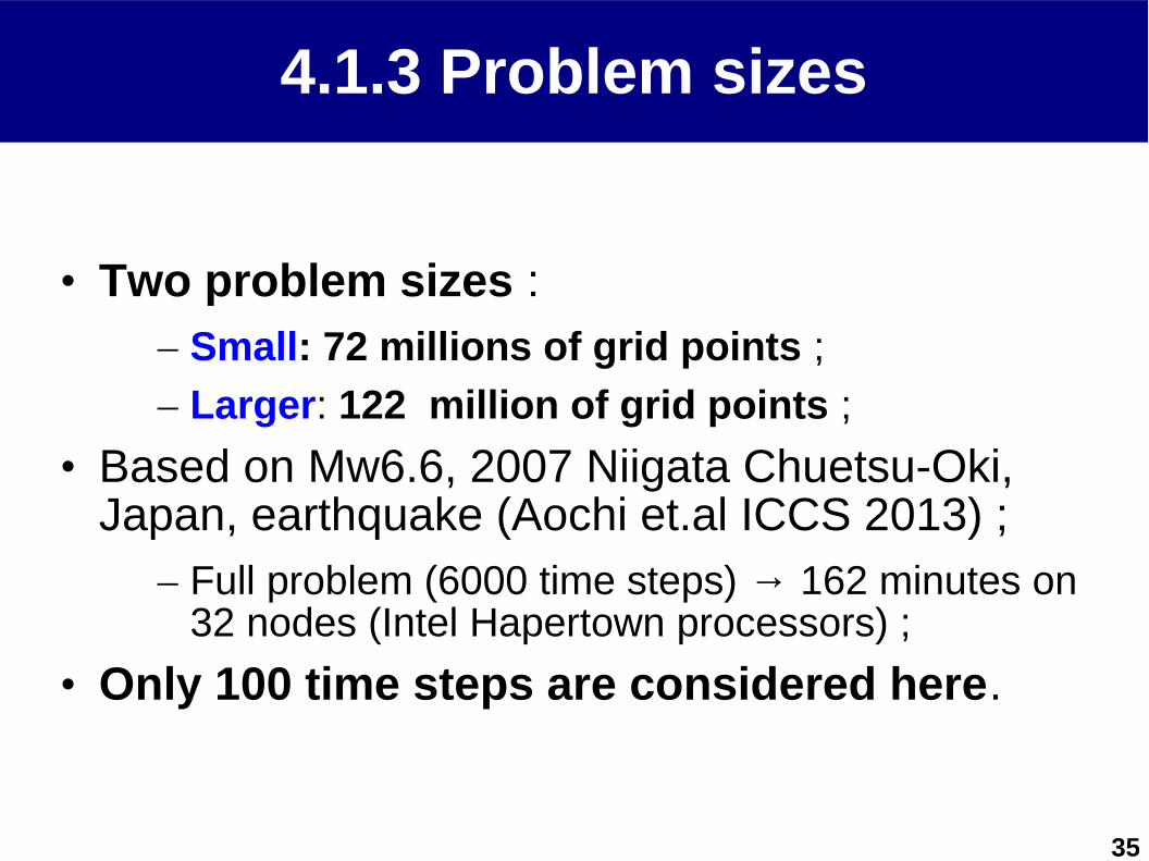
4.1.3 Problem sizes
• Two problem sizes :– Small: 72 millions of grid points ;
– Larger: 122 million of grid points ;
• Based on Mw6.6, 2007 Niigata Chuetsu-Oki, Japan, earthquake (Aochi et.al ICCS 2013) ;
– Full problem (6000 time steps) → 162 minutes on 32 nodes (Intel Hapertown processors) ;
• Only 100 time steps are considered here.
36
4.2 AMPI vs. MPI4.2 AMPI vs. MPI
37
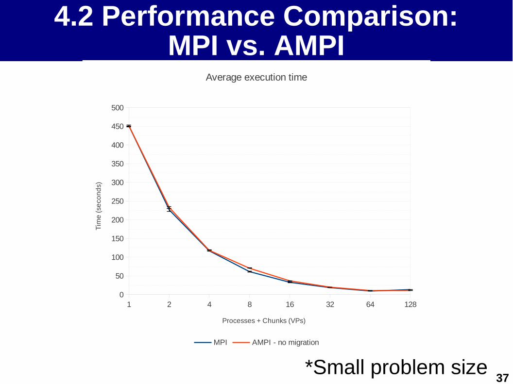
4.2 Performance Comparison:MPI vs. AMPI
1 2 4 8 16 32 64 1280
50
100
150
200
250
300
350
400
450
500
Average execution time
MPI AMPI - no migration
Processes + Chunks (VPs)
Tim
e (
seco
nd
s)
*Small problem size
38
4.3 Statistics from4.3 Statistics fromCharm++/AMPICharm++/AMPI
39
4.3.1 Getting statistics from the AMPI runtime system
• We wanted to detect if Ondes3D's execution was really not load-balanced;
– Module developed by Laércio Pilla (from UFRGS);• Collects statistics used by Charm++/AMPI load
balancers;• Data is collected at each call to MPI_Migrate;
– These experiments were executed with the larger problem size.
• 4 nodes, 32 processes (1 process/core);– 32, 64, 128 virtual processsors;
• 8 nodes, 64 processes (1 process/core);– 64, 128, 256, 640 and 1024 virtual processsors.
40
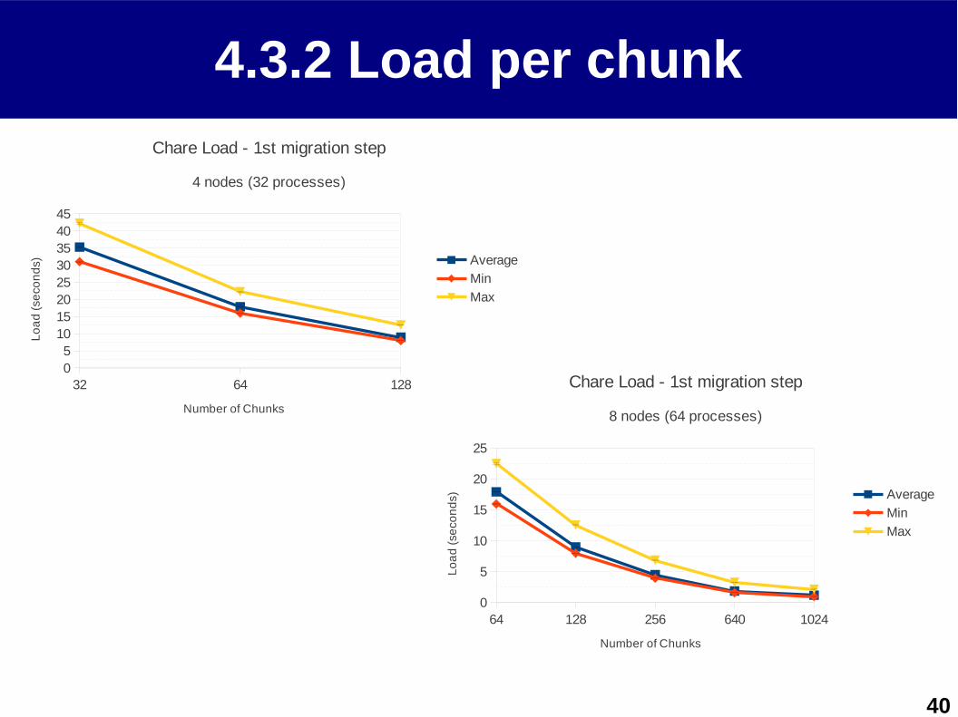
4.3.2 Load per chunk
32 64 12805
1015202530354045
Chare Load - 1st migration step
4 nodes (32 processes)
Average
Min
Max
Number of Chunks
Lo
ad
(se
con
ds)
64 128 256 640 10240
5
10
15
20
25
Chare Load - 1st migration step
8 nodes (64 processes)
Average
Min
Max
Number of Chunks
Lo
ad
(se
con
ds)
41
4.3.3 Difference between max and min loads by chunk
32 64 1280%
10%
20%
30%
40%
50%
60%
70%
Relative Difference Between Max and Min Chare Load
4 nodes (32 processes)
1st step
2nd step
3rd step
4th step
Number of chunks
Diff
ere
nce
64 128 256 640 10240%
20%
40%
60%
80%
100%
120%
140%
Relative Difference Between Max and Min Chare Load
8 nodes (64 processes)
1st step
2nd step
3rd step
4th step
Number of chunks
Diff
ere
nce
42
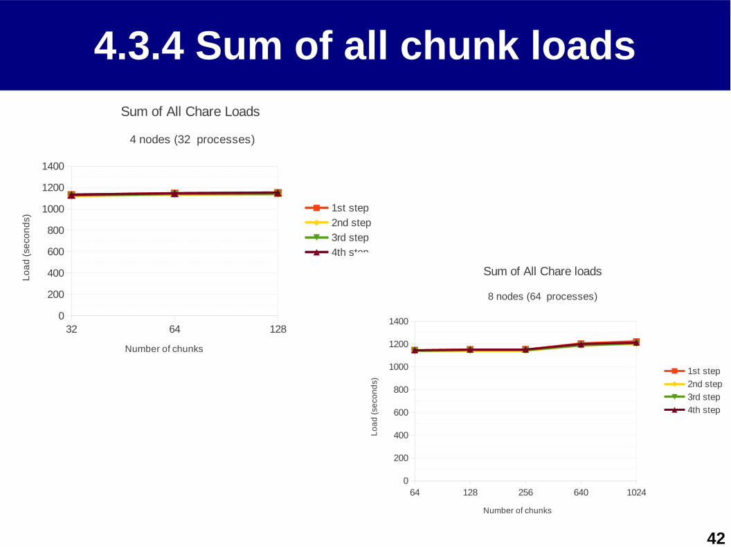
4.3.4 Sum of all chunk loads
32 64 1280
200
400
600
800
1000
1200
1400
Sum of All Chare Loads
4 nodes (32 processes)
1st step
2nd step
3rd step
4th step
Number of chunks
Lo
ad
(se
con
ds)
64 128 256 640 10240
200
400
600
800
1000
1200
1400
Sum of All Chare loads
8 nodes (64 processes)
1st step
2nd step
3rd step
4th step
Number of chunks
Lo
ad
(se
con
ds )
43
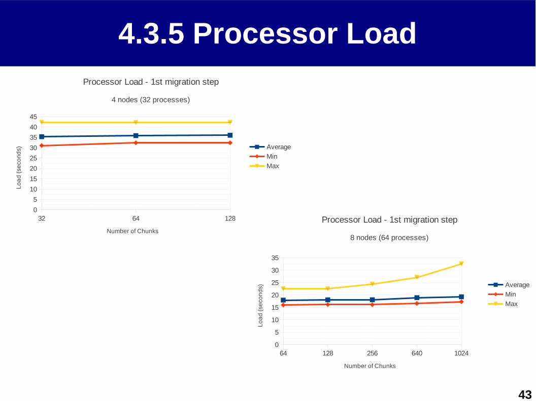
4.3.5 Processor Load
32 64 1280
5
10
15
20
25
30
35
40
45
Processor Load - 1st migration step
4 nodes (32 processes)
Average
Min
Max
Number of Chunks
Lo
ad
(se
con
ds )
64 128 256 640 10240
5
10
15
20
25
30
35
Processor Load - 1st migration step
8 nodes (64 processes)
Average
Min
Max
Number of Chunks
Lo
ad
(se
con
ds )
44
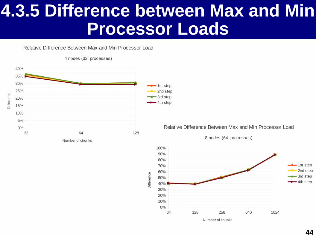
4.3.5 Difference between Max and Min Processor Loads
32 64 1280%
5%
10%
15%
20%
25%
30%
35%
40%
Relative Difference Between Max and Min Processor Load
4 nodes (32 processes)
1st step
2nd step
3rd step
4th step
Number of chunks
Diff
ere
nce
64 128 256 640 10240%
10%
20%
30%
40%
50%
60%
70%
80%
90%
100%
Relative Difference Between Max and Min Processor Load
8 nodes (64 processes)
1st step
2nd step
3rd step
4th step
Number of chunks
Diff
ere
nce
45
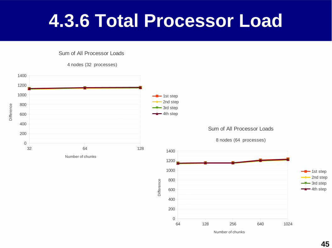
4.3.6 Total Processor Load
32 64 1280
200
400
600
800
1000
1200
1400
Sum of All Processor Loads
4 nodes (32 processes)
1st step
2nd step
3rd step
4th step
Number of chunks
Diff
ere
nce
64 128 256 640 10240
200
400
600
800
1000
1200
1400
Sum of All Processor Loads
8 nodes (64 processes)
1st step
2nd step
3rd step
4th step
Number of chunks
Diff
ere
nce
46
4.4 AMPI performance with4.4 AMPI performance withSMALL problem sizeSMALL problem size
47
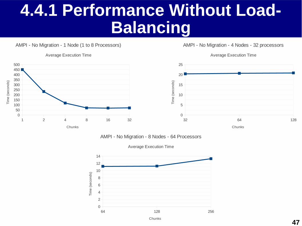
4.4.1 Performance Without Load-Balancing
1 2 4 8 16 320
50100150200250300350400450500
AMPI - No Migration - 1 Node (1 to 8 Processors)
Average Execution Time
Chunks
Tim
e (
seco
nd
s )
32 64 1280
5
10
15
20
25
AMPI - No Migration - 4 Nodes - 32 processors
Average Execution Time
Chunks
Tim
e (
seco
nd
s )
64 128 2560
2
4
6
8
10
12
14
AMPI - No Migration - 8 Nodes - 64 Processors
Average Execution Time
Chunks
Tim
e (
seco
nd
s )
48
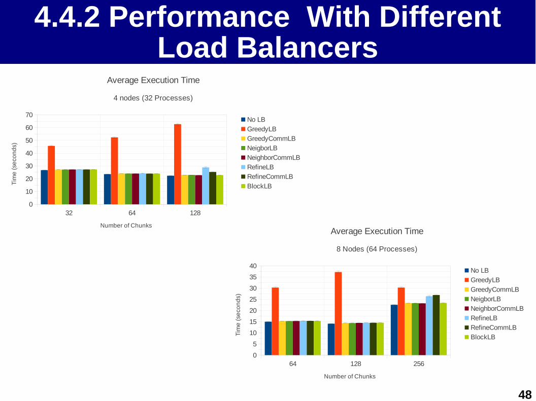
4.4.2 Performance With Different Load Balancers
32 64 1280
10
20
30
40
50
60
70
Average Execution Time
4 nodes (32 Processes)
No LB
GreedyLB
GreedyCommLB
NeigborLB
NeighborCommLB
RefineLB
RefineCommLB
BlockLB
Number of Chunks
Tim
e (
seco
nd
s )
64 128 2560
5
10
15
20
25
30
35
40
Average Execution Time
8 Nodes (64 Processes)
No LB
GreedyLB
GreedyCommLB
NeigborLB
NeighborCommLB
RefineLB
RefineCommLB
BlockLB
Number of Chunks
Tim
e (
seco
nd
s )
49
4.5 AMPI performance with4.5 AMPI performance withLARGER problem sizeLARGER problem size
50
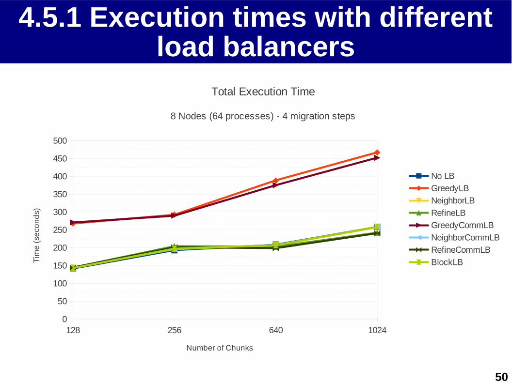
4.5.1 Execution times with different load balancers
128 256 640 10240
50
100
150
200
250
300
350
400
450
500
Total Execution Time
8 Nodes (64 processes) - 4 migration steps
No LB
GreedyLB
NeighborLB
RefineLB
GreedyCommLB
NeighborCommLB
RefineCommLB
BlockLB
Number of Chunks
Tim
e (
seco
nd
s)
51
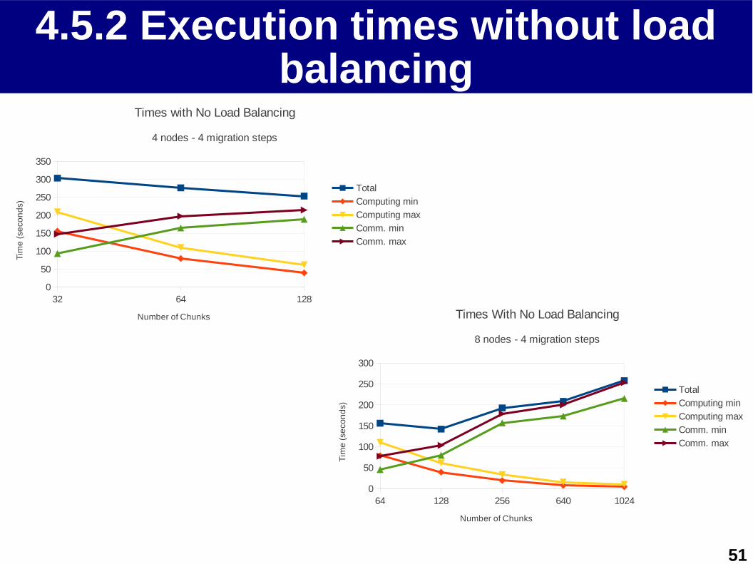
4.5.2 Execution times without load balancing
32 64 1280
50
100
150
200
250
300
350
Times with No Load Balancing
4 nodes - 4 migration steps
Total
Computing min
Computing max
Comm. min
Comm. max
Number of Chunks
Tim
e (
seco
nd
s )
64 128 256 640 10240
50
100
150
200
250
300
Times With No Load Balancing
8 nodes - 4 migration steps
Total
Computing min
Computing max
Comm. min
Comm. max
Number of Chunks
Tim
e (
seco
nd
s )

52
4.5.3 Timings with
128 256 640 10240
50100150200250300350400450500
Times with GreedyLB
8 nodes - 4 migration steps
Total
Computing min
Computing max
Comm. min
Comm. max
Number of Chunks
Tim
e (
seco
nd
s )
128 256 640 10240
50
100
150
200
250
300
Times with NeighborLB
8 nodes - 4 migration steps
Total
Computing min
Computing max
Comm. min
Comm. max
Number of Chunks
Tim
e (
seco
nd
s )

53
5. Final Considerations5. Final Considerations
54
5.1 Final Considerations
• We ported the MPI version of Ondes3D to AMPI;– Performance is similar to MPI version;
• We tested Ondes3D with different load balancers;– 2 different problem sizes;
• Problem: bad computation/communication ratio;– We need to divide the program in small chunks;
– This causes a big increase in the communication overhead per process;
• Why?
55
5.2 Future directions
• More tests with the module developed by Laércio Pilla;
– Using different load balancers;
– Modify the module to get more complete information;
• Get data about the load-balancing;– Migrations performed;
– Duration of migrations;
– Amount of data being migrated;
56
5.2 Future directions (cont.)
• Tests with:– larger systems;
– bigger problem sizes;
• Performance tuning of the code;
• Create a new load-balancer for Charm++;
• Port Ondes3d to Charm++:– Is it worth the effort?
57
5.3 Known issues
• Some known issues:– Migration fails if some modules of Charm++ are
enabled:• ibverbs: infiniband support;• smp: uses threads instead of processes (inside the
same host).
Philippe O. A. Navaux [email protected]
2nd Workshop of the HPC-GA project
Porting Ondes 3D to Adaptive MPI
Informatics Institute, Federal University of
Rio Grande do Sul, Brazil
Parallel and DistributedProcessing Group
Rafael Keller [email protected]
Víctor Martí[email protected]
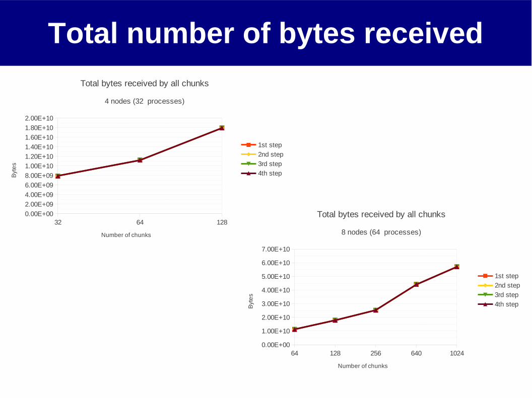
Total number of bytes received
32 64 1280.00E+00
2.00E+09
4.00E+09
6.00E+09
8.00E+09
1.00E+10
1.20E+10
1.40E+10
1.60E+10
1.80E+10
2.00E+10
Total bytes received by all chunks
4 nodes (32 processes)
1st step
2nd step
3rd step
4th step
Number of chunks
Byt
es
64 128 256 640 10240.00E+00
1.00E+10
2.00E+10
3.00E+10
4.00E+10
5.00E+10
6.00E+10
7.00E+10
Total bytes received by all chunks
8 nodes (64 processes)
1st step
2nd step
3rd step
4th step
Number of chunks
Byt
es
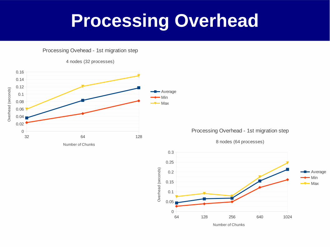
Processing Overhead
32 64 1280
0.02
0.04
0.06
0.08
0.1
0.12
0.14
0.16
Processing Ovehead - 1st migration step
4 nodes (32 processes)
Average
Min
Max
Number of Chunks
Ove
rhe
ad
(se
c on
ds)
64 128 256 640 10240
0.05
0.1
0.15
0.2
0.25
0.3
Processing Overhead - 1st migration step
8 nodes (64 processes)
Average
Min
Max
Number of Chunks
Ove
rhe
ad
(se
c on
ds)

61
32 64 1280
5
10
15
20
25
30
(IB + SMP) vs. (Ethernet - SMP)
Execution time on 4 nodes
No LB No LB smp infiniband
Chunks
Tim
e (
s)
64 128 2560
5
10
15
20
25
(IB + SMP) vs. (Ethernet - SMP)
Execution time on 8 nodes
No LB No LB smp infiniband
Chunks
Tim
e (
s)