Embed Size (px)
Citation preview

Technische Universitat Munchen
Zentrum Mathematik
Portfolio Credit Risk Modelling With
Heavy-Tailed Risk Factors
Krassimir Kolev Kostadinov
Vollstandiger Abdruck der von der Fakultat fur Mathematik der Technischen Universitat
Munchen zur Erlangung des akademischen Grades eines
Doktors der Naturwissenschaften (Dr. rer. nat.)
genehmigten Dissertation.
Vorsitzender: Univ.-Prof. Dr. Folkmar Bornemann
Prufer der Dissertation: 1. Univ.-Prof. Dr.Claudia Kluppelberg
2. Prof. Dr. Liang Peng
Georgia Institute of Technology, Atlanta/USA
Die Dissertation wurde am 17.01.2006 bei der Technischen Universitat eingereicht und
durch die Fakultat fur Mathematik am 07.03.2006 angenommen.

.

Munich University of Technology
Center of Mathematical Sciences
GKAAM
Portfolio Credit Risk Modelling WithHeavy-Tailed Risk Factors
Krassimir Kostadinov
2006

i
Acknowledgments
It is a pleasure for me to thank my advisor Prof. Dr. Claudia Kluppelberg for her patience
and for her support in all aspects of work and life.
The financial support of the Deutsche Forschungsgemeinschaft through the Graduate
Program ”Applied Algorithmic Mathematics” is gratefully acknowledged.
Special thanks to all my colleagues at the graduate program and at the department
for Statistics at the Munich University of Technology for their encouragement throughout
my three years there. Thanks to Gabriel Kuhn and Dr. Martin Hillenbrand for investing
their time and efforts in the area of credit risk modelling and for the numerous fruitful
discussions. Thanks to Christian Schwarz and the other students from the seminar on
credit risk modelling in 2004 for their work and for their challenging questions.
Thanks to Dr. Christian Bluhm for introducing me to the newest practical problems
in the area of credit risk management. Thanks to Prof. Dr. Philip Jorion and to the
anonymous referee from The Journal of Risk for their helpful comments and the suggested
improvements to my paper. Thanks to Dr. Liang Peng for the careful proofreading and
the excellent advises and references he gave me.
I got (unexpectedly for me) really a lot of feedback on my work, from practitioners,
students and researchers at all levels. Thank you all.
Nothing could have been done without the love and support of my family.
ii
Abstract
During the last decade, the dependencies between financial assets have increased due
to globalization effects and relaxed market regulation. The standard industrial methodolo-
gies like RiskMetrics [117] and CreditMetrics [74] model the dependence structure in the
derivatives or in the credit portfolio by assuming multivariate normality of the underlying
risk factors. It has been well recognized that many financial assets exhibit a number of
features which contradict the normality assumption – namely asymmetry, skewness and
heavy tails. Moreover, asset return data suggests also a dependence structure which is
quite different from the Gaussian. Recent empirical studies indicate that especially dur-
ing highly volatile and bear markets the probability for joint extreme events leading to
simultaneous losses in a portfolio could be seriously underestimated under the normality
assumption. Theoretically, Embrechts et al. [48] show that the traditional dependence
measure (the linear correlation coefficient) is not always suited for a proper understand-
ing of the dependency in financial markets. When it comes to measuring the dependence
between extreme losses, other measures (e.g. the tail dependence coefficient) are more
appropriate. This is particularly important in the credit risk framework, where the risk
factors actually enter the model only to introduce a dependence structure in the portfolio.
Clearly, appropriate multivariate models suited for extreme events are needed.
In this thesis, we consider a portfolio credit risk model in the spirit of CreditMet-
rics [74]. With respect to the marginal losses, we retain and enhance all features of that
model and we incorporate not only the default risk, but also the rating migrations, the
credit spread volatility and the recovery risk. The dependence structure in the portfolio
is given by a set of underlying risk factors which we model by a general multivariate el-
liptical distribution. On the one hand, this model retains the standard Gaussian model as
a special case. On the other hand, by introducing a heavy-tailed ”global shock” affecting
the credits simultaneously across regions and business sectors, we obtain a more flexible
model for joint extreme losses.
The goals of the thesis are twofold.
First, we consider the calibration of the model. The main result is a new method
for statistical estimation of the dependence structure (the copula) of a random vector
with arbitrary marginals and elliptical copula. Within our method, we calibrate the linear
correlation coefficients using the whole available sample of observations and the non-linear
(tail) dependence coefficients using only the extreme observations. Special attention is put
to the estimation of the tail dependence coefficients, where additional results aiming at a
iii
lower variance of the estimates are provided. The particular application of the method to
the calibration of the credit risk model is given in detail, and several simulation studies
and real data examples are presented.
Second, we investigate the portfolio loss distribution. In particular, we derive an upper
bound of its tail, which is especially accurate at high loss levels. Given the complexity of
our model, we obtain this result using a mixture of analytic techniques and Monte Carlo
simulation. An approximation of the Value-at-Risk and a new method to determine the
contributions of the individual credits to the overall portfolio risk is provided. The impact
of the heavy-tailed model on the overall portfolio risk and on the risk structure as given
by the risk contributions is investigated. We conclude that the heavy-tailed assumption
has important consequences in all aspects of risk management.

iv

Contents
1 Introduction 1
1.1 Basics of portfolio credit risk modelling . . . . . . . . . . . . . . . . . . . . 1
1.2 The CreditMetrics model . . . . . . . . . . . . . . . . . . . . . . . . . . . . 3
1.3 Generalizations of CreditMetrics . . . . . . . . . . . . . . . . . . . . . . . . 6
1.4 Summary of main results . . . . . . . . . . . . . . . . . . . . . . . . . . . . 7
2 Preliminaries 9
2.1 Copulas and dependence measures . . . . . . . . . . . . . . . . . . . . . . . 9
2.2 Regular variation . . . . . . . . . . . . . . . . . . . . . . . . . . . . . . . . 14
2.2.1 One-dimensional regular variation . . . . . . . . . . . . . . . . . . 14
2.2.2 Multivariate regular variation . . . . . . . . . . . . . . . . . . . . . 18
2.3 Modelling dependence by elliptical distributions . . . . . . . . . . . . . . . 21
3 The model 29
3.1 Heavy-tailed risk factors . . . . . . . . . . . . . . . . . . . . . . . . . . . . 29
3.2 Heavy tails vs CreditMetrics – a first look . . . . . . . . . . . . . . . . . . 32
3.3 Moment generating functions . . . . . . . . . . . . . . . . . . . . . . . . . 35
4 Calibration 43
4.1 Marginal parameters . . . . . . . . . . . . . . . . . . . . . . . . . . . . . . 44
4.1.1 Rating migration probabilities . . . . . . . . . . . . . . . . . . . . 44
4.1.2 Loss given rating . . . . . . . . . . . . . . . . . . . . . . . . . . . . 46
4.2 Bivariate dependence measures . . . . . . . . . . . . . . . . . . . . . . . . 47
4.2.1 Kendall’s tau and correlation . . . . . . . . . . . . . . . . . . . . . 48
4.2.2 Tail dependence . . . . . . . . . . . . . . . . . . . . . . . . . . . . 50
4.3 Elliptical copulae . . . . . . . . . . . . . . . . . . . . . . . . . . . . . . . . 58
4.3.1 Transforming the marginals . . . . . . . . . . . . . . . . . . . . . . 59
4.3.2 Methods based on ML . . . . . . . . . . . . . . . . . . . . . . . . . 60
4.3.3 Methods based on tail dependence . . . . . . . . . . . . . . . . . . 61
v
vi CONTENTS
4.4 Implementation . . . . . . . . . . . . . . . . . . . . . . . . . . . . . . . . . 68
4.5 Numerical examples . . . . . . . . . . . . . . . . . . . . . . . . . . . . . . . 73
5 Simulation 91
5.1 Direct Monte Carlo simulation . . . . . . . . . . . . . . . . . . . . . . . . . 91
5.2 Importance sampling (IS) . . . . . . . . . . . . . . . . . . . . . . . . . . . 92
5.2.1 General IS algorithms . . . . . . . . . . . . . . . . . . . . . . . . . 92
5.2.2 IS for portfolio credit risk . . . . . . . . . . . . . . . . . . . . . . . 94
5.3 Numerical examples . . . . . . . . . . . . . . . . . . . . . . . . . . . . . . . 98
5.3.1 Comparison of the methods . . . . . . . . . . . . . . . . . . . . . . 98
5.3.2 Comparison of the models . . . . . . . . . . . . . . . . . . . . . . . 100
6 Tail approximation 103
6.1 Approximation for large portfolios . . . . . . . . . . . . . . . . . . . . . . . 103
6.2 Approximation by an upper bound . . . . . . . . . . . . . . . . . . . . . . 105
6.3 Numerical examples . . . . . . . . . . . . . . . . . . . . . . . . . . . . . . . 112
7 Application to risk measurement 115
7.1 Risk-adjusted performance measurement . . . . . . . . . . . . . . . . . . . 115
7.2 Risk contributions w.r.t. standard risk measures . . . . . . . . . . . . . . . 116
7.3 Risk contributions w.r.t. tail bound VaR . . . . . . . . . . . . . . . . . . . 118
7.4 Numerical examples . . . . . . . . . . . . . . . . . . . . . . . . . . . . . . 121
7.4.1 Comparison of the methods . . . . . . . . . . . . . . . . . . . . . . 121
7.4.2 Comparison of the models . . . . . . . . . . . . . . . . . . . . . . . 123
8 Conclusions 125

Chapter 1
Introduction
1.1 Basics of portfolio credit risk modelling
Credit risk is a broad category of risks faced by the financial institutions. It includes (see
Duffie and Singleton [40], Chapter 1):
(1) default risk – the risk that an obligor will not be able to meet in time its financial
obligations;
(2) recovery risk – the risk that in case of default the market value of the collateral
of an obligor will not be sufficient to cover at least the expected part of the losses;
(3) credit quality risk – the risk that the credit quality of an obligor, measured by
some internal or external for the financial institution rating system, will decrease;
(4) credit spread risk – the risk of a reduction in the market value of a credit security
(e.g. corporate bond or default swap).
Historically banks have been managing credit risk by imposing rigorous underwriting
standards, credit limit enforcement and one-by-one obligor monitoring. This has changed
dramatically since the late 1990s, when portfolio credit risk has become a key risk manage-
ment challenge (see Allen and Saunders [1], Chapter 1). The amount of credit risk taken
by the banks has increased, and thus the need for more sophisticated techniques. At the
same time, credit derivatives like swaps and forwards have become very popular, lead-
ing to globalization of the credit exposures. In particular, collateralised debt obligations
(CDOs) and other credit risk securities transferring the risk of a whole credit portfolio
have appeared on the market. Last but not least, portfolio credit risk started to play a
crucial role in the determination of capital requirements (see BIS [9]).
The primary reason to have a quantitative portfolio approach to credit risk is that
one can more systematically address the concentration risk. Concentration risk refers to
the additional portfolio risk resulting from an increased exposure to one obligor or groups
of dependent obligors, e.g. by industry, by location, etc. During the last decade, the de-
1
2 CHAPTER 1. INTRODUCTION
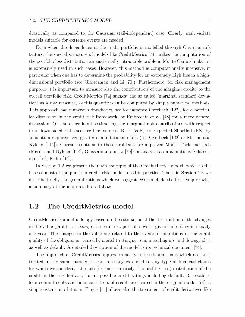
−4 −2 0 2 4−4
−3
−2
−1
0
1
2
3
4T−copula, ν=2, ρ=0.4, N(0,1) marginals
−4 −2 0 2 4−4
−3
−2
−1
0
1
2
3
4Normal copula, ρ=0.4, N(0,1) marginals
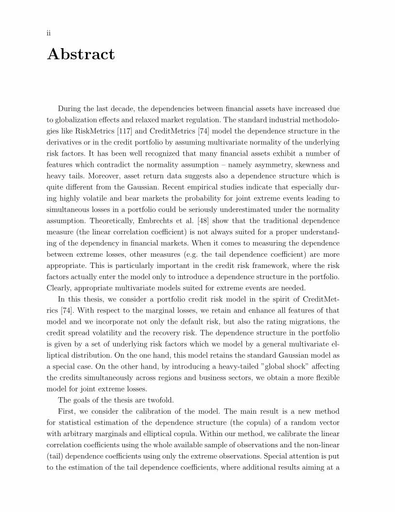
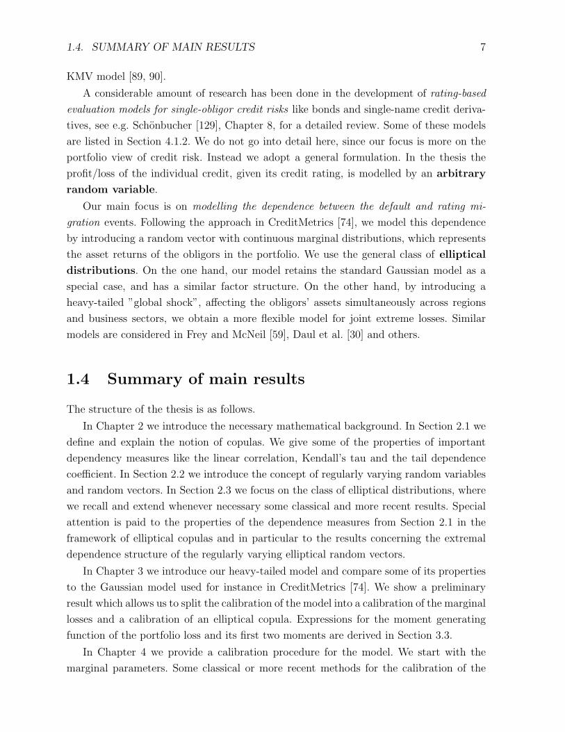
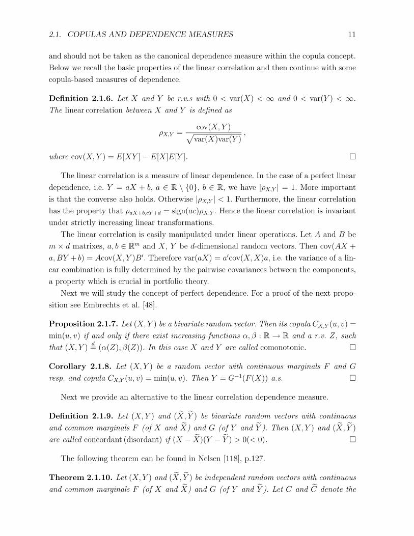
Figure 1.1: The linear correlation is not enough.Left plot: 1000 i.i.d. copies of a bivaraite random vector with standard normal N(0, 1) marginals, corre-lation ρ = 0.4 and t-copula with ν = 4 degrees of freedom (see Example 3.2.1).Right plot: 1000 i.i.d. copies of a bivariate Gaussian random vector with N(0, 1) marginals and corre-lation ρ = 0.4. Obviously there are much more joint extremes in the left plot, indicating a non-lineardependence.The joint extremes are quite important in market VaR analysis and in credit risk.
pendencies between the financial assets in general have increased due to globalization
effects and relaxed market regulation. The standard industrial methodologies like Risk-
Metrics [117] and CreditMetrics [74] model the dependence structure in the derivatives
or in the credit portfolio by assuming multivariate normality of the underlying risk fac-
tors. It has been well recognized (see Mandelbrot [107] for a classsical, or Cont [24] for a
recent study), that many financial assets exhibit a number of features which contradict
the normality assumption – namely asymmetry, skewness and heavy tails. Moreover, as-
set returns data suggests also a dependence structure which is quite different from the
Gaussian (see Fortin and Kuzmics [56]). In particular, empirical studies like Junker and
May [85] and Malevergne and Sornette [106] indicate that, especially during highly volatile
and bear markets, the probability for joint extreme events leading to simultaneous losses
in a portfolio could be seriously underestimated under the normality assumption. Theo-
retically, Embrechts et al. [48] show that the traditional dependence measure (the linear
correlation coefficient) is not always suited for a proper understanding of the dependency
in financial markets. When it comes to measuring the dependence between extreme losses,
other measures (e.g. the tail dependence coefficient) are more appropriate. In the credit
risk framework, Frey et al. [62] provide examples and insight on the impact of a violated
Gaussian assumption on the tail of the credit portfolio loss distribution. Holding the
marginal losses of the individual credits fixed and introducing tail dependence through
heavy-tailed risk factors, Frey et al. [62] conclude that the overall portfolio risk increases
1.2. THE CREDITMETRICS MODEL 3
drastically as compared to the Gaussian (tail-independent) case. Clearly, multivariate
models suitable for extreme events are needed.
Even when the dependence in the credit portfolio is modelled through Gaussian risk
factors, the special structure of models like CreditMetrics [74] makes the computation of
the portfolio loss distribution an analytically intractable problem. Monte Carlo simulation
is extensively used in such cases. However, this method is computationally intensive, in
particular when one has to determine the probability for an extremely high loss in a high-
dimensional portfolio (see Glasserman and Li [70]). Furthermore, for risk management
purposes it is important to measure also the contributions of the marginal credits to the
overall portfolio risk. CreditMetrics [74] suggest the so called ’marginal standard devia-
tion’ as a risk measure, as this quantity can be computed by simple numerical methods.
This approach has numerous drawbacks, see for instance Overbeck [122], for a particu-
lar discussion in the credit risk framework, or Embrechts et al. [48] for a more general
discussion. On the other hand, estimating the marginal risk contributions with respect
to a down-sided risk measure like Value-at-Risk (VaR) or Expected Shortfall (ES) by
simulation requires even greater computational effort (see Overbeck [122] or Merino and
Nyfeler [114]). Current solutions to these problems are improved Monte Carlo methods
(Merino and Nyfeler [114], Glasserman and Li [70]) or analytic approximations (Glasser-
man [67], Kuhn [94]).
In Section 1.2 we present the main concepts of the CreditMetrics model, which is the
base of most of the portfolio credit risk models used in practice. Then, in Section 1.3 we
describe briefly the generalizations which we suggest. We conclude the first chapter with
a summary of the main results to follow.
1.2 The CreditMetrics model
CreditMetrics is a methodology based on the estimation of the distribution of the changes
in the value (profits or losses) of a credit risk portfolio over a given time horizon, usually
one year. The changes in the value are related to the eventual migrations in the credit
quality of the obligors, measured by a credit rating system, including up- and downgrades,
as well as default. A detailed description of the model is its technical document [74].
The approach of CreditMetrics applies primarily to bonds and loans which are both
treated in the same manner. It can be easily extended to any type of financial claims
for which we can derive the loss (or, more precisely, the profit / loss) distribution of the
credit at the risk horizon, for all possible credit ratings including default. Receivables,
loan commitments and financial letters of credit are treated in the original model [74], a
simple extension of it as in Finger [51] allows also the treatment of credit derivatives like
4 CHAPTER 1. INTRODUCTION
swaps and forwards.
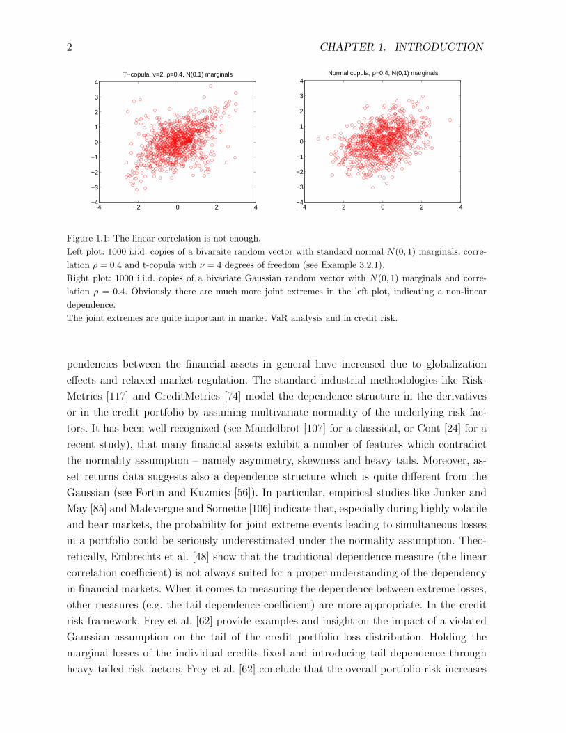
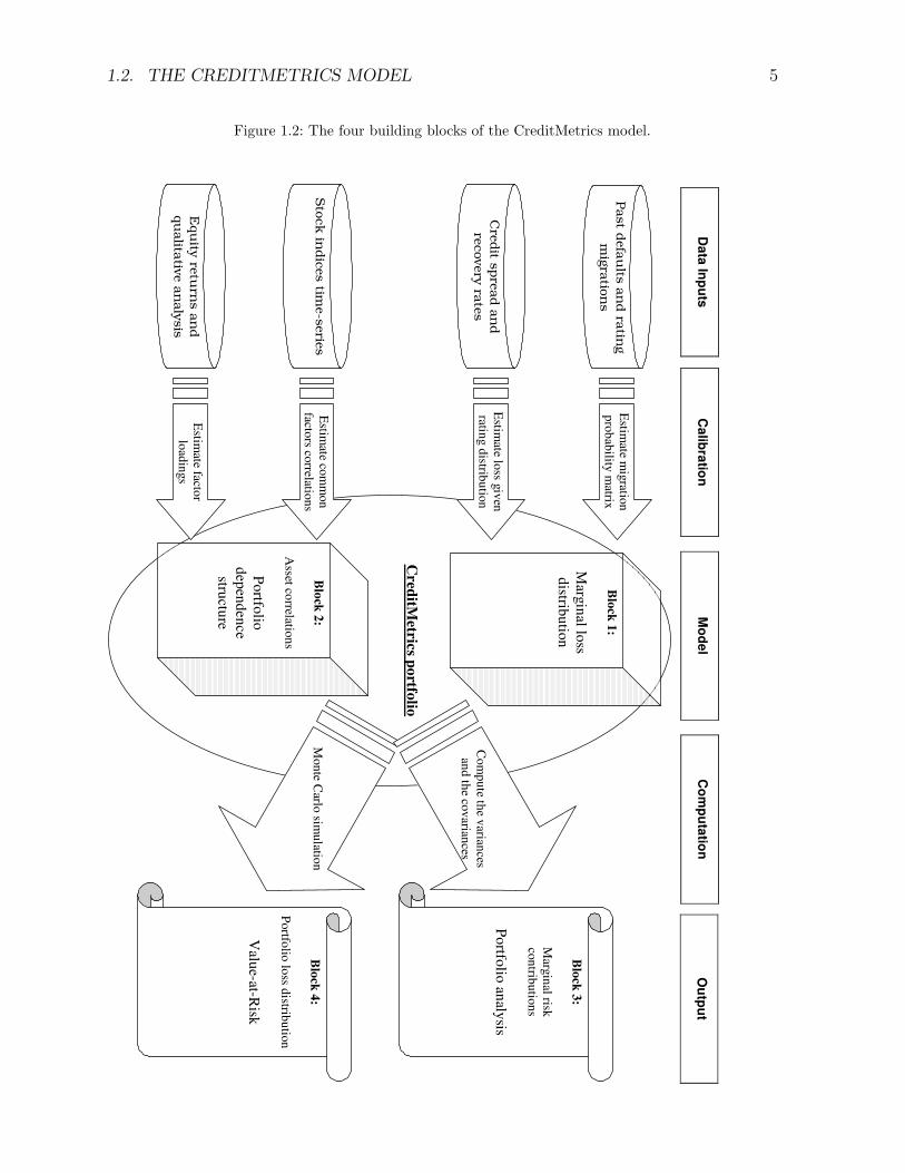
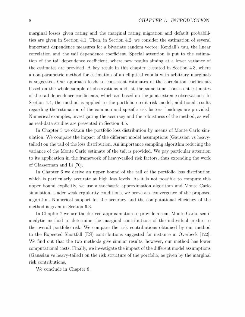
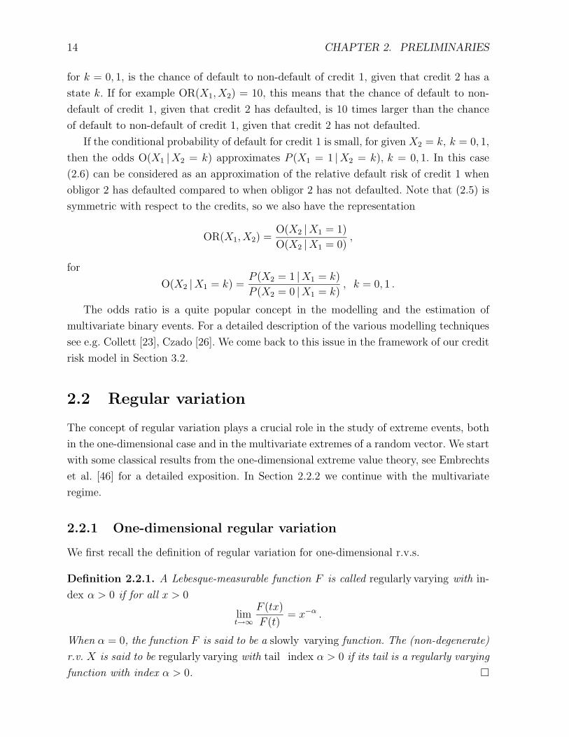
The structure of the model is given in Figure 1.2. There are four ’building blocks’.
In the first building block, the loss distribution at the time horizon of each single credit
in the portfolio is specified separately. In the second one, the multivariate dependence
structure in the portfolio is modelled by means of a set of risk factors. In the third
one, the standard deviation of the portfolio loss and the contribution of every individual
credit to it are computed analytically. In the forth one, Monte Carlo simulation is used
to determine the portfolio loss distribution.
Block 1: First one has to specify a rating system, with rating categories, and as-
sign each of the obligors in the portfolio to an initial rating category. The exact rating
system and the number of rating categories is not significant. It can be Moody’s, or Stan-
dard&Poor’s, or the internal rating system of a bank. However, a strong assumption made
by CreditMetrics is that all obligors are credit-homogeneous within the rating category,
i.e. with the same rating migration probabilities and the same default probability over the
time horizon. These probabilities are collected in a stochastic matrix (migration matrix).
The risk horizon is usually one year, but in principle it can be arbitrary. However, it
should be consistent with the availability of historical default and rating migration data
which is used to calibrate the migration matrix. More details are given in Section 4.1.1,
see also Duffie and Singleton [40], Chapter 4.
Then, one has to specify and calibrate a model for the loss at the risk horizon for each
possible future rating category, including default, for each credit in the portfolio. The
nature and the complexity of this model depends crucially on the type of the credit (e.g.
loan, bond or derivative). Market data like credit spreads, as well as rating agencies’ data
like recovery rates for different obligor classes, is used for the calibration. More details are
given in Section 4.1.2, see also Schonbucher [129], Section 8.5.
Specifying the loss distribution for each possible future rating category and the prob-
ability that the obligor migrates to this category is sufficient to determine the loss distri-
bution at the risk horizon of the single credit (the marginal loss distribution). This
completes the first building block of CreditMetrics.
Block 2: The second building block of CreditMetrics is to specify the dependence
structure in the portfolio. It has been observed (see Nickell et al. [120]), that rating mi-
grations and defaults vary significantly with the business cycle. Furthermore, obligors
operating in the same region (country) and/or business sector tend to default simulta-
neously (over short time intervals). Thus defaults and rating migrations are dependent
events, and a multivariate model for them is needed.
The suggested model is in the spirit of Merton [115]. Default (or rating migration)
is triggered when the asset (log-)returns of the obligor fall below a certain barrier. The
1.2. THE CREDITMETRICS MODEL 5
Figure 1.2: The four building blocks of the CreditMetrics model.
Da
taIn
pu
tsC
om
pu
tatio
nM
od
el
Ca
libra
tion
Ou
tpu
t
Cred
itMetrics
po
rtfolio
Past
defa
ults
an
dra
ting
mig
ratio
ns
Cre
dit
spre
ad
an
d
recovery
rate
s
Sto
ck
indic
es
time-s
erie
s
Equ
ityre
turn
san
d
qu
alita
tive
an
aly
sis
Estim
atem
igratio
n
pro
bab
ilitym
atrix
Estim
atelo
ssgiv
en
rating
distrib
utio
n
Estim
ateco
mm
on
factors
correlatio
ns
Estim
atefacto
r
load
ings
Blo
ck1
:
Marg
inal lo
ss
distrib
utio
n
Blo
ck2
:
Asset
correlatio
ns
Po
rtfolio
dep
end
ence
structu
re
Mon
teC
arlosim
ulatio
n
Com
pu
teth
ev
ariances
and
the
cov
ariances
Blo
ck3
:
Marg
inal
risk
con
tribu
tion
s
Po
rtfolio
analy
sis
Blo
ck4
:
Portfo
liolo
ssd
istribu
tion
Valu
e-at-Risk
6 CHAPTER 1. INTRODUCTION
asset returns are modelled by a multivariate normal random vector. Each asset return is
decomposed into an obligor-specific part and a common part with corresponding loadings
by means of a linear factor model. The correlations between the common factors are
estimated from observable macroeconomic stock indices. The factor loadings are estimated
by a combination of qualitative and quantitative analysis of equity returns data. The
resulting asset correlations are the final output of building block 2. More details are
given in Section 3.1 and in Section 4.4, see also Bluhm et al. [16], Section 2.4.1.
Block 3: The aim of the third building block is to perform a portfolio analysis. The
key issue is to compute the marginal contributions of the individual credits to the overall
portfolio risk. Following the classical theory on portfolio selection (i.e. Markowitz [108]) the
risk is measured by the standard deviation. In the CreditMetrics model, this quantity
can be computed analytically. More details are given in Section 3.3 and in Section 7.2,
see also Tasche [134].
Block 4: It has been well recognized in CreditMetrics [74], that the credit loss dis-
tributions are typically highly skewed and asymmetric. Therefore, knowing the standard
deviation of the portfolio loss distribution (building block 3) is not sufficient to character-
ize the risk of extreme losses, as the standard deviation is a “two-sided” risk measure (see
also Embrechts et al. [48] for a more general discussion). In order to measure the risk of
extreme losses, one needs the tail of the distribution function. Since in the CreditMetrics
model this cannot be computed analytically, a Monte Carlo simulation is applied. The
VaR and other down-sided risk measures are obtained as an output. We present more
details in Section 5.1, see also Glasserman and Li [70].
1.3 Generalizations of CreditMetrics
Various generalizations of the CreditMetrics model are possible.
With respect to the rating modelling, a strong assumption made in CreditMetrics [74]
is that the obligors are credit-homogeneous within a rating category, i.e. the default and
rating migration probabilities are determined by the initial rating category of the obligor.
However, there is a significant amount of evidence that different obligors of the same rating
have different credit qualities, i.e. different default and rating migration probabilities. In
particular, the previous rating of an obligor, the time spent in the current rating, and
the presence of the obligor in watch-lists published by the rating agencies are important
determinants of these probabilities, see Section 4.1.1 and the references therein. For this
reason, in the thesis we consider the marginal default and migration probabilities as
attributes of the individual credit and not of the rating category of the obligor. A
similar extension to the standard CreditMetrics framework is the popular in the industry
1.4. SUMMARY OF MAIN RESULTS 7
KMV model [89, 90].
A considerable amount of research has been done in the development of rating-based
evaluation models for single-obligor credit risks like bonds and single-name credit deriva-
tives, see e.g. Schonbucher [129], Chapter 8, for a detailed review. Some of these models
are listed in Section 4.1.2. We do not go into detail here, since our focus is more on the
portfolio view of credit risk. Instead we adopt a general formulation. In the thesis the
profit/loss of the individual credit, given its credit rating, is modelled by an arbitrary
random variable.
Our main focus is on modelling the dependence between the default and rating mi-
gration events. Following the approach in CreditMetrics [74], we model this dependence
by introducing a random vector with continuous marginal distributions, which represents
the asset returns of the obligors in the portfolio. We use the general class of elliptical
distributions. On the one hand, our model retains the standard Gaussian model as a
special case, and has a similar factor structure. On the other hand, by introducing a
heavy-tailed ”global shock”, affecting the obligors’ assets simultaneously across regions
and business sectors, we obtain a more flexible model for joint extreme losses. Similar
models are considered in Frey and McNeil [59], Daul et al. [30] and others.
1.4 Summary of main results
The structure of the thesis is as follows.
In Chapter 2 we introduce the necessary mathematical background. In Section 2.1 we
define and explain the notion of copulas. We give some of the properties of important
dependency measures like the linear correlation, Kendall’s tau and the tail dependence
coefficient. In Section 2.2 we introduce the concept of regularly varying random variables
and random vectors. In Section 2.3 we focus on the class of elliptical distributions, where
we recall and extend whenever necessary some classical and more recent results. Special
attention is paid to the properties of the dependence measures from Section 2.1 in the
framework of elliptical copulas and in particular to the results concerning the extremal
dependence structure of the regularly varying elliptical random vectors.
In Chapter 3 we introduce our heavy-tailed model and compare some of its properties
to the Gaussian model used for instance in CreditMetrics [74]. We show a preliminary
result which allows us to split the calibration of the model into a calibration of the marginal
losses and a calibration of an elliptical copula. Expressions for the moment generating
function of the portfolio loss and its first two moments are derived in Section 3.3.
In Chapter 4 we provide a calibration procedure for the model. We start with the
marginal parameters. Some classical or more recent methods for the calibration of the
8 CHAPTER 1. INTRODUCTION
marginal losses given rating and the marginal rating migration and default probabili-
ties are given in Section 4.1. Then, in Section 4.2, we consider the estimation of several
important dependence measures for a bivariate random vector: Kendall’s tau, the linear
correlation and the tail dependence coefficient. Special attention is put to the estima-
tion of the tail dependence coefficient, where new results aiming at a lower variance of
the estimates are provided. A key result in this chapter is stated in Section 4.3, where
a non-parametric method for estimation of an elliptical copula with arbitrary marginals
is suggested. Our approach leads to consistent estimates of the correlation coefficients
based on the whole sample of observations and, at the same time, consistent estimates
of the tail dependence coefficients, which are based on the joint extreme observations. In
Section 4.4, the method is applied to the portfolio credit risk model; additional results
regarding the estimation of the common and specific risk factors’ loadings are provided.
Numerical examples, investigating the accuracy and the robustness of the method, as well
as real-data studies are presented in Section 4.5.
In Chapter 5 we obtain the portfolio loss distribution by means of Monte Carlo sim-
ulation. We compare the impact of the different model assumptions (Gaussian vs heavy-
tailed) on the tail of the loss distribution. An importance sampling algorithm reducing the
variance of the Monte Carlo estimate of the tail is provided. We pay particular attention
to its application in the framework of heavy-tailed risk factors, thus extending the work
of Glasserman and Li [70].
In Chapter 6 we derive an upper bound of the tail of the portfolio loss distribution
which is particularly accurate at high loss levels. As it is not possible to compute this
upper bound explicitly, we use a stochastic approximation algorithm and Monte Carlo
simulation. Under weak regularity conditions, we prove a.s. convergence of the proposed
algorithm. Numerical support for the accuracy and the computational efficiency of the
method is given in Section 6.3.
In Chapter 7 we use the derived approximation to provide a semi-Monte Carlo, semi-
analytic method to determine the marginal contributions of the individual credits to
the overall portfolio risk. We compare the risk contributions obtained by our method
to the Expected Shortfall (ES) contributions suggested for instance in Overbeck [122].
We find out that the two methods give similar results, however, our method has lower
computational costs. Finally, we investigate the impact of the different model assumptions
(Gaussian vs heavy-tailed) on the risk structure of the portfolio, as given by the marginal
risk contributions.
We conclude in Chapter 8.
Chapter 2
Preliminaries
2.1 Copulas and dependence measures
In this section we describe the main issues in modelling dependence with copulas. For
more details see Embrechts et al. [47], Joe [83], Nelsen [118]. We summarize the necessary
results without proofs.
Definition 2.1.1. For d ∈ N \ 0 a d-dimensional distribution function (d.f.) with
uniformly distributed on [0, 1] marginals is called copula.
The following theorem is known as Sklar’s Theorem. It is perhaps the most important
result regarding copulas, and is used in essentially all applications of copulas.
Theorem 2.1.2. [Sklar [133]] Let H be a d-dimensional d.f. with marginals F1, . . . , Fd.
Then there exists a copula C such that for all y ∈ Rd
H(y1, . . . , yd) = C(F1(y1), . . . , Fd(yd)) .
If F1, . . . , Fd are all continuous, then C is unique; otherwise C is uniquely determined
on RanF1 × . . . × RanFd. Conversely, if C is a copula and F1, . . . , Fd are d.f.s, then the
function H defined as above is a d-dimensional d.f. with marginals F1, . . . , Fd.
From Sklar’s theorem we see that for continuous multivariate d.f.s., the univariate
marginals and the multivariate dependence structure can be separated, and that the
dependence structure can be represented by a copula.
Corollary 2.1.3. Let H be a d-dimensional d.f. with continuous marginals F1, . . . , Fd
and copula C. Then for every u ∈ [0, 1]d
C(u1, . . . , ud) = H(F−11 (u1), . . . , F−1
d (ud)) ,
where F−1j (uj), j = 1, . . . , d, denotes the generalized inverse function.
9
10 CHAPTER 2. PRELIMINARIES
Let Y be a random vector with continuous marginals F1, . . . , Fd and a joint distribution
H. By means of Theorem 2.1.2 we have
P (Y1 < y1, . . . , Yd < yd) = C(F1(y1), . . . , Fd(yd)) .
Since P (Y1 < y1, . . . , Yd < yd) =∏d
j=1 P (Yj < yj) if and only if the components of Y are
independent, we get the following proposition.
Proposition 2.1.4. If Y is a random vector with continuous marginals, then the compo-
nents of Y are independent if and only if the copula has the form
C(u1, . . . , ud) =d∏j=1
uj .
One nice property of copulas is that for strictly monotone transformations of the
random variables (r.v.s), copulas are either invariant, or change in certain simple ways.
Note that if the d.f. of the r.v. X is continuous, and if α is a strictly monotone function
whose domain contains the range of X (RanX), then the d.f. of α(X) is also continuous.
For a proof of the next proposition see Embrechts et al. [47], Theorems 2.6 and 2.7.
Proposition 2.1.5. Let Y be a random vector with continuous marginals and copula C.
If α1, . . . , αd are strictly increasing functions on RanY1, . . . ,RanYd, respectively, then also
the random vector (α1(Y1), . . . , αd(Yd)) has copula C. If α1, . . . , αd are strictly monotone
on RanY1, . . . ,RanYd, respectively, and, without loss of generality, α1 is strictly decreas-
ing, then
Cα1(Y1),...,αd(Yd)(u1, . . . , ud) = Cα2(Y2),...,αd(Yd)(u2, . . . , ud)−CY1,α2(Y2),...,αd(Yd)(1− u1, u2, . . . , ud) .
Copulas provide a natural way to study the dependence between r.v.s. For practical
purposes, however, it is often needed to summarize the dependence between two r.v.s in
a single number, i.e. to use a dependence measure. As a direct consequence of Proposi-
tion 2.1.5, the dependence measures which are copula properties, i.e. which are determined
only by the copula regardless of the marginals, are invariant under strictly increasing
transformations of the underlying r.v.s.
The linear correlation is most frequently used in practice as a measure of dependence.
However, since the linear correlation is not copula-based, it can often be quite misleading
2.1. COPULAS AND DEPENDENCE MEASURES 11
and should not be taken as the canonical dependence measure within the copula concept.
Below we recall the basic properties of the linear correlation and then continue with some
copula-based measures of dependence.
Definition 2.1.6. Let X and Y be r.v.s with 0 < var(X) < ∞ and 0 < var(Y ) < ∞.
The linear correlation between X and Y is defined as
ρX,Y =cov(X, Y )√
var(X)var(Y ),
where cov(X,Y ) = E[XY ]− E[X]E[Y ].
The linear correlation is a measure of linear dependence. In the case of a perfect linear
dependence, i.e. Y = aX + b, a ∈ R \ 0, b ∈ R, we have |ρX,Y | = 1. More important
is that the converse also holds. Otherwise |ρX,Y | < 1. Furthermore, the linear correlation
has the property that ρaX+b,cY+d = sign(ac)ρX,Y . Hence the linear correlation is invariant
under strictly increasing linear transformations.
The linear correlation is easily manipulated under linear operations. Let A and B be
m× d matrixes, a, b ∈ Rm and X, Y be d-dimensional random vectors. Then cov(AX +
a,BY + b) = Acov(X, Y )B′. Therefore var(aX) = a′cov(X,X)a, i.e. the variance of a lin-
ear combination is fully determined by the pairwise covariances between the components,
a property which is crucial in portfolio theory.
Next we will study the concept of perfect dependence. For a proof of the next propo-
sition see Embrechts et al. [48].
Proposition 2.1.7. Let (X, Y ) be a bivariate random vector. Then its copula CX,Y (u, v) =
min(u, v) if and only if there exist increasing functions α, β : R → R and a r.v. Z, such
that (X, Y )d= (α(Z), β(Z)). In this case X and Y are called comonotonic.
Corollary 2.1.8. Let (X, Y ) be a random vector with continuous marginals F and G
resp. and copula CX,Y (u, v) = min(u, v). Then Y = G−1(F (X)) a.s.
Next we provide an alternative to the linear correlation dependence measure.
Definition 2.1.9. Let (X,Y ) and (X, Y ) be bivariate random vectors with continuous
and common marginals F (of X and X) and G (of Y and Y ). Then (X,Y ) and (X, Y )
are called concordant (disordant) if (X − X)(Y − Y ) > 0(< 0).
The following theorem can be found in Nelsen [118], p.127.
Theorem 2.1.10. Let (X, Y ) and (X, Y ) be independent random vectors with continuous
and common marginals F (of X and X) and G (of Y and Y ). Let C and C denote the
12 CHAPTER 2. PRELIMINARIES
copulas of (X, Y ) and (X, Y ) resp. Denote with τ the probability of concordance minus
the probability of disordance, i.e.
τ = P ((X − X)(Y − Y ) > 0)− P ((X − X)(Y − Y ) < 0) .
Then
τ = 4
∫[0,1]2
C(u, v) dC(u, v)− 1 .
Definition 2.1.11. Kendall′s tau for the bivariate random vector (X, Y ) with continuous
marginals is defined as
τ = P ((X − X)(Y − Y ) > 0)− P ((X − X)(Y − Y ) < 0) , (2.1)
where (X, Y ) and (X, Y ) are independent copies of (X, Y ).
By means of Theorem 2.1.10, the Kendall’s tau is a copula property. As a consequence,
the Kendalls’ tau is invariant under any increasing componentwise transformations (unlike
the linear correlation). For some examples and additional advantages of this dependence
measure see Embrechts et al. [48].
The concept of tail dependence relates to the amount of dependence in the upper-
right-quadrant or the lower-left-quadrant tail of a bivariate distribution. It is a concept
that is relevant for the study of the dependence between extreme events.
Definition 2.1.12. Let (X, Y ) be a random vector with continuous marginal d.f.s F and
G resp. and copula C. The coefficient of lower tail dependence of (X,Y ) is
λL = limu→0
P (X < F−1(u) |Y < G−1(u)) = limu→0
C(u, u)
u, (2.2)
if the limit exists. If λL > 0, (X, Y ) are called lower tail− dependent. Otherwise if λL = 0,
(X, Y ) are called lower tail− independent. In a similar way one may define the coefficient
of upper tail dependence as
λU = limu→1
P (X > F−1(u) |Y > G−1(u)) = limu→1
1− 2u+ C(u, u)
1− u. (2.3)
From (2.2) and (2.3) we find that the tail dependence coefficient is a copula property,
hence the amount of tail dependence is invariant under strictly increasing transformations
on the marginal r.v.s. For copulas without closed analytical form another expression for
the tail dependence coefficient is more useful. Consider a pair of uniformly distributed on
2.1. COPULAS AND DEPENDENCE MEASURES 13
[0, 1] r.v.s (U, V ) with copula C. Note that P (V < v |U = u) = ∂C(u,v)∂u
and P (V > v |U =
u) = 1− ∂C(u,v)∂u
, and similarly when conditioning on V . Then
λL = limu→0
C(u, u)
u
= limu→0
(∂
∂sC(s, t)| s=t=u +
∂
∂tC(s, t)| s=t=u
)(2.4)
= limu→0
(P (V < u |U = u) + P (U < u |V = u)) .
Next we define a more general measure for extremal dependence.
Definition 2.1.13. Let (X, Y ) be a bivariate random vector with continuous marginals
F and G resp. and copula C. For x, y > 0 we call
λ(x, y) = limu→0
1
uP (F (X) < ux,G(Y ) < uy) = lim
u→0
C(ux, uy)
u,
(provided the limit extists) lower tail copula. Similarly one may define an upper tail
copula.
Note that λ(1, 1) in Definition 2.1.13 is exactly equal to the lower tail dependence
coefficient. Furthermore, the tail copula is uniquely determined by the copula of the
random vector, and hence is invariant under marginal transformations.
In Section 2.3 we come back to the dependence measures correlation, Kendall’s tau and
tail dependence, as well as to the tail copula, in the framework of elliptical distributions.
We conclude this section with a definition of a dependence measure which is particularly
suitable for working with discrete binary r.v.s.
Definition 2.1.14. Let X1, X2 be binary 0, 1 r.v.s with P (Xi = 1) = pi > 0, i = 1, 2.
The odds ratio is defined as
OR(X1, X2) =P (X1 = 1, X2 = 1)P (X1 = 0, X2 = 0)
P (X1 = 1, X2 = 0)P (X1 = 0, X2 = 1). (2.5)
For an interpretation of this measure, consider a model where Xi = 1, i = 1, 2, is the
undesirable outcome, e.g. in a simple credit risk model it means the default of obligor i.
Note first that that OR(X1, X2) = 1 if and only X1 and X2 are independent Bernoulli
r.v.s. Further, (2.5) can be rewritten as
OR(X1, X2) =O(X1 |X2 = 1)
O(X1 |X2 = 0), (2.6)
where the odds
O(X1 |X2 = k) =P (X1 = 1 |X2 = k)
P (X1 = 0 |X2 = k),
14 CHAPTER 2. PRELIMINARIES
for k = 0, 1, is the chance of default to non-default of credit 1, given that credit 2 has a
state k. If for example OR(X1, X2) = 10, this means that the chance of default to non-
default of credit 1, given that credit 2 has defaulted, is 10 times larger than the chance
of default to non-default of credit 1, given that credit 2 has not defaulted.
If the conditional probability of default for credit 1 is small, for given X2 = k, k = 0, 1,
then the odds O(X1 |X2 = k) approximates P (X1 = 1 |X2 = k), k = 0, 1. In this case
(2.6) can be considered as an approximation of the relative default risk of credit 1 when
obligor 2 has defaulted compared to when obligor 2 has not defaulted. Note that (2.5) is
symmetric with respect to the credits, so we also have the representation
OR(X1, X2) =O(X2 |X1 = 1)
O(X2 |X1 = 0),
for
O(X2 |X1 = k) =P (X2 = 1 |X1 = k)
P (X2 = 0 |X1 = k), k = 0, 1 .
The odds ratio is a quite popular concept in the modelling and the estimation of
multivariate binary events. For a detailed description of the various modelling techniques
see e.g. Collett [23], Czado [26]. We come back to this issue in the framework of our credit
risk model in Section 3.2.
2.2 Regular variation
The concept of regular variation plays a crucial role in the study of extreme events, both
in the one-dimensional case and in the multivariate extremes of a random vector. We start
with some classical results from the one-dimensional extreme value theory, see Embrechts
et al. [46] for a detailed exposition. In Section 2.2.2 we continue with the multivariate
regime.
2.2.1 One-dimensional regular variation
We first recall the definition of regular variation for one-dimensional r.v.s.
Definition 2.2.1. A Lebesque-measurable function F is called regularly varying with in-
dex α > 0 if for all x > 0
limt→∞
F (tx)
F (t)= x−α .
When α = 0, the function F is said to be a slowly varying function. The (non-degenerate)
r.v. X is said to be regularly varying with tail index α > 0 if its tail is a regularly varying
function with index α > 0.
2.2. REGULAR VARIATION 15
In the one-dimensional case, the extremal behaviour of a sequence of r.v.s can be
illustrated by the behaviour of their maxima. Let (Xn)n∈N be a sequence of r.v.s and
denote Mn = max(X1, . . . , Xn), for n ∈ N \ 0. The following result is the basis of
classical extreme value theory.
Theorem 2.2.2. Let (Xn)n∈N be a sequence of i.i.d. r.v.s with non-degenerate d.f. If there
exist norming constants cn > 0, dn ∈ R, n ∈ N \ 0, and some non-degenerate r.v. M
such that
c−1n (Mn − dn)
d→M ,n→∞ , (2.7)
then the d.f. of M belongs to the type of one of the following three d.f.s.
Frechet: Φα(x) =
0 x ≤ 0 ,
exp (−x−α) x > 0 , α > 0 ;
Weibull: Ψα(x) =
exp (−(−x)α) x ≤ 0 , α > 0 ,
1 x > 0 ;
Gumbel: Λ(x) = exp (−e−x) x ∈ R.
Details of the proof are for instance to be found in Resnik [124], Proposition 0.3. The
three types of d.f.s in Theorem 2.2.2 are called extreme value distributions.
Definition 2.2.3. The d.f. of the r.v. X is said to belong to the maximum domain of
attractition of the extreme value distribution H, if there exist norming constants cn > 0,
dn ∈ R, n ∈ N, such that (2.7) holds and M has d.f. H.
The concept of regular variation is crucial when one has to determine the domain of
attraction of F .
Of particular interest in financial applications are the distributions in the domain of
attraction of the Frechet distribution, see for instance Embrechts et al. [46], Chapter 6.
The next proposition charaterizes the distributions in this domain.
Proposition 2.2.4. The d.f. F belongs to the maximum domain of attraction of the
Frechet distribution Φα, α > 0, if and only if the tail F (x) = x−αL(x), x > 0, where L is
a slowly varying function.
For a proof see Embrechts et al. [46], Theorem 3.3.7. If the r.v. X has d.f. F in the
domain of attraction of Φα, then X is regularly varying and its tail decreases quite slowly
(at a, roughly said, polynomial rate). Note that this implies, for instance, that E[Xβ] =∞for every β ≥ α. Thus, X is a ’heavy-tailed’ r.v.
The following d.f. is a convinient (from a statistical point of view) representation of
the three types of extreme value d.f.s.
16 CHAPTER 2. PRELIMINARIES
Definition 2.2.5. The standardized generalized extreme value distribution (GEV) is
defined as
Hξ(x) =
exp
(−(1 + ξx)−1/ξ
)ξ 6= 0
exp (− exp(−x)) ξ = 0 ,
where the support is
x > −1ξ
ξ > 0
x < −1ξ
ξ < 0
x ∈ R ξ = 0 .
One can introduce the related location-scale family Hξ;µ,σ by replacing the argument x above
with x−µσ
for some µ ∈ R and some σ > 0. The support has to be adjusted accordingly.
We will refer to Hξ;µ,σ as GEV.
In the above definition, ξ = 1/α > 0 corresponds to the Frechet case in Theorem 2.2.2,
ξ = −1/α < 0 to the Weibull case and ξ = 0 to the Gumbel case. Thus, the GEV
distribution describes the limit distribution of normalized maxima of an i.i.d sequence.
An additional topic in extreme value theory is the distribution of scaled excesses over
high thresholds. The following definition makes this notion precise.
Definition 2.2.6. Let X be a r.v. with d.f. F and a right endpoint xF (xF = ∞ is
allowed). For a fixed u < xF
Fu(x) = P (X − u ≤ x |X > u), x > 0
is called the excess distribution of X over the threshold u.
It turns out that the limit behaviour of Fu(x) for u tending to xF can be described by
the following d.f.
Definition 2.2.7. The standardized generalized Pareto distribution (GPD) is defined
as
Gξ(x) =
1− (1 + ξx)−1/ξ ξ 6= 0
1− exp(−x) ξ = 0 ,
where the support is
x ≥ 0 ξ ≥ 0
0 ≤ x ≤ −1ξ
ξ < 0 .
One can introduce the related location-scale family Gξ;µ,σ by replacing the argument x above
with x−µσ
for some µ ∈ R and some σ > 0. The support has to be adjusted accordingly.
We will refer to Gξ;µ,σ as GPD.
2.2. REGULAR VARIATION 17
Theorem 2.2.8. [Embrechts et al. [46], Theorem 3.4.13] Let X be a r.v. with distribution
F . Then F is in the domain of attraction of the extreme value distribution Hξ for some
ξ ∈ R if and only if
limu→xF
sup0<x<xF−u
|Fu(x)−Gξ;0,σ(u)(x)| = 0
for some positive function σ(u).
The extreme value theory is a tool for the analysis and extrapolation of extreme events.
An immense amount of research has been done in the development of the corresponding
statistical methods for extreme events (see Embrechts et al. [46], Chapter 6 for a detailed
overview). One popular suggestion is the Hill estimator for the parameter ξ of the GEV
distribution.
Definition 2.2.9. Let X1, . . . , Xn be i.i.d. r.v.s with d.f. in the domain of attraction of
the Frechet distribution Hξ, ξ > 0. Let X1,n ≥ X2,n ≥ . . . ≥ Xn,n be the ordered sample.
The Hill estimator of ξ takes the form
ξk,n =1
k
k∑j=1
lnXj,n − lnXk,n (2.8)
where k = k(n) is some positive function of the number of observations n, such that
k(n)→∞ and k(n)n→ 0, n→∞.
Theorem 6.4.6. in Embrechts et al. [46] provides conditions for consistency and asymp-
totic normality of ξ. Note that, to apply the estimator we need to select k from the upper
order statistics. Thus, if we select a small k, the estimator has a large variance; otherwise,
if we select a large k, a bias may enter. Methods to find a bias-variance trade-off are given
in e.g. de Haan and Peng [32].
Another popular statistical method in extreme value theory, known as the Peaks-over-
Threshold method (POT), is based on Theorem 2.2.8. Note that the density of the GPD
with parameters ξ and σ is explicitly available:
gξ;σ(x) =1
σ
(1 + ξ
x
σ
)−1/ξ−1
, x ∈ supp(Gξ;σ) .
Therefore, given a sample Y1, . . . , Yn of i.i.d. r.v.s with GPD, the log-likelihood function
equals
l(ξ, σ; Y ) = −n lnσ −(
1
ξ+ 1
) n∑i=1
ln
(1 + ξ
Yiσ
). (2.9)
Let now X1, . . . , Xn be a sample of i.i.d. r.v.s with d.f. F (x) = P (X ≤ x) in the domain
of attraction of the Frechet distribution Φα. We select a high threshold u and denote
18 CHAPTER 2. PRELIMINARIES
Nu = #i : Xi > u and the corresponding excesses Y1, . . . , YNu . For every x > u we
have
P (X > x) = P (X > u)P (X > x |X > u) .
The Glivenko-Cantelli theorem suggests to approximate P (X > u) with the empirical
d.f., i.e. with Nun
, for a range where there are still enough data to guarantee good ap-
proximation. Theorem 2.2.8 suggests to approximate P (X > x |X > u) with the GPD
Gξ;σ(x−u) with the appropriate parameters ξ and σ, introducing a semiparametric model,
where data are sparse. Maximum likelihood (ML) estimates for ξ and σ can be found by
using the excesses Y1, . . . , YNu from the sample and maximizing numerically (2.9).
For the asymptotic theory behind this method see Smith [132]. As with the Hill esti-
mator, a key point is the selection of the threshold u, where a bias-variance trade-off is
sought, see the discussion on p.355 in Embrechts et al. [46].
2.2.2 Multivariate regular variation
In this section we give some basic results on multivariate regular variation, for details see
Kallenberg [86]. To prepare for the definition of regular variation for random vectors, we
recall the concept of vague convergence. Let χ be a separable metric space. A set B ⊂ χ is
said to be relatively compact if its closure B is compact. Let σ(χ) be the Borel σ-algebra
on χ. A measure µ on (χ, σ(χ)) is called a Radon measure if µ(B) <∞ for all relatively
compact sets B ∈ σ(χ).
Definition 2.2.10. Let µ, µ1, µ2, . . . be Radon measures on (χ, σ(χ)). We say that µn
converges to µ vaguely, if
limn→∞
∫χ
f(s)µn(ds) =
∫χ
f(s)µ(ds)
for all continuous functions f : χ→ R+ with compact support. We denote µn
v→ µ.
A useful equivalent formulation of vague convergence is given in the following theorem.
Theorem 2.2.11. Let µ, µ1, µ2, . . . be Radon measures on (χ, σ(χ)). Then µn converges
to µ vaguely, if and only if
limn→∞
µn(B) = µ(B)
for all relatively compact B ∈ σ(χ) with µ(∂B) = 0.
For a proof see Kallenberg [86], p.169.
2.2. REGULAR VARIATION 19
Definition 2.2.12. The d-dimensional random vector Y is said to be regularly varying
with tail index α > 0 if there exists a random vector Θ with values in Sd−1 = y ∈ Rd :
|y| = 1 such that for all y > 0
P (|Y | > ty, Y|Y | ∈ ·)P (|Y | > t)
v→ y−αP (Θ ∈ ·), t→∞ . (2.10)
The distribution of Θ is referred to as the spectral measure of Y .
Remark 2.2.13. In Definition 2.2.12 we do not specify the choice of a norm | · |. The
reason for this is that whether a random vector is regularly varying or not does not depend
on the choice of norm, see Hult and Lindskog [78]. In particular, the tail index α in (2.10)
remains the same irrespective of the selected norm.
Although the property of multivariate regular variation is norm-independent, the form
of the spectral measure is certainly not. Frequently encountered norms include the Eu-
clidean L2-norm
|Y | =
√√√√ d∑i=1
Y 2i
and the max-norm
|Y |max = max(|Y1|, . . . , |Yd|) .
In what follows | · | denotes an arbitrary norm, unless stated otherwise. The choice of a
norm for a given situation is a problem in its own right. Clearly, the max-norm is large as
soon as at least one of the components of Y is large. Whether the other components are
large or not is not of interest. In the Euclidean norm, on the other hand, we need not have
any component of Y extremely large in order for |Y | to be large, since the components
of Y jointly determine |Y |. The max-norm might therefore be useful in models where
always the largest component outcome as such is of interest, while the Euclidean norm
pays attention to all components of Y . Before starting to model multivariate extremes it
might be worthwhile giving some thought to the choice of norm.
A useful fact contained in the next proposition concerns the effect of additive constants
in the multivariate regular variation settings.
Proposition 2.2.14. Let Y be a d-dimensional regularly varying random vector with tail
index α > 0 and spectral measure PΘ w.r.t. some norm | · | and let b ∈ Rd be a constant
vector. Then Y + b is regularly varying with the same tail index α and the same spectral
measure w.r.t. the norm | · |.
For a proof see Hult and Lindskog [78].
The next proposition presents a link between regularly varying vectors and their norms.
20 CHAPTER 2. PRELIMINARIES
Proposition 2.2.15. Let Y be a d-dimensional regularly varying random vector with tail
index α. Then |Y | is a regularly varying r.v. in the sense of Definition 2.2.1 with tail
index α.
For a proof see Wendin [135], Proposition 1.3. Theorem 1.1 in the same work states
the result to follow, see also Theorem 2.2.11 and Basrak [10].
Proposition 2.2.16. Let Y be a d-dimensional random vector with support on the whole
space of Rd. Then Y is regularly varying with tail index α if and only if there exists a
sequence of norming constants an > 0 and a non-zero Radon measure µ such that
nP (a−1n Y > ·) v→ µ(·) . (2.11)
Moreover, for every t > 0 and for every relatively compact set B ∈ σ(χ) with µ(∂B) = 0,
µ(tB) = t−αµ(B)
Remark 2.2.17. The Radon measure in (2.11) is unique up to a multiplicative constant.
Proposition 2.2.16 implies also the existence of constants an > 0, n ∈ N, such that for
the marginals of the random vector Y holds
nP (a−1n Yi > x)→ cix
−α , n→∞ ,
where ci ≥ 0, i = 1, . . . , d. Unfortunatelly nothing guarantees that the constants ci are
strictly positive. Non-positive constants may occur, for instance, when the marginals of
Y are regularly varying with different tail indices, see p.11 in Mikosch [116].
Our next aim is to present a consistent estimator of the Radon measure µ in Propo-
sition 2.2.16.
Let | · | be an arbitrary norm and let Y be a regularly varying random vector with
tail index α. Denote by F the d.f. of |Y | and by F−1 its generalized inverse function. A
possible choice of norming constants in (2.11) is an = F−1(1/n), see Proposition 2.2.15
and Resnick [124], Proposition 1.11. Then we introduce the auxiliary sequence k = k(n)
with the properties k(n)→∞ and k(n)n→ 0 as n→∞. Because of (2.11),
n
kP (
1
F−1(k/n)Y ∈ ·) v→ µ(·) , n→∞ .
Consequently, with Y (1) . . . , Y (n) being i.i.d copies of Y, we obtain
µn(·) =1
k
n∑i=1
1Y (i)/F−1E (k/n)∈·
v→ µ(·) , n→∞ , (2.12)
where F−1E (x) denotes the inverse of the empirical d.f. of |Y |. For details of the proof see
e.g. Wendin [135].
2.3. MODELLING DEPENDENCE BY ELLIPTICAL DISTRIBUTIONS 21
2.3 Modelling dependence by elliptical distributions
The main topic of this section is to understand the various measures of dependence
through elliptical distributions. First we introduce the class of elliptically distributed
random vectors and give some of their properties. For further details about elliptical
distributions we refer to Fang et al. [50].
Definition 2.3.1. If Y is a d-dimensional random vector and, for some vector µ ∈ Rd,some d× d non-negative definite symmetric matrix Σ and some function φ : [0,∞)→ R,
the characteristic function of Y − µ is of the form ϕY−µ(t) = φ(t′Σt), we say that Y has
an elliptical distribution with parameters µ, Σ and φ. The function φ is referred to as the
characteristic generator of Y .
When d = 1, the class of elliptical distributions coincides with the class of one-
dimensional symmetric distributions.
For elliptically distributed random vectors, we have the following general representa-
tion theorem see Fang et al. [50], Theorem 1.3.
Theorem 2.3.2. The d-dimensional random vector Y is elliptically distributed with pa-
rameters µ, Σ (rank(Σ) = k) and φ, if and only if there exist a non-negative r.v. R,
independent of U , a k-dimensional random vector uniformly distributed on the unit hy-
persphere Sk =z ∈ Rk : z′z = 1
, and a d× k matrix A with AA′ = Σ, such that
Y = µ+RAU . (2.13)
Remark 2.3.3. Uniqueness of the representation:
(1) Representation (2.13) is not unique: if B is an orthogonal k×k matrix, then (2.13)
holds also with Anew = AB and Unew = B′U .
(2) Elliptical distributions with different parameters can in fact be equal: for every
c > 0, Yd= Ynew, where Ynew has parameters µ, cΣ and φ( ·
c), or, alternatively, Rnew =
R/√c in (2.13)
In this work we are going to use frequently the class of normal variance mixture
distributions (NVM).
Definition 2.3.4. Let Z be a d-dimensional normal random vector with zero mean and
covariance matrix Σ with rank(Σ) = d (Z ∈ Nd(0,Σ)). Let W > 0 be a r.v., indepen-
dent of Z and µ ∈ Rd be a constant vector. Then we say that Y = µ + WZ has a
normal variance mixture distribution (Y ∈ Nd(µ,W2Σ)).
22 CHAPTER 2. PRELIMINARIES
Remark 2.3.5. Note that the NVM distributions are a subclass of the elliptical distribu-
tions. To see this we take an arbitrary NVM Y = µ+WZ and we let R = W√χ2d, where
χ2d is a chi-square distributed r.v., independent of W . We obtain for the NVM distribution
Y = µ+WZd= µ+RAU , where A is a matrix such that AA′ = Σ and U is a d-dimensional
random vector uniformly distributed on the unit hypersphere Sd =z ∈ Rd : z′z = 1
–
i.e. Y is elliptical by means of (2.13). In particular, Y is t-distributed with ν degrees of
freedom if R2/d ∈ F (d, ν) (F -distribution with d and ν degrees of freedom), or, equiva-
lently, W =√
νχ2ν. Most of the known elliptical distributions can be represented as NVM,
see Fang et al. [50], Theorem 2.21 for details.
Remark 2.3.6. If the NVM Y has finite second moments, then we can always find a
representation such that cov(Y ) = Σ. To see this we observe that cov(Y ) = cov(µ+WZ) =
E[W 2]cov(AZI), where A is a matrix such that AA′ = Σ (Choleski decomposition) and
ZI is a vector of independent standard normals. Then cov(Y ) = E[W 2]Σ. So, as in
Remark 2.3.3 (2) we set c = E[W 2].
The following result provides the basis of most applications of elliptical distributions.
Lemma 2.3.7. Let Y be d-dimensional elliptically distributed random vector with param-
eters µ, Σ and φ and let B be a q×d matrix and b ∈ Rq. Then b+BY is a q-dimensional
elliptically distributed random vector with parameters µnew = b + Bµ, Σnew = BΣB′ and
φ.
Proof. By Theorem 2.3.2, b+BYd= b+Bµ+RBAU .
If we partition Y , µ and Σ into Y = (Y1, Y2)′, µ = (µ1, µ2)′ and Σ =
(Σ11 Σ12
Σ21 Σ22
),
where Y1 and µ1 are r-dimensional vectors (r < d) and Σ11 is a r× r matrix, we have the
following consequence of Lemma 2.3.7.
Corollary 2.3.8. If Y is a d-dimensional elliptically distributed random vector with pa-
rameters µ, Σ and φ, then Y1 and Y2 are resp. r and d − r dimensional elliptically dis-
tributed vectors with parameters resp. µ1, Σ11, φ and µ2, Σ22, φ.
Hence, marginal distributions of the elliptical distributions are elliptical and of the
same type (with the same characteristic generator).
We start to investigate the dependence structure of the elliptical distributions.
Definition 2.3.9. Let Y be a d-dimensional elliptically distributed random vector with
parameters µ, Σ and φ. We call
ρij =Σij√ΣiiΣjj
, i, j = 1, . . . , d, (2.14)
correlation coefficient.
2.3. MODELLING DEPENDENCE BY ELLIPTICAL DISTRIBUTIONS 23
We observe that if var(Yi) < ∞ and var(Yj) < ∞, then ρij in the above definition is
the usual linear correlation, i.e. ρij =cov(Yi,Yj)√
var(Yi)var(Yj). However, for elliptical distributions
ρij is well defined even when linear correlation is not.
Corollary 2.3.10. Let Y be d-dimensional elliptically distributed random vector with
parameters µ, Σ and φ. If the marginals of Y are continuous, then the copula of Y is
uniquely determined by φ and [ρij]i,j=1,...,d.
Proof. We observe that due to Proposition 2.1.5 Y has the same copula as the vector Ynew
obtained from Y by substracting the means µi and multiplying by (Σii)−1/2 component-
wise for i = 1, . . . , d. By Lemma 2.3.7 we have that Ynew has elliptical distribution with
parameters µnew = 0, Σnew = [ρij]i,j=1,...,d and φnew = φ.
The relation between the Kendall’s tau (2.1) and the linear correlation coefficient
is well known for bivariate normally distributed random vectors. In the next theorem
we state a more general relation between the Kendall’s tau and the correlation ρij for
elliptically distributed random vectors.
Theorem 2.3.11. [Lindskog et al. [104]] Let Y be a d-dimensional elliptically distributed
random vector with absolutely continuous marginals with support on the whole of R. Then
the following relation holds:
τ(Yi, Yj) =2
πarcsin ρij , i, j = 1, . . . , d . (2.15)
The next theorem clarifies the relation between regular variation and tail dependence
for an elliptically distributed random vector. Recall Definitions 2.1.12, 2.2.1 and 2.2.12.
Proposition 2.3.12. Let Y be a d-dimensional elliptically distributed random vector with
absolutely continuous marginals with support on the whole of R and representation Y =
µ+RAU as in (2.13). Then the following statements are equivalent:
(1) R is regularly varying with tail index α > 0;
(2) Y is regularly varying with tail index α > 0;
(3) for all i, j = 1, . . . , d, i 6= j, the vector (Yi, Yj) is tail dependent. Moreover, the
coefficients of tail dependence are given by
λU(Yi, Yj) = λL(Yi, Yj) =
∫ π2
g(ρij)cosα t dt∫ π
2
0cosα t dt
, (2.16)
where g(ρij) = π4− arcsin ρij
2= π
4(1 − τij) and ρij and τij are the correlation coefficient in
(2.14) and Kendall’s tau in (2.1), respectively.
24 CHAPTER 2. PRELIMINARIES
Proof. It has been shown by Hult and Lindskog [78], that (1) and (2) are equivalent, as
well as that from (1) follows (3). The same paper states also the result, that if for all
i, j = 1, . . . , d, i 6= j, the vector (Yi, Yj) is tail dependent, then R is regularly varying with
some index β > 0 (possibly β 6= α), such that∫ π2
g(ρij)cosα t dt∫ π
2
0cosα t dt
=
∫ π2
g(ρij)cosβ t dt∫ π
2
0cosβ t dt
.
However, if β 6= α, then this contradicts to Lemma 2.3.13 (3).
In the next lemma we analyze further the function on the right-hand side of (2.16).
Lemma 2.3.13. Setting x = π4(1− τ) in (2.16), we define
λ(α, x) =
∫ π2
xcosα t dt∫ π
2
0cosα t dt
, α ≥ 0, x ∈ [0,π
2] .
It satisfies the following properties.
(1) λ(α, x) is continuous and differentiable in α > 0, x ∈ (0, π2).
(2) 0 < λ(α, x) < 1.
(3) Let x ∈ (0, π2) be fixed. Then λ(α, x) is strictly decreasing in α > 0. Furthermore,
limα→0
λ(α, x) = 1− 2x
π, lim
α→∞λ(α, x) = 0 .
(4) Let α > 0 be fixed. Then λ(α, x) is strictly decreasing in x ∈ (0, π2).
Proof. The function cosα t for t ∈ (0, π2) is continuous and differentiable, and so are∫ π
2
xcosα t dt and
∫ π2
0cosα t dt as functions of α > 0 and of x ∈ (0, π
2). Furthermore, cosα t >
0 for t ∈ (0, π2), hence 0 <
∫ π2
xcosα t dt <
∫ π2
0cosα t dt, therefore we obtain (2).
To prove (3) we differentiate with respect to α
∂
∂αλ(α, x) =
∫ π2
0cosα t dt
∫ π2
xlog (cos t) cosα t dt−
∫ π2
xcosα t dt
∫ π2
0log (cos t) cosα t dt(∫ π
2
0cosα t dt
)2
=D(α, x)(∫ π
2
0cosα t dt
)2 .
We will prove that D(α, x) < 0 for every x ∈ (0, π2) and α > 0.
First we note that D(α, 0) = D(α, π2) = 0. Then we differentiate with respect to x:
∂
∂xD(α, x) = − log (cos x) cosα x
∫ π2
0
cosα t dt+ cosα x
∫ π2
0
log (cos t) cosα t dt
= cosα x
(− log (cos x)
∫ π2
0
cosα t dt+
∫ π2
0
log (cos t) cosα t dt
)= C(α, x) cosα x .
2.3. MODELLING DEPENDENCE BY ELLIPTICAL DISTRIBUTIONS 25
Note that
C(α, 0) =
∫ π2
0
log (cos t) cosα t dt < 0
and that
limx→π
2
C(α, x) =∞
and that C(α, x) is strictly increasing in x for x ∈ (0, π2), as − log (cos x) is strictly increas-
ing. Therefore there exists a unique point y, 0 < y < π2, such that C(α, y) = 0. Further-
more, ∂∂xD(α, x) = C(α, x) cosα x < 0 for x ∈ (0, y) and ∂
∂xD(α, x) = C(α, x) cosα x > 0
for x ∈ (y, π2), so D(α, x) is strictly decreasing for x ∈ (0, y) (i.e decreasing from D(α, 0) =
0 to D(α, y) < 0) and D(α, x) is strictly increasing for x ∈ (y, π2) (i.e. increasing from
D(α, y) < 0 to D(α, π2) = 0). Therefore D(α, x) < 0 for x ∈ (0, π
2) and α > 0. Therefore
∂∂αλ(α, x) < 0 for x ∈ (0, π
2) and α > 0, which proves that λ(α, x) is strictly decreasing.
Furthermore,
limα→0
λ(α, x) = limα→0
∫ π2
xcosα t dt∫ π
2
0cosα t dt
= 1− 2x
π.
Taking some 0 < ε < x and using the fact that cosα t is strictly decreasing in t for every
α > 0 we obtain
1
λ(α, x)=
∫ π2
0cosα t dt∫ π
2
xcosα t dt
=
∫ ε0
cosα t dt∫ π2
xcosα t dt
+
∫ π2
εcosα t dt∫ π
2
xcosα t dt
≥ ε cosα ε
(π2− x) cosα x
+ 1 .
Since(
cos εcosx
)α →∞ as α→∞, we obtain
limα→∞
λ(α, x) = 0 .
As cosα t > 0 for t ∈ (0, π2), we have also the monotonicity of
∫ π2
xcosα t dt, i.e. (4).
From Proposition 2.3.12 we may conclude that the bivariate marginals of an elliptically
distributed random vector Y are tail-dependent if and only if the spectral r.v. R in (2.13) is
regularly varying. Kendall’s tau τij only affects the magnitude of the tail dependence. As a
consequence of the proposition, r.v.s with a Gaussian copula are tail-independent, whereas
the t-copula with ν degrees of freedom leads to a tail dependence with α = ν. Furthermore,
due to Lemma 2.3.13 (3) we find that the smaller the tail index α of the spectral r.v. R is
(i.e. the heavier the tails of Y1, . . . , Yd are), the higher are the tail dependence coefficients.
Note that the tail dependence coefficients depend on the distribution of R only through
the tail index α. In the next corrolary we state the result for NVM random vectors.
26 CHAPTER 2. PRELIMINARIES
Proposition 2.3.14. Let Y = µ + WZ be a d-dimensional NVM random vector. Then
the following statements are equivalent:
(1) W is regularly varying with tail index α > 0;
(2) Y is regularly varying with tail index α > 0;
(3) for all i, j = 1, . . . , d, i 6= j, the vector (Yi, Yj) is tail dependent. Moreover, the
coefficients of tail dependence are given by
λU(Yi, Yj) = λL(Yi, Yj) =
∫ π2
g(ρij)cosα t dt∫ π
2
0cosα t dt
, (2.17)
where g(ρij) = π4− arcsin ρij
2= π
4(1 − τij) and ρij and τij are the correlation coefficient in
(2.14) and Kendall’s tau in (2.1), respectively.
Proof. By Breimann’s classical result (see Breimann [17]), the r.v. R = W√χ2d is regularly
varying with tail index α if and only if W is (since√χ2d has moments of every order).
This, together with Proposition 2.3.12 and Remark 2.3.5 leads to the required result.
Next we derive a formula for the spectral measure of a regularly varying elliptical
random vector. Recall that the spectral measure as in (2.10) depends on the choice of the
norm | · |.
Proposition 2.3.15. Let Y be a d-dimensional regularly varying elliptical random vector
with tail index α and representation Y = RAU +µ as in (2.13). Then its spectral measure
with respect to the norm | · | is given by
P (Θ ∈ ·) =E[|AU |α | AU|AU | ∈ ·
]E [|AU |α]
. (2.18)
Proof. Due to Proposition 2.2.14 we may assume without loss of generality that µ = 0.
Set y = 1 in Definition 2.2.12 and note that
P (|RAU | > x, RAU|RAU | ∈ ·)P (|RAU | > x)
=P (R|AU | > x, AU|AU | ∈ ·)
P (R|AU | > x).
By Theorem 2.2.15 R is regularly varying with tail index α. Therefore, by means of
Proposition 2.2.4, we have that P (R > x) = x−αL(x), where L(x) is some slowly varying
function. Conditioning on AU we obtain
limx→∞
P (R|AU | > x, AU|AU | ∈ ·)P (R|AU | > x)
= limx→∞
E[x−α|AU |αL(x/|AU |) | AU|AU | ∈ ·
]E [x−α|AU |αL(x/|AU |)]
.
Since limx→∞L(xt)L(x)
= 1 for all t > 0, we obtain the required result.
2.3. MODELLING DEPENDENCE BY ELLIPTICAL DISTRIBUTIONS 27
Proposition 2.3.15 enables us to to compute explicit formulas for the spectral measure
with respect to a given norm | · | of a bivariate elliptical random vector. As stated in Hult
and Lindskog [78], Example 5.1, every elliptical random vector (Y1, Y2) has representation
(Y1, Y2) = (√
Σ1,1R cos(ϕ),√
Σ2,2R sin(ϕ+ arcsin ρ1,2)) ,
where ϕ is uniformly distributed on (−π/2, 3π/2). Then
RAU = R|AU | AU|AU |
= Rf (ϕ)(cos g(ϕ) , sin g(ϕ)) ,
where
g(t) =
−π
2t = −π
2
arctan(√
Σ11√Σ22
(ρ12 −√
1− ρ12 tan t))
t ∈ (−π2, π
2)
g(t− π) + π t ∈ (π2, 3π
2)
and f(ϕ)d= |AU |. Denote S(θ1, θ2) = (cos t, sin t) : θ1 < t < θ2. Substituting this into
(2.18) and making use of a symmetry argument we obtain
PΘ(S(θ1, θ2)) =
∫ g−1(θ2)
g−1(θ1)fα(t)dt∫ 2π
0fα(t)dt
.
With respect to the L2-norm we have
fL2(t) =√
Σ11 cos2(t) + Σ22 sin2(t+ arcsin ρ1,2) ,
and with respect to the max-norm we have
fmax(t) = max(√
Σ11| cos(t)|,√
Σ22| sin(t+ arcsin ρ1,2)|) .
In many applications, where one is interested in the extremal behaviour of Y1, given that
Y2 is extreme relative to its marginal d.f. In this context the weighted-max-norm appears
to be particularly useful. It is given by
|Y |max,∞ = max(|Y1|√Σ11
,|Y2|√Σ22
) .
In this case we have
fmax,∞(t) = max(| cos(t)|, | sin(ϕ+ arcsin ρ1,2)|) .
We conclude with a generalisation of Proposition 2.3.12, which considers the tail copula
of an elliptical random vector, recall Definition 2.1.13.
28 CHAPTER 2. PRELIMINARIES
Proposition 2.3.16. [Kluppelberg et al. [91]] Let (Y1, Y2) be a bivariate regularly varying
elliptical random vector with tail index α > 0, correlation ρ and tail copula λ(x, y). Then
λ(x, y) =
∫ π2
g((x/y)1/α)x cosα tdt+
∫ g((x/y)1/α)− arcsin ρ y sinα(t+ arcsin ρ)dt∫ π
2
−π2
cosα tdt, (2.19)
where g(t) = arctan((t− ρ)/√
1− ρ2) ∈ [− arcsin ρ, π2] , t ∈ R.
Chapter 3
The model
We consider a portfolio credit risk model in the spirit of CreditMetrics [74] and investi-
gate the loss distribution over a fixed time horizon T . The dependence structure in the
portfolio is given by a set of underlying risk factors which we model by a general mul-
tivariate elliptical distribution with heavy-tailed marginals, introducing tail-dependence.
We present the main model in Section 3.1 and outline the key model parameters. Some
of the common features and of the differences between the heavy-tailed model and the
CreditMetrics model are discussed and illustrated by simple numerical examples in Sec-
tion 3.2. In Section 3.3 we find an expression for the moment generating function of the
portfolio loss and its first two moments.
3.1 Heavy-tailed risk factors
Let (Ω,F , P ) be a complete probability space which carries all random objects in this
thesis. For m ∈ N let X = (X1, . . . , Xm) be a random vector with discrete marginals,
all having the same range 1, 2, . . . , K – the unknown rating (the credit quality) of the
credits at the time horizon T (rating 1 means default and the credit quality increases
with the rating). The loss of a portfolio of m credits (loans, bonds or credit derivatives)
is modelled by the r.v.
L =m∑j=1
ejLj , (3.1)
where for j = 1, . . . ,m:
- ej is a known positive constant - the exposure;
- Lj is a real-valued r.v., defined on the probability space (Ω,F , P (· |Xj)), where
P (· |Xj) denotes the conditional probability measure - the loss given rating.
We assume further:
(A) Lj are conditionally independent, given X;
29
30 CHAPTER 3. THE MODEL
(B) given Xj, Lj is independent of Xs for s = 1, . . . ,m, s 6= j;
(C) Cj ≤ Lj ≤ 1 a.s. for every outcome Xj, j = 1, . . . ,m, where Cj < 1 are real
constants.
Most of the credit risk models used in practice fit within model (3.1) with the above
assumptions. For instance, when K = 2 (default and non-default rating) and Lj = 1Xj=1,
L is the loss of a credit portfolio under the so called ’actuarial valuation’ (see Gordy [72],
Section 1). With the actuarial valuation one takes care only of the default risk, and the
uncertainty in the recovery of a credit in the event of default is ignored. An extension to
random recovery rates has been considered by various authors, see for example Bluhm et
al. [16], Section 1.1.3. A further extension to multiple ratings is necessary for the so called
’mark-to-market’ valuation, see Gordy [72], Section 3, or CreditMetrics [74].
The complexity of model (3.1) is in the joint distribution of X = (X1, . . . , Xm). We
denote the marginal default and rating migration probabilities by P (Xj = k) = pj,k and
P (Xj ≤ s) =s∑
k=1
pj,k = psj , s = 1, . . . , K, j = 1, . . . ,m. (3.2)
In order to model the dependence structure of X = (X1, . . . , Xm) we introduce the random
vector Y = (Y1, . . . , Ym) with continuous marginal distributions Gj and a copula C, i.e.
the multivariate d.f. of Y is given by
GY (y1, . . . , ym) = C(G1(y1), . . . , Gm(ym)). (3.3)
For j = 1, . . . ,m the r.v. Yj is interpreted as asset (log-)return of obligor j in the portfolio.
Following the approach in CreditMetrics [74], we set for j = 1, . . . ,m
Xj = k ⇐⇒ G−1j (pk−1
j ) < Yj ≤ G−1j (pkj ), k = 1, . . . , K, (3.4)
where we interpret G−1j (p0
j) = −∞ and G−1j (pKj ) =∞.
In the following proposition we show that the calibration of the distribution of X =
(X1, . . . , Xm) can be reduced to the calibration of the marginal default and migration
probabilities and the copula of Y = (Y1, . . . , Ym) (see Frey and McNeil [59], Proposition
3.3 for a less general version).
Proposition 3.1.1. The d.f. of X is uniquely determined by the marginal probabilities in
(3.2) and the copula C of Y .
Proof. Observe that
P (X1 = x1, . . . , Xm = xm) = P
(m⋂j=1
G−1j (p
xj−1j ) < Yj ≤ G−1
j (pxjj ))
= P
(m⋂j=1
pxj−1j < Gj(Yj) ≤ p
xjj
)
3.1. HEAVY-TAILED RISK FACTORS 31
From Sklar’s Theorem 2.1.2 we have
P (X1 = x1, . . . , Xm = xm) = P
(m⋂j=1
pxj−1j < Uj ≤ p
xjj
)
where (U1, . . . , Um) are uniformly distributed with copula C, i.e.
P (X1 = x1, . . . , Xm = xm) =1∑
s1=0
. . .
1∑sm=0
(−1)∑mj=1 sjC
(px1−s1
1 , . . . , pxm−smm
).
We focus on the dependence structure of the asset returns Y1, . . . , Ym, i.e. on their
copula. We assume that they follow a linear factor model with a multiplicative random
shock:
Yj =
p∑l=1
αj,lWZl + σjWεj, j = 1, . . . ,m . (3.5)
We have used the following notations.
- Z = (Z1, . . . , Zp) is p-dimensional multivariate normal with standard normal N(0, 1)
marginals and correlation matrix Σ – the regional and business sector common
factors.
- W is a positive r.v., independent of Z. It represents a global shock affecting all
assets across regions and business sectors.
- εj, j = 1, . . . ,m, are i.i.d N(0, 1), independent of W and Z – the obligor-specific
risk factors.
- the constants αj,l ∈ R and σj > 0, j = 1, . . . ,m, l = 1, . . . , p are the factor
loadings. They are normalized so that var [Yj |W ] = W 2.
Given (3.5), Y ∈ Nm(0,W 2ΣY ) – normal variance mixture (NVM) distribution with
mixing variable W , or otherwise called, multivariate elliptical distribution, see Defini-
tion 2.3.4 and the remarks after it. The simplest special case of (3.5) is the one-factor
Gaussian model, obtained when W = 1 a.s. and p = 1. This model has been investi-
gated by various authors, see for instance Bluhm et al. [16], Section 2.5.1. The popular in
practice model CreditMetrics [74] can be obtained from (3.5) by setting W = 1 a.s.
The marginal distributions of Yj are all one-dimensional NVMs, i.e. Yjd= WZ0, where
W is defined as above and Z0 ∈ N(0, 1), Z0⊥W . Since in our credit risk model the risk
factors Yj are needed only to introduce the dependence structure in the portfolio, of crucial
importance is their copula C, see Proposition 3.1.1. Given (3.5), this copula is an elliptical
copula. It is uniquely determined (see Corrolary 2.3.10) by the correlation matrix ΣY and
the d.f. of the global shock W . The correlation matrix ΣY can be computed in terms of
32 CHAPTER 3. THE MODEL
the correlation matrix Σ of the common factors (Z1, . . . , Zp) and the factor loadings αj,l,
j = 1, . . . ,m, l = 1, . . . , p. It is the same as in the Gaussian case (W = 1 a.s.), i.e.
ΣYi,Yj =
p∑l=1
p∑q=1
αj,lαi,qΣl,q ,
see Lemma 2.3.7. However, model (3.5) has certain important differences from the Gaus-
sian model, which we investigate in the next section.
3.2 Heavy tails vs CreditMetrics – a first look
The part∑p
l=1 αj,lWZl in (3.5) is frequently referred to as the systematic part of the
risk and σjWεj as the specific part of the risk for credit j. Note that, in contrast to
CreditMetrics, the specific parts in our case are no longer independent of the systematic
part, nor between each other. They are uncorrelated, but depend through the r.v. W .
Recall that we interpret W as a global shock affecting simultaneously all obligors across
countries and industries.
We are particularly interested in model (3.5), when W is regularly varying, i.e. for all
t > 0
limw→∞
P (W > tw)
P (W > w)= t−α (3.6)
for some α > 0. As shown in Theorem 2.3.14, only in this case Yi and Yj, i 6= j, exhibit
tail dependence, i.e.
limp→0
P(Yi < G−1
i (p), Yj < G−1j (p)
)p
> 0 .
Note that by (3.4) the probability of joint default of credits i and j is given by
P (Xi = 1, Xj = 1) = P(Yi < G−1
i (p1i ), Yj < G−1
j (p1j)).
Taking into account that usually the default probabilities p1i and p1
j are small, the pairwise
tail dependence of assets Yi and Yj results in an increased likelihood for simultaneous de-
faults in the credit portfolio. This has an important impact on the credit loss distribution,
in particular on its tail (see Frey and McNeil [59] and Section 5.3.2 for some numerical
examples).
Example 3.2.1. [t-model]
The most frequently used model including a r.v. W satisfying (3.6) is the t-model (p ≥ 1,
W =√
νSν
, where Sν ∈ χ2ν – chi-square distribution with ν degrees of freedom). Then
Y ∈ Tm (0,ΣY , ν) (multivariate t-distribution with ν degrees of freedom). This means
that α = ν in (3.6).
3.2. HEAVY TAILS VS CREDITMETRICS – A FIRST LOOK 33
In what follows we investigate further the impact of the heavy-tailed assumption on the
dependence structure of a credit portfolio. For the sake of simplicity we take K = 2 in (3.1)
(default and non-default ratings only), and consider the implied by the model dependence
of the binary r.v.s Lj = 1Xj=1, j = 1, . . . ,m. The dependence among these default indi-
cators is frequently measured by their correlation coefficient, see e.g. CreditMetrics [74],
Chapter 2. However, the odds ratio defined in (2.5) could be more appropriate in such
cases, since we are dealing with discrete binary events. In our case, this quantity has the
interpretation of relative risk, see the comments after Definition 2.1.14. If OR(Li, Lj) is
close to 1, this would mean that the credits are close to being independent. Otherwise,
if OR(Li, Lj) is large, this would indicate a high dependence in the portfolio. In other
words, if, under a reasonable parametrization, model (3.5) implies through (3.4) odds
ratios close to 1, we would be able to conclude, that the dependence in the assets Y has
a small impact on the portfolio loss distribution, and vise versa.
We start by computing a general formula for the odds ratios in our model.
Proposition 3.2.2. Assume that K = 2 and Lj = 1Xj=1, j = 1, . . . ,m, in model (3.1)
with (3.4). Denote by Ci,j(u, v) the copula of the bivariate random vector (Yi, Yj), for
i, j = 1, . . . ,m. Then for the odds ratio defined in (2.5) we have
OR(Li, Lj) =Ci,j(p
1i , p
1j)(1− p1
i − p1j + Ci,j(p
1i , p
1j))
(p1i − Ci,j(p1
i , p1j))(p
1j − Ci,j(p1
i , p1j))
, i, j = 1, . . . ,m .
Proof. Due to (3.4) we have
P (Li = 1, Lj = 1) = P (Yi < G−1i (p1
i ), Yj < G−1i (p1
i )) = Ci,j(p1i , p
1j) .
Then
P (Li = 1, Lj = 0) = P (Li = 1)− P (Li = 1, Lj = 1) = p1i − Ci,j(p1
i , p1j)
and
P (Li = 0, Lj = 0) = P (Li = 0)− P (Li = 0, Lj = 1) = 1− p1i − p1
j + Ci,j(p1i , p
1j) .
Substituting in (2.5) we obtain the required result.
Remark 3.2.3. From Proposition 3.2.2 we see that the odds ratios in our model are
directly related to other dependence measures. For instance, the linear correlation is given
by
ρ(Li, Lj) =Ci,j(p
1i , p
1j)− p1
i p1j√
(1− p1i )(1− p1
j)p1i p
1j
, i, j = 1, . . . ,m .
34 CHAPTER 3. THE MODEL
The Kendalls tau is given by
τ(Li, Lj) = Ci,j(p1i , p
1j)(1−p1
i−p1j+Ci,j(p
1i , p
1j))−(p1
i−Ci,j(p1i , p
1j))(p
1j−Ci,j(p1
i , p1j)) , i, j = 1, . . . ,m .
In all cases of key importance is the object Ci,j(p1i , p
1j), i, j = 1, . . . ,m .
We continue with an example demonstrating the impact of the heavy-tailed model on
the odds ratio.
Example 3.2.4. [Odds ratios, heavy tails vs CreditMetrics]
Consider model (3.1) with (3.4) and (3.5). Assume that:
- K=2 and Lj = 1Xj=1, j = 1, . . . ,m (default-only model).
- The credits are split into 6 groups R1, . . . , R6 with p1j = 0.001%, j ∈ R1; p1
j =
0.0055%, j ∈ R2; p1j = 0.0288%, j ∈ R3; p1
j = 0.151%, j ∈ R4; p1j = 0.7916%, j ∈ R5;
p1j = 4.1996%, j ∈ R6. Such parametrization is typical in practice, see e.g. Bluhm et
al. [16], Section 2.7. More precisely, in Moody’s rating notation, we have the group R1
corresponding to the rating category Aaa, R2 to Aa and so on up to R6 corresponding to
the rating category B.
- There is one common factor in (3.5) (p = 1) and the factor loadings are
αj,1 =√
1− σ2j =√ρk, j ∈ Rk, k = 1, . . . , 6.
This means that the assets Yi and Yj have correlation ρij =√ρkρs when i ∈ Rk and
j ∈ Rs.
In Figure 3.1 we plot the odds ratios of the default indicators (Li, Lj), for i, j being
in various groups, as a function the correlation ρij of the assets (Yi, Yj). The left column
corresponds to the odds ratios for the CreditMetrics model (W = 1 a.s. in (3.5)) and
the right column corresponds to the heavy-tailed t-model with ν = 4 degrees of freedom
(Example 3.2.1). The selected correlation ranges are also typical in practice, see Bluhm
et al. [16], Section 2.7.
We observe that in both models and in all groups the odds ratios are quite high. This
means that in any case, the dependence in the assets Y induces a significant dependence
between the default indicators. Hence, we may reasonably expect, that this dependence is
important for the portfolio loss distribution. Further, we note that the odds ratios increase
significantly with the increase of the credit quality (notice the difference in the scales of
the vertical axes in row 1 (good quality obligors from groups R1, R2) to row 3 (low quality
obligors from groups R5, R6).
By comparing the left and the right column in Figure 3.1, we observe that in the
heavy-tailed t-model, the odds ratios are less sensitive to the correlation parameter than
in the CreditMetrics model. However, in all cases the t-model induces higher odds ratios
3.3. MOMENT GENERATING FUNCTIONS 35
than the CreditMetrics model. Therefore, the heavy tails have significant impact on the
portfolio loss distribution.
The fact that the default probabilities are typically quite small allows for an approx-
imation of the odds ratios OR(Li, Lj) in the heavy-tailed case. Recall Proposition 2.3.16
which gives an explicit formula for the tail copula of a regularly varying elliptical ran-
dom vector. Furthermore, note that by Proposition 3.2.2, the odds ratio can be computed
through the copula function Ci,j(p1i , p
1j), where p1
j , j = 1, . . . ,m, are the (small) marginal
default probabilities. Denote
pi,j =p1i + p1
j
2, i, j = 1, . . . ,m ,
and note that pi,j → 0 when both p1i and p1
j tend to 0. Set xi,j = pi,j/p1i and approximate
Ci,j(p1i , p
1j) by pi,jλ(xi,j, xj,i), where λ(x, y) is the tail copula of an elliptical random vector
given in Proposition 2.3.16. Substituting in the formula in Proposition 3.2.2 we obtain an
approximation for the odds ratios. In the next example we investigate the accuracy of the
suggested approximation.
Example 3.2.5. [Approximation of odds ratios, Example 3.2.4 continued]
Consider model (3.1) with (3.4) and (3.5) and the parameters from Example 3.2.4. Recall
that the t-model satisfies (3.6) with α = ν = 4.
In Figure 3.2 we compare the true odds ratios to the above suggested approximation.
In all cases, the approximation is reasonably accurate, and in particular for the credits
from the top quality groups R1 and R2 it cannot be distinguished from the true odds ratio.
Note that the approximation depends (apart from the marginal default probabilities) only
on the correlation coefficients ρij and on the tail index α of the assets Y . Hence, we may
conclude that these are the parameters of the copula of Y with important impact on the
portfolio loss distribution.
3.3 Moment generating functions
The moment generating function (m.g.f.) of a r.v. (provided it exists) determines com-
pletely the distribution of the r.v. Therefore, knowing the m.g.f. in an explicit form is
sufficient to compute the d.f. by numerical methods, see for instance Duhamel and Vet-
terli [42]. Furthermore, the m.g.f. is the basis for providing various tail approximations,
incl. the saddlepoint approximation (see Jensen [82]) or the classical Cramer-Lundberg
upper bound for the ruin probability in insurance mathematics (see e.g. Asmussen [7],
Section 3.5). These techniques have been extensively applied in the analysis of another
class of credit risk models - the so called actuarial approach, see CSFB [25] or Gordy [73].
36 CHAPTER 3. THE MODEL
Unfortunately, even in the most simple special cases of the CreditMetrics model, the m.g.f.
of the portfolio loss cannot be computed explicitly, see Finger [52]. An application of the
saddlepoint approximation or the FFT is, therefore, subject to complicated numerical
procedures, and is feasible only in some special cases of our general model (3.1) with
(3.4) and (3.5), see Martin et al. [109]. However, in this section we derive a (non-explicit)
expression for the m.g.f. of L which we use extensively in Section 6.2. The expression is
essentially based on the fact that, given the global shock W and the common factors Z,
the individual credits in the portfolio are independent, see the proofs below.
We note first that due to assumption (C) in model (3.1), the portfolio loss L has
bounded support
Lmin ≤m∑j=1
Cjej ≤ L =m∑j=1
ejLj ≤m∑j=1
ej = Lmax . (3.7)
From now on we exclude some degenerate cases and we suppose that for every x < Lmax
we have P (L > x) > 0. This implies, for instance, that if the distribution of L is discrete,
then P (L = Lmax) > 0.
Proposition 3.3.1. Assume model (3.1) with (3.4) and (3.5). Then the m.g.f ϕ (θ) =
E [exp (θL)] exists for every θ ∈ R and is given by
ϕ (θ) = E [exp (H (W,Z, θ))] (3.8)
with
H (W,Z, θ) =m∑j=1
logHj (W,Z, θ) , (3.9)
where for j = 1, . . . ,m,
Hj (W,Z, θ) = E [exp (θejLj) |W,Z] =K∑k=1
gj,k(W,Z)ϕj,k(ejθ). (3.10)
Furthermore, for all j = 1, . . . ,m, k = 1, . . . , K
gj,k (w, z) = Φ
(G−1j (pkj )
σj
1
w−
p∑l=1
αj,lσjzl
)− Φ
(G−1j (pk−1
j )
σj
1
w−
p∑l=1
αj,lσjzl
), (3.11)
where we interpret the second term as 0 for k = 1 and the first term as 1 for k = K; and,
finally
ϕj,k(θ) = E [exp (θLj) |Xj = k] . (3.12)
3.3. MOMENT GENERATING FUNCTIONS 37
Proof. Due to (3.7) we obtain immediately for θ > 0
ϕ (θ) = E [exp (θL)] ≤ exp (θLmax) ,
therefore ϕ (θ) exists for every θ ≥ 0. Also we have by (3.7) for θ < 0
ϕ (θ) = E [exp (θL)] ≤ exp (θLmin) ,
therefore ϕ (θ) exists for every θ ∈ R.
By conditioning on X we have
ϕ (θ) = E [exp (θL)] = EX E [exp (θL) |X] .
By assumption (A) in (3.1) Lj, j = 1, . . . ,m, are independent, given X. Therefore
ϕ (θ) = EX
[m∏j=1
E [exp (θejLj) |X]
].
Since by assumption (B) in (3.1) Lj, given Xj, is independent of Xs for j = 1, . . . ,m and
s = 1, . . . ,m, s 6= j, we get
ϕ (θ) = EX
[m∏j=1
E [exp (θejLj) |Xj]
].
Due to (3.5), given W and Z, the r.v.s Yj, j = 1, . . . ,m, are independent (inherited by the
independence of εj). Therefore Xj, j = 1, . . . ,m, are conditionally independent by means
of (3.4). Hence, by conditioning on W and Z we get
ϕ (θ) = EW,Z
[EX
[m∏j=1
E [exp (θejLj) |Xj] |W, Z
]]
= EW,Z
[m∏j=1
EXj [E [exp (θejLj) |Xj] |W, Z]
].
Given (3.5),
P (Xj = k |W = w, Z = z) = P(G−1j (pk−1
j ) ≤ Yj < G−1j (pkj ) |W = w, Z = z
)
= P
(G−1j (pk−1
j ) ≤p∑l=1
αj,lWZl + σjWεj < G−1j (pkj ) |W = w, Z = z
)
= P
(G−1j (pk−1
j )
σj
1
w−
p∑l=1
αj,lσjzl ≤ εj <
G−1j (pkj )
σj
1
w−
p∑l=1
αj,lσjzl
)= gj,k(w, z) .
38 CHAPTER 3. THE MODEL
Therefore
EXj [E [exp (θejLj) |Xj] |W, Z] =K∑k=1
gj,k(W,Z)ϕj,k(ejθ)
and hence
ϕ (θ) = EW,Z
[m∏j=1
K∑k=1
gj,k(W,Z)ϕj,k(ejθ)
].
By assumption (C) in (3.1) Cj ≤ Lj ≤ 1 and ϕj,k(ejθ) is finite for every θ ∈ R, j =
1, . . . ,m, k = 1, . . . , K. Therefore we get the required result.
Next we derive formulas for the mean and the variance of L.
Proposition 3.3.2. Denote µj,k = E [Lj |Xj = k]. Under the assumptions of model (3.1)
with (3.4) and (3.5), the mean of L is
E [L] =m∑j=1
K∑k=1
ejpj,kµj,k ,
and the variance is
var(L) =m∑
j,l=1
K∑k,s=1
ejelE [gj,k (W,Z) gl,s (W,Z)] (µj,k − E[Lj])(µj,s − E[Lj]) ,
where gj,k (W,Z) , j = 1, . . . ,m, k = 1, . . . , K are defined in (3.11). Furthermore, the
conditional mean, given the global shock W and the common factors Z = (Z1, . . . , Zp), is
E [L |W,Z] =m∑j=1
K∑k=1
ejgj,k(W,Z)µj,k .
Proof. We have
E [L] = E [E [L |X]] =m∑j=1
ej E [E [Lj |X]] =m∑j=1
K∑k=1
ejpj,kE [Lj |Xj = k] . (3.13)
For the variance of L we have
var (L) =m∑
j,l=1
ejelcov(Lj, Ll) . (3.14)
By assumptions (A) and (B) in (3.1) we obtain
cov(Lj, Ll) = E [E[(Lj − E[Lj])(Ll − E[Ll]) |X]]
= E [E[Lj − E[Lj] |Xj]E[Ll − E[Ll] |Xl]]
=K∑
k,s=1
P (Xj = k,Xl = s)(E[Lj|Xj = k]− E[Lj])(E[Ll|Xl = s]− E[Ll]).
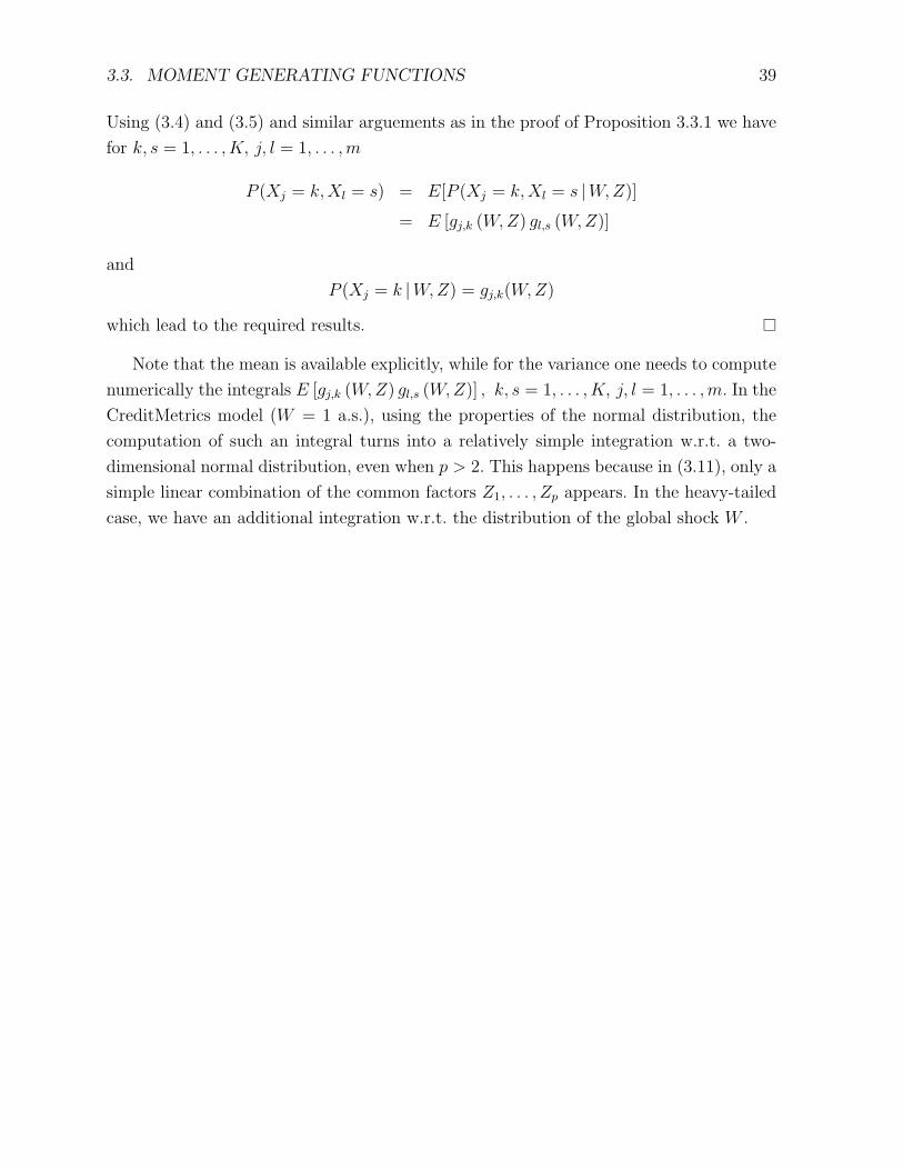
3.3. MOMENT GENERATING FUNCTIONS 39
Using (3.4) and (3.5) and similar arguements as in the proof of Proposition 3.3.1 we have
for k, s = 1, . . . , K, j, l = 1, . . . ,m
P (Xj = k,Xl = s) = E[P (Xj = k,Xl = s |W,Z)]
= E [gj,k (W,Z) gl,s (W,Z)]
and
P (Xj = k |W,Z) = gj,k(W,Z)
which lead to the required results.
Note that the mean is available explicitly, while for the variance one needs to compute
numerically the integrals E [gj,k (W,Z) gl,s (W,Z)] , k, s = 1, . . . , K, j, l = 1, . . . ,m. In the
CreditMetrics model (W = 1 a.s.), using the properties of the normal distribution, the
computation of such an integral turns into a relatively simple integration w.r.t. a two-
dimensional normal distribution, even when p > 2. This happens because in (3.11), only a
simple linear combination of the common factors Z1, . . . , Zp appears. In the heavy-tailed
case, we have an additional integration w.r.t. the distribution of the global shock W .
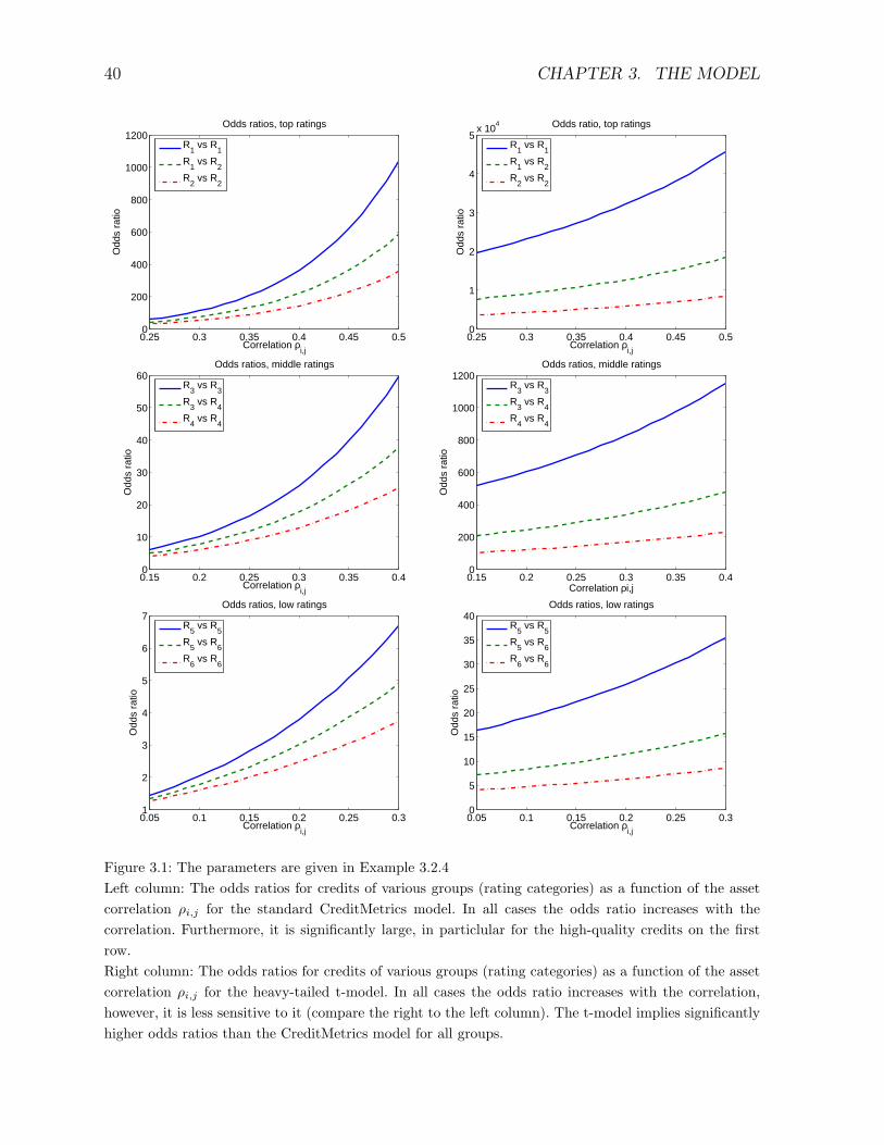
40 CHAPTER 3. THE MODEL
0.25 0.3 0.35 0.4 0.45 0.50
200
400
600
800
1000
1200
Correlation ρi,j
Odd
s ra
tioOdds ratios, top ratings
R1 vs R
1
R1 vs R
2
R2 vs R
2
0.25 0.3 0.35 0.4 0.45 0.50
1
2
3
4
5x 10
4 Odds ratio, top ratings
Correlation ρi,j
Odd
s ra
tio
R1 vs R
1
R1 vs R
2
R2 vs R
2
0.15 0.2 0.25 0.3 0.35 0.40
10
20
30
40
50
60Odds ratios, middle ratings
Correlation ρi,j
Odd
s ra
tio
R3 vs R
3
R3 vs R
4
R4 vs R
4
0.15 0.2 0.25 0.3 0.35 0.40
200
400
600
800
1000
1200Odds ratios, middle ratings
Correlation ρi,j
Odd
s ra
tio
R3 vs R
3
R3 vs R
4
R4 vs R
4
0.05 0.1 0.15 0.2 0.25 0.31
2
3
4
5
6
7Odds ratios, low ratings
Correlation ρi,j
Odd
s ra
tio
R5 vs R
5
R5 vs R
6
R6 vs R
6
0.05 0.1 0.15 0.2 0.25 0.30
5
10
15
20
25
30
35
40Odds ratios, low ratings
Correlation ρi,j
Odd
s ra
tio
R5 vs R
5
R5 vs R
6
R6 vs R
6
Figure 3.1: The parameters are given in Example 3.2.4Left column: The odds ratios for credits of various groups (rating categories) as a function of the assetcorrelation ρi,j for the standard CreditMetrics model. In all cases the odds ratio increases with thecorrelation. Furthermore, it is significantly large, in particlular for the high-quality credits on the firstrow.Right column: The odds ratios for credits of various groups (rating categories) as a function of the assetcorrelation ρi,j for the heavy-tailed t-model. In all cases the odds ratio increases with the correlation,however, it is less sensitive to it (compare the right to the left column). The t-model implies significantlyhigher odds ratios than the CreditMetrics model for all groups.
3.3. MOMENT GENERATING FUNCTIONS 41
0.25 0.3 0.35 0.4 0.45 0.50.5
1
1.5
2
2.5
3
3.5
4
4.5
5x 10
4
Correlation ρi,j
Odd
s ra
tio
Approximation of odds ratios
R1 vs R
1
R1 vs R
1 approx.
R1 vs R
2
R1 vs R
2 approx.
0.15 0.2 0.25 0.3 0.35 0.40
200
400
600
800
1000
1200Approximation of odds ratios
Correlation ρi,j
Odd
s ra
tio
R3 vs R
3
R3 vs R
3 approx.
R4 vs R
4
R4 vs R
5 approx.
0.05 0.1 0.15 0.2 0.25 0.30
5
10
15
20
25
30
35
40Approximation of odds ratios
Correlation ρi,j
Odd
s ra
tio
R5 vs R
5
R5 vs R
5 approx.
R6 vs R
6
R6 vs R
6 approx.
Figure 3.2: The parameters are given in Example 3.2.5 (the same as in Figure 3.1)The odds ratios for credits of various rating categories as a function of the asset correlation ρi,j forthe t-model, compared to the approximation using tail dependence. The approximation is accurate, inparticular for the high quality credits in the left plot.

42 CHAPTER 3. THE MODEL
Chapter 4
Calibration
The practical implementation of any portfolio credit risk model depends crucially on the
effectiveness of the statistical procedures for estimation of the model parameters. In model
(3.1) with (3.4) and (3.5) the parameter space includes:
(1) the marginal distributions of the ratings Xj, j = 1, . . . ,m;
(2) the marginal distributions of the losses Lj, given Xj, j = 1, . . . ,m;
(3) the copula of the assets Y (see Proposition 3.1.1). By means of (3.5), this copula
is determined by the distribution of the global shock W , the correlation matrix Σ of the
common factors Z1, . . . , Zp and the factor loadings αj,l, σj, j = 1, . . . ,m, l = 1, . . . , p.
In the next section we describe briefly the available approaches regarding the one-
dimensional marginal parameters (1) and (2). We continue with the bivariate case and in
Section 4.2 we introduce several estimation methods for important dependence measures
for two-dimensional random vectors, including the linear correlation, Kendall’s tau and
the tail dependence coefficients. Particular attention is paid to the estimation of the tail
dependence coefficient, where a new method aiming at a lower variance of the estimates is
suggested. In Section 4.3 we consider the calibration of a multidimensional elliptical cop-
ula, based on i.i.d. observations of a random vector with arbitrary continuous marginals.
We start with several semi-parametric and non-parametric methods for dealing with the
marginals of the observed random vector. We continue with two classical methods for cop-
ula estimation. The main result in this section is a new calibration procedure for an ellip-
tical copula, which makes extensive use of the information contained in the joint extreme
observations. In Section 4.4 we apply the procedure to calibrate model (3.5). An additional
result regarding the estimation of the factor loadings αj,l, σj, j = 1, . . . ,m, l = 1, . . . , p in
(3.5) is provided. We conclude this chapter with an extended simulation study and some
real data examples.
43
44 CHAPTER 4. CALIBRATION
4.1 Marginal parameters
4.1.1 Rating migration probabilities
The possibility that major rating agencies will change the credit rating of an obligor is
an important source of credit risk, above and beyond its implications for the direct risk
of default. Changes in the credit ratings may have an immediate effect on the values of
defaultable bonds portfolios, may indicate that certain credits are no longer admissible
for investors, who are subject to restrictions on the ratings of their credits, and may lead
even to mandatory termination of some financial contracts. Some corporate bonds have
coupon rates linked explicitly to the credit rating. The BIS capital accord determines the
capital requirements of the regulated banks based in part on the credit ratings of the
obligors they have in their portfolios. For these and related reasons, a model for the risk
of a rating change is a key ingredient of the credit risk management system.
In what follows we model the credit rating of an obligor as a continuous-time stochastic
process (X(t))t≥0 with state space 1, . . . , K, where state 1 means default (absorbing
state), and the credit quality increases with the rating. This numeric notion is chosen
only for notational convenience; if we use e.g. Moody’s rating categories, we would set
K = 8, X = 8 corresponding to rating Aaa, X = 7 to Aa and so on until X = 2 Caa and
X = 1 default (D).
Furthermore, we assume that the rating process follows the dynamics
dX(t) = (VX(t) −X(t))dNX(t)(t) , t ≥ 0 ,
where N = (N1, . . . , NK) is a set of independent time-homogeneous Poisson processes with
intensities λ1, . . . , λK and V1, . . . , VK is a set of mutually independent and independent of
N discrete r.v.s with d.f.s, for k = 1, . . . , K,
P (Vk = j) =λkjλk
j = 1, . . . , K, j 6= k ,
with λkj being some positive constants summing up to λk.
Under these assumptions, the credit rating processX(t) is a time-homogeneous Markov
process, see e.g. Schonbucher [129], Section 8.2.3. More precisely, we have that for all T > t
P (X(T ) = j | Ft) = P (X(T ) = j |X(t)) , j = 1, . . . , K , (4.1)
and, denoting by Q(t, T ) = [qkj(t, T ) = P (X(T ) = j |X(t) = k)]k,j=1,...,K , we have also
Q(t, T ) = Q(T − t, 0) := Q(T − t) . (4.2)
In particular, Q(t) = exp(Λt), t ≥ 0, where Λ = [λjk]j,k=1,...,K with λkk = −λk, k =
1, . . . , K. The matrix Λ is often called generator matrix. It describes completely the
stochastic behaviour of the rating process X.
4.1. MARGINAL PARAMETERS 45
The calibration of the generator matrix Λ is complicated by the fact that usually
the rating agencies publish only rating migrations over a given time period like 1 year.
The most common method for estimation in this case is based upon the observed be-
haviour of groups of obligors within the same initial rating, the cohorts. Denote by
nk(t), k = 1, . . . , K, the total number of obligors of rating k at time t, and by nkj(t1, t2)
the number of observed migrations of obligors with rating k at time t1 to rating j at time
t2 > t1. Due to the Markov chain dynamics of the rating process, these migration events
can be viewed as outcomes of nk(t1) independent multinomial trials. With rating migra-
tion observations over T periods, the maximum likelihood estimator for the one-period
migration probabilities qkj(1) is
qkj(1) =1
T
T∑t=1
nkj(t− 1, t)
nk(t− 1),
see e.g. Johnson and Kotz [84], Chapter 3 for confidence intervals.
This standard estimator has certain weak points. First, it does not utilize the full
continuous-time information on the rating migrations which could be available at a rating
agency or at a bank. In particular, when it comes to the rare events like a default of a
high-rated obligor, the method usually produces 0 as an estimate. This is due to the fact
that in practice a default of such an obligor typically happens not immediately within
one period, but through a sequence of rating downgrades. This information cannot be
captured by the standard estimator.
In addition, estimating a one-period migration probability matrix Q(1) by Q(1) does
not automatically imply an estimate Λ for the generator matrix Λ. Israel et al. [79] consider
the problem of finding a generator matrix Λ consistent with Q(1). It is well-known that for
certain stochastic matrices Q, there exists no generator matrix. Israel et al. [79] provide
sufficient conditions on Q(1) for the existence of a generator. Furthermore, there can be
distinctly different generator matrices consistent with the same migration matrix Q(1),
implying different estimates for migration probabilities Q(t), for all t 6= 1. The problem is
known as embedding problem for continuous-time Markov chains. It is studied in detail by
Kreinin and Sidelnikova [95], who give also a survey on the available numerical methods
for it.
To avoid these problems, Lando and Skodeberg [98] propose a direct maximum like-
lihood estimator for the generator matrix. It requires knowledge of the precise points in
time (the exact dates) at which rating migrations take place.
For k, j = 1, . . . , K, denote by mkj(t) the total number of migrations from rating k to
rating j throughout the period [0, t]. Recall the notation nk(t) as above. Then a maximum
46 CHAPTER 4. CALIBRATION
likelihood estimator for the migration intensities in the generator matrix Λ is
λkj =mkj(T )∫ T0nk(t)dt
, k, j = 1, . . . , K ,
see Lando and Skodeberg [98] for asymptotic properties and confidence bounds.
To conclude this section, we note that with respect to the rating modelling, the time-
homogeneos Markov chain assumptions are quite strong and cannot be confirmed by
empirical data. The default and migration probabilities vary significantly with the busi-
ness cycle, as documented by Nickell et al. [120] and Kavvathas [87]. This contradicts to
the time-homogenuity assumption (4.2). In addition, Behar and Nagpal [12], Lando and
Skodeberg [98], and Kavvathas [87] all find that, for obligors of certain ratings, the prior
rating is an important determinant of the likelihood of a downgrade (and default) v.s
that of an upgrade, over a given time horizon. There is indeed an apparent momentum in
rating migration data, which contradicts to (4.1). Also, there is a significant aging effect
(dependence of the migration probabilities on the duration in a rating category and/or the
age of the credit), documented by Carty and Fons [20], Lando and Skodeberg [98], and
Kavvathas [87]. Further information for the obligors available from the rating agencies
like watch-lists and outlooks could also be important for accurate estimation of the de-
fault and migration probabilities, see Cantor and Hamilton [19]. To summarize, different
obligors of the same rating have different default and migration probabilities, and a given
obligor of a fixed rating has default and migration probabilities which change over time.
For this reason, in the thesis we consider the marginal default and migration probabilities
in (3.2) as attributes of the individual credit and not of the rating category to which the
credit belongs. This gives a sufficient flexibility to the model and allows for statistical
estimation of the credit risk based on every kind of relevant information for the marginal
credits that could be available.
4.1.2 Loss given rating
Knowing the credit quality (the rating) of a given obligor at the time horizon is not
sufficient in itself to determine completely the profit/loss, which the bank will generate
for holding the credit. In case of default, it is not clear whether the collateral of the credit
will be sufficient to cover at least the expected part of the losses. In all other cases, the
change in the market value of the credit may not be completely determined by the credit
rating.
An important ingredient of any credit risk model is the loss given default (LGD), i.e.
the d.f. of Lj, given Xj = 1, for j = 1, . . . ,m in (3.1). Gupton and Stein [75] and Hamilton
et al. [76] provide comprehensive studies and point out the most powerful determinants
of LGD. Their key findings are:
4.2. BIVARIATE DEPENDENCE MEASURES 47
- The type of the obligor and the type of the credit are the most powerful determinants.
- The initial rating category of the obligor can also be used as a predictor: the higher
the rating, the lower the LGD.
- The LGD moves with the business cycle and thus is positively correlated with the
default probabilities: the higher the default probabilities, the higher the LGD.
These and some additional factors are summarized in Moody’s Loss-Calc – the indus-
trial model for prediction of LGD, see Gupton and Stein [75]. Further studies of historical
LGD are Eberhart and Sweeny [44], Altman [3], Altman and Kishore [4] and many others.
Apart from the case of default, a lot of research has also been done in the development
of rating-based forward pricing models for single-obligor credit risks (bonds and deriva-
tives). A general pricing framework can be found in Lando [97]. Jarrow et al. [81] consider
a very simple case leading to deterministic prices, given the rating. CreditMetrics [74]
takes also a similar approach. More complicated, but more realistic, are the models de-
veloped for instance by Das and Tufano [28], and Li [103]. We do not go into detail since
our goal is the portfolio view of credit risk. We adopt a general formulation. In this thesis
the profit/loss of the individual credit, given its credit rating, is modelled by an arbitrary
r.v. Lj, see model (3.1). Specifying the distribution of this r.v., for all possible rating
categories at the risk horizon, and the corresponding default and migration probabilities
as in Section 4.1.1 is sufficient to calibrate the marginal loss distribution in our model.
More problematic are assumptions (A) and (B) in model (3.1). Sytematic dependen-
cies between the losses given rating are observed in various empirical studies, see e.g.
Frye [63, 64]. In particular, for some credit types LGDs are positively correlated with
certain market factors. The effect of this dependence on the portfolio level is studied by
Oda and Muranaga [121] and by Frey and McNeil [61], Section 5.1 (systematic recovery
risk). For the sake of simplicity, we disregard this dependence and keep assumptions (A)
and (B).
4.2 Bivariate dependence measures
We focus on the dependence structure of a two-dimensional random vector (Y1, Y2) with
continuous marginals. Throughout this section we assume that we are given a sample
(Y(i)
1 , Y(i)
2 ), i = 1, . . . , n, of i.i.d. copies of (Y1, Y2).
In Section 4.2.1 we consider the estimation of some classical dependence measures for
the whole range of Y1 and Y2. In Section 4.2.2 we consider the estimation of the tail
dependence coefficient which measures the dependence in the extremes of Y1 and Y2.
48 CHAPTER 4. CALIBRATION
4.2.1 Kendall’s tau and correlation
Recall Definition 2.1.6 of the linear correlation coefficient. Given a sample (Y(i)
1 , Y(i)
2 ), i =
1, . . . , n, of i.i.d. copies of the random vector (Y1, Y2) with finite variances, it is straight-
forward to estimate the variance of Yj, j = 1, 2, by
σ(Yj) =1
n− 1
n∑i=1
(Y(i)j − Y j,n)2 ,
where
Y j,n =1
n
n∑i=1
Y (i) .
In order to estimate the linear correlation coefficient, we may compute the sample covari-
ance
cov(Y1, Y2) =1
n− 1
n∑i=1
(Y(i)
1 − Y 1,n)(Y(i)
2 − Y 2,n) ,
and then use
ρ(Y1, Y2) =cov(Y1, Y2)√σ(Y1)
√σ(Y2)
. (4.3)
This estimator is classical and works quite satisfactory in the case when (Y1, Y2) are
bivariate normal. However, it has certain weak points. In particular, it depends crucially on
the marginals of Y1 and Y2. When they are asymmetric or heavy-tailed, the estimator lacks
robustness. For instance, when var(Y1) =∞, it may not even converge. Recall that (2.14)
provides a definition of the correlation coefficient in the framework of elliptical copulas,
which does not rely on marginal assumptions, and in particular allows for marginal heavy-
tails and infinite variances. Since model (3.5) is essentially based on elliptical copulas
and does not exclude heavy-tailed marginals, we need an alternative method to estimate
ρ(Y1, Y2).
Various covariance and correlation estimators have been proposed including M-estimators,
estimators based on multivariate trimming and estimators based on variances of sums and
differences of standardized variables (see Devlin et al. [35] for an overview). Particularly
useful in the framework of elliptical distributions are the methods suggested by Frahm
and Junker [57] and by Lindskog et al. [104].
The estimator of Frahm and Junker [57] is in principle applicable to a random vec-
tor Y of arbitrary dimension d ≥ 2 with elliptical distribution. It uses extensively the
repesentation of such a random vector Y = RAU + µ as in (2.13). First one needs to
estimate the mean vector µ ∈ Rd. This can be done easily by the sample mean vector
(Y 1,n, . . . , Y d,n). Alternatively, under some technical conditions detailed in Bunning and
Trenkel [18], Chapter 3, the sample median vector is also a consistent estimate for µ (re-
call that the marginals of the elliptical distributions are symmetric). Once we have an
4.2. BIVARIATE DEPENDENCE MEASURES 49
estimate for µ, we substract it from the data and assume that we have Y = RAU in
(2.13). Denote by | · | the L2 norm on Rd. We have that
S :=Y
|Y |d=
AU
|AU |.
The vector S is distributed on the unit hypersphere (since U is), and, given the matrix
A, its density can be computed explicitly. In order to estimate A, one maximizes the
likelihood function
Γ = arg maxΓ
log(L(A;S(1), . . . , S(n))) = arg maxΓ
n log(det(Γ′Γ))− d∑i=1
nS(i)Γ′ΓS(i) ,
where S(1), . . . , S(n) are the observed i.i.d. copies of S and Γ = δA−1 with δ > 0 being
a design constant, see Frahm and Junker [57] for more details. Once the estimate Γ is
available, we get directly an estimate for the correlation coefficients as defined in (2.14)
(recall that Σ = A′A and that the correlation is invariant under scaling with a constant
δ).
In contrast to the above method, the estimator suggested in Lindskog et al. [104] is
applicable to the more general situation when Y is a random vector with arbitrary abso-
lutely continuous marginals and elliptical copula. It is essentially based on Theorem 2.3.11
which shows that the elegant relationship
ρ(Y1, Y2) = sin(π
2τ(Y1, Y2)) (4.4)
between the linear correlation coefficent defined in (2.14) and Kendall’s tau defined in (2.1)
holds when (Y1, Y2) have an elliptical distribution with absolutely continuous marginals.
The result is not only of theoretical interest; it is also extremely useful for statistical
purposes. It can be used to build a robust estimator of the linear correlation coefficient
for data coming from a distribution with elliptical copula. Formula (4.4) provides an
appealing bivariate method; we estimate the Kendall’s tau using the standard textbook
estimator and then plug it in relationship (4.4) to get the Kendall’s tau transform estimate
of ρ. More precisely, one may consistently estimate the Kendall’s tau by
τ(Y1, Y2) =
(n
2
)−1 n∑i>k
sign[(Y(k)
1 − Y (i)1 )(Y
(k)2 − Y (i)
2 )], , (4.5)
and then use
ρ(Y1, Y2) = sin(π
2τ(Y1, Y2)) . (4.6)
The estimator (4.5) is consistent and asymptotically normal, see e.g. Hoffding [77], which
implies the same for the correlation estimate (4.6) by the continuous mapping theorem
and the delta method. Simulation studies in Lindskog et al. [104] suggest that this simple
50 CHAPTER 4. CALIBRATION
method performs better than most of its competitors. Further results in Daul et al. [30]
show that (4.4) provides also a quite accurate approximation of the correlation coefficient
in more general situations than an elliptical copula, hence (4.6) is also quite robust. We
present some examples in Section 4.5, which investigate the accuracy of the estimator for
modest sample size.
Note that, unlike other methods of correlation estimation, the Kendall’s tau transform
method directly exploits the geometry of the elliptical distributions and does not require
to estimate variances and covariances. This is advantageous when the interest focusses
explicitly on correlations, as it often does in financial applications, and in particular in
our credit risk model. Recall that by means of Proposition 3.1.1 the copula of the assets
Y determines the distribution of the ratings X (which is of central interest in our work)
regardless of the assets’ marginals, and that the correlations ρ(Yi, Yj), i, j = 1, . . . ,m, are
essential parameters of this copula.
More generally, (4.6) can be used to calibrate the correlation matrices of higher di-
mensional elliptical copulas. However, in some cases the matrix of the pairwise correlation
estimates has to be adjusted numerically to ensure that the resulting matrix is positive
definite; see Rousseeuw and Molenberghs [125] for details. Note that the factor model
(3.5) guarantees that the (high-dimensional) correlation matrix ΣY ∈ Rm×m of the assets
is positive definite as long as (the lower-dimensional) correlation matrix of the common
factors Σ ∈ Rp×p is. This reduces the problem significantly, and in most practical cases no
or just minor adjustments of the correlation matrices are necessary (see Schwarz [131]).
4.2.2 Tail dependence
Recall Definition 2.1.12 of the tail dependence coefficient. In this section, we consider sev-
eral methods for estimating this dependence measure, based on a sample (Y(i)
1 , Y(i)
2 ), i =
1, . . . , n, of i.i.d copies of the random vector (Y1, Y2). We focus on the lower tail dependence
coefficient; the same methods can be applied to the upper tail dependence, by considering
the vector (−Y1,−Y2). We assume also that (Y1, Y2) are tail-dependent. Statistical meth-
ods for testing of tail dependence or tail independence go beyond the scope of this work,
for that we refer the reader to Ledford and Tawn [99] and Draisma et al. [36].
The main difficulty in estimating tail dependence arises in the limited availability of
extreme data. According to the assumptions on the distribution of the observed random
vector, the methods for estimating the tail dependence can be classified as parametric,
semi-parametric and non-parametric methods. According to the usage of data, the ap-
proaches are ascribed either to the entire dataset or to a subset of extreme data.
Within the framework of the methods based on extreme data, the extreme value theory
introduced in Section 2.2.1 contains the natural tools for inferences on the tail behavior
4.2. BIVARIATE DEPENDENCE MEASURES 51
of (one-dimensional) probability distributions. In the one-dimensional setting the class of
extreme value distributions has a finite parametrization, so it suffices to apply paramet-
ric estimation methods. By contrast, no finite parametrization of the multidimensional
extreme-value distributions exists. This leads to more complicated estimation methods.
A key result in this section is a new non-parametric estimator of the tail dependence
coefficient which utilizes only the extreme observations. We start with some classical
methods.
(A) Parametric tail dependence estimators based on the whole available
sample.
In this class of methods, the d.f. of the vector (Y1, Y2) is assumed to belong to a certain
parametric family. Classical methods like maximum likelihood (ML) provide estimators
for the parameters of the entire d.f. An estimator of the tail dependence coefficient in this
case follows as a by-product. Under the usual regularity conditions for the ML theory (see
e.g. Casella and Berger [21], p.516), this tail dependence estimator can be shown to be
consistent and asymptotically normal. However, recall from Proposition 3.1.1 that in our
credit risk application we are interested in the copula of a random vector, rather than in
its full d.f. Since the tail dependence coefficient itself is essentially a copula property, it
would be more natural to estimate it without making assumptions on the marginals. The
next method (B) is a step in this directlion.
(B) Semi-parametric tail dependence estimators based on the whole avail-
able sample.
In this class of methods, the copula of the vector (Y1, Y2) is assumed to belong to a cer-
tain parametric family, and the marginals are left arbitrary (but continuous, so that the
copula of the random vector is uniquely determined, see Theorem 2.1.2). In this case a
two-step method can be applied. In the first step, one has to transform the marginals Y1
and Y2 into uniform r.v.s, using one of the methods described in Section 4.3.1. In the sec-
ond step, one estimates the parameters of the copula, using for instance the ML methods
described in Section 4.3.2. As in method (A), an estimator of the tail dependence follows
as a by-product from the parameric copula assumptions. Genest et al. [65] show that such
estimators are consistent and asymptotically normal.
The main drawback of the above approaches (A) and (B) is that they infer the tail
dependence coefficient, which is a measure for the dependence in the extremes, without
putting more weight on the extreme observations. The methods that follow focus on this
issue.
(C) Tail dependence estimator for elliptically distributed vector, which uti-
lizes the extreme observations.
Recall from Proposition 2.3.12 that the tail dependence coefficient of a bivariate elliptical
52 CHAPTER 4. CALIBRATION
random vector with represenation Y = RAU + µ as in (2.13) is given by:
λ(Y1, Y2) =
∫ π2
g(ρ1,2) cosα t dt∫ π2
0cosα t dt
,
where g(t) = π4− arcsin t
2, t ∈ (−1, 1) and α is the tail index of the regularly varying r.v. R.
Therefore, it is sufficient to estimate the correlation coefficient ρ1,2 and the tail index α of
the spectral variable R. The estimation of the correlation ρ1,2 can be done by one of the
methods applicable to heavy-tailed elliptical distributions described in Section 4.2.1. For
the estimation of the tail index α we note that by Proposition 2.2.15 the r.v. |Y | (| · | being
an arbitrary norm) is regularly varying with the same tail index as the random vector
Y . Therefore it is sufficient to apply standard one-dimensional extreme value theory to
estimate the tail index of |Y |. Kluppelberg et al. [91] apply the Hill estimator (2.8) and
prove consistency and asymptotic normality of the resulting tail dependence estimator.
Alternatively, Frahm et al. [58] apply the POT method (end of Section 2.2.1). In both
cases | · | is taken to be the L2-norm, althought theoretically this is not a significant
requirement.
An advantage of the approach (C) is that it utilizes the extreme observations by
applying the Hill estimator or the POT method in the estimation of the tail index α of
the elliptical random vector. However, there are certain drawbacks which are similar to the
drawback of approach (A). The marginal tails in fact play a crucial role in the estimation
of the tail index α, and hence in the estimation of the tail dependence. The method
cannot be applied to distributions with elliptical copula and arbitrary marginals, which
are of central interest in our credit risk model. In many practical applications one can find
that whereas the elliptical copula is a reasonable model for the dependence structure of
the financial assets under consideration, they exhibit a different marginal behaviour, and
in particular do not have heavy tails, see Example 4.5.5 or Schwarz [131]. In such cases
method (C) breaks down.
Parametric estimation methods have the advantage of being efficient given that the
model is true whereas nonparametric estimation avoids model-misspecification. The next
methods are non-parametric, and are based on the extreme observations. We start with a
method based on the assumption that the random vector under consideration is a general
regularly varying vector.
(D) Tail dependence estimator for regularly varying random vectors.
Let (Y1, Y2) be a regularly varying random vector with tail index α and continuous
marginals G1 and G2 resp. Recall the estimator of the spectral measure µ as in (2.12). Of
particular interest in the context of tail dependence are probabilities like
π(p, q) = P (Y1 > G−11 (1− p) |Y2 > G−1
2 (1− q)) ,
4.2. BIVARIATE DEPENDENCE MEASURES 53
where p and q are some small probabilities. The key idea is to use the scaling property
of the Radon measure µ as in Proposition 2.2.16. Making use of (2.11), Wendin [135]
suggests to approximate the spill-over probability π(p, q), for p, q being small, by
π(p, q) =µ((s, t) : s > (q/
√q2 + p2)1/α , t > (p/
√q2 + p2)1/α)
µ((s, t) : s > (q/√q2 + p2)1/α)
. (4.7)
Invoking the estimator µ as in (2.12) one obtains the corresponding estimator π(p, q) for
π(p, q), i.e.
π(p, q) =µn((s, t) : s > (q/
√q2 + p2)1/α , t > (p/
√q2 + p2)1/α)
µn((s, t) : s > (q/√q2 + p2)1/α)
Setting p = q in (4.7) and making use of the scaling property of the Radon measure µ as
in Proposition 2.2.16 we obtain an estimator for the upper tail dependence coefficient
λµ =µn((s, t) : s > 1/
√2 , t > 1/
√2)
µn((s, t) : s > 1/√
2)(4.8)
where µn is the estimator of the Radon measure given in (2.12). Note that, unlike the
estimator presented in (C), (4.8) does not depend on the tail index α. However, it is still
based on the assumption that the marginal distributions are regularly varying with the
same tail index α as the vector, see e.g. the conlcusion in Wendin [135]. Similarly to the
method (C), the method (D) is not applicable to the more general case of a tail dependent
random vector with arbitrary marginals.
The next methods which we consider are completely non-parametric, and in particular
nothing more than continuity is assumed for the marginals.
(E) Empirical tail dependence estimator.
Let Y = (Y1, Y2) be a bivariate random vector with continuous marginals, copula C and
tail dependence λ(Y1, Y2). Let Y (i), i = 1, . . . , n, be i.i.d. copies of Y . Theorem 2.1.2
suggests an estimate of C(p, p), for p ∈ (0, 1):
CE(p, p) =1
n
n∑i=1
1FE1 (Y(i)1 )<p , FE2 (Y
(i)2 )<p , (4.9)
where FEj (p) denotes the empirical d.f. of Yj, for j = 1, 2. Invoking an auxiliary sequence
k = k(n) with the properties k →∞ and kn→ 0 as n→∞ we obtain
λn,k =n
kCE(
k
n,k
n)P→ λ(Y1, Y2) , n→∞ , (4.10)
see Schmidt and Stadtmuller [127] for a proof of the above fact and for asymptotic nor-
mality of the suggested estimator.
54 CHAPTER 4. CALIBRATION
The main drawback of the above approach is in the high variance of the simple em-
pirical estimation of rare event probabilities. The next method is expected to perform
better.
(F) Log-transform method.
Let Y be a tail-dependent bivariate random vector with continuous marginals and a
differentiable copula C. Then for its tail dependence coefficient we have
λ(Y1, Y2) = limu→0
C(u, u)
u= 2− lim
u→0
log(1− 2u− C(u, u))
log(1− u).
Recall that 1−2u+C(u, u) = C(1−u, 1−u) by definition. Invoking the empirical copula
estimator (4.9) and an auxiliary sequence k = k(n) with the properties k →∞ and kn→ 0
as n→∞ we obtain
2−logCE(1− k
n, 1− k
n)
log(1− kn)
P→ λ(Y1, Y2) , n→∞ , (4.11)
see Coles et al. [22] for a proof and for asymptotic properties of the estimator.
We conclude with a new tail dependence estimator, which combines ideas from meth-
ods (D), (E) and (F).
(G) Alternative tail dependence estimator.
Let Y be a tail-dependent bivariate random vector with continuous marginals, differen-
tiable copula C and tail dependence coefficient λ(Y1, Y2). Let Y (i), i = 1 . . . , n, be i.i.d.
copies of Y . We start by noting that the weakest point of the tail dependence estimator
(4.10) is that it is a simple empirical estimator based on the extreme observations. More
precisely, denote
U(i)j = FE
j (Y(i)j ), j = 1, 2, i = 1, . . . , n , (4.12)
where FEj is the empirical d.f. of Yj. Then the estimator in (E) can be rewritten as
λn,u =1
n
n∑i=1
1
u1U(i)
1 <u,U(i)2 <u ,
where u ∈ (0, 1) is some small threshold. We consider the extremes in a different set
and use a weighted empirical estimator with weights proportional to the distance to the
diagonal U1 = U2. To this end, we transform further (U(i)1 , U
(i)2 ), i = 1, . . . , n, into polar
coordinates
U(i)1 = Q(i) sinφ(i), U
(i)2 = Q(i) cosφ(i), i = 1, . . . , n, (4.13)
where the r.v.s (Q(i), φ(i)) satisfy 0 ≤ Q(i) ≤√
2 and 0 ≤ φ(i) ≤ π2. Then we select a small
r ∈ (0,√
2) and we suggest the following estimator
λn,r =1
n
n∑i=1
√2
r1Q(i)<r sin(2φ(i)). (4.14)
In the following proposition we prove consistency of the suggested estimator.
4.2. BIVARIATE DEPENDENCE MEASURES 55
Proposition 4.2.1. For n ∈ N let Y (i) = (Y(i)
1 , Y(i)
2 ), i = 1, . . . , n, be a sequence of i.i.d
random vectors with differentiable copula C and arbitrary continuous marginals F1, F2.
Let also (Q(i), φ(i)), i = 1, . . . , n, be the r.v.s in (4.13). Let k = k(n) be a sequence of
positive constants such that k(n)→∞ and k(n)n→ 0, n→∞. Then
λn, k/nP→ λ∗, n→∞ , (4.15)
where λ∗ is the tail dependence coefficient of (Y1, Y2).
Proof. Denote by
U(i)
j = Fj(Y(k)j ), j = 1, 2, i = 1, . . . , n ,
where Fj is the true d.f. of Yj, and the corresponding (Q(i), φ
(i))i=1,...,n as in (4.13) and
note that this is an i.i.d sequence, since (Y(i)
1 , Y(i)
2 )i=1,...,n is an i.i.d. sequence. Denote also
by λn,k/n
the corresponding r.v. as in (4.14). Since Fj, j = 1, 2, is a monotone function, we
have for the copula CU
(i)1 ,U
(i)2
= C, i = 1, . . . , n. Fix i ∈ 1, . . . , n and denote Q = Q(i)
,
φ = φ(i)
, Uj = U(i)
j , j = 1, 2. We have
1Q<r sin(2φ) = 1Q<r2 sinφ cosφ
= 1Q<r2(Q sinφ)(Q cosφ)
Q2
d= 1
√U2
1 +U22<r
2U1U2
U21 + U2
2
.
Therefore
E[1Q<r sin(2φ)] =
∫ ∫D=√u2
1+u22<r
2u1u2
u21 + u2
2
dC(u1, u2).
Changing variables by z =√u2
1 + u22 ∈ (0, r), t =
√2u1u2 ∈ (0, z) we obtain
E[1Q<r sin(2φ)] =
∫ r
0
∫ z
0
t2
z2dC
(√z2 + t2 +
√z2 − t2
2,
√z2 + t2 −
√z2 − t2
2
)
Therefore, applying L’Hopital’s rule
limr→0
√2
rE[1Q<r sin(2φ)] = lim
r→0
∂
∂u1
C(u1, u2)|u1=u2=r + limr→0
∂
∂u2
C(u1, u2)|u1=u2=r . (4.16)
However, by definition,
λ∗ = limu→0
C(u, u)
u= lim
r→0
∂
∂u1
C(u1, u2)|u1=u2=r + limr→0
∂
∂u2
C(u1, u2)|u1=u2=r.
56 CHAPTER 4. CALIBRATION
Then (4.15) follows from Chebishev’s inequality. More precisely, we have for every ε > 0,
P(∣∣∣λn,k/n − λ∗∣∣∣ > ε
)≤ 1
ε
(E∣∣∣λn,k/n − λn,k/n∣∣∣+ E
∣∣∣λn,k/n − Eλn,k/n∣∣∣+∣∣∣Eλn,k/n − λ∗∣∣∣) .
From (4.16) we have that Eλn,k/n → λ∗, n→∞.
By the SLLN we have λn,k/n a.s.→ Eλ
n,k/n, n→∞.
Finally, since FEj (Y (i))
a.s.→ Fj(Y(i)) we have also
(Q(i), φ(i))a.s.→ (Q
(i), φ
(i)), i = 1, . . . , n . (4.17)
Furthermore
E∣∣∣λn,k/n − λn,k/n∣∣∣ ≤ √
2
k/nE∣∣∣1Q(i)<r sin(2φ(i))− 1Q(i)
<r sin(2φ(i)
)∣∣∣
≤√
2
k/nE∣∣∣1Q(i)<r − 1Q(i)
<r
∣∣∣≤√
2
k/n
(P (Q(i) <
k
n)P (Q(i) −Q(i)
< 0) + P (Q(i)<k
n)P (Q(i) −Q(i)
> 0)
)However, similarly as above,
P (Q(i)< r) =
∫ r
0
∫ z
0
dC
(√z2 + t2 +
√z2 − t2
2,
√z2 + t2 −
√z2 − t2
2
)
and, applying L’Hopital’s rule,√
2rP (Q
(i)< r) → λ∗ < ∞ as r → 0. By (4.17) we obtain
also√
2rP (Q(i) < r)→ λ∗ <∞ and P (|Q(i) −Q(i)| 6= 0)→ 0 as n→∞. This leads to the
required result.
Note that the estimators in (E), (F) and (G) may not necessarily be applied by using
the empirical d.f. to transform the data to the copula scale as suggested in (4.12). One may
potentially replace the empirical d.f. FEj , j = 1, 2, in that equation by another consistent
estimate, see Section 4.3.1. However, this will presumably have a small impact on the
estimators in (E) and (D), as they are based essentially on a direct approximation of the
copula function at a single point, i.e. C(k/n, k/n) is approximated by e.g. CE(k/n, k/n)
in (4.10) and C(1− k/n, 1− k/n) by e.g. CE(1− k/n, 1− k/n) in (4.11). In contrast to
that, the new estimator (4.14) is intended to capture more information from the joint
extreme observation by assigning different weights to each one of them. Consequently,
replacing the empirical d.f. in (4.12) by another consistent estimate of the marginal d.f.
(which is advisable e.g. when we are dealing with marginal heavy tails) will have a direct
impact on the weights and thus on the tail dependence estimate.
In the next proposition we show asymptotic normality of the suggested estimator
(4.14), provided the marginal d.f.s are known. Since (4.14) is just a weighted estimator,
4.2. BIVARIATE DEPENDENCE MEASURES 57
the asymptotic variance is the same as the variance of the empirical estimator (E), see
Schmidt and Stadtmuller [127], Theorem 5.
For n ∈ N let Y (i) = (Y(i)
1 , Y(i)
2 ), i = 1, . . . , n, be a sequence of i.i.d random vectors with
differentiable copula C, tail dependence coefficient λ∗ and arbitrary continuous marginals
F1, F2. Assume that there exists a functon A(p) : R+ → R+ such that A(p) → 0, p → 0
andC(p, p)/p− λ∗
A(p)= g <∞ , p→ 0 . (4.18)
Denote by
U(i)
j = Fj(Y(k)j ), j = 1, 2, i = 1, . . . , n ,
and the corresponding (Q(i), φ
(i))i=1,...,n as in (4.13). Denote also by λ
n,k/nthe correspond-
ing r.v. as in (4.14).
Proposition 4.2.2. With the above notations, let k = k(n) be a sequence of positive
constants such that k(n)→∞ and k(n)n→ 0, n→∞. If
√kA(k/n)→ 0 , n→∞ ,
where A is the function in (4.18), then
√k(λ
n,k/n − λ∗) d→ N(0,√
2λ∗) , n→∞ .
Proof. We have
√k(λ
n,k/n − λ∗) =√k(λ
n,k/n − E[λn,k/n
]) +√k(E[λ
n,k/n]− λ∗) .
By (4.16) and (4.18) we get
limn→∞
√k(E[λ
n,k/n]− λ∗) = lim
n→∞
√kgA(k/n) = 0 .
Furthermore,√k(λ
n,k/n − E[λn,k/n
]) =n∑i=1
Zk,n ,
where Z(i)k,n =
√2√k(1Q(i)
<k/n sin(2φ(i)
) − E[1Q(i)<k/n sin(2φ
(i))]). By definition, Z
(i)k,n are
i.i.d. with mean E[Z(i)k,n] = 0, i = 1, . . . , n. Denoting by Zk,n =
√2√k(1Q<k/n sin(2φ) −
E[1Q<k/n sin(2φ)]) a generic r.v. with the same distribution as Z(1)k,n, we have
var(n∑i=1
Z(i)k,n) = nE[Z2
k,n] . (4.19)
58 CHAPTER 4. CALIBRATION
Then we compute
nE[Z2k,n] =
√2n
kE[√
21Q<k/n sin2(2φ)]− k
n
(nkE[√
21Q<k/n sin2(2φ)])2
.
The second term converges to 0 as n tends to infinity because of (4.16):
limn→∞
k
n
(nkE[√
21Q<k/n sin2(2φ)])2
= limn→∞
k
n(λ∗)2 = 0 .
Using the same change of variable as in the proof of Proposition 4.2.1 we get for the first
part
√2n
kE[√
21Q<k/n sin2(2φ)] =√
2n
k
∫ kn
0
∫ z
0
√2t4
z4dC
(√z2 + t2 +
√z2 − t2
2,
√z2 + t2 −
√z2 − t2
2
).
Applying L’Hopital’s rule and going back to (4.19) we obtain
var(n∑i=1
Z(i)k,n)→
√2λ∗ .
Finally we note that |Z(i)k,n| ≤
√2k
a.s. and therefore, for every i = 1, . . . , n,
P (|Z(i)k,n| > ε)→ 0 , n→∞
for every ε > 0. Then the required result then follows from Theorem 4.1. in Petrov [123].
We leave the question for asymptotic normality in the more general case of unknown
marginal distribution for future research. It is indeed a complicated problem related to
the rate of convergence of multivariate empirical tail processes, see e.g. Deheuvels [33].
4.3 Elliptical copulae
The problem under consideration in this section can be formulated as follows: given a
sample (I(i)1 , . . . , I
(i)d ), i = 1, . . . , n, of i.i.d. copies of the random vector I with elliptical
copula C and continuous marginals F1, . . . , Fd, estimate C regardless of F1, . . . , Fd. In
order to achive our goal, we start with several methods for transforming the observable
data into the [0, 1]d copula scale. We continue with some classical or more recent methods
for copula estimation, based on the ML theory. Finally, we suggest a new non-parametric
method for elliptical copula calibration, which makes extensive use of the information
contained in the joint extreme observations.

4.3. ELLIPTICAL COPULAE 59
4.3.1 Transforming the marginals
When the estimation of a parametric copula is the primary objective, the unknown
marginal distributions of the data enter the problem as nuisance parameters. The first
step is usually to estimate the unknown marginals and then to use the probability-integral
transform to get data on the copula scale [0, 1]d.
Broadly speaking the marginal modelling can be done in three ways: fitting paramet-
ric distributions to each marginal; modelling the marginals non-parametrically using the
empirical d.f.; and using a hybrid of the parametric and non-parametric methods.
The first method has been termed as the IFM or inference-functions-for-margins
method by Joe [83] following the terminology used by McLeish and Small [113]. Asymp-
totic theory has been worked out for this approach by Joe [83]. The cruicial assumption
is that each of the marginals F1, . . . , Fd belongs to some parametric family with densities
resp. f1(x, ψ1), . . . , fd(x, ψd) (e.g. the normal densities with ψl being the unknown mean
and variance of margin l, l = 1, . . . , d). The unknown parameters ψ1, . . . , ψd are estimated,
for each marginal separately, by standard maximum likelihood (ML), i.e.
ψl = arg maxψ
n∑i=1
log(f(I(i)l , ψ)), l = 1, . . . , d .
However, in practice the success of the method is obviously dependent upon finding appro-
priate parametric models for the marginals, which may not always be so straightforward
when these show evidence of heavy tails and/or skewness.
The second method involving estimation of the marginals by the empirical d.f. has
been termed as the pseudo-likelihood method and is extensively investigated by Genest
et al. [65]. The method involves estimating the l-th marginal d.f. Fl by
FEl (x) =
1
n+ 1
n∑i=1
1I(i)l ≤x
, l = 1, . . . , d .
The pseudo-sample from the copula is then constructed by
U(i)j = FE
l (I(i)l ), l = 1, . . . , d, i = 1, . . . , n .
Observe that, even if the original data vectors (I(i)1 , . . . , I
(i)d ), i = 1, . . . , n, are i.i.d, the
pseudo-sample data are dependent, because the marginal estimates FEl are constructed
from all of the original data vectors through the univariate samples. Note also that division
by n+1 in (4.3.1) keeps transformed points away from the boundary of the unit cube.
A hybrid of the parametric and nonparametric methods could be developed by mod-
elling the tails of the marginal distributions using the GPD (see Definition 2.2.7) as
suggested by extreme value theory and approximating the body of the distribution us-
ing the empirical d.f. (4.3.1). The method is known as the POT method and is used for
60 CHAPTER 4. CALIBRATION
instance by Davison and Smith [31]. Recall from Section 2.2.1 that for each marginal
Fl, l = 1, . . . d, the POT method starts by selecting a high threshold ul. Then, for x > ul
we have
P (Il ≥ x) = P (Il ≥ ul)P (Il ≥ x | Il ≥ ul) .
This leads to the approximation
Fl(x) = FEl (x) , x ≤ ul ,
Fl(x) = 1− (1− FEl (ul))(1−Gξ,σ(x− ul)) , x ≥ ul ,
where Gξ,σ is the GPD with parameters ξ, σ estimated as explained in Section 2.2.1. As
usual, the pseudo-sample from the copula is then constructed by
U(k)j = Fj(I
(k)j ), j = 1, . . . , d, k = 1, . . . , n .
This method is particularly appealing when one or more of the marginals show evidence
of heavy-tails.
4.3.2 Methods based on ML
Recall from Corrolary 2.3.10 that the elliptical copula of a random vector with representa-
tion Y = RAU+µ as in (2.13) is uniquely determined by the d.f. of the spectral variable R
and the correlation matrix [ρlj]l,j=1,...,d defined in (2.14). These are the parameters which
we are interested in.
Throughout this section, we assume that we have applied one of the methods for deal-
ing with the marginals discussed in Section 4.3.1 to the sample (I(i)1 , . . . , I
(i)d ), i = 1, . . . , n,
of i.i.d copies of the random vector I with elliptical copula and continuous marginals. This
enables us to produce the copula ”sample” by
U(i)l = Fl(I
(i)l ), l = 1, . . . , d, i = 1, . . . , n ,
where Fl, l = 1, . . . , d, is the estimated marginal d.f., for instance the empirical d.f.
Among the numerous possible statistical procedures for elliptical distributions in gen-
eral, only few are designed to work on elliptical copulas regardless of the marginals (see
Demarta and McNeil [34]). One of the possible methods is by means of pseudo - maximum
likelihood (see Genest et al. [65]). Assume also that the d.f. of the spectral r.v. R as in
(2.13) belongs to some parametric family with parameters Ψ, i.e. P (R < x) = F (x; Ψ).
Usually one takes the F -family with (d, ν) degrees of freedom, leading to the t-copula,
see Example 3.2.1. Then one may estimate the correlation coefficients [ρlj]l,j=1,...,d and the
parameters Ψ by maximizing the pseudo-log-likelihood
l(Ψ, [ρlj]l,j=1,...,d, U) =n∑i=1
l(Ψ, [ρlj]l,j=1,...,d, U(i)1 , . . . , U
(i)d ) ,
4.3. ELLIPTICAL COPULAE 61
where l is the log-likelihood function of the elliptical copula.
As typically the likelihood function is available in terms of d-dimensional integrals (see
Demarta and McNeil [34]), in practice some numerical issues arise, in particular when
d > 2. A different approach overcoming this problem is taken in Lindskog et al. [104]. It
is based on the Kendall’s tau. More precisely, using (4.6) one may estimate completely
non-parametrically the correlation matrix by [ρlj]l,j=1,...,d. Then, in order to estimate the
remaining parameters Ψ in the distribution of the spectral variable R, one maximizes
again the pseudo-log-likelihood
l(Ψ, [ρlj]l,j=1,...,d, U) =n∑k=1
l(Ψ, [ρlj]l,j=1,...,d, U(i)1 , . . . , U
(i)d ) . (4.20)
For an application to high-dimensional datasets see Daul et al. [30].
4.3.3 Methods based on tail dependence
As already discussed, the main reason why we are interested in copulas different from the
Gaussian is that we need better models for the dependence between extreme events. In
this sense both of the statistical approaches from Section 4.3.2 have the drawback that
they infer the parameters using the whole sample of observations, and in particular do
not put more weight on the joint extremes. Thus, they provide a good fit on the empirical
copula as a whole, but they might be misleading when it comes to joint extreme events.
In this section, we suggest a new method for calibration of an elliptical copula which uses
extensively the information contained in the joint extreme observations and the methods
for estimation of the tail dependence coefficients discussed in Section 4.2.2.
Let I = (I1, . . . , Id) be a random vector with absolutely continuous marginals with
support on the whole of R and an elliptical copula equal to the copula of the random
vector Y = RAU . Assume that the spectral r.v. R is regularly varying with tail index
0 < α∗ <∞.
Let S be the linear space of d× d matrices with real components and || · || be the L2
distance defined on S, i.e.
||A|| = ||[Alj]|| =d∑
l,j=1
A2lj, A ∈ S .
Denote Λn = [λnlj] ∈ S, where λnlj, l, j = 1, . . . , d, n ∈ N, is a sequence of (weakly)
consistent estimates of the pairwise tail-dependence coefficients λ∗lj of Il and Ij, i.e.
λnljP→ λ∗lj, n→∞ . (4.21)
62 CHAPTER 4. CALIBRATION
All methods for tail dependence estimation from Section 4.2.2 satisfy this property; how-
ever, we are especially interested in the non-parametric methods (E) and (G), since we
do not want to make any additional assumptions on the marginals. Denote also the true
tail dependence coefficients matrix Λ∗ = [λ∗lj] ∈ S.
Denote τn = [τnlj] ∈ S, where τnlj, l, j = 1, . . . , d, n ∈ N, is a sequence of consistent
estimates of the Kendall’s tau coefficients τ ∗lj of Il and Ij, i.e.
τnljP→ τ ∗lj, n→∞ . (4.22)
For example, (4.5) provides such sequence, see Lindskog et al. [104]. Denote also the true
Kendall’s tau matrix by τ ∗ = [τ ∗lj] ∈ S.
Furthermore, for α > 0 and τ ∈ S with τlj ∈ (−1, 1) denote by
L(α, τ) = [λ(α,π
4(1− τlj))] ∈ S , (4.23)
where λ(α, x) is the function from Lemma 2.3.13. This is a family of elements of S, indexed
by α.
Proposition 4.3.1. Let I = (I1, . . . , Id) be a random vector with absolutely continuous
marginals with support on the whole of R and an elliptical copula such that the spectral
r.v. R in (2.13) is regularly varying with tail index 0 < α∗ < ∞. Let Λn = [λnlj] ∈ S
and τn = [τnlj] ∈ S satisfy (4.21) and (4.22). In addition, let τnlj = τnjl ∈ (−1, 1) a.s. and
λnlj = λnjl ∈ (0,1+τnlj
2) a.s. for every n ∈ N, l, j = 1, . . . , d (τnjj = λnjj = 1). Denote
αn = arg minα>0||L(α, τn)− Λn||. (4.24)
Then
(1) αn exists and is unique a.s. for every n ∈ N.
(2) αn is a consistent estimate of α∗, i.e.
αnP→ α∗, n→∞.
(3) Denote by θn the vector, composed of all τnlj, λnlj, l = 1, . . . , d, j = l + 1, . . . , d and
by θ∗ the corresponding vector with the true Kendall’s tau and tail dependence coefficients.
If √n(θn − θ∗
)d→ N(0,Σ), n→∞, (4.25)
for some non-degenerate (2d(d− 1))× (2d(d− 1)) covariance matrix Σ, then
√n (αn − α∗) d→ N(0, σ), n→∞ , (4.26)
where σ > 0 is explicitly specified in (4.31).
4.3. ELLIPTICAL COPULAE 63
Proof. (1) The following arguements are valid a.s. We note that by means of Lemma
2.3.13 (2), for every α > 0 we have
0 ≤ ||L(α, τn)− Λn|| ≤ 4d2.
Also, using Lemma 2.3.13 (3) and the fact that
limα→0
λ(α,π
4(1− τnlj)) =
1 + τnlj2
> λnlj
and
limα→∞
λ(α,π
4(1− τnlj)) = 0 < λnlj
we have for l, j = 1, . . . , d and for every n ∈ N a unique solution of the equation
λ(α,π
4(1− τnlj)) = λnlj,
which we denote by αlj ≥ 0. Let
αmax = maxl,j=1,...,d
αlj, αmin = minl,j=1,...,d
αlj.
Due to the monotonicity of λ(α, π4(1 − τnlj)) as a function of α (Lemma 2.3.13 (3)), for
every α > αmax we have
λ(α,π
4(1− τnlj))− λnlj < λ(αmax,
π
4(1− τnlj))− λnlj
≤ λ(αlj,π
4(1− τnlj))− λnlj = 0 ,
therefore |λ(α, π4(1− τnlj))− λnlj| > |λ(αmax,
π4(1− τnlj))− λnlj| and hence
||L(α, τn)− Λn|| > ||L(αmax, τn)− Λn|| .
By analogy for any α < αmin
||L(α, τn)− Λn|| > ||L(αmin, τn)− Λn|| .
Therefore, either αn = αmin = αmax or ||L(α, τn) − Λn|| is bounded on the compact
interval [αmin, αmax], hence αn exists.
To prove uniqueness, assume for some n ∈ N that there are α1 6= α2 which are both
minimizers of ||L(α, τn)−Λn||. As L(α, τn)−Λn is a symmetric matrix, we may concentrate
on the upper triangle of the matrix, i.e. the same α1, α2 minimize also
G(α) =
d(d−1)∑k=1
(gk(α))2 , (4.27)
64 CHAPTER 4. CALIBRATION
where
gk(α) = λ(α,π
4(1− τnlj))− λnlj, l = 1, . . . , d, j = l + 1, . . . , d,
i.e. k = 1, . . . , d(d− 1). Next define
H(α, w) =
d(d−1)∑k=1
wkgk(α)
where w is a d(d− 1)-dimensional non-random vector with non-negative components.
Without loss of generality assume that α1 < α2, which implies by 2.3.13 (3) that
gk(α1) > gk(α2), k = 1, . . . , d(d − 1). From the fact that α2 is a minimizer of G(α) we
obtaind(d−1)∑k=1
(∂
∂αgk(α2)
)gk(α2) = 0
Since ∂∂αgk(α2) are all negative (Lemma 2.3.13 (3)), there are only two cases (a) and (b).
(a) gk(α2) = 0, k = 1, . . . , d(d− 1). From this we obtain immediately that G(α2) = 0.
However, as gk(α1) > 0, k = 1, . . . , d(d − 1), we have G(α1) > 0 = G(α2), which is a
contradiction.
(b) There exists some index j for which gj(α2) > 0. Therefore we have also gj(α1) >
gj(α2) > 0, and, for every wj ≥ 0, R(wj) = wj(gj(α1)−gj(α2)) is a positive and increasing
function in wj. Therefore we may always find a vector w such that
H(α1, w) > H(α2, w)
by selecting its j-th component sufficiently large.
Fix an ε > 0 such that α2 − α1 > ε. As H(α, w) is continuous in α (Lemma 2.3.13
(1)), we may find w such that
H(α, w) > H(α2, w) (4.28)
for every α1 − ε < α < α1 + ε. We define a function
F (α) =
(1−Q(α)G(α) +Q(α)H(α, w)
H(α, w)
α1 − ε < α < α1 + ε ,
α > α1 + ε ,
where
Q(α) = 2
(α− α1
ε
)4
−(α− α1
ε
)8
.
Note that F (α) is continuous on its domain, as Q(α1 + ε) = 1. The derivative of F (α) for
α < α1 + ε is given by
F ′(α) = Q′(α)(H(α, w)−G(α)) + (1−Q(α))G′(α) +Q(α)H ′(α, w) .
4.3. ELLIPTICAL COPULAE 65
Since Q′(α1 +ε) = 0, F (α) is also differentiable on its domain. Note also that α1 is a strict
local minimizer of F , because F ′(α1) = G′(α1) = 0 and
F ′′(α) = Q′′(α)(H(α, w)−G(α)) + 2Q′(α)(H ′(α, w)−G′(α)) +
+Q(α)H ′′(α, w) + (1−Q(α))G′′(α) ,
therefore F ′′(α1) = G′′(α1) > 0. Therefore, for a sufficiently small ε we have F (α) is
increasing in α ∈ (α1, α1 + ε]. On the other hand, by (4.28) we have F (α1 + ε) > F (α2),
which implies that there exists a point α3 ∈ [α1 + ε, α2) such that F ′(α3) = 0, therefore
we have∑d(d−1)
k=1 wk∂∂αgk(α3) = 0, which is a contradiction to the monotonicity of gk, k =
1, . . . , d(d− 1) (Lemma 2.3.13 (3)). This proves (1).
(2) As λ(α, π4(1−τ)) is continuous in τ (Lemma 2.3.13 (1)) by the continuous mapping
theorem we have for every α > 0
L(α, τn)P→ L(α, τ ∗), n→∞.
On the other hand Λn P→ Λ∗, hence, by Proposition 2.3.12 we have
L(α∗, τn)− Λn P→ 0, n→∞ ,
where 0 ∈ Rd × Rd is the zero matrix. By monotonicity of λ(α, x) in α (Lemma 2.3.13
(3)), for every α 6= α∗ we have
L(α, τn)− ΛnP→ A(α) ∈ Rd × Rd, n→∞ ,
where A(α) 6= 0, therefore ||A(α)|| > 0. Hence we have
αn = arg minα>0||L(α, τn)− Λn|| P→ α∗, n→∞ .
(3) To prove asymptotic normality, we use the delta method. We consider the function
G(α) = G(α, θn) defined in (4.27). By the definition of αn, we have
0 =∂
∂αG(αn, θn).
By Taylor expansion of ∂∂αG(αn, θn) around α∗ and we get
0 =∂
∂αG(α∗, θn) +
∂2
∂α2G(αn, θn)(αn − α∗)
where αn lies between αn and α∗ a.s. for every n ∈ N. Therefore
αn − α∗ = −(∂2
∂α2G(αn, θn)
)−1∂
∂αG(α∗, θn). (4.29)
66 CHAPTER 4. CALIBRATION
As αn lies between αn and α∗, by Lemma 2.3.13 (1), the definition of G and the continuous
mapping theorem we have
∂2
∂α2G(αn, θn)
P→ ∂2
∂α2G(α∗, θ∗), n→∞.
Since α∗ = arg minαG(α, θ∗), we obtain ∂2
∂α2G(α∗, θ∗) < 0.
Next we use a Taylor expansion around θ∗ of the function ∂∂αG(α∗, θ):
∂
∂αG(α∗, θn) =
∂
∂αG(α∗, θ∗) +∇θ
(∂
∂αG(α∗, θn)
)(θn − θ∗)T ,
where θn lies componentwise between θn and θ∗. Since ∂∂αG(α∗, θ∗) = 0 and
∇θ
(∂
∂αG(α∗, θn)
)P→ ∇θ
(∂
∂αG(α∗, θ∗)
), n→∞,
by the continuous mapping theorem we have
√n∂
∂αG(α∗, θn)
d→ N(0,∇θ
(∂
∂αG(α∗, θ∗)
)Σ∇θ
(∂
∂αG(α∗, θ∗)
)T
). (4.30)
Going back to (4.29) we obtain
√n (αn − α∗) d→ N(0, σ), n→∞,
where
σ =∇θ
(∂∂αG(α∗, θ∗)
)Σ∇θ
(∂∂αG(α∗, θ∗)
)T
∂2
∂α2G(α∗, θ∗). (4.31)
Remark 4.3.2. Denote by θnλ the vector, composed of all λnlj, l = 1, . . . , d, j = l+1, . . . , d,
by θ∗λ the corresponding vector with the true tail dependence coefficients and by θnτ , θ∗τ
the corresponding Kendall’s tau vectors. In practice, it is unlikely to find estimates θnλsuch that (4.25) holds. Most offen, under additional technical conditions, we are able to
find a sequence k = k(n) with the properties k →∞ and kn→ 0 as n→∞ such that
√k(θnλ − θ∗λ)
d→ N(0,Σλ) , n→∞ ,
for some non-degenerate covaariance matrix Σλ, see e.g. Schmidt and Stadtmuller [127].
Then, whenever √k
n
√n(θnτ − θ∗τ )
d→ 0 , n→∞ ,
we may modify (4.30) to get
√k∂
∂αG(α∗, θn)
d→ N(0,∇θλ
(∂
∂αG(α∗, θ∗)
)Σλ∇θλ
(∂
∂αG(α∗, θ∗)
)T
) .
4.3. ELLIPTICAL COPULAE 67
This leads to asymptotic normality of the estimator for the tail index α∗ with the (much
slower) rate√k(n) and asymptotic variance depending on the variance of the tail depen-
dence estimates only.
We return to our original problem for copula parameter estimation of a random vector
I = (I1, . . . , Id) with arbitrary continuous marginals and elliptical copula, equal to the
copula of the elliptical vector Y = RAU as in (2.13). Recall that the parameters of
the copula which we are interested in are the correlation matrix [ρlj]l,j=1,...,d and the
distribution of the spectral r.v. R. Due to Proposition 2.3.12, the only parameter in the
distribution of R which has significant influence on the joint extremes is the tail index
α. Therefore we focus on [ρlj]l,j=1,...,d and α only. Proposition 4.3.1 suggests to estimate
the tail index α by minimizing the distance in L2 sense between the matrix of estimated
from the extreme data tail dependence coefficients and the matrix of the implied by
Proposition 2.3.12 and estimated from the entire sample coefficients. Note that the method
can be applied to the lower, as well as to the upper tail dependence coefficients according
to which are the extremes of interest in the specific application.
We suggest the following algorithm for estimation of the parameters of an elliptical
copula, which we intend to apply in our credit risk model.
Algorithm 4.3.3. (1) Estimate the Kendall’s tau matrix by τn = [τnlj]l,j=1,...,d as in (4.5).
(2) Estimate the correlation matrix by [ρnlj]l,j=1,...,d using (4.6) and the Kendall’s tau
estimates τn.
(3) Estimate non-parametrically the lower tail dependence coefficients by Λn = [λnlj]l,j=1,...,d
as in (4.10), i.e. using only the extreme observations.
(4) Estimate the tail index of the spectral r.v. R by αn as in (4.24).
(5) In order to quantify the extremal dependence implied by the estimated τn and α,
compute the implied tail dependence matrix L(αn, τn), where L ∈ S is defined in (4.23).
Note that Proposition 4.3.1 is applicable to any consistent estimates of the Kendall’s
tau and the tail dependence coefficients. Furthermore, note that due to (4.31), the esti-
mator of the tail index α directly inherits the variance in the estimation of these coef-
ficients, and in particular the variance of the tail dependence coefficients estimates, see
Remark 4.3.2. Bearing in mind the lack of long time-series which is typical in credit risk,
it is extremely important to look for alternatives which utilize more information about
the joint extreme observations than (4.10) does by simple counting. For this reason we
consider a modification of Algorithm 4.3.3, where instead of (4.10) we use (4.14) at step
3.
Algorithm 4.3.4. (1) Estimate the Kendall’s tau matrix by τn = [τnlj]l,j=1,...,d as in (4.5).
68 CHAPTER 4. CALIBRATION
(2) Estimate the correlation matrix by [ρnlj]l,j=1,...,d using (4.6) and the Kendall’s tau
estimates τn.
(3) Estimate non-parametrically the lower tail dependence coefficients by Λn = [λnlj]l,j=1,...,d
as in (4.14), i.e. using the information from the joint extreme observations.
(4) Estimate the tail index of the spectral r.v. R by αn as in (4.24).
(5) In order to quantify the extremal dependence implied by the estimated τn and α,
compute the implied tail dependence matrix L(αn, τn), where L ∈ S is defined in (4.23).
4.4 Implementation
Recall our model (3.5) for the asset (log-)returns Y = (Y1, . . . , Ym) of the obligors in the
portfolio. Recall also that by Proposition 3.1.1 we are interested in the copula of Y . Since
it is an elliptical copula, provided that we have a sample of i.i.d. copies of the assets Y ,
we could potentially apply Algorithms 4.3.3 or 4.3.4 or any other method presented in
the previous two sections to calibrate this copula. Apart from the curse of dimensionality,
such a straightforward approach is impossible as the assets in practice are not observable
quantities, see e.g. Bluhm et al. [16], Section 1.2.3. Instead, we assume that on an obligor-
specific level we observe only S(k,s) = (S(k,s)1 , . . . , S
(k,s)m ), k, s = 1, . . . , n, where
S(k,s)j = sign[Y
(k)j − Y (s)
j ] , j = 1, . . . ,m, k, s = 1, . . . , n, (4.32)
i.e. we observe only whether the asset returns in a given period are higher or lower than
the returns in the other periods.
Remark 4.4.1. There are various ways how one may construct such a sample in prac-
tice. For obligors listed on a stock exchange, the KMV model [89, 90] produces estimates
Y (k) =(Y
(k)1 , . . . , Y
(k)m
), k = 1, . . . , n, by a combination of qualitative analysis, econo-
metric research and structural modelling in the framework of the Merton [115] model.
The accuracy of these estimates is often questionable (see Duan et al. [37]), however, one
may expect that at least S(k,s)j = sign[Y
(k)j − Y (s)
j ] , j = 1, . . . ,m, k, s = 1, . . . , n, are a
good approximation of the desired quantities in (4.32).
Alternatively, a more straightforward approach similar to the one taken in CreditMet-
rics [74] would be to use directly S(k,s)j = sign[E
(k)j − E
(s)j ], j = 1, . . . ,m, k, s = 1, . . . , n,
where E(k) = (E(k)1 , . . . , E
(k)m ), k = 1, . . . , n, are the observable stock returns of the re-
spective obligors as an approximation of (4.32). Note that assuming S(k,s)j = S
(k,s)j , j =
1, . . . ,m, k, s = 1, . . . , n, is weaker than the assumption Yj = ajEj + bj, aj > 0, bj ∈R, j = 1, . . . ,m, which is essentially taken in CreditMetrics [74].
If the obligors in the portfolio of interest are not listed on a stock exchange, one may po-
tentially use as an approximation of (4.32) P(k,s)j = −sign[p
(k)j −p
(s)j ], j = 1, . . . ,m, k, s =
4.4. IMPLEMENTATION 69
1, . . . , n, where p(k)j denotes the average number of defaults of obligors of the same type
as obligor j (e.g. in the same initial rating category) in period k. Another opportunity
would be to use for p(k)j the ratio between downgrades and upgrades in period k. Any
credit-scoring models (e.g. Altman’s Z-score [2]) could also be used for this purpose.
Additionally we have the problem with multidimensionality (m is large in the contem-
porary credit portfolios). Here the use of the factor model (3.5) is crucial. Recall that each
obligor in the portfolio is influenced by a systematic part∑p
l=1 αj,lWZl, j = 1, . . . ,m. For
this systematic part, we assume that
WZl = Hl(Il), l = 1, . . . , p , (4.33)
where Hl : R → R are some continuous and strictly increasing functions and I =
(I1, . . . , Ip) are observable macroeconomic factors. In practice, I = (I1, . . . , Ip) are taken
to be the log-returns of regional / industry stock indices.
Remark 4.4.2. A similar assumption is taken in CreditMetrics [74], see also Daul et
al. [30]. Note that, again, we do not impose any further restrictions on the mapping
functionsHl, l = 1, . . . , p (like linearity in the CreditMetrics model), hence I = (I1, . . . , Ip)
is a random vector with elliptical copula and arbitrary marginals F1, . . . , Fp.
To summarize, recall the original problem for estimation of the parameters in model
(3.5), i.e.
(a) the distribution of the common shock W ;
(b) the correlation matrix Σ of the common factors Z1, . . . , Zp;
(c) the factor loadings αj,l, σj, j = 1, . . . ,m, l = 1, . . . , p.
The available data consist of:
(1) A sample of i.i.d copies of I = (I1, . . . , Ip), which satisfies (4.33). This sample
reflects the development of the market and is typically composed of stock index returns.
(2) A sample S(k,s) = (S(k,s)1 , . . . , S
(k,s)m ), k, s = 1, . . . , n, which satisfies (4.32). For
j = 1, . . . ,m, S(k,s)j is a r.v. with range −1, 1 which reflects the knowledge of whether
the asset return of the specific obligor j is higher in period k than in period s.
To estimate the papameters (a) and (b), it is sufficient to apply Algorithm 4.3.4 on
the sample of the stock indices I = (I1, . . . , Ip). Note that in this way we obtain only the
tail index α of the r.v. W , whereas the d.f. of W may well have additional parameters.
However, in our application the tail index is the only parameter of significant interest.
First of all, by Proposition 2.3.14, the random vector of the assets Y inherits the tail
index from W . Then recall from Proposition 2.3.12 and from Example 3.2.5 that this is
the only parameter of W which plays a role in the extremal dependence of the assets and
thus has a significant influence on the tail of the portfolio loss distribution. Finally, note
70 CHAPTER 4. CALIBRATION
that due to Proposition 3.1.1 we are interested only in the copula of Y , which is invariant
under, say, a multiplication of W with some positive constant.
Thus, we are left with the problem of estimating the factor loadings αj,l and σj, l =
1, . . . , p, j = 1, . . . ,m in (c). Note that, due to the assumption that var[Yj |W ] = W , for
j = 1, . . . ,m we have the following relation:
p∑l,d=1
αj,lΣldαj,d = 1− σ2j . (4.34)
Again, because of Proposition 3.1.1, this assumption is made without loss of generality.
We suggest two principle approaches to estimate the factor loadings:
Method I: Estimate αj,l, j = 1, . . . ,m, l = 1, . . . , p and then use (4.34) to obtain
σj, j = 1, . . . ,m.
Method II: Assume that
αj,l =
√1− σ2
j√∑pd=1 wjlwjdΣld
wjl , j = 1, . . . ,m, l = 1, . . . , p, (4.35)
where wjl ≥ 0, j = 1, . . . ,m, l = 1, . . . , p, are known quantities. Then we are left only
with the parameters σj, j = 1, . . . ,m, to specify. Note that this assumption is consistent
with (4.34). This method is similar to the approach in CreditMetrics [74], where wj,l ≥0, j = 1, . . . ,m, l = 1, . . . , p, are called country / industry participations and are required
as an input of that model. These quantities give the relative weight of the country /
industry common factors for each obligor, which can be ”estimated” by purely qualitative
methods.
We need the following proposition, parts (a) and (b) are for Method I and parts (c) and
(d) are for Method II. In part (a) we show that αj,l, j = 1, . . . ,m, l = 1, . . . , p, satisfy a
system of linear equations. In part (b) we suggest an estimate for the unknown coefficients
of the system. In part (c) we show that σj, j = 1, . . . ,m, can be expresses as a function
of the Kendall’s tau of the marginal asset return Yj and a particular transformation of
the observable market risk factors I = (I1, . . . , Ip). Based on that, in part (d) we suggest
an estimate for σj, j = 1, . . . ,m.
Proposition 4.4.3. Let Y = (Y1, . . . , Ym), S = (S1, . . . , Sm) and I = (I1, . . . , Ip) satisfy
(3.5), (4.32) and (4.33) resp. and αj,l, σj, j = 1, . . . ,m, l = 1, . . . , p satisfy (4.34). Then,
for j = 1, . . . ,m:
(a) The random vector (Yj, αj,1WZ1, . . . , αj,pWZp, σjWεj) is elliptical and we have
p∑l=1
αj,dαj,lΣld = sin(π
2τ(Yj, Id)
), d = 1, . . . , p.

4.4. IMPLEMENTATION 71
(b) Denoting
τnj,d =
(n
2
)−1∑k>s
S(k,s)j sign
[I
(k)d − I
(s)d
], d = 1, . . . , p ,
where I(k) = (I(k)1 , . . . , I
(k)p ), k = 1, . . . , n, are i.i.d copies of I, we have
τnj,dP→ τ(Yj, Id), n→∞.
(c) If additionally (4.35) holds, then we have√1− σ2
j = sin(π
2τ(Yj, Aj)
), (4.36)
where
Aj =
p∑l=1
γj,lF−1α (Fl(Il)) ,
γj,l =wjl√∑p
l,d=1 wjlwjdΣld
,
Fl(x) is the d.f. of Il, l = 1, . . . , p, and Fα is the d.f. of WZ0, Z0 ∈ N(0, 1), independent
of W , where W is from (3.5).
(d) Furthermore, denoting
τnj =
(n
2
)−1∑k>s
S(k,s)j sign
[A
(k)j (n)− A(s)
j (n)],
where
A(k)j (n) =
p∑l=1
γj,lF−1α (FE
l (I(k)l )) , k = 1, . . . , n,
and FEl (x) is the empirical d.f. of Il, l = 1, . . . , p, we have
τjn P→ τ (Yj, Aj) , n→∞ . (4.37)
Proof. Fix j ∈ 1, . . . ,m. By (3.5), the random vector (Yj, αj,1WZ1, . . . , αj,pWZp, σjWεj)
can be obtained by a linear transformation of the elliptical random vector
(αj,1WZ1, . . . , αj,pWZp, σjWεj), and hence it is an elliptical random vector by Lemma 2.3.7.
For the correlation we have
ρ(Yj, αj,dWZd) =
p∑l=1
αj,dαj,lΣld , d = 1, . . . , p .
Applying (2.15) we obtain
p∑l=1
αj,dαj,lΣld = sin(π
2τ(Yj, αj,dWZd)
), d = 1, . . . , p .
72 CHAPTER 4. CALIBRATION
As Kendall’s tau is invariant under strictly increasing marginal transformations, we get
by means of (4.33) τ(Yj, αj,dWZd) = τ(Yj, Id), d = 1, . . . , p, i.e. (a).
(b) follows directly from (a) and (4.5).
To prove (c), we note that the random vector (Yj,∑p
l=1 αj,lWZl) = (Yj,∑p
l=1γj,l√1−σ2
j
WZl)
has elliptical distribution (see Lemma 2.3.7) and correlation
ρ(Yj,
p∑l=1
αj,lWZl) =√
1− σ2j .
By (2.15), √1− σ2
j = sin
π2τ(Yj,
p∑l=1
γj,l√1− σ2
j
WZl)
.
As Kendall’s tau is invariant under strictly increasing transformation of the marginals,
we have
τ(Yj,
p∑l=1
γj,l√1− σ2
j
WZl) = τ(Yj,
p∑l=1
γj,lWZl) .
By Corrolary 2.1.8, as WZl is comonotone with Il, l = 1, . . . , p, we have
(WZ1, . . . ,WZp)d= (F−1
α (F1(I1)), . . . , F−1α (Fp(Ip))) ,
hence we obtain (4.36).
To prove (4.37) note that for k, s = 1, . . . , n
E[S
(k,s)j sign
[A
(k)j (n)− A(s)
j (n)]]
= P ((Y(k)j − Y (s)
j )(A(k)j (n)− A(s)
j (n)) > 0)
−P ((Y(k)j − Y (s)
j )(A(k)j (n)− A(s)
j (n)) < 0) .
By the continuous mapping theorem we have for k = 1, . . . , n
A(k)j (n)
a.s.→ A(k)j , n→∞ ,
where
A(k)j =
p∑l=1
γj,lF−1α (Fl(I
(k)l )) , k = 1, . . . , n,
and Fl(x) is the true d.f. of Il, l = 1, . . . , p. Therefore
limn→∞
E[S
(k,s)j sign
[(A
(k)j (n)− A(s)
j (n))]]
= τ (Yj, Aj) ,
i.e. the estimator τnj is asymptotically unbiased. Furthermore we have for ε > 0
P(|τnj − τ(Yj, Aj)| > ε
)≤ P
(|τnj − τnj | > ε/2
)+ P
(|τnj − τ(Yj, Aj)| > ε/2
), (4.38)
4.5. NUMERICAL EXAMPLES 73
where
τnj =
(n
2
)−1∑k>s
S(k,s)j sign
[A
(k)j − A
(s)j
],
The second summand in (4.38) converges to 0 as n → ∞ by (c) and (4.5). Furthermore,
by Chebishev’s inequality,
P (|τnj − τnj | > ε/2) ≤ 2
εE∣∣∣S(k,s)
j sign[A
(k)j (n)− A(s)
j (n)]− S(k,s)
j sign[A
(k)j − A
(s)j
]∣∣∣≤ P
((A
(k)j − A
(s)j )(A
(k)j (n)− A(s)
j (n)) < 0)
Since A(k)j (n)
a.s.→ A(k)j , n→∞, we obtain (d).
4.5 Numerical examples
We illustrate the properties of the suggested estimators by numerical examples. All his-
tograms in this section are scaled and smoothed using the same normal kernel smoothing
function and the same default bandwidth in Matlab [110].
In a simulation study we examine the accuracy of the copula estimation when the
marginals are heavy-tailed and / or non-symmetric.
Example 4.5.1. [T-model, heavy-tailed marginals, emprirical tail dependence estimator]
We consider the following model: The random vector (I1, I2, I3) has t-copula with ν = 5
degrees of freedom and a correlation matrix ρ12 = 0.3, ρ13 = 0.4, ρ23 = 0.6. The tail index
for this copula is α = ν, see Example 3.2.1. For the marginals we use I1 ∈ N(2, 4) (normal
with mean 2 and variance 4), I2 ∈ GPD(0.3, 10) (see Definition 2.2.7), and I3 ∈ t(1) (t-
distribution with ν = 1 degrees of freedom (Cauchy distribution)). Note that the d.f. of I2
is not symmetric (not elliptical) and the covariance matrix does not exist as var(I3) =∞.
Our goal is to assess the performance of Algorithm 4.3.3 when applied to this model.
For this reason we simulate n = 1000 i.i.d copies of the vector (I1, I2, I3) and estimate
the copula parameters using the algorithm. The simulation is repeated 1000 times. In
Table 4.1 we summarize the results.
In Figure 4.1 we present the results on Kendall’s tau matrix estimated by (4.5). We
observe that the estimation is accurate even in the cases of asymmetric / heavy-tailed
marginals, i.e. we obtain narrow confidence bounds and the histograms of the estimates are
symmetric around the true values. This accuracy transfers also to the estimated correlation
matrix, see Figure 4.1.
In Figure 4.2 we present the results on the tail dependence matrix estimated by (4.10).
We observe that the estimation is not very accurate (high empirical variance, wide con-
fidence bounds), which is due to the small sample of observations (1000) on which it
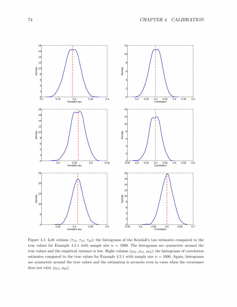
74 CHAPTER 4. CALIBRATION
0.1 0.15 0.2 0.25 0.30
2
4
6
8
10
12
14
16
18
Kendall’s tau
Den
sity
0.2 0.25 0.3 0.35 0.4 0.45 0.50
2
4
6
8
10
12
Correlation
Den
sity
0.2 0.25 0.3 0.350
2
4
6
8
10
12
14
16
18
Kendall’s tau
Den
sity
0.25 0.3 0.35 0.4 0.45 0.5 0.55 0.60
2
4
6
8
10
12
14
Correlation
Den
sity
0.35 0.4 0.45 0.50
5
10
15
20
25
Kendall’s tau
Den
sity
0.45 0.5 0.55 0.6 0.65 0.70
2
4
6
8
10
12
14
16
18
Correlation
Den
sity
Figure 4.1: Left column (τ12, τ13, τ23): the histograms of the Kendall’s tau estimates compared to thetrue values for Example 4.5.1 with sample size n = 1000. The histograms are symmetric around thetrue values and the empirical variance is low. Right column (ρ12, ρ13, ρ23): the histograms of correlationestimates compared to the true values for Example 4.5.1 with sample size n = 1000. Again, histogramsare symmetric around the true values and the estimation is accurate even in cases when the covariancedoes not exist (ρ13, ρ23).
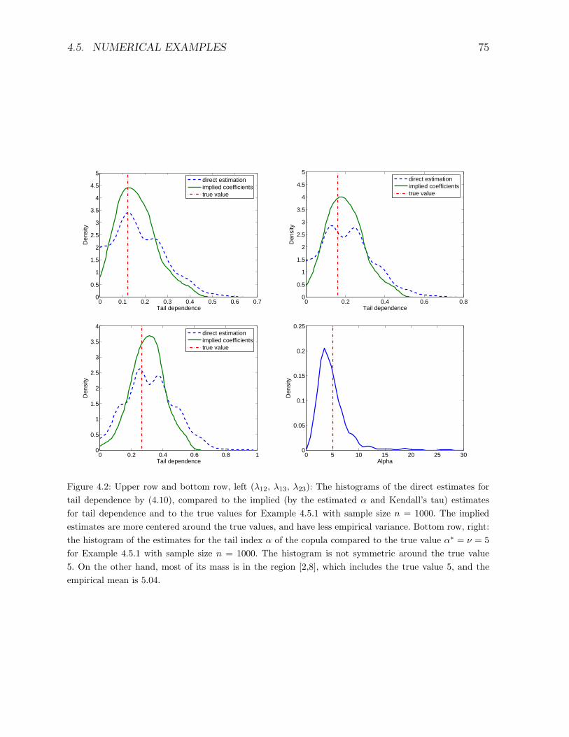
4.5. NUMERICAL EXAMPLES 75
0 0.1 0.2 0.3 0.4 0.5 0.6 0.70
0.5
1
1.5
2
2.5
3
3.5
4
4.5
5
Tail dependence
Den
sity
direct estimationimplied coefficientstrue value
0 0.2 0.4 0.6 0.80
0.5
1
1.5
2
2.5
3
3.5
4
4.5
5
Tail dependence
Den
sity
direct estimationimplied coefficientstrue value
0 0.2 0.4 0.6 0.8 10
0.5
1
1.5
2
2.5
3
3.5
4
Tail dependence
Den
sity
direct estimationimplied coefficientstrue value
0 5 10 15 20 25 300
0.05
0.1
0.15
0.2
0.25
Alpha
Den
sity
Figure 4.2: Upper row and bottom row, left (λ12, λ13, λ23): The histograms of the direct estimates fortail dependence by (4.10), compared to the implied (by the estimated α and Kendall’s tau) estimatesfor tail dependence and to the true values for Example 4.5.1 with sample size n = 1000. The impliedestimates are more centered around the true values, and have less empirical variance. Bottom row, right:the histogram of the estimates for the tail index α of the copula compared to the true value α∗ = ν = 5for Example 4.5.1 with sample size n = 1000. The histogram is not symmetric around the true value5. On the other hand, most of its mass is in the region [2,8], which includes the true value 5, and theempirical mean is 5.04.
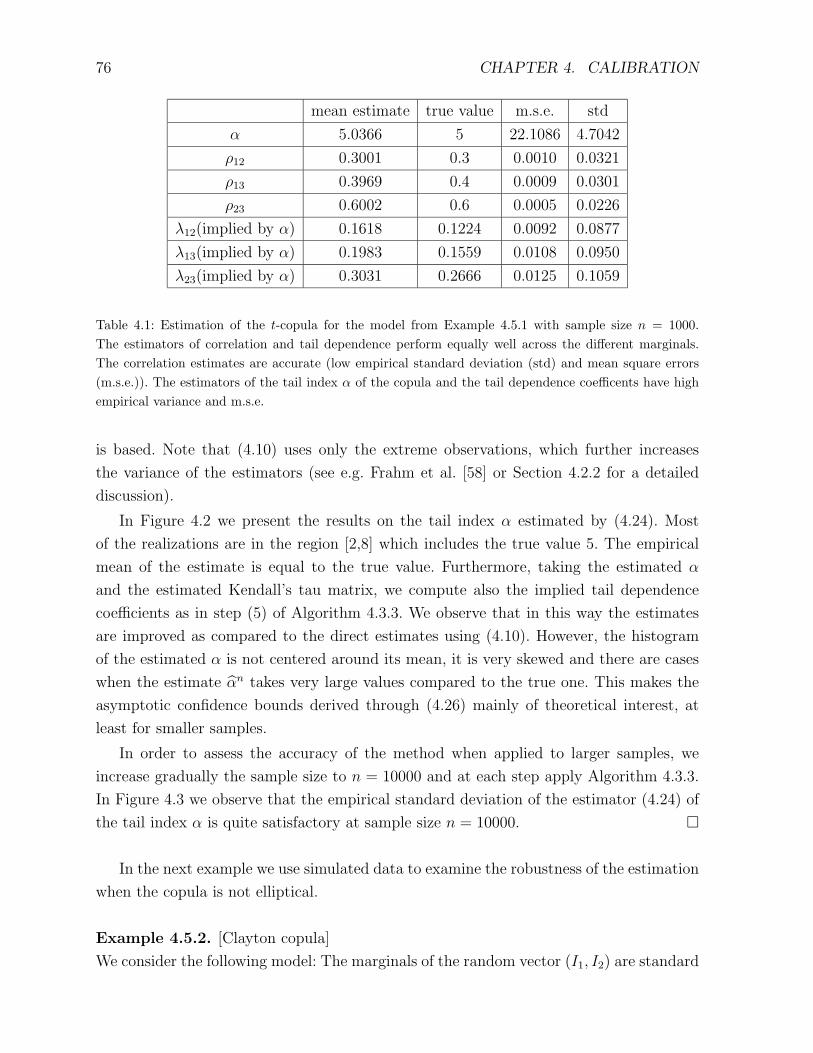
76 CHAPTER 4. CALIBRATION
mean estimate true value m.s.e. std
α 5.0366 5 22.1086 4.7042
ρ12 0.3001 0.3 0.0010 0.0321
ρ13 0.3969 0.4 0.0009 0.0301
ρ23 0.6002 0.6 0.0005 0.0226
λ12(implied by α) 0.1618 0.1224 0.0092 0.0877
λ13(implied by α) 0.1983 0.1559 0.0108 0.0950
λ23(implied by α) 0.3031 0.2666 0.0125 0.1059
Table 4.1: Estimation of the t-copula for the model from Example 4.5.1 with sample size n = 1000.The estimators of correlation and tail dependence perform equally well across the different marginals.The correlation estimates are accurate (low empirical standard deviation (std) and mean square errors(m.s.e.)). The estimators of the tail index α of the copula and the tail dependence coefficents have highempirical variance and m.s.e.
is based. Note that (4.10) uses only the extreme observations, which further increases
the variance of the estimators (see e.g. Frahm et al. [58] or Section 4.2.2 for a detailed
discussion).
In Figure 4.2 we present the results on the tail index α estimated by (4.24). Most
of the realizations are in the region [2,8] which includes the true value 5. The empirical
mean of the estimate is equal to the true value. Furthermore, taking the estimated α
and the estimated Kendall’s tau matrix, we compute also the implied tail dependence
coefficients as in step (5) of Algorithm 4.3.3. We observe that in this way the estimates
are improved as compared to the direct estimates using (4.10). However, the histogram
of the estimated α is not centered around its mean, it is very skewed and there are cases
when the estimate αn takes very large values compared to the true one. This makes the
asymptotic confidence bounds derived through (4.26) mainly of theoretical interest, at
least for smaller samples.
In order to assess the accuracy of the method when applied to larger samples, we
increase gradually the sample size to n = 10000 and at each step apply Algorithm 4.3.3.
In Figure 4.3 we observe that the empirical standard deviation of the estimator (4.24) of
the tail index α is quite satisfactory at sample size n = 10000.
In the next example we use simulated data to examine the robustness of the estimation
when the copula is not elliptical.
Example 4.5.2. [Clayton copula]
We consider the following model: The marginals of the random vector (I1, I2) are standard
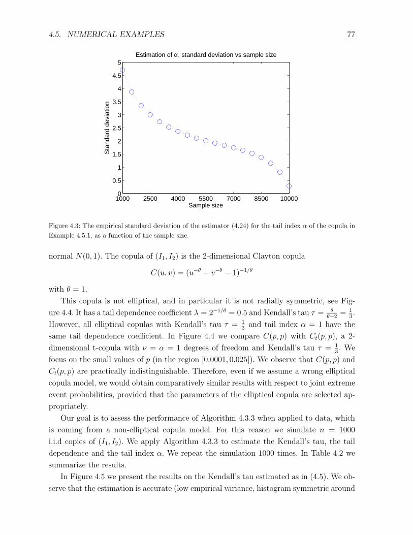
4.5. NUMERICAL EXAMPLES 77
1000 2500 4000 5500 7000 8500 100000
0.5
1
1.5
2
2.5
3
3.5
4
4.5
5
Sample size
Sta
ndar
d de
viat
ion
Estimation of α, standard deviation vs sample size
Figure 4.3: The empirical standard deviation of the estimator (4.24) for the tail index α of the copula inExample 4.5.1, as a function of the sample size.
normal N(0, 1). The copula of (I1, I2) is the 2-dimensional Clayton copula
C(u, v) = (u−θ + v−θ − 1)−1/θ
with θ = 1.
This copula is not elliptical, and in particular it is not radially symmetric, see Fig-
ure 4.4. It has a tail dependence coefficient λ = 2−1/θ = 0.5 and Kendall’s tau τ = θθ+2
= 13.
However, all elliptical copulas with Kendall’s tau τ = 13
and tail index α = 1 have the
same tail dependence coefficient. In Figure 4.4 we compare C(p, p) with Ct(p, p), a 2-
dimensional t-copula with ν = α = 1 degrees of freedom and Kendall’s tau τ = 13. We
focus on the small values of p (in the region [0.0001, 0.025]). We observe that C(p, p) and
Ct(p, p) are practically indistinguishable. Therefore, even if we assume a wrong elliptical
copula model, we would obtain comparatively similar results with respect to joint extreme
event probabilities, provided that the parameters of the elliptical copula are selected ap-
propriately.
Our goal is to assess the performance of Algorithm 4.3.3 when applied to data, which
is coming from a non-elliptical copula model. For this reason we simulate n = 1000
i.i.d copies of (I1, I2). We apply Algorithm 4.3.3 to estimate the Kendall’s tau, the tail
dependence and the tail index α. We repeat the simulation 1000 times. In Table 4.2 we
summarize the results.
In Figure 4.5 we present the results on the Kendall’s tau estimated as in (4.5). We ob-
serve that the estimation is accurate (low empirical variance, histogram symmetric around
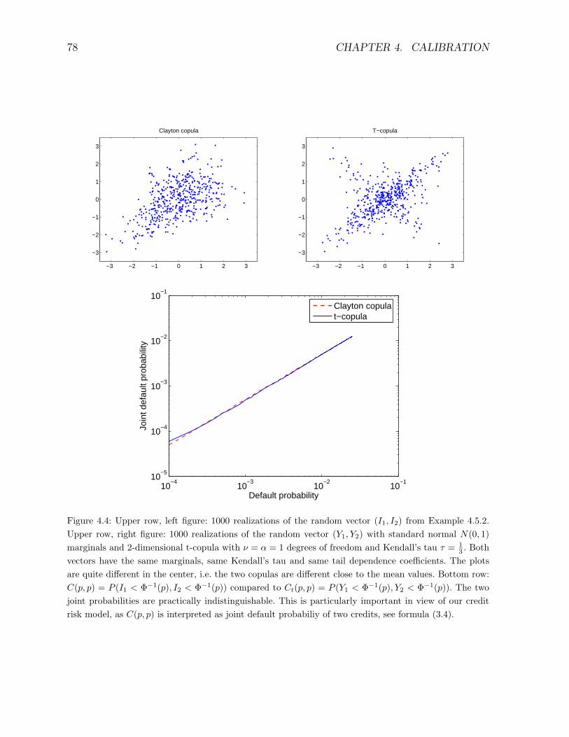
78 CHAPTER 4. CALIBRATION
−3 −2 −1 0 1 2 3
−3
−2
−1
0
1
2
3
Clayton copula
−3 −2 −1 0 1 2 3
−3
−2
−1
0
1
2
3
T−copula
10−4
10−3
10−2
10−1
10−5
10−4
10−3
10−2
10−1
Default probability
Join
t def
ault
prob
abili
ty
Clayton copulat−copula
Figure 4.4: Upper row, left figure: 1000 realizations of the random vector (I1, I2) from Example 4.5.2.Upper row, right figure: 1000 realizations of the random vector (Y1, Y2) with standard normal N(0, 1)marginals and 2-dimensional t-copula with ν = α = 1 degrees of freedom and Kendall’s tau τ = 1
3 . Bothvectors have the same marginals, same Kendall’s tau and same tail dependence coefficients. The plotsare quite different in the center, i.e. the two copulas are different close to the mean values. Bottom row:C(p, p) = P (I1 < Φ−1(p), I2 < Φ−1(p)) compared to Ct(p, p) = P (Y1 < Φ−1(p), Y2 < Φ−1(p)). The twojoint probabilities are practically indistinguishable. This is particularly important in view of our creditrisk model, as C(p, p) is interpreted as joint default probabiliy of two credits, see formula (3.4).
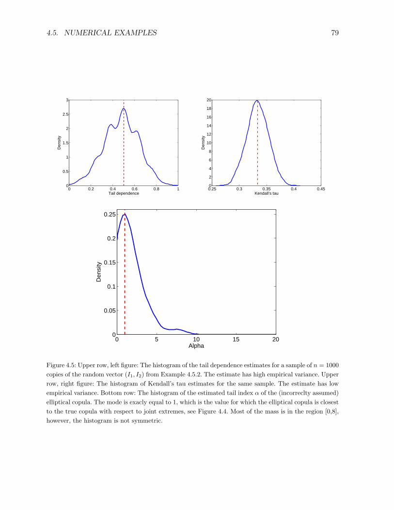
4.5. NUMERICAL EXAMPLES 79
0 0.2 0.4 0.6 0.8 10
0.5
1
1.5
2
2.5
3
Tail dependence
Den
sity
0.25 0.3 0.35 0.4 0.450
2
4
6
8
10
12
14
16
18
20
Kendall’s tau
Den
sity
0 5 10 15 200
0.05
0.1
0.15
0.2
0.25
Alpha
Den
sity
Figure 4.5: Upper row, left figure: The histogram of the tail dependence estimates for a sample of n = 1000copies of the random vector (I1, I2) from Example 4.5.2. The estimate has high empirical variance. Upperrow, right figure: The histogram of Kendall’s tau estimates for the same sample. The estimate has lowempirical variance. Bottom row: The histogram of the estimated tail index α of the (incorreclty assumed)elliptical copula. The mode is exacly equal to 1, which is the value for which the elliptical copula is closestto the true copula with respect to joint extremes, see Figure 4.4. Most of the mass is in the region [0,8],however, the histogram is not symmetric.
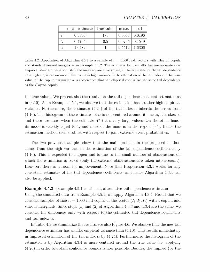
80 CHAPTER 4. CALIBRATION
mean estimate true value m.s.e. std
τ 0.3336 1/3 0.0003 0.0196
λ 0.4765 0.5 0.0235 0.1549
α 1.6482 1 9.5512 1.6306
Table 4.2: Application of Algorithm 4.3.3 to a sample of n = 1000 i.i.d. vectors with Clayton copulaand standard normal margins as in Example 4.5.2. The estimates for Kendall’s tau are accurate (lowempirical standard deviation (std) and mean square error (m.s.e)). The estimates for the tail dependencehave high empirical variance. This results in high variance in the estimation of the tail index α. The ’truevalue’ of the copula parameter α is chosen such that the elliptical copula has the same tail dependenceas the Clayton copula.
the true value). We present also the results on the tail dependence coeffient estimated as
in (4.10). As in Example 4.5.1, we observe that the estimation has a rather high empirical
variance. Furthermore, the estimator (4.24) of the tail index α inherits the errors from
(4.10). The histogram of the estimates of α is not centered around its mean, it is skewed
and there are cases when the estimate αn takes very large values. On the other hand,
its mode is exactly equal to 1, and most of the mass is in the region [0,5]. Hence the
estimation method seems robust with respect to joint extreme event probabilities.
The two previous examples show that the main problem in the proposed method
comes from the high variance in the estimation of the tail dependence coefficients by
(4.10). This is expected to happen and is due to the small number of observations on
which the estimation is based (only the extreme observations are taken into account).
However, there is a room for improvement. Note that Proposition 4.3.1 works for any
consistent estimates of the tail dependence coefficients, and hence Algorithm 4.3.4 can
also be applied.
Example 4.5.3. [Example 4.5.1 continued, alternative tail dependence estimator]
Using the simulated data from Example 4.5.1, we apply Algorithm 4.3.4. Recall that we
consider samples of size n = 1000 i.i.d copies of the vector (I1, I2, I3) with t-copula and
various marginals. Since steps (1) and (2) of Algorithms 4.3.3 and 4.3.4 are the same, we
consider the differences only with respect to the estimated tail dependence coefficients
and tail index α.
In Table 4.3 we summarize the results, see also Figure 4.6. We observe that the new tail
dependence estimator has smaller emprical variance than (4.10). This results immediately
in improved estimation of the tail index α by (4.24). Furthermore, the histogram of the
estimated α by Algorithm 4.3.4 is more centered around the true value, i.e. applying
(4.26) in order to obtain confidence bounds is now possible. Besides, the implied (by the
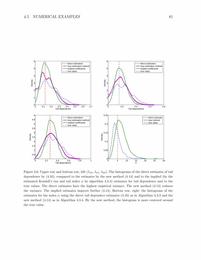
4.5. NUMERICAL EXAMPLES 81
0 0.1 0.2 0.3 0.4 0.5 0.6 0.70
1
2
3
4
5
6
Tail dependence
Den
sity
direct estimationnew estimation methodimplied coefficientstrue value
0 0.2 0.4 0.6 0.80
1
2
3
4
5
6
Tail dependence
Den
sity
direct estimationnew estimation methodimplied coefficientstrue value
0 0.2 0.4 0.6 0.8 10
0.5
1
1.5
2
2.5
3
3.5
4
4.5
5
Tail dependence
Den
sity
direct estimationnew estimation methodimplied coefficientstrue value
0 5 10 15 20 25 300
0.05
0.1
0.15
0.2
0.25
α
Den
sity
direct estimatenew methodtrue value
Figure 4.6: Upper row and bottom row, left (λ12, λ13, λ23): The histograms of the direct estimates of taildependence by (4.10), compared to the estimates by the new method (4.14) and to the implied (by theestimated Kendall’s tau and tail index α by algorithm 4.3.4) estimates for tail dependence and to thetrue values. The direct estimates have the highest empirical variance. The new method (4.14) reducesthe variance. The implied estimates improve further (4.14). Bottom row, right: the histograms of theestimates for the index α using the direct tail dependece estimates (4.10) as in Algorithm 4.3.3 and thenew method (4.14) as in Algorithm 4.3.4. By the new method, the histogram is more centered aroundthe true value.
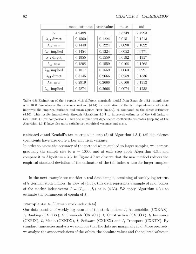
82 CHAPTER 4. CALIBRATION
mean estimate true value m.s.e std
α 4.9488 5 5.8749 2.4293
λ12 direct
λ12 new
λ12 implied
0.1560
0.1440
0.1454
0.1224
0.1224
0.1224
0.0151
0.0090
0.0052
0.1213
0.1022
0.0771
λ13 direct
λ13 new
λ13 implied
0.1955
0.1808
0.1817
0.1559
0.1559
0.1559
0.0192
0.0108
0.0063
0.1357
0.1268
0.0991
λ23 direct
λ23 new
λ23 implied
0.3145
0.2919
0.2874
0.2666
0.2666
0.2666
0.0259
0.0166
0.0074
0.1536
0.1352
0.1238
Table 4.3: Estimation of the t-copula with different marginals model from Example 4.5.1, sample sizen = 1000. We observe that the new method (4.14) for estimation of the tail dependence coefficientsimproves the empirical variance and mean square error (m.s.e.), as compared to the direct estimator(4.10). This results immediately through Algorithm 4.3.4 in improved estimates of the tail index α
(see Table 4.1 for comparison). Then the implied tail dependence coefficients estimates (step (5) of theAlgorithm 4.3.4) have also quite satisfactory empirical variance and m.s.e.
estimated α and Kendall’s tau matrix as in step (5) of Algorithm 4.3.4) tail dependence
coefficients have also quite a low empirical variance.
In order to assess the accuracy of the method when applied to larger samples, we increase
gradually the sample size to n = 10000 and at each step apply Algorithm 4.3.4 and
compare it to Algorithm 4.3.3. In Figure 4.7 we observe that the new method reduces the
empirical standard deviation of the estimator of the tail index α also for larger samples.
In the next example we consider a real data sample, consisting of weekly log-returns
of 8 German stock indices. In view of (4.33), this data represents a sample of i.i.d. copies
of the market index vector I = (I1, . . . , I8) as in (4.33). We apply Algorithm 4.3.4 to
estimate the parameters of copula of I.
Example 4.5.4. [German stock index data]
Our data consists of weekly log-returns of the stock indices: I1 Automobiles (CXKAX),
I2 Banking (CXKBX), I3 Chemicals (CXKCX), I4 Construction (CXKOX), I5 Insurance
(CXPIX), I6 Media (CXKDX), I7 Software (CXKSX) and I8 Transport (CXKTX). By
standard time series analysis we conclude that the data are marginally i.i.d. More precisely,
we analyse the autocorrelations of the values, the absolute values and the squared values in
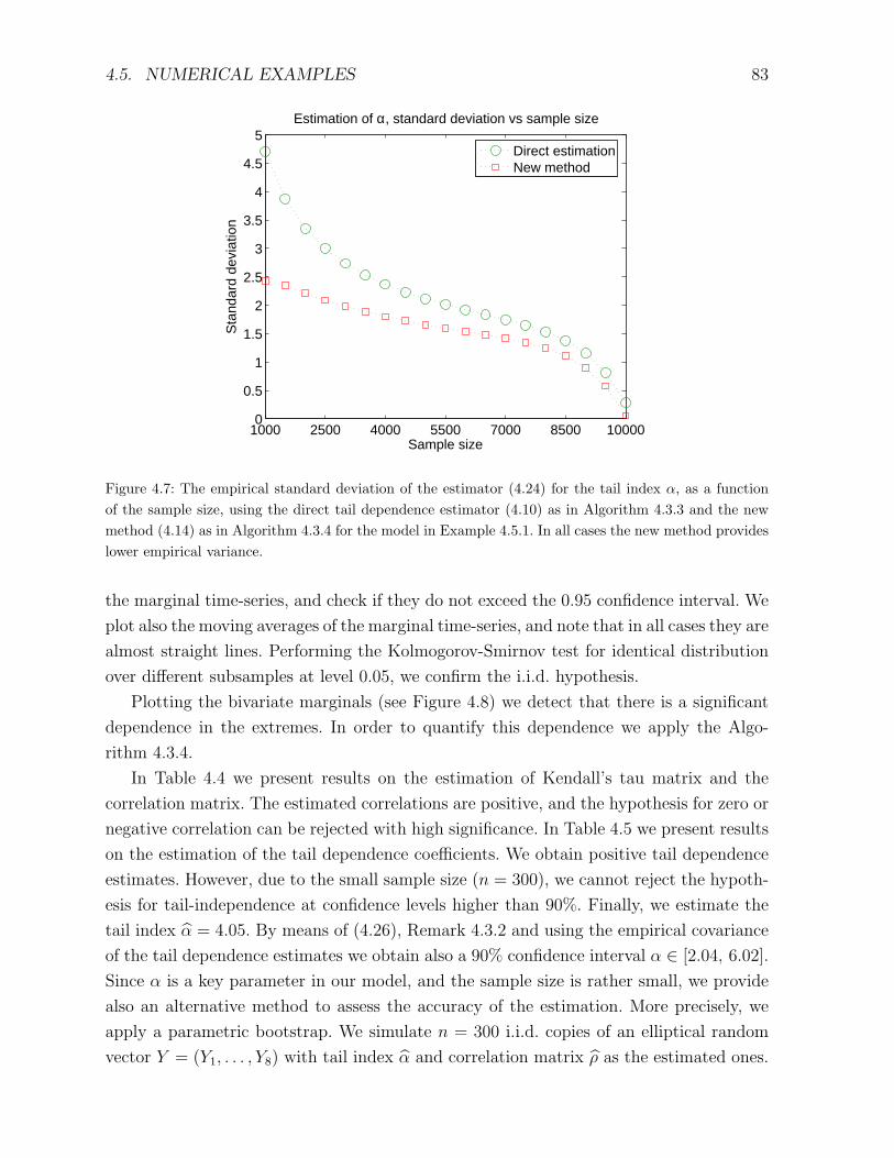
4.5. NUMERICAL EXAMPLES 83
1000 2500 4000 5500 7000 8500 100000
0.5
1
1.5
2
2.5
3
3.5
4
4.5
5Estimation of α, standard deviation vs sample size
Sample size
Sta
ndar
d de
viat
ion
Direct estimationNew method
Figure 4.7: The empirical standard deviation of the estimator (4.24) for the tail index α, as a functionof the sample size, using the direct tail dependence estimator (4.10) as in Algorithm 4.3.3 and the newmethod (4.14) as in Algorithm 4.3.4 for the model in Example 4.5.1. In all cases the new method provideslower empirical variance.
the marginal time-series, and check if they do not exceed the 0.95 confidence interval. We
plot also the moving averages of the marginal time-series, and note that in all cases they are
almost straight lines. Performing the Kolmogorov-Smirnov test for identical distribution
over different subsamples at level 0.05, we confirm the i.i.d. hypothesis.
Plotting the bivariate marginals (see Figure 4.8) we detect that there is a significant
dependence in the extremes. In order to quantify this dependence we apply the Algo-
rithm 4.3.4.
In Table 4.4 we present results on the estimation of Kendall’s tau matrix and the
correlation matrix. The estimated correlations are positive, and the hypothesis for zero or
negative correlation can be rejected with high significance. In Table 4.5 we present results
on the estimation of the tail dependence coefficients. We obtain positive tail dependence
estimates. However, due to the small sample size (n = 300), we cannot reject the hypoth-
esis for tail-independence at confidence levels higher than 90%. Finally, we estimate the
tail index α = 4.05. By means of (4.26), Remark 4.3.2 and using the empirical covariance
of the tail dependence estimates we obtain also a 90% confidence interval α ∈ [2.04, 6.02].
Since α is a key parameter in our model, and the sample size is rather small, we provide
also an alternative method to assess the accuracy of the estimation. More precisely, we
apply a parametric bootstrap. We simulate n = 300 i.i.d. copies of an elliptical random
vector Y = (Y1, . . . , Y8) with tail index α and correlation matrix ρ as the estimated ones.

84 CHAPTER 4. CALIBRATION
CXKAX CXKBX CXKCX CXKOX CXPIX CXKDX CXKSX CXKTX
I1
τij
90%CI
ρij
90%CI
0.47
[.39 .55]
0.67
[.57 .76]
0.44
[.34 .54]
0.64
[.51 .75]
0.26
[.11 .41]
0.40
[.18 .60]
0.36
[.24 .48]
0.54
[.37 .69]
0.18
[.04 .32]
0.28
[.06 .49]
0.34
[.22 .48]
0.52
[.34 .68]
0.44
[.34 .55]
0.64
[.50 .76]
I2
0.47
[.39 .55]
0.67
[.57 .76]
τij
90%CI
ρij
90%CI
0.46
[.36 .56]
0.66
[.53 .77]
0.27
[.11 .44]
0.42
[.17 .63]
0.51
[.41 .60]
0.72
[.60 .81]
0.23
[.10 .36]
0.35
[.15 .54]
0.38
[.26 .50]
0.56
[.39 .71]
0.48
[.39 .57]
0.68
[.57 .78]
I3
0.44
[.34 .54]
0.64
[.51 .75]
0.46
[.36 .56]
0.66
[.53 .77]
τij
90%CI
ρij
90%CI
0.24
[.08 .40]
0.37
[.13 .59]
0.43
[.32 .53]
0.62
[.49 .74]
0.17
[.03 .32]
0.27
[.05 .48]
0.28
[.12 .43]
0.42
[.19 .62]
0.47
[.38 .57]
0.69
[.56 .78]
I4
0.26
[.11 .41]
0.40
[.18 .60]
0.27
[.11 .44]
0.42
[.17 .63]
0.24
[.08 .40]
0.37
[.13 .59]
τij
90%CI
ρij
90%CI
0.28
[.13 .43]
0.43
[.20 .63]
0.17
[.02 .32]
0.27
[.03 .49]
0.17
[.00 .34]
0.26
[.00 .50]
0.30
[.14 .46]
0.46
[.22 .66]
I5
0.36
[.24 .48]
0.54
[.37 .69]
0.51
[.41 .60]
0.72
[.60 .81]
0.43
[.32 .53]
0.62
[.49 .74]
0.28
[.13 .43]
0.43
[.20 .63]
τij
90%CI
ρij
90%CI
0.21
[.08 .34]
0.33
[.13 .51]
0.35
[.22 .48]
0.52
[.34 .68]
0.42
[.29 .54]
0.61
[.45 .75]
I6
0.18
[.04 .32]
0.28
[.06 .49]
0.23
[.10 .36]
0.35
[.15 .54]
0.17
[.03 .32]
0.27
[.05 .48]
0.17
[.02 .32]
0.27
[.03 .49]
0.21
[.08 .34]
0.33
[.13 .51]
τij
90%CI
ρij
90%CI
0.31
[.17 .44]
0.46
[.27 .64]
0.27
[.15 .40]
0.42
[.23 .59]
I7
0.34
[.22 .48]
0.52
[.34 .68]
0.38
[.26 .50]
0.56
[.39 .71]
0.28
[.12 .43]
0.42
[.19 .62]
0.17
[.00 .34]
0.26
[.00 .50]
0.35
[.22 .48]
0.52
[.34 .68]
0.31
[.17 .44]
0.46
[.27 .64]
τij
90%CI
ρij
90%CI
0.40
[.28 0.53]
0.59
[.42 .74]
I8
0.44
[.34 .55]
0.64
[.50 .76]
0.48
[.39 .57]
0.68
[.57 .78]
0.47
[.38 .57]
0.69
[.56 .78]
0.30
[.14 .46]
0.46
[.22 .66]
0.42
[.29 .54]
0.61
[.45 .75]
0.27
[.15 .40]
0.42
[.23 .59]
0.40
[.28 .53]
0.59
[.42 .74]
τij
90%CI
ρij
90%CI
Table 4.4: Estimation of Kendall’s tau and correlation for the German stock index data from Example 4.5.4. In brackets are given the 90% confidence intervals, based on the empirical variance.

4.5. NUMERICAL EXAMPLES 85
CXKAX CXKBX CXKCX CXKOX CXPIX CXKDX CXKSX CXKTX
I1
λij
90%UB
λIij
.28
.64
.36
.16
.36
.34
.16
.35
.20
.13
.29
.27
.25
.57
.15
.27
.60
.26
.25
.56
.34
I2
.28
.64
.36
λij
90%UB
λIij
.16
.36
.35
.46
.99
.20
.42
.95
.40
.16
.36
.18
.16
.36
.28
.40
.90
.37
I3
.16
.36
.34
.16
.36
.35
λij
90%UB
λIij
.16
.36
.19
.13
.29
.32
.16
.36
.15
.25
.58
.20
.25
.58
.37
I4
.16
.35
.20
.46
.99
.20
.16
.36
.19
λij
90%UB
λIij
.32
.72
.21
.16
.35
.15
.16
.37
.15
.43
.98
.23
I5
.13
.29
.27
.42
.95
.40
.13
.29
.32
.32
.72
.21
λij
90%UB
λIij
.12
.29
.17
.21
.48
.26
.57
.99
.31
I6
.25
.57
.15
.16
.36
.18
.16
.36
.15
.16
.35
.15
.12
.29
.17
λij
90%UB
λIij
.31
.71
.23
.31
.72
.20
I7
.27
.60
.26
.16
.36
.28
.25
.58
.20
.16
.37
.15
.21
.48
.26
.31
.71
.23
λij
90%UB
λIij
.47
.99
.30
I8
.25
.56
.34
.40
.90
.37
.25
.58
.37
.43
.98
.23
.57
.99
.31
.31
.72
.20
.47
.99
.30
λij
90%UB
λIij
Table 4.5: Estimated tail dependence matrix and implied tail dependence matrix (step (5) of Algo-rithm 4.3.4) for the German stock indices from Example 4.5.4. In the second rows are given the 90%upper confidence bounds, based on the empirical variance.
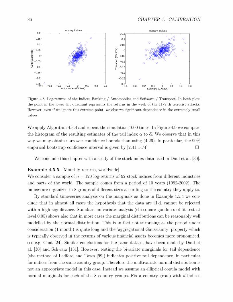
86 CHAPTER 4. CALIBRATION
−0.4 −0.3 −0.2 −0.1 0 0.1 0.2 0.3−0.25
−0.2
−0.15
−0.1
−0.05
0
0.05
0.1
0.15
0.2
Automobiles (CXKAX)
Ban
king
(C
XK
BX
)Industry Indices
−0.4 −0.3 −0.2 −0.1 0 0.1 0.2 0.3−0.3
−0.25
−0.2
−0.15
−0.1
−0.05
0
0.05
0.1
0.15Industry Indices
Software (CXKSX)
Tra
nspo
rt (
CX
KT
X)
Figure 4.8: Log-returns of the indices Banking / Automobiles and Software / Transport. In both plotsthe point in the lower left quadrant represents the returns in the week of the 11/9’th terrorist attacks.However, even if we ignore this extreme point, we observe significant dependence in the extremely smallvalues.
We apply Algorithm 4.3.4 and repeat the simulation 1000 times. In Figure 4.9 we compare
the histogram of the resulting estimates of the tail index α to α. We observe that in this
way we may obtain narrower confidence bounds than using (4.26). In particular, the 90%
empirical bootstrap confidence interval is given by [2.41, 5.74]
We conclude this chapter with a study of the stock index data used in Daul et al. [30].
Example 4.5.5. [Monthly returns, worldwide]
We consider a sample of n = 120 log-returns of 92 stock indices from different industries
and parts of the world. The sample comes from a period of 10 years (1992-2002). The
indices are organized in 8 groups of different sizes according to the country they apply to.
By standard time-series analysis on the marginals as done in Example 4.5.4 we con-
clude that in almost all cases the hypothesis that the data are i.i.d. cannot be rejected
with a high significance. Standard univariate analysis (chi-square goodness-of-fit test at
level 0.05) shows also that in most cases the marginal distributions can be reasonably well
modelled by the normal distribution. This is in fact not surprising as the period under
consideration (1 month) is quite long and the ’aggregational Gaussianity’ property which
is typically observed in the returns of various financial assets becomes more pronounced,
see e.g. Cont [24]. Similar conclusions for the same dataset have been made by Daul et
al. [30] and Schwarz [131]. However, testing the bivariate marginals for tail dependence
(the method of Ledford and Tawn [99]) indicates positive tail dependence, in particular
for indices from the same country group. Therefore the multivariate normal distribution is
not an appropriate model in this case. Instead we assume an elliptical copula model with
normal marginals for each of the 8 country groups. Fix a country group with d indices
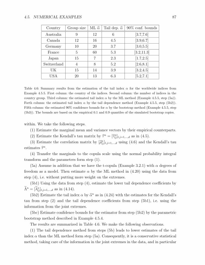
4.5. NUMERICAL EXAMPLES 87
Country Group size ML α Tail dep. α 90% conf. bounds
Australia 9 12 6 [3.7,7.6]
Canada 12 16 4.5 [3.9,6.7]
Germany 10 20 3.7 [3.0,5.5]
France 5 60 5.3 [3.2,11.3]
Japan 15 7 2.3 [1.7,2.5]
Switzerland 4 8 5.2 [2.6,8.1]
UK 15 14 3.9 [3.2,4.5]
USA 20 13 6.3 [5.2,7.1]
Table 4.6: Summary results from the estimation of the tail index α for the worldwide indices fromExample 4.5.5. First column: the country of the indices. Second column: the number of indices in thecountry group. Third column: the estimated tail index α by the ML method (Example 4.5.5, step (5a)).Forth column: the estimated tail index α by the tail dependence method (Example 4.5.5, step (5b2)).Fifth column: the estimated 90% confidence bounds for α by the bootstrap method (Example 4.5.5, step(5b3)). The bounds are based on the empirical 0.1 and 0.9 quantiles of the simulated bootstrap copies.
within. We take the following steps.
(1) Estimate the marginal mean and variance vectors by their empirical counterparts.
(2) Estimate the Kendall’s tau matrix by τn = [τnlj]l,j=1,...,d as in (4.5).
(3) Estimate the correlation matrix by [ρnlj]l,j=1,...,d using (4.6) and the Kendall’s tau
estimates τn.
(4) Transfer the marginals to the copula scale using the normal probability integral
transform and the parameters form step (1).
(5a) Assume in addition that we have the t-copula (Example 3.2.1) with α degrees of
freedom as a model. Then estimate α by the ML method in (4.20) using the data from
step (4), i.e. without putting more weight on the extremes.
(5b1) Using the data from step (4), estimate the lower tail dependence coefficients by
Λn = [λnlj]l,j=1,...,d as in (4.14).
(5b2) Estimate the tail index α by αn as in (4.24) with the estimates for the Kendall’s
tau from step (2) and the tail dependence coefficients from step (5b1), i.e. using the
information from the joint extremes.
(5bc) Estimate confidence bounds for the estimator from step (5b2) by the parametric
bootstrap method described in Example 4.5.4.
The results are summarized in Table 4.6. We make the following observations.
(1) The tail dependence method from steps (5b) leads to lower estimates of the tail
index α than the ML method form step (5a). Consequently, it is a conservative statistical
method, taking care of the information in the joint extremes in the data, and in particular
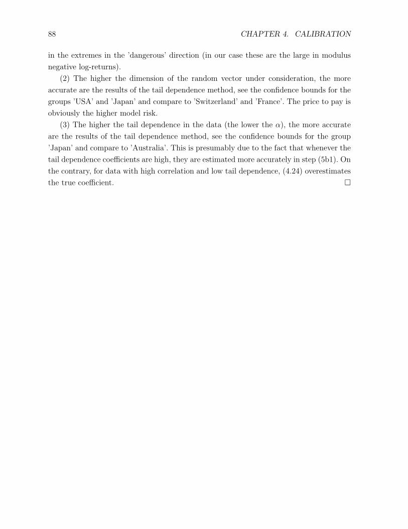
88 CHAPTER 4. CALIBRATION
in the extremes in the ’dangerous’ direction (in our case these are the large in modulus
negative log-returns).
(2) The higher the dimension of the random vector under consideration, the more
accurate are the results of the tail dependence method, see the confidence bounds for the
groups ’USA’ and ’Japan’ and compare to ’Switzerland’ and ’France’. The price to pay is
obviously the higher model risk.
(3) The higher the tail dependence in the data (the lower the α), the more accurate
are the results of the tail dependence method, see the confidence bounds for the group
’Japan’ and compare to ’Australia’. This is presumably due to the fact that whenever the
tail dependence coefficients are high, they are estimated more accurately in step (5b1). On
the contrary, for data with high correlation and low tail dependence, (4.24) overestimates
the true coefficient.
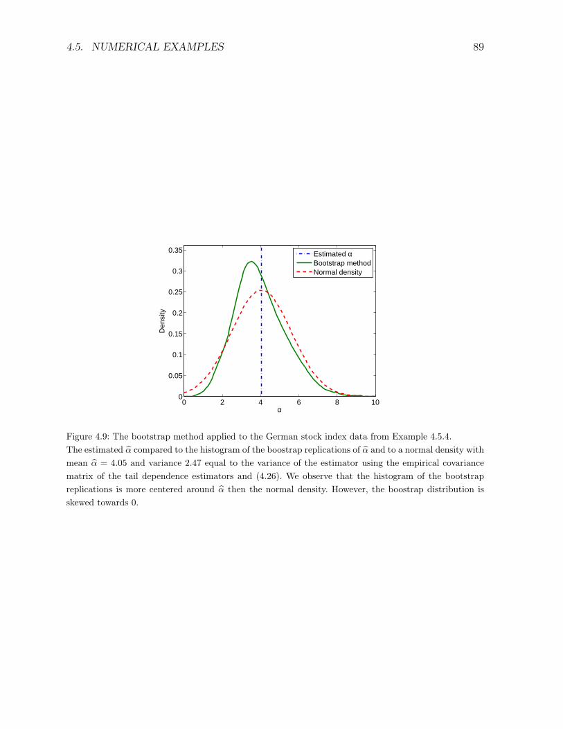
4.5. NUMERICAL EXAMPLES 89
0 2 4 6 8 100
0.05
0.1
0.15
0.2
0.25
0.3
0.35
α
Den
sity
Estimated αBootstrap methodNormal density
Figure 4.9: The bootstrap method applied to the German stock index data from Example 4.5.4.The estimated α compared to the histogram of the boostrap replications of α and to a normal density withmean α = 4.05 and variance 2.47 equal to the variance of the estimator using the empirical covariancematrix of the tail dependence estimators and (4.26). We observe that the histogram of the bootstrapreplications is more centered around α then the normal density. However, the boostrap distribution isskewed towards 0.

90 CHAPTER 4. CALIBRATION
Chapter 5
Simulation
In this chapter we begin the analysis of the portfolio loss distribution in model (3.1) with
(3.4) and (3.5). In Section 5.1 we present an algorithm for straightforward simulation of
the loss L. As its application to practical problems is computationally intensive, in Sec-
tion 5.2.2 we provide an improved algorithm, using a classical variance reduction technique
– importance sampling. We pay particular attention to its application in the framework
of heavy-tailed risk factors. Numerical support for our method is given in Section 5.3.1.
Using Monte Carlo simulation, we illustrate the impact of the heavy-tailed model for the
risk factors on the tail of the portfolio loss distribution in Section 5.3.2.
5.1 Direct Monte Carlo simulation
Monte Carlo simulation is among the most widely used computational tools in risk man-
agement. As in other application areas, it has the advantage of being very general and
the disadvantage of being rather slow. In model (3.1) with (3.4) and (3.5) this procedure
has essentially three steps.
Algorithm 5.1.1. Monte Carlo simulation of L.
(1) Simulate the asset returns Y = (Y1, . . . , Ym).
(2) Determine the ratings X = (X1, . . . , Xm) by means of (3.4).
(3) Given X = (X1, . . . , Xm), simulate (L1, . . . , Lm) and compute L =∑m
j=1 ejLj.
Simulation of Y = (Y1, . . . , Ym) is relatively easy, as this vector has a NVM distribu-
tion. We apply the following algorithm as in Embrechts et al. [47].
Algorithm 5.1.2. Monte Carlo simulation of a NVM distribution.
(1) Find the Choleski decomposition A of the covariance matrix ΣY (i.e. AA′ = ΣY ).
(2) Simulate m independent standard normals Z = (Z1, . . . , Zm).
91
92 CHAPTER 5. SIMULATION
(3) Simulate an independent W .
(4) Compute Y = WBZ.
However, several features of the credit risk setting pose a particular challenge to this
approach.
(1) It requires accurate estimation of low-probability events, e.g. the probability of an
extremely high loss. Hence, only a small part of the simulated data is used.
(2) Portfolios are multidimensional, i.e. m is large, and a large quantity of random
numbers has to be drawn.
(3) Straightforward simulation of heavy-tailed r.v.s like Y1, . . . , Ym produces notori-
ously poor results, see Glasserman [69].
Therefore alternative approaches are needed.
5.2 Importance sampling (IS)
5.2.1 General IS algorithms
Importance sampling is a classical variance reduction technique. Consider for a moment
a general problem for estimating c = P (F (Y ) ≥ x) = E[1F (Y )>x
]for some random
vector Y with density g and range D ⊆ Rp and some function F . The most simple way is
to sample independent Y (1), Y (2), . . . , Y (N) and take the average
cMC =1
N
N∑i=1
1F (Y (i))≥x
as an estimate. However,
E[1F (Y )≥x
]=
∫D
1F (Y )≥xg(y)dy
=
∫D
1F (Y )≥xg(y)f(y)
f(y)dy
= E
[1F (Y )≥x
g(Y )
f(Y )
],
where f is another density with the property g(y) > 0 ⇒ f(y) > 0, y ∈ D, and Y is a
r.v. with density f . Then
cIS =1
N
N∑i=1
1F (Y (i))≥xg(Y (i))
f(Y (i)),
where Y (1), Y (2), . . . Y (N) are i.i.d copies of Y is again an estimator for c. The quantity
g/f is called likelihood ratio.
5.2. IMPORTANCE SAMPLING (IS) 93
The goal in an importance sampling procedure is to select the density f such that
the variance (or equivalently the second moment) of the estimator cIS is minimized. As
shown for instance in Glasserman et al. [68], deriving the optimal (zero variance) density
is equivalent to knowing the desired quantity c. Hence, some approximation of the optimal
density is needed.
A classical method for selection of the density f is exponential twisting. Suppose
that the components of Y = (Y1, . . . , Yp) are independent with densities g1, . . . , gp, hence
g (y) =
p∏l=1
gl (y) , y ∈ D .
Then we select fl, l = 1, . . . , p, from the parametric family
fl (y) =exp(µly)
E [exp(µlYl)]gl(y) , y ∈ D ,
for some µ = (µ1, . . . , µp), provided that E [exp(µlYl)] exists. The likelihood ratio becomes
g (y)
f (y)=
p∏l=1
E [exp(µlYl)]
exp(µly), y ∈ D .
The optimal µ = (µ1, . . . , µp) minimizes the second moment of cIS, i.e.
µ = arg minµE
1F (Y )>x
(p∏l=1
E [exp(µlYl)]
exp(µlYl)
)2 = arg min
µE[c2IS
], (5.1)
where Y = (Y1, . . . , Yp) has a density f(y) =∏p
l=1 fl(yl) Unfortunately, in most cases
this problem is also infeasible (see Glasserman et al. [68]), and a further approximation is
necessary. The typically used approximation is based on the classical Laplace method for
integrals, see e.g. Dupois and Ellis [43], Chapter 3. Given that the function F is increasing
componentwisely, one may replace (5.1) by
µ = arg minµ
(p∏l=1
E [exp(µlYl)]
exp(µlyl(µl))
), (5.2)
where
y(µ) = (y1(µ)), . . . , yp(µ)) = arg maxy:F (y)=x
p∑l=1
µlyl ,
see e.g. Glasserman et al. [68] for a detailed reasoning behind this method.
94 CHAPTER 5. SIMULATION
5.2.2 IS for portfolio credit risk
To motivate the approach we take in the credit risk model (3.1) with (3.4) and (3.5),
observe that for every estimator c of P (L > x) and for every random vector ξ on the same
probability space we have the variance decomposition
var[c] = E[var[c | ξ]] + var[E[c | ξ]] . (5.3)
We try to minimize the two parts of (5.3) separately. To do this we need a proper
random vector ξ. Bearing in mind that, given the global shock W and the common
factors Z, the individual credits in the portfolio are independent (see Section 3.3), we
select ξ = (W,Z).
First we try to minimize the conditional (on W,Z) variance of the estimator. i.e.
the first term in (5.3). Let θ > 0 be a fixed constant. Let Xθ =(Xθ
1 , . . . , Xθm
)be a
random vector with discrete marginals with range 1, 2, . . . , K defined on the conditional
probability space (Ω,F , PW,Z = P (·|W,Z)). Let also Xθ1 , . . . , X
θm be independent with
PW,Z(Xθj = s
)=
gj,s(W,Z)ϕj,s(ejθ)∑Kk=1 gj,k(W,Z)ϕj,k(ejθ)
= qj,s(W,Z) , j = 1, . . . ,m , s = 1, . . . , K
(5.4)
where gj,k and ϕj,k are defined as in (3.11) and (3.12) respectively.
Consider the r.v.
Lθ =m∑j=1
ejLθj (5.5)
where for j = 1, . . . ,m:
- ej is the known positive constant from (3.1);
- Lθj is a real-valued r.v., defined on the conditional probability space(Ω,F , P (·|Xθ
j ))
and its density is given by
dP(Lθj < x |Xθ
j
)=
exp(ejθx)
ϕj,Xj(ejθ)dP(Lj < x |Xj = Xθ
j
), (5.6)
where Lj is defined as in (3.1).
Under these assumptions, we have:
(A1) From Assumption (A) in (3.1), we have that Lθj are conditionally independent,
given Xθ.
(B1) From Assumption (B) in (3.1), we have that given Xθj , Lθj is independent of Xθ
s
for s = 1, . . . ,m, s 6= j.
(C1) From Assumption (C) in (3.1), we have that Cj ≤ Lθj ≤ 1 a.s.
5.2. IMPORTANCE SAMPLING (IS) 95
Lemma 5.2.1. Under the assumptions of model (3.1) with (3.4) and (3.5), the density
of the r.v. Lθ defined in (5.5) is given by:
dPW,Z(Lθ < x
)=
exp(θx)
exp(H(W,Z, θ))dPW,Z (L < x) ,
where H(W,Z, θ) is defined in (3.8).
Proof. Denote E[·] = E[· |W,Z] and ϕ(τ) = E[exp(τLθ)]. We have
ϕ(τ) = E[E[exp(τLθ) |Xθ]]
= E[m∏j=1
E[exp(τejLθj) |Xθ
j ]]
because of (A1) and (B1). By (5.4) we get
ϕ(τ) = E[m∏j=1
K∑s=1
qj,s(W,Z)E[exp(τejLθj) |Xθ
j = s]]
= E[m∏j=1
K∑s=1
qj,s(W,Z)E[exp((τ + θ)ejLj) |Xj = s]
ϕj,s(ejθ)]
due to (5.6). Therefore
ϕ(τ) = E[m∏j=1
K∑s=1
gj,s(W,Z)ϕj,s(ejθ)∑Kk=1 gj,k(W,Z)ϕj,k(ejθ)
ϕj,s(ej(θ + τ))
ϕj,s(ejθ)]
= E[m∏j=1
∑Ks=1 gj,s(W,Z)ϕj,s(ej(θ + τ))∑K
k=1 gj,k(W,Z)ϕj,k(ejθ)]
=exp(H(W,Z, θ + τ))
exp(H(W,Z, θ))
by the definition of H in (3.8). Therefore
E[exp(τLθ)] =
∫R
exp(τx)dPW,Z(Lθ < x)
=
∫R
exp(τx)exp(θx)dPW,Z(L < x)
exp(H(W,Z, θ))
which proves the lemma.
By means of the above lemma,
P (L > x |W,Z) = E[1L>x] = E[1Lθ>x exp(H(W,Z, θ)− θLθ)] .
This result suggests the following simulation algorithm for estimation of P (L > x):
96 CHAPTER 5. SIMULATION
Algorithm 5.2.2. (1) Simulate the global shock W and the common factors Z =
(Z1, . . . , Zp).
(2a) If E[L |W,Z] ≥ x, then the event L > x is not rare. In this case we draw
(X01 , . . . , X
0m) = (X1, . . . , Xm) as in (5.4). Then we draw (L0
1, . . . , L0m) = (L1, . . . , Lm) as
in (5.6), compute L0 = L as (5.5) and return
1L0>x = 1L>x
as an estimator for P (L > x).
(2b) If E[L |W,Z] < x, we select some θ = θ(W,Z) > 0 and we draw (Xθ1 , . . . , X
θm) as
in (5.4). Then we draw (Lθ1, . . . , Lθm) as in (5.6), compute Lθ as (5.5) and return
1Lθ>x exp(H(W,Z, θ)− θLθ)]
as an estimator for P (L > x).
(3) Average over N independent random draws.
Step (1) of the above algorithm is trivial, as it requires a simulation of a one-dimensional
r.v. W and the multivariate normal Z. We compute immediately
E[L] =m∑j=1
ejgj,k(W,Z)(Xj = k)µj,k ,
where µj,k are as in Proposition 3.3.2 and gj,k are given in (3.11), j = 1, . . . ,m, k =
1, . . . , K. Therefore we can directly determine whether we are in regime (2a) or (2b).
Step (2a) is also straightforward. The hardest point in step (2b) is the selection of an
appropriate θ = θ(W,Z). Theoretically, we have to minimize the second moment of the
estimator (in other words, the first summand in (5.3)), i.e. to choose
θ = arg minθE[1Lθ>x exp(2H(W,Z, θ)− 2θLθ)] .
As this problem is infeasible, we use the bound
E[1Lθ>x exp(2H(W,Z, θ)− 2θLθ)] ≤ exp(2H(W,Z, θ)− 2θx) .
Instead of minimizing the integral, we minimize its upper bound and get
θ = arg minθH(W,Z, θ)− θx .
Various considerations lead to such a choice, see Glasserman [68] or Glasserman and Li [70]
for a detailed discussion. In particular, with this choice we obtain from Lemma 5.2.1 that
E[Lθ] = x, which makes the event Lθ > x common, rather than rare.
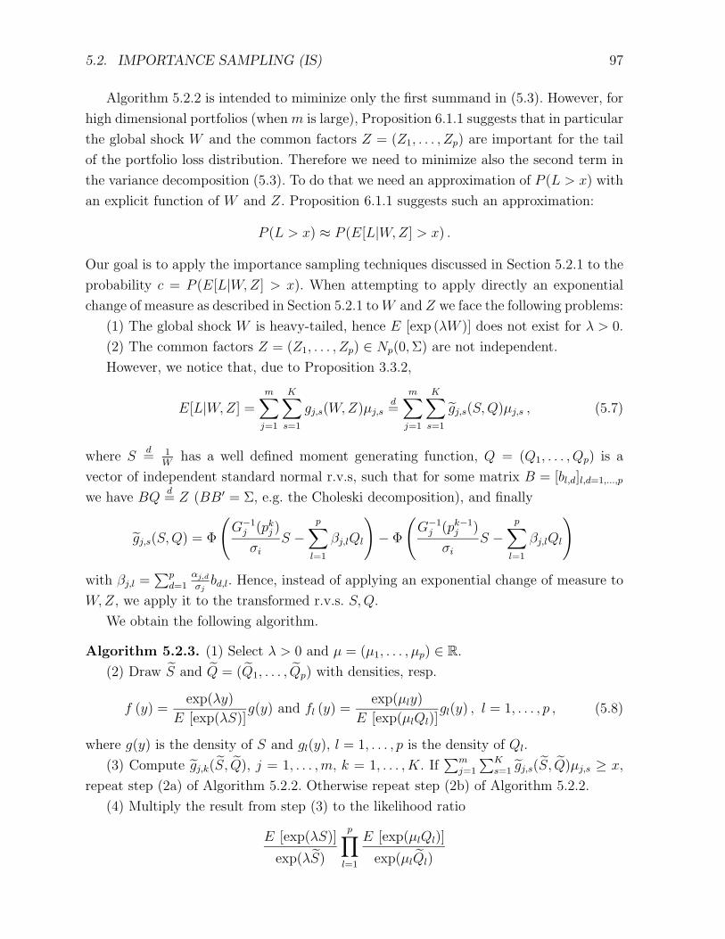
5.2. IMPORTANCE SAMPLING (IS) 97
Algorithm 5.2.2 is intended to miminize only the first summand in (5.3). However, for
high dimensional portfolios (when m is large), Proposition 6.1.1 suggests that in particular
the global shock W and the common factors Z = (Z1, . . . , Zp) are important for the tail
of the portfolio loss distribution. Therefore we need to minimize also the second term in
the variance decomposition (5.3). To do that we need an approximation of P (L > x) with
an explicit function of W and Z. Proposition 6.1.1 suggests such an approximation:
P (L > x) ≈ P (E[L|W,Z] > x) .
Our goal is to apply the importance sampling techniques discussed in Section 5.2.1 to the
probability c = P (E[L|W,Z] > x). When attempting to apply directly an exponential
change of measure as described in Section 5.2.1 toW and Z we face the following problems:
(1) The global shock W is heavy-tailed, hence E [exp (λW )] does not exist for λ > 0.
(2) The common factors Z = (Z1, . . . , Zp) ∈ Np(0,Σ) are not independent.
However, we notice that, due to Proposition 3.3.2,
E[L|W,Z] =m∑j=1
K∑s=1
gj,s(W,Z)µj,sd=
m∑j=1
K∑s=1
gj,s(S,Q)µj,s , (5.7)
where Sd= 1
Whas a well defined moment generating function, Q = (Q1, . . . , Qp) is a
vector of independent standard normal r.v.s, such that for some matrix B = [bl,d]l,d=1,...,p
we have BQd= Z (BB′ = Σ, e.g. the Choleski decomposition), and finally
gj,s(S,Q) = Φ
(G−1j (pkj )
σiS −
p∑l=1
βj,lQl
)− Φ
(G−1j (pk−1
j )
σiS −
p∑l=1
βj,lQl
)
with βj,l =∑p
d=1αj,dσjbd,l. Hence, instead of applying an exponential change of measure to
W,Z, we apply it to the transformed r.v.s. S,Q.
We obtain the following algorithm.
Algorithm 5.2.3. (1) Select λ > 0 and µ = (µ1, . . . , µp) ∈ R.
(2) Draw S and Q = (Q1, . . . , Qp) with densities, resp.
f (y) =exp(λy)
E [exp(λS)]g(y) and fl (y) =
exp(µly)
E [exp(µlQl)]gl(y) , l = 1, . . . , p , (5.8)
where g(y) is the density of S and gl(y), l = 1, . . . , p is the density of Ql.
(3) Compute gj,k(S, Q), j = 1, . . . ,m, k = 1, . . . , K. If∑m
j=1
∑Ks=1 gj,s(S, Q)µj,s ≥ x,
repeat step (2a) of Algorithm 5.2.2. Otherwise repeat step (2b) of Algorithm 5.2.2.
(4) Multiply the result from step (3) to the likelihood ratio
E [exp(λS)]
exp(λS)
p∏l=1
E [exp(µlQl)]
exp(µlQl)
98 CHAPTER 5. SIMULATION
to obtain an estimate for P (L > x)
(5) Average over N independent draws.
Step (2) of the above algorithm is comparatively easy to perform. In particular, by (5.8)
Q is a vector of independent normals with mean µ. In the most frequently used in practice
heavy-tailed t-model (see Example 3.2.1), S2 has a gamma d.f., see e.g. Glasserman et
al. [69], who apply a similar techique to the simulation of a market risk model with heavy-
tailed risk factors. For the selection of the design parameters λ and µ1, . . . , µp in step (1)
we apply the method in (5.2), i.e. we select
µ = arg min(λ,µ)
(E [exp(λS)]
exp(λq0(λ, µ))
p∏l=1
E [exp(µlQl)]
exp(µlql(λ, µ))
),
where q(λ, µ) = (q0(λ, µ), . . . , qp(λ, µ)) satisfy
q(λ, µ)) = arg maxq
(λq0 +
p∑l=1
µlql |E[L |S = q0, Q = (q1, . . . , qp)] = x) .
Due to (5.7) and (5.8) this choice guarantees, for instance, that
E[L |W = 1/E[S], Z = BE[Q]] = x ,
i.e. losses equal or exceeding x are no longer rare under the twisted probability measure.
5.3 Numerical examples
5.3.1 Comparison of the methods
We consider an example to demonstrate the suggested importance sampling method for
a credit portfolio with heavy-tailed risk factors.
Example 5.3.1. [IS for 10 factors and global shock portfolio]
The parameters of the considered model (as in (3.1) with (3.4) and (3.5)) are as follows:
- m = 100 credits in the portfolio;
- the exposures e = (e1, . . . , em) are generated uniformly on the interval (1, 25);
- rating system with K = 2 ratings (default and non-default);
- the default probabilities P (Xj = 1) = pj,1, j = 1, . . . ,m, are generated uniformly on
the interval [0.001, 0.02];
- the marginal loss distributions are given as Lj = 1Xj=1, j = 1, . . . ,m.
For the dependence structure we use in (3.5) the t-model with ν = 4 degrees of freedom,
p = 21 common factors and Z ∈ Np(0, I). The factor loadings are given, for j = 1, . . . ,m,
5.3. NUMERICAL EXAMPLES 99
by αj,1 = 0.7, αj,l = 0.3, l = jmod 10 + 1 and αj,l = 0.3, l = [j/10] + 11 ([x] denotes
the closest integer smaller than x). Thus, each credit has a loading of 0.7 on the first
factor and loadings 0.3 on two of the next. There are no equivalent credits with respect to
the dependence structure. The first factor may be thought of as a global factor, the next
ten as regional factors and the last ten as industry factors. This multifactor dependence
structure is taken from Glasserman [67], where it is described as particularly hard to deal
with.
200 400 600 800 100010
−5
10−4
10−3
10−2
10−1
Loss level
Tai
l pro
babi
lity
Monte Carloupper conf. boundlower conf. boundMonte Carlo + ISIS upper conf. boundIS lower conf. bound
200 400 600 800 100010
−5
10−4
10−3
10−2
10−1
Loss level
Tai
l pro
babi
lity
Monte Carloupper conf. boundlower conf. boundMonte Carlo + ISIS upper conf. boundIS lower conf. bound
Figure 5.1: The parameters are the same as in Example 5.3.1.Left figure: The tail of the portfolio loss distribution obtained by 10 000 Monte Carlo simulations of allrandom components of L compared to the tail obtained by Algorithm 5.2.2 with the same computationaltime budget, together with their respective 90% confidence bounds. The tightening of the confidencebounds, in particular at the extremely high loss levels (800-1000), is not sufficient enough.Right figure: The tail of the portfolio loss distribution obtained by 10 000 Monte Carlo simulations of allrandom components of L compared to the tail obtained by Algorithm 5.2.3 with the same computationaltime budget, together with their respective 90% confidence bounds. The tightening of the confidencebounds is now quite satisfactory.
We first simulate N = 10000 i.i.d copies of the portfolio loss L using the standard Al-
gorithm 5.1.1. As expected, this method produces rather broad confidence bounds at high
loss levels. In order to analyse if there is a room for improvement, we fix the computational
time required by Algorithm 5.1.1 and apply Algorithm 5.2.2, i.e. we use straightforward
simulation of the global shock W and the common factors Z1, . . . , Zp, combined with
(conditional) IS for the marginal losses. In Figure 5.1 (left) we observe that in this way
we obtain better confidence bounds, however, there is less improvement at extremely high
loss levels. For this reason, with the same fixed computational time, we apply also Algo-
rithm 5.2.3, i.e. we use combined IS for the global shock W , the common factors Z1, . . . , Zp
and the marginal losses. In Figure 5.1 (right) we observe that in this way we may obtain
narrow confidence bounds also at extremely high confidence levels.
100 CHAPTER 5. SIMULATION
5.3.2 Comparison of the models
From the examples and the analysis in Section 3.2, we expect that the heavy tailed risk
factors Y in model (3.5) will have a significant impact on the tail of the credit portfolio
loss distribution. We demonstrate this in the following example, see Frey et al. [62] or
Schwarz [131] for more examples.
Example 5.3.2. [Example 3.2.4 continued, comparison of the impact on the tail]
We consider 6 different portfolios L[1], . . . , L[6] with parameters, for each portfolio, as in
model (as in (3.1) with (3.4) and (3.5)) as follows:
- m = 100 credits in the portfolio;
- the exposures e = (e1, . . . , em) are generated uniformly on the interval (1, 25);
- rating system with K = 2 ratings (default and non-default);
- the default probabilities P (Xj = 1) = p[k], j = 1, . . . ,m, where p[k] is the default
probability for the credits of group Rk, k = 1, . . . , 6, as in Example 3.2.4;
- the marginal loss distributions are given as Lj = 1Xj=1, j = 1, . . . ,m.
The dependence structure is as in Example 3.2.4. More precisely, we compare a one-
factor CreditMetrics model (W = 1 a.s. in (3.5)) to a heavy-tailed t-model (Example 3.2.1)
with ν = 4 degrees of freedom and equal correlation structure.
In Figure 5.2 we compare the tails for the 6 portfolios L[1], . . . , L[6] under the Gaussian
and under the heavy-tailed dependence assumptions. In all cases, the heavy-tailed model
leads to higher risk as measured by, e.g. a high quantile of the loss distribution. It is
particularly apparent for portfolios L[1], L[2] (good quality obligors), see the upper row of
Figure 5.2 (recall our forecasts in Example 3.2.4).
Finally we consider the portfolio L =∑6
k=1 L[k] and its high α-quantile VaRα(L). It
is often assumed in practice that∑6
k=1 VaRα(L[k]) provides a conservative upper bound
for VaRα(L), although this is theoretically wrong, see Embrechts et al. [45] for a detailed
discussion on this issue. Our simple example demonstrates that the sum of the VaRs for
the 6 portfolios under the normal model assumption is significanly smaller than the total
portfolio VaR in the heavy-tailed case, see Figure 5.3. Clearly, it is hopeless to obtain a
conservative upper bound on the portfolio risk using simplified models and theoretically
unmotivated ”shortcuts”.
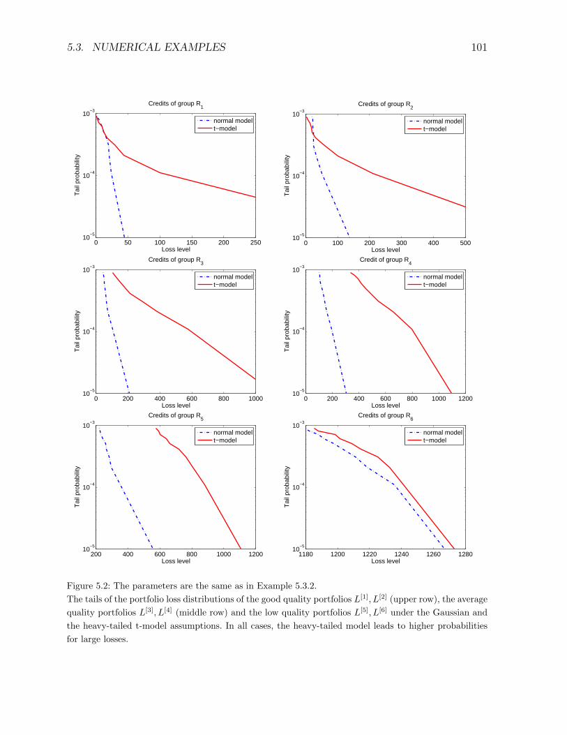
5.3. NUMERICAL EXAMPLES 101
0 50 100 150 200 25010
−5
10−4
10−3
Loss level
Tai
l pro
babi
lity
Credits of group R1
normal modelt−model
0 100 200 300 400 50010
−5
10−4
10−3
Credits of group R2
Loss level
Tai
l pro
babi
lity
normal modelt−model
0 200 400 600 800 100010
−5
10−4
10−3
Credits of group R3
Loss level
Tai
l pro
babi
lity
normal modelt−model
0 200 400 600 800 1000 120010
−5
10−4
10−3
Credit of group R4
Loss level
Tai
l pro
babi
lity
normal modelt−model
200 400 600 800 1000 120010
−5
10−4
10−3
Credits of group R5
Loss level
Tai
l pro
babi
lity
normal modelt−model
1180 1200 1220 1240 1260 128010
−5
10−4
10−3
Credits of group R6
Loss level
Tai
l pro
babi
lity
normal modelt−model
Figure 5.2: The parameters are the same as in Example 5.3.2.The tails of the portfolio loss distributions of the good quality portfolios L[1], L[2] (upper row), the averagequality portfolios L[3], L[4] (middle row) and the low quality portfolios L[5], L[6] under the Gaussian andthe heavy-tailed t-model assumptions. In all cases, the heavy-tailed model leads to higher probabilitiesfor large losses.
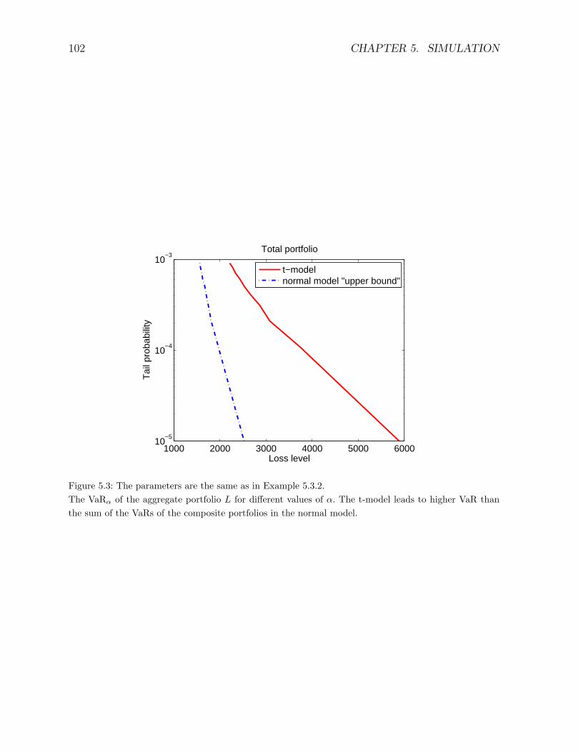
102 CHAPTER 5. SIMULATION
1000 2000 3000 4000 5000 600010
−5
10−4
10−3
Total portfolio
Loss level
Tai
l pro
babi
lity
t−modelnormal model "upper bound"
Figure 5.3: The parameters are the same as in Example 5.3.2.The VaRα of the aggregate portfolio L for different values of α. The t-model leads to higher VaR thanthe sum of the VaRs of the composite portfolios in the normal model.
Chapter 6
Tail approximation
For many applications in risk management, a fast evaluation of the tail of the credit port-
folio loss distribution is needed. As already noted (see CreditMetrics [74]), it is not possible
to obtain the distribution analytically even in the simplest Gaussian copula model. The
Monte Carlo simulation methods described in Chapter 5, even when enhanced with the
appropriate variance reduction techniques, are not the universal answer. In particular
when the goal is to perform a sensitivity analysis for some of the model parameters, an
analytic approximation is more suited.
Various approximations of the portfolio loss distribution have been developed. Most
of them are based on the SLLN or on the CLT, see Section 6.1. The required granularity
assumptions for these approximations (see e.g. Bluhm et al. [16], Assumption 2.5.2) are not
always easy to verify in practice. Furthermore, such approximations are typically accurate
at the center of the distribution (close to the mean) and could be misleading in the tail.
In contrast, we consider an approximation based on the large deviations theory, which
is designed to be accurate in the tail. More precisely, we apply the Markov’s inequality
to derive an upper bound of exponential type for the tail of L. In order to compute the
best possible (the closest to the tail) upper bound, we develop a stochastic approximation
algorithm and show its a.s. convergence to the optimal bound. This algorithm turns out to
be a useful tool for risk management applications in Chapter 7. Before that we illustrate
its accuracy and computational efficiency by a numerical example in Section 6.3.
6.1 Approximation for large portfolios
The approximations which are currently used in practice rely on two facts:
(1) Given a set of factors, the individual transactions in a credit portfolio are indepen-
dent (see Gordy [71] for general credit risk models or Finger [52] for the CreditMetrics
model in particular).
103
104 CHAPTER 6. TAIL APPROXIMATION
(2) The portfolio consists of a large number of comparatively homogeneous obligors.
More precisely, we consider the asymptotic distribution of the sequence of portfolios
L(m) satisfying (3.1) with (3.4) and (3.5) for the number of obligors m going to infinity.
We need the following additional ’granularity’ assumptions on the obligors’ exposures:
limm→∞
m∑j=1
ej =∞ , (6.1)
limm→∞
m∑j=1
(ej∑ji=1 ei
)2
<∞ , (6.2)
Cj ≥ C, j ∈ N , (6.3)
where Cj are the constants from Assumption (C) in (3.1) and C ∈ R is a fixed constant.
Assumption (6.1) guarantees that the total portfolio exposure increases to infinity as
the number of obligors increases to infinity. This holds, for instance, when ej ≥ a, j ∈ N,
for some constant a > 0. Assumption (6.2) implies that the exposure weights shrink
rapidly with increasing number of obligors. This holds, for instance, when ej ∈ [a, b], j ∈ Nfor some constants 0 < a ≤ b < ∞. Assumption (6.3) guarantees that no credit in the
portfolio could lead to a profit larger than |C|ej, j ∈ N.
A less general version of the proposition below is for instance Bluhm et al. [16], Propo-
sition 2.5.4. We prove it in our general setting.
Proposition 6.1.1. Let L(m) be a sequence of rvs with distributions as in (3.1) with (3.4)
and (3.5). Let also (6.1), (6.2) and (6.3) hold and denote by τm =∑m
j=1 ej. Then
1
τm(L(m) − E
[L(m) |W,Z
])
a.s.→ 0, m→∞. (6.4)
Proof. We note first that, due to (3.5), given W and Z, the r.v.s Yj, j = 1, . . . ,m, are
independent (inherited by the independence of εj). Therefore Xj, j = 1, . . . ,m, are condi-
tionally (on W and Z) independent by means of (3.4). Therefore, due to assumption (A)
in (3.1), the r.v.s ξj = ej(Lj−E[Lj |W,Z]) are (conditionally) independent. Furthermore,
E[ξj] = 0 by definition. Finally, due to assumption (C) in (3.1) and (6.3), condition (6.2)
leads to
limm→∞
m∑j=1
E[ξ2j ]
(τj)2≤ lim
m→∞
m∑j=1
4 max(1, |C|)2e2j
(τj)2<∞ ,
where E denotes the expectation under the conditional on W and Z probability measure.
Applying the SLLN we obtain
P ( limm→∞
1
τm(L(m) − E[L(m) |W,Z]) = 0 |W = w,Z = z) = 1 ,
for every w > 0 and z ∈ Rd. Integrating w.r.t. W and Z we obtain the required result.
6.2. APPROXIMATION BY AN UPPER BOUND 105
6.2 Approximation by an upper bound
In order to obtain an upper bound of the portfolio loss distribution we apply Markov’s
inequality: for every θ ≥ 0 and x ∈ [E [L] , Lmax)
P (L ≥ x) ≤ E [exp (θ (L− x))] = ϕ (θ) exp (−θx) =: F (θ, x) . (6.5)
In the next lemma we summarize some of the important properties of F (θ, x).
Lemma 6.2.1. Let x ∈ (E [L] , Lmax) be fixed. Then the function F (θ, x) satisfies the
following properties.
(1) F (θ, x) is analytic in θ;
(2) there exists a unique positive point
θ = θ (x) = arg minθF (θ, x) , (6.6)
which is the unique positive solution of the equation ∂∂θF (θ, x) = 0;
(3) F (θ, x) is strictly decreasing for θ < θ(x) and strictly increasing for θ > θ(x);
(4) F (θ, x)→∞, θ →∞;
(5) θ (x) ∈ (0, θmax(x)), where θmax(x) <∞ satisfies F (θmax(x), x) = 1;
(6) there exist constants D(x) ≥ C(x) > 0 such that for all θ, 0 < θ <∞, θ 6= θ
C(x) ≤∂∂θF (θ, x)
θ − θ≤ D(x) . (6.7)
Proof. Properties (1), (2) and (3) are standard (see e.g. Jensen [82], section 1.2 and
references therein).
As x < Lmax, there exists ε > 0 such that x+ ε < Lmax and hence P (L > x+ ε) > 0,
therefore
limθ→∞
F (θ, x) ≥ limθ→∞
P (L > x+ ε) exp(θε) =∞ ,
i.e. we get (4).
By (2) we have 0 < θ(x). Note that F (0, x) = 1 for every x, hence, due to (3),
F (θ(x), x) < 1. As F (θ, x) is continuous in θ, by means of (4) there exists a point 0 <
θmax(x) < ∞ which satisfies F (θmax(x), x) = 1. Because of (3), we get θ(x) < θmax(x),
i.e. (5).
To prove (6) we use a Taylor expansion of ∂∂θF (θ, x) around θ and the fact that
∂∂θF (θ, x) = 0; we get for ε = ε(θ) ∈ (min(θ, θ),max(θ, θ))
∂∂θF (θ, x)
θ − θ=
∂2
∂θ2F (ε, x) .
106 CHAPTER 6. TAIL APPROXIMATION
For θ ∈ R we have
∂2
∂θ2F (θ, x) =
∂2
∂θ2E [exp (θ (L− x))]
= E[(L− x)2 exp (θ (L− x))
]> 0 .
Also, by means of (3.7),
∂2
∂θ2F (θ, x) ≤ (max(|Lmin|, Lmax) + |x|)2 exp (θ (Lmax − x)) <∞ .
As by (1) ∂2
∂θ2F (θ, x) is continuous in θ, for ε in a compact subset of R the function∂2
∂θ2F (ε, x) achieves a minimum and a maximum at some points εmin and εmax, which are
strictly positive, hence there exist positive constants C(x) and D(x) such that
0 < C(x) ≤ ∂2
∂θ2F (εmin, x) ≤
∂∂θF (θ, x)
θ − θ≤ ∂2
∂θ2F (εmax, x) ≤ D(x) <∞ .
To derive a best upper bound of P (L ≥ x) we calculate the saddlepoint θ as defined
in (6.6) and we obtain
P (L ≥ x) ≤ F (θ, x), x ∈ (E[L], Lmax) (6.8)
This classical large deviations technique has been successfully applied by Martin et
al. [109] in the case of a one-factor Gaussian model (p = 1, W = 1 in (3.5)). Unfortunately
in our case it is not possible to compute θ explicitly or by simple numerical methods, since
the moment generating function ϕ (θ) is available only in terms of the (p+1)-dimensional
integral (3.8). As a remedy we develop a Monte Carlo estimator for the saddlepoint θ and
at the same time we obtain an estimator for the best upper bound F (θ, x) in (6.8).
The proposed method is in the framework of stochastic approximation algorithms
(see Kushner and Yin [96]). More precisely, we approximate the saddlepoint θ, for fixed
x ∈ (E[L], Lmax), by simulating recursively the r.v.s:
θn+1 = θn − anTn, n ∈ N ,
where θ1 is an arbitrary positive number,
Tn =∂
∂θexp
(H(W (n), Z(n), θn
)− θnx
)(6.9)
and W (n) and Z(n) are i.i.d. copies of W and Z, respectively, an, n∈N is a sequence of
positive constants such that
6.2. APPROXIMATION BY AN UPPER BOUND 107
∞∑n=1
an =∞ (6.10)
∞∑n=1
a2n = A2 <∞ (6.11)
limn→∞
an = 0 , (6.12)
and H(W,Z, θ) is defined in (3.9).
In the next theorem we prove that (a modification of) θna.s.→ θ. The modification is
taken in order to ensure ’stability’ of the algorithm, i.e. to avoid θn growing to infinity
for some ω ∈ Ω, see Kushner and Yin [96], Section 5.1 for details. Usually in stochastic
approximation algorithms stability is achieved by assuring that each iterate θn belongs to
some compact set which includes the true value θ. In our case this compact set is given
by [0, θmax(x)], where θmax(x) is the constant from Lemma 6.2.1 (5). Since the constant
θmax(x) is not explicitly available, we approximate it by a sequence of r.v.s converging
a.s. to it.
Theorem 6.2.2. Let x ∈ (E [L] , Lmax) be fixed. For n ∈ N let T(i)n , i ∈ N, be i.i.d copies
of the r.v. defined in (6.9). Let an, n∈N be a sequence of positive constants satisfying (6.10),
(6.11) and (6.12). Define
θn+1 = mini
θ
(i)n+1 = θn − anT (i)
n : 0 ≤ θ(i)n+1 ≤ Kn
, (6.13)
where
Kn = supθθ : Fn (θ, x) ≤ 1
with Fn (θ, x) being the empirical counterpart of F (θ, x) as defined in (6.5)
Fn (θ, x) =1
n
n∑i=1
exp(H(W (i), Z(i), θ
)− θx
). (6.14)
Then
θna.s.→ θ, n→∞.
Proof. Step 1: We prove that θn is finite a.s. for every n ∈ N.
First we prove by induction that θn < ∞ for any fixed n. We have θ1 < ∞. Assume
that θn <∞. Note that
|Tn| = | ∂∂θH (W,Z, θn)− x| exp (H (W,Z, θn)− θnx) .
108 CHAPTER 6. TAIL APPROXIMATION
However, since θn ≥ 0 by means of (6.13), exp (H (W,Z, θn)) ≤ exp(θnLmax) because of
(3.7); and also by (3.9)
| ∂∂θH (W,Z, θn) | ≤
m∑j=1
| ∂∂θ
logHj (W,Z, θ) |
=m∑j=1
|ejE [Lj exp(θnejLj) |W,Z]
E [exp(θnejLj) |W,Z]|
≤m∑j=1
ej max(1, |Cj|) exp(θnej)
exp(θnejCj)
by means of assumption (C) in (3.1). Therefore
|Tn| ≤ K(θn) , (6.15)
where K(θn) is finite if θn is finite. Therefore, by means of (6.13) and (6.15), θn+1 is also
finite for a finite n.
Now assume that for some ω ∈ Ω θn →∞, n→∞. By the SLLN we have for θ ∈ R
Fn (θ, x)a.s.→ E [exp (θ (L− x))] = F (θ, x) .
Furthermore, F (θ, x) is continuous in θ and Fn (θ, x) is a.s. continuous in θ and, by
means of Lemma 6.2.1 (4), F (θ, x) → ∞ when θ → ∞. So have for this ω and for some
sufficiently large n that Fn (θn, x) > 1. Such a value of θn is excluded by (6.13). Hence θn
is finite a.s.
Step 2: We prove that
(θn − θ)2 a.s.→ γ, n→∞ ,
where γ is some r.v. with finite mean.
Denote by Fn = σ(θ1, . . . , θn,W(1), Z(1), . . . ,W(n−1), Z(n−1)
), where W(j), Z(j) are the
realizations for which θj+1 = θj−ajT (i)j . Denote Tj = T
(i)j . From (6.13) we have θn+1− θ =
θn − θ − anTn, hence
E[(θn+1 − θ)2 | Fn
]= (θn − θ)2 + a2
nE[T 2n | Fn
]− 2anE
[Tn(θn − θ) | Fn
]. (6.16)
Consider first
E[Tn(θn − θ) | Fn
]= (θn − θ)E [Tn | Fn]
= (θn − θ)E [Tn | θn]
= (θn − θ)∂
∂θE[exp
(H(W(n), Z(n), θn
)− θnx
)| θn]
= (θn − θ)∂
∂θF (θn, x) .
6.2. APPROXIMATION BY AN UPPER BOUND 109
Secondly,
n∑k=1
a2kE[T 2k | Fk
]=
n∑k=1
a2kE[T 2k | θk
]≤
∞∑k=1
a2kE[T 2k | θk
]≤ K2A2 , (6.17)
where A2 is the limiting constant from (6.11) and K2 <∞ is a constant, independent of
θk, such that
E[T 2k | θk
]≤ K2 (6.18)
for every k ∈ N (the existence of such a constant follows from Step 1 and (6.15)).
Denote
Mn+1 = (θn+1 − θ)2 +K2A2 −n∑k=1
a2kE[T 2k | θk
].
From (6.17) we know that Mn ≥ 0. On the other hand, using (6.16),
E [Mn+1 | Fn] = E[(θn+1 − θ)2 | Fn
]+K2A2 −
n∑k=1
a2kE[E[T 2k | θk
]| Fn
]= Mn − 2anE
[Tn(θn − θ) | Fn
]= Mn − 2an(θn − θ)
∂
∂θF (θn, x) .
By means of (6.7) (θn−θ) ∂∂θF (θn, x) > 0 a.s., hence Mn is a non-negative supermartingale.
By Doob’s limit theorem
Mna.s.→ M, n→∞, (6.19)
where M is a r.v. with finite mean. As K2A2 is some constant and∑n
k=1 a2kE [T 2
k | θk] is an
increasing, but bounded by means of (6.17) sequence, (6.19) implies that (θn − θ)2 a.s.→ γ,
where γ is a r.v. with finite mean.
Step 3. Denote ηn = E (θn− θ)2. We prove that there exists n1 ∈ N such that for every
n > n1
ηn+1 ≤ (1− anC)2 ηn + a2nK
2 , (6.20)
where C is the constant from (6.7) and K is the constant from (6.18).
Denoting Tn = Tn − ∂∂θF (θn, x) we obtain from (6.13)
θn+1 − θ = θn − θ − anTn − an∂∂θF (θn, x)
θn − θ(θn − θ)
=
(1− an
∂∂θF (θn, x)
θn − θ
)(θn − θ)− anTn .

110 CHAPTER 6. TAIL APPROXIMATION
Raising to second power and integrating we get
ηn+1 ≤ E
(1− an∂∂θF (θn, x)
θn − θ
)2
(θn − θ)2
− 2anE
[(1− an
∂∂θF (θn, x)
θn − θ
)(θn − θ)Tn
]+a2
nET2n .
Conditioning on Fn we have
E[(
1− an∂∂θF (θn,x)
θn−θ
)(θn − θ)Tn
]= E
[E
[(1− an
∂∂θF (θn, x)
θn − θ
)(θn − θ)Tn | Fn
]]
= E
[(1− an
∂∂θF (θn, x)
θn − θ
)(θn − θ)E
[Tn | Fn
]]
= E
[(1− an
∂∂θF (θn, x)
θn − θ
)(θn − θ)E
[Tn | θn
]]= 0 ,
because E[Tn | θn
]= E [Tn | θn]− E
[∂∂θF (θn, x) | θn
]= 0 a.s..
Due to (6.7) we have
1− an∂∂θF (θn, x)
θn − θ≤ 1− anC.
Also, since an converges to 0 and∂∂θF (θn,x)
θn−θ≥ D as in (6.7), we can always select an index
n1, such that an <1D
for every n > n1, and hence 1− an∂∂θF (θn,x)
θn−θ> 0. We get
ηn+1 ≤ (1− anC)2 ηn + a2nET
2n .
Since ET 2n = E
(Tn − ∂
∂θF (θn, x)
)2= var[Tn] ≤ ET 2
n ≤ K2 we obtain (6.20).
Step 4. Finally we prove that
limn→∞
ηn = 0. (6.21)
Since a.s. convergence implies convergence in probability, by means of Step 2 we have
limn→∞
ηn = Eγ <∞.
On the other hand, since γ = limn→∞(θn − θ)2 is a non-negative r.v., showing (6.21) is
enough to prove the theorem.
We have by (6.20), for every sufficiently large n > n1,
√ηn+1 ≤ (1− anC)
√ηn + anK .
6.2. APPROXIMATION BY AN UPPER BOUND 111
We also have from Step 2 that limn→∞√ηn =
√Eγ. Now assume that
√Eγ > K
C. This
implies for some ε > 0√ηn ≥ K
C+ ε, for n > n2 = n2(ε). Let n2 > n1. We get
√ηn+1 ≤
√ηn − anC(
K
C+ ε) + anK
=√ηn − anCε .
Using the inequality recursively we get
n∑j=n2+1
(√ηj+1 −
√ηj)≤ −Cε
n∑j=n2+1
aj ,
which means√ηn+1 ≤
√ηn2 − Cε
n∑j=n2+1
aj .
However, due to (6.10), there exists some index n3, such that
√ηn2
Cε<
n3∑j=n1+1
aj ,
hence√ηn3 < 0, which is a contradiction. Therefore we obtain Eγ ≤ K2
C2 . Hence there
exists n4 ∈ N such that for n > n4 ηn ≤ K2
C2 .
Going back to (6.20), we have for sufficiently large n > max (n1, n4)
ηn+1 ≤ (1− anC)2 ηn + a2nK
2
= ηn + a2nC
2ηn − 2anCηn + a2nK
2
≤ ηn + a2nC
2K2
C2− 2anCηn + a2
nK2
= ηn − 2anCηn + 2a2nK
2
Assume the contrary to the hypothesis, that ηn > ε > 0 for every n larger than some fixed
n5. Then we get
ηn+1 ≤ ηn − 2anCε+ 2a2nK
2 .
Applying the inequality recursively we obtain
n∑j=n5+1
(ηj+1 − ηj) ≤n∑
j=n5+1
2a2jK
2 − 2Cεn∑
j=n5+1
aj
and therefore
ηn+1 ≤ ηn5 + 2K2
n∑j=n5+1
a2j − 2Cε
n∑j=n5+1
aj
≤ ηn5 + 2K2
∞∑j=1
a2j − 2Cε
n∑j=n5+1
aj .
112 CHAPTER 6. TAIL APPROXIMATION
However, due to (6.10), there exists some index n6, such that
ηn5 + 2K2A
2Cε<
n6∑j=n5+1
aj ,
hence ηn6+1 < 0, which is a contradiction. Therefore we obtain the required result.
Next we derive an approximation of the optimal upper bound F (θ, x) of P (L ≥ x) as
defined in (6.8).
Proposition 6.2.3. Let x ∈ (E [L] , Lmax) be fixed. For θ ∈ R let Fn (θ, x) be defined as
in (6.14). If θna.s.→ θ, n→∞, then
Fn(θn, x)a.s.→ F (θ, x), n→∞ (6.22)
Proof. By the SLLN we have
Fn (θ, x)a.s.→ E [exp (θ (L− x))] = F (θ, x)
for every θ ∈ R. As exp(H(W (i), Z(i), θ)− θx
)and F (θ, x) are a.s. continuous in θ and
θna.s.→ θ, by the continuous mapping theorem we have
Fn(θn, x)a.s.→ F (θ, x), n→∞.
Remark 6.2.4. At each simulation step of (6.13), we check if Fn (θn, x) < 1. Therefore,
the upper bound approximation of P (L ≥ x) is available as by-product from the proposed
algorithm.
6.3 Numerical examples
We give an example to demonstrate our method.
Example 6.3.1. [Example 5.3.1 continued, tail approximation]
We consider model (3.1) with (3.4) and (3.5) and the parameters from Example 5.3.1.
In Figure 6.1 (left) we compare the tail of the portfolio loss distribution, obtained by Monte
Carlo simulation as explained in Section 5.1 to the upper bound approximation as in (6.8),
obtained by the new method (6.22). We observe that the upper bound approximation is
quite accurate at high loss levels (i.e. 500-800), but degenerates quickly as we move in
direction to the mean of the distribution. Furthermore, by the new approximation method
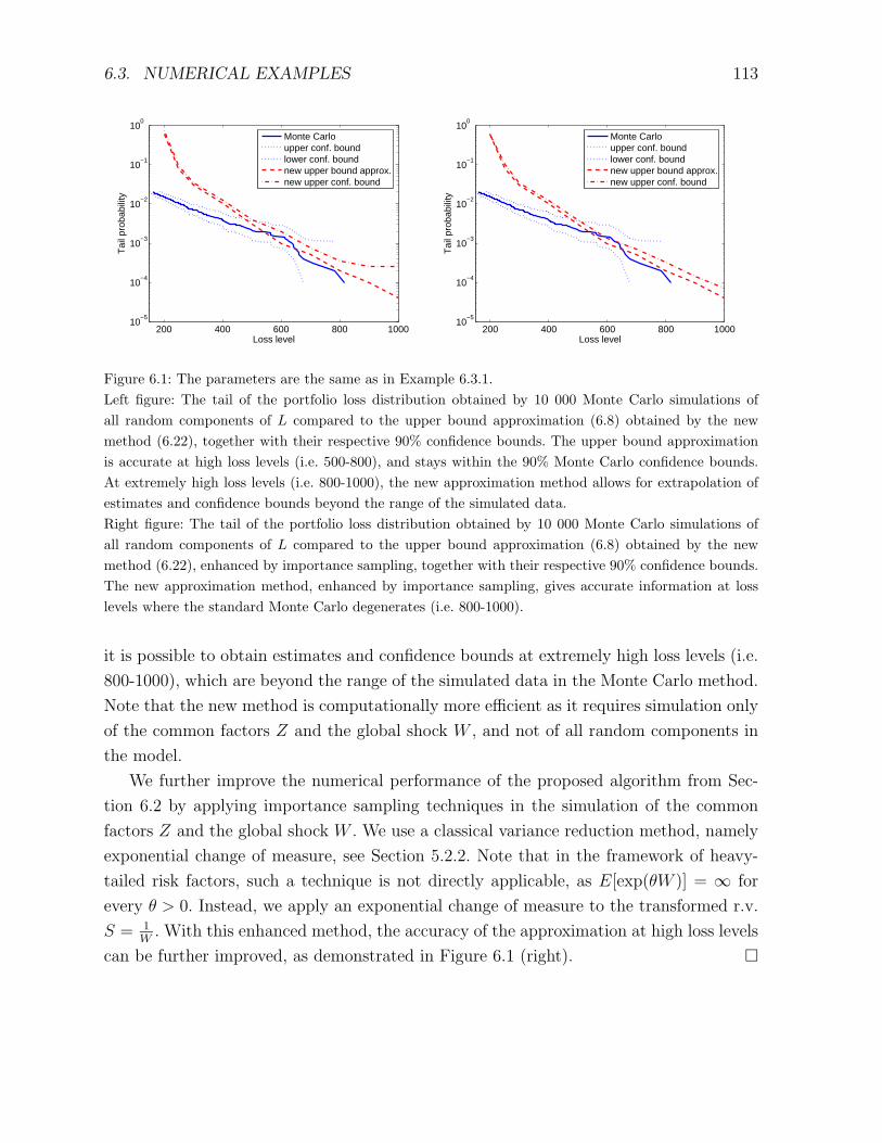
6.3. NUMERICAL EXAMPLES 113
200 400 600 800 100010
−5
10−4
10−3
10−2
10−1
100
Loss level
Tai
l pro
babi
lity
Monte Carlo upper conf. boundlower conf. boundnew upper bound approx.new upper conf. bound
200 400 600 800 100010
−5
10−4
10−3
10−2
10−1
100
Loss level
Tai
l pro
babi
lity
Monte Carloupper conf. boundlower conf. boundnew upper bound approx.new upper conf. bound
Figure 6.1: The parameters are the same as in Example 6.3.1.Left figure: The tail of the portfolio loss distribution obtained by 10 000 Monte Carlo simulations ofall random components of L compared to the upper bound approximation (6.8) obtained by the newmethod (6.22), together with their respective 90% confidence bounds. The upper bound approximationis accurate at high loss levels (i.e. 500-800), and stays within the 90% Monte Carlo confidence bounds.At extremely high loss levels (i.e. 800-1000), the new approximation method allows for extrapolation ofestimates and confidence bounds beyond the range of the simulated data.Right figure: The tail of the portfolio loss distribution obtained by 10 000 Monte Carlo simulations ofall random components of L compared to the upper bound approximation (6.8) obtained by the newmethod (6.22), enhanced by importance sampling, together with their respective 90% confidence bounds.The new approximation method, enhanced by importance sampling, gives accurate information at losslevels where the standard Monte Carlo degenerates (i.e. 800-1000).
it is possible to obtain estimates and confidence bounds at extremely high loss levels (i.e.
800-1000), which are beyond the range of the simulated data in the Monte Carlo method.
Note that the new method is computationally more efficient as it requires simulation only
of the common factors Z and the global shock W , and not of all random components in
the model.
We further improve the numerical performance of the proposed algorithm from Sec-
tion 6.2 by applying importance sampling techniques in the simulation of the common
factors Z and the global shock W . We use a classical variance reduction method, namely
exponential change of measure, see Section 5.2.2. Note that in the framework of heavy-
tailed risk factors, such a technique is not directly applicable, as E[exp(θW )] = ∞ for
every θ > 0. Instead, we apply an exponential change of measure to the transformed r.v.
S = 1W
. With this enhanced method, the accuracy of the approximation at high loss levels
can be further improved, as demonstrated in Figure 6.1 (right).

114 CHAPTER 6. TAIL APPROXIMATION
Chapter 7
Application to risk measurement
Today, virtually all major banks and financial institutions evaluate the risk-adjusted prof-
itability within various business lines, including credits. The key concept behind this risk-
adjusted performance measurement is described briefly in Section 7.1. The crucial point
is to compute the contribution of the marginal risky position (e.g. the marginal credit)
to the overall portfolio risk. Depending upon the choice of a risk measure, this could be a
straightforward or a quite complicated task in the credit risk model under consideration,
see Section 7.2.
The main result in this chapter is an application of the upper bound of the tail of the
portfolio loss as derived in Section 6.2 to risk measurement. The application is given in
Section 7.3. We define a new risk measure – tail bound VaR. We provide an algorithm
to compute this risk measure and the contribution of the marginal credits to it. In Sec-
tion 7.4.1 the risk contributions obtained by our method are compared to the Expected
Shortfall (ES) contributions suggested for instance in Overbeck [122]. We find out that
the two methods give similar results, however, our method has lower computational costs.
This opens up a way to investigate the impact of the different model assumptions (Gaus-
sian vs heavy-tailed) on the risk structure of the portfolio, as given by the marginal risk
contributions.
7.1 Risk-adjusted performance measurement
Suppose an investor wants to place a fixed amount of capital into some asset. He has two
exclusive choices: asset j, j = 1, 2, yields expected return mj with risk rj. Evidently, if
the risks are equal, he will choose the asset with the higher yield. In the case of different
risks (say r1 > r2) there is not such an obvious answer. No doubt that m1 should be larger
than m2 for asset 2 to be eligible at all. But how large should be the difference in order
to make asset 2 more attractive?
115
116 CHAPTER 7. APPLICATION TO RISK MEASUREMENT
The Markowitz portfolio theory (see [108]) is the classical reference for a solution to
this problem. It is still effective nowadays (see Becker et al. [11]). The investor should
decide in favor of asset 1 if and only if m1
r1≥ m2
r2. This kind of computing is commonly
called RORAC (return on risk-adjusted capital, see Matten [111]) and the comparison
procedure is called RAPM (risk-adjusted performance measurement).
Note that the Markowitz’s notion of risk is rather abstract. It is considered as a measure
of the uncertainty in return, and is defined mathematically as the standard deviation of
the return. Despite its computational convenience, this perspective has some drawbacks.
From the risk management point of view, it is not desirable that not only the unfavorable,
but also favorable fluctuations of the return around its mean have impact on the risk, as
it happens with the standard deviation. The way to handle this problem is clear: one has
to make use of down-sided risk measures, see Fishburn [54].
The down-sided risk measure Value-at-Risk (VaR) has nowadays become an industry
standard (see BIS [9]). VaR is defined as a (small) quantile of the return distribution.
In the case when the distributions of the returns are normal, the VaR method and the
Markowitz theory yield identical results. However, the normal distribution assumption
seems to be completely wrong for credit portfolios, see CreditMetrics [74]. Nonetheless,
for the sake of RAPM, CreditMetrics [74] use the standard deviation as a risk measure.
In view of model (3.1), a portfolio is represented by the vector e = (e1, . . . , em) ∈ Rm+of the exposures of the individual credits. Further, a risk measure is simply a differentiable
function r = r(e) : Rm+ → R. We present some examples in the next section. Following
Tasche [134], we define marginal risk contributions as the gradient of the risk measure, i.e.
A = (A1, . . . , Am) = ∇r(e). The goal of this chapter is to provide a computationally fea-
sible alternative to the use of the standard deviation as a risk measure. More precisely, we
are interested in computing the marginal risk contributions w.r.t. different risk measures.
Remark 7.1.1. Note that in the original CreditMetrics model, the risk contribution is
defined differently, namely Aj = r(e)− r(e(j)), where e(j) is the vector of exposures e with
0 in its j-th component. For the drawbacks of this approach see Tasche [134].
7.2 Risk contributions w.r.t. standard risk measures
A classical example for risk measure is the standard deviation, i.e.
rvar(e) =√
var(L(e)) ,
where L is the portfolio loss defined in (3.1). An expression for rvar(e) is available in (3.14).
Note that, once rvar(e) is computed for some e ∈ Rm+ , computing rvar(e′), e 6= e′ ∈ Rm+
7.2. RISK CONTRIBUTIONS W.R.T. STANDARD RISK MEASURES 117
is trivial. Furthermore, by Example 5.1. in Tasche [134], we have for the marginal risk
contribution of credit j, j = 1, . . . ,m
Avarj =
cov(Lj, L)√var(L)
.
Furthermore,
cov(Lj, L) =m∑l=1
elcov(Lj, Ll) ,
and therefore this quantity is available as a by-product from the computation of√
var(L).
This makes the covariance based risk contributions particularly attractive for high-dimensional
portfolios.
Another frequently used in practice risk measure is the VaR, defined as
VaR(e) = infxP (L(e) > x) ≤ α , (7.1)
for some small probability α. Note that, if L is normally distributed, then VaR(e) =
Φ−1(1− α)√
var(L), i.e. in such cases this quantity is available explicitly through (3.14).
Unfortunately in model (3.1) with (3.4) and (3.5) the d.f. of L is far from being nor-
mal. Therefore, VaR(e) can be obtained only by means of Monte Carlo simulation, see
CreditMetrics [74].
As shown in Tasche [134], under some regularity conditions, the marginal risk contri-
butions for VaR are
AVaRj = E [Lj |L = VaR] , j = 1, . . . ,m . (7.2)
It is extremely hard to compute these quantities even by Monte Carlo methods, see Bluhm
et. al. [16], Section 5.2.2.
An alternative risk measure for credit risk portfolios is used for instance in Over-
beck [122]. Denoting the expected shortfall
ES (e) = E [L(e) |L(e) ≥ VaR (e)] ,
one obtains for the marginal risk contributions
AESj = E [Lj |L ≥ VaR] , j = 1, . . . ,m , (7.3)
see Tasche [134]. This measure has many advantages in the credit risk framework, see
e.g. Frey and McNeil [60] or Bluhm et al [16], Section 5.2.3. Furthermore, it is possible
to compute marginal risk contributions AESj by Monte Carlo methods. More precisely,
let L(i), i = 1, . . . , n, (and resp. L(i)j , j = 1, . . . ,m,) be i.i.d copies of L (and resp. of
118 CHAPTER 7. APPLICATION TO RISK MEASUREMENT
Lj, j = 1, . . . ,m,) as in (3.1). Denote by Bn =i, i = 1, . . . , n : L(i) ≥ Ldαne
, where
Ldαne is the dαneth largest order statistic among L(i), i = 1, . . . , n. Then the SLLN
provides estimates for (7.3), i.e.
1
#Bn
∑i∈Bn
L(i)j
a.s.→ AESj , n→∞ .
7.3 Risk contributions w.r.t. tail bound VaR
In this section we explain how we use the upper bound approximation of the portfolio
loss derived in Section 6.2 to approximate the VaR and the marginal risk contributions
w.r.t. it. First we analyze the optimal upper bound F (θ(x), x) defined in (6.8), i.e.
F (θ(x), x) = ϕ(θ(x)) exp(−θ(x)x) ,
where ϕ (θ) is the moment generating function of L as in (3.8) and θ(x) is the saddlepoint
defined in (6.6).
Lemma 7.3.1. Let F (θ(x), x), x ∈ (E[L], Lmax), be the function defined in (6.8). Then
(1) θ (x) is continuous and strictly increasing in x;
(2) F (θ (x) , x) is continuous and strictly decreasing in x;
(3) the inverse function
VaR (α) = argx
F (θ(x), x) = α
, α ∈ (0, 1) (7.4)
is a well defined and strictly decreasing function;
(4) for every α ∈ (0, 1)
VaR (α) ≤ VaR (α) . (7.5)
Proof. To prove (1), taking into account that ∂∂θ
log(ϕ(θ (x))) = x (Lemma 6.2.1 (2)), we
get∂
∂x
∂
∂θlog(ϕ(θ (x))) = 1 ,
therefore ∂∂xθ (x) ∂2
∂θ2 log(ϕ(θ (x))) = 1. Hence ∂∂xθ (x) = ( ∂2
∂θ2 log(ϕ(θ (x))))−1 > 0 by the
strict convexity of ϕ(θ).
To prove (2) we note that log(F (θ (x) , x)) = log(ϕ(θ (x)))− θ (x)x. By differentiation
we get
∂
∂xlog(F (θ (x) , x)) =
∂∂θϕ(θ (x))
ϕ(θ (x))
∂
∂xθ (x)− x ∂
∂xθ (x)− θ (x)
=∂
∂xθ (x)
(∂∂θϕ(θ (x))
ϕ(θ (x))− x
)− θ (x)
= −θ (x) < 0
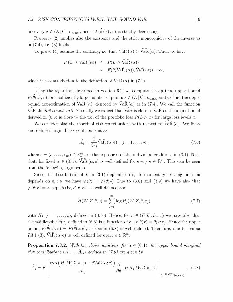
7.3. RISK CONTRIBUTIONS W.R.T. TAIL BOUND VAR 119
for every x ∈ (E [L] , Lmax), hence F (θ (x) , x) is strictly decreasing.
Property (2) implies also the existence and the strict monotonicity of the inverse as
in (7.4), i.e. (3) holds.
To prove (4) assume the contrary, i.e. that VaR (α) > VaR (α). Then we have
P (L ≥ VaR (α)) ≤ P (L ≥ VaR (α))
≤ F (θ(VaR (α)), VaR (α)) = α ,
which is a contradiction to the definition of VaR (α) in (7.1).
Using the algorithm described in Section 6.2, we compute the optimal upper bound
F (θ(x), x) for a sufficiently large number of points x ∈ (E [L] , Lmax) and we find the upper
bound approximation of VaR (α), denoted by VaR (α) as in (7.4). We call the function
VaR the tail bound VaR. Normally we expect that VaR is close to VaR as the upper bound
derived in (6.8) is close to the tail of the portfolio loss P (L > x) for large loss levels x.
We consider also the marginal risk contributions with respect to VaR (α). We fix α
and define marginal risk contributions as
Aj =∂
∂ejVaR (α; e) , j = 1, . . . ,m , (7.6)
where e = (e1, . . . , em) ∈ Rm+ are the exposures of the individual credits as in (3.1). Note
that, for fixed α ∈ (0, 1), VaR (α; e) is well defined for every e ∈ Rm+ . This can be seen
from the following arguments.
Since the distribution of L in (3.1) depends on e, its moment generating function
depends on e, i.e. we have ϕ (θ) = ϕ (θ; e). Due to (3.8) and (3.9) we have also that
ϕ (θ; e) = E[exp (H(W,Z, θ, e))] is well defined and
H(W,Z, θ, e) =m∑j=1
logHj(W,Z, θ, ej) (7.7)
with Hj, j = 1, . . . ,m, defined in (3.10). Hence, for x ∈ (E[L], Lmax) we have also that
the saddlepoint θ(x) defined in (6.6) is a function of e, i.e θ(x) = θ(x; e). Hence the upper
bound F (θ(x), x) = F (θ(x; e), x; e) as in (6.8) is well defined. Therefore, due to lemma
7.3.1 (3), VaR (α; e) is well defined for every e ∈ Rm+ .
Proposition 7.3.2. With the above notations, for α ∈ (0, 1), the upper bound marginal
risk contributions (A1, . . . Am) defined in (7.6) are given by
Aj = E
exp(H (W,Z, θ, e)− θVaR(α; e)
)αej
∂
∂θlogHj(W,Z, θ, ej)
|θ=θ(VaR(α;e);e)
. (7.8)
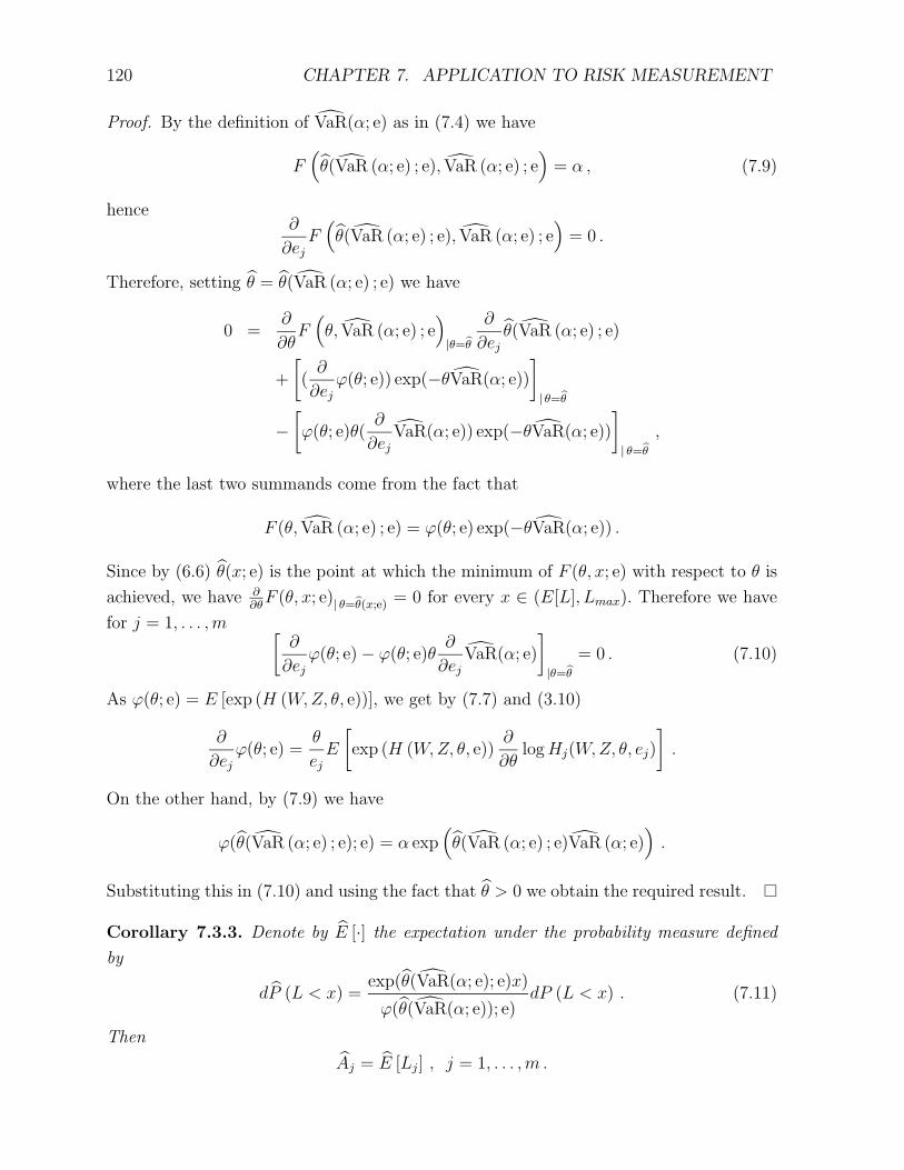
120 CHAPTER 7. APPLICATION TO RISK MEASUREMENT
Proof. By the definition of VaR(α; e) as in (7.4) we have
F(θ(VaR (α; e) ; e), VaR (α; e) ; e
)= α , (7.9)
hence∂
∂ejF(θ(VaR (α; e) ; e), VaR (α; e) ; e
)= 0 .
Therefore, setting θ = θ(VaR (α; e) ; e) we have
0 =∂
∂θF(θ, VaR (α; e) ; e
)|θ=θ
∂
∂ejθ(VaR (α; e) ; e)
+
[(∂
∂ejϕ(θ; e)) exp(−θVaR(α; e))
]| θ=θ
−[ϕ(θ; e)θ(
∂
∂ejVaR(α; e)) exp(−θVaR(α; e))
]| θ=θ
,
where the last two summands come from the fact that
F (θ, VaR (α; e) ; e) = ϕ(θ; e) exp(−θVaR(α; e)) .
Since by (6.6) θ(x; e) is the point at which the minimum of F (θ, x; e) with respect to θ is
achieved, we have ∂∂θF (θ, x; e)| θ=θ(x;e) = 0 for every x ∈ (E[L], Lmax). Therefore we have
for j = 1, . . . ,m [∂
∂ejϕ(θ; e)− ϕ(θ; e)θ
∂
∂ejVaR(α; e)
]|θ=θ
= 0 . (7.10)
As ϕ(θ; e) = E [exp (H (W,Z, θ, e))], we get by (7.7) and (3.10)
∂
∂ejϕ(θ; e) =
θ
ejE
[exp (H (W,Z, θ, e))
∂
∂θlogHj(W,Z, θ, ej)
].
On the other hand, by (7.9) we have
ϕ(θ(VaR (α; e) ; e); e) = α exp(θ(VaR (α; e) ; e)VaR (α; e)
).
Substituting this in (7.10) and using the fact that θ > 0 we obtain the required result.
Corollary 7.3.3. Denote by E [·] the expectation under the probability measure defined
by
dP (L < x) =exp(θ(VaR(α; e); e)x)
ϕ(θ(VaR(α; e)); e)dP (L < x) . (7.11)
Then
Aj = E [Lj] , j = 1, . . . ,m .
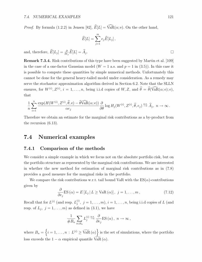
7.4. NUMERICAL EXAMPLES 121
Proof. By formula (1.2.2) in Jensen [82], E[L] = VaR(α; e). On the other hand,
E[L] =m∑j=1
ejE[Lj] ,
and, therefore, E[Lj] = ∂∂ejE[L] = Aj.
Remark 7.3.4. Risk contributions of this type have been suggested by Martin et al. [109]
in the case of a one-factor Gaussian model (W = 1 a.s. and p = 1 in (3.5)). In this case it
is possible to compute these quantities by simple numerical methods. Unfortunately this
cannot be done for the general heavy-tailed model under consideration. As a remedy may
serve the stochastoc approximation algorithm derived in Section 6.2. Note that the SLLN
ensures, for W (i), Z(i), i = 1, . . . , n, being i.i.d copies of W,Z, and θ = θ(VaR(α; e); e),
that
1
n
n∑i=1
exp(H(W (i), Z(i), θ, e)− θVaR(α; e))
αej
∂
∂θlogHj(W
(i), Z(i), θ, ej)a.s.→ Aj, n→∞ .
Therefore we obtain an estimate for the marginal risk contributions as a by-product from
the recursion (6.13).
7.4 Numerical examples
7.4.1 Comparison of the methods
We consider a simple example in which we focus not on the absolute portfolio risk, but on
the portfolio structure as represented by the marginal risk contributions. We are interested
in whether the new method for estimation of marginal risk contributions as in (7.8)
provides a good measure for the marginal risks in the portfolio.
We compare the risk contributions w.r.t. tail bound VaR with the ES(α)-contributions
given by∂
∂ejES (α) = E [Lj |L ≥ VaR (α)] , j = 1, . . . ,m , (7.12)
Recall that for L(i) (and resp. L(i)j , j = 1, . . . ,m), i = 1, . . . , n, being i.i.d copies of L (and
resp. of Lj, j = 1, . . . ,m) as defined in (3.1), we have
1
#Bn
∑i∈Bn
L(i)j
a.s.→ ∂
∂ejES (α) , n→∞ ,
where Bn =i = 1, . . . , n : L(i) ≥ VaR (α)
is the set of simulations, where the portfolio
loss exceeds the 1− α empirical quantile VaR (α).
122 CHAPTER 7. APPLICATION TO RISK MEASUREMENT
However, as #Bn increases slowly with the increase of n, extensive Monte Carlo sim-
ulation of all random components of L is necessary, see Overbeck [122], or Merino and
Nyfeler [114].
Example 7.4.1. [Portfolio with concentration in 1 credit]
The parameters of the considered model (as in (3.1) with (3.4) and (3.5)) are as follows:
0.0065 0.35
0.85
0.9
0.95
1
Exposure
Mar
gina
l con
tribu
tion
average ES contribution, small creditsES contribution, large creditUpper bound contribution, small creditsUpper bound contribution, large credit
0.0065 0.350.6
0.7
0.8
0.9
1
Exposure
Mar
gina
l con
tribu
tion
ES contributions, small creditsES contribution, large creditUpper bound contribution, small creditsUpper bound contribution, large credit
Figure 7.1: The parameters are the same as in Example 7.4.1.Left figure: the marginal risk contribution of the largest credit and the average marginal risk contributionof the small credits w.r.t the Expected Shortfall, as defined in (7.12), compared to the contributions w.r.tthe upper bound approximation, as defined in (7.8). The results are similar in terms of distance betweenthe small credits and the large one.Right figure: the marginal risk contributions w.r.t the two risk measures ES(α) and VaR(α). We used10 000 Monte Carlo simulations of all random components of L to compute the ES-contributions (7.12)and the same number of simulations of the common factors Z and global shock W to compute the upperbound contributions (7.8) as in Remark 7.3.4. Due to the error from the simulation, with the ES-method,equivalent credits have different contributions. The new upper bound method avoids this problem.
- m = 101 credits in the portfolio;
- exposures e1 = e2 = . . . = em−1 = 0.0065 and em = 0.35;
- rating system with K = 2 ratings (default and non-default);
- default probabilities P (Xj = 1) = pj,1 = 0.02, j = 1, . . . ,m;
- the marginal loss distributions are given as Lj = IXj=1, j = 1, . . . ,m.
For the dependence structure we use in (3.5) the t-model with ν = 4 degrees of freedom
and one common factor (p = 1) with factor loadings αj,1 = 0.8, j = 1, . . . ,m.
The parameters in this example are selected in such a way that the portfolio is com-
pletely homogeneous, except for one of the credits, whose exposure is very large. A rea-
sonable method for the computation of the marginal risk contributions should give equal
contributions for all credits except the largest, which obviously contributes much more to
the portfolio risk.
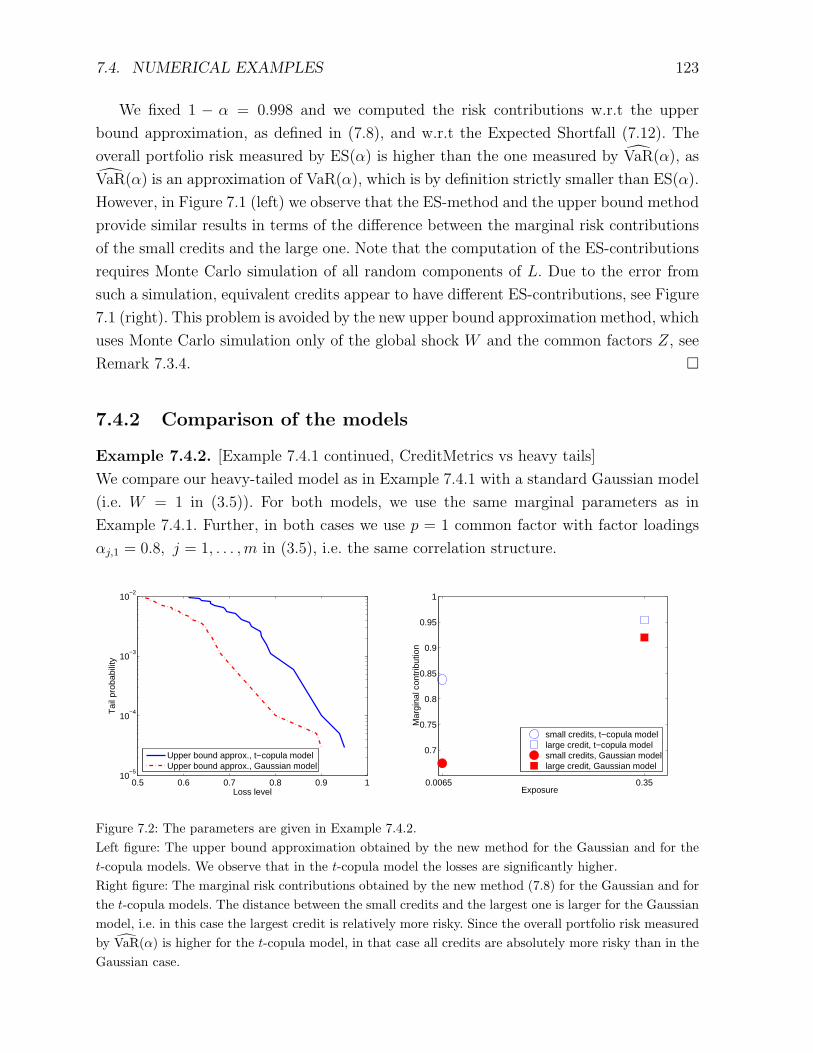
7.4. NUMERICAL EXAMPLES 123
We fixed 1 − α = 0.998 and we computed the risk contributions w.r.t the upper
bound approximation, as defined in (7.8), and w.r.t the Expected Shortfall (7.12). The
overall portfolio risk measured by ES(α) is higher than the one measured by VaR(α), as
VaR(α) is an approximation of VaR(α), which is by definition strictly smaller than ES(α).
However, in Figure 7.1 (left) we observe that the ES-method and the upper bound method
provide similar results in terms of the difference between the marginal risk contributions
of the small credits and the large one. Note that the computation of the ES-contributions
requires Monte Carlo simulation of all random components of L. Due to the error from
such a simulation, equivalent credits appear to have different ES-contributions, see Figure
7.1 (right). This problem is avoided by the new upper bound approximation method, which
uses Monte Carlo simulation only of the global shock W and the common factors Z, see
Remark 7.3.4.
7.4.2 Comparison of the models
Example 7.4.2. [Example 7.4.1 continued, CreditMetrics vs heavy tails]
We compare our heavy-tailed model as in Example 7.4.1 with a standard Gaussian model
(i.e. W = 1 in (3.5)). For both models, we use the same marginal parameters as in
Example 7.4.1. Further, in both cases we use p = 1 common factor with factor loadings
αj,1 = 0.8, j = 1, . . . ,m in (3.5), i.e. the same correlation structure.
0.5 0.6 0.7 0.8 0.9 110
−5
10−4
10−3
10−2
Loss level
Tai
l pro
babi
lity
Upper bound approx., t−copula modelUpper bound approx., Gaussian model
0.0065 0.35
0.7
0.75
0.8
0.85
0.9
0.95
1
Exposure
Mar
gina
l con
trib
utio
n
small credits, t−copula modellarge credit, t−copula modelsmall credits, Gaussian modellarge credit, Gaussian model
Figure 7.2: The parameters are given in Example 7.4.2.Left figure: The upper bound approximation obtained by the new method for the Gaussian and for thet-copula models. We observe that in the t-copula model the losses are significantly higher.Right figure: The marginal risk contributions obtained by the new method (7.8) for the Gaussian and forthe t-copula models. The distance between the small credits and the largest one is larger for the Gaussianmodel, i.e. in this case the largest credit is relatively more risky. Since the overall portfolio risk measuredby VaR(α) is higher for the t-copula model, in that case all credits are absolutely more risky than in theGaussian case.
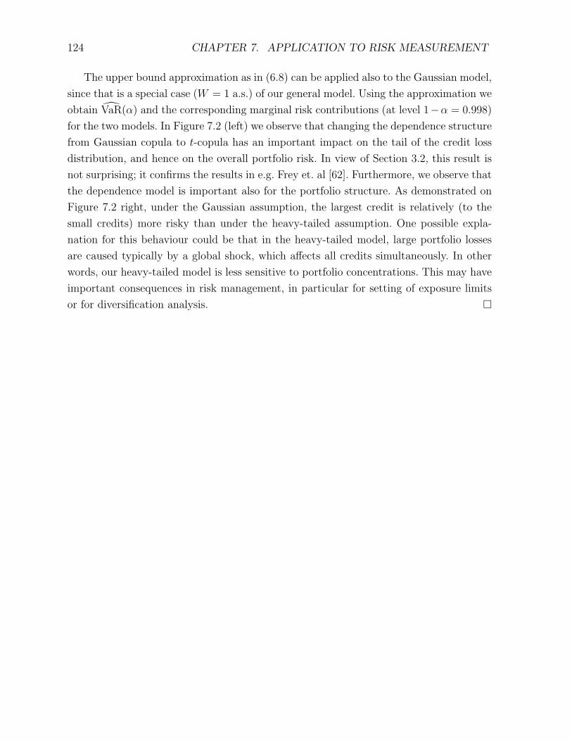
124 CHAPTER 7. APPLICATION TO RISK MEASUREMENT
The upper bound approximation as in (6.8) can be applied also to the Gaussian model,
since that is a special case (W = 1 a.s.) of our general model. Using the approximation we
obtain VaR(α) and the corresponding marginal risk contributions (at level 1−α = 0.998)
for the two models. In Figure 7.2 (left) we observe that changing the dependence structure
from Gaussian copula to t-copula has an important impact on the tail of the credit loss
distribution, and hence on the overall portfolio risk. In view of Section 3.2, this result is
not surprising; it confirms the results in e.g. Frey et. al [62]. Furthermore, we observe that
the dependence model is important also for the portfolio structure. As demonstrated on
Figure 7.2 right, under the Gaussian assumption, the largest credit is relatively (to the
small credits) more risky than under the heavy-tailed assumption. One possible expla-
nation for this behaviour could be that in the heavy-tailed model, large portfolio losses
are caused typically by a global shock, which affects all credits simultaneously. In other
words, our heavy-tailed model is less sensitive to portfolio concentrations. This may have
important consequences in risk management, in particular for setting of exposure limits
or for diversification analysis.
Chapter 8
Conclusions
In a global economy, it is no longer possible to explain the dependence between various
financial assets entirely by modelling their linear correlation. In this thesis, we analysed
a portfolio credit risk model with heavy-tailed risk factors to introduce non-linear (tail)
dependence.
First, we looked at the model’s input. With respect to the availability and the structure
of the input data, we made similar or even weaker assumptions than the assumptions in
the standard for the industry CreditMetrics model. We suggested new calibration methods
which make use of the information contained in the joint extreme observations. The
accuracy and the robustness of the estimators were investigated in simulations as well
as in several real-data studies.
Second, we looked at the model’s output. We developed (1) an importance sampling
algorithm and (2) a semi-analytic approximation for the tail of the portfolio loss distri-
bution. These methods allow, holding the computational time costs fixed, for tail and
quantile estimation of the portfolio loss and for narrow confidence bounds beyond the
range of the simulated by straightforward Monte Carlo methods scenarios. The tail ap-
proximation turned out to be quite useful in portfolio analysis, as it gives a by-product –
estimates of the contributions of the marginal credits to the overall portfolio risk.
Throughout the thesis we compared various aspects of the heavy-tailed and the Cred-
itMetrics model. We identified the key parameters which imply the difference in the tail
behaviour of the credit portfolio loss in the two models. Not only does a heavy-tailed
model lead to higher portfolio risk than the CreditMetrics model, and thus to e.g. higher
risk capital requirements. It changes significantly the risk structure within a credit port-
folio, and assuming it may lead to completely different results in an exposure or in a
diversification analysis.
125

126 CHAPTER 8. CONCLUSIONS

Bibliography
[1] Allen, L. and Saunders, A. (2002): Credit Risk Measurement. John Wiley & Sons,
Inc., New York.
[2] Altman, E. (1989): Measuring corporate bond mortality and performance. Journal
of Finance 9, 909-922.
[3] Altman, E. (1993): Defaulted bonds: demand, supply and performance 1987-1992.
Financial Analysts Journal 6, 55-60.
[4] Altman, E. and Kishore, V. (1996): Almost everything you wanted to know about
recoveries on defaulted bonds. Financial Analysts Journal 12, 57-64.
[5] Andersen, P., Borgan, O., Gill, R. and Keiding, N. (1993): Statistical Models for
Counting Processes. Springer, New York.
[6] Artzner, P., Delbaen, F., Eber, J.-M. and Heath, D. (1999): Coherent measures of
risk. Mathematical Finance 9, 203-228.
[7] Asmussen, S. (2000): Ruin Probabilities. World Scientific Piblishing, Singapore.
[8] Bank of International Settlements (1999): Credit risk modelling: current practices
and applications. Basel Committee on Banking Supervision, Basel.
[9] Bank of International Settlements (2001): The New Basel Capital Accord. Basel Com-
mittee on Banking Supervision, Basel.
[10] Basrak, B. (2000): The Sample Autocorrelation Function of Non-Linear Time Series.
Ph.D. thesis, Rijksuniversiteit Groningen.
Available at www.ub.rug.nl/eldoc/dis/science/b.basrak/.
[11] Becker, K., Isimbabi, M. Ogden, J. and Tucker, A. (1994): Contemporary Portfolio
Theory and Risk Management. West Publishing, Minneapolis.
[12] Behar, R. and Nagpal, K. (1999): Dynamics of rating migration. Working paper,
Standard & Poor’s. Available at www.standardandpoors.com.
127
128 BIBLIOGRAPHY
[13] Bielecki, T. and Rutkowski, M. (2001): Credit Risk: Modelling, Valuation and Hedg-
ing. Springer, Berlin.
[14] Bingham, N.H. Goldie, C.M. and Teugels, J.L. (1987): Regular Variation. Cambridge
University press, Cambridge.
[15] Bluhm, C. (2003): CDO Modeling: techniques, examples and applications. Reseacrh
paper, HypoVereinsbank Munich. Available at www.defaultrisk.com.
[16] Bluhm, C., Overbeck, L. and Wagner, C. (2003): An Introduction to Credit Risk
Modeling. Chapman & Hall / CRC, Boca Raton.
[17] Breiman, L. (1965): On some limit theorems similar to the arc sin law. Theory Probab.
Appl. 10, 323-331.
[18] Bunning, H. and Trenkel, G. (1978): Non-parametric Statistical Methods. Walter de
Gruyter Verlag, Berlin.
[19] Cantor, R. and Hamilton, D. (2004): Rating migrations and defaults conditional on
watchlist, outlook and rating history. Special comment, Moody’s Investment Service.
Available at www.moodys.com.
[20] Carty, L. and Fons, J. (1994): Measuring changes in corporate credit quality. The
Journal of Fixed Income 6, 66-78.
[21] Casella, L. and Berger, R. (2002): Statistical Inference. Duxbury Press Pacific Grove,
London.
[22] Coles, S., Heffernan, J. and Tawn, J. (1999): Dependence Measures for Extreme Value
Analyses. Extremes 2, 339-365.
[23] Collett, D. (1999): Modelling Binary Data. Chapman & Hall, London.
[24] Cont, R. (2001): Empirical properties of asset returns. Stylized facts and statistical
issues. Quantitative Finance 1, 223-236.
[25] Credit Suiss Financial Products (1997): CreditRisk+ - a Credit Risk Management
Framework.
[26] Czado, C. (2000): Multivariate regression analysis of panel aata with binary outcomes
applied to unemployment data. Statistical Papers 41, 281-304.
[27] Das, S., and Geng, G. (2002): Modeling the processes of correlated default. Working
paper, Santa Clara University. Available at www.defaultrisk.com.
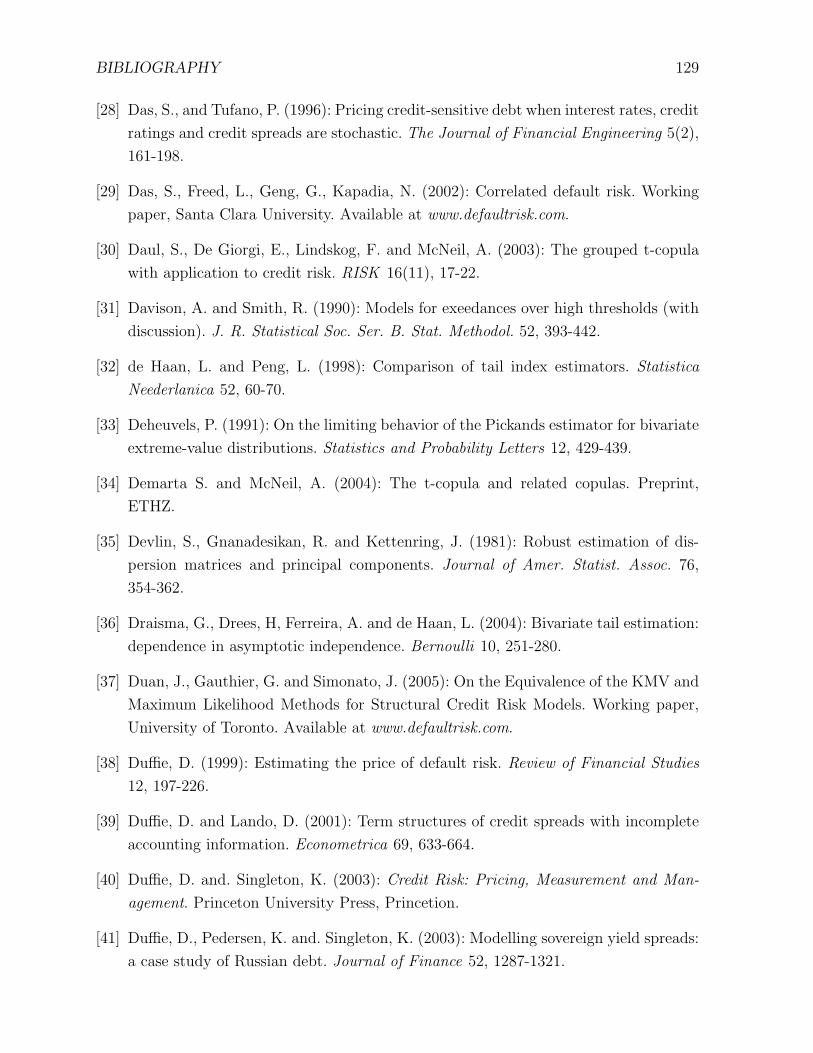
BIBLIOGRAPHY 129
[28] Das, S., and Tufano, P. (1996): Pricing credit-sensitive debt when interest rates, credit
ratings and credit spreads are stochastic. The Journal of Financial Engineering 5(2),
161-198.
[29] Das, S., Freed, L., Geng, G., Kapadia, N. (2002): Correlated default risk. Working
paper, Santa Clara University. Available at www.defaultrisk.com.
[30] Daul, S., De Giorgi, E., Lindskog, F. and McNeil, A. (2003): The grouped t-copula
with application to credit risk. RISK 16(11), 17-22.
[31] Davison, A. and Smith, R. (1990): Models for exeedances over high thresholds (with
discussion). J. R. Statistical Soc. Ser. B. Stat. Methodol. 52, 393-442.
[32] de Haan, L. and Peng, L. (1998): Comparison of tail index estimators. Statistica
Neederlanica 52, 60-70.
[33] Deheuvels, P. (1991): On the limiting behavior of the Pickands estimator for bivariate
extreme-value distributions. Statistics and Probability Letters 12, 429-439.
[34] Demarta S. and McNeil, A. (2004): The t-copula and related copulas. Preprint,
ETHZ.
[35] Devlin, S., Gnanadesikan, R. and Kettenring, J. (1981): Robust estimation of dis-
persion matrices and principal components. Journal of Amer. Statist. Assoc. 76,
354-362.
[36] Draisma, G., Drees, H, Ferreira, A. and de Haan, L. (2004): Bivariate tail estimation:
dependence in asymptotic independence. Bernoulli 10, 251-280.
[37] Duan, J., Gauthier, G. and Simonato, J. (2005): On the Equivalence of the KMV and
Maximum Likelihood Methods for Structural Credit Risk Models. Working paper,
University of Toronto. Available at www.defaultrisk.com.
[38] Duffie, D. (1999): Estimating the price of default risk. Review of Financial Studies
12, 197-226.
[39] Duffie, D. and Lando, D. (2001): Term structures of credit spreads with incomplete
accounting information. Econometrica 69, 633-664.
[40] Duffie, D. and. Singleton, K. (2003): Credit Risk: Pricing, Measurement and Man-
agement. Princeton University Press, Princetion.
[41] Duffie, D., Pedersen, K. and. Singleton, K. (2003): Modelling sovereign yield spreads:
a case study of Russian debt. Journal of Finance 52, 1287-1321.
130 BIBLIOGRAPHY
[42] Duhamel, P. and Vetterli, M. (1990): Fast Fourier transforms: a tutorial review and
a state of the art. Signal Processing 19, 259-299.
[43] Dupois, P. and Ellis, R. (1997): A Weak Convergence Approach to the Theory of
Large Deviations. Wiley, New York.
[44] Eberhart, A. and Sweeny, R. (1992): Does the bond market predict bankupcy settle-
ments? Journal of Finance 3, 943-980.
[45] Embrechts, P., Hoeing, A. and Juri, A. (2003): Using Copulae to bound the Value-
at-Risk for functions of dependent risks. Finance and Stochastics 7(2), 145-167.
[46] Embrechts, P., Kluppelberg, C. and Mikosch, T. (1997): Modelling Extremal Events
for Insurance and Finance. Springer, Berlin.
[47] Embrechts, P., Lindskog, F. and McNeil, A. (2001): Modelling dependence with copu-
las and applications to risk management. In: Handbook of Heavy Tailed Distributions
in Finance, 329-384, ed. S. Rachev, Elsevier.
[48] Embrechts, P., McNeil, A. and Straumann, D. (1999): Correlation and dependence
in risk management: properties and pitfalls. In: Risk Management: VaR and beyond,
Cambridge University press, Cambridge.
[49] Emmer, S. and Kluppelberg (1998): VaR - a measure for extreme risks. Solutions 2,
53-56.
[50] Fang, K.T., Kotz, S. and Ng, K.W. (1990): Symmetric Multivariate and Related
Distributions. Chapman & Hall, London.
[51] Finger, C. (1998): Credit derivatives in CreditMetrics. CreditMetrics Monitor 3.
[52] Finger, C. (1999): Conditional approaches for CreditMetrics portfolio distribution.
CreditMetrics Monitor 1.
[53] Finger, C. (1999): Risk-return reporting. CreditMetrics Monitor 1.
[54] Fishburn, P.C. (1977): Mean-risk analysis with risk associated with below-target
returns. American Economic Review 67, 116-126.
[55] Follmer, H. and Leukert, P. (1999): Quantile hedging. Finance and Stochastics 3,
251-273.
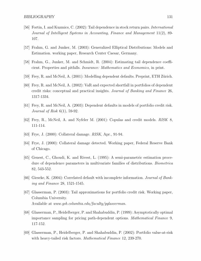
BIBLIOGRAPHY 131
[56] Fortin, I. and Kuzmics, C. (2002): Tail dependence in stock return pairs. International
Journal of Intelligent Systems in Accounting, Finance and Management 11(2), 89-
107.
[57] Frahm, G. and Junker, M. (2003): Generalized Elliptical Distributions: Models and
Estimation. working paper, Research Center Caesar, Germany.
[58] Frahm, G., Junker, M. and Schmidt, R. (2004): Estimating tail dependence coeffi-
cient. Properties and pitfalls. Insurance: Mathematics and Economics, in print.
[59] Frey, R. and McNeil, A. (2001): Modelling dependent defaults. Preprint, ETH Zurich.
[60] Frey, R. and McNeil, A. (2002): VaR and expected shortfall in portfolios of dependent
credit risks: conceptual and practical insights. Journal of Banking and Finance 26,
1317-1334.
[61] Frey, R. and McNeil, A. (2003): Dependent defaults in models of portfolio credit risk.
Journal of Risk 6(1), 59-92.
[62] Frey, R., McNeil, A. and Nyfeler M. (2001): Copulas and credit models. RISK 8,
111-114.
[63] Frye, J. (2000): Collateral damage. RISK, Apr., 91-94.
[64] Frye, J. (2000): Collateral damage detected. Working paper, Federal Reserve Bank
of Chicago.
[65] Genest, C., Ghoudi, K. and Rivest, L. (1995): A semi-parametric estimation proce-
dure of dependence parameters in multivariate families of distributions. Biometrica
82, 543-552.
[66] Gieseke, K. (2004): Correlated default with incomplete information. Journal of Bank-
ing and Finance 28, 1521-1545.
[67] Glasserman, P. (2003): Tail approximations for portfolio credit risk. Working paper,
Columbia University.
Available at www.gsb.columbia.edu/faculty/pglasserman.
[68] Glasserman, P., Heidelberger, P. and Shahabuddin, P. (1999): Asymptotically optimal
importance sampling for pricing path-dependent options. Mathematical Finance 9,
117-152.
[69] Glasserman, P., Heidelberger, P. and Shahabuddin, P. (2002): Portfolio value-at-risk
with heavy-tailed risk factors. Mathematical Finance 12, 239-270.
132 BIBLIOGRAPHY
[70] Glasserman, P. and Li, J. (2004): Importance sampling for portfolio credit risk. Work-
ing paper, Columbia University.
Available at www.gsb.columbia.edu/faculty/pglasserman.
[71] Gordy, M. (2000): A comparative anatomy of credit risk models. Journal of Banking
and Finance 24, 119-149.
[72] Gordy, M. (2001): A risk factor model foundation for rating-based bank capital rules.
Journal of Financial Intermediation 12, 199-232.
[73] Gordy, M. (2002): Saddlepoint approximation of CreditRisk+. Journal of Banking
and Finance 26, 1335-1353.
[74] Gupton, G., Bhatia, M. and Finger, C. (1997): CreditMetrics – Technical document.
J.P.Morgan, New York.
[75] Gupton, G. and Stein, R. (2005): LossCalc v2: Dynamic prediction of LGD. Research
paper, KMV. Available at www.defaultrisk.com.
[76] Hamilton, D., Gupton, G. and Berthault, A. (2001): Default and recovery rates of cor-
porate bond issuers: 2000. Special comment, Moody’s Investment Service. Available
at www.moodys.com.
[77] Hoffding, W. (1947): On the distribution of the rank correlation coefficient τ whern
the variates are not independent. Biometrica 34, 183-196.
[78] Hult, H. and Lindskog, F. (2001): Multivariate extremes, aggregation and dependence
in elliptical distributions. Advances in Applied Probability 34(3), 587-608.
[79] Israel, R., Rosenthal, J. and Wei, J. (2001): Finding generators for Markov chains
via empirical transition matrices, with applications to credit ratings. Mathematical
Finance, 11(2), 245-265.
[80] Jarrow, R. and Turnbull, S. (1995): Pricing derivatives on financial securities subject
to credit risk. Journal of Finance 50, 53-85.
[81] Jarrow, R., Lando, D. and Turnbull, S. (1997): A Markov model for the term structure
of credit risk spreads. Review of Financial Studies 10, 481-523.
[82] Jensen, J. (1995): Saddlepoint Approximations. Oxford University press, Oxford.
[83] Joe, H. (1997): Multivariate Models and Dependence Concepts. Chapman & Hall,
New York.
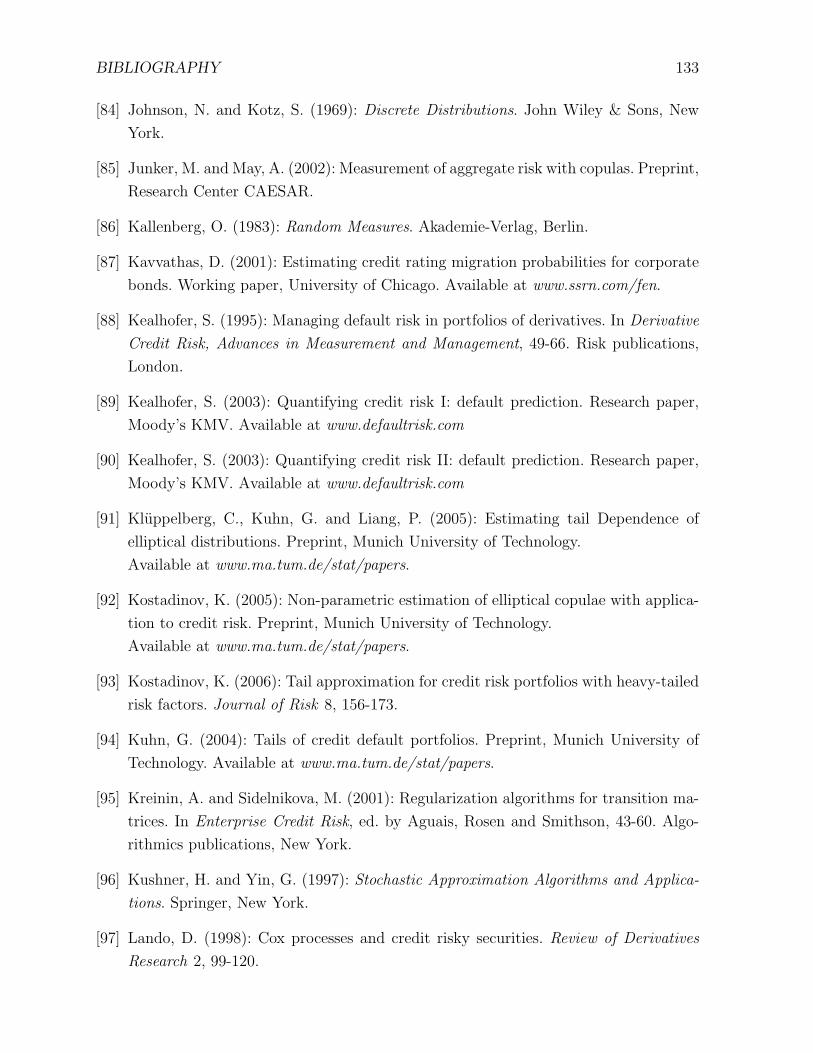
BIBLIOGRAPHY 133
[84] Johnson, N. and Kotz, S. (1969): Discrete Distributions. John Wiley & Sons, New
York.
[85] Junker, M. and May, A. (2002): Measurement of aggregate risk with copulas. Preprint,
Research Center CAESAR.
[86] Kallenberg, O. (1983): Random Measures. Akademie-Verlag, Berlin.
[87] Kavvathas, D. (2001): Estimating credit rating migration probabilities for corporate
bonds. Working paper, University of Chicago. Available at www.ssrn.com/fen.
[88] Kealhofer, S. (1995): Managing default risk in portfolios of derivatives. In Derivative
Credit Risk, Advances in Measurement and Management, 49-66. Risk publications,
London.
[89] Kealhofer, S. (2003): Quantifying credit risk I: default prediction. Research paper,
Moody’s KMV. Available at www.defaultrisk.com
[90] Kealhofer, S. (2003): Quantifying credit risk II: default prediction. Research paper,
Moody’s KMV. Available at www.defaultrisk.com
[91] Kluppelberg, C., Kuhn, G. and Liang, P. (2005): Estimating tail Dependence of
elliptical distributions. Preprint, Munich University of Technology.
Available at www.ma.tum.de/stat/papers.
[92] Kostadinov, K. (2005): Non-parametric estimation of elliptical copulae with applica-
tion to credit risk. Preprint, Munich University of Technology.
Available at www.ma.tum.de/stat/papers.
[93] Kostadinov, K. (2006): Tail approximation for credit risk portfolios with heavy-tailed
risk factors. Journal of Risk 8, 156-173.
[94] Kuhn, G. (2004): Tails of credit default portfolios. Preprint, Munich University of
Technology. Available at www.ma.tum.de/stat/papers.
[95] Kreinin, A. and Sidelnikova, M. (2001): Regularization algorithms for transition ma-
trices. In Enterprise Credit Risk, ed. by Aguais, Rosen and Smithson, 43-60. Algo-
rithmics publications, New York.
[96] Kushner, H. and Yin, G. (1997): Stochastic Approximation Algorithms and Applica-
tions. Springer, New York.
[97] Lando, D. (1998): Cox processes and credit risky securities. Review of Derivatives
Research 2, 99-120.
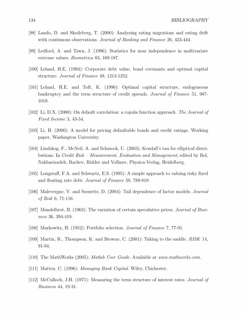
134 BIBLIOGRAPHY
[98] Lando, D. and Skodeberg, T. (2000): Analyzing rating migrations and rating drift
with continuous observations. Journal of Banking and Finance 26, 423-444.
[99] Ledford, A. and Tawn, J. (1996): Statistics for near independence in multivariate
extreme values. Biometrica 83, 169-187.
[100] Leland, H.E. (1994): Corporate debt value, bond covenants and optimal capital
structure. Journal of Finance 49, 1213-1252.
[101] Leland, H.E. and Toft, K. (1996): Optimal capital structure, endogeneous
bankruptcy and the term structure of credit spreads. Journal of Finance 51, 987-
1019.
[102] Li, D.X. (2000): On default correlation: a copula function approach. The Journal of
Fixed Income 3, 43-54.
[103] Li, H. (2000): A model for pricing defaultable bonds and credit ratings. Working
paper, Washington University.
[104] Lindskog, F., McNeil, A. and Schmock, U. (2003): Kendall’s tau for elliptical distri-
butions. In Credit Risk – Measurement, Evaluation and Management, edited by Bol,
Nakhaeizadeh, Rachev, Ridder and Vollmer, Physica-Verlag, Heidelberg.
[105] Longstaff, F.A. and Schwartz, E.S. (1995): A simple approach to valuing risky fixed
and floating rate debt. Journal of Finance 50, 789-819.
[106] Malevergne, Y. and Sornette, D. (2004): Tail dependence of factor models. Journal
of Risk 6, 71-116.
[107] Mandelbrot, B. (1963): The variation of certain speculative prices. Journal of Busi-
ness 36, 394-419.
[108] Markowitz, H. (1952): Portfolio selection. Journal of Finance 7, 77-91.
[109] Martin, R., Thompson, K. and Browne, C. (2001): Taking to the saddle. RISK 14,
91-94.
[110] The MathWorks (2005): Matlab User Guide. Available at www.mathworks.com.
[111] Matten. C. (1996): Managing Bank Capital. Wiley, Chichester.
[112] McCulloch, J.H. (1971): Measuring the term structure of interest rates. Journal of
Business 44, 19-31.
BIBLIOGRAPHY 135
[113] Mcleish, D. and Small, C. (1988): The Theory and Applications of Statistical Infer-
ence Functions, vol. 44 of Lecture Notes in Statistics, Springer, New York.
[114] Merino, S. and Nyfeler, M. (2004): Applying importance sampling for estimating
coherent risk contributions. Quantitative Finance 4, 199-207.
[115] Merton, R (1974): On the pricing of corporate debt. Journal of Finance 29, 449-470.
[116] Mikosch, T. (2001): Modelling dependence and tails of financial time series. In Sem-
Stat: Seminaire Europeen de Statistique, Extreme Value Theory and Applications, ed.
by H. Rootzen and B. Finkenstadt, Chapman and Hall, London.
[117] Mina, J. and Ulmer, A. (1999): Delta-gamma four ways. Working paper, RiskMetrics
group. Available at www.riskmetrics.com.
[118] Nelsen, R. (1999): An Introduction to Copulas. Springer, New York.
[119] Nelson, R. and Siegel, A. (1987): Parsimonious modelling of yield curves. Journal
of Business 60, 473-499.
[120] Nickell, P., Perraudin, W. and Varotto, S. (2000): Stability of rating migrations.
Journal of Banking and Finance 24, 203-228.
[121] Oda, N. and Muranaga, J. (1997): A new framework for measuring credit risk of a
portfolio: The ’ExVaR’ model. Monetary and Economic Studies 15, Bank of Japan.
[122] Overbeck, L. (2000): Allocation of economic capital in loan portfolios. In Proceedings
’Measuring Risk In Complex Stochastic Systems’, Springer, Berlin.
[123] Petrov, V. (1995): Limit Theorems of Probability Theory. Oxford Univ. Press, New
York.
[124] Resnick, S.I, (1987): Extreme Values, Regular Variation and Point Processes.
Springer, New York.
[125] Rousseeuw, P. and Molenberghs, G. (1993): Transformations of non positive semidef-
inite correlation matrices. Comm. Statist. A – Theory and Methods 4, 965-984.
[126] Schmidt, R. (2002): Tail dependence for elliptically contoured distributions. Math-
ematical Methods of Operations Research 55, 301-327.
[127] Schmidt, R. and Stadtmuller, U. (2003): Non-parametric estimation of tail depen-
dence. Scandinavian Journal of Statistics, in print.
136 BIBLIOGRAPHY
[128] Schlather, M. and Tawn, J.A. (2003): A dependence measure for multivariate and
spatial extreme values: properties and inference. Biometrica 90 (1), 139-156.
[129] Schonbucher, P. (2003): Credit Derivatives Pricing Models. John Wiley & Sons,
Chichester, England.
[130] Schonbucher, P. and Schubert, D. (2001): Copula dependent default risk in intensity
models. Working paper, Bonn University.
[131] Schwarz, C. (2005): Eine gruppierte elliptische Copula und ihre Anwendung im
Kreditrisikomanagement. Diploma thesis, Munich University of Technology.
[132] Smith, R.L (1987): Estimating tails of probability distributions. Annals of Statistics
15, 1174-1207.
[133] Sklar, A. (1996): Random variables, distribution functions, and copulas – a personal
look backward and forward. In Distributions with Fixed Marginals and Related Topics
1-14, ed. by L. Ruschendorff, B. Schweizer and M. Taylor, Institute of Mathematical
Statistics, Hayward, CA.
[134] Tasche, D. (2000): Risk contributions and performance measurement. Working pa-
per, TU Munchen. Available at www.ma.tum.de/stat.
[135] Wendin, J. (2002): Estimation of the Spectral Measure and the Tail Dependence Co-
efficient for Regularly Varying Random Vectors. Ph.D. thesis, ETH Zurich. Available
at www.math.ethz.ch/ wendin.
[136] Zhou, C. (1997): A jump-diffusion approach to modelling credit risk and valuing
defaultable secuities. Discussion paper, Board of Governors of the Federal Reserve
System. Available at www.defaultrisk.com.


