Embed Size (px)
Citation preview

Alma Mater Studiorum — Universita di Bologna
DOTTORATO DI RICERCA IN INFORMATICA
Ciclo: XXVII
Settore Concorsuale di afferenza: 01/B1
Settore Scientifico disciplinare: INF/01
Portfolio Approaches inConstraint Programming
Candidato: Roberto Amadini
Coordinatore Dottorato: Relatore:
Maurizio Gabbrielli Maurizio Gabbrielli
Esame finale anno 2015


Abstract
Recent research has shown that the performance of a single, arbitrarily efficient
algorithm can be significantly outperformed by using a portfolio of —possibly on-
average slower— algorithms. Within the Constraint Programming (CP) context, a
portfolio solver can be seen as a particular constraint solver that exploits the synergy
between the constituent solvers of its portfolio for predicting which is (or which are)
the best solver(s) to run for solving a new, unseen instance.
In this thesis we examine the benefits of portfolio solvers in CP. Despite portfolio
approaches have been extensively studied for Boolean Satisfiability (SAT) problems,
in the more general CP field these techniques have been only marginally studied
and used. We conducted this work through the investigation, the analysis and
the construction of several portfolio approaches for solving both satisfaction and
optimization problems. We focused in particular on sequential approaches, i.e.,
single-threaded portfolio solvers always running on the same core.
We started from a first empirical evaluation on portfolio approaches for solving
Constraint Satisfaction Problems (CSPs), and then we improved on it by introduc-
ing new data, solvers, features, algorithms, and tools. Afterwards, we addressed
the more general Constraint Optimization Problems (COPs) by implementing and
testing a number of models for dealing with COP portfolio solvers. Finally, we have
come full circle by developing sunny-cp: a sequential CP portfolio solver that turned
out to be competitive also in the MiniZinc Challenge, the reference competition for
CP solvers.
iii

iv
Acknowledgements
“Gratus animus est una virtus non solum maxima,
sed etiam mater virtutum omnium reliquarum”1
Marcus Tullius Cicero.
Writing acknowledgements is more difficult than it looks. There is always some-
one that you forget to mention, and probably those people will be among the few
that will read the acknowledgements. It is not just a selection task, but also a
scheduling problem: you do not have to only choose the people to thank, but even
who thank first and who later.
Let us begin by winding the timeline back about three years ago. If I have could
join the Ph.D. program, part of the credit can be taken by Prof. Gianfranco Rossi
—who introduced me to Constraint (Logic) Programming and also supervised my
Bachelor and Master theses— and Prof. Roberto Bagnara, both professors at the
University of Parma, which wrote the reference letters needed for the application.
Once I started the Ph.D. program, I had the opportunity to know friendly and
easygoing colleagues with whom I shared the moments of hopelessness and satis-
faction typical of every Ph.D. student. Among them, I would like in particular
to mention: Gioele Barabucci, Luca Bedogni, Flavio Bertini, Luca Calderoni, Or-
nela Dardha, Angelo Di Iorio, Jacopo Mauro, Andrea Nuzzolese, Giulio Pellitta,
1 “Gratitude is not only the greatest of virtues, but the parent of all others”.
v

Silvio Peroni, Francesco Poggi, Giuseppe Profiti, Alessandro Rioli, Imane Sefrioui,
Francesco Strappaveccia.
Almost all the work described in this thesis has been conducted together with
Prof. Maurizio Gabbrielli, the Ph.D. program coordinator as well as my supervisor,
and with Dr. Jacopo Mauro.
Let me say that it is not uncommon to hear about Ph.D. students treated as
employees, if not servants, by their supervisors. On the contrary, Maurizio is a very
good man and has been for me an ideal supervisor: he never put pressure on me,
leaving me almost total freedom of research.
Jacopo introduced me to Algorithm Portfolios, and has been the colleague that
most helped me during the doctorate course. We had sometimes lively debates, but
without his help it would have been very difficult to get the appreciable results we
achieved during these years.
During my Ph.D. program I also had a really enjoyable staying at the NICTA
(National ICT of Australia) Optimisation Research Group of Melbourne. In this
regard I would like to thank all the members of the group, and in particular: Dr.
Andreas Schutt, who helped me on some technical issues and also reviewed this
thesis; Prof. Peter J. Stuckey, my supervisor overseas, who gave me valuable and
interesting insights, and Alessandra Stasi, the group coordinator, for her precious
help on logistics and bureaucracy.
My sincere thanks to the reviewers of this thesis, Dr. Andreas Schutt and Prof.
Eric Monfroy, for their detailed and in-depth reviews and for their useful and infor-
mative comments.
I can say that these three years have been for me a positive turning point, not
only from the academic point of view. Many thanks to those who helped me to
achieve this goal, with apologies to those I have not mentioned above.
vi

Grazie
Il dottorato di ricerca e il massimo grado di istruzione universitaria ottenibile. Si
tratta senza ombra di dubbio di un traguardo significativo, una pietra miliare nel
percorso di crescita —non solo professionale— di una persona. Al di la dei dovuti
ringraziamenti di rito, il mio grazie piu grande va a coloro che piu di tutti hanno
contribuito al raggiungimento di questo titolo. Parlo ovviamente dei miei genitori,
Bruno e Tiziana.
vii

viii

Contents
Abstract iii
Acknowledgements v
1 Introduction 1
1.1 Outline . . . . . . . . . . . . . . . . . . . . . . . . . . . . . . . . . . . 3
2 Constraint Programming 7
2.1 Constraint Satisfaction Problems . . . . . . . . . . . . . . . . . . . . 8
2.1.1 CSP on Finite Domains . . . . . . . . . . . . . . . . . . . . . 11
2.1.1.1 Boolean Variables . . . . . . . . . . . . . . . . . . . 11
2.1.1.2 Integer Variables . . . . . . . . . . . . . . . . . . . . 13
2.1.1.3 Other Variables . . . . . . . . . . . . . . . . . . . . . 14
2.1.2 CSP Solving . . . . . . . . . . . . . . . . . . . . . . . . . . . . 15
2.1.2.1 Consistency techniques . . . . . . . . . . . . . . . . . 16
2.1.2.2 Propagation and Search . . . . . . . . . . . . . . . . 17
2.1.2.3 Nogood Learning and Lazy Clause Generation . . . . 18
2.1.2.4 Local Search . . . . . . . . . . . . . . . . . . . . . . 19
2.2 Constraint Optimization Problems . . . . . . . . . . . . . . . . . . . 20
2.2.1 Soft Constraints . . . . . . . . . . . . . . . . . . . . . . . . . . 21
2.2.1.1 Fuzzy Constraints and Weighted CSPs . . . . . . . . 22
ix

2.2.1.2 Formalism and Inference . . . . . . . . . . . . . . . . 22
2.2.2 Optimization and Operations Research . . . . . . . . . . . . . 23
2.2.2.1 Linear Programming . . . . . . . . . . . . . . . . . . 24
2.2.2.2 Nonlinear Programming . . . . . . . . . . . . . . . . 25
3 Portfolios of Constraint Solvers 29
3.1 Dataset . . . . . . . . . . . . . . . . . . . . . . . . . . . . . . . . . . 31
3.2 Solvers . . . . . . . . . . . . . . . . . . . . . . . . . . . . . . . . . . . 33
3.3 Features . . . . . . . . . . . . . . . . . . . . . . . . . . . . . . . . . . 34
3.4 Selectors . . . . . . . . . . . . . . . . . . . . . . . . . . . . . . . . . . 36
3.5 Related Work . . . . . . . . . . . . . . . . . . . . . . . . . . . . . . . 38
4 Portfolios of CSP Solvers 41
4.1 A First Empirical Evaluation . . . . . . . . . . . . . . . . . . . . . . 42
4.1.1 Methodology . . . . . . . . . . . . . . . . . . . . . . . . . . . 43
4.1.1.1 Dataset . . . . . . . . . . . . . . . . . . . . . . . . . 43
4.1.1.2 Solvers . . . . . . . . . . . . . . . . . . . . . . . . . . 44
4.1.1.3 Features . . . . . . . . . . . . . . . . . . . . . . . . . 45
4.1.1.4 Validation . . . . . . . . . . . . . . . . . . . . . . . . 46
4.1.1.5 Portfolios composition . . . . . . . . . . . . . . . . . 49
4.1.1.6 Off-the-shelf approaches . . . . . . . . . . . . . . . . 49
4.1.1.7 Other approaches . . . . . . . . . . . . . . . . . . . . 51
4.1.2 Results . . . . . . . . . . . . . . . . . . . . . . . . . . . . . . . 54
4.1.2.1 Percentage of Solved Instances . . . . . . . . . . . . 54
4.1.2.2 Average Solving Time . . . . . . . . . . . . . . . . . 58
4.1.2.3 Summary . . . . . . . . . . . . . . . . . . . . . . . . 59
4.2 An Enhanced Evaluation . . . . . . . . . . . . . . . . . . . . . . . . . 60
4.2.1 SUNNY: a Lazy Portfolio Approach . . . . . . . . . . . . . . . 61
4.2.1.1 SUNNY Algorithm . . . . . . . . . . . . . . . . . . . 62
x
4.2.2 Methodology . . . . . . . . . . . . . . . . . . . . . . . . . . . 67
4.2.2.1 Dataset . . . . . . . . . . . . . . . . . . . . . . . . . 67
4.2.2.2 Solvers . . . . . . . . . . . . . . . . . . . . . . . . . . 68
4.2.2.3 Features . . . . . . . . . . . . . . . . . . . . . . . . . 70
4.2.3 Results . . . . . . . . . . . . . . . . . . . . . . . . . . . . . . . 73
4.2.3.1 Percentage of Solved Instances . . . . . . . . . . . . 74
4.2.3.2 Average Solving Time . . . . . . . . . . . . . . . . . 75
4.2.3.3 sunny-csp . . . . . . . . . . . . . . . . . . . . . . . 77
4.2.3.4 Training Cost . . . . . . . . . . . . . . . . . . . . . . 80
4.2.3.5 Summary . . . . . . . . . . . . . . . . . . . . . . . . 82
5 Portfolios of COP Solvers 85
5.1 An Empirical Evaluation of COP Portfolio Approaches . . . . . . . . 86
5.1.1 Evaluating COP solvers . . . . . . . . . . . . . . . . . . . . . 87
5.1.1.1 The score function . . . . . . . . . . . . . . . . . . . 89
5.1.2 Methodology . . . . . . . . . . . . . . . . . . . . . . . . . . . 92
5.1.2.1 Solvers, Dataset, and Features . . . . . . . . . . . . . 92
5.1.2.2 Portfolio Approaches . . . . . . . . . . . . . . . . . . 93
5.1.3 Results . . . . . . . . . . . . . . . . . . . . . . . . . . . . . . . 96
5.1.3.1 Score . . . . . . . . . . . . . . . . . . . . . . . . . . 97
5.1.3.2 Optima Proven . . . . . . . . . . . . . . . . . . . . . 100
5.1.3.3 Optimization Time . . . . . . . . . . . . . . . . . . . 101
5.1.3.4 MiniZinc Challenge Score . . . . . . . . . . . . . . . 102
5.1.3.5 Summary . . . . . . . . . . . . . . . . . . . . . . . . 104
5.2 Sequential Time Splitting and Bound Communication . . . . . . . . . 105
5.2.1 Solving Behaviour and Timesplit Solvers . . . . . . . . . . . . 105
5.2.2 Splitting Selection and Evaluation . . . . . . . . . . . . . . . . 108
5.2.2.1 Evaluation Metrics . . . . . . . . . . . . . . . . . . . 109
xi

5.2.2.2 TimeSplit Algorithm . . . . . . . . . . . . . . . . . 112
5.2.2.3 TimeSplit Evaluation . . . . . . . . . . . . . . . . . 114
5.2.3 Timesplit Portfolio Solvers . . . . . . . . . . . . . . . . . . . . 116
5.2.3.1 Static Splitting . . . . . . . . . . . . . . . . . . . . . 118
5.2.3.2 Dynamic Splitting . . . . . . . . . . . . . . . . . . . 120
5.2.4 Empirical Evaluation . . . . . . . . . . . . . . . . . . . . . . . 120
5.2.4.1 Test Results . . . . . . . . . . . . . . . . . . . . . . . 123
5.2.4.2 Summary . . . . . . . . . . . . . . . . . . . . . . . . 126
6 sunny-cp: a CP Portfolio Solver 129
6.1 Architecture . . . . . . . . . . . . . . . . . . . . . . . . . . . . . . . . 130
6.1.1 Usage . . . . . . . . . . . . . . . . . . . . . . . . . . . . . . . 133
6.2 Validation . . . . . . . . . . . . . . . . . . . . . . . . . . . . . . . . . 136
6.3 Summary . . . . . . . . . . . . . . . . . . . . . . . . . . . . . . . . . 142
7 Conclusions and Extensions 145
References 149
xii

Chapter 1
Introduction
“Dimidium facti, qui coepit, habet”1
Quintus Horatius Flaccus.
The Constraint Programming (CP) paradigm is a general and powerful frame-
work that enables to express relations between different entities in form of con-
straints that must be satisfied. The concept of constraint is ubiquitous and not
confined to the sciences: constraints appear in every aspect of daily life in the form
of requirements, obligations, or prohibitions. For example, logistic problems like
task scheduling or resource allocation can be addressed by CP in a natural and el-
egant way. The CP paradigm, characterized as a sub-area of Artificial Intelligence,
is essentially based on two vertical layers:
(i) a modelling level, in which a real-life problem is identified, examined, and
formalized into a mathematical model by human experts;
(ii) a solving level, aimed at resolving as efficiently and comprehensively as possible
the model defined in (i) by means of software agents called constraint solvers.
1 “Well begun is half done”.
2 Chapter 1. Introduction
The goal of CP is to model and solve Constraint Satisfaction Problems (CSPs) as
well as Constraint Optimization Problems (COPs) [159]. Solving a CSP means to
find a solution that satisfies all the constraints of the problem. A COP is instead
a generalized CSP where we are also interested in optimal solutions, i.e., solutions
that minimize a cost or maximize a payoff.
The Algorithm Selection (AS) problem, for the first time formalized by John R.
Rice in 1976 [157], can be roughly reduced to the following question:
Given an input problem P and a set A = {A1, A2, . . . , An} of algorithms,
which is the “best” algorithm Ai ∈ A for solving problem P?
The underlying idea behind AS is very general and implicitly used in practical ev-
eryday human problems. For instance, let us suppose the problem P is “I have to go
from place x to place y” and the algorithm space is A = {“Go from x to y by M” :
M ∈ {car, train, plane}}. The selection necessary depends on the input problem
parameters x and y: e.g., if we have to move from Bologna to Melbourne, the choice
is obvious and strongly dominated by the the distance between x and y. Less clear
would be instead the choice if x = “Bologna” and y = “Roma”. Here other problem
features must be taken into account: e.g., the possible heavy traffic in the raccordo
anulare of Roma2, or the remote possibility of train strikes or delays. Moreover, note
that the definition of “best” algorithm is not self-contained and generally bound to
a performance metric: the best path from x is to y is the shortest, the fastest, the
cheaper, or what?
According to [118] definition, Algorithm Portfolios [103] can be seen as partic-
ular instances of the more general AS problem in which the algorithm selection is
performed case-by-case instead that in advance. In this case, a portfolio of algo-
rithms corresponds to the algorithm space A. The concept of portfolio comes from
Economics, and refers to a collection of financial assets used for maximizing the ex-
pected return and minimizing the overall risk of having just a single stock. Within
the Artificial Intelligence field, algorithm portfolios have been deeply investigated
2http://en.wikipedia.org/wiki/Grande_Raccordo_Anulare
Chapter 1. Introduction 3
by Gomes and Selman [83, 82, 84]. Within the sub-area of CP the algorithm space
is constituted by a portfolio {s1, s2, . . . , sm} of different constraint solvers si. We
can thus define a portfolio solver as a particular constraint solver that exploits the
synergy between the constituent solvers of its portfolio. When a new unseen prob-
lem p comes, the portfolio solver tries to predict which is (or which are) the best
constituent solver(s) s1, s2, . . . , sk (k ≤ m) for solving p and then runs such solver(s)
on p.
The goal of this thesis is to examine the benefits of portfolio approaches in
Constraint Programming. From this perspective the state of the art of portfolio
solvers is still a raw fruit if compared, e.g., to the SAT field where a number of
effective portfolio approaches have been developed and tested. We constructed,
analysed and evaluated several portfolio approaches for solving generic CP problems
(i.e., both CSPs and COPs). We started with satisfaction problems, then we moved
to optimization ones and finally we have come full circle by developing sunny-cp: a
portfolio solver for solving generic CP problems that turned out to be competitive
also in the MiniZinc Challenge [176, 177], the reference competition for CP solvers.
A more detailed outline of the contents and the contributions of this thesis is reported
in the next section.
1.1 Outline
This thesis is conceptually organized in three main parts. The first part (Chapters 2
and 3) contains the background notions about CP and portfolio solvers. The second
one (Chapters 4 and 5) presents detailed and extensive evaluations on portfolio
approaches applied to CSPs and COPs respectively. The last part describes the
sunny-cp tool (Chapter 6) and concludes the thesis by reporting also the ongoing
and future works (Chapter 7). Hereinafter we show an outline of these chapters.
Chapter 2 provides an overview of Constraint Programming: the main do-
mains, solving techniques, and approaches for solving both CSPs and COPs.
Chapter 3 introduces the main ingredients that characterize a portfolio solver,
4 Chapter 1. Introduction
namely: the dataset of instances used to make (and test) predictions, the constituent
solvers of the portfolio, the features used to characterize each problem, and the
techniques used to properly select and execute the constituent solvers.
Chapter 4 presents an extensive investigation on CSP portfolio solvers. We
started from an initial empirical evaluation, where we compared by means of simu-
lations some state-of-the-art portfolio solvers against some simpler approaches built
on top of some Machine Learning classifiers. Then we report a more extensive eval-
uation in which, in particular, we introduce SUNNY: a new algorithm portfolio for
constraint solving.
Chapter 5 shifts the focus on optimization solvers. We first formalized a
suitable model for adapting the “classical” satisfaction-based portfolios to address
COPs, providing also some metrics to measure the solver performance. Then, we
simulated and evaluated the performances of different COP portfolio solvers. After
this work, we take a step forward by assessing the benefits of sequential time splitting
and bounds communication between different COP solvers.
Chapter 6 describes sunny-cp: a sequential CP portfolio solver that can be
run just like a regular single constraint solver. We show the overall architecture of
sunny-cp and we assess its performance according to the good results it achieved
in the MiniZinc Challenge 2014.
Chapter 7 concludes the thesis by providing some insights and final remarks
on the work we have done, we are doing and we are planning to do.
Summarizing, the contributions of the thesis are the followings:
• we built solid baselines by performing several empirical evaluations of different
portfolio approaches for solving both CSPs and COPs;
• we provided —by means of proper tools— the full support of MiniZinc, nowa-
days a de-facto standard for modelling and solving CP problems, while still
retaining the compatibility with XCSP format;
• we developed SUNNY, a lazy portfolio approach for constraint solving. SUN-
NY is a simple and flexible algorithm portfolio that, without building an ex-
Chapter 1. Introduction 5
plicit prediction model, predicts a schedule of the constituent solvers for solving
a given problem.
• we took a step forward towards the definition of COP portfolios. We intro-
duced new metrics and studied how CSP portfolio solvers might be adapted
to deal with COPs. In particular, we addressed the problem of boosting opti-
mization by exploiting the sequential cooperation of different COP solvers;
• we finally reaped the benefits of our work for developing sunny-cp: a portfolio
solver aimed at solving a generic CP problem, regardless of whether it is a
CSP or a COP. To the best of our knowledge, sunny-cp is currently the only
sequential portfolio solver able to solve generic CP problems.
Some of the contributions of this thesis have already been published. Most of
the work in Chapter 4 has been published in [7, 8, 10]. A journal version of [7] is
currently under revision. Chapter 5 mostly report the papers published in [9, 12].
A journal version of [9] is currently under revision. Chapter 6 presents an extended
version of [11]. Papers [7, 8, 10, 9, 11] are joint works with Dr. Jacopo Mauro and
Prof. Maurizio Gabbrielli, in which I contributed as primary author. Paper [12] was
co-written with Prof. Peter J. Stuckey.

6 Chapter 1. Introduction
Chapter 2
Constraint Programming
“Constraint Programming represents one of the closest approaches
Computer Science has yet made to the Holy Grail of programming:
the user states the problem, the computer solves it.”
Eugene C. Freuder.
Constraint programming (CP) is a declarative paradigm wherein relations be-
tween different entities are stated in form of constraints that must be satisfied. The
goal of CP is to model and solve Constraint Satisfaction Problems (CSPs) as well
as Constraint Optimization Problems (COPs) [159]. A CSP consists of three key
components:
• a finite set of variables, i.e., entities that can take a value in a certain range;
• a finite set of domains, i.e., the possible values that each variable can take;
• a finite set of constraints, i.e., the allowed assignments to the variables.
Solving a CSP means finding a solution, i.e., a proper assignment of domain values
to the variables that satisfies all the constraints of the problem. COPs can be
instead regarded as generalized CSPs where we are interested in finding a solution
that minimizes (or maximizes) a given objective function. The resolution of these
problems is performed by software agents called constraint solvers. Henceforth, if
not further specified, with the term “CP problem” we will refer to either a CSP or

8 Chapter 2. Constraint Programming
a COP. Analogously, the term “CP solver” will refer to a constraint solver able to
solve both CSPs and COPs.1
CP appeared in the 1960s in systems such as Sketchpad [70], and core ideas such
as arc and path consistency techniques were proposed and developed in the 1970s.
The real landmark of CP was in the 1980s with the coming of Constraint Logic Pro-
gramming (CLP), a form of CP which embeds constraints into logic programs [20].
The first implementations of CLP were Prolog III, CLP(R), and CHIP. Another
paradigm for solving hard combinatorial problems that has its foundations in logic
programming is the Answer-Set Programming (ASP) [128]. Apart from logic pro-
gramming, constraints can be mixed with other paradigms such as functional and
imperative. Usually, they are embedded within a specific programming language or
provided via separate software libraries.
Constraint Programming combines and exploits a number of different fields in-
cluding for example Artificial Intelligence, Programming Languages, Combinatorial
Algorithms, Computational Logic, Discrete Mathematics, Neural Networks, Opera-
tions Research, and Symbolic Computation. The applications of CP cover different
areas: scheduling and planning are probably the most prominent ones, but con-
straints may also be considered for problems of configuration, networking, data
mining, bioinformatics, linguistics, and so on. This chapter provides an overview of
some of the main concepts and techniques used in the CP field.
2.1 Constraint Satisfaction Problems
In this section, after giving the basic notions of CSP and some examples, we provide
an overview of the most common domain and the main solving techniques.
1 Note that the borderline between CSP and COP solvers is fuzzy. Indeed, since a COP is a
generalization of a CSP, a solver able to solve COPs can also solve CSPs. However, a CSP solver
can solve a COP by enumerating and ranking every solution it finds. We however maintain this
categorization since the different nature and solving techniques between CSPs and COPs.

Chapter 2. Constraint Programming 9
Definition 2.1 (CSP) A Constraint Satisfaction Problem (CSP) is a triple
P := (X ,D, C) where:
• X := {x1, x2, . . . , xn} is a finite set of variables;
• D := D1×D2× · · · ×Dn is a n-tuple of domains such that Di is the domain
of variable xi for each i = 1, 2, . . . , n;
• C := {C1, C2, . . . , Cm} is a finite set of constraints with arity 0 ≤ k ≤ n
defined on subsets of X . More formally, if C ∈ C is defined on a subset of
variables {xi1 , xi2 , . . . , xik} ⊆ X then C ⊆ Di1 ×Di2 × · · · ×Dik .
Definition 2.2 (Satisfiability) Let d := (d1, d2, . . . , dn) ∈ D be a n-tuple of do-
main values. It is said that d satisfies a constraint C ∈ C defined on variables
{xi1 , xi2 , . . . , xik} if and only if (di1 , di2 , . . . , dik) ∈ C. A constraint C is satisfiable
if and only if there exists at least a d ∈ D that satisfies C (otherwise C is said
unsatisfiable). A tuple d ∈ D is a solution of a CSP if and only if d satisfies
every C ∈ C. If a CSP has at least a solution is said satisfiable (otherwise, is said
unsatisfiable).
Given a CSP P := (X ,D, C) the goal is normally to find a solution of P , that is, a
n-tuple (d1, d2, . . . , dn) ∈ D of domain values that satisfies every c ∈ C.2 To better
clarify the above definitions, consider the following examples.
Example 2.1 (Send More Money) The problem “ Send More Money” is a clas-
sical crypto-arithmetic game published in the July 1924 issue of Strand Magazine
by Henry Dudeney. The objective is to unequivocally associate to each letter l ∈{S,E,N,D,M,O,R, Y } a digit dl ∈ {0, 1, . . . , 9} so that the equation SEND +
MORE = MONEY is met. This problem can be mapped to a CSP P := (X ,D, C)where:
• X := {x1, x2, . . . , x8}, where the variable xi corresponds to the i-th element of
the vector x = 〈S,E,N,D,M,O,R, Y 〉;2 Sometimes the goal might also be to find all the solutions of the problem.
10 Chapter 2. Constraint Programming
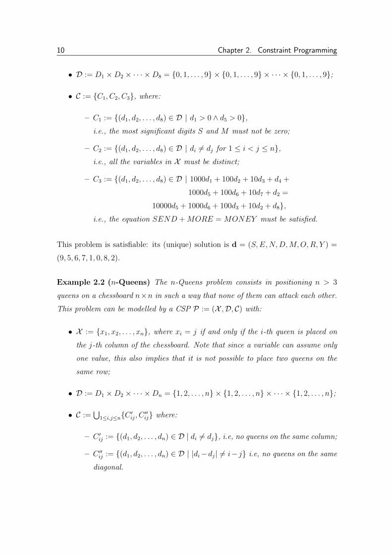
• D := D1 ×D2 × · · · ×D8 = {0, 1, . . . , 9} × {0, 1, . . . , 9} × · · · × {0, 1, . . . , 9};
• C := {C1, C2, C3}, where:
– C1 := {(d1, d2, . . . , d8) ∈ D | d1 > 0 ∧ d5 > 0},i.e., the most significant digits S and M must not be zero;
– C2 := {(d1, d2, . . . , d8) ∈ D | di 6= dj for 1 ≤ i < j ≤ n},i.e., all the variables in X must be distinct;
– C3 := {(d1, d2, . . . , d8) ∈ D | 1000d1 + 100d2 + 10d3 + d4 +
1000d5 + 100d6 + 10d7 + d2 =
10000d5 + 1000d6 + 100d3 + 10d2 + d8},i.e., the equation SEND +MORE = MONEY must be satisfied.
This problem is satisfiable: its (unique) solution is d = (S,E,N,D,M,O,R, Y ) =
(9, 5, 6, 7, 1, 0, 8, 2).
Example 2.2 (n-Queens) The n-Queens problem consists in positioning n > 3
queens on a chessboard n×n in such a way that none of them can attack each other.
This problem can be modelled by a CSP P := (X ,D, C) with:
• X := {x1, x2, . . . , xn}, where xi = j if and only if the i-th queen is placed on
the j-th column of the chessboard. Note that since a variable can assume only
one value, this also implies that it is not possible to place two queens on the
same row;
• D := D1 ×D2 × · · · ×Dn = {1, 2, . . . , n} × {1, 2, . . . , n} × · · · × {1, 2, . . . , n};
• C :=⋃
1≤i,j≤n{C ′ij, C ′′ij} where:
– C ′ij := {(d1, d2, . . . , dn) ∈ D | di 6= dj}, i.e, no queens on the same column;
– C ′′ij := {(d1, d2, . . . , dn) ∈ D | |di−dj| 6= i− j} i.e, no queens on the same
diagonal.

Chapter 2. Constraint Programming 11
For example, if n = 4 there are two solutions: d1 = (2, 4, 1, 3) and d2 = (3, 1, 4, 3).
However, since they differ only by a rotation on the chessboard, these solutions
can actually be seen as a single one. Indeed, in the n-Queens problem there is
plenty of symmetries, i.e., solutions that are identical up to symmetry operations
(rotations and reflections). Symmetries occur naturally in many problems, and it is
very important to deal with them to avoid wasting time to visit symmetric solutions,
as well as parts of the search tree which are symmetric to already visited parts. Two
common types of symmetry are variable symmetries (which act just on variables),
and value symmetries (which act just on values) [43]. One simple but highly effective
mechanism to deal with symmetry is to add constraints which eliminate symmetric
solutions [47]. An alternative way is modify the search procedure to avoid visiting
symmetric states [59, 76, 158, 63].
2.1.1 CSP on Finite Domains
Constraints can be of different types according to the domain of the variables in-
volved. For example, if p, q, r are Boolean variables we could express constraints of
the form r ≡ p∨q or p∧q → r. If n is an integer variable and X, Y are set variables,
we could consider a constraint of the form |X ∩ Y | ≤ n which constrains X and Y
to have at most n common elements. Although in theory there is no limitation on
the domains of the variables (e.g., they could be discrete, continuous, or symbolic)
the most successful CP applications are based on Finite Domains (FD), i.e., the
domain of the variables has finite cardinality. This section provides an overview of
the most widely used FD in Constraint Programming.
2.1.1.1 Boolean Variables
In CSPs with only Boolean variables, each variable can be set to either true or false.
The most common class of Boolean CSPs is represented by (Boolean, Propositional)
Satisfiability problems, better known as SAT problems [87]. In these problems the
goal is to determine if there exists an interpretation (i.e., an assignment of Boolean
12 Chapter 2. Constraint Programming
values to the variables) that satisfies a given Boolean formula.
Historically, the SAT problem was the prototype and one of the simplest NP-
complete problems [45]. It attracted a lot of attention throughout the years, and
nowadays is probably the area of greatest influence in the context of satisfiabil-
ity problems. SAT solving is commonly used in many real life problems such as
automated reasoning, computer-aided design and manufacturing, machine vision,
database, robotics, integrated circuit design, computer architecture design, and
computer network design. Its widespread use has fostered the dissemination of
a large number of different solvers [81], which success is probably due to the com-
bination of different techniques like nogoods, backjumping, and variable ordering
heuristics [142]. In particular, as we will see below, SAT solving is the CSP branch
in which portfolio approaches have been grown more. Starting from 2002, interna-
tional SAT solver competitions [111] take place in order to evaluate the performance
of different solvers on extensive benchmarks of real case, randomly generated and
hand-crafted instances defined in the Dimacs standard format [112]. It is worth not-
ing that, although technically SAT problems are simplified CSPs, in the literature
there is a clear distinction between them and the ”generic“ CSPs (which typically
have integer domains). This is because of the different nature between SAT solving
and other approaches like FD solving or Linear Programming. Henceforth, if not
better specified, with the term CSP we will refer only to generic CSPs, excluding
from such categorization the SAT problems.
There is plenty of SAT variants and related problems like 2-SAT, 3-SAT, HORN-
SAT, XOR-SAT. In particular, the Maximum Satisfiability problem (MAX-SAT) [21]
is the problem of finding an interpretation that satisfies the maximum number of
clauses. A well-known extension of SAT is Satisfiability Modulo Theories (SMT) [19]
that enriches SAT formulas with linear constraints, arrays, all-different constraints,
uninterpreted functions, and so on. These extensions typically remain NP-complete,
but efficient solvers are developing to handle such types of constraints. The SAT
problem becomes harder if we allow both existential ∃ and universal ∀ quantifica-
tion: in this case, it is called Quantified Boolean Formula problem (QBF) [35]. In

Chapter 2. Constraint Programming 13
particular, the presence of the ∀ quantifier in addition to ∃ makes the QBF problem
PSPACE-complete.
2.1.1.2 Integer Variables
For most of the problems is more natural to model a CSP with integer variables
belonging to a finite range (e.g., [−1..5] = {−1, 0, . . . , 5}) or to a disjoint union of
finite ranges (e.g., [2..8] ∪ [10..20]).3 Usually, a CSP over integers supports some
standard basic constraints (like =, 6=, <,≤, >,≥,+,−, ·, /, . . . ) together with global
constraints. A global constraint [159] can be seen as a constraint over an arbitrary
sequence of variables. The most common global constraints usually come with spe-
cific algorithms (the so-called propagators) that may help to solve a problem more
efficiently than decomposing the global constraint into basic relations. This feature
is perhaps one of the main strengths of FD solvers when solving huge combinatorial
search problems. The canonical example of a global constraint is the all-different
constraint. An all-different constraint over a set of variables states that the vari-
ables must be pairwise different. This constraint is widely used in practice and
because of its importance is offered as a built-in constraint in the large majority of
commercial and research-based constraint programming systems. In fact, although
from a purely logic point of view the semantic of all-different(x1, x2, . . . , xn) is the
same of the logic conjunction∧
1≤i,j≤n xi 6= xj, the use of a specific propagator can
make the resolution dramatically more efficient. Other examples of widely applicable
global constraints are the global cardinality constraint (gcc) [156] or the cumulative
constraint [5]. An exhaustive list of global constraints can be retrieved at [24].
Differently from SAT field, in CSP context there are fewer and less stable solvers
(e.g., see the number of entries in SAT solver competitions [25] w.r.t. CP solver
competitions [110, 139]). It should be noted that SAT problems are much easier
to encode: a CSP may contain more complex constraints (e.g., global constraints
3Note that in the literature the term ”FD solver“ refers almost always to a solver operating
on integer variables, possibly equipped with additional extensions (e.g., finite sets of integers).
Moreover, sometimes the terms ”FD solver“ and ”CP solver“ are used as synonyms.

14 Chapter 2. Constraint Programming
like bin-packing or regular). Moreover, at the moment the CP community has not
yet agreed on a standard language to encode CSP instances. The XML-based lan-
guage XCSP [161] was used to encode the input problems of the International CSP
Solver Competition (ICSC) [109]. XCSP is still used but, since the ICSC ended
in 2009, its spread over recent years has been restricted. At present, the de-facto
standard for encoding (not only) CSP problems is MiniZinc [146]. MiniZinc is cur-
rently the most used, supported, and general language to specify CP problems. It
supports also optimization problems and is the source format used in the MiniZ-
inc Challenge (MZC) [176], which is nowadays the only international competition
for evaluating the performances of CP solvers. MiniZinc is a medium-level language
that reduces the overall complexity of the higher-level language Zinc [135] by remov-
ing user-defined types, various coercions, and user-defined functions. Unlike XCSP,
MiniZinc provides the separation between model and data, is not restricted to in-
tegers, it allows if-then-else constructs, arrays, loops, varied global constraints, and
more recently it added new features like user-defined functions and option types.
FlatZinc [22] is a low-level language which is mostly a subset of MiniZinc. It is
designed for translating a general model into a specific one that has the form re-
quired by a particular solver. Indeed, starting from a solver-independent MiniZinc
model every solver can produce its own FlatZinc model by using solver-specific re-
definitions. Apart from MiniZinc, other solver-independent modelling languages are
ESRA [62], Essence [68], and OPL [180].
2.1.1.3 Other Variables
In the last years, researchers have given special attention to set variables and con-
straints. Many complex relations can be expressed with set constraints such as set
inclusion, union, intersection, disjointness, cardinality. An example of a logic-based
language for set constraints is CLP(SET ) [55]. It provides very flexible and gen-
eral forms of sets, but its effectiveness is hindered by its solving approach, which is
strongly non-deterministic. More recently, other approaches were proposed to deal
with finite sets of integers. Common ways to represent the domain of a set variable

Chapter 2. Constraint Programming 15
are the subset-bounds representation [17] and the lexicographic-bounds representa-
tion [163]. A radically different approach based on the Reduced Ordered Binary
Decision Diagrams (ROBDDs) is proposed in [95], an integration between BDD set
solvers and SAT solvers is described in [96], and a framework for combining set
variable representation is shown in [28]. Note that some FD solvers prefer to not
use set constraints, since it is possible to get equivalent formulations by making use
of only binary or integer variables.
With regard to the domain of rational and real numbers, some approaches have
been proposed especially in the context of CLP. For example, CLP(Q,R) system [99]
was developed to deal with linear (dis)equations over rational and real numbers. A
separate mention concerns instead the floating-point domain. Solving constraints
over floating-point numbers is a critical issue in numerous applications, notably in
program verification and testing. Albeit the floating-point numbers are a finite sub-
set of the real numbers, classical CSP techniques are here ineffective since the huge
size of the domains and the different properties of floating-point numbers w.r.t. real
numbers. In [137] a solver based on a conservative filtering algorithm is proposed.
In [32] the authors addressed the peculiarities of the symbolic execution of pro-
grams with floating-point numbers, while [23] proposes to use Mixed Integer Linear
programming for boosting local consistency algorithms over floating-point numbers.
The flexibility and generality of the CSP framework makes however possible its ex-
tension to non-standard domains. For example, CSPs have also been defined over
richer data types like multi-sets (or bags) [117, 182], graphs [54], strings [80] and
lattices [61].
2.1.2 CSP Solving
As mentioned earlier, solving a CSP means assigning to each variable a consistent
value of its domain. Intuitively, a trivial technique could be the systematic explo-
ration of the solutions space. This approach, also referred as “Generate & Test”, is
based on a simple idea: a complete assignment of values to variables is iteratively
generated until a (possible) solution is found. Obviously, despite this algorithm
16 Chapter 2. Constraint Programming
guarantees the completeness of the search on finite domains, it becomes intractable
very quickly when increasing the problem size. There are two main ways to improve
the efficiency of this approach: using a ”smart“ assignments generator, so as to
minimize the failures in the test phase; and merging the generator with the tester,
which is the way of CSP solving. In the last case, the consistency is tested as soon
as variables are instantiated by using a backtracking approach [136].
Backtracking is a general approach that tries to build a solution by incrementally
exploring the branches of the search space in order to extend the current partial solu-
tion (initially empty). When an inconsistency is detected, the algorithm abandons
that path and backtracks to a consistent node, thus eliminating a subspace from
the Cartesian product of the domains. Despite this pruning allows to improve the
Generate & Test approach, the running complexity of backtracking is still NP-hard
for most non-trivial problems. The three major drawbacks of standard backtracking
are: thrashing (i.e., repeated failures due to the same reason), redundant work (i.e.,
the conflicting values of variables are not remembered), and late detection (i.e., the
conflict is not detected before it really occurs). We now present an overview of some
of the major enhancements of the backtracking approach. A formal and detailed
descriptions of the following methods is outside the scope of this thesis: for more
details we refer the reader to the corresponding references.
2.1.2.1 Consistency techniques
A well-known approach for solving CSPs is based on consistency techniques. The
basic consistency techniques are based on the so called constraint (hyper) graph
—sometimes called constraints network— where nodes correspond to variables and
(hyper) edges are labelled by constraints.
Several consistency notions are reported in the literature [125, 129]. Let us fix a
problem P := (X ,D, C). The simplest consistency technique is the node-consistency
(NC), which requires that for every variable xi ∈ X , every unary constraint C
on {xi}, every d ∈ Di, we have that d ∈ C. The most widely used consistency
technique is called arc-consistency (AC). Formally, P is arc-consistent if for every

Chapter 2. Constraint Programming 17
pair of variables xi, xj, every binary constraint C on {xi, xj}, every value d ∈ Di,
there exists a value d′ ∈ Dj such that (d, d′) ∈ C . Even more invalid values can
be removed by enforcing the path-consistency (PC). Path-consistency requires that
for every triplet of variables xi, xj, xk, every C on {xi, xj}, every C ′ on {xi, xk}, and
every C ′′ on {xj, xk}, if (d, d′) ∈ C then it exists a d′′ ∈ Dk such that (d, d′′) ∈ C ′
and (d′, d′′) ∈ C ′′.It can be shown that the above consistency techniques are covered by a gen-
eral notion of (strong) k-consistency [66]. Indeed, NC is equivalent to strong 1-
consistency, AC to strong 2-consistency, and PC to strong 3-consistency. Algo-
rithms exist for making a constraint graph strongly k-consistent for k > 2, but in
practice they are rarely used because of efficiency issues. Note that virtually all the
consistency algorithms are not complete: in other terms, meeting a given notion
of consistency does not imply that the CSP is really consistent. This is because
achieving the completeness can be computationally very hard: from the practical
perspective it is preferable to settle for relaxed forms of consistency that do not
eliminate the need for search in general, but however allow to remove efficiently a
significant amount of inconsistencies.
2.1.2.2 Propagation and Search
Even if both systematic search and consistency techniques might be used alone to
completely solve CSPs, this is rarely done: a combination of both approaches is a
more common way of solving. According to a given notion of local consistency, for
each different kind of constraint suitable agents called propagators are responsible
to remove the inconsistent values in order to meet such consistency notion. A local
removal may trigger other propagators which in turn may remove values from other
domains (e.g., consider the CSP in the Example 2.3).
Example 2.3 Consider a CSP P with three variables x, y, z having domains Dx :=
[0..1], Dy := [−6..1], Dz := {1, 5} and with two constraints {x < y, y 6= z}. P is
node-consistent, but not arc-consistent. For example, if x = 1 then no value of Dy
can satisfy the constraint x < y. In order to reach the AC, the propagator of <

18 Chapter 2. Constraint Programming
reasonably assigns the values 0 to x and 1 to y; this narrowing affects y 6= z, which
becomes 1 6= z. Then, the propagator of 6= removes 1 from Dz and consequently
assign the value 5 to z.
The process of propagation is iterated until a fix-point is reached; this can happen
when the domain of a variable becomes empty (i.e., the CSP is unsatisfiable) or no
further values can be removed (i.e., the consistency notion is met). Unfortunately,
since consistency techniques are usually incomplete, there is no guarantee that once
a fix-point is reached the CSP is actually consistent. To overcome this limitation,
it is necessary to perform a search in the solutions space for to verify if there exists
a consistent assignment of values to variables. This process can be done either by
considering all the variables of X , or by performing and checking the assignments on
a proper subset L ⊂ X of so-called “labelled” variables. Different search heuristics
can be adopted and combined to speed up the search (e.g., variable choice heuristics
and value choice heuristics).
2.1.2.3 Nogood Learning and Lazy Clause Generation
In order to avoid some problems of backtracking, like thrashing and redundant
work, look-back schemes like backjumping [71] or backchecking [94] were proposed.
Typically look back schemes share the disadvantage of late detection of the conflict:
they solve the inconsistency when it occurs but do not prevent the inconsistency
to occur. Therefore, look-ahead schemes were proposed to prevent future conflicts.
Forward checking is the easiest example of a look-ahead strategy.
A very effective technique for preventing conflicts and reducing the search space
consists in learning conflicts during the search [51]. In the SAT context this is better
known as clause learning. The development and the refinement of clause learning
techniques has led to dramatic improvements for SAT solving [142]. The equivalent
of clause learning in CSP field is called nogood learning. Nogoods are redundant
constraints that in [51] are technically defined as variable assignments that are not
contained in any admissible solution. They can be learned during search, stored,
and used to prune further part of the search tree. In [115] the authors pointed out

Chapter 2. Constraint Programming 19
that nogood learning in CSP has not been as successful as clause learning in SAT,
and also proposed a generalization of standard nogoods.
There exists a lot of work proposing different techniques for encoding a CSP into
a SAT problem [4, 104, 18, 178, 174]. A hybrid approach, called Lazy Clause Gener-
ation, is instead presented in [149]. Lazy clause generation combines the strengths
of CP propagation and SAT solving. The key idea is to mimic the underlying rules
of FD propagators by properly generating corresponding SAT clauses. The clause
generation is ”lazy“ since it is not performed a priori, but it occurs during the
search. This approach enables a strong nogood learning, able to detect and analyse
the conflicts that occur during the search. Benefits of lazy clause generation on
the RCPSP/max problem are shown in [168]. Moreover, the lazy clause generation
solver Chuffed [78] has dominated the MiniZinc Challenges 2012–2014.
2.1.2.4 Local Search
The large size and the heterogeneous nature of real-world combinatorial problems
make it sometimes impracticable the use of exact approaches. A possible workaround
consists in using Local Search (LS) methods. LS methods are greedy approaches
based on a simple and general idea: trying to improve a current ”local“ solution by
moving from time to time toward a possibly better solution within a given neigh-
bourhood. If there are not better solutions in the neighbourhood, it means that
a local optimum was reached. To avoid getting stuck in a local optimum, several
effective techniques can be applied.
In [65] different hybrid methods are reported for combining the efficiency of
LS with the flexibility of CP paradigm. Some local search methods (e.g., [39, 49,
148, 152]) used CP as a way to efficiently explore large neighbourhoods with side
constraints. Others, such as [40], used LS as a way to improve the exploration of
the search tree.
In the particular context of the CSPs, a LS approach iteratively tries to improve
an assignment of the variables until all the constraints are satisfied. The local search
is therefore performed in the space D of the possible assignments, by means of a
20 Chapter 2. Constraint Programming
proper evaluation function for measuring the quality of the assignments (e.g., in
terms of the number of violated constraints).
Two main classes of local search algorithms exist. The first one is that of greedy
or non-randomized algorithms. Well-known examples of greedy algorithms are the
Hill Climbing [169] and the Tabu Search [79]. The main drawback of these algo-
rithms concerns the possibility of getting stuck in a sub-optimal state. To over-
come this problem, randomized LS algorithms has been devised. Examples of such
random-walk algorithms are the the WalkSAT/GSAT [170] and the Simulated An-
nealing [181].
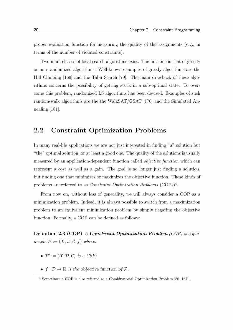
2.2 Constraint Optimization Problems
In many real-life applications we are not just interested in finding ”a” solution but
“the” optimal solution, or at least a good one. The quality of the solutions is usually
measured by an application-dependent function called objective function which can
represent a cost as well as a gain. The goal is no longer just finding a solution,
but finding one that minimizes or maximizes the objective function. These kinds of
problems are referred to as Constraint Optimization Problems (COPs)4.
From now on, without loss of generality, we will always consider a COP as a
minimization problem. Indeed, it is always possible to switch from a maximization
problem to an equivalent minimization problem by simply negating the objective
function. Formally, a COP can be defined as follows:
Definition 2.3 (COP) A Constraint Optimization Problem (COP) is a qua-
druple P := (X ,D, C, f) where:
• P ′ := (X ,D, C) is a CSP;
• f : D → R is the objective function of P.
4 Sometimes a COP is also referred as a Combinatorial Optimization Problem [86, 167].
Chapter 2. Constraint Programming 21
The goal is normally to find a solution of P ′ that minimizes f . Clearly, a COP
is more general than a CSP (that can be instead regarded as a particular COP in
which f is constant over D). For instance, a solution d found by a COP solver can
be sub-optimal (i.e., there exists at least a better solution d′ < d). Moreover, a COP
solver may find an optimal solution d∗ without being able to prove its optimality.5
Well-known examples of COPs are for instance the Cutting-stock problem [90]
(essentially reducible to the Bin-packing and Knapsack problems), the Vehicle Rout-
ing Problem (VRP) (introduced in [48] as a generalization of the Travelling Salesman
Problem (TSP) [64]), and the Resource-Constrained Project Scheduling Problem
(RCPSP) [34].
A widely used algorithm for solving COPs is called Branch and Bound (BB).
This method was first proposed in [126] for discrete programming, and has become
the most commonly used tool for solving combinatorial optimization problems. A
BB procedure consists essentially in two steps. The branching step recursively splits
the original problem into sub-problems or, in other terms, splits the search tree into
sub-trees. The bounding step instead estimates the lower and upper bounds of the
objective function f over each sub-problem. The key idea of BB algorithm is: if
the lower bound for a sub-problem P1 is greater than the upper bound for another
sub-problem P2, then P1 can be safely discarded from the search (pruning).
In the rest of the section we focus in particular on two aspects of constrained op-
timization: the so-called Soft Constraints, and the Operations Research techniques
for dealing with constrained optimization.
2.2.1 Soft Constraints
When a large set of constraints needs to be solved, it is not unlikely that there is
no way to satisfy them all: the problem is said to be over-constrained. Moreover, it
5Normally, for CP solvers the codomain of f is a finite subset of N. However, in case of non-
finite domains, a COP solver should also be able to prove the unboundedness of a problem. For
example, let us consider a simple COP defined by P := ({x},Z, ∅, f(x) := −x). In this case P is
unbounded, since f(x) is unbounded in Z.
22 Chapter 2. Constraint Programming
could be that several solutions are equally optimal. This can be caused by an inap-
propriate modelling: constraints are used to formalize desired properties rather than
preferences (i.e., conditions whose violation should be avoided as far as possible).
Soft constraints provide a way to model the preferences. In this section, inspired by
[159], we provide an overview of the most important classes and techniques of soft
constraints.
2.2.1.1 Fuzzy Constraints and Weighted CSPs
There are many classes of soft constraints. The Fuzzy Constraints approach is
based on the Fuzzy Set Theory [57, 56]. Fuzzy constraints map the preferences in
a range between 0 (total rejection) and 1 (complete acceptance). The preference
of a solution is computed by taking the minimal preference over the constraints.
This may seem counter-intuitive in some scenarios, but it is instead more natural
in others. For example, in critical settings like medical applications we would like
to be as cautious as possible. Probabilistic constraints [165] and fuzzy lexicographic
constraints [60] are variants of classical fuzzy constraints.
In other contexts we are more interested in the damages we get by not satisfy-
ing a constraint, rather than in the advantages we obtain when we satisfy it. In
Weighted Constraint Satisfaction Problems (WCSPs) each constraint is provided
with a weight representing the penalty to be paid when such constraint is violated.
An optimal solution is therefore a solution that minimizes the sum of the weights
of the violated constraints. If all the weights are set to 1, we get the MAX-CSP
problem [67]: similarly to the MAX-SAT problem, here the goal is maximizing the
number of satisfied constraints. Weighted constraints are among the most expres-
sive soft constraint frameworks, since fuzzy constraint problems can be efficiently
reduced to weighted constraint problems [166].
2.2.1.2 Formalism and Inference
The literature contains at least two general formalisms to model soft constraints:
semiring-based constraints [29, 30] and valued constraints [166]. Semiring-based

Chapter 2. Constraint Programming 23
constraints rely on a simple algebraic structure which is very similar to a semi-
ring. Valued constraints depend instead on a positive totally ordered commutative
monoid and use a different syntax w.r.t. semiring-based constraints. However, if we
assume preferences to be totally ordered [31], they have the same expressive power.
Soft constraint problems are as expressive, and as difficult to solve, as constraint
optimization problems. Indeed, given any soft constraint problem we can always
build a COP with the same solution ordering, and vice versa.
Inference in soft constraints reflects the same basic notions of classical con-
straints. Bucket elimination (BE) [52, 53] is a complete inference algorithm which
is able to compute all the optimal solutions of a soft constraint problem. The high
memory cost is the main drawback of using BE in practice. Because complete infer-
ence can be extremely time and space intensive, it is often more interesting to use
simpler but more efficient techniques of soft constraint propagation.
2.2.2 Optimization and Operations Research
In a nutshell, Operations Research (OR, also called Operational Research) is the
discipline of applying advanced analytical methods to help make better decisions.
Operations Research originated in the efforts of military planners during World
War II, and subsequently largely adopted for civilian purposes in a huge variety
of fields including business, finance, logistics, and government. OR encompasses
a wide range of problem-solving techniques and methods applied in the pursuit
of improved decision-making and efficiency, such as simulation, mathematical op-
timization, queueing theory and other stochastic-process models, Markov decision
processes, econometric methods, data envelopment analysis, neural networks, ex-
pert systems, decision analysis, and the analytic hierarchy process.6 In particular,
COPs are well studied and used in practice in areas such as services, logistics, trans-
ports, economics, and in many other industrial applications. Operations research
has proved to be useful for modelling problems of planning, routing, scheduling,
6From http://en.wikipedia.org/wiki/Operations_research.
24 Chapter 2. Constraint Programming
assignment, and design. In this section we provide an overview of the classical OR
optimization methods and a comparison between CP and OR techniques.
2.2.2.1 Linear Programming
Linear programming (LP) is a general OR optimization method in which both the
constraints and optimization function are linear. The canonical form of a LP prob-
lem is:
maximize cTx
subject to Ax ≤ b, x ≥ 0
where x ∈ Rn is the vector of the variables to be assigned, c ∈ Rn and b ∈ Rm
are vectors of known coefficients (cT is the transpose of c) while A ∈ Rm×n is the
matrix of the constraints coefficients. The inequalities Ax ≤ b are constraints that
specify a convex polyhedron (the feasible region) over which the objective function
f(x) = cTx has to be maximized.
Every LP problem (or linear program), referred to as a primal problem, can be
converted into a corresponding dual problem, which provides an upper bound to
the optimal value of the primal problem [33]. Note that the dual of a dual linear
program is the original primal linear program. Given the above definition of primal
problem, the corresponding dual is:
minimize bTy
subject to ATy ≥ c, y ≥ 0
The theory of the duality shows some interesting properties (e.g., the duality theo-
rems) and it is also exploited by the simplex algorithm [144]. This method, devised
by George Dantzig in 1947, makes use of the concept of simplex (i.e., a polytope of
n+ 1 vertices in n dimensions) for solving LP programs. Other effective techniques
for solving LP problems are instead based on interior point methods [153].
The general LP framework can be specialized according to the variables domain.
For instance, if all of the variables are required to be integers it is called an Integer

Chapter 2. Constraint Programming 25
Linear Programming (ILP) problem. In contrast to LP, which can be solved effi-
ciently in the worst case, ILP problems are in many practical situations (those with
bounded variables) NP-hard. A special case of ILP where variables are constrained
to be either 0 or 1 is the Binary Integer Programming (BIP, also called 0-1 integer
programming). Despite the binary domain of the variables, this problem is also
classified as NP-hard. If only some of the variables are required to be integers, then
the problem is called a Mixed Integer Programming (MIP) problem. These are gen-
erally NP-hard because they are even more general than ILP programs. However,
despite the NP-hardness, some important subclasses of ILP and MIP problems are
efficiently solvable. In addition to BB, other advanced algorithms for solving LP
problems include for instance the cutting-plane method and the column generation.
2.2.2.2 Nonlinear Programming
In contrast to LP, in Nonlinear Programming (NLP) problems some of the con-
straints or the objective function are nonlinear. Formally, an NLP program has the
following form:
minimize f(x)
subject to gi(x) = 0 for i = 1, 2, . . . ,m
and hj(x) ≥ 0 for j = m+ 1,m+ 2, . . . , n
where n ≥ 0 is the total number of constraints of the problem, 0 ≤ m ≤ n is the num-
ber of equalities and at least one function in {f, g1, g2, . . . , gm, hm+1, hm+2, . . . , hn}is nonlinear.
A well-known subclass of NLP problems is constituted by the Quadratic Pro-
gramming (QP) problems. A QP problem is the problem of optimizing a quadratic
function subject to linear constraints. Formally, it can be formulated as:
minimize1
2xTQx+ cTx
subject to Ax ≤ b
and Ex = d
26 Chapter 2. Constraint Programming
where x ∈ Rn represents the vector of variables; b ∈ Rm, c ∈ Rn, and d ∈ Rp are
vectors of known coefficients while A ∈ Rm×n, E ∈ Rp×n and Q ∈ Rn×n are matrices
of known coefficients (in particular, Q is symmetric).
A related programming problem, called Quadratically Constrained Quadratic
Programming (QCQP), can be posed by adding quadratic constraints on the vari-
ables. For general QP problems a variety of methods are commonly used, including
interior point, active set [143], augmented Lagrangian [44], conjugate gradient, gra-
dient projection, extensions of the simplex algorithm [143]. QP is particularly simple
when only equality constraints appear. If Q is a positive definite matrix, the ellipsoid
method solves the problem in polynomial time [123].
Operating Research vs. Constraint Programming
Roughly speaking, Operating Research and Constraint Programming can be re-
garded as different approaches for solving hard combinatorial problems. Both of
these techniques has strengths as well as weaknesses, for which reason it is not pos-
sible to determine which is the best technique to be adopted in general. As often
happens in Computer Science, some algorithms work very well on a certain class of
problems, but are ineffective for others. In these cases, often the best solution is to
use a hybrid approach able to merge the strengths of the different algorithms. CP
and OR have indeed complementary strengths: on the one hand CP provides an
easy way to deal with inference methods, logic processing, high-level problem mod-
elling and local consistency; on the other, OR works well with relaxation methods,
duality theory, atomistic problem modelling, and global consistency. Consequently,
in order to achieve better performances and solve large combinatorial problems, it
has become natural try to integrate these two approaches and the links between the
two communities have grown stronger in recent years [138].
The general advantages of CP consist in being better at sequencing and schedul-
ing, in the more natural modelling, in the use of global constraints, and in a natural
way to locally control the constraints. In contrast, CP paradigm is usually weaker
when treating discrete and continuous variables as well as over-constrained and op-

Chapter 2. Constraint Programming 27
timization problems. Moreover, this field is younger and less explored if compared
to OR. Some experimental results show that a hybrid methodology allows to signif-
icantly outperform both CP and OR for various classes of problems (e.g., planning
and scheduling-based problems) [100].
The emerging research field of the integration between OR techniques and CP
is promising and stimulating. Some of the main challenges concern the interaction
between the user and the solving process, the resolution of partially unknown or
ill-defined problems, the processing of large scale over-constrained problems, and
the improvement of the CP solving process, both in the constraints propagation and
in the solution search [138].

28 Chapter 2. Constraint Programming
Chapter 3
Portfolios of Constraint Solvers
“Multae Manus Onus Levant”1
It is well recognized in the field of Artificial Intelligence, but we could say in
Computer Science in general, that different algorithms have different performance
when solving different problems (even belonging to the same class). As pointed out
also by the “No Free Lunch” theorems [184, 185] it is evident that a single algorithm
can not be a panacea for all possible problems. Given a problem x and a collection of
different algorithms A1, A2, . . . , Am, the Algorithm Selection (AS) problem basically
consists in selecting which algorithm Ai performs better on x.
The AS problem was introduced by John R. Rice in 1976 [157]. An overall
diagram of the (refined) model he proposed is depicted in Figure 3.1. Given an
input problem x, a proper vector f(x) of real valued features is first extracted from
x. Features are essentially instance-specific attributes that characterize a given
problem. Dealing with features is crucial in AS: the idea is selecting, via a proper
selection mapping S, the best algorithm A = S(f(x)) for problem x on the basis
of the feature vector f(x). The notion of “best algorithm” is not self-contained
but defined according to suitable metrics for measuring the algorithm performance.
Formally, the performance of algorithm A on x is mapped by a performance function
P to a measure space p = P (A, x) ∈ Rn. The performance of algorithm A on x is
then a measure ‖p‖ ∈ R obtained from P (A, x) to be maximised or minimised.
1 “Many hands lighten the load”.

30 Chapter 3. Portfolios of Constraint Solvers
It is clear that this model has several degrees of freedom. For instance, how to
properly define a problem space P? What are the best features for f(x)? How to
pick an algorithm A ∈ A? Which metric is a reasonable to measure the performance
of A on x?
Figure 3.1: Refined model for the Algorithm Selection Problem (taken from [118]).
In this thesis we focus on what we could define as a particular case of AS: the
Algorithm Portfolio [84] approach applied to CP solving. The boundary between
Algorithm Selection and Algorithm Portfolios is fuzzy and these two related prob-
lems could be considered as synonyms. According to [118] definition, Algorithm
Portfolios can be seen as particular instances of the more general AS framework in
which the algorithm selection is performed case-by-case instead that in advance and
a portfolio of algorithms corresponds to the algorithm space A. In particular, within
the CP context the algorithm space consists of a portfolio {s1, s2, . . . , sm} of different
CP solvers. We can thus define a portfolio solver as a particular constraint solver
that exploits the synergy between the constituent solvers of its portfolio. When a
new unseen problem p comes, the portfolio solver tries to predict which is (or which
are) the best constituent solver(s) s1, s2, . . . , sk (k ≤ m) for solving p and then runs
such solver(s) on p.
The solver selection process is clearly a fundamental part for the success of a
portfolio approach and is usually performed by exploiting Machine Learning (ML)

Chapter 3. Portfolios of Constraint Solvers 31
techniques. ML is a broad field that uses concepts from computer science, math-
ematics, statistics, information theory, complexity theory, biology and cognitive
science in order to “construct computer programs that automatically improve with
experience”[140]. In particular, classification is a well-known ML problem that,
given a finite number of classes (or categories), consists in identifying to which class
belongs each new observation. A classifier is essentially a function mapping a new
instance —characterized by discrete or continuous features— to one class [140]. In
supervised learning a classifier is defined on the basis of a training set of instances
whose class is already known, trying to exploit such a knowledge to properly classify
each new unseen instance.
The performance measure space for a (portfolio) solver depends instead on which
kind of problems are considered. If the problem space consists of only CSPs, the
evaluation is straightforward: the outcome of a CSP solver can be either “solved”
(i.e., a solution is found or the unsatisfiability is proven) or “not solved” (i.e., the
solver gives no answer). Things become trickier when COPs are considered, since a
solver can provide sub-optimal solutions or even give the optimal one without prov-
ing its optimality. For a detailed discussion regarding different evaluation metrics
for CP solvers we refer the reader to Chapter 4 for CSPs and Chapter 5 for COPs.
In this chapter we want instead to introduce the main components that generally
characterize a CP portfolio solver, namely: the dataset of CP instances used to
make (and test) predictions, the constituent solvers of the portfolio, the features
used to characterize each CP problem, and the techniques used to properly select
and execute the constituent solvers.
3.1 Dataset
With the term dataset we will refer to what in the Rice’s model is generically referred
as the problem space P . A dataset is a data sample that should be as exhaustive
as possible, covering a significant number of problems belonging to different classes.
Gathering an adequate dataset is fundamental to build and evaluate a prediction

32 Chapter 3. Portfolios of Constraint Solvers
model:2 if the sample is not representative, it is hard to draw meaningful assess-
ments. These difficulties had already been identified in [157]: many problem spaces
are not well known and often a sample of problems is drawn from them to evaluate
empirically the performance of the given set of algorithms.
Most portfolio approaches employ ML to learn and test a prediction model. In
particular, the dataset often consists in the disjoint union of two problem spaces: a
training set and a test set. A training set is a set of already known problems used to
build the prediction model. The basic idea is to run each constituent solver on every
problem of the training set, so as to learn the information relevant to the prediction.
This process is also called training phase. A test set instead refers to a set of new,
unseen problems used to evaluate the effectiveness of the formerly trained portfolio
solver.
A well-known method for training and test a prediction model is the k-fold cross
validation [15]. In a nutshell, this method consists in partitioning the dataset D in k
disjoint folds D1,D2 . . . ,Dk such that D =⋃i=1,2,...,k Di. In turn, for i = 1, 2, . . . , k,
one fold Di is used as test set while the union⋃j 6=iDj of the remaining folds is
used as training set. In order to avoid overfitting problems (arising from prediction
models that adapt too well on the training data, rather than learning and exploiting
a generalized pattern) it is possible to randomly repeat the folds generation more
than once, then considering the average results over the repetitions. Another tech-
nique that can be effective to improve the performances accuracy consists instead
in filtering the dataset according to certain heuristics [102].
All the dataset problems should be encoded in the same solver-independent lan-
guage for being later processed by the constituent solvers. Unfortunately, as already
mentioned in 2.1.1.2, CP community has not yet agreed on a standard language to
express problem instances. If, on the one hand, the variety of languages allows for
greater flexibility and freedom of modelling, on the other hand it also represents
an obstacle for the definition and the standardisation of (portfolio) solvers. For
2 With the term “prediction model” we refer to the set of data, knowledge, and algorithms
required to predict and run the best solver(s) for solving a new CP problem.
Chapter 3. Portfolios of Constraint Solvers 33
instance, even if MiniZinc can be considered nowadays a de-facto standard, the
biggest existing dataset of CSP instances we are aware is the one used in the ICSC
2008/09, which relies on XCSP language. To overcome this limitation we developed
xcsp2mzn, a compiler from XCSP to MiniZinc language.
CSPLib [77] is a well-known library of CP problems that, however, are primarily
described in the natural language.
3.2 Solvers
A portfolio solver is composed by a number of different constituent solvers. Clearly,
each of them must support a common format in which problems are encoded. It is
of course desirable to include in the portfolio state-of-the-art and bug-free solvers.
Among the solvers that participated in the last MiniZinc Challenges, worth men-
tioning are Chuffed [78], OR-Tools [3], Opturion CPX [46], iZplus [2], Choco [1].
However, it is equally (if not more) important that the solvers are “complementary”:
they should be able to solve the greatest number of instances belonging to the most
disparate classes of problems. In other terms, an important factor for the success of
a portfolio is the marginal contribution [187] of the constituent solvers, where with
marginal contribution of a solver S we mean the difference in performance between
a portfolio solver including S and a portfolio solver excluding S.
An interesting aspect of portfolio solving concerns the size of a portfolio. As
will be observed later, we experimentally verified that increasing the number of the
constituent solvers does not necessarily imply an increase in performance of the
portfolio. In fact, even when all the constituent solvers have a potentially positive
marginal contribution, the solvers prediction could become inaccurate due to the
presence of too many candidates solvers. This scalability issue has to be taken into
account when designing a portfolio solver.
Note that a portfolio of solvers might be constituted by different parameter con-
figurations of the same solver(s). This is particularly useful when dealing with highly
parametrised solvers. The problem of automatic parameters tuning, also referred

34 Chapter 3. Portfolios of Constraint Solvers
as the Algorithm Configuration problem, has attracted some attention in recent
years. This is because with increasing of the number of parameters it becomes very
hard (even for experts) to manually tune the parameters configuration. Algorithm
configurators are also used for building portfolios. For instance, Hydra [186] and
ISAC [114] portfolio builders exploit automatic configurators like ParamILS [107],
GGA [13] or SMAC [106]. Problems of automatic building and/or configuration of
portfolios are however outside the scope of this thesis.
Although in this thesis we focus only on sequential portfolio solvers, we con-
clude this section by writing a few fords about parallel approaches on the same
multicore machine (excluding massive approaches on cluster of machines). Having
a finite portfolio, its parallelisation would seem a trivial issue: you only need to
run in parallel all the solvers. Unfortunately, often the number of the constituent
solvers exceeds the number of available cores. Furthermore, even assuming to have
fewer solvers than cores, it is likely that —due to synchronization and memory con-
sumption issues— running in parallel all the solvers on the same multicore machine
is actually far from running the same solvers on different machines [162]. A naive
multiprocessing approach could even result in wasting a huge amount of resources
for little gains (e.g., see the examples of portfolios consisting of nearly 60 solvers
in [147]). If we look at the results of the MiniZinc Challenge 2014 we notice that
—despite the availability of eight logical cores— the performance of parallel solvers
were not much better than those of sequential ones.
3.3 Features
Features are a key component in building an effective prediction model. They consist
of collections of numeric attributes that characterize a given problem. In Rice’s
model (see Figure 3.1 on page 30) a feature vector f(x) = 〈f1, f2, . . . , fm〉 for each
input problem x is extracted from a feature space F ⊆ Rm.
The choice of f(x) is arbitrary and involves various distinctions. According to
[118], a first discrimination can be made depending on the domain knowledge re-

Chapter 3. Portfolios of Constraint Solvers 35
quired to use the features. Indeed, some features may be so specific as to require
a deep knowledge of the application domain in which they are embedded. Within
the context of CP solving, some of the most common features —used for instance in
[151, 154, 188]— include statistics on the variables, the domains, the (global) con-
straints, the objective function (for COPs). Note that all such features are called
static, since they are purely syntactical and computed off-line by parsing the input
problem. Conversely, dynamic features are computed on-line by retrieving informa-
tion from short runs of a designated solver (e.g., the number of nodes explored or
the number of propagations performed). The advantage of static features is that,
unlike the dynamic ones, they are independent from the particular machine on which
they are extracted. In contrast, dynamic features also allow to take into account
some runtime information of the current problem. While some portfolios use an
hybrid approach by combining both static and dynamic features (e.g., [151, 188]),
other techniques rely on on-line features. Differently from dynamic features, on-line
features are not extracted after a short run of a designed solver: they are com-
puted directly during the search by monitoring the anytime performance of solvers
[37, 38, 172].
An important step, which can dramatically improve the predictive accuracy,
is the feature selection. Indeed, often not all the features are equally important:
the presence of uninformative features might weaken the discriminating power of
other more important features. For instance, features that are constants over the
whole dataset do not provide any useful information. The approaches based on
distance metrics like the k-Nearest Neighbours (k-NN) algorithm [6] typically scale
the features values in a reduced range. Formally, if f(x) = 〈f1, f2, . . . , fm〉 is a
feature vector, [a, b] a range of values, and li, ui are respectively the known lower
and upper bound for feature fi, then scaling a feature value fi in a range [a, b]
means mapping the original value fi ∈ [li, ui] to a scaled value f ′i ∈ [a, b]. In this
thesis we consider only linear scaling such that f ′i = a + (b− a)fi − liui − li
. The vector
f ′(x) = 〈f ′1, f ′2, . . . , f ′m〉 is also called normalized feature vector.3 Commonly choices
3 This is an abuse of notation w.r.t. the standard definition of normalized vector, commonly

36 Chapter 3. Portfolios of Constraint Solvers
for [a, b] range are [0, 1] or [−1, 1]. There exists an extensive literature regarding
the identification of the most significant features, see for example [127, 188, 154,
122, 119, 124]. It is noteworthy that feature selection is not a purely independent
process, but is instead strictly related to the dataset and the solver selectors used.
Although undoubtedly interesting, a depth analysis and evaluation of the features
is not crucial part of this thesis, where we preferred to focus on other aspects.
Finally, note that the time needed to compute features must be taken into ac-
count, since it contributes to the total solving time of a given problem. Therefore,
especially for runtime sensitive applications, all the features should be computed in
a reasonable time. For example, retrieving features from the constraint graphs may
be very time/space consuming.
3.4 Selectors
As pointed out in [118], there are many different ways to properly select one or
more constituent solver(s). Note that, even if the prediction accuracy is of course
welcome, in the CP context this requirement can be relaxed pragmatically. In a
real setting selecting a solver which is not the best one for a given instance may
be not so disadvantageous, provided that such solver is however able to solve that
instance in a reasonable time. In other words, it might be sensible to prefer the
maximization of the number of solved instances, eventually at the expense of the
solving time minimization.
Among the different selection algorithms, a primary distinction can be done
between the approaches that require to build an “explicit” prediction model and
the so called lazy approaches [118]. Lazy approaches in fact do not learn an explicit
model, but just use the set of training examples as a case base. For new problems,
a set of the k ≥ 1 closest problems in the training set is determined (via k-NN
algorithm [6]) and decisions are made accordingly. However, note that also for lazy
defined asf(x)
‖f(x)‖where ‖f(x)‖ is the norm of f(x).

Chapter 3. Portfolios of Constraint Solvers 37
approaches is necessary to keep track of the solvers execution on every instance of
the training set. In order to reduce this effort, an interesting direction is shown in
[173] where the prediction model is built by using only short runs of the constituent
solvers on the training instances.
Some lazy approaches have been studied and evaluated, see for instance [154,
151, 147, 72, 164]. Avoiding (or at least lightening) the training phase can be
advantageous in terms of simplicity and flexibility: it facilitates the treatment of
new incoming problems, solvers and features. Among lazy approaches, it is worth
mentioning the CSP portfolio solver CPHydra [151] which won the ICSC 2008.
Another rather promising lazy approach is our SUNNY, that we discuss later on in
Section 4.2.1.
However, empirical evidences prove that non-lazy techniques can be very effec-
tive. The main drawback of these approaches is that the training phase is often
sophisticated, not flexible, and computationally expensive. For instance, a state-of-
the-art SAT portfolio solver like SATzilla [190] relies on a weighted Random Forest
algorithm while 3S [113], ISAC [114], and CHSC [131] during their off-line phase
cluster the instances of the training set.
A further distinction between can be made between algorithms that select just
one solver and those that schedule more solvers within a given time window. Even
though at a first glance running in sequence more than one solver might seem not
very efficient, yet this technique has practical advantages. One of the main empirical
reasons behind this choice lies in the heavy tailed nature of solving. Indeed, many
combinatorial problems are very easy for some solvers but, at the same time, almost
impossible to solve for others. Moreover, in case a solver is not able to solve an
instance quickly, it is not unlikely that it will take a huge amount of time to solve
it. Therefore, selecting and scheduling a subset of the constituent solvers of the
portfolio instead of trying to predict the “best” one for a given instance appears
to be a good idea. This strategy ideally allows one to solve the same amount of
problems, minimizing however the risk of choosing the wrong solver. In addition,
executing more than one solver enables the communication of potentially relevant

38 Chapter 3. Portfolios of Constraint Solvers
information such as bounds, cuts or nogoods.
3.5 Related Work
We conclude this chapter by providing an overview on the related works. For com-
prehensive surveys about algorithm selection and runtime prediction, we refer the
interested reader to [171, 108]. There are also several doctoral dissertations related
to the AS problem, namely: [175, 105, 36, 69, 58, 120, 130].
Among the most promising sequential approaches in Chapter 4 we present and
evaluate in detail CPHydra [151], 3S [113], and SATZilla [190] that were gold medal-
list respectively in the ICSC 2008, the SAT Competition 2011, and the SAT Chal-
lenge 2012. In the same chapter we present ISAC [114] and SUNNY (see in particular
4.2.1).
A new SAT portfolio was proposed in [131]. This approach improves 3S since it
runs a static schedule for 10% of the available time and then executes for the re-
maining time a solver selected with a Cost-Sensitive Hierarchical Clustering (CSHC).
This solver won two gold medals in the SAT competition 2013. The CSHC approach
was not evaluated in this work since its code was not publicly available.
Apart from CPHydra and SUNNY, there are only few other approaches that can
deal with CSPs. In [14] ML techniques are used to enhance the performances of a
single CSP solver by dynamically adapting its search heuristics. These works list an
extensive set of features to train and improve the heuristics model through Support
Vector Machines. Proteus is a brand new CSP portfolio solver introduced in [104].
It does not purely rely on CSP solvers, but may decide to convert a CSP into a SAT
problem by selecting an appropriate encoding and a corresponding SAT solver.
Recalling that in this work we focus only on sequential approaches, we would
however mention some portfolio-based parallel SAT solvers like ManySAT [92], Pene-
LoPe [16] and ppfolio [160]. A parallel CP portfolio solver built on top of Numberjack
platform [98] attended the MiniZinc Challenge 2013.

Chapter 3. Portfolios of Constraint Solvers 39
The ASP field presents a lot of similarities w.r.t. the state of research in the CSP
field. Despite the development of portfolios is not as well studied as in SAT, there
exist some portfolio approaches. Worth mentioning is claspfolio [101] that also won
different tracks of the 2009 and 2011 ASP competitions.
With regard to COP portfolios, we can say that many of them are are mostly
developed just for some specific COPs like Knapsack, Most Probable Explanation,
Set Partitioning, and Travel Salesman Problem [108, 88, 179]. In [189, 114] auto-
mated algorithm configurators are used to boost the solving process. More details
about COP portfolio solvers are provided in Chapter 5.
Finally, a number of tools are being developed in order to improve portfolio
solvers usability: snappy [164] is a simple and training-less algorithm portfolio
which relies on a k-NN prediction mechanism; LLAMA (Leveraging Learning to
Automatically Manage Algorithm) [121] is instead a framework that facilitates the
exploration of different portfolio techniques on any problem domain, by supporting
the most common solver selectors and possibly combining them. To the best of
our knowledge, as shown in Chapter 6, sunny-cp is currently the only sequential
portfolio solver able to solve generic CP problems encoded in MiniZinc.

40 Chapter 3. Portfolios of Constraint Solvers

Chapter 4
Portfolios of CSP Solvers
“Satis Quod Sufficit”1
Within the SAT solving field, or at least in the context of SAT competitions,
portfolio approaches appear to be quite widespread and effective. For instance,
SATzilla [188, 190] has collected several gold medals in the SAT Competitions 2007,
2009 and the SAT Challenge 2012. 3S [113] won 7 medals in SAT Competition 2011,
while CHSC [131] won the gold medal in the Open Track of SAT Competition 2013.
Unfortunately, the dissemination of portfolios within the CSP field is much more
limited. There are several reasons for this gap between CSP and SAT. First of all,
the CSP solving field is trickier: constraints can be arbitrarily complex (e.g., global
constraints like regular or bin-packing) and some of them are supported by only a
few solvers. Moreover, no standard input language for CSP exists and there are not
exhaustive and immediately available benchmarks. These limitations somehow affect
the available CSP (portfolio) solvers. The first and the only CSP portfolio solver that
won an international competition (precisely, the ICSC 2008) was CPHydra [151].
The actual use of CPHydra is however limited, since it uses a restricted number of
dated constituent solvers and it can not deal with optimization problems. Moreover,
in [176] the authors point out that arguably the good results of CPHydra in ICSC
2008 could be attributed to the fact that the majority of the instances used in the
1 “What suffices is enough”.
42 Chapter 4. Portfolios of CSP Solvers
ICSC were publicly available before the competition. A more recent CSP portfolio
approach is Proteus [104]. It does not rely purely on CSP solvers, but may decide to
encode a CSP instance into SAT. Similarly to CPHydra, Proteus is not able to solve
COPs and still relies on the XCSP format. Conversely, given its recent introduction,
it never attended an international competition.
Given this situation, the first objective of this thesis was to shed more light on
CSP portfolio solvers. We started with a systematic study of different portfolio
approaches for CSPs, with the aim of evaluating the many different techniques and
solvers available. The first contribution —discussed in detail in Section 4.1— has
therefore been an empirical evaluation of different CSP portfolio approaches by using
the format, the dataset, and the solvers of the ICSCs 2008/2009. In particular,
in such a work we compared by means of simulations some state-of-the-art SAT
portfolios w.r.t. CPHydra and some simpler approaches built on top of some ML
classifiers.
After this first evaluation, we realized that the situation was actually changing.
The XCSP format used to model the CSPs in the ICSC has been in practice replaced
by MiniZinc [146]. New solvers supporting MiniZinc have been developed and tested
and the only active competition for evaluating CP solvers is nowadays the MiniZinc
Challenge. We therefore extended the research described in Section 4.1 by perform-
ing a more extensive evaluation. We have enhanced our previous work by evaluating
more and more recent solvers, by fully supporting the MiniZinc language (while still
retaining compatibility with XCSP), and by using a new extensive dataset of CSP
instances. Furthermore we developed SUNNY, a lazy CSP portfolio algorithm. In
Section 4.2 we provide the details of this second evaluation.
4.1 A First Empirical Evaluation
In [7] we tried to perform a first step towards the clarification of the importance of
portfolio approaches for solving CSPs. We investigated to what extent a portfolio
approach can increase the performances of a single CSP solver and which could be

Chapter 4. Portfolios of CSP Solvers 43
the best portfolio approaches, among the several existing, for solving CSPs. We
basically implemented two classes of CSP portfolio solvers, building portfolios of up
to 16 constituent solvers. In the first class we used relatively simple, off-the-shelf
ML classification algorithms in order to define the solver selectors. In the second
class we instead tried to adapt the best practice in SAT portfolio solving to the CSP
setting. In addition, we considered the aforementioned CPHydra solver.
It is worth noticing that adapting portfolios techniques from other fields is not
trivial: in most cases the lack of documentation and usability of a portfolio solver
has forced the re-implementation of (part of) the approach. Although we tried
to reproduce these approaches as faithfully as possible, they are not (and cannot
be) the original ones. For the sake of simplicity and readability, in the following
we refer to them with their original names (e.g., SATzilla or 3S) instead of using
other notational conventions (e.g., SATzilla-like or 3S-like). The rest of this section
provides a detailed description of the experiments conducted.
4.1.1 Methodology
In this section we explain the methodology and the main components used to con-
duct our experiments. All the approaches have been validated by using Intel R©Dual-
Core 2.93GHz computers with 2 GB of RAM and Ubuntu 12.04 Operating System.
The code developed to conduct the experiments is available at http://www.cs.
unibo.it/~amadini/cpaior_2013.zip.
4.1.1.1 Dataset
We tried to perform our experiments on a set of instances as realistic and large as
possible. We gathered the publicly available benchmarks of ICSC 2008, consisting
of CSPs already encoded in a normalized XCSP format.2 In addition, we added
to the dataset a number CSP instances coming from the MiniZinc 1.6 benchmarks.
In order to use these instances, we first flattened the original MiniZinc models into
2 The ICSC 2009 did not introduce new instances w.r.t. the ICSC 2008.

44 Chapter 4. Portfolios of CSP Solvers
FlatZinc (by using the standard converter mzn2fzn [145]) and we then compiled the
flattened models into XCSP (by exploiting the fzn2xcsp converter provided by the
MiniZinc suite). Unfortunately, since FlatZinc is more expressive than XCSP, we
could not convert all the models (e.g., the optimization problems were discarded).
The final dataset was built by considering 7163 instances taken from the ICSC
and 2419 instances collected from the MiniZinc benchmarks. Moreover, we discarded
all the instances solved by Mistral during the first 2 seconds computation of the
dynamic features (see Section 4.1.1.3 for more details). We thus obtained a final
dataset D containing 4547 instances encoded in XCSP language (3554 from the ICSC
and 993 from MiniZinc benchmarks).
4.1.1.2 Solvers
We decided to build our portfolios by using some of the best ranked solvers of
the ICSC, namely AbsCon (2 versions), BPSolver, Choco (2 versions), Mistral and
Sat4j. Moreover, by exploiting a specific plug-in described in [141], we were able to
use also 15 different versions of Gecode constraint solver.3 The set S of the available
constituent solvers was therefore constituted by 22 different solvers, all capable of
processing CSP instances defined in the XCSP format.
In order to perform the experiments, we run every solver of S on each problem of
the dataset D by using a solving time limit of T = 1800 seconds (the same used in
the ICSC). In total, we therefore evaluated |S×D| = 22 · 4547 = 100034 runs. Note
that 797 instances of D could not be solved by any solver of S within T seconds.
Despite most portfolio approaches tend to discard such instances from the dataset,
we instead decided to keep them. This is because we did not want to get rid of
a body of knowledge that could make a contribution in terms of solver selection
(e.g., the SUNNY algorithm that introduced in Section 4.2.1 uses a backup solver
for covering the unsolved instances).
3 Indeed, Gecode didn’t attend the competition. The different versions of Gecode have been
obtained by tuning the search parameters and the variable selection criteria.

Chapter 4. Portfolios of CSP Solvers 45
Figure 4.1a indicates the relative speed of the different solvers by showing, for
each solver, the number of instances a solver is the fastest one. As it can be seen,
Mistral is by far the best solver, since it is faster than the others for 1622 instances
(36% of D). In Figure 4.1b, following [187], we show instead a measure of the
marginal contribution of each solver, i.e., how many times a solver is able to solve
instances that no other solver can solve. Even in this case Mistral is by far the best
solver, almost one order of magnitude better than the second one. Note that there
are also eight versions of Gecode that do not give any contribution in terms of solved
instances.
(a) No. of times a solver is faster. (b) Marginal contributions.
Figure 4.1: Solvers statistics.
4.1.1.3 Features
In order to train and test the portfolio approaches, we extrapolated a set of 44
features from each instance of D. We essentially used the 36 features of CPHy-
dra [151] plus some additional features derived from the Variable Graph (VG) and
the Variable-Constraint Graph (VCG) of the XCSP instances. Whilst the majority
of these features are static, some of them are computed by collecting data from
short runs of Mistral. Among the syntactical features we can mention the number
of variables, the number of (global) constraints, the number of constants, the size of

46 Chapter 4. Portfolios of CSP Solvers
the domains and the arity of the predicates. The dynamic features instead take into
account the number of nodes explored and the number of propagations performed by
Mistral within a time limit of 2 seconds. Table 4.1 briefly summarizes the features
extracted; for a more detailed description we refer the reader to [116] since we used
them off-the-shelf and they are not a contribution of this thesis.
Dynamic features (1–4): log average variables weight, log nodes, log propagation,
log standard deviation, variables weight;
Logarithmic features (5–16): bits, boolean, constants, constraints, extra bits,
extra boolean, extra ranges, extra values, lists, ranges, search variables, values;
General purpose features (17–18): max arity, all-different constraints;
Percent features (19–28): all-different, average continuity, cumulative, decompose,
element, extensional, gac predicate, global, min continuity, weighted sum;
Perten features (29–34): average predicate arity, average predicate shape, average
predicate size, binary ext, large ext, naryext;
Square root features (35–36): average domain size, max domain size;
Additional features (37–44): ratio, reciprocal ratio, log VG average, log VG
standard deviation, log VCG average constraint, log VCG average variable, log VCG
standard deviation constraint, log VCG standard deviation variable.
Table 4.1: Features extracted by CPHydra (1–36) plus additional features (37–44).
As mentioned in 4.1.1.1, D was obtained by discarding all the problems that
Mistral solved within this 2 seconds. This is because in this case no solver selection
is needed: the instance is already solved during the features extraction. The time
needed to compute these features was often negligible: the average feature compu-
tation time was 2.47 seconds with a standard deviation of 3.54 and a maximum of
93.1 seconds.
4.1.1.4 Validation
In order to evaluate and compare the different portfolio solvers we used a 5-repeated
5-fold cross-validation (see Section 3.1 on page 31, and [15]). The dataset D was

Chapter 4. Portfolios of CSP Solvers 47
randomly partitioned in 5 disjoint folds D1,D2, . . . ,D5 by using in turn a fold Di as
the test set and the union⋃j 6=iDj of the remaining folds as the training set. To avoid
overfitting problems the random generation was repeated 5 times, thus obtaining 25
different test sets. Every test set was therefore constituted by approximately 909
instances, while every training set consisted of approximately 3638 instances.
For every instance of every test set we computed the solving strategy proposed
by a particular portfolio approach. Then, we simulated it by exploiting the already
computed runtimes, checking if the solving strategy was able to solve the instance
within T = 1800 seconds. To evaluate the performances of a (portfolio) solver we
used two metrics: the Percentage of Solved Instances (PSI) and the Average Solving
Time (AST). The PSI metric measures the percentage of instances solved by a
particular solver within the timeout T , while the AST refers to the average time
needed by a solver to solve an instance. Formally, we can define such metrics as
follows:
Definition 4.1 (proven, PSI) Let us fix a dataset D of CSPs, a set S of CSP
solvers, and a solving timeout T . Given a problem p ∈ D and a solver s ∈ S, we
define the binary function proven : S× D→ {0, 1} as:
proven(s, p) :=
1 if solver s solves the problem p in less than T seconds;
0 otherwise
Given a set of problems P ⊆ D, the PSI of solver s on P is given by:
PSI(s, P ) :=100
|P |∑p∈P
proven(s, p)
Definition 4.2 (time, AST) Let us fix a dataset D of CSPs, a set S of CSP
solvers, and a solving timeout T . Given a problem p ∈ D and a solver s ∈ S,
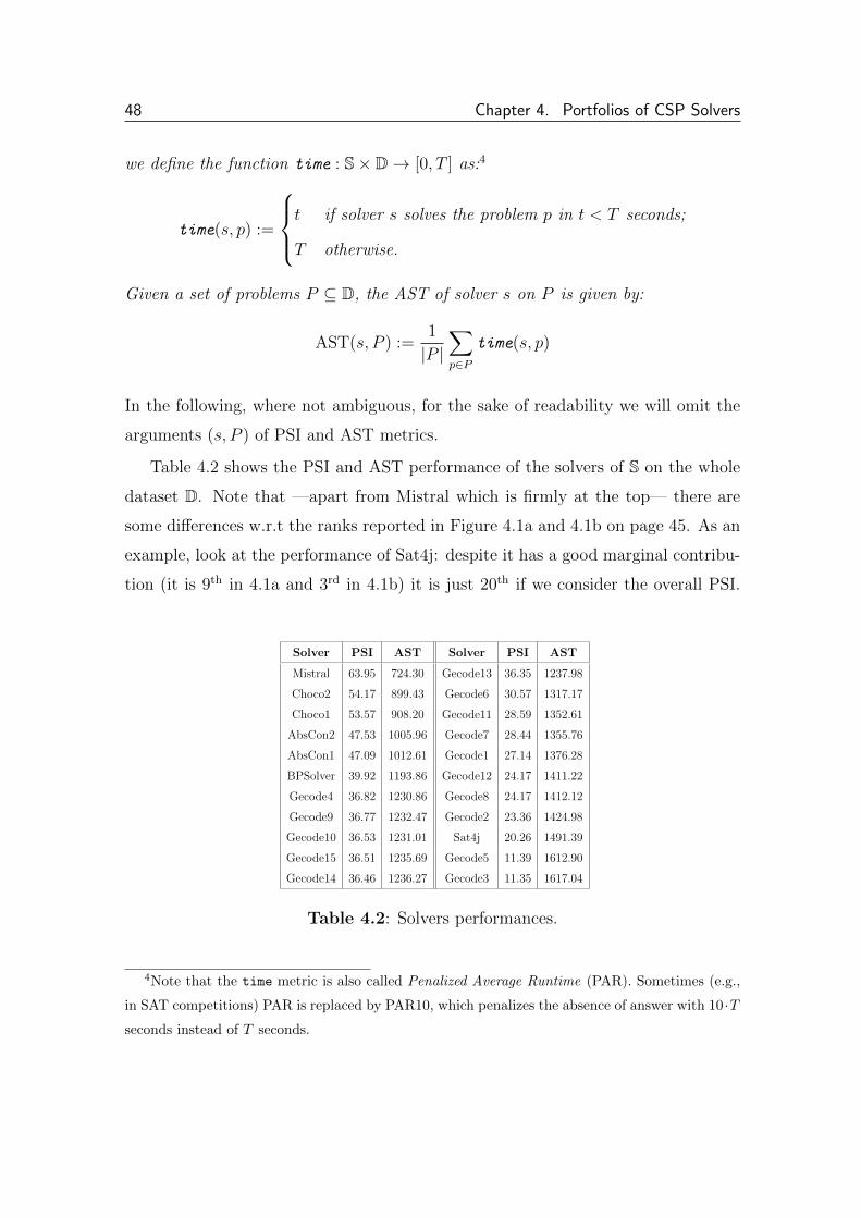
48 Chapter 4. Portfolios of CSP Solvers
we define the function time : S× D→ [0, T ] as:4
time(s, p) :=
t if solver s solves the problem p in t < T seconds;
T otherwise.
Given a set of problems P ⊆ D, the AST of solver s on P is given by:
AST(s, P ) :=1
|P |∑p∈P
time(s, p)
In the following, where not ambiguous, for the sake of readability we will omit the
arguments (s, P ) of PSI and AST metrics.
Table 4.2 shows the PSI and AST performance of the solvers of S on the whole
dataset D. Note that —apart from Mistral which is firmly at the top— there are
some differences w.r.t the ranks reported in Figure 4.1a and 4.1b on page 45. As an
example, look at the performance of Sat4j: despite it has a good marginal contribu-
tion (it is 9th in 4.1a and 3rd in 4.1b) it is just 20th if we consider the overall PSI.
Solver PSI AST Solver PSI AST
Mistral 63.95 724.30 Gecode13 36.35 1237.98
Choco2 54.17 899.43 Gecode6 30.57 1317.17
Choco1 53.57 908.20 Gecode11 28.59 1352.61
AbsCon2 47.53 1005.96 Gecode7 28.44 1355.76
AbsCon1 47.09 1012.61 Gecode1 27.14 1376.28
BPSolver 39.92 1193.86 Gecode12 24.17 1411.22
Gecode4 36.82 1230.86 Gecode8 24.17 1412.12
Gecode9 36.77 1232.47 Gecode2 23.36 1424.98
Gecode10 36.53 1231.01 Sat4j 20.26 1491.39
Gecode15 36.51 1235.69 Gecode5 11.39 1612.90
Gecode14 36.46 1236.27 Gecode3 11.35 1617.04
Table 4.2: Solvers performances.
4Note that the time metric is also called Penalized Average Runtime (PAR). Sometimes (e.g.,
in SAT competitions) PAR is replaced by PAR10, which penalizes the absence of answer with 10 ·Tseconds instead of T seconds.
Chapter 4. Portfolios of CSP Solvers 49
4.1.1.5 Portfolios composition
We pre-computed and fixed 15 portfolios Πm ⊆ S of different size m = 2, 3, . . . , 16.
Each portfolio Πm was computed by a local search algorithm aimed at maximizing
the potential PSI of Πm, breaking the ties by minimum AST.5 Note that we did not
use all the 22 solvers since we realized that for m > 16 all the portfolios potentially
solve the same number of instances (i.e., adding a new solver potentially reduces the
AST, but not increases the PSI).
The portfolios composition by varying the portfolio size is summarized in Table
4.3. Note that such a composition not necessarily reflects the ranking showed in
Figure 4.1a, 4.1b and Table 4.2. As an example, Π2 = {Mistral,AbsCon2} allows
to solve 3206 instances, while {Mistral,BPSolver} and {Mistral,Choco2} allow to
solve 3186 and 3142 instances respectively. Since even in this case Mistral is the
overall best solver, in the rest of the section it will be also called the Single Best
Solver (SBS) of the portfolio(s).
4.1.1.6 Off-the-shelf approaches
A first class of algorithms that we used as solver selectors for our evaluation is rep-
resented by what we will call the off-the-shelf (OTS) approaches. OTS approaches
are essentially ML classifiers that we use to predict the presumed best solver of the
portfolio for a given test instance. For every p ∈ D we associated a label lp corre-
sponding to the solver able to solve such instance in less time. For all the instances
not solvable by any solver of the portfolio we used a special label NO-SOLVER. The
solver designated to solve a given instance is the one predicted by the classifier. In
the cases where the solver predicted is NO-SOLVER, a pre-designated backup solver is
5Precisely, each Πm was computed by using a hill-climbing approach that, starting from an
initial random-generated portfolio Π0m, for n ≥ 1 iteratively tries to find a portfolio Πn
m of size m
that solves more instances (or solves the same number of instances more quickly) than Πn−1m . The
transition from Πn−1m to Πn
m is obtained by replacing a random subset Sn−1 ⊆ Πn−1m with a subset
Sn ⊆ S so that Πnm = (Πn−1
m \ Sn−1) ∪ Sn and |Πnm| = m.

50 Chapter 4. Portfolios of CSP Solvers
No. Solvers Portfolio Composition
2 AbsCon2 Mistral
3 Gecode15 AbsCon2 Mistral
4 Gecode15 AbsCon2 Choco2 Mistral
5 Gecode15 AbsCon2 Choco2 BPSolver Mistral
6 BPSolver Gecode15 Mistral AbsCon2 Choco2 Sat4j
7 BPSolver Gecode15 Gecode10 Mistral AbsCon2 Choco2 Sat4j
8 BPSolver Gecode15 Gecode7 Gecode10 Mistral AbsCon1 Choco2 Sat4j
9 BPSolver Gecode15 Gecode7 Gecode10 Sat4j AbsCon1 Choco1 Choco2
Mistral
10 BPSolver Gecode15 Gecode7 Gecode10 Gecode13 Sat4j AbsCon1 Choco1
Choco2 Mistral
11 BPSolver Gecode15 Gecode7 Gecode10 Gecode13 Mistral AbsCon2 AbsCon1
Choco1 Choco2 Sat4j
12 Gecode12 BPSolver Gecode15 Gecode7 Gecode10 Gecode13 Sat4j AbsCon2
AbsCon1 Choco1 Choco2 Mistral
13 Gecode9 Gecode12 BPSolver Gecode4 Gecode7 Gecode10 Gecode13 Mistral
AbsCon2 AbsCon1 Choco1 Choco2 Sat4j
14 Gecode9 Gecode12 BPSolver Gecode4 Gecode7 Gecode1 Gecode10 Gecode13
Sat4j AbsCon2 AbsCon1 Choco1 Choco2 Mistral
15 Gecode9 Gecode12 BPSolver Gecode15 Gecode4 Gecode7 Gecode1 Gecode10
Gecode13 Sat4j AbsCon2 AbsCon1 Choco1 Choco2 Mistral
16 Gecode9 Gecode12 BPSolver Gecode15 Gecode14 Gecode7 Gecode1 Gecode10
Gecode13 Sat4j AbsCon2 AbsCon1 Gecode4 Choco1 Choco2 Mistral
Table 4.3: Portfolios composition.
instead selected.6 To train and test the models we used the WEKA tool [91] which
implements some of the most well-known and widely used classification algorithms.
In particular, we used the following classifiers:
• IBk (weka.classifiers.lazy.IBk), a k-Nearest Neighbours classifier;
• DecisionStump (weka.classifiers.trees.DecisionStump), based on a de-
cision stump. Usually used in conjunction with a boosting algorithm;
• J48 (weka.classifiers.trees.J48), uses (un)pruned C4.5 decision trees;
6A backup solver is a special solver of the portfolio aimed to handle exceptional circumstances
(e.g., premature failures of other solvers). We chose Mistral as backup solver since it is the SBS of
each considered portfolio.

Chapter 4. Portfolios of CSP Solvers 51
• NaiveBayes (weka.classifiers.bayes.NaiveBayes), relies on a Naive Bayes
classifier using estimator classes;
• OneR (weka.classifiers.rules.OneR), uses the minimum-error attribute
for prediction, discretising numeric attributes;
• PART (weka.classifiers.rules.PART), exploits PART decision lists;
• Random Forest (RF) (weka.classifiers.trees.RandomForest), constructs
forests of random trees;
• SMO (weka.classifiers.functions.SMO), implements a sequential minimal
optimization algorithm for training a support vector classifier.
In order to boost the prediction accuracy, we have also used the AdaBoostM1 e
LogitBoost meta-classifiers and we performed a parameter tuning of the classifiers
configurations.7 The latter task was performed by following the best practices —
when they were available— or by manually trying different parameters starting
from the default WEKA settings. For instance, for the SMO classifier we used a
Radial Basis Function kernel and we performed a grid search over the C and γ
parameters [183].
4.1.1.7 Other approaches
The OTS approaches have been compared against CPHydra and some state-of-the-
art SAT portfolio solvers.
CPHydra [151] is the only CSP portfolio solver that won an international com-
petition.8 This solver uses a k-NN algorithm in order to compute a schedule of the
constituent solvers that maximizes the number of instances solved in the neighbour-
hood. A weak point of CPHydra is that it is not very scalable w.r.t. the number of
7 We have also tried to apply oversampling techniques (Synthetic Minority Over-sampling
Technique [41] to be precise). This however was found to be ineffective.8At the time when the experiments were conducted, CPHydra was actually the only available
CSP portfolio solver.

52 Chapter 4. Portfolios of CSP Solvers
the constituent solvers: as pointed out by its authors, “for a large number of solvers
a more sophisticated approach would be necessary”. It does not employ heuristics
for sorting the scheduled solvers and, consequently, for minimizing the solving time.
Nevertheless, by using a rather small size portfolio (3 solvers) CPHydra was able to
win the ICSC 2008.
In order to reproduce the CPHydra approach, we computed the solvers sched-
ule by exploiting the code available at http://homepages.laas.fr/ehebrard/
cphydra.html. Since this approach does not scale very well w.r.t. the size of the
portfolio we were able to simulate CPHydra only for portfolios consisting of at most
eight solvers. Note that for computing the PSI and the AST of CPHydra we did
not take into account the time it needed to compute the solvers schedule. Thus, the
results of CPHydra presented in Section 4.1.2 can be considered as an upper bound
of its real performances.
3S (SAT Solver Selector) [113] is a SAT portfolio solver that conjugates a fixed-
time static schedule with the dynamic selection of one long-running solver. Exploit-
ing the fact that a lot of SAT instances are extremely easy for one solver and almost
impossible to solve for others, 3S first executes for 10% of the time limit short runs of
its constituent solvers. The schedule of solvers, obtained by solving an optimization
problem similar to the one tackled by CPHydra, is computed offline (i.e., during the
learning phase on training data). Then, at run time, if a given instance is still not
solved a designated solver is executed for the remaining time. This solver is chosen
among the ones that are able to solve the majority of the most k-similar instances in
the training set. 3S solves the scalability issues of CPHydra because the schedule is
computed offline. Moreover, it also uses other techniques for improving the perfor-
mance of the algorithm selector. This allowed 3S to use a portfolio of 21 solvers and
to be the best-performing dynamic portfolio in the International SAT Competition
2011.
For computing the static schedule of 3S approach we did not use the original code
since it is not publicly available. We instead used the MIP solver Gurobi [89] for
solving the linear program described in [113]. In order to reduce the search space,

Chapter 4. Portfolios of CSP Solvers 53
we imposed an additional constraint requiring every solver to run for a discrete
number of seconds. In this way it was possible to get an optimal schedule of solvers
in reasonable time.9 If a problem is not solved by the static schedule in the first
T/10 = 180 seconds, we select for the remaining time the constituent solver that
solves the most instances in the k-NN neighbourhood. In order to comply with
CPHydra approach, we set k = 10.
ISAC (Instance-Specific Algorithm Configuration) is a tool aimed at optimally
tuning the configuration of an highly-parametrised solver. ISAC statically clusters
the training set by using the g-means algorithm [93] and identifies the best pa-
rameters setting for each cluster by means of GGA algorithm [13]. When a new
instance needs to be classified, ISAC determines the cluster with the nearest center
and selects the precomputed parameters for such cluster.
Thanks to the code kindly provided by Yuri Malitsky, we were able reproduce
the “Pure Solver Portfolio” approach described in [134] for SAT problems. We first
clustered the training instances and then mapped every cluster to the corresponding
best solver, i.e., the solver that solves more instances in the cluster. For every test
instance we determined the closest cluster according to the Euclidean distance and
run the corresponding best solver.
SATzilla is a SAT portfolio solver that relies on runtime prediction models to
select the solver that (hopefully) has the fastest running time on a given prob-
lem instance. In the International SAT Competition 2009, SATzilla won all the
three major tracks. More recently a new powerful version of SATzilla has been pro-
posed [190]. Instead of using regression-based runtime predictions, the newer version
uses a weighted random forest approach provided with an explicit cost-sensitive loss
function punishing misclassifications in direct proportion to their impact on portfo-
lio performance. This last version consistently outperformed the previous versions
of SATzilla and the other competitors in the SAT Challenge 2012.
We simulated the SATzilla approach by developing a MATLAB implementation
9Note that 3S uses column generation techniques to reduce the size of the problem, in spite of
the solution optimality.

54 Chapter 4. Portfolios of CSP Solvers
of the cost-sensitive classification model described in [190] with the only exception
that ties during solvers comparison are broken by selecting the solver that in general
solves the largest number of instances. We did this for simplicity: even if the code
of SATzilla is publicly available, it would have been very difficult to adapt it for our
purposes.
4.1.2 Results
We remark that in order to evaluate the performance we simulated the execution
of the solvers considering the already computed solving times. We therefore assume
that all the solvers have a deterministic behaviour. Moreover, in order to present a
more realistic scenario, the solving time of each portfolio approach also includes the
features extraction time.
In the rest of the section we present and discuss the experimental results in terms
of PSI and AST, by setting the solving timeout to T = 1800 seconds.
4.1.2.1 Percentage of Solved Instances
Figure 4.2 depicts the PSI performance of OTS approaches only, eventually boosted
by a meta classifier whenever its use improved the performance. As additional
baselines, we introduced the performance of Mistral (SBS) and of the Virtual Best
Solver (VBS), i.e., an oracle that for every instance always chooses the best solver
according to a given metric. Formally, we can define the Virtual Best Solver as
follows:
Definition 4.3 (VBS) Let us fix a dataset D of problems, a set S of solvers, and
a performance metric f : S × P → R to be maximized. We define the Virtual Best
Solver (VBS) of S (according to f) as a fictitious portfolio solver VBSf (D,S) that,
for every p ∈ D, always selects the solver s ∈ S that maximizes f(s, p).
Note that the definition of Virtual Best Solver depends only on the dataset D,
the solvers S, and the performance metric f . In particular, D may contain both

Chapter 4. Portfolios of CSP Solvers 55
2 3 4 5 6 7 8 9 10 11 12 13 14 15 1663
65
67
69
71
73
75
77
79
81
83
No. of Solvers
So
lve
d In
sta
nc
es
[%
]
(a)
2 3 4 5 6 7 8 9 10 11 12 13 14 15 1674
74.5
75
75.5
76
76.5
No. of Solvers
So
lve
d In
sta
nc
es
[%
]
(b)
Random Forest SMO AdaBoostM1 + PARTAdaBoostM1 + J48 LogitBoost + Decision Stump IBkAdaBoostM1 + OneR Naive Bayes MistralVBS
Figure 4.2: Percentage of Solved Instances of OTS approaches.
CSPs and COPs. For ease of reading, from now on we will simply use the notation
VBS in place of VBSf (D, S).
Figure 4.2b shows more in detail the best OTS approaches of Figure 4.2a.
From Figure 4.2a we can see that almost all the approaches greatly outperform
Mistral, which has a PSI of 63.95%. The only exception is the Naive Bayes classifier,
that with more than six solvers is even worse than Mistral. The VBS solves 82.47%
of the instances with a portfolio of ≥ 14 solvers, while the best OTS approach is
Random Forest (RF) that reaches a PSI of 76.65% with a portfolio of six solvers.

56 Chapter 4. Portfolios of CSP Solvers
However, Figure 4.2b shows that some other approaches are pretty close to Random
Forest: for example, SMO has a peak performance of 76.61% with a portfolio of
eight solvers.
According to the Student’s t-test [97], we have also analysed the statistical sig-
nificance of the results. We considered statistically significant two samples of data10
having a p-value less or equal than 0.05 (i.e., the probability that the observed dif-
ference is due to chance should be less than 5%). We realized that —by fixing the
portfolio size— for portfolios of size between 5 and 10 the performances of RF are
not statistically significant w.r.t. the corresponding SMO performances. Conversely,
RF is statistically better when compared to all other approaches. This confirms the
similarity of the performance between RF and SMO classifiers, as indeed can be
seen from the plots.
As far as the portfolio size is concerned, we noticed that for every classifier the
prediction becomes inaccurate after a given size. Indeed, despite the use of a larger
portfolio means that potentially more instances could be solved, we note that the
best performance has been obtained by using portfolios from 6 to 8 solvers. For some
classifiers the performance deterioration is quite significant: e.g., by using 16 solvers
the SMO classifier solves 1.22% instances less (i.e, 1.22·4547·5 / 100 ≈ 277 problems
less) than using 8 solvers. We also compared the statistical significance by fixing
an approach and varying the portfolio size. It turned out that for RF the difference
between the peak performance (obtained with 6 solvers) and the performances it
reached with k 6= 6 solvers was not statically significant only for k = 7. Similarly,
for SMO approach the only not statically significant difference is between 7 and 8
solvers (peak performance). These results confirm the intuition that it is sometimes
better to reasonably limit the portfolio size.
In Figure 4.3 we compare the performance of RF (i.e., the best OTS approach)
with those of the aforementioned 3S, CPHydra, ISAC, and SATzilla approaches.
10We define the data sample for a given portfolio solver as a binary vector (x1, x2, . . . , xn) ∈{0, 1}n corresponding to the n = 4547 · 5 = 22735 tested instances. For i = 1, 2, . . . , n, each xi is
set to 1 if and only if the portfolio solver is able to solve the instance i within the time limit T .

Chapter 4. Portfolios of CSP Solvers 57
For ease of reading, we included the VBS but not the SBS. As already stated, due
to the computational cost of computing the schedule of solvers, for CPHydra the
results are limited to a maximum of 8 solvers.
2 3 4 5 6 7 8 9 10 11 12 13 14 15 1672
74
76
78
80
82
No. of Solvers
So
lve
d In
sta
nc
es
[%
]
Random Forest Mistral 3S SATzilla
ISAC CPHydra VBS
Figure 4.3: PSI of the best approaches.
In this case it is possible to notice that the best SAT portfolio approaches, namely
3S and SATzilla, achieve the best results. 3S is able to solve slightly more instances
than SATzilla (3S has a peak PSI of 78.15% against the 78.10% peak performance
of SATzilla). Curiously enough, even though conceptually 3S and SATzilla use very
different approaches, they have very close performances. This is confirmed also from
a statistical point of view: the performance difference is not significant when using
the same portfolio. 3S and SATzilla are instead statistically better than all the
other approaches when using more than 3 solvers (e.g., 3S is able to close 26% of the
gap between Random Forest and the VBS). Moreover, their decay of performances
is less pronounced when increasing the portfolio size. As for the OTS approaches,
the best performance was reached with a relatively small portfolio (6 solvers). In
particular, the peak performances of both 3S and SATzilla are statistically significant
w.r.t. their performances with different portfolio size.

58 Chapter 4. Portfolios of CSP Solvers
CPHydra approach achieves good performance (the best is 76.81% with 6 solvers)
slightly overcoming RF and SMO. However, for 7 and 8 solvers there is a worsening
and for more than 8 solvers this approach becomes intractable.
The performances of ISAC approach are instead slightly worse than those of RF
and SMO. Indeed, ISAC reaches a maximum PSI of 75.99% (9 solvers).
4.1.2.2 Average Solving Time
Figure 4.4 shows the AST of the best approaches reported in Figure 4.3, including
also the performance of Mistral.
2 3 4 5 6 7 8 9 10 11 12 13 14 15 16350
450
550
650
750
850
950
No. of Solvers
Av
era
ge
So
lvin
g T
ime
[s
ec
.]
Random Forest Mistral 3S SATzilla
ISAC CPHydra VBS
Figure 4.4: AST of the best approaches.
There are basically two things that draw the attention in the plot. On the one
hand, for all the approaches except CPHydra one can observe a clear anti-correlation
between the PSI and the AST. In other terms, by comparing Figure 4.3 and 4.4,
it can be noted that the AST of such approaches decreases proportionally to the
increase of the PSI. This strong anti-correlation is also confirmed by the Pearson co-
efficient which is always below−0.985. The substantial break even between SATzilla

Chapter 4. Portfolios of CSP Solvers 59
and 3S is also confirmed by the fact that SATzilla is on average slightly faster than
3S (while, as seen above, 3S solves a few problems more). In particular the AST of
SATzilla is 466.82 seconds (6 solvers), against the 470.30 seconds of 3S. The VBS
instead reaches a minimum AST of 384.46 seconds with 16 solvers.
On the other hand, CPHydra behaves differently. As previously stated, this
approach was not developed for minimizing the AST and therefore it does not employ
any heuristic for deciding the ordering of the scheduled solvers. As a consequence,
CPHydra turns out to be the only portfolio solver that not minimizes the AST even
when the PSI increases. Figure 4.4 shows that the AST of CPHydra is always worse
than those of Mistral (721.03 seconds) for each portfolio size, even if its PSI is always
higher. It is therefore not surprising that CPHydra is the only approach for which
PSI and AST have a positive correlation: the Pearson coefficient between its PSI
and AST values is 0.921, denoting an almost linear relationship.
4.1.2.3 Summary
In the empirical evaluation presented in this section we have implemented and com-
pared different CSP portfolio solvers. The experimental results we got have con-
firmed the potential effectiveness of portfolio approaches also in CSP field. Indeed,
the single best solver of the portfolio was almost always significantly outperformed.
It is not surprising that the best practices in the SAT field, namely SATzilla
and 3S, are also reflected in the more general CSP setting. The considerable perfor-
mances achieved by these approaches encouraged us to combine them, by exploiting
the static solver schedule of 3S together with the dynamic selection of a long-running
solver determined by SATzilla approach. Curiously, the performances of this com-
bined approach did not improve the individual performances of 3S and SATzilla.
Another interesting fact is that, for almost all the considered portfolio approaches
except CPHydra, there is a strong anti-correlation between the average solving time
and the number of solved instances. Minimizing the average solving time in this
setting can therefore lead to solve more instances and vice versa.
60 Chapter 4. Portfolios of CSP Solvers
However, the OTS approaches are not that far from the peak performances and
—due to their simplicity— might potentially be used in dynamic scenarios were the
time to build the prediction model matters.
4.2 An Enhanced Evaluation
The extensive evaluation reported in Section 4.1 was helpful to have a general idea
of the potential benefits that portfolios might bring to CSP field. However, since
then the situation has evolved.
Firstly, the XCSP format used to model the CSPs in the ICSC has been actually
replaced by MiniZinc [146]. New solvers supporting MiniZinc have been developed
and tested, and the only remaining constraint solvers competition is nowadays the
MiniZinc Challenge [176]. A fundamental difference between XCSP and MiniZ-
inc concerns the expressiveness: unlike XCSP, MiniZinc also supports optimization
problems (which constitute about 75% of the MiniZinc Challenge problems).
Secondly, in the experiments described in Section 4.1 we reproduced and com-
pared existing portfolio approaches, but we did not introduce any new portfolio
technique.
A second contribution of this thesis is therefore a major extension of the re-
search we initiated in [7]. We performed an enhanced evaluation which extends and
improves our previous work for several reasons:
• we evaluate portfolios with more and more recent solvers;
• we fully support the MiniZinc language, while still retaining compatibility with
XCSP format;
• we use a new extensive dataset of CSP instances;
• we add to the evaluation SUNNY, a lazy portfolio approach we developed,
and sunny-csp, a prototype for a new generation CSP portfolio solver built
on top of SUNNY algorithm.

Chapter 4. Portfolios of CSP Solvers 61
In the rest of this section we explain in detail these contributions. In particular, in
Section 4.2.1 we describe the SUNNY algorithm, in Section 4.2.2 the methodology
used to conduct the new experiments, and in Section 4.2.3 the experimental results
we obtained.
4.2.1 SUNNY: a Lazy Portfolio Approach
As pointed out also by [164], probably one of the main causes of portfolios under-
utilization lies in the fact that state-of-the-art portfolio solvers usually require a
complex off-line training phase, and they are not suitably structured to incremen-
tally exploit new incoming information. For instance, SATzilla builds its prediction
model by exploiting a weighted Random Forest approach; 3S computes an off-line
schedule of solvers by exploiting column generation techniques; ISAC performs a
clustering of the training instances.
Some approaches avoiding a heavy off-line training phase have been studied and
evaluated [154, 151, 147, 72, 164]. These approaches are also referred as lazy [118].
Avoiding (or at least lightening) the training phase is advantageous in terms of
simplicity and flexibility: it facilitates the treatment of new incoming problems,
solvers and features. Unfortunately, among these lazy approaches only CPHydra
was successful enough to win a solving competition (the ICSC 2008). In Section
4.1, however, we showed that non-lazy approaches derived from SATzilla and 3S
performed better than CPHydra.
In this section we introduce SUNNY: a lazy portfolio approach for constraint
solving. SUNNY exploits instances similarity to guess the best solver(s) to use. For
a given problem p, SUNNY uses a k-Nearest Neighbours (k-NN) algorithm to select
from a training set of known instances the subset N(p, k) of the k instances closer
to p. Then, it creates a schedule of solvers by considering the smallest sub-portfolio
able to solve the maximum number of instances in the neighbourhood N(p, k). The
time allocated to each solver of the sub-portfolio is proportional to the number of
instances it solves in N(p, k).

62 Chapter 4. Portfolios of CSP Solvers
The SUNNY algorithm is described below, while an extensive evaluation and
comparison of its performance is reported in 4.2.3. Section 4.2.3.3 instead shows
sunny-csp, an effective CSP portfolio solver that relies on SUNNY algorithm.
4.2.1.1 SUNNY Algorithm
One of the main empirical observations at the base of SUNNY is that usually combi-
natorial problems are extremely easy for some solvers and, at the same time, almost
impossible to solve for others. Moreover, in case a solver is not able to solve an
instance quickly, it is likely that such solver takes a huge amount of time to solve
it. A first motivation behind SUNNY is therefore to select and schedule a subset of
the constituent solvers instead of trying to predict the “best” one for a given unseen
instance. This strategy hopefully allows one to solve the same amount of problems
minimizing the risk of choosing the wrong solver.
Another interesting consideration is that using large portfolios not always lead
to performance boost. In some cases the over-abundance of solvers hinders the
effectiveness of the considered approach. As seen in Section 4.1, and pointed out
also by [155], usually the best results are obtained by adopting a relatively small
portfolio (e.g., ten or even less solvers).
Another motivation for SUNNY is that —as witnessed for instance by the good
performance reached by CPHydra, ISAC, 3S, CSHC [131]— the “similarity assump-
tion”, stating that similar instances behave similarly, is often reasonable. It thus
makes sense to use algorithms such as k-NN to exploit the closeness between differ-
ent instances. As a side effect, this allows to relax the off-line training phase that,
as previously stated, makes the majority of the portfolio approaches rarely used in
practice.
Starting from these assumptions and driven by these motivations we developed
SUNNY, whose name is the acronym of:
• SUb-portfolio: for a given instance, we select and run a suitable sub-portfolio
(i.e., a subset of the constituent solvers of the portfolio);

Chapter 4. Portfolios of CSP Solvers 63
• Nearest Neighbours : to determine the sub-portfolio we use a k-NN algorithm
that extracts from the training set the k instances that are closer to the in-
stance to be solved;
• lazY : the approach is lazy, since no explicit prediction model is built off-line.
In a nutshell, the underlying idea behind SUNNY is to minimize the probability of
choosing the wrong solvers(s) by exploiting instance similarities in order to quickly
get the smallest possible schedule of solvers.
The pseudo-code of SUNNY is presented in Listing 4.1. SUNNY takes as input
the problem inst to be solved, the portfolio of solvers solvers, a backup solver
bkup solver, a parameter k (≥ 1) representing the neighbourhood size, a parameter
T representing the solving timeout, and a knowledge base KB of known instances for
each of which we assume to know the features and the runtimes for every solver of
the portfolio.
When a new unseen instance inst comes, SUNNY first extracts from it a proper
set of features via the function getFeatures (line 2). This function takes as input
also the knowledge base KB since the extracted features need to be preprocessed in or-
der to scale them in the range [−1, 1] and to remove the constant ones. getFeatures
returns the features vector feat vect of the instance inst. In line 3, the function
getNearestNeigbour is used to retrieve the k nearest instances similar insts to
the instance inst according to a certain distance metric (e.g., Euclidean). Then,
in line 4 the function getSubPortfolio selects the minimum subset of the portfolio
that allows to solve the greatest number of instances in the neighbourhood, by using
the average solving time for tie-breaking. Formally, fixed a timeout T , a portfolio
Π = {s1, s2, . . . , sm}, and a set of instances P = {p1, p2, . . . , pk}, we define an aux-
iliary function ϕ : P(Π) → {0, 1, . . . , k} × {0, 1, . . . ,m} × [0, T ] such that, for each
S ⊆ Π:
ϕ(S) := (k −∑p∈P
max{proven(s, p) | s ∈ S}, |S|,∑
s∈S, p∈P
time(s, p))
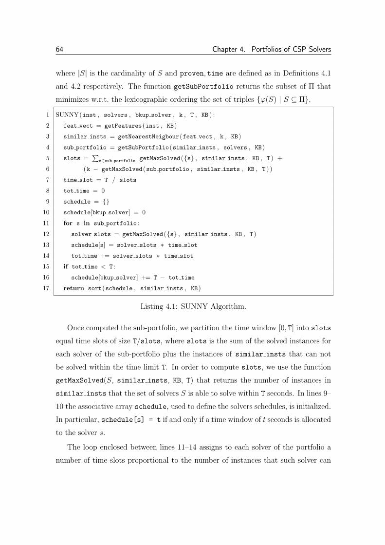
64 Chapter 4. Portfolios of CSP Solvers
where |S| is the cardinality of S and proven, time are defined as in Definitions 4.1
and 4.2 respectively. The function getSubPortfolio returns the subset of Π that
minimizes w.r.t. the lexicographic ordering the set of triples {ϕ(S) | S ⊆ Π}.
1 SUNNY(inst , solvers , bkup solver , k , T , KB ) :
2 feat vect = getFeatures(inst , KB)
3 similar insts = getNearestNeigbour(feat vect , k , KB)
4 sub portfolio = getSubPortfolio(similar insts , solvers , KB)
5 slots =∑
s∈sub portfolio getMaxSolved({s} , similar insts , KB , T) +
6 (k − getMaxSolved(sub portfolio , similar insts , KB , T ) )
7 time slot = T / slots
8 tot time = 0
9 schedule = {}10 schedule[bkup solver] = 0
11 for s in sub portfolio :
12 solver slots = getMaxSolved({s} , similar insts , KB , T)
13 schedule[s] = solver slots ∗ time slot
14 tot time += solver slots ∗ time slot
15 if tot time < T :
16 schedule[bkup solver] += T − tot time
17 return sort(schedule , similar insts , KB)
Listing 4.1: SUNNY Algorithm.
Once computed the sub-portfolio, we partition the time window [0, T] into slots
equal time slots of size T/slots, where slots is the sum of the solved instances for
each solver of the sub-portfolio plus the instances of similar insts that can not
be solved within the time limit T. In order to compute slots, we use the function
getMaxSolved(S, similar insts, KB, T) that returns the number of instances in
similar insts that the set of solvers S is able to solve within T seconds. In lines 9–
10 the associative array schedule, used to define the solvers schedules, is initialized.
In particular, schedule[s] = t if and only if a time window of t seconds is allocated
to the solver s.
The loop enclosed between lines 11–14 assigns to each solver of the portfolio a
number of time slots proportional to the number of instances that such solver can

Chapter 4. Portfolios of CSP Solvers 65
solve in the neighbourhood. In lines 15–16 the remaining time slots, corresponding
to the unsolved instances, are allocated to the backup solver. Finally, line 17 re-
turns the final schedule, obtained by sorting the solvers by average solving time in
similar insts.
Example 4.1 Let us suppose that solvers = {s1, s2, s3, s4}, bkup solver = s3,
T = 1800 seconds, k = 5, similar insts = {p1, ..., p5}, and the run-times of the
problems pi defined by KB as listed in Table 4.4.
p1 p2 p3 p4 p5
s1 T T 3 T 278
s2 T 593 T T T
s3 T T 36 1452 T
s4 T T T 122 60
Table 4.4: Runtimes (in seconds). T
indicates the timeout.
0 600 1200 1500 1800
Time [sec.]
S4 S1 S3 S2
Table 4.5: Resulting schedule of the
solvers.
The minimum size sub-portfolios that allow to solve the most instances (i.e., four
instances) are {s1, s2, s3}, {s1, s2, s4}, and {s2, s3, s4}.
SUNNY selects sub portfolio = {s1, s2, s4} since it has a lower average solving
time (1270.4 sec., to be precise). Since s1 and s4 solve two instances, s2 solves one
instance and p1 is not solved by any solver within T seconds, the time window [0, T]
is partitioned in 2 + 2 + 1 + 1 = 6 slots: two assigned to s1 and s4, one slot to s2,
and one to the backup solver s3. After sorting the solvers by average solving time in
the neighbourhood we get the schedule illustrated in Table 4.5.
Clearly, the proposed algorithm features a number of degrees of freedom. For
instance, the underlying k-NN algorithm depends on the quality of the features
extracted (and possibly filtered), on the choice of the neighbourhood size k, and on
the distance metric adopted.
66 Chapter 4. Portfolios of CSP Solvers
A potential weakness of SUNNY is that it could become impracticable for large
portfolios. Indeed, in the worst case the complexity of getSubPortfolio is expo-
nential w.r.t. the portfolio size since it has to evaluate ϕ(S) for each subset S ⊆ Π.
However, the computation of this function is almost instantaneous for portfolios
containing up to 15 solvers and, as better detailed in Section 4.2.3.3, the sizes of the
sub-portfolios are rather small for reasonable values of k.
Allocating the uncovered instances of N(p, k) to the backup solver allows the as-
signment of some slots to the (hopefully) most reliable solver. This choice obviously
biases the schedule toward the backup solver, but experimental results have proven
the effectiveness of this approach.
Finally, we want to emphasize the differences between SUNNY and CPHydra.
Although at first glance these approaches may seem pretty related (in fact, they
are both lazy approaches that apply a k-NN algorithm to compute at runtime a
schedule of the constituent solvers) there are some remarkable differences.
SUNNY puts the emphasis on finding a minimal subset of ”good” solvers. The
idea is to discard the ”bad” ones, keeping only the solver(s) that give(s) a positive
contribution in terms of solved instances. The schedule is then calculated on such
subset of good solvers, without solving any Set Covering problem as done instead
by CPHydra: only the number of instances solved in the neighbourhood matters.
We can say that SUNNY relies on a “weak” assumption of similarity, i.e.: “similar
instances are (not) solved by similar solvers”. CPHydra instead computes a schedule
that tries to maximize the number of solved instances in the neighbourhood. The
assumption of CPHydra is stronger: “similar instances have similar runtimes”.
Let us consider for instance the Example 4.1. The schedule returned by SUNNY
is [(s4, 600), (s1, 600), (s3, 300), (s2, 300)], while the one returned by CPHydra is
{s1: 716, s3: 361, s2: 600, s4: 123}.11 Note that we used a different notation for the
two schedules since CPHydra does not use heuristics for sorting the solvers. Another
11 This is the schedule returned by using the code available on-line and, in this case, by assuming
a constant distance between the problem to be solved and those of the neighbourhood. Indeed,
unlike SUNNY, CPHydra uses a weighted Euclidean distance for computing the schedule.

Chapter 4. Portfolios of CSP Solvers 67
significant difference concerns the use of a backup solver. Unlike CPHydra, SUNNY
allocates to the backup solver an amount of time proportional to the instances not
solved in the neighbourhood. If, for example, the backup solver of Example 4.1 was
s1 instead of s3, then the resulting schedule would be [(s1, 900), (s4, 600), (s2, 300)].
Finally, let us consider the time required for computing the solvers schedule.
We empirically verified that CPHydra can take a long time (much more than 1800
seconds) for portfolios of size ≥ 8. Conversely, SUNNY computes instantaneously
the solvers schedule for portfolios up to 12 solvers.
4.2.2 Methodology
Analogously to Section 4.1.1, in this section we explain the methodology used to
conduct this new evaluation. In particular, we describe the new dataset of problems,
the new solvers, and the new features we used. Even these experiments have been
performed on Intel R Dual-Core 2.93GHz computers with 2 GB of RAM and Ubuntu
12.04 Operating System. The code developed is publicly available at http://www.
cs.unibo.it/~amadini/csp_portfolio.zip.
4.2.2.1 Dataset
As already mentioned, in this evaluation we decided to switch from XCSP to MiniZ-
inc language. However, to the best of our knowledge, the biggest existing dataset
of CSP instances is still the one used in the ICSCs 2008/09. Since the CSPs of
such dataset are encoded in XCSP, we developed a compiler from XCSP to MiniZ-
inc called xcsp2mzn. Exploiting the fact that MiniZinc is more expressive than
XCSP (i.e., the majority of the primitive constraints of XCSP are also primitive
constraints of MiniZinc) the translation was pretty straightforward. The only no-
table difference concerns the compilation of extensional constraints, i.e., relations
explicitly expressed in terms of the (not) allowed tuples. This kind of constraints
are a native feature in XCSP only. In this case, we used the table global constraint
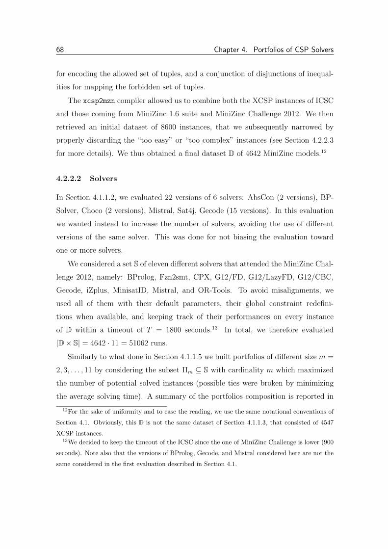
68 Chapter 4. Portfolios of CSP Solvers
for encoding the allowed set of tuples, and a conjunction of disjunctions of inequal-
ities for mapping the forbidden set of tuples.
The xcsp2mzn compiler allowed us to combine both the XCSP instances of ICSC
and those coming from MiniZinc 1.6 suite and MiniZinc Challenge 2012. We then
retrieved an initial dataset of 8600 instances, that we subsequently narrowed by
properly discarding the “too easy” or “too complex” instances (see Section 4.2.2.3
for more details). We thus obtained a final dataset D of 4642 MiniZinc models.12
4.2.2.2 Solvers
In Section 4.1.1.2, we evaluated 22 versions of 6 solvers: AbsCon (2 versions), BP-
Solver, Choco (2 versions), Mistral, Sat4j, Gecode (15 versions). In this evaluation
we wanted instead to increase the number of solvers, avoiding the use of different
versions of the same solver. This was done for not biasing the evaluation toward
one or more solvers.
We considered a set S of eleven different solvers that attended the MiniZinc Chal-
lenge 2012, namely: BProlog, Fzn2smt, CPX, G12/FD, G12/LazyFD, G12/CBC,
Gecode, iZplus, MinisatID, Mistral, and OR-Tools. To avoid misalignments, we
used all of them with their default parameters, their global constraint redefini-
tions when available, and keeping track of their performances on every instance
of D within a timeout of T = 1800 seconds.13 In total, we therefore evaluated
|D× S| = 4642 · 11 = 51062 runs.
Similarly to what done in Section 4.1.1.5 we built portfolios of different size m =
2, 3, . . . , 11 by considering the subset Πm ⊆ S with cardinality m which maximized
the number of potential solved instances (possible ties were broken by minimizing
the average solving time). A summary of the portfolios composition is reported in
12For the sake of uniformity and to ease the reading, we use the same notational conventions of
Section 4.1. Obviously, this D is not the same dataset of Section 4.1.1.3, that consisted of 4547
XCSP instances.13We decided to keep the timeout of the ICSC since the one of MiniZinc Challenge is lower (900
seconds). Note also that the versions of BProlog, Gecode, and Mistral considered here are not the
same considered in the first evaluation described in Section 4.1.

Chapter 4. Portfolios of CSP Solvers 69
Table 4.6. As can be noted, in the best case it is possible to solve at most 3698
instances. Even in this case, we kept in the dataset the 944 problems not solvable
by any solver.
Size Solvers No. of Solved Inst.
2 MinisatID, Fzn2smt 3213
3 MinisatID, Fzn2smt, OR-Tools 3549
4 MinisatID, Fzn2smt, OR-Tools, iZplus 3606
5 MinisatID, CPX, Fzn2smt, OR-Tools, iZplus 3652
6MinisatID, CPX, Fzn2smt, OR-Tools, iZplus,
3672G12/CBC
7MinisatID, CPX, Fzn2smt, OR-Tools, G12/LazyFD,
3684iZplus, G12/CBC
8MinisatID, CPX, Fzn2smt, OR-Tools, G12/LazyFD,
3692Gecode, iZplus, G12/CBC
9MinisatID, CPX, Fzn2smt, OR-Tools, G12/LazyFD,
3695Gecode, iZplus, Mistral, G12/CBC
10MinisatID, CPX, Fzn2smt, OR-Tools, G12/LazyFD,
3698Gecode, iZplus, BProlog, Mistral, G12/CBC
11MinisatID, CPX, Fzn2smt, OR-Tools, G12/LazyFD,
3698Gecode, iZplus, BProlog, G12/FD, Mistral, G12/CBC
Table 4.6: Portfolios composition. Solvers are sorted by number of solved instances.
Looking at the overall performances of the single solvers depicted in Fig. 4.5, it
can be noted that the best portfolio Πm is not always the one containing the best m
solvers in terms of PSI. Indeed, as already mentioned, an important factor for the
success of a portfolio is also the marginal contribution of every constituent solver.
Figure 4.6 depicts a measure of the marginal contribution of every solver, showing
how many times a solver can solve an instance that no other can solve.
Among all the constituent solvers, we properly elected a backup solver for each
portfolio. The choice in this case fell on MinisatID [50]14
14 We elected the backup solver by using different voting criteria, namely Borda, Approval and
Plurality. The winner, MinisatID, is also the solver that solves the greatest number of instances
within the time limit T and has the biggest marginal contribution. In the following, we will refer
to it also as the Single Best Solver (SBS).

70 Chapter 4. Portfolios of CSP Solvers
MinisatID
CPX
Fzn2smt
OR-tools
G12/LazyFD
Gecode
izplus
BProlog
G12/FD
Mistral
G12/CBC
0 500 1000 1500 2000 2500
2396
1935
1770
1423
1407
1370
1302
1148
1094
785
584
Solved Instances
So
lve
rs
Figure 4.5: Total number of solved instances for each solver of the portfolio.
MinisatID
Fzn2smt
OR-tools
izplus
CPX
G12/CBC
G12/LazyFD
Gecode
Mistral
BProlog
G12/FD
1 10 100
369
314
40
37
33
17
8
5
3
3
No. of Instances
So
lve
rs
Figure 4.6: Number of times a solver can solve an instance not solvable by any
other solver. Please note the logarithmic scale of the x axis.
4.2.2.3 Features
In Section 4.1.1.3 we exploited the features computed by Mistral solver, plus some
additional features. The point is that such features are extracted from a XCSP
specification. Since in this evaluation we switched to MiniZinc, the Mistral extractor
was no longer suitable.
In order to extract a proper set of features starting from a MiniZinc model, we
developed mzn2feat. This tool allows to compute a set of 155 different features
starting from a generic MiniZinc model. Most of these features (144) are static,
while 11 of them are dynamic (obtained by running Gecode solver for two seconds).
Although some of the features extracted by mzn2feat are quite generic (e.g.,
the number of variables or constraints), others are bound to FlatZinc language [22]

Chapter 4. Portfolios of CSP Solvers 71
(e.g., search annotations) or to Gecode (the global constraints features and the
dynamic features). An overview of the features extracted by mzn2feat is however
summarized in Table 4.7 where we denote with NV the number of variables, with
NC the number of constraints of a given problem, with min, max, avg, CV, and H
respectively the minimum, maximum, average, variation coefficient and the entropy
of a set of values. We tried to collect a set of features as large and general as
possible, obtaining a number of features that is more than triple of the Mistral
feature set introduced in Section 4.1.1.3. Obviously, not all of these features are
equally significant. We reiterate that a depth analysis and evaluation of the features
is not crucial part of this thesis. For more details about mzn2feat technicalities,
please see [145, 22, 74].
Typically, not all of the features that mzn2feat computes are equally significant.
Their importance in fact depends on the dataset and on the prediction algorithm
used for the solver selection. For example, if none of the problems contains float
variables or objective functions, then the corresponding features have no discrimi-
nant power and can be safely discarded. We thus exploited mzn2feat for extracting
a feature vector 〈f1, f2, . . . , f155〉 ∈ R155 from every problem of the initial dataset.
Following what is usually done by most of the current approaches, we removed all
the constant features from our features set and we scaled their values in the re-
duced range [−1, 1]. In this way, we associated to each problem a feature vector
〈f ′1, f ′2, . . . , f ′114〉 ∈ [−1, 1]114 consisting of 114 normalized features.
After the features extraction, we also filtered the initial dataset of 8600 instances
described in Section 4.2.2.1 by removing the “easiest” ones (i.e., those solved by
Gecode during the feature extraction when computing the dynamic features) and
the “hardest” ones (i.e., those for which the features extraction required more than
half of the timeout). We discarded these instances essentially for two reasons. First,
if an instance is already solved during the features extraction then no prediction
is needed. Second, if the feature extraction time exceeds half of the timeout it is
reasonable to assume that the recompilation of the MiniZinc model into the FlatZinc
format would end up in wasting the whole available time to solve the instance. The

72 Chapter 4. Portfolios of CSP Solvers
Variables (27): the number of variables NV ; the
number cv of constants; the number av of aliases;
the ratios av+cvNV and NV
NC ; the number of defined
variables; the number of introduced variables; the
logarithm of the product of the: variables domain
and variables degree; sum, min, max, avg, CV, and
H of the: variables domain size, variables degree,
domain size to degree ratio.
Domains (18): the number of:
boolean variables bv and the ratio bvNV ;
float variables fv and the ratio fvNV ;
integer variables iv and the ratio ivNV ;
set variables sv and the ratio svNV ;
array constraints ac and the ratio acNC ; boolean
constraints bc and the ratio bcNC ; int constraints ic
and the ratio icNC ;
float constraints fc and the ratio fcNC ;
set constraints sc and the ratio scNC .
Constraints (27): the total number of constraints
NC, the ratio NCNV , the number of constraints using
specific FlatZinc annotations (6); the logarithm of
the product of the: constraints domain and
constraints degree; sum, min, max, avg, CV, and H
of the: constraints domain, constraints degree,
domain to degree ratio.
Global Constraints (29): the total number gc of
global constraints, the ratio gcNC and the number of
global constraints for each one of the 27 equivalence
classes in which we have grouped the 47 global
constraints that Gecode natively supports.
Graphs (20): once built the Constraint Graph CG
and the Variable Graph VG we compute min, max,
avg, CV, and H of the: CG nodes degree, CG nodes
clustering coefficient, VG nodes degree, VG nodes
diameter.
Solving (11): the number of labelled variables (i.e.
the variables to be assigned); the solve goal; the
number of search annotations (3); the number of
variable choice heuristics (3); the number of value
choice heuristics (3).
Objective (12): the domain dom, the degree deg,
the ratios domdeg and deg
NC of the variable v that has to
be optimized; the degree de of v in the variable
graph, its diameter di, dedi , and di
de . Moreover,
named µdom and σdom the mean and the standard
deviation of the variables domain size and µdeg and
σdeg the mean and the standard deviation of the
variables degree, we compute domµdom
, degµdeg
, dom−µdom
σdom,
anddeg−µdeg
σdeg.
Dynamic (11): the number of solutions found; the
number p of propagations performed; the ratio pNC ;
the number e of nodes expanded in the search tree;
the number f of failed nodes in the search tree; the
ratio fe ; the maximum depth of the search stack;
the peak memory allocated; the CPU time needed
for converting from MiniZinc to FlatZinc; the CPU
time required for static features computation; the
total CPU time needed for extracting all the
features.
Table 4.7: Features extracted by mzn2feat.

Chapter 4. Portfolios of CSP Solvers 73
final dataset D was thus constituted by 4642 instances (3538 from ICSC, 6 from
MiniZinc Challenge 2012, and 1098 from MiniZinc 1.6 benchmarks).
4.2.3 Results
In this section we present the experimental results of this second evaluation. In
addition to the 3S, CPHydra, ISAC15, and SATzilla based approaches introduced
in Section 4.1.1.7 we added to the comparison also the SUNNY approach showed in
Section 4.2.1.
Regarding the OTS approaches, we used the WEKA tool for experimenting dif-
ferent techniques like oversampling, parameters tuning, meta-classifiers, and feature
selection. Unfortunately, this has not led to particularly meaningful improvements:
all the performance gains were always below 1%. We also tried to apply the filtering
techniques used in [124] but this has proved to be too time consuming (i.e., days of
computation). In this section we report only the two best OTS approaches, namely
Random Forest (RF) and SMO. The RF algorithm uses 250 decision trees, while for
SMO we got the best results with a RBF kernel and the parameters set to C = 29
and γ = 2−8.
In order to avoid discrepancies and biases, for all the other approaches using a k-
NN algorithm (viz., 3S, CPHydra, ISAC, and SUNNY) we fixed k = 10 and used the
Euclidean distance as distance metric. As done in Section 4.1, for CPHydra approach
we did not take into account the time needed for computing the solvers schedule.
We evaluated the performances of every approach in terms of AST and PSI by using
a time cap of T = 1800 seconds and a 5-repeated 5-fold cross validation. In addition
to the portfolio approaches, we included also the SBS and VBS performances.
Before presenting the results, let us dwell for a while on the ideal performances
of the perfect portfolio approach. The plot in Fig. 4.7 represents the solving time
15 ISAC is the only approach for which we employed a new version w.r.t. the one presented in
Section 4.1. Precisely, we used the version 2.0 downloadable at http://4c.ucc.ie/~ymalitsky/
Code/ISAC-Portfolio_v2.zip.
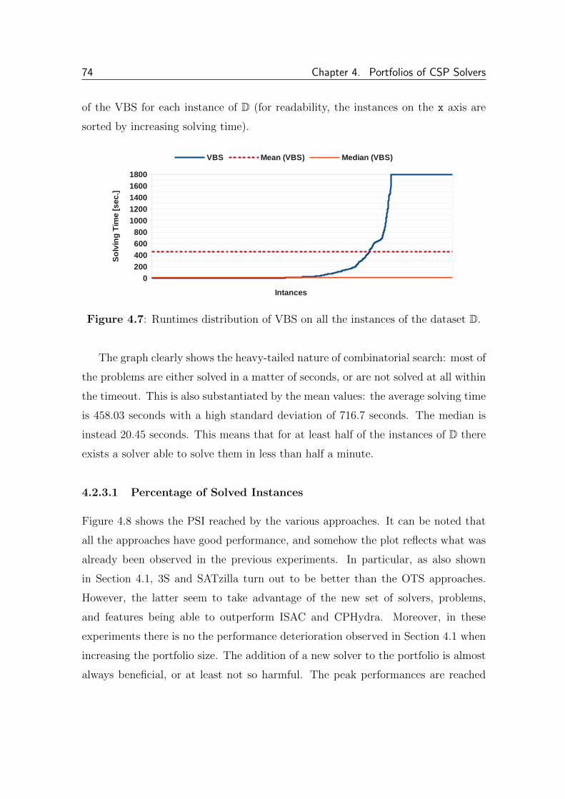
74 Chapter 4. Portfolios of CSP Solvers
of the VBS for each instance of D (for readability, the instances on the x axis are
sorted by increasing solving time).
0
200
400
600
800
1000
1200
1400
1600
1800
VBS Mean (VBS) Median (VBS)
Intances
So
lvin
g T
ime
[s
ec
.]
Figure 4.7: Runtimes distribution of VBS on all the instances of the dataset D.
The graph clearly shows the heavy-tailed nature of combinatorial search: most of
the problems are either solved in a matter of seconds, or are not solved at all within
the timeout. This is also substantiated by the mean values: the average solving time
is 458.03 seconds with a high standard deviation of 716.7 seconds. The median is
instead 20.45 seconds. This means that for at least half of the instances of D there
exists a solver able to solve them in less than half a minute.
4.2.3.1 Percentage of Solved Instances
Figure 4.8 shows the PSI reached by the various approaches. It can be noted that
all the approaches have good performance, and somehow the plot reflects what was
already been observed in the previous experiments. In particular, as also shown
in Section 4.1, 3S and SATzilla turn out to be better than the OTS approaches.
However, the latter seem to take advantage of the new set of solvers, problems,
and features being able to outperform ISAC and CPHydra. Moreover, in these
experiments there is no the performance deterioration observed in Section 4.1 when
increasing the portfolio size. The addition of a new solver to the portfolio is almost
always beneficial, or at least not so harmful. The peak performances are reached

Chapter 4. Portfolios of CSP Solvers 75
2 3 4 5 6 7 8 9 10 1166
68
70
72
74
76
78
80
VBS SUNNY CPHydra ISAC
3S SATzilla RF SMO
No. of Constituent Solvers
So
lve
d In
sta
nc
es
[%
]
Figure 4.8: PSI results considering all the approaches and the VBS.
by 3S and SUNNY while in this case SATzilla is slightly worse. Figure 4.9 depicts
the performance of 3S and SUNNY together with the VBS and the SBS. What is
immediately visible is the considerable difference in performance w.r.t. the single best
solver MinisatID. Indeed, while the SBS solves just 51.62% of the instances, the peak
performances of SUNNY and 3S (reached with 10 and 11 solvers) are respectively
77.23% and 77.69%. In particular, SUNNY is able to close up to 92.95% of the gap
between the SBS and the VBS. The peak performance of the other approaches are
instead: SATzilla 75.85% (with 9 solvers), RF 74.24% (8 solvers), SMO 74.09% (11
solvers), CPHydra 73.21% (8 solvers), ISAC 72.79% (6 solvers).
According to the Student’s t-test [97], all the peak performances are statistically
significant.
4.2.3.2 Average Solving Time
Figure 4.11 shows the Average Solving Time for each approach. The plot sub-
stantially reflects the results reported in Section 4.1. Also in this case, for all the
approaches except CPHydra, the AST is pretty anti-correlated with the PSI. It is
worth noticing that, unlike what happened in the previous experiments, 3S turns
out to be slower on average. This is due to the use of different problem instances and

76 Chapter 4. Portfolios of CSP Solvers
2 3 4 5 6 7 8 9 10 1150
55
60
65
70
75
80
VBS SBS SUNNY 3S
No. of Constituent Solvers
So
lve
d In
sta
nc
es
[%
]
Figure 4.9: PSI results considering SBS, VBS, and the best two approaches.
Figure 4.10: PSI performances.
solvers, but also to the lack in 3S of an heuristic for deciding the execution order of
the scheduled solvers. However, on average 3S results faster than CPHydra because
in 3S the solvers schedule is limited to the first 180 seconds and it solves a larger
number of instances (recall that if a solver is not able to solve a given instance,
its solving time is set to T = 1800 seconds). The heuristic used by SUNNY (the
scheduled solvers are sorted by increasing solving time in the neighbourhood) allows
it to minimize the AST and to be the overall best approach. SATzilla performances
are not so far from SUNNY, confirming that it minimizes the AST more than 3S
even when it solves less instances.
Also in this case, there is a remarkable difference between the SBS (950.91
seconds) and the best approaches (see Figure 4.12). The best AST performance,
reached by SUNNY using 10 solvers (568.84 seconds), is able to close the 77.52% of
the gap between the SBS and the VBS. Regarding ISAC, RF, and SMO, we can no-
tice the same anti-correlation with the PSI evidenced in Section 4.1. Considering all
the reported approaches, with the exception of CPHydra, the strong anti-correlation
is confirmed by the Pearson product-moment coefficient (about −0.79). There is in-
stead a strong correlation (about 0.96) between the PSI and AST of CPHydra.

Chapter 4. Portfolios of CSP Solvers 77
2 3 4 5 6 7 8 9 10 11455
505
555
605
655
705
755
805
855
SMO ISAC CPHydra SUNNY
RF SATzilla 3S VBS
No. of Constituent Solvers
So
lvin
g T
ime
[s
ec
.]
Figure 4.11: AST results considering all the approaches and the VBS.
Nonetheless, in this case the worst performance of CPHydra (884.81 seconds) how-
ever outperforms the SBS. Even it this case, all the peak performances in terms of
AST are statistically significant according with the Student’s t-test.
4.2.3.3 sunny-csp
The experimental results indicate that among the tested approaches the best per-
formance in terms of AST and PSI is reached by SUNNY. Moreover, this approach
also appears to be quite robust when varying the neighbourhood size k. Indeed, as
depicted in Fig. 4.14, varying the value of k in [5, 20] does not entail a huge im-
pact in performance (i.e., less than 1% of solved instances). The peak performance
(PSI = 77.81%) is reached with k = 16, while for k > 20 we observed a gradual
performance degradation. For instance, by using k = 25, 50, 100, 250, 500 we get a
maximum PSI of 77.59, 77.55, 77.3, 77.16, 76.56, and 72.63 respectively (see Figure
4.15). Of course, the robustness of SUNNY also depends on other factors: for in-
stance, by using different sets of solvers or instances these assessments may be no
longer be true.
However, we remark that the results so far described are based on simulations.
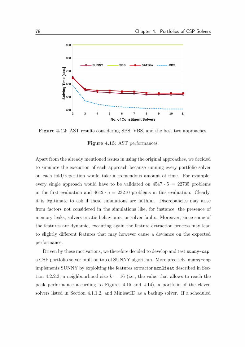
78 Chapter 4. Portfolios of CSP Solvers
2 3 4 5 6 7 8 9 10 11450
550
650
750
850
950
SUNNY SBS SATzilla VBS
No. of Constituent Solvers
So
lvin
g T
ime
[s
ec
.]
Figure 4.12: AST results considering SBS, VBS, and the best two approaches.
Figure 4.13: AST performances.
Apart from the already mentioned issues in using the original approaches, we decided
to simulate the execution of each approach because running every portfolio solver
on each fold/repetition would take a tremendous amount of time. For example,
every single approach would have to be validated on 4547 · 5 = 22735 problems
in the first evaluation and 4642 · 5 = 23210 problems in this evaluation. Clearly,
it is legitimate to ask if these simulations are faithful. Discrepancies may arise
from factors not considered in the simulations like, for instance, the presence of
memory leaks, solvers erratic behaviours, or solver faults. Moreover, since some of
the features are dynamic, executing again the feature extraction process may lead
to slightly different features that may however cause a deviance on the expected
performance.
Driven by these motivations, we therefore decided to develop and test sunny-csp:
a CSP portfolio solver built on top of SUNNY algorithm. More precisely, sunny-csp
implements SUNNY by exploiting the features extractor mzn2feat described in Sec-
tion 4.2.2.3, a neighbourhood size k = 16 (i.e., the value that allows to reach the
peak performance according to Figures 4.15 and 4.14), a portfolio of the eleven
solvers listed in Section 4.1.1.2, and MinisatID as a backup solver. If a scheduled
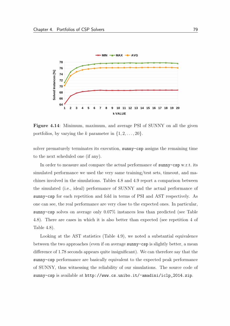
Chapter 4. Portfolios of CSP Solvers 79
1 2 3 4 5 6 7 8 9 10 11 12 13 14 15 16 17 18 19 2064
66
68
70
72
74
76
78
MIN MAX AVG
k VALUE
So
lve
d In
sta
nc
es
[%
]
Figure 4.14: Minimum, maximum, and average PSI of SUNNY on all the given
portfolios, by varying the k parameter in {1, 2, . . . , 20}.
solver prematurely terminates its execution, sunny-csp assigns the remaining time
to the next scheduled one (if any).
In order to measure and compare the actual performance of sunny-csp w.r.t. its
simulated performance we used the very same training/test sets, timeout, and ma-
chines involved in the simulations. Tables 4.8 and 4.9 report a comparison between
the simulated (i.e., ideal) performance of SUNNY and the actual performance of
sunny-csp for each repetition and fold in terms of PSI and AST respectively. As
one can see, the real performance are very close to the expected ones. In particular,
sunny-csp solves on average only 0.07% instances less than predicted (see Table
4.8). There are cases in which it is also better than expected (see repetition 4 of
Table 4.8).
Looking at the AST statistics (Table 4.9), we noted a substantial equivalence
between the two approaches (even if on average sunny-csp is slightly better, a mean
difference of 1.78 seconds appears quite insignificant). We can therefore say that the
sunny-csp performance are basically equivalent to the expected peak performance
of SUNNY, thus witnessing the reliability of our simulations. The source code of
sunny-csp is available at http://www.cs.unibo.it/~amadini/iclp_2014.zip.

80 Chapter 4. Portfolios of CSP Solvers
3 4 5 6 7 8 9 10 1174.5
75
75.5
76
76.5
77
77.5
78
K = 16K = 20K = 25K = 50K = 100K = 250
Portfolio Size
So
lve
d In
sta
nc
es
[%
]
Figure 4.15: PSI of SUNNY by varying k ∈ {16, 20, 25, 50, 100, 250}.
4.2.3.4 Training Cost
Although we evaluated the performances of different CSP portfolio solvers in terms
of PSI and AST, as done in Section 4.1 we would like to discuss shortly also the time
needed to build a prediction model. This time is not that significant and can be
omitted when measuring the actual performances of a portfolio, since the prediction
model is built offline (maybe by using powerful clusters to parallelise the workload).
However this could be no longer true when considering more dynamic scenarios, like
case-based reasoning systems that dynamically exploit new incoming knowledge to
increase their efficiency and accuracy. Obviously, all the training-based approaches
we considered might be adapted to dynamic scenarios by periodically updating the
models. However, if updating a model requires a long time (e.g., hours) the system
may be not very responsive in a dynamic context. Furthermore, some of the main
complaints about portfolios concern their poor flexibility and usability: if for winning
a competition a portfolio solver needs a year of training, it is clear that outside a
competition setting its use will result very limited.
In Figure 4.16 we report the times needed by different approaches to build the
prediction model of a single fold (928 instances) of the dataset.16 We do not consider
the lazy approaches CPHydra and SUNNY since they do not need to build and train
16We remark that these times are just an estimation since for some approaches like 3S and
SATzilla we were forced to develop a customized version. Moreover, note that such measurements
could vary (especially for approaches like 3S) according to the particular fold considered.

Chapter 4. Portfolios of CSP Solvers 81
IDEAL ACTUAL ACTUAL − IDEAL
Rep. Fold PSI AVG PSI AVG PSI AVG
1 1 75.78 75.24 −0.54
1 2 78.69 78.15 −0.54
1 3 78.77 78.77 0.00
1 4 78.13 78.23 0.11
1 5 78.23 77.92 78.13 77.70 −0.11 −0.22
2 1 78.90 79.22 0.32
2 2 76.64 76.53 −0.11
2 3 78.77 78.77 0.00
2 4 78.56 77.80 −0.75
2 5 76.08 77.79 76.08 77.68 0.00 −0.11
3 1 78.79 78.69 −0.11
3 2 76.32 76.32 0.00
3 3 78.56 78.13 −0.43
3 4 78.13 78.66 0.54
3 5 77.37 77.83 77.16 77.79 −0.22 −0.04
4 1 78.04 78.04 0.00
4 2 75.35 75.78 0.43
4 3 78.66 78.56 −0.11
4 4 78.23 78.23 0.00
4 5 78.02 77.66 77.91 77.70 −0.11 0.04
5 1 77.93 78.04 0.11
5 2 78.36 78.47 0.11
5 3 77.05 76.94 −0.11
5 4 78.56 78.45 −0.11
5 5 77.26 77.83 77.05 77.79 −0.22 −0.04
Total Average 77.81 Total Average 77.73 Total Average −0.07
Table 4.8: Percentage of Solved Instances comparison.
an explicit model.
Among the tested methods the one that employs the longest time to build a
model is SATzilla. Even though this task can be easily parallelisable, the computa-
tion for a portfolio with 11 solvers using only one machine required more than 10
minutes (about 621.55 seconds). From Figure 4.16 it can be noted that the building
time for SATzilla grows quadratically w.r.t. the portfolio size, since this approach
needs to compute for every pair of solvers a weighted random forest of decision trees.
The time needed by ISAC is instead a kind of constant but not negligible (about
400 seconds). In contrast, the time of SMO is anti-monotonic: from 102.58 to 68.29
seconds. RF instead lightly grows from 30.09 to 36.43 seconds.
As far as the 3S approach is concerned, in Figure 4.16 we present the times
needed to compute the static schedule for one fold. As already stated, this is an
NP-hard problem and its solution times may heavily depend on the specific training
data. However, for the considered fold the scheduling time turned out to be pretty
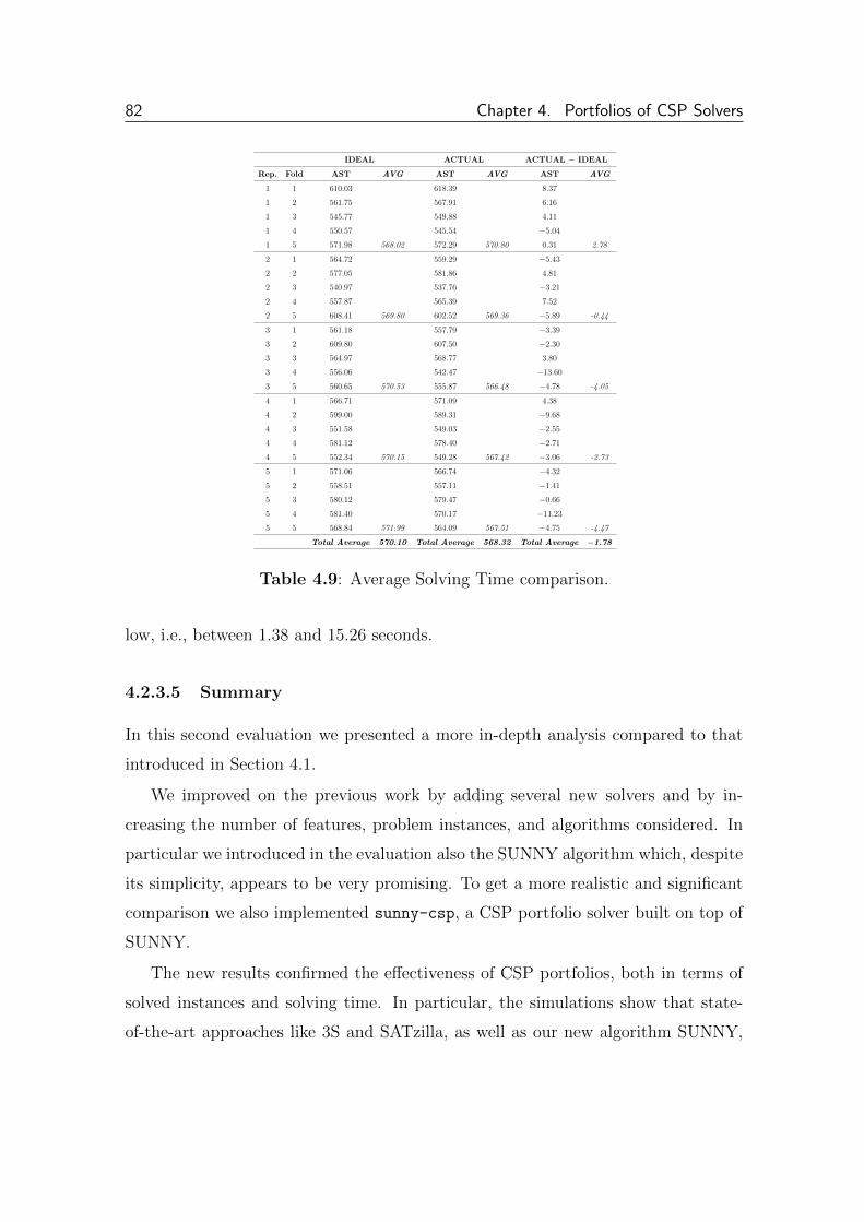
82 Chapter 4. Portfolios of CSP Solvers
IDEAL ACTUAL ACTUAL − IDEAL
Rep. Fold AST AVG AST AVG AST AVG
1 1 610.03 618.39 8.37
1 2 561.75 567.91 6.16
1 3 545.77 549.88 4.11
1 4 550.57 545.54 −5.04
1 5 571.98 568.02 572.29 570.80 0.31 2.78
2 1 564.72 559.29 −5.43
2 2 577.05 581.86 4.81
2 3 540.97 537.76 −3.21
2 4 557.87 565.39 7.52
2 5 608.41 569.80 602.52 569.36 −5.89 -0.44
3 1 561.18 557.79 −3.39
3 2 609.80 607.50 −2.30
3 3 564.97 568.77 3.80
3 4 556.06 542.47 −13.60
3 5 560.65 570.53 555.87 566.48 −4.78 -4.05
4 1 566.71 571.09 4.38
4 2 599.00 589.31 −9.68
4 3 551.58 549.03 −2.55
4 4 581.12 578.40 −2.71
4 5 552.34 570.15 549.28 567.42 −3.06 -2.73
5 1 571.06 566.74 −4.32
5 2 558.51 557.11 −1.41
5 3 580.12 579.47 −0.66
5 4 581.40 570.17 −11.23
5 5 568.84 571.99 564.09 567.51 −4.75 -4.47
Total Average 570.10 Total Average 568.32 Total Average −1.78
Table 4.9: Average Solving Time comparison.
low, i.e., between 1.38 and 15.26 seconds.
4.2.3.5 Summary
In this second evaluation we presented a more in-depth analysis compared to that
introduced in Section 4.1.
We improved on the previous work by adding several new solvers and by in-
creasing the number of features, problem instances, and algorithms considered. In
particular we introduced in the evaluation also the SUNNY algorithm which, despite
its simplicity, appears to be very promising. To get a more realistic and significant
comparison we also implemented sunny-csp, a CSP portfolio solver built on top of
SUNNY.
The new results confirmed the effectiveness of CSP portfolios, both in terms of
solved instances and solving time. In particular, the simulations show that state-
of-the-art approaches like 3S and SATzilla, as well as our new algorithm SUNNY,
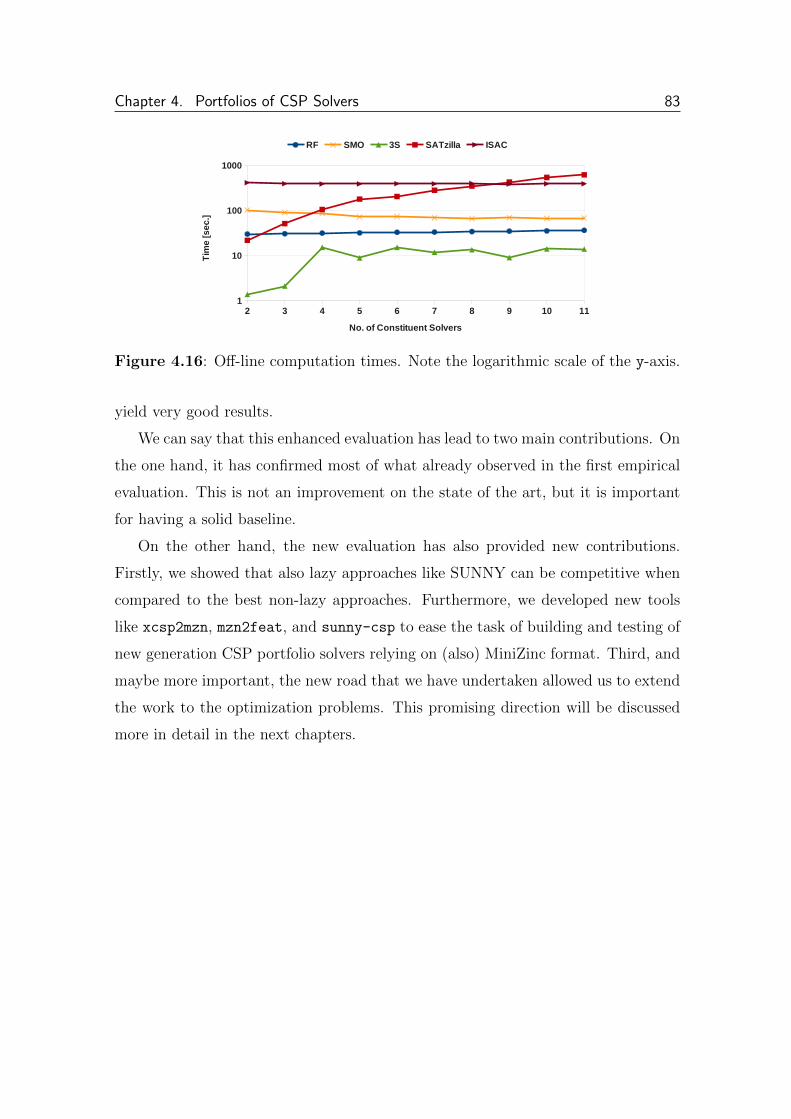
Chapter 4. Portfolios of CSP Solvers 83
2 3 4 5 6 7 8 9 10 111
10
100
1000
RF SMO 3S SATzilla ISAC
No. of Constituent Solvers
Tim
e [
se
c.]
Figure 4.16: Off-line computation times. Note the logarithmic scale of the y-axis.
yield very good results.
We can say that this enhanced evaluation has lead to two main contributions. On
the one hand, it has confirmed most of what already observed in the first empirical
evaluation. This is not an improvement on the state of the art, but it is important
for having a solid baseline.
On the other hand, the new evaluation has also provided new contributions.
Firstly, we showed that also lazy approaches like SUNNY can be competitive when
compared to the best non-lazy approaches. Furthermore, we developed new tools
like xcsp2mzn, mzn2feat, and sunny-csp to ease the task of building and testing of
new generation CSP portfolio solvers relying on (also) MiniZinc format. Third, and
maybe more important, the new road that we have undertaken allowed us to extend
the work to the optimization problems. This promising direction will be discussed
more in detail in the next chapters.

84 Chapter 4. Portfolios of CSP Solvers

Chapter 5
Portfolios of COP Solvers
“Nil Satis Nisi Optimum”1
In the previous chapter we empirically verified the benefits of using portfolio
solvers for CSPs. Unfortunately, despite the effectiveness of these approaches for
satisfaction problems, only a few studies have tried to apply portfolio techniques
to COPs. In the 2008 survey on algorithm selection procedures [171] the author
observes that: “there have been surprisingly few attempts to generalize the relevant
meta-learning ideas developed by the machine learning community, or even to fol-
low some of the directions of Leyton-Brown et al. in the constraint programming
community”. To the best of our knowledge, we think that the situation has not im-
proved significantly. In the literature just a few works deal with portfolios of COP
solvers, referring in particular to a specific problem (e.g., the Traveling Salesman
Problem [108]) or to a specific solver (e.g., by tuning its parameters [189]).
Clearly, by definition, a COP is more general than a CSP. Some issues which
are obvious for CSPs are less clear for COPs. For example, defining a suitable
metric which allows to compare different solvers is not immediate. These difficulties
explain in part the lack of exhaustive studies on portfolios consisting of different
COP solvers. Nevertheless, the COP field is clearly of particular interest. A major
contribution of this thesis is therefore the generalization of portfolio approaches from
CSPs to COPs. This chapter reports in particular two main investigations.
1 “Nothing but the best is good enough”.
86 Chapter 5. Portfolios of COP Solvers
In Section 5.1 we show a first step towards the definition of COP portfolios. Ba-
sically, we first formalized a suitable model for adapting the “classical” satisfaction-
based portfolios to address COPs, providing also some metrics to measure the solver
performance. Then, analogously to what done in Chapter 4 for CSPs, we simulated
and evaluated the performances of different COP portfolio solvers.
Similarly to Chapter 4, in Section 5.1 results are based on simulations. The point
is that a crucial difference from CSPs arises because a COP solver may yield sub-
optimal solutions before finding the best one (and possibly proving its optimality).
This means that a COP solver can transmit useful bounds information to another
one when more than one solver is selected for solving a given COP. In Section 5.2
we therefore take a step forward by addressing the problem of boosting optimization
by exploiting the sequential cooperation of different COP solvers.
5.1 An Empirical Evaluation of COP Portfolio
Approaches
In this section we tackle the problem of defining and evaluating COP portfolios. In
Section 5.1.1 we first formalize a suitable model for generalizing portfolio approaches
to COP setting. Then, by making use of an exhaustive benchmark of 2670 COP
instances, we report the performances of several portfolio approaches having differ-
ent size (from two up to twelve constituent solvers). We decided to adapt to the
optimization field the best practices according to the results presented in Chapter
4, namely: SATzilla, 3S, SUNNY. In addition, we included in the evaluation some
OTS approaches. The methodology and the portfolio algorithms we use to conduct
the tests are shown in Section 5.1.2.
The results detailed in Section 5.1.3 indicate that, also in the case of COPs,
the reported portfolio approaches almost always significantly outperform the Single
Best Solver available. In particular, we observe that the generalization of SUNNY
to COPs appears to be particularly effective: this algorithm has indeed reached the
best performances in our experiments.

Chapter 5. Portfolios of COP Solvers 87
This section is an extension of an our previous work described in [9].
5.1.1 Evaluating COP solvers
When satisfaction problems are considered, the definition and the evaluation of a
portfolio solver is pretty straightforward. Indeed, the outcome of a solver run for a
given time on a certain instance can be either ’solved’ (i.e., a solution is found or
the unsatisfiability is proven) or ’not solved’ (i.e., the solver does not say anything
about the problem). Building and evaluating a CSP solver is then conceptually
easy: the goal is to maximize the number of solved instances, solving them as fast
as possible. Unfortunately, in the COP world the dichotomy solved/not solved is
no longer suitable. A COP solver in fact can provide sub-optimal solutions or even
give the optimal one without being able to prove its optimality. Moreover, in order
to speed up the search, COP solvers could be executed in a non-independent way.
Indeed, the knowledge of a sub-optimal solution can be used by a solver to further
prune its search space and speed up the search process.
Given the proven metric typically used in the CSP field for measuring the num-
ber of solved instances (see Def. 4.1) it is possible to get a trivial generalization by
considering the number of optima proven, that is:
Definition 5.1 (proven) Let us fix a dataset D of COPs, a set S of COP solvers,
and a solving timeout T . Given a problem p ∈ D and a solver s ∈ S, we define the
binary function proven : S× D→ {0, 1} as:
proven(s, p) :=
1 if solver s proves the optimality of p in less than T seconds;
0 otherwise
Note that the concise expression “s proves the optimality of p” actually means “s
finds an optimal solution for p and proves its optimality (including proving unsat-
isfiability or unboundedness, in case)”. However, the significance of such a metric
is rather limited since it does not take into account the time taken by a solver to
prove the optimality and it excessively penalizes a solver that finds the optimal value
88 Chapter 5. Portfolios of COP Solvers
(even instantaneously) without being able to prove its optimality. One can think
to adapt the time metric defined in Section 4.1.1.4 by measuring the optimization
time instead of the solving time, i.e.:
Definition 5.2 (time) Let us fix a dataset D of COPs, a set S of COP solvers,
and a solving timeout T . Given a problem p ∈ D and a solver s ∈ S, we define the
function time : S× D→ [0, T ] as:
time(s, p) :=
t if solver s proves the optimality of p in t < T seconds;
T otherwise.
Unfortunately, even this metric is rather poor discriminating: for most of the
non-trivial optimization problems no solver may be able to prove the optimality
within a reasonable timeout. The main issue is that, although the ideal goal of
a COP solver is to prove the optimality as soon as possible, for many real life
applications it is far better to get a good solution in a relatively short time rather
than consume too much time to find the optimal value (or proving its optimality).
So, the question is: how to properly evaluate a COP solver?
An interesting method for ranking solvers is used in the MiniZinc Challenge [139].
The evaluation metric is based on a Borda count voting system [42], where each
problem is treated like a voter who ranks the solvers. Each solver gets a score
proportional to the number of solvers it beats. A solver s scores points on problem
p by comparing its performance with each other solver s′ on problem p. If s gives
a better answer than s′ then it scores 1 point, if it gives a worse solution it scores
0 points. If s and s′ give indistinguishable answers then the scoring is based on
the optimization time with a timeout of 900 seconds. In particular, s scores 0 if
it fails to find any solution or fails to prove unsatisfiability, 0.5 if both s and s′
complete the search in 0 seconds. Otherwise the score assigned to the solver s is
time(p, s′)/(time(p, s) + time(p, s′)). This metric takes into account both the best
solution found and the time needed for completing the search process, but it has
also some disadvantages. In case of indistinguishable answers, it overestimates small
time differences for easy instances, as well as underrate big time differences in case
Chapter 5. Portfolios of COP Solvers 89
of medium and hard instances. Indeed, let us suppose that two solvers s and s′
solve a problem p in 1 and 2 seconds respectively. The score assigned to s will
be 2/3 while s′ scores 1/3. However, the same score would be reached by the two
solvers if time(p, s′) = 2 time(p, s). Hence, if for example time(p, s) = 400 and
time(p, s) = 800, the difference between the scores of s and s′ would be the same
even if the absolute time difference is one second in the first case and 400 seconds
in the second. Moreover, the Borda comparisons of MiniZinc Challenge metric do
not take into account the difference in quality between distinguishable answers: the
solver that gives the worse solution always scores 0 points, regardless of whether
such solution is very close or very far from the best one.
Given these problems, in order to study the effectiveness of COP solvers (and
consequently the performance of COP portfolio solvers) we need different and more
sophisticated evaluation metrics. In the rest of this section we therefore provide an
alternative scoring system.
5.1.1.1 The score function
In order to take into account the quality of the solutions without relying on cross
comparisons between solvers, we propose the score evaluation function. The idea
of score is to evaluate the solution quality at the stroke of the solving timeout
T , by giving to each COP solver (portfolio based or not) a reward proportional
to the distance between the best solution it finds and the best known solution. An
additional reward is assigned if the optimality is proven, while a punishment is given
if no solution is found without proving unsatisfiability or unboundedness. Given a
COP instance p, we assign to a solver s a score of 1 if it proves optimality for p, 0 if
s gives no answer. Otherwise, we give to s a score corresponding to the value of its
best solution scaled into the range [α, β] where α and β are two arbitrary parameters
such that 0 ≤ α ≤ β ≤ 1. Intuitively, the parameters α and β map respectively the
value of the worst and the best known solution of the known COP solvers at the
timeout T .
In order to formally define this scoring function and to evaluate the quality

90 Chapter 5. Portfolios of COP Solvers
of a solver, we need some preliminary definitions. Let S be the set of the available
solvers (possibly including portfolio solvers), D a dataset of COP problems and T the
solving timeout. We use the function sol(s, p, t) : S× D× [0, T ]→ {unk, sat, opt}to map the outcome of a solver s for a problem p at time t. In particular, sol(s, p, t)
is either unk, if s gives no answer about p; sat, if s finds a solution for p without
proving the optimality; opt if it proves the optimality. Similarly, we use the function
val : S × D × [0, T ] → R ∪ {+∞} to define the values of the objective function.
In particular, val(s, p, t) is the best objective value found by solver s for instance p
at time t (if no solution is found at that time, val(s, p, t) = +∞). We assume the
solvers behave (anti-)monotonically, i.e., as time goes the solution quality gradually
improves and never degrades:2
∀ s ∈ S : ∀ p ∈ D : ∀ t, t′ ∈ [0, T ] : t ≤ t′ =⇒ val(s, p, t′) ≤ val(s, p, t).
We are now ready to define a measure that quantitatively represents how good the
solver s is when solving problem p over time t.
Definition 5.3 (score) Let us fix two parameters α, β ∈ [0, 1], a dataset D of
COPs, a set S of COP solvers, and a solving timeout T . We define the scoring
value of s (shortly, score) on the instance p at a given time t as a parametric
function scoreα,β : S× D× [0, T ]→ [0, 1] defined as follows:
scoreα,β(s, p, t) :=
0 if sol(s, p, t) = unk;
1 if sol(s, p, t) = opt;
β if sol(s, p, t) = sat ∧minVp = maxVp;
max
{β − (β − α) · val(s, p, t)−minVp
maxVp −minVp, 0
}otherwise.
where Vp = {val(s, p, T ) : s ∈ S} is the set of the objective function values found
by any solver s at the time limit T .3
2We can omit non-monotonic entry, if any. Recall that, without loss of generality, we consider
only minimization problems.3 Note that a portfolio solver executing more than one solver for t < T seconds could produce

Chapter 5. Portfolios of COP Solvers 91
The score of a solver is therefore a measure in the range [0, 1] that is linearly
dependent on the distance between the best solution it finds and the best solutions
found by every other available solver. To better clarify the score definition, consider
the Example 5.1.
Example 5.1 Let us consider the scenario in Figure 5.1 depicting the performances
of three different solvers run on the same minimization problem.
500 800 1000Time [seconds]
70
60
50
40
30
20
10
Solutio
n Va
lue
s1
s2
s3
Figure 5.1: Solvers performance example.
By choosing T = 500 as time limit, α = 0.25, and β = 0.75, the score assigned
to s1 is 0.75 because it finds the solution with minimum value (40), the score of s2
is 0.25 since it finds the solution with maximum value (50), and the score of s3 is
0 because it does not find a solution in T seconds. If instead T = 800, the score
assigned to s1 becomes 0.75− (40− 10) · 0.5/(50− 10) = 0.375 while the score of s2
is 0.25 and the score of s3 is 0.75. If T = 1000, since s3 proves the optimality of the
value 10 at time 900 (see the point marked with a star in Figure 5.1) it receives a
corresponding reward reaching then the score 1.
a solution that is outside the range [minVp,maxVp], potentially generating a score lower than α
(and even lower than zero). The latter case however is very uncommon: in our experiments we
noticed that the 0 score was assigned only to the solvers that did not find any solution.

92 Chapter 5. Portfolios of COP Solvers
Being score a parametric function, it obviously also depends on the α and β
parameters. Among all the possible choices, we found it reasonable to set α = 0.25
and β = 0.75. In this way, we halved the codomain: one half (i.e., the range
[0.25, 0.75]) is intended to map the quality of the sub-optimal solutions, while the
other half consists of two “gaps” (i.e., the intervals [0, 0.25] and [0.75, 1]) that are
meant to either penalize the lack of solutions or to reward the proven optimality.
In the following, unless otherwise specified, we will simply use the notation score
(or simply score) to indicate the function score0.25,0.75. As one can imagine, other
thresholds would have been equally justifiable. Even though a systematic study of
the impact of α and β parameters is outside the scope of this work, in the following
we will also report the results obtained by using the score0,1 function (see Section
5.1.3.1). Furthermore, with a little abuse of notation, we will use the short notation
score(s, p) in place of score(s, p, T ), where T is the solving timeout.
5.1.2 Methodology
Taking as baseline the methodology and the results of Chapter 4, in this section we
present the main ingredients and the procedure that we have used for conducting
our experiments and for evaluating the COP portfolios.
5.1.2.1 Solvers, Dataset, and Features
We built the set S of the single solvers used to define our portfolios by exploiting 12
solvers of the MiniZinc Challenge 2012, namely: BProlog, Fzn2smt, CPX, G12/FD,
G12/LazyFD, G12/MIP, Gecode, izplus, JaCoP, MinisatID, Mistral and OR-Tools.
We used all of them with their default parameters, their global constraint redefini-
tions when available, and keeping track of each solution found by every solver within
the timeout of the MiniZinc Challenge, i.e., T = 900 seconds.
To conduct our experiments on a dataset of instances as realistic and large as
possible, we have considered all the COPs of the MiniZinc 1.6 benchmark [146]. We
also added all the instances of the MiniZinc Challenge 2012 thus obtaining an initial

Chapter 5. Portfolios of COP Solvers 93
dataset of 4977 instances in MiniZinc format. In order to reproduce the portfolio
approaches, we have extracted for each instance a set of 155 features by exploiting the
features extractor mzn2feat introduced in Section 4.2.2.3. We preprocessed these
features by scaling their values in the range [−1, 1] and by removing all the constant
features. In this way, we ended up with a reduced set of 130 features on which we
conducted our experiments. We have also filtered the initial dataset by removing,
on one hand, the “easiest” instances (i.e., those for which the optimality was proven
during the feature extraction) and, on the other, the “hardest” (i.e., those for which
the features extraction has required more than T seconds).4 The final dataset D on
which we conducted our experiments thus consisted of 2670 instances.
5.1.2.2 Portfolio Approaches
After running every solver of S on each instance of D keeping track of all the anytime
performances, we built portfolios of different size. While in the case of CSPs the
ideal choice is typically to select the portfolio that maximizes the (potential) number
of solved instances, in our case such a metric is no longer appropriate since we have
to take into account the quality of the solutions. We decided to select for each
portfolio size m = 2, 3, . . . , 12 the portfolio Πm ⊆ S of size m that maximizes the
total score (possible ties have been broken by minimum time). Formally:
Πm = arg maxΠ∈{S⊆S | |S|=m}
∑p∈D
max{score(s, p) | s ∈ Π}
We then elected CPX (a solver of the MiniZinc suite [146]) as the backup solver.5
We tested different portfolio techniques. We considered the aforementioned SAT-
zilla and 3S approaches together with some OTS approaches (namely, IBk, J48,
PART, RF, and SMO). Moreover, we have also implemented a generalization of
4The time needed for extracting features was strongly dominated by the FlatZinc conversion.
However, for the instances of the final dataset this time was in average 10.36 seconds, with a
maximum value of 504 seconds and a median value of 3.17 seconds.5CPX was selected because it won all the elections we simulated by using Borda, Approval, and
Plurality criteria. CPX will be also referred as the Single Best Solver (SBS) of the portfolio.
94 Chapter 5. Portfolios of COP Solvers
SUNNY in order to deal with COPs. We adapted these approaches trying to mod-
ify the original versions as little as possible. Obviously, for 3S, SATzilla, and SUNNY
approaches was not possible to use the original solvers since they are tailored for sat-
isfaction problems. In the following we provide an overview of how we implemented
such portfolio approaches.
Off-the-shelf As in the case of satisfiability OTS approaches were implemented
by simulating the execution of a solver predicted by a ML classifier. Adapting the
OTS approaches to the COP context was pretty easy. Following the methodology
already described in 4.1.1.6 we built 5 different approaches using well-known ML
classifiers, viz.: IBk, J48, PART, Random Forest, and SMO. We exploited their
implementation in WEKA with default parameters, and we trained the models by
adding for each instance p ∈ D a label lp ∈ S corresponding to the best constituent
solver w.r.t. the score metric.
3S The major issue when adapting 3S for optimization problems is to compute
the fixed-time schedule since, differently from SAT problems, in this case the sched-
ule should also take into account the quality of the solutions. We then tested different
minimal modifications, trying to be as little invasive as possible and mainly chang-
ing the objective metric of the original IP problem used to compute the schedule.
The performances of the different versions we tried were very similar. Among those
considered, the IP formulation that achieved the best performance is the one that:
first, tries to maximize the solved instances; then, tries to maximize the sum of the
score of the solved instances; finally, tries to minimize the solving time. Formally,
the objective function of the best approach considered was obtained by replacing
that of the IP problem defined in [113] (we use the very same notation) by:
max
[C1
∑y
yi + C2
∑i,S,t
score(S, i, t) · xS,t + C3
∑S,t
t · xS,t
]
where C1 = −C2, C2 = C, C3 = − 1C
. We added the constraint∑
t xS,t ≤ 1, ∀S to
avoid selecting the same solver more than one time.
SATzilla Unlike 3S, reproducing this approach turned out to be more straight-
forward. The only substantial difference concerned the construction of the runtimes
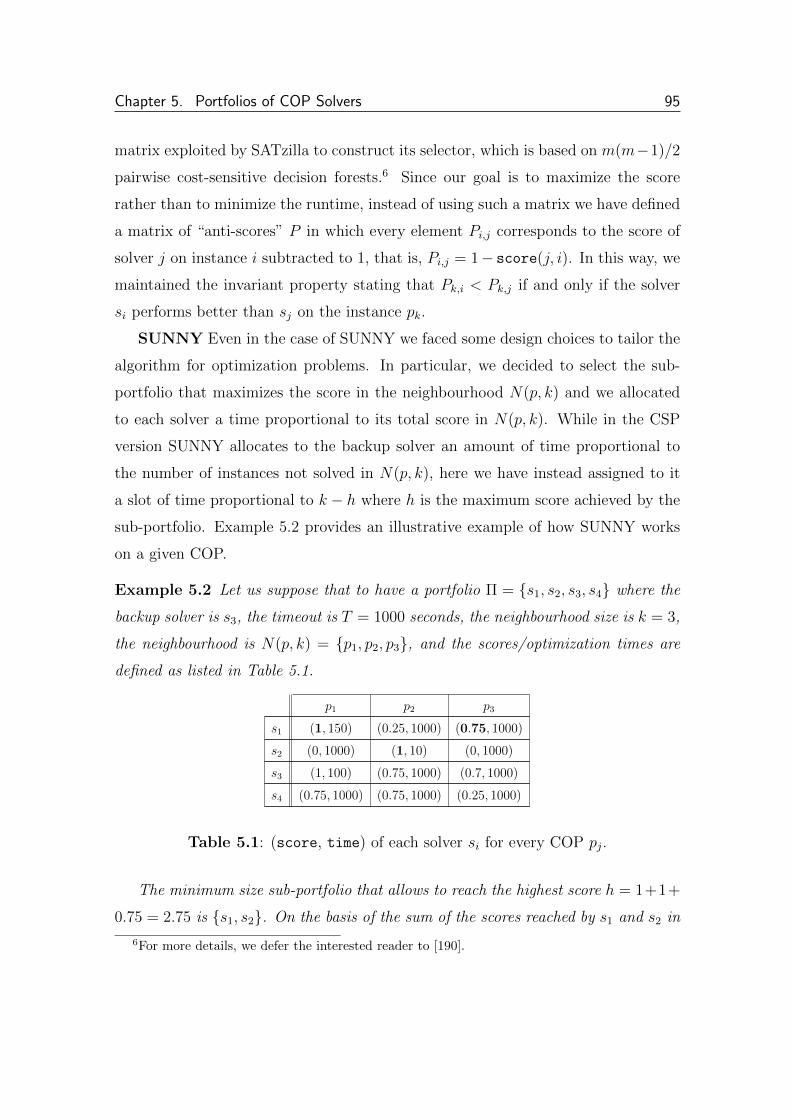
Chapter 5. Portfolios of COP Solvers 95
matrix exploited by SATzilla to construct its selector, which is based on m(m−1)/2
pairwise cost-sensitive decision forests.6 Since our goal is to maximize the score
rather than to minimize the runtime, instead of using such a matrix we have defined
a matrix of “anti-scores” P in which every element Pi,j corresponds to the score of
solver j on instance i subtracted to 1, that is, Pi,j = 1− score(j, i). In this way, we
maintained the invariant property stating that Pk,i < Pk,j if and only if the solver
si performs better than sj on the instance pk.
SUNNY Even in the case of SUNNY we faced some design choices to tailor the
algorithm for optimization problems. In particular, we decided to select the sub-
portfolio that maximizes the score in the neighbourhood N(p, k) and we allocated
to each solver a time proportional to its total score in N(p, k). While in the CSP
version SUNNY allocates to the backup solver an amount of time proportional to
the number of instances not solved in N(p, k), here we have instead assigned to it
a slot of time proportional to k − h where h is the maximum score achieved by the
sub-portfolio. Example 5.2 provides an illustrative example of how SUNNY works
on a given COP.
Example 5.2 Let us suppose that to have a portfolio Π = {s1, s2, s3, s4} where the
backup solver is s3, the timeout is T = 1000 seconds, the neighbourhood size is k = 3,
the neighbourhood is N(p, k) = {p1, p2, p3}, and the scores/optimization times are
defined as listed in Table 5.1.
p1 p2 p3
s1 (1, 150) (0.25, 1000) (0.75, 1000)
s2 (0, 1000) (1, 10) (0, 1000)
s3 (1, 100) (0.75, 1000) (0.7, 1000)
s4 (0.75, 1000) (0.75, 1000) (0.25, 1000)
Table 5.1: (score, time) of each solver si for every COP pj.
The minimum size sub-portfolio that allows to reach the highest score h = 1+1+
0.75 = 2.75 is {s1, s2}. On the basis of the sum of the scores reached by s1 and s2 in
6For more details, we defer the interested reader to [190].

96 Chapter 5. Portfolios of COP Solvers
N(p, k) (resp. 2 and 1) the slot size is t = T/(2+1+(k−h)) = 307.69 seconds. The
time assigned to s1 is 2 ∗ t = 615.38 while for s2 is 1 ∗ t = 307.69. The remaining
76.93 seconds are finally allocated to the backup solver s3. After sorting the solvers
by increasing optimization time, SUNNY executes first s2 for 615.38 seconds, then
s3 for 76.93 seconds, and finally s1 for 307.69 seconds.
The algorithm used by SUNNY on COPs is a straight generalization of the
algorithm reported in Listing 4.1 for CSPs. More precisely, in this case the func-
tion getMaxSolved(S, similar insts, KB, T) returns the maximum score achieved
by the sub-portfolio S on similar insts, instead of the number of instances of
similar insts that S is able to solve. Also the function getSubPortfolio changes
accordingly. Formally, fixed a timeout T , a portfolio Π = {s1, s2, . . . , sm}, and a
set of instances P = {p1, p2, . . . , pk}, we define an auxiliary function ψ : P(Π) →{0, 1, . . . , k} × {0, 1, . . . ,m} × [0, T ] such that, for each S ⊆ Π:
ψ(S) := (k −∑p∈P
max{score(s, p) | s ∈ S}, |S|,∑
s∈S, p∈P
time(s, p))
where |S| is the cardinality of S and score, time are defined as in Definitions 5.3
and 5.2 respectively. The function getSubPortfolio returns the subset of Π that
minimizes w.r.t. the lexicographic ordering the set of triples {ψ(S) | S ⊆ Π}.
5.1.3 Results
In this section we present the experimental results achieved by the different ap-
proaches, by using a timeout of T = 900 seconds and by varying the portfolio size in
[2, 12]. As in the previous experiments, we used a 5-fold 5-repeated cross validation
over the dataset D. To conduct the experiments we used Intel Dual-Core 2.93GHz
computers with 3 MB of CPU cache, 2 GB of RAM, and Ubuntu 12.04 Operating
System. For keeping track of the optimization times we considered the CPU time
by exploiting Unix time command. The performances are measured in terms of the
above defined metrics: score, proven, time. In addition, we also considered the
MiniZinc Challenge score as described in Section 5.1.1.

Chapter 5. Portfolios of COP Solvers 97
For ease of reading, in all the plots we report only the two best approaches
among all the off the shelf classifiers we evaluated, namely Random Forest (RF)
and SMO. As a baseline for our experiments, in addition to the Single Best Solver
(SBS) CPX, we have also introduced the Virtual Best Solver (VBS). The source
code developed to conduct and replicate the experiments is publicly available at
http://www.cs.unibo.it/~amadini/amai_2014.zip.
5.1.3.1 Score
Figure 5.2a shows the average results of score by considering all the portfolio ap-
proaches and the VBS. For the sake of readability, Figure 5.2b visualizes instead the
same results by considering the VBS, the SBS, and the two best approaches only.
As expected, all the considered approaches have good performances and greatly
outperform the SBS (even with portfolios of small size). This is encouraging, since
the portfolio composition and the portfolio approaches were defined with the aim of
maximizing the score function.
Similarly to what happens to the Percentage of Solved Instances for CSP port-
folios (see empirical results in Chapter 4), we notice that the OTS approaches have
usually lower performances, even though the gap between the best approaches and
them is not so pronounced.
The best portfolio approach is SUNNY, that reaches a peak performance of
0.8747 by using a portfolio of 10 solvers and is able to close the 90.38% of the gap
between the SBS and VBS. 3S is however very close to SUNNY, and in particular
the difference between the best performance of 3S (0.8651 with 9 solvers) and the
peak performance of SUNNY is minimal (about 0.96%).
It is interesting to notice that, unlike the others, the OTS approaches have non
monotonic performances when the portfolio sizes increases. This is particularly
evident looking at their performance decrease when a portfolio of size 7 is used
instead of one with just 6 solvers. This instability is obviously a bad property for
a portfolio approach and it is probably due to the fact that the classifiers on which
OTS approaches rely become inaccurate when they have to chose between too many
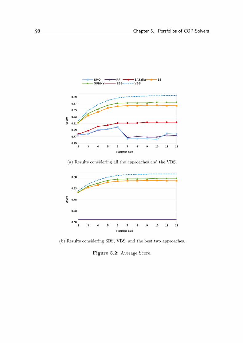
98 Chapter 5. Portfolios of COP Solvers
SMO RF SATzilla 3SSUNNY SBS VBS
2 3 4 5 6 7 8 9 10 11 120.75
0.77
0.79
0.81
0.83
0.85
0.87
0.89
Portfolio size
sc
ore
(a) Results considering all the approaches and the VBS.
2 3 4 5 6 7 8 9 10 11 120.68
0.73
0.78
0.83
0.88
Portfolio size
sc
ore
(b) Results considering SBS, VBS, and the best two approaches.
Figure 5.2: Average Score.
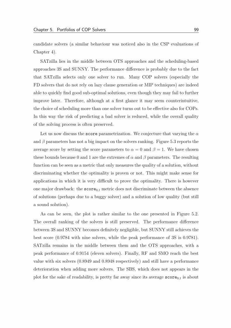
Chapter 5. Portfolios of COP Solvers 99
candidate solvers (a similar behaviour was noticed also in the CSP evaluations of
Chapter 4).
SATzilla lies in the middle between OTS approaches and the scheduling-based
approaches 3S and SUNNY. The performance difference is probably due to the fact
that SATzilla selects only one solver to run. Many COP solvers (especially the
FD solvers that do not rely on lazy clause generation or MIP techniques) are indeed
able to quickly find good sub-optimal solutions, even though they may fail to further
improve later. Therefore, although at a first glance it may seem counterintuitive,
the choice of scheduling more than one solver turns out to be effective also for COPs.
In this way the risk of predicting a bad solver is reduced, while the overall quality
of the solving process is often preserved.
Let us now discuss the score parametrization. We conjecture that varying the α
and β parameters has not a big impact on the solvers ranking. Figure 5.3 reports the
average score by setting the score parameters to α = 0 and β = 1. We have chosen
these bounds because 0 and 1 are the extremes of α and β parameters. The resulting
function can be seen as a metric that only measures the quality of a solution, without
discriminating whether the optimality is proven or not. This might make sense for
applications in which it is very difficult to prove the optimality. There is however
one major drawback: the score0,1 metric does not discriminate between the absence
of solutions (perhaps due to a buggy solver) and a solution of low quality (but still
a sound solution).
As can be seen, the plot is rather similar to the one presented in Figure 5.2.
The overall ranking of the solvers is still preserved. The performance difference
between 3S and SUNNY becomes definitely negligible, but SUNNY still achieves the
best score (0.9784 with nine solvers, while the peak performance of 3S is 0.9781).
SATzilla remains in the middle between them and the OTS approaches, with a
peak performance of 0.9154 (eleven solvers). Finally, RF and SMO reach the best
value with six solvers (0.8949 and 0.8948 respectively) and still have a performance
deterioration when adding more solvers. The SBS, which does not appears in the
plot for the sake of readability, is pretty far away since its average score0,1 is about
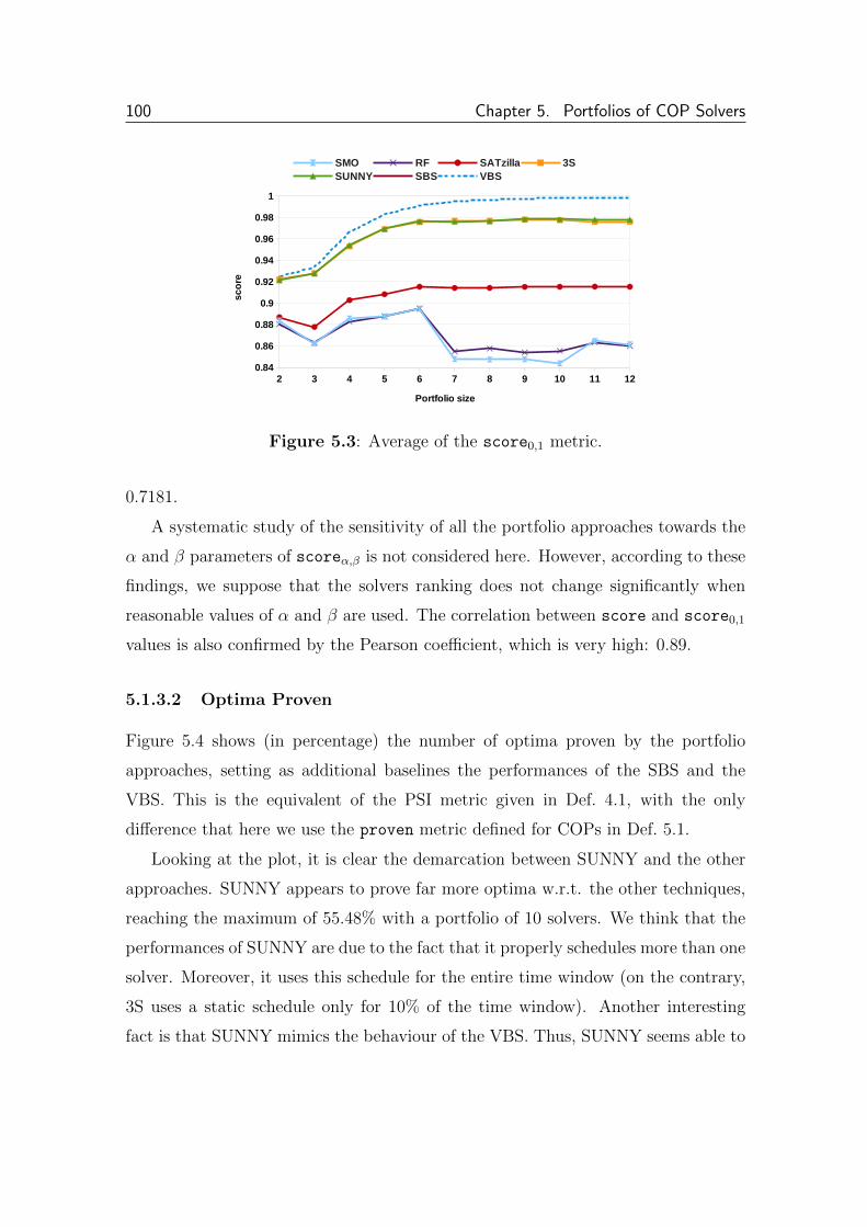
100 Chapter 5. Portfolios of COP Solvers
SMO RF SATzilla 3SSUNNY SBS VBS
2 3 4 5 6 7 8 9 10 11 120.84
0.86
0.88
0.9
0.92
0.94
0.96
0.98
1
Portfolio size
sc
ore
Figure 5.3: Average of the score0,1 metric.
0.7181.
A systematic study of the sensitivity of all the portfolio approaches towards the
α and β parameters of scoreα,β is not considered here. However, according to these
findings, we suppose that the solvers ranking does not change significantly when
reasonable values of α and β are used. The correlation between score and score0,1
values is also confirmed by the Pearson coefficient, which is very high: 0.89.
5.1.3.2 Optima Proven
Figure 5.4 shows (in percentage) the number of optima proven by the portfolio
approaches, setting as additional baselines the performances of the SBS and the
VBS. This is the equivalent of the PSI metric given in Def. 4.1, with the only
difference that here we use the proven metric defined for COPs in Def. 5.1.
Looking at the plot, it is clear the demarcation between SUNNY and the other
approaches. SUNNY appears to prove far more optima w.r.t. the other techniques,
reaching the maximum of 55.48% with a portfolio of 10 solvers. We think that the
performances of SUNNY are due to the fact that it properly schedules more than one
solver. Moreover, it uses this schedule for the entire time window (on the contrary,
3S uses a static schedule only for 10% of the time window). Another interesting
fact is that SUNNY mimics the behaviour of the VBS. Thus, SUNNY seems able to

Chapter 5. Portfolios of COP Solvers 101
SMO RF SATzilla 3SSUNNY SBS VBS
2 3 4 5 6 7 8 9 10 11 1240
42
44
46
48
50
52
54
56
58
60
Portfolio size
pro
ve
n [
%]
Figure 5.4: Percentage of Optima Proven.
properly exploit the addition of a new solver by taking advantage of its contribution
in terms of proven.
The closest approach to SUNNY is 3S, which reaches a maximum of 51.51%
with 10 solvers. The other approaches —that selects just one solver per instance—
appear to be worse than SUNNY and 3S, and fairly close to each other. Moreover,
it is evident that all the portfolio approaches greatly outperform the SBS. SUNNY
in particular is able to close the 82.78% of the gap between the SBS and VBS.
It is interesting to notice that proven is actually not so dissimilar from score:
the Pearson coefficient is about 0.72. A possible explanation is that the proven
function is actually equivalent to the score0,0 function.
5.1.3.3 Optimization Time
Figure 5.5 presents the average optimization times of the various approaches, setting
as additional baselines the performances of the SBS and the VBS. It is easy to note
that this metric is the equivalent of the the AST metric given in Def. 4.2 for CSPs.
Clearly, here we use the time metric defined for COPs in Def. 5.2.
Even in this case, the results turn out to be related to those previously reported.
The only remarkable difference concerns the 3S approach, that here does not perform
as well as before. We think that this is due to the fact that 3S is a portfolio

102 Chapter 5. Portfolios of COP Solvers
SMO RF SATzilla 3SSUNNY SBS VBS
2 3 4 5 6 7 8 9 10 11 12400
420
440
460
480
500
520
540
560
Portfolio size
tim
e [
se
c.]
Figure 5.5: Average Optimization Time.
that schedules more than one solver and it does not explicitly employ heuristics to
decide which solver has to be executed first. SUNNY instead does not suffer from
this problem since it schedules the solvers according to their performances on the
already known instances. However, the performances of 3S look very close to those
of SATzilla and the OTS approaches.
Even in this case we can observe the good performance of SUNNY that is able
to close the 81.55% of the gap between SBS and VBS reaching a peak performance
of 428.95 seconds with a portfolio of 12 solvers. The second position is this time
achieved by SMO, that with 12 solvers reaches a minimum of 471.05 seconds.
As one can expect, time is by definition strongly anti-correlated to score (the
Pearson coefficient is −0.88) and however moderately related also to the score
metric (the Pearson coefficient is −0.63).
5.1.3.4 MiniZinc Challenge Score
In this section we present the results obtained by considering the scoring metric of
the MiniZinc Challenge, hereafter abbreviated as MZCS (MiniZinc Challenge Score).
Given the nature of MZCS (see Section 5.1.1) it makes no sense to introduce the
VBS. In fact, due to the Borda comparisons, this addition would only cause a lower-
ing of the scores of the other “real” solvers. Conversely, it is certainly reasonable to

Chapter 5. Portfolios of COP Solvers 103
consider the SBS against the portfolio solvers. In Figure 5.6 is depicted the average
score achieved by every portfolio approach and the SBS.
SBS 3S RF
SATzilla SMO SUNNY
2 3 4 5 6 7 8 9 10 11 121.5
2
2.5
3
3.5
4
Portfolio size
MZ
CS
Figure 5.6: MiniZinc Challenge Score.
It interesting to note that the results are somehow different from what observed
using other evaluation metrics. Even if SUNNY is still the best approach, we notice
a remarkable improvement of SATzilla as a well as a significant worsening of 3S, that
turns out to be always worse than the SBS. We think that this is due to the fact that
SATzilla is able to select solvers that give better answers w.r.t. the OTS approaches
(especially when optimality is not proven) and that, in case of indistinguishable
answers, the scheduling-based approach of 3S is penalized by the Borda count used
in the MiniZinc Challenge.
Note that, due to the pairwise comparisons between the solvers, the performance
of the SBS is not constant. Indeed, its performance depends on the performance of
the other solvers of the portfolio. The better a solver becomes, the more solvers it
is able to beat, thus improving its score. Moreover, differently from score, here the
score is not between 0 and 1 since MZCS is a value in the range [0,m− 1] where m
is the number of the solvers involved in the Borda count. The peak performance is
achieved by SUNNY that with 6 solvers has an average score of 3.77, meaning that
on average it is able to beat almost 4 out of 5 competitors per instance. All the other
approaches reach instead the peak performance with 2 solvers, in correspondence

104 Chapter 5. Portfolios of COP Solvers
with the worst SUNNY performance.
The different nature of the MZCS metric w.r.t. the other metrics is also under-
lined by the very low correlation. In particular, there is in practice no correlation
with proven (0.31) and time (−0.07). More pronounced, but still rather low, the
correlation between MZCS and score: about 0.53.
5.1.3.5 Summary
We tackled the problem of developing portfolio approaches for solving COPs. Firstly,
we introduced a function score which takes into account the quality of the solvers
solutions. Then, we used such a metric (and others) for simulating and comparing
different portfolio techniques properly adapted to the COP world.
The results obtained clearly indicate that, even in the optimization setting, the
portfolio approaches have remarkable better performances than a single solver. We
observed that, when trying to prove optimality, the number of times a solver cannot
complete the search is not negligible. Moreover, the optimization times have a
heavy-tailed distribution typical of complete search methods [85]. Hence, a COP
setting can be considered an ideal scenario to apply portfolio approaches and obtain
statistically better solvers by exploiting existing ones [84].
We noticed that, even though at a first glance it can seem counterintuitive,
the best performances were obtained by SUNNY. This strategy reduces the risk of
choosing the wrong solver and, apparently, this is more important than performing
part of the computation again, as could happen when two (or more) solvers are run
on the same instance.
It is important to emphasize that the results reported in this section can be
considered as a “lower bound”. Indeed, as done in the experiments of Chapter 4,
we did not actually execute each portfolio solver but we simulated its outcome by
exploiting the information already computed. This is certainly useful for avoiding
the enormous effort of running every portfolio solver on each fold/repetition. How-
ever, as formerly stressed, the estimations reported in this section just consider each
Chapter 5. Portfolios of COP Solvers 105
constituent solver individually, without taking into account the potential use of “co-
operative strategies” among the constituent solvers. In the next section we see a
possible way to leverage the collaboration between different COP solvers.
5.2 Sequential Time Splitting and Bound Com-
munication
As seen so far, scheduling a subset of the constituent solvers of a given portfolio
seems to be a good strategy (see for instance the performance of SUNNY, but also
[113, 92, 16, 160, 151]) . Since often the solving time of hard combinatorial problems
is either relatively short or very long, the scheduling approach naturally handles the
heavy tailed nature of solving.
In particular, in a COP setting a solver can transmit useful bounds information
to another one if they are scheduled sequentially. In a portfolio scenario, a partial
solution found by a solver s1 is indeed a token of knowledge that s1 can pass to
another solver s2 in order to prune its search space and therefore possibly improve its
solving process. In this section we thus address the problem of boosting optimization
by exploiting the sequential cooperation of different COP solvers. To do so, we
will introduce the notion of solving behaviour for taking into account the anytime
performance of the solvers.
This section basically reports the work we presented in [12].
5.2.1 Solving Behaviour and Timesplit Solvers
Let us fix a dataset D of COPs, a set S of COP solvers, and a solving timeout T .
We wish to determine the best sequence of solvers in S to run on p and for how long
to run each solver within [0, T ] in order obtain the best result for instance p. Ideally
we aim to improve the best solver of S for the instance p. To do so, we introduce
the concept of solving behaviour.

106 Chapter 5. Portfolios of COP Solvers
Definition 5.4 (Behaviour) Let us fix a dataset D of COPs, a set S of COP
solvers, and a solving timeout T . We define the (solving) behaviour B(s, p) of a
solver s ∈ S applied to a problem p ∈ D over time [0, T ] as an ordered sequence of
pairs B(s, p) := [(t1, v1), (t2, v2), . . . , (tn, vn)] such that:
• B(s, p) ⊆ [0, T )× R;
• ti is the time when s finds a solution (i = 1, 2, . . . , n);
• vi = val(s, p, ti) is the objective value of such a solution (i = 1, 2, . . . , n).
We can consider the pairs ordered so that t1 < t2 < · · · < tn while v1 > v2 > · · · > vn
since we assume the solving process is monotonic.
For example, consider the behaviours B(s1, p) = [(10, 40), (50, 25), (100, 15)] and
B(s2, p) = [(800, 45), (900, 10)] illustrated in Figure 5.7a with a timeout of T = 1000
seconds. The best value v∗ = 10 is found by s2 after 900 seconds, but it takes 800
seconds to find its first solution (v = 45). Meanwhile, s1 finds a better value (v = 40)
after just 10 seconds and even better values in just 100 seconds. So, the question is:
what happens if we “inject” the upper bound 40 from s1 to s2? Considering that
starting from v = 45 the solver s2 is able to find v∗ in 100 seconds (from 800 to
900), hopefully starting from any better (or equal) value v′ ≤ 45 the time needed
by s2 to find v∗ is no more than 100 seconds. Note that from a graphical point of
view what we would like to do is therefore to “shift” the curve of s2 towards the
left from t = 800 to 10, by exploiting the fact that after 10 seconds s1 can suggest
to s2 the upper bound v = 40. The cooperation between s1 and s2 would thereby
reduce by ∆t = 790 seconds the time needed to find v∗, and moreover would allow
us to exploit the remaining ∆t seconds for finding better solutions or even proving
the optimality of v∗. However, note that the virtual behaviour may not occur: it
may be that s2 calculates important information in the first 800 seconds required to
find the solution v∗ = 10, and therefore the injection of v = 40 could be useless (if
not harmful).

Chapter 5. Portfolios of COP Solvers 107
10 50 100 800 900 1000Time [seconds]
10
15
25
40
45
Solu
tion
Valu
e
∆t
s2
s1
(a) σ = [(s1, 10), (s2, 990)]
100 250 500 700 800 900 1000Time [seconds]
100
75
50
30
20
10
Solu
tion
Valu
es2
s1
(b) σ = [(s2, 1000)]
20 100 250 400 600 800 1000Time [seconds]
100
80
60
50
30
20
10
Solu
tion
Valu
e ∆1
∆2s1
s2
s3
(c) σ = [(s2, 100), (s3, 150), (s1, 750)]
20 100 250 400 600 800 1000Time [seconds]
100
80
60
50
30
20
10
Solu
tion
Valu
e
∆1
∆2s1
s2
(d) σ = [(s1, 100), (s2, 150), (s3, 750)]
Figure 5.7: Examples of solving behaviours and corresponding time splitting σ.

108 Chapter 5. Portfolios of COP Solvers
Definition 5.5 (Timesplit Solver) Given a problem p ∈ D and a schedule of
solvers σ := [(s1, t1), (s2, t2), . . . , (sk, tk)] ⊆ S × [0, T ) we define the corresponding
timesplit solver as a particular solver that:
(i) first, runs s1 on p for t1 seconds;
(ii) then, for i = 1, 2, . . . , k− 1, runs si+1 on p for ti+1 seconds possibly exploiting
the best solution found by the previous solver si in ti seconds.
The base of the timesplit solver σ is a timesplit solver σ where we omit the last
solver in the schedule: σ := [(s1, t1), (s2, t2), . . . , (sk−1, tk−1)].
We can see a timesplit solver as a “compound solver” that not only schedules the
solvers s1, s2, . . . , sm but also exploits their sequential cooperation. The base σ of a
timesplit solver σ is itself a timesplit solver that ideally contributes to improve the
last scheduled solver sk. Note that, for simplicity, we will use the same notation
to denote a timesplit solver and its corresponding schedule. As an example, in
Figure 5.7a the ideal timesplit solver would be defined by σ = [(s1, 10), (s2, 990)],
while σ = [(s1, 10)]. There are however cases in which the timesplit solver is actually
a single solver, since the best solver is not virtually improvable by any other. This
happens when every solution found by the best solver is also the best solution found
so far (e.g., see Figure 5.7b). Moreover, there may be also cases in which splitting
the time window in more than two slots (even alternating the same solvers) may
ideally lead to better performances. Indeed, the “overall” best solver at the time
edge T might no longer be the best one at a previous time t < T . For example, in
Figure 5.7c the best solver at time t ≥ 800 is s1, at time 400 ≤ t < 800 is s3 while
for t ≤ 400 is s2; in Figure 5.7d the best solver is s1 if t < 400 or t ≥ 800, while for
400 ≤ t < 800 is s2.
5.2.2 Splitting Selection and Evaluation
Once informally hypothesized the potential benefits of timesplit solvers, some ques-
tions naturally arise:

Chapter 5. Portfolios of COP Solvers 109
• First, which metric(s) is reasonable to formally define the “best solver”?
• Furthermore, how do we split the time window between solvers for determining
the (virtually) best timesplit solver?
• Finally, to what extent do timesplit solvers act like the virtual timesplit
solvers?
In order to answer these questions we fixed some proper metrics, defined a splitting
algorithm and empirically evaluated the assumptions previously introduced.
5.2.2.1 Evaluation Metrics
In order to evaluate the performances of different COP solvers (and thus formally
define the notion of best solver) we examine a number of metrics for grading a solver
s on a problem p over a time limit T .
In addition to the proven, time, and score metric introduced above (see Def.
5.1, 5.2, 5.3 respectively) here we introduce a new metric able to estimate the any-
time solver performance.
Definition 5.6 (area) Let us fix a dataset of COPs D, a set of COP solvers S,
and a solving timeout T . Given a problem p ∈ D, let Wp := {val(s, p, t) | s ∈S, t ∈ [0, T ]} be the set of all the solutions of p found by any solver at any time. If
B(s, p) = [(t1, v1), (t2, v2), . . . , (tn, vn)] is the behaviour of solver s on problem p, we
define the (solving) area of s on p as a function area : S× D→ [0, T ] such that:
area(s, p) := t1 +n∑i=1
(0.25 + 0.5 · val(s, p, ti)−minWp
maxWp −minWp
)(ti+1 − ti)
where tn+1 := time(s, p).
As the name implies, area is a normalized measure of the area under a solver
behaviour. Actually the solving area could be seen as the cumulative sum of the
anytime score of a solver in the solving time window. The main difference is that the
score function scales the objective values in the range [minVp,maxVp], where Vp =
110 Chapter 5. Portfolios of COP Solvers
{val(s, p, T ) : s ∈ S} is the set of the objective function values found by any solver
s at the time limit T . Conversely, area uses instead the range [minWp,maxWp] for
mapping all the solutions found by any solver at any time. Without this change, the
partial solutions found at time t < T might not be adequately addressed. Similarly
to scoreα,β, even the area metric may be defined in terms of α, β parameters:
areaα,β(s, p) = t1 +n∑i=1
(α + (β − α) · val(s, p, ti)−minWp
maxWp −minWp
)(ti+1 − ti)
However, as for the score, we assume α = 0.25 and β = 0.75.
Example 5.3 Consider the behaviours of the solvers s1, s2, s3 on a minimization
problem p shown in Example 5.1 on page 91. Precisely, the behaviours are:
• B(s1, p) = [(100, 70), (200, 60), (500, 40)];
• B(s2, p) = [(400, 50)];
• B(s3, p) = [(550, 30), (650, 20), (700, 10)].
The optimization times are instead time(s1, p) = time(s2, p) = T = 1000 while
time(s3, p) = 900. The set of the anytime values is Wp = {10, 20, 30, 40, 50, 60, 70}.The scaling of such values in [0.25, 0.75] produces the corresponding normalized val-
ues W p = {0.25+0.5· v−1060
: v ∈ Wp} = {0.25, 0.33, 0.42, 0.5, 0.58, 0.67, 0.75}. Figure
5.8 depicts the “normalized” behaviours of such solvers, where instead of the original
objective values of Wp we show the corresponding normalized values of W p.
The area of s1 is area(s1, p) = 100 + 0.75 · (200− 100) + 0.67 · (500− 200) + 0.5 ·(1000− 500) = 626. The area of s2 is area(s2, p) = 400 + 0.58 · (1000− 400) = 748
while area(s3, p) = 550+0.42·(650−550)+0.33·(700−650)+0.25·(900−700) = 658.5.
Note that even if s3 finds the optimal value v∗ = 10, and proves its optimality, its
area is worse than that of s1 (even if the best value found by s1 is 40, which is
worse than the worst value found by s3). This is because area rewards more a solver
that quickly finds good solutions rather than one that slowly finds the best solutions
(maybe by also proving the optimality).

Chapter 5. Portfolios of COP Solvers 111
0 100 200 400 500550 650700 900 1000
Time [seconds]
0.00
0.75
0.67
0.58
0.50
0.42
0.33
0.25
1.00
Solu
tion V
alu
e
s1
s2
s3
Figure 5.8: Solving area of s1, s2, s3.
The solving area is similar to the primal integral [27] used for measuring impact of
heuristics for MIP solvers, but differs since the primal integral assumes the optimal
solution is known, while area also differentiates between finding and proving a
solution optimal. The area metric folds in a number of measures the strength of
an optimization algorithm: the quality of the best solution found, how quickly any
solution is found, whether optimality is proven, and how quickly good solutions are
found. Even though the ideal goal is to find the best objective value and hopefully
proving its optimality, area allows us to discriminate much more between solvers,
since we capture the trade-off between speed and solution quality. Two solvers
which eventually reach the same best solution (without proving optimality) are
indistinguishable with the other measures, but we would almost certainly prefer the
solver that finds the solution(s) faster. Furthermore, consider two solvers that prove
optimality at the same instant t < T : while both will have time = t, area will
reward the solver in [0, t] that finds better solutions faster.
Finally, we can now define the best solver of S for a given problem p as the
solver s ∈ S which minimizes (w.r.t. the lexicographic ordering) the set of triples
(1 − score(s, p), time(s, p), area(s, p)). Intuitively, the best solver is the one that

112 Chapter 5. Portfolios of COP Solvers
finds the best solution within the time limit T , breaking ties by using minimum
optimization time first, and then minimum area (i.e., giving priority to the solvers
that prove optimality in less time, or at least that quickly find sub-optimal solutions).
Note that it is not unlikely that two different solvers s1 and s2 have the same value
of score and time. For example, consider a problem p for which after T seconds s1
and s2 find the same objective value v without proving its optimality. By definition,
score(s1, p) = score(s2, p) and time(s1, p) = time(s2, p) = T . Hence, the best
solver between s1 and s2 will be the one with lower area.
5.2.2.2 TimeSplit Algorithm
Our goal is now to find a suitable timesplit solver for instance p which can improve
upon the best solver for p. The algorithm TimeSplit described with pseudo-code in
Listing 5.1 encodes what was informally explained earlier (see Figure 5.7). Given as
input a problem p, a portfolio Π ⊆ S, and the timeout T , the basic idea of TimeSplit
is to start from the behaviour of the best solver s2 ∈ Π for p and then examine other
solvers behaviours looking for the maximum ideal “left shift” toward another solver
s1 ∈ Π \ {s2}. Then, starting from s1, this process is iteratively repeated until no
other shift is found. The best solver of Π is assigned to s2 via function best solver
in line 2, while line 3 sets the current schedule σ to [(s2, T )]. In line 4 auxiliary
variables are initialized: tot shift keeps track of the sum of all the shifts identified,
max shift is the current maximum shift that s2 can perform, split time is the time
instant from which s2 will start its execution, while split solver is the solver that has
to be run before s2 until split time instant. The while loop enclosed in lines 5-18
is repeated until no more shifts are possible (i.e., max shift = 0). The three nested
loops starting at lines 7-9 find two pairs (t1, v1) and (t2, v2) such that s2 can virtually
shift to another solver s1, i.e., such that in the current solving window [0, split time]
we have that at time t1 < t2 solver s1 finds a value v1 better than or equal to v2. If
the actual shift ∆t = t2 − t1 is greater than max shift , in lines 11-13 the auxiliary
variables are updated accordingly. In line 15, the allocated time of the current first
solver of σ (i.e., s2) is decreased by an amount of time max shift + split time (note

Chapter 5. Portfolios of COP Solvers 113
that first(σ) is a reference to the first element of σ, while snd returns the second
element of a pair, i.e. the allocated time in this case). This is because split time
seconds will be allocated to split solver (line 16: push front inserts an element
on top of the list) while max shift seconds corresponding to the ideal shift will be
later donated to the ’overall’ best solver of Π (i.e., the last solver of σ) via tot shift
variable.
1 TimeSplit(p,Π, T ) :
2 s2 = best solver(p,Π, T )
3 σ = [(s2, T )]
4 tot shift = 0 ; max shift = 1 ; split time = T ; split solver = s2
5 while max shift > 0 :
6 max shift = 0
7 for (t2, v2) in {(t, v) ∈ B(s2, p) | t ≤ split time} :
8 for s1 in Π \ {s2} :
9 for (t1, v1) in {(t, v) ∈ B(s1, p) | t < t2 ∧ v ≤ v2} :
10 if t2 − t1 > max shift :
11 max shift = t2 − t112 split time = t1
13 split solver = s1
14 if max shift > 0 :
15 first(σ).snd −= max shift + split time
16 push front(σ, (split solver , split time))
17 tot shift += max shift
18 s2 = split solver
19 last(σ).snd += tot shift
20 return σ
Listing 5.1: TimeSplit Algorithm.
At this stage, the search for a new shift is restricted to the time interval [0, split time]
in which the new best solver s2 will be split solver (line 18). Once out of the while
loop (no more shifts are possible) the total amount of all the shifts found is added
to the best solver (line 19: last(σ) is a reference to the last element of σ) and the
final schedule is finally returned in line 20.

114 Chapter 5. Portfolios of COP Solvers
5.2.2.3 TimeSplit Evaluation
In order to experimentally verify the correctness of our assumptions on the behaviour
of timesplit solvers, we tested TimeSplit by considering a portfolio Π constructed
from the solvers of the MiniZinc 1.6 suite (i.e., CPX, G12/FD, G12/LazyFD, and
G12/MIP) with some additional solvers disparate in their nature, namely: Ge-
code [73] (CP solver), MinisatID [50] (SAT-based solver), Chuffed (CP solver with
Lazy Clause Generation), and G12/Gurobi (MIP solver). We retrieved and filtered
an initial dataset D of 4864 MiniZinc COPs from MiniZinc 1.6 benchmarks and the
MiniZinc Challenges 2012/13 and then ran TimeSplit using a solving timeout of
T = 1800 seconds. In particular, we ran and compared two versions of the algorithm:
the original one and a variant (denoted TS-2 in what follows) in which we imposed
a maximum size of 2 solvers for each schedule σ. This is because splitting [0, T ]
in too many slots can be counterproductive in practice: excessive fragmentation of
the time window may produce time slots that are too short to be useful. Once
executed these algorithms, in order to evaluate their significance we discarded all
the “degenerate” instances for which the potential total shift was minimal (less than
5 seconds). We then ended up with a reduced dataset D′ ⊂ D of 596 instances. We
ran timesplit solvers defined by the schedule returned by each algorithm on every
instance of D′. In addition, we added as a baseline the Virtual Best Solver (VBS).
Finally, we evaluated and compared the average performance in terms of the above
mentioned metrics: score, proven, time, area.
Table 5.2 shows the average results for each approach. As can be seen, the
performances are rather close. On average, VBS is still the best solver if we focus on
score metric (i.e., considering only the values found at the time limit T ). Regarding
proven and time metrics, we can observe a substantial equivalence: VBS is slightly
better in terms of percentage of optima proven, while it is worse than TimeSplit and
TS-2 if we consider the average time to prove optimality. Conversely, looking at area
the situation appears to be more clearly defined: on average, VBS is substantially
worse than both TimeSplit and TS-2. This means that, even if the virtual behaviour
does not always occur, often the time splitting we propose is able to find good partial

Chapter 5. Portfolios of COP Solvers 115
solutions more quickly than the best solver of Π. Focusing just on the two versions
of TimeSplit, we can also note that these are substantially equivalent: this confirms
the hypothesis that limiting the algorithm to schedule only two solvers is a reasonable
choice (TS-2 seems slightly better than TimeSplit on average). Indeed, among all
the instances of D′, only for 53 of them TimeSplit has produced a schedule with
more than two solvers. Table 5.3 shows instead how many times the approach on
the i-th row is better than the one on the j-th column. In this case we can note
that TimeSplit and TS-2 perform better than VBS: indeed, in the cases in which
the score is the same for both the approaches, often the timesplit solvers take less
time to find a (optimal) solution.
score proven time area
VBS 82.40% 34.73% 1298.67 478.05
TimeSplit 80.49% 33.67% 1263.74 347.91
TS-2 80.60% 33.89% 1259.98 343.97
Table 5.2: Average performances.
VBS TimeSplit TS-2
VBS — 222 232
TimeSplit 373 — 40
TS-2 364 13 —
Table 5.3: Pairwise Comparisons.
Note that for 375 problems (62.92% of D′) at least one between TimeSplit and
TS-2 is better than the VBS, i.e., the best solver of {TimeSplit, TS-2,VBS} is
TimeSplit or TS-2. Let D∗ be the set of such instances, and considering the base
σ(p) of each schedule σ(p) returned by the best approach between TimeSplit and
TS-2 for each instance of p ∈ D∗, we noticed an interesting fact: the time allocated
to σ(p) is usually pretty low. Figure 5.9 reports the distribution of such each times.
As can be seen, almost all the times are concentrated in the lower part of the graph:

116 Chapter 5. Portfolios of COP Solvers
even if the maximum value is 1363 seconds, the mean is less than a minute (54.18
seconds to be precise) while the median value is significantly lower (9 seconds).
0
200
400
600
800
1,000
1,200
1,400
Times Mean (Times)
Instances
Tim
e [
se
c.]
Figure 5.9: Times allocated to σ(p) for each p ∈ D∗.
Figure 5.10 shows an example of the benefits of timesplit solvers on an instance
of the Resource-Constrained Project Scheduling Problem (RCPSP) [34] taken from
the MiniZinc suite.7 The timesplit solver runs the schedule [(CPX, 1), (MinisatID,
1799)] since after just one second CPX is able to find the value 101. The point is
that CPX never improves that value in the remaining 1799 seconds. Conversely,
MinisatID is slower in finding good solutions (it finds 101 at time 799) but in the
end it finds a better value than CPX (i.e., 100 at time 844). From Figure 5.10 we
can see that —by receiving the bound 101 from CPX after 1 second— MinisatID
is able to find the value 100 in just 173 seconds. Moreover, it finds the value 99 at
time 191 and at time 217 it proves that 98 is an optimal value.
5.2.3 Timesplit Portfolio Solvers
The results of Section 5.2.2.3 show that in a non-negligible number of cases the
benefits of using a timesplit solver are tangible. Unfortunately, in such experiments
for every instance we already knew the corresponding runtimes of each solver of
the portfolio. What we want is instead to predict and run the best timesplit solver
for a new unseen instance. Regrettably, given runtime prediction of a solver is a
non-trivial task, predicting the detailed solver behaviour on a new test instance is
7 Precisely, the model is in minizinc-1.6/benchmarks/rcpsp/rcpsp.mzn while the corre-
sponding data is in minizinc-1.6/benchmarks/rcpsp/data_psplib/j120/J120_9_6.dzn

Chapter 5. Portfolios of COP Solvers 117
1 217 844 1800Time [seconds]
98
99
100
101
Obje
ctiv
e V
alu
e
CPX
MinisatID
[(CPX, 1), (MinisatID, 1799)]
Figure 5.10: Splitting benefits on a RCPSP instance.
even harder. Indeed, in our case we can not simply limit ourselves to guess the
best solver for a new instance, but we should instead predict a suitable timesplit
solver [(s1, t1), (s2, t2), . . . , (sk, tk)]. Moreover, even if in most cases the TimeSplit
algorithm works pretty well, on the others we noticed a considerable number of
instances for which this algorithm is ineffective (or even harmful). Therefore, a
successful strategy should be able not only to predict a proper timesplit solver,
but also to distinguish between the instances for which the timesplit is actually
useful and those where it is counterproductive. Furthermore, another interesting
observation that has emerged from the results of Section 5.2.2.3 is that often for
the “significant” timesplit solvers is sufficient to run the base of the schedule for a
relatively low number of seconds in order to allow an effective improvement of the
best solver.
On the basis of these observations and motivations, we propose a generic and
hybrid framework that we called Timesplit Portfolio Solver.
Definition 5.7 (Timesplit Portfolio Solver) Let p ∈ D be a COP and T a solv-
ing timeout. A Timesplit Portfolio Solver (TPS) is a timesplit solver defined
as:
TPS(p) := [(S, C), (D(p), T − C)]

118 Chapter 5. Portfolios of COP Solvers
where:
• (S, C) is a static timesplit solver, pre-computed off-line, that will run for the
first C < T seconds;
• (D(p), T − C) is a dynamic timesplit solver, computed on-line by a given
prediction algorithm D(p), that will run for the remaining T − C seconds.
The underlying idea of TPS is to exploit for the first C seconds a fixed schedule
calculated a priori, whose purpose is to produce as many good sub-optimal solutions
as possible. If after C seconds the optimality is still not proven, in the remaining
T−C seconds the algorithm D(p) tries to predict which is the best (timesplit) solver
for p that will be executed taking advantage of any upper bound provided by S.
Since TPS is a general model that can be arbitrarily specialized, in the rest of
this section we explain in more detail what choices we made and what algorithms
we used to define and evaluate (variants of) TPS.
5.2.3.1 Static Splitting
Drawing inspiration from what was done in [113] for SAT problems, we decided
to compute a static schedule of solvers according to the outcomes of TimeSplit
on a given set of training instances. While in [113] the authors solve a Resource
Constrained Set Covering Problem (RCSCP) in order to get a schedule that max-
imizes the number of training instances that can be solved within a time limit of
C = T/10 seconds, in our case the objective is different. What we would like is
indeed to compute a schedule that may act as a good base for the solver(s) who will
be executed in the remaining T −C seconds. To do this, we first identify by means
of TimeSplit algorithm the set D∗ of all the training instances for which a timesplit
solver outperforms the VBS.
Let σ(p) = [(sp,1, tp,1), (sp,2, tp,2), . . . , (sp,k, tp,k)] be the schedule returned by the
TimeSplit algorithm on each p ∈ D∗. We look for a schedule S that maximizes
the number of time slots tp,i ∈ σ(p) for i = 1, 2, . . . , k − 1 that are covered, that is
the portfolio solver allocates at least tp,i seconds to solver sp,i. Again, note that we
Chapter 5. Portfolios of COP Solvers 119
consider the base σ(p) instead of σ(p) since at this stage we are not interested in
choosing the best solver: we want to determine an effective timesplit solver able to
quickly find suitable sub-optimal solutions. However, a nice side-effect of this ap-
proach is that it also may be able to solve quickly those instances that are extremely
difficult for some solvers but very easy for others.
For each p ∈ D∗, we define ∇p ⊆ S× [0, C] as the set:
∇p = {(sp,i, t) | (sp,i, tp,i) ∈ σ(p), tp,i ≤ t ≤ C}
of all the pairs (sp,i, t) that cover the time slot tp,i within C seconds. Named
Π∗ =⋃p∈D∗{s ∈ Π : (s, t) ∈ ∇p}
the set of the solvers of a portfolio Π ⊆ S that appear in at least a ∇p, and fixed
C = T/10, we solve the following Set Covering problem:
min
(C + 1)∑p∈D∗
yp +∑s∈Π∗
∑t∈[0,C]
t xs,t
s.t.
yp +∑
(s,t)∈∇p
xs,t ≥ 1 ∀p ∈ D∗
∑t∈[0,C]
xs,t ≤ 1 ∀s ∈ Π∗
∑s∈Π∗
∑t∈[0,C]
t xs,t ≤ C
yp, xs,t ∈ {0, 1} ∀p ∈ D∗, ∀s ∈ Π∗, ∀t ∈ [0, C]
For each pair (s, t) there is a binary variable xs,t that will be equal to one if and only
if in S the solver s will run for t seconds. For each problem p, the binary variable
yp will be one if and only if S cannot cover any time slot of σ(p). Constraint
yp +∑xs,t ≥ 1 imposes that instance p is covered (possibly setting yp = 1 in the
worst case) while∑t xs,t ≤ C ensures that S will not exceed the time limit C. The
objective is thus to minimize the number of uncovered instances first (by means of
C + 1 coefficient for each yp), and the total time of S then (using the t coefficient
for each xs,t).

120 Chapter 5. Portfolios of COP Solvers
Note that the solution of the problem defines an allocation ξ = {(s, t) : xs,t = 1}and not actually a schedule: we still have to define the execution order of the
solvers. Since the interaction between different solvers is not easily predictable, and
neither generalizable, we decided to use a simple and reasonable heuristic: we get
the schedule S by sorting each (s, t) ∈ ξ by increasing allocated time t.
5.2.3.2 Dynamic Splitting
Once defined the static part of TPS, we want to determine an algorithm D(p) able
to predict for a new unseen instance p a proper (timesplit) solver to run for T − Cseconds after [(S, C)]. Inspired by the results already presented in Section 4.2.3 and
5.1.3 we made use of the SUNNY algorithm.
The reasons behind the choice of SUNNY are essentially two. First, even if
originally designed for CSP portfolios, SUNNY turns out to perform well also on
COPs. Second, SUNNY is not limited to predict a single solver but selects instead
a schedule of solvers: in other terms, it implicitly returns a timesplit solver (e.g.,
see Example 5.2).
5.2.4 Empirical Evaluation
In order to measure the performances of the TPS instance described in Sections
5.2.3.1 and 5.2.3.2, in the following referred to as sunny-tps, we considered a solving
timeout of T = 1800 seconds, a threshold of C = T/10 = 180 seconds for the static
schedule, the portfolio Π = {Chuffed, CPX, G12/FD, G12/LazyFD, G12/Gurobi,
G12/MIP, Gecode, MinisatID} and the dataset D of 4864 MiniZinc instances men-
tioned in Section 5.2.2.3.
We evaluated all the approaches by using a 10-fold cross validation [15]. D was
randomly partitioned in 10 disjoint folds D1,D2, . . . ,D10 treating in turn one fold Di
as the test set TSi (i = 1, 2, . . . , 10) and the union of the remaining folds⋃j 6=iDj as
the training set TRi. For each training set TRi we then computed a corresponding
static schedule (Si, 180) as explained in Section 5.2.3.1, and for every instance p ∈

Chapter 5. Portfolios of COP Solvers 121
TSi we computed and executed the timesplit solver [(Si, 180), (Di(p), 1620)] where
Di(p) is the schedule returned by SUNNY algorithm for problem p using a reduced
solving window of T − C = 1620 seconds.8 Contrary to what has been done in
the previous experiments (see Sections 4.1.2, 4.2.3, and 5.1.3) we did not use a 5-
repeated 5-fold cross validation. This was essentially done for reducing the effort of
running every approach for 4864 · 5 = 24320 times. Indeed, it is worth nothing that
while in Sections 4.1, 4.2, 5.1 the portfolio evaluation was based on simulations of
the approaches according to the already computed behaviours of every solver of Π
on every instance of D, in this work all the approaches have been actually run and
evaluated. Indeed, as shown also in Section 5.2.2.3, in this case we can not make
use of simulations since the side effects of bounds communication are unpredictable
in advance.
For computing Di(p) the SUNNY algorithm has to retrieve the k instances of
TRi closest to p. In order to do so, a proper set of features has to be extracted from p
(and each instance of TRi). Instead of using the whole set of 155 features extracted
by the mzn2feat tool described in 4.2.2.3) we decided to select a proper subset of
them by exploiting the new extractor mzn2feat-1.0.9 This tool is a new version
of mzn2feat designed to be more portable, light-weight, flexible, and independent
from the particular machine on which it is run as well as from the specific global
redefinitions of a given solver. Indeed, mzn2feat-1.0 does not compute features
based on graph measures (since this process could be very time/space consuming),
solver specific features (like global constraint redefinitions) and dynamic features (to
decouple the extractor from a particular solver and from the given machine on which
it is executed). In more detail, mzn2feat-1.0 extracts in total 95 features. The
variables (27), domains (18), constraints (27), and solving (11) features are exactly
the same of mzn2feat (see Table 4.7). The objective features (8) are the 12 objective
features of mzn2feat except the 4 features that involve graph measures. The global
8The time needed to solve the Set Covering problem of every Si does not contribute to the total
solving time, since this step is performed offline. However, in these experiments each Si has been
computed in a matter of seconds.9Available at https://github.com/jacopoMauro/mzn2feat

122 Chapter 5. Portfolios of COP Solvers
constraints features are just 4 and no longer bound to the Gecode solver, namely:
the number of global constraints n, the number of different global constraints m,
the ratio m/n and the ratio n/c where c is the total number of constraints of the
problem. We finally removed all the constant features and scaled them in [−1, 1],
obtaining thus a reduced set of 88 features.
As in Section 5.2.1, we evaluated the average performance of sunny-tps in terms
of score, proven, time, area by varying the neighbourhood size k in {10, 15, 20}.Finally, we compared sunny-tps vs. the following approaches:
• SBS: the overall Single Best Solver of Π according to the given metric;
• VBS: the Virtual Best Solver of Π defined as in Section 5.2.2.3;
• sunny-ori: the original SUNNY algorithm evaluated in Section 5.1.3. It
is in practice a portfolio solver in which the selected solvers are executed
independently (i.e., without any bounds communication) in the whole time
window [0, T ] without any static schedule;
• sunny-com: is a portfolio solver that acts basically as sunny-ori, with the
only exception that solvers execution is not independent: the best value found
by a solver within its time slot is subsequently exploited by the following solver
of the schedule. In other terms sunny-com is a TPS that does not exploit the
“warm start” provided by the static schedule [(S, C)], but only executes the
dynamic schedule [(D(p), T )].
Note that for evaluating the portfolio solvers we did not consider only the set
S of the single solvers available. Instead, we extended S to a superset S = S ∪{sunny-com, sunny-ori, sunny-tps} containing also the SUNNY variants. We did
this because the bounds communication may allow to outperform the best solver of
S for a given problem. In this case, the set of values originally considered for scaling
the objective values for the proven and area metrics may be altered thus leading
to inconsistent measurements. For instance, in the example in Figure 5.10 we must
Chapter 5. Portfolios of COP Solvers 123
include also the values found by the timesplit solver for having a fair comparison
(no single solver is indeed able to find the values 98 and 99).10
5.2.4.1 Test Results
The average score results (in percent) by varying the k parameter are reported
in Figure 5.11. The plot shows a clear pattern: SBS, sunny-ori, sunny-com,
sunny-tps, and VBS are respectively sorted by increasing score for every value of
k. In general, we can see a rather sharp separation between the various approaches:
this witnesses the effectiveness of bounds communication for reaching a better score
or, in other terms, for improving the objective value (possibly proving its optimal-
ity). For example, the percentage difference between sunny-ori and sunny-com
ranges between 2.83% and 3.45%. Furthermore, running the static schedule for the
first 180 seconds (and therefore shrinking the dynamic schedule of sunny-com in
the remaining 1620 seconds) seems to be advantageous: sunny-tps is always better
than SBS, sunny-ori, and sunny-com. The peak performance (86.91%) is reached
with k = 15, but the difference with k = 10 and 20 is minimal (0.73% and 0.59%
respectively). Considering k = 15, sunny-tps has an average score higher than SBS
by 10.55%, and lower than VBS by 6.9%. Moreover, in 82 cases (1.69% of D) it
scores better than VBS.
When considering the proven metric (Figure 5.12) the performance difference
between the different SUNNY approaches is not so pronounced. Indeed, sunny-ori,
sunny-com, and sunny-tps are pretty close: for every k, the percentage difference
between the worst and the best SUNNY approach ranges between 0.45% and 1.13%.
In this case we can say that the remarkable difference in performance between the
portfolio solvers and the SBS is mainly due to the SUNNY algorithm rather than the
bounds communication. In other words, passing the bound is not so effective if we
just focus on proving optimality. A possible explanation is that communicating an
10 Technically sunny-ori can’t outperform any single solver since it does not use any bound
communication, and could be therefore be excluded from S. However, we realized that sometimes
the behaviour of a solver is not purely deterministic.
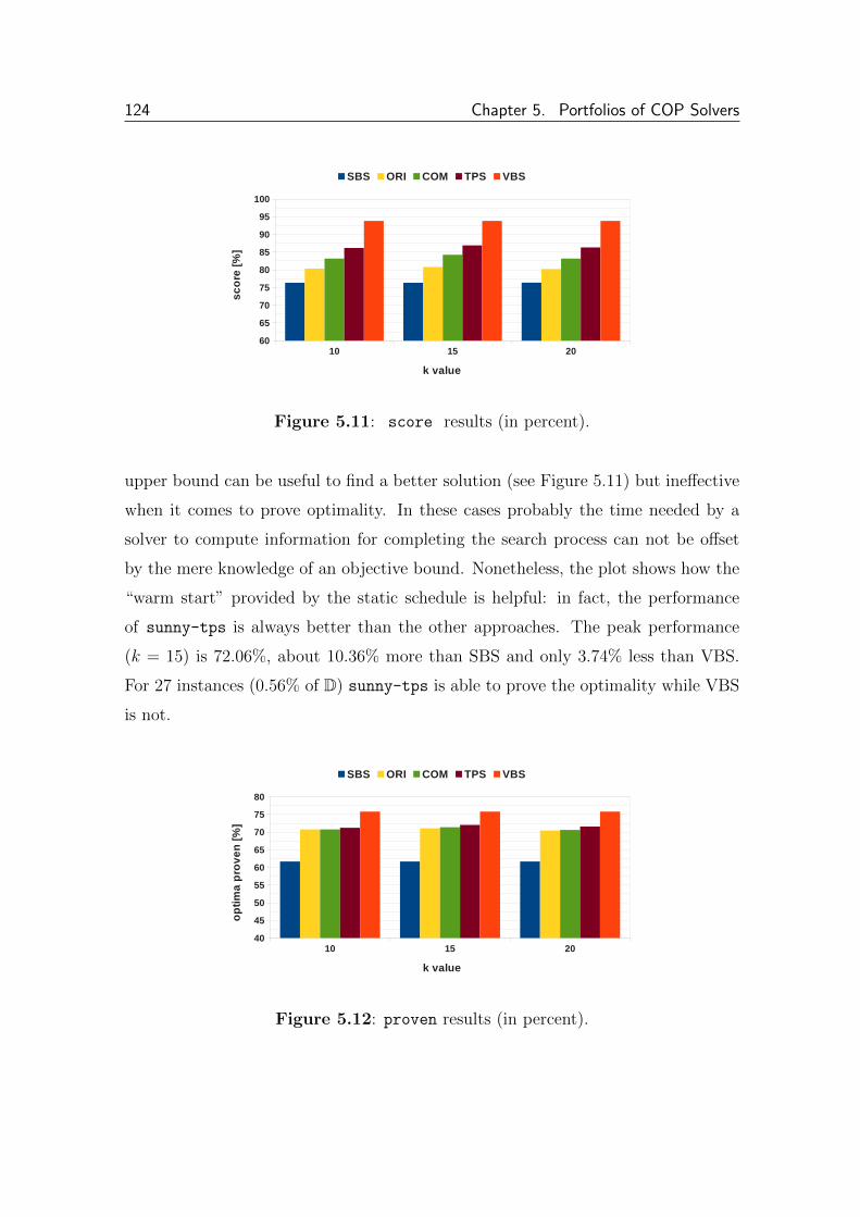
124 Chapter 5. Portfolios of COP Solvers
10 15 2060
65
70
75
80
85
90
95
100
SBS ORI COM TPS VBS
k value
sc
ore
[%
]
Figure 5.11: score results (in percent).
upper bound can be useful to find a better solution (see Figure 5.11) but ineffective
when it comes to prove optimality. In these cases probably the time needed by a
solver to compute information for completing the search process can not be offset
by the mere knowledge of an objective bound. Nonetheless, the plot shows how the
“warm start” provided by the static schedule is helpful: in fact, the performance
of sunny-tps is always better than the other approaches. The peak performance
(k = 15) is 72.06%, about 10.36% more than SBS and only 3.74% less than VBS.
For 27 instances (0.56% of D) sunny-tps is able to prove the optimality while VBS
is not.
10 15 2040
45
50
55
60
65
70
75
80
SBS ORI COM TPS VBS
k value
op
tim
a p
rov
en
[%
]
Figure 5.12: proven results (in percent).

Chapter 5. Portfolios of COP Solvers 125
Let us now focus on optimization time. In Figure 5.13 we see, in contrast to all
the score and proven results that appear to be pretty robust by varying k, a slight
discrepancy between k = 10 and k > 10. This delay time in proving optimality
is due to the scheduling order of the constituent solvers. However, for k = 15 the
results improve and for k = 20 are substantially the same. The peak performance is
achieved with k = 15 (272.61 seconds), 105.07 less than SBS and 145.9 more than
VBS; in 53 cases (1.09% of D) sunny-tps is able to prove the optimality in less time
than VBS.
10 15 200
100
200
300
400
500
600
700
800
SBS ORI COM TPS VBS
k value
op
tim
iza
tio
n t
ime
[s
ec
.]
Figure 5.13: time results (in seconds).
The area results depicted in Figure 5.14 clearly show the benefits of bounds
communication. First, note that sunny-ori is always worse than SBS: this is
because each solver scheduled by sunny-ori is executed independently, and therefore
for every solver the search is always (re-)started from scratch without exploiting
previously found solutions. sunny-com significantly improves sunny-ori, even if
its average area is very close to SBS (even worse for k = 10). The fixed schedule
run by sunny-tps often allows one to quickly find partial solutions, and thus to
noticeably outperform both sunny-ori and sunny-com. Like the time metric, the
average area is not so close to VBS (the peak performance, with k = 15, is 272.61
seconds: 132.77 seconds more than VBS, and 114.9 less than SBS), but sunny-tps
outperforms VBS in 110 cases (2.26% of D).

126 Chapter 5. Portfolios of COP Solvers
10 15 200
100
200
300
400
500
600
SBS ORI COM TPS VBS
k value
are
a [
se
c.]
Figure 5.14: area results (in seconds).
5.2.4.2 Summary
In this section we addressed the problem of boosting optimization by exploiting the
sequential cooperation of different COP solvers. A related work is [37], in which
algorithm control techniques are used to share bounds information between the
scheduled solvers without, however, explicitly rely on the solvers behaviours (as in
the technical definition we gave in Def. 5.4). In [133] the authors provide a generic
approach to knowledge sharing, which is suitable for SAT solvers but is less likely
to be useful when solvers are very disparate in nature.
Exploiting the fact that finding good solutions early can significantly improve
optimization solvers, we first provided a proper TimeSplit algorithm that relies
on the behaviour of different solvers on an instance for determining a good time-
split solver for this instance (i.e., ideally able to outperform the best solver of a
portfolio). The results show that on average the actual timesplit solver does per-
form similarly to (and sometimes even better than) the Virtual Best Solver of the
portfolio. We therefore exploited the results of TimeSplit in order to define the
Timesplit Portfolio Solver (TPS), a generic and hybrid framework that combines a
static schedule (computed off-line and run for a limited time) as well as a dynamic
schedule (computed on-line by means of a proper prediction algorithm and run in
the remaining time) for solving a new unseen instance by exploiting the bounds

Chapter 5. Portfolios of COP Solvers 127
communication between the scheduled solvers. In particular, on the one hand, we
determined the static schedule by solving a Set Covering problem according to the
results of TimeSplit on a set of training instances, and, on the other, we defined
the dynamic selection by exploiting the SUNNY algorithm. Empirical results have
shown that this idea can be beneficial and sometimes even able to outperform the
Virtual Best Solver according to different metrics that we used (i.e., score, proven,
time, and especially the new metric area) in order to evaluate the performance of
different (portfolio) solvers.
We see this work a cornerstone for portfolio approaches to solving Constraint Op-
timization Problems. Future investigations in this regard may cover the construction
of meta-portfolios, i.e., portfolio solvers consisting of other portfolio solvers. In a
way, we can see a timesplit solver TPS(p) = [(S, C), (D(p), T − C)] as a kind of
meta-portfolio: it first runs the portfolio solver (S, C), and then the portfolio solver
(D(p), T − C).
In the next chapter we show an effective tool exploiting (not only) these tech-
niques for solving hard combinatorial problems.

128 Chapter 5. Portfolios of COP Solvers

Chapter 6
sunny-cp: a CP Portfolio Solver
“Manus Multae, Cor Unum”1
As previously stressed portfolio solvers are rarely used in practice, especially
outside the walls of solving competitions. In Chapters 4 and 5 we showed several
evaluations of different portfolio approaches for solving CSPs and COPs. In par-
ticular, we proposed a number of tools —built on top of SUNNY algorithm— for
solving both CSPs (see sunny-csp in Section 4.2.3.3) and COPs (see sunny-ori,
sunny-com, and sunny-tps in Section 5.2.4). Now, we merge these two lines of re-
search by proposing sunny-cp: a new tool aimed at solving a generic CP problem,
regardless of whether it is a CSP or a COP.
The aim of sunny-cp is to provide a flexible, configurable, and usable CP port-
folio solver that can be set up and executed just like a regular individual CP solver.
To the best of our knowledge, sunny-cp is currently the only sequential portfolio
solver able to solve generic CP problems. Indeed, it was the only portfolio entrant
in the MZC 2014 [139]. In this chapter we show the architecture of sunny-cp as well
as an evaluation of its performance in the MZC 2014. As it is shown later, despite
the MZC is not (yet) the ideal scenario for a portfolio solver, sunny-cp has proved
to be competitive even in this setting.
This chapter reports an extended version of an our paper accepted in [11].
1 “Many hands, one heart”.

130 Chapter 6. sunny-cp: a CP Portfolio Solver
6.1 Architecture
In this section we illustrate the architecture of sunny-cp. We initially set up
the portfolio of sunny-cp with the solvers introduced in Section 5.2.2.3, namely:
Chuffed, CPX, G12/CBC, G12/FD, G12/Gurobi, G12/LazyFD, Gecode, and Min-
isatID. Clearly, it would have been possible to add a number of other solvers. How-
ever, from the experimental investigations reported in previous chapters it turned
out that using too large portfolios may be ineffective or sometimes even harmful. We
therefore decided to use just the eight solvers mentioned above, while still providing
the opportunity to arbitrarily change the portfolio composition.
Figure 6.1 summarizes the step-by-step execution flow of the framework from
the input CP problem to the final output outcome. The input of sunny-cp consists
of the problem instance p to be solved, the size k of the neighbourhood used by the
underlying k-NN algorithm, the solving timeout T , and the solver B of the portfolio
to be used as backup solver. Despite the portfolio described above is fixed, it is
still possible for the end user to select only a subset of its solvers. In addition, as
described below, the user can also specify the knowledge base to use for the solver(s)
selection.
The first step —that does not discriminate between CSPs and COPs— concerns
the features extraction. Given a CP problem p in input, this process identifies the
feature vector of p. By using the mzn2feat-1.0 extractor mentioned in Section 5.2.4
we extract a vector FV = 〈f1, f2, . . . , fd〉 of d = 95 features.
At step 2, the execution flow branches: if p is a CSP instance, sunny-cp uses a
knowledge base KBCSP ; otherwise, the knowledge base KBCOP is selected. Basically,
a knowledge base can be seen as a map that associates to each CP problem a
body of information relevant for the resolution process. Every CP problem of the
knowledge base belongs to a training set of already known instances, and for each
CP problem the relevant information are essentially two: its feature vector and the
solving behaviour of each constituent solver on it. sunny-cp already comes with
default knowledge bases, constructed by collecting two different datasets DCSP and

Chapter 6. sunny-cp: a CP Portfolio Solver 131
CP Problemp
1. Features Extraction
2. Features Preprocessing
3. Neighbours Identification
4. Schedule Computation
5. Problem Resolution
Outcome
BackupSolver B
PortfolioTimeout
TNeighb.Size k
KnowledgeBaseKBCOP
mzn2feat 1.0
StaticSchedule
FV
KnowledgeBaseKBCSP
INPUT PARAMETERS
CSP MODULE COP MODULE
OUTPUT
SAT. OPT. UNB.UNS. UNK.
FV'
NN
SC
Figure 6.1: sunny-cp architecture.
DCOP of CSP and COP instances retrieved from the CP instances of the MiniZinc 1.6
benchmarks, the MZCs 2012/13, and the International CSP Solver Competitions.
More in detail, DCSP (resp. DCOP ) contains 5524 (resp. 4864) instances, to each
of which is associated a feature vector of 78 (resp. 88) normalized features and the
performances of each solver of the portfolio on it. The feature vectors of KBCSP and
KBCOP differ in size since from the original 95 features extracted by mzn2feat-1.0
we removed all the constant features: as a consequence, the 10 features concerning
the objective function has been removed from the CSPs feature vectors. Moreover,
since the performances of the k-NN algorithm can be drastically degraded by the
presence of noisy or irrelevant features [6], all the features values of KBCSP and
KBCOP are scaled in the range [−1, 1]. However, note that sunny-cp also allows to
build and use other knowledge bases given as input parameters.
The original feature vector FV of the instance p is then normalized in step 2
by exploiting the information of the corresponding knowledge base. The resulting

132 Chapter 6. sunny-cp: a CP Portfolio Solver
normalized vector FV ′ = 〈f ′1, f ′2, . . . , f ′d′〉 is therefore a feature vector in which every
f ′i ∈ [−1, 1] and d′ < d (in particular, as said above, d′ = 78 if p is a CSP while
d′ = 88 if p is a COP).
The feature vector FV ′ is then used in step 3 to identify the neighbourhood NN
of p, i.e, the k instances p1, p2, . . . , pk of the selected knowledge base for which the
corresponding feature vectors FV ′1,FV ′2, . . . ,FV ′k minimize the Euclidean distance
from FV ′. The neighbourhood size k is an input parameter which is set to k = 70
unless otherwise specified. We chose this default value since it is close to the square
root of the default knowledge bases size. Indeed, the choice of k is very critical: a
simple initial approach consists in setting k =√n where n is the number of training
samples [6].
In step 4, the neighbourhood NN is used by SUNNY algorithm for computing
the schedule of solvers SC = [(s1, t1), (s2, t2), . . . , (sn, tn)] to be executed for solving
p. The selected solvers will be executed sequentially in step 5, according to the
given time limit. The default timeout T is 1800 seconds (i.e., the one used in the
last International CSP Competition) while the default backup solver B is Chuffed.
However, both T and B are options that can be specified by the end user. If a solver
aborts its execution prematurely (e.g., due to memory overflows or unsupported
constraints) its remaining execution time is allocated to the next scheduled solver,
if any, or to a not scheduled solver of the portfolio otherwise.
Note that in case p is a CSP the scheduled solvers are executed independently,
i.e., there is no cooperation and communication between them.2 If instead p is a
COP instance, sunny-cp runs a timesplit solver (see Def. 5.5): it exploits the best
solution found by a solver for narrowing the search space of the following ones as seen
in Section 5.2. If p is a CSP, sunny-cp may output three alternatives: satisfiable
(a solution exists for p), unsatisfiable (p has no solutions) or unknown (sunny-cp is
not able to say anything about p). If p is a COP, there are two more alternatives:
2sunny-cp views the constituent CSP solvers as “black boxes”. The lack of a standard protocol
to extract and share knowledge between solvers makes it hard to communicate potentially useful
information like nogoods.
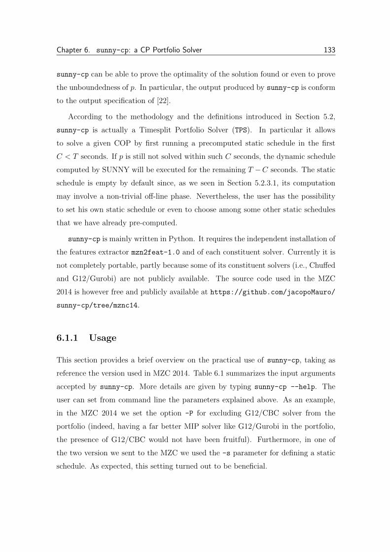
Chapter 6. sunny-cp: a CP Portfolio Solver 133
sunny-cp can be able to prove the optimality of the solution found or even to prove
the unboundedness of p. In particular, the output produced by sunny-cp is conform
to the output specification of [22].
According to the methodology and the definitions introduced in Section 5.2,
sunny-cp is actually a Timesplit Portfolio Solver (TPS). In particular it allows
to solve a given COP by first running a precomputed static schedule in the first
C < T seconds. If p is still not solved within such C seconds, the dynamic schedule
computed by SUNNY will be executed for the remaining T −C seconds. The static
schedule is empty by default since, as we seen in Section 5.2.3.1, its computation
may involve a non-trivial off-line phase. Nevertheless, the user has the possibility
to set his own static schedule or even to choose among some other static schedules
that we have already pre-computed.
sunny-cp is mainly written in Python. It requires the independent installation of
the features extractor mzn2feat-1.0 and of each constituent solver. Currently it is
not completely portable, partly because some of its constituent solvers (i.e., Chuffed
and G12/Gurobi) are not publicly available. The source code used in the MZC
2014 is however free and publicly available at https://github.com/jacopoMauro/
sunny-cp/tree/mznc14.
6.1.1 Usage
This section provides a brief overview on the practical use of sunny-cp, taking as
reference the version used in MZC 2014. Table 6.1 summarizes the input arguments
accepted by sunny-cp. More details are given by typing sunny-cp --help. The
user can set from command line the parameters explained above. As an example,
in the MZC 2014 we set the option -P for excluding G12/CBC solver from the
portfolio (indeed, having a far better MIP solver like G12/Gurobi in the portfolio,
the presence of G12/CBC would not have been fruitful). Furthermore, in one of
the two version we sent to the MZC we used the -s parameter for defining a static
schedule. As expected, this setting turned out to be beneficial.
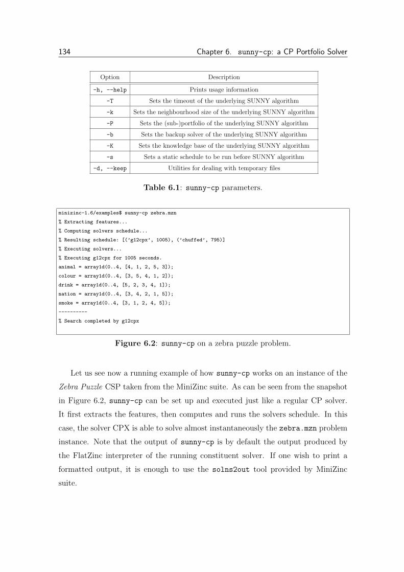
134 Chapter 6. sunny-cp: a CP Portfolio Solver
Option Description
-h, --help Prints usage information
-T Sets the timeout of the underlying SUNNY algorithm
-k Sets the neighbourhood size of the underlying SUNNY algorithm
-P Sets the (sub-)portfolio of the underlying SUNNY algorithm
-b Sets the backup solver of the underlying SUNNY algorithm
-K Sets the knowledge base of the underlying SUNNY algorithm
-s Sets a static schedule to be run before SUNNY algorithm
-d, --keep Utilities for dealing with temporary files
Table 6.1: sunny-cp parameters.
minizinc-1.6/examples$ sunny-cp zebra.mzn
% Extracting features...
% Computing solvers schedule...
% Resulting schedule: [(’g12cpx’, 1005), (’chuffed’, 795)]
% Executing solvers...
% Executing g12cpx for 1005 seconds.
animal = array1d(0..4, [4, 1, 2, 5, 3]);
colour = array1d(0..4, [3, 5, 4, 1, 2]);
drink = array1d(0..4, [5, 2, 3, 4, 1]);
nation = array1d(0..4, [3, 4, 2, 1, 5]);
smoke = array1d(0..4, [3, 1, 2, 4, 5]);
----------
% Search completed by g12cpx
Figure 6.2: sunny-cp on a zebra puzzle problem.
Let us see now a running example of how sunny-cp works on an instance of the
Zebra Puzzle CSP taken from the MiniZinc suite. As can be seen from the snapshot
in Figure 6.2, sunny-cp can be set up and executed just like a regular CP solver.
It first extracts the features, then computes and runs the solvers schedule. In this
case, the solver CPX is able to solve almost instantaneously the zebra.mzn problem
instance. Note that the output of sunny-cp is by default the output produced by
the FlatZinc interpreter of the running constituent solver. If one wish to print a
formatted output, it is enough to use the solns2out tool provided by MiniZinc
suite.

Chapter 6. sunny-cp: a CP Portfolio Solver 135
minizinc-1.6/benchmarks/rcpsp$ sunny-cp -s g12cpx,1,minisatid,250 rcpsp.mzn J120_9_6.dzn
% Extracting features...
% Computing solvers schedule...
% Resulting schedule: [(’g12cpx’, 1), (’minisatid’, 250), (’gecode’, 740.6350744504846),
(’minisatid’, 451.8984479634444), (’chuffed’, 356.466477586071)]
% Executing solvers...
% Executing g12cpx for 1 seconds.
% o__b__j__v__a__r = 117;
objective = 117;
----------
% ...Omitting other sub-optimal solutions (objective = 115, 112, ..., 102) found by CPX ...
----------
% o__b__j__v__a__r = 101;
objective = 101;
----------
% o__b__j__v__a__r = 101
% Search not yet completed.
% Adding constraint objective < 101
% Executing minisatid for 250 seconds.
objective = 100;
% o__b__j__v__a__r = 100;
----------
objective = 99;
% o__b__j__v__a__r = 99;
----------
objective = 98;
% o__b__j__v__a__r = 98;
----------
% Search completed by minisatid
==========
Figure 6.3: sunny-cp on a RCPSP problem. For the sake of readability, the sub-
optimal solutions 115, 112, ..., 102 found by CPX, as well as other output variables,
are here omitted.
We conclude the section by showing how sunny-cp behaves on the example
depicted in Figure 5.10, where an instance of the RCPSP minimization problem is
solved by the timesplit solver [(CPX, 1), (MinisatID, 1799)]. For running such sched-
ule solver we simply impose a corresponding static schedule via the -s option, as
shown in Figure 6.3. Note that in this case we set a timeout of 250 seconds for
MinisatID: if after that time the instance is still not solved the dynamic schedule

136 Chapter 6. sunny-cp: a CP Portfolio Solver
returned by SUNNY is run in the remaining 1800− (1 + 250) = 1549 seconds. How-
ever, as already shown in the example of Figure 5.10, MinisatID is able to complete
the search in less than 250 seconds by exploiting the bound 101 instantaneously
found by CPX. Note also that for solving COPs sunny-cp introduces an auxiliary
variable called o b j v a r for keeping track of the best value found so far (and,
consequently, for possibly injecting that bound to the next scheduled solvers).
6.2 Validation
Extensive evaluations of SUNNY against different state-of-the-art approaches have
been reported in Chapters 4 and 5 by using big test sets (i.e., about 500 instances
or more) and fairly large solving timeouts (i.e., T = 1800 seconds). All these
empirical evaluations has proven the effectiveness of SUNNY, in particular w.r.t. the
constituent solvers of its portfolio that have been always greatly outperformed. In
this section we show instead how sunny-cp behaved in the MZC 2014. In this
setting things are different: the test set is far smaller (i.e., 100 instances, almost
always satisfiable), the timeout is lower (900 seconds), and especially a different
evaluation metric is adopted w.r.t. the proven, time, score, and area metrics
introduced in Def. 4.1, 4.2, 5.1, 5.2, 5.3, 5.6. Indeed, the MiniZinc Challenge Score
(MZCS) introduced in Section 5.1.1 and evaluated —by means of simulations— in
Section 5.1.3.4 is based on a Borda count voting system [42] where each CP problem
is treated like a voter who ranks the solvers, and each solver gets a score proportional
to the number of solvers it beats.
Two versions of sunny-cp attended the competition: sunny-cp-open and sunny-
cp-presolve-open. The first is the default sunny-cp solver as described in Section
6.1. The second is instead the variant that runs for every COP a static schedule
in the first 30 seconds. In particular the solvers Chuffed, Gecode, and CPX are
executed for 10 seconds each. Note that, in contrast to what done in 5.2.3.1, no Set
Covering problem was solved for computing the static schedule. The static schedule
used in the competition was set ”by hand“ after some empirical investigations, with

Chapter 6. sunny-cp: a CP Portfolio Solver 137
the main goal of quickly solving the easiest instances. ”-open“ refers to open search
category, i.e., the track in which sunny-cp competed.
The results of such track are summarized in Table 6.2. Before discussing the
results, it is appropriate to make a few remarks.
SOLVER SCORE
Chuffed-free* 1324.02
OR-Tools-par (GOLD MEDAL) 1084.97
Opturion CPX-free (SILVER MEDAL) 1079.02
sunny-cp-presolve-open 1064.46
Choco-par (BRONZE MEDAL) 1005.61
iZplus-par 994.32
sunny-cp-open 967.14
G12/LazyFD-free* 782.78
HaifaCSP-free 779.72
Gecode-par 720.97
SICStus Prolog-fd 708.51
Mistral-free 703.56
MinisatID-free* 587.24
Picat SAT-free 586.64
JaCoP-fd 549.24
G12/FD-free* 526.26
Picat CP-free 402.88
Concrete-free 353.24
Table 6.2: MZC 2014 open track. Parallel solvers are in italics, while the solvers
included in sunny-cp are marked with *.
First, the open class includes also parallel solvers. This can be disadvantageous
for sequential solvers like sunny-cp that do not exploit more computation units.
Second, in the MZC the solving time time(p, s) refers to the time needed by s for
solving the FlatZinc model ps resulting from the conversion of the original MiniZinc
138 Chapter 6. sunny-cp: a CP Portfolio Solver
model p to ps, thus ignoring the solver dependent time needed to flatten p in ps.
The choice of discarding the conversion penalizes a portfolio solver. Indeed, given
the heterogeneous nature of our portfolio, sunny-cp can not use global redefinitions
that are suitable for all its constituent solvers. Therefore, differently from all the
other solvers of the open search track, the result of sunny-cp were computed by
considering not only the solving time of the FlatZinc models but also all the conver-
sion times of the MiniZinc input, including an initial conversion to FlatZinc required
for extracting the feature vector of p. Moreover, as we seen in Section 5.1.1, the
grading methodology of MZC further penalizes a portfolio solver because in case
of ties it may assign a score that is disproportionate w.r.t. the solving time differ-
ence. This is a drawback for sunny-cp since, even if it selects the best constituent
solver, it requires an additional amount of time for extracting the features and for
the solver selection. This holds especially in the presence of a clear dominant solver,
like Chuffed for the MZC 2014. All these difficulties have been recognized by the
organizers, which awarded to sunny-cp an honourable mention.3
Let us now analyse the results. As said, if on the one hand having Chuffed in
the portfolio was undoubtedly advantageous for us, on the other hand this can also
be counterproductive. Indeed, it is impossible to beat it in the numerous times in
which it is the best solver, even if sunny-cp selects it to solve the instance. Moreover,
note that the other solvers of sunny-cp enrolled in the Challenge have not achieved
excellent performance: G12/LazyFD is 8th, MinisatID is 13th and G12/FD is 16th.
Gecode-par is 10th, but sunny-cp did not use this version since Gecode-par is a
parallel solver. Finally, G12/CBC, G12/Gurobi, and CPX have not attended the
challenge.4 This setting is inevitably detrimental for a portfolio. There is a clearly
dominant constituent solver, while the others have a rather low contribution. To
boost the performances of sunny-cp we could have used an ’ad hoc’ training set for
the MZC. Indeed, as pointed out also in [176], the good results of a portfolio solver
3sunny-cp was not eligible for prizes, since it contains solvers developed by the MZC organizers.4 Note that Gecode-free, the sequential version of Gecode-par, in the open category would
be ranked 12th. Opturion CPX[150] is instead based on CPX, but it is not CPX. Moreover the
constituent solvers of the portfolio may be obsolete w.r.t. the version submitted to MZC 2014.
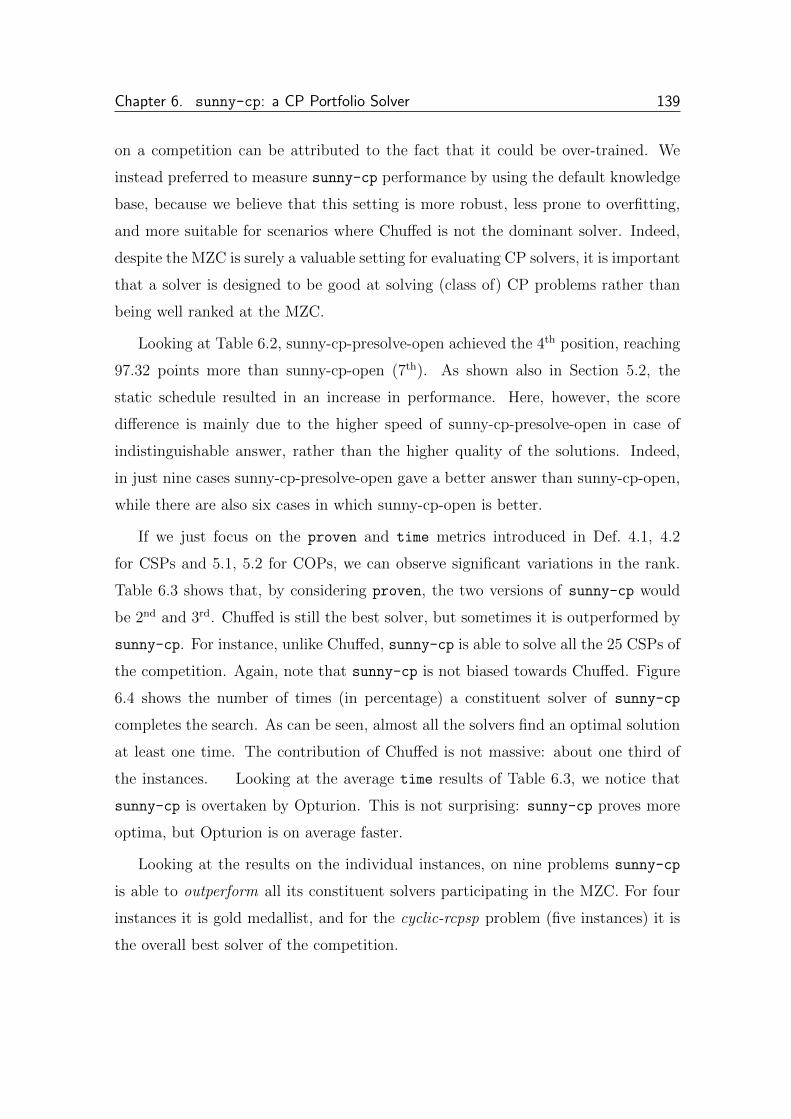
Chapter 6. sunny-cp: a CP Portfolio Solver 139
on a competition can be attributed to the fact that it could be over-trained. We
instead preferred to measure sunny-cp performance by using the default knowledge
base, because we believe that this setting is more robust, less prone to overfitting,
and more suitable for scenarios where Chuffed is not the dominant solver. Indeed,
despite the MZC is surely a valuable setting for evaluating CP solvers, it is important
that a solver is designed to be good at solving (class of) CP problems rather than
being well ranked at the MZC.
Looking at Table 6.2, sunny-cp-presolve-open achieved the 4th position, reaching
97.32 points more than sunny-cp-open (7th). As shown also in Section 5.2, the
static schedule resulted in an increase in performance. Here, however, the score
difference is mainly due to the higher speed of sunny-cp-presolve-open in case of
indistinguishable answer, rather than the higher quality of the solutions. Indeed,
in just nine cases sunny-cp-presolve-open gave a better answer than sunny-cp-open,
while there are also six cases in which sunny-cp-open is better.
If we just focus on the proven and time metrics introduced in Def. 4.1, 4.2
for CSPs and 5.1, 5.2 for COPs, we can observe significant variations in the rank.
Table 6.3 shows that, by considering proven, the two versions of sunny-cp would
be 2nd and 3rd. Chuffed is still the best solver, but sometimes it is outperformed by
sunny-cp. For instance, unlike Chuffed, sunny-cp is able to solve all the 25 CSPs of
the competition. Again, note that sunny-cp is not biased towards Chuffed. Figure
6.4 shows the number of times (in percentage) a constituent solver of sunny-cp
completes the search. As can be seen, almost all the solvers find an optimal solution
at least one time. The contribution of Chuffed is not massive: about one third of
the instances. Looking at the average time results of Table 6.3, we notice that
sunny-cp is overtaken by Opturion. This is not surprising: sunny-cp proves more
optima, but Opturion is on average faster.
Looking at the results on the individual instances, on nine problems sunny-cp
is able to outperform all its constituent solvers participating in the MZC. For four
instances it is gold medallist, and for the cyclic-rcpsp problem (five instances) it is
the overall best solver of the competition.
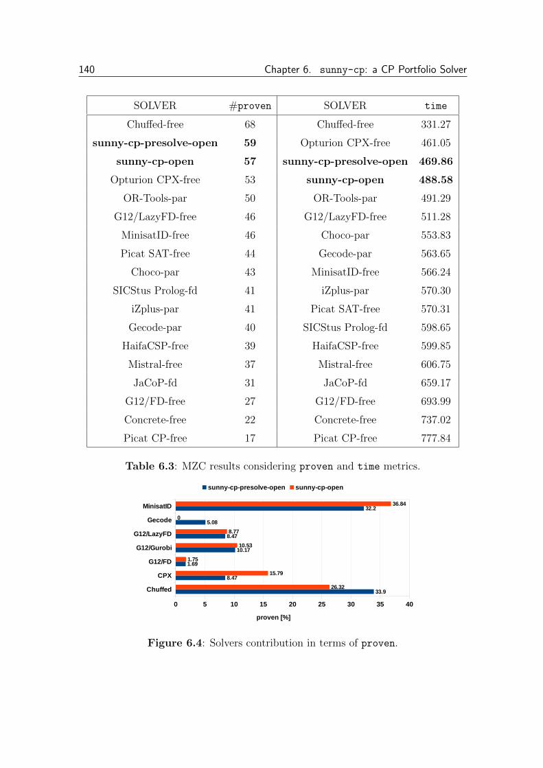
140 Chapter 6. sunny-cp: a CP Portfolio Solver
SOLVER #proven SOLVER time
Chuffed-free 68 Chuffed-free 331.27
sunny-cp-presolve-open 59 Opturion CPX-free 461.05
sunny-cp-open 57 sunny-cp-presolve-open 469.86
Opturion CPX-free 53 sunny-cp-open 488.58
OR-Tools-par 50 OR-Tools-par 491.29
G12/LazyFD-free 46 G12/LazyFD-free 511.28
MinisatID-free 46 Choco-par 553.83
Picat SAT-free 44 Gecode-par 563.65
Choco-par 43 MinisatID-free 566.24
SICStus Prolog-fd 41 iZplus-par 570.30
iZplus-par 41 Picat SAT-free 570.31
Gecode-par 40 SICStus Prolog-fd 598.65
HaifaCSP-free 39 HaifaCSP-free 599.85
Mistral-free 37 Mistral-free 606.75
JaCoP-fd 31 JaCoP-fd 659.17
G12/FD-free 27 G12/FD-free 693.99
Concrete-free 22 Concrete-free 737.02
Picat CP-free 17 Picat CP-free 777.84
Table 6.3: MZC results considering proven and time metrics.
Chuffed
CPX
G12/FD
G12/Gurobi
G12/LazyFD
Gecode
MinisatID
0 5 10 15 20 25 30 35 40
33.9
8.47
1.69
10.17
8.47
5.08
32.2
26.32
15.79
1.75
10.53
8.77
0
36.84
sunny-cp-presolve-open sunny-cp-open
proven [%]
Figure 6.4: Solvers contribution in terms of proven.

Chapter 6. sunny-cp: a CP Portfolio Solver 141
We conclude the section by proposing an alternative ranking system. As pre-
viously mentioned, we realized that, in case of indistinguishable answer between
two solvers, in the MZC the gain of a solver depends on the runtime ratio rather
than the runtime difference. For instance, let us suppose that two solvers s0 and
s1 solve a problem p in 1 and 2 second respectively. The score assigned to s0 is
2/3 = 0.667 while s1 scores 1/3 = 0.333. The same score would be reached by the
two solvers if time(p, s1) = 2 ∗ time(p, s0). Hence, if for example time(p, s0) = 400
and time(p, s1) = 800, the difference between the scores of s0 and s1 would be the
same even if the absolute time difference is 1 second in the first case, 400 seconds
in the second. In our opinion, this scoring methodology could overestimate small
time differences in case of easy instances, as well as underrate big time differences
in case of medium and hard instances. A possible workaround to this problem is to
assign each solver a score in [0, 1] that, in case of indistinguishable answer between
two solvers, is linearly proportional to the solving time difference. We then propose
a modified metric MZC-MOD that differs from the MZC score since, when the answers
of s0 and s1 are indistinguishable, it gives to the solvers a ”reward“ such that:
MZC-MOD(p, si) = 0.5 +time(p, s1−i)− time(p, si)
2Ti ∈ {0, 1}
where T is the timeout (i.e., 900 seconds for MZC).
With this new metric, according to the previous examples, if time(p, s0) = 1
and time(p, s1) = 2, then the score difference is minimal since MZC-MOD(p, s0) =
0.5 + 1/2 ∗ 900 = 0.501 and MZC-MOD(p, s1) = 0.5− 1/2 ∗ 900 = 0.499. In contrast, if
time(p, s0) = 400 and time(p, s1) = 800 then the difference is proportionally higher:
MZC-MOD(p, s0) = 0.722 and MZC-MOD(p, s1) = 0.278.
Figure 6.5 depicts the effects of using MZC-MOD in place of MZC score w.r.t. the
first seven positions of the ranking. The classification with the new score is much
more compact and reflects the lower impact of the solving time difference in case of
identical answers. Chuffed is firmly in the lead, but if compared to the original score
loses about 165 points. Except for sunny-cp and Choco, all other approaches have
a deterioration of performance. In particular, sunny-cp-presolve-open gains 19.82

142 Chapter 6. sunny-cp: a CP Portfolio Solver
Chuffed-free
OR-Tools-par
Opturion CPX-free
sunny-cp-presolve-open
Choco-par
iZplus-par
sunny-cp-open
900 950 1000 1050 1100 1150 1200 1250 1300
1159.12
1081.73
992.29
1084.28
1025.05
961.21
1007.12
MZC MZC-MOD
Score
Figure 6.5: Score differences between MZC score and MZC-MOD.
points surpassing OR-Tools-par in the 2nd position. Even more noticeable is the
score improvement of sunny-cp-open, that earns about 40 points and 2 positions in
the ranking.
6.3 Summary
In this chapter we described sunny-cp, a sequential portfolio solver able to solve both
satisfaction and optimization problems defined in MiniZinc language. sunny-cp is
aimed to provide a flexible, configurable, and usable CP portfolio solver that can be
set up and executed by the end users just like an usual, single CP solver.
Since we already verified in former evaluations the effectiveness of sunny-cp
when validated on heterogeneous and large sets of test instances, in this section we
focused on the results obtained by two versions of sunny-cp in the MiniZinc Chal-
lenge 2014. Despite the grading mechanism of the challenge may penalize a sequen-
tial portfolio solver, sunny-cp turned out to be competitive even when compared
to parallel solvers, and it was sometimes even able to outperform state-of-the-art
constraint solvers. In this regard, we also proposed and evaluated an alternative
scoring system that, in case of indistinguishable quality of the solutions, takes into
account the solving time difference in a more linear way.
Our claim about sunny-cp is not related to the introduction of a new approach,
but concerns the presentation of a new tool that could serve as a baseline for future

Chapter 6. sunny-cp: a CP Portfolio Solver 143
developments. We hope that sunny-cp can take a step forward in encouraging and
disseminating the actual use of CP portfolio solvers.
There is plenty of lines of research that can be explored in order to extend the ca-
pabilities of sunny-cp. For examples, the selection strategies of [114, 151, 132], the
impact of using different distance metrics and features [124], the robustness towards
the neighbourhood size of k-NN algorithm [10], the automated tuning of different
solvers configurations [114], the use of benchmark generation techniques [102], the
evaluation of different ranking methods [26, 75]. Certainly one of the most promising
directions for further research is the extension of sunny-cp to a parallel environ-
ment, where multiple cores can be used to launch more than one constituent solver
in parallel. In this setting it may be important to devise and evaluate coopera-
tive strategies between the constituent solvers, by exploiting and sharing tokens of
knowledge like the nogoods generated by the lazy clause generation solvers.

144 Chapter 6. sunny-cp: a CP Portfolio Solver

Chapter 7
Conclusions and Extensions
“Ite, missa est”1
“Multae Manus Onus Levant” is a Latin motto that literally means “Many hands
lighten the load”. If we see the hands like different constraint solvers, and the
load like an hard combinatorial problem to be solved, we can get an idea of the
underlying logic of portfolio solvers. In this thesis we investigated the benefits of
portfolio solving in the CP context, trying to improve a state-of-the-art that in such
a setting still turns out to be rather immature and unexplored. We have embarked
on a path of investigations, observations, insights, implementations, and extensive
evaluations. We decided to first start with CSPs, which are closer to SAT problems
(that can be in turn be seen as particular cases of CSPs). Then, we moved to the
less explored field of portfolio approaches for solving COPs. Being a COP more
general than a CSP, here things become more complicated and, at the same time,
more challenging. The promising results observed in these experimental evaluations
led us to merge these two lines of research for building sunny-cp, a prototype for
a new generation CP portfolio solver. More in detail, the original contributions of
this thesis are the following:
1 Concluding Latin words addressed to the people in the Mass of the Roman Rite, as well as
the Lutheran Divine Service.

146 Chapter 7. Conclusions and Extensions
• we performed several empirical evaluations of different portfolio approaches
for solving both CSPs and COPs. We think that these comparative studies,
that required a considerable effort, can be an useful baseline to compare and
develop new portfolio approaches;
• we provided the full support of MiniZinc, nowadays a de-facto standard for
modelling and solving CP problems, while still retaining the compatibility
with XCSP format. In particular, we developed tools for converting a XCSP
instance to MiniZinc (i.e., xcsp2mzn) and for retrieving an extensive set of
features from a MiniZinc model (i.e., mzn2feat);
• we developed SUNNY, a lazy portfolio approach for constraint solving. SUN-
NY is a simple and flexible algorithm portfolio that, without building an ex-
plicit prediction model, predicts a schedule of the constituent solvers for solving
a given problem. The good performances reached by SUNNY on CSPs led us
to extend it to COPs and to build some prototypes of CSP/COP portfolio
solvers (i.e., sunny-csp, sunny-ori, sunny-com, and sunny-tps);
• we took a step forward towards the definition of COP portfolios. We intro-
duced new metrics like score and area and we studied how CSP portfolio
solvers might be adapted to deal with COPs. In particular, since COP solvers
may yield sub-optimal solutions before finding the best one, we addressed the
problem of boosting optimization by exploiting the sequential cooperation of
different COP solvers. Empirical results showed that this approach may even
allow to outperform the best solver of the portfolio;
• we finally reaped the benefits of our work for developing sunny-cp: a new
tool aimed at solving a generic CP problem, regardless of whether it is a CSP
or a COP. The aim of sunny-cp is to provide a flexible, configurable, and
usable CP portfolio solver that can be set up and executed just like a regular
individual CP solver. To the best of our knowledge, sunny-cp is currently the
only sequential portfolio solver able to solve generic CP problems.
Chapter 7. Conclusions and Extensions 147
We think that this work could serve as a cornerstone for the effective use and
dissemination of portfolios in (and also outside) the CP field. Indeed, despite the
proven effectiveness showed in several experiments, the actual use of portfolio solvers
is pretty limited and usually confined to annual competitions. This is obviously
restrictive: if for winning a competition based on relatively few instances a portfolio
solver requires a year of training, it is evident that its usability in other settings
is practically zero. There is plenty of future directions. For instance, you might
consider well-known problems like feature selection, dataset filtering, or algorithm
configuration. Other interesting investigations could be the impact assessment of
different performance metrics, or the inclusion in the portfolio of incomplete, non-
deterministic solvers like local search solvers.
We identified in particular four main challenges for the future of CP portfolio
solvers:
• prediction model : often the prediction model responsible for the solver selec-
tion requires an heavy training phase. We think that one of the main future
directions for portfolio solvers is the reduction of the training costs. For in-
stance, the SUNNY approach can not be defined purely dynamic: it still needs
a detailed knowledge base for making predictions. Making the portfolio solvers
more flexible and dynamic could certainly be useful in the future.
• optimization problem: since the state of the art for COP portfolios is still
in an embryonic stage, we think that a deepening on optimization problems
is needed. We suggest to insist on collaborative portfolios able to exchange
information between the constituent solvers. Given the benefits of bounds
communication, it would be interesting to share also other information (e.g.,
redundant constraints like nogoods).
• parallelisation: working with different solvers in parallel is less trivial than
thought at first, and it is not only a matter of software engineering. Syn-
chronization and memory consumption issues arise, and the communication
between constituent solvers is not so straight as for sequential portfolios. This

148 Chapter 7. Conclusions and Extensions
direction could open interesting streams of research, especially when applied
to optimization problems.
• utilization: facilitating the practical use of portfolio solvers for solving generic
CP problems is desirable. As an example, we realized that is often very difficult
to use the original portfolio solver for making experiments. It would certainly
be a good practice in the future to the develop free and usable code and APIs
for encouraging the spread of CP portfolio solvers, as well as having standard
benchmarks and a standard language for encoding CP problems.
We are currently addressing these challenges by developing a more configurable
and usable version of sunny-cp, also capable of exploiting the simultaneous and
cooperative execution of its constituent solvers in a multicore setting.
References
[1] Choco Solver. http://www.emn.fr/z-info/choco-Solver/.
[2] iZplus Solver (description). http://www.minizinc.org/challenge2014/
description_izplus.txt.
[3] OR-Tools — The Google Operations ReSearch Suite. https://code.google.
com/p/or-tools/.
[4] Ignasi Abıo and Peter J. Stuckey. Encoding Linear Constraints into SAT. In
CP, pages 75–91, 2014.
[5] Abderrahmane Aggoun and Nicolas Beldiceanu. Extending CHIP in Order
to Solve Complex Scheduling and Placement Problems. In JFPL, pages 51–,
1992.
[6] Naomi S. Altman. An Introduction to Kernel and Nearest-Neighbor Nonpara-
metric Regression. The American Statistician, 46(3):175–185, 1992.
[7] Roberto Amadini, Maurizio Gabbrielli, and Jacopo Mauro. An Empirical
Evaluation of Portfolios Approaches for Solving CSPs. In CPAIOR, volume
7874 of LNCS, pages 316–324. Springer, 2013.
[8] Roberto Amadini, Maurizio Gabbrielli, and Jacopo Mauro. An Enhanced
Features Extractor for a Portfolio of Constraint Solvers. In SAC, pages 1357–
1359. ACM, 2014.

150 References
[9] Roberto Amadini, Maurizio Gabbrielli, and Jacopo Mauro. Portfolio Ap-
proaches for Constraint Optimization Problems. In LION, volume 8426 of
LNCS, pages 21–35. Springer, 2014.
[10] Roberto Amadini, Maurizio Gabbrielli, and Jacopo Mauro. SUNNY: a Lazy
Portfolio Approach for Constraint Solving. TPLP, 14(4-5):509–524, 2014.
[11] Roberto Amadini, Maurizio Gabbrielli, and Jacopo Mauro. SUNNY-CP: a
Sequential CP Portfolio Solver. In SAC, 2015.
[12] Roberto Amadini and Peter J. Stuckey. Sequential Time Splitting and Bounds
Communication for a Portfolio of Optimization Solvers. In CP, volume 8656
of LNCS, pages 108–124. Springer, 2014.
[13] Carlos Ansotegui, Meinolf Sellmann, and Kevin Tierney. Gender-Based Ge-
netic Algorithm for the Automatic Configuration of Algorithms. In CP, volume
5732 of LNCS, pages 142–157. Springer, 2009.
[14] Alejandro Arbelaez, Youssef Hamadi, and Michele Sebag. Continuous Search
in Constraint Programming. In ICTAI, pages 53–60. IEEE Computer Society,
2010.
[15] Sylvain Arlot and Alain Celisse. A Survey of Cross-Validation Procedures for
Model Selection. Statistics Surveys, 4:40–79, 2010.
[16] Gilles Audemard, Benoıt Hoessen, Saıd Jabbour, Jean-Marie Lagniez, and
Cedric Piette. PeneLoPe, a Parallel Clause-Freezer Solver. In SAT Challenge
2012, pages 43–44, 2012.
[17] Francisco Azevedo. Cardinal: A Finite Sets Constraint Solver. Constraints,
12(1):93–129, 2007.
[18] Pedro Barahona, Steffen Holldobler, and Van-Hau Nguyen. Representative
Encodings to Translate Finite CSPs into SAT. In CPAIOR, pages 251–267,
2014.
References 151
[19] Clark W. Barrett, Roberto Sebastiani, Sanjit A. Seshia, and Cesare Tinelli.
Satisfiability Modulo Theories. In Handbook of Satisfiability, pages 825–885.
2009.
[20] Roman Bartak. History of Constraint Programming. John Wiley and Sons,
Inc., 2010.
[21] Roberto Battiti and Marco Protasi. Approximate Algorithms and Heuristics
for MAX-SAT. In Handbook of Combinatorial Optimization, pages 77–148.
Springer, 1999.
[22] Ralph Becket. Specification of FlatZinc — Version 1.6. http://www.
minizinc.org/downloads/doc-1.6/flatzinc-spec.pdf, 2014.
[23] Mohammed Said Belaid, Claude Michel, and Michel Rueher. Boosting Local
Consistency Algorithms over Floating-Point Numbers. In CP, CP’12, pages
127–140, Berlin, Heidelberg, 2012. Springer-Verlag.
[24] Nicolas Beldiceanu, Mats Carlsson, Sophie Demassey, and Thierry Petit.
Global Constraint Catalogue: Past, Present and Future. Constraints,
12(1):21–62, 2007.
[25] Anton Belov, Daniel Diepold, Marijn Heule, and Matti Jarvisalo, editors. Pro-
ceedings of SAT Competition 2014: Solver and Benchmark Descriptions, vol-
ume B-2014-2 of Department of Computer Science Series of Publications B.
University of Helsinki, 2014. ISBN 978-951-51-0043-6.
[26] Daniel Le Berre and Laurent Simon. Preface. JSAT, 2006.
[27] Timo Berthold. Measuring the impact of primal heuristics. Operations Re-
Search Letters, 41(6):611–614, 2013.
[28] Christian Bessiere, Zeynep Kiziltan, Andrea Rappini, and Toby Walsh. A
Framework for Combining Set Variable Representations. In SARA, 2013.

152 References
[29] Stefano Bistarelli, Ugo Montanari, and Francesca Rossi. Constraint Solving
over Semi-rings. In IJCAI, pages 624–630, 1995.
[30] Stefano Bistarelli, Ugo Montanari, and Francesca Rossi. Semiring-Based Con-
straint Satisfaction and Optimization. J. ACM, 44(2):201–236, March 1997.
[31] Stefano Bistarelli, Ugo Montanari, Francesca Rossi, Thomas Schiex, Gerard
Verfaillie, and Helene Fargier. Semiring-Based CSPs and Valued CSPs: Frame-
works, Properties, and Comparison. Constraints, 4(3):199–240, 1999.
[32] Bernard Botella, Arnaud Gotlieb, and Claude Michel. Symbolic Execution of
Floating-Point Computations: ReSearch Articles. Softw. Test. Verif. Reliab.,
16(2):97–121, June 2006.
[33] Stephen Boyd and Lieven Vandenberghe. Convex Optimization. Cambridge
University Press, New York, NY, USA, 2004.
[34] Peter Brucker, Andreas Drexl, Rolf Mohring, Klaus Neumann, and Erwin
Pesch. Resource-Constrained Project Scheduling: Notation, Classification,
Models, and Methods. European journal of operational reSearch, 112(1):3–41,
1999.
[35] Hans Kleine Buning, Marek Karpinski, and Andreas Flogel. Resolution for
Quantified Boolean Formulas. Information and Computation, 117(1):12–18,
1995.
[36] Tom Carchrae. Low Knowledge Algorithm Control for Constraint-Based
Scheduling. PhD thesis, Department of Computer Science, National University
of Ireland, 2009.
[37] Tom Carchrae and J. Christopher Beck. Low-Knowledge Algorithm Control.
In AAAI, pages 49–54, 2004.

References 153
[38] Tom Carchrae and J. Christopher Beck. Applying Machine Learning to Low-
Knowledge Control of Optimization Algorithms. Computational Intelligence,
21(4):372–387, 2005.
[39] Yves Caseau, Francois Laburthe, and Glenn Silverstein. A Meta-Heuristic
Factory for Vehicle Routing Problems. In CP, pages 144–158. Springer, 1999.
[40] Amedeo Cesta, Angelo Oddi, and Stephen F Smith. A Constraint-Based
Method for Project Scheduling with Time Windows. Journal of Heuristics,
8(1):109–136, 2002.
[41] Nitesh V. Chawla, Kevin W. Bowyer, Lawrence O. Hall, and W. Philip
Kegelmeyer. SMOTE: Synthetic Minority Over-sampling Technique. Jour-
nal of Artificial Intelligence ReSearch, 16, 2002.
[42] Yann Chevaleyre, Ulle Endriss, Jerome Lang, and Nicolas Maudet. A Short
Introduction to Computational Social Choice. In SOFSEM. 2007.
[43] David A. Cohen, Peter Jeavons, Christopher Jefferson, Karen E. Petrie, and
Barbara M. Smith. Symmetry Definitions for Constraint Satisfaction Prob-
lems. Constraints, 11(2-3):115–137, 2006.
[44] Andrew R. Conn, Nicholas I.M. Gould, Annick Sartenaer, and Philippe L.
Toint. Convergence Properties of an Augmented Lagrangian Algorithm for
Optimization with a Combination of General Equality and Linear Constraints.
SIAM J. on Optimization, 6(3):674–703, March 1996.
[45] Stephen A. Cook. The Complexity of Theorem-Proving Procedures. In STOC,
pages 151–158. ACM, 1971.
[46] Opturion — CPX Discrete Optimiser. http://www.opturion.com/cpx.html.
[47] James Crawford, Matthew Ginsberg, Eugene Luks, and Amitabha Roy.
Symmetry-Breaking Predicates for Search Problems. pages 148–159. Morgan
Kaufmann, 1996.

154 References
[48] George B. Dantzig and John H. Ramser. The Truck Dispatching Problem.
Management science, 6(1):80–91, 1959.
[49] Bruno De Backer, Vincent Furnon, Paul Shaw, Philip Kilby, and Patrick
Prosser. Solving Vehicle Routing Problems using Constraint Programming
and MetaHeuristics. Journal of Heuristics, 6(4):501–523, 2000.
[50] Broes de Cat, Bart Bogaerts, Jo Devriendt, and Marc Denecker. Model Ex-
pansion in the Presence of Function Symbols Using Constraint Programming.
In ICTAI, pages 1068–1075, 2013.
[51] Rina Dechter. Enhancement Schemes for Constraint Processing: Backjump-
ing, Learning, and Cutset Decomposition. Artificial Intelligence, 41(3):273–
312, 1990.
[52] Rina Dechter. Bucket Elimination: A Unifying Framework for Reasoning.
Artificial Intelligence, 113:41–85, 1999.
[53] Rina Dechter. Constraint Processing. Morgan Kaufmann Publishers Inc., San
Francisco, CA, USA, 2003.
[54] Gregoire Dooms, Yves Deville, and Pierre Dupont. CP(Graph): Introducing
a Graph Computation Domain in Constraint Programming. In In CP2005
Proceedings, pages 211–225. Springer-Verlag, 2005.
[55] Agostino Dovier, Carla Piazza, Enrico Pontelli, and Gianfranco Rossi. Sets and
Constraint Logic Programming. ACM Trans. Program. Lang. Syst., 22(5):861–
931, 2000.
[56] Didier Dubois, Helene Fargier, and Henri Prade. Fuzzy Constraints in Job-
Shop Scheduling. Journal of Intelligent Manufacturing, 6:215–234, 1995.
[57] Didier Dubois and Henri Prade. Fuzzy Sets and Systems - Theory and Appli-
cations. Academic press, New York, 1980.

References 155
[58] Roland Ewald. Automatic Algorithm Selection for Complex Simulation Prob-
lems. PhD thesis.
[59] Torsten Fahle, Stefan Schamberger, and Meinolf Sellmann. Symmetry Break-
ing. In CP, CP ’01, pages 93–107, London, UK, UK, 2001. Springer-Verlag.
[60] H. Fargier, J. Lang, and T. Schiex. Selecting Preferred Solutions in Fuzzy
Constraint Satisfaction Problems. In Proc. of the 1st European Congress on
Fuzzy and Intelligent Technologies, 1993.
[61] Antonio J. Fernandez and Patricia M. Hill. An Interval Constraint Branch-
ing Scheme for Lattice Domains. Journal of Universal Computer Science,
12(11):1466–1499, 2006.
[62] Pierre Flener and Justin Pearson. Introducing ESRA, a Relational Language
for Modelling Combinatorial Problems. In In Proceedings of LOPSTR ’03:
Revised Selected Papers, volume 3018 of LNCS, pages 214–232. Springer, 2004.
[63] Pierre Flener, Justin Pearson, and Meinolf Sellmann. Static and Dynamic
Structural Symmetry Breaking.
[64] Merrill M Flood. The Traveling-Salesman Problem. Operations ReSearch,
4(1):61–75, 1956.
[65] Filippo Focacci, Francois Laburthe, and Andrea Lodi. Local Search and Con-
straint Programming. In Constraint and Integer Programming, pages 293–329.
Springer, 2004.
[66] Eugene C. Freuder. Synthesizing Constraint Expressions. Commun. ACM,
21(11):958–966, 1978.
[67] Eugene C. Freuder and Richard J. Wallace. Partial Constraint Satisfaction.
Artificial Intelligence, 58:21–70, 1992.
156 References
[68] Alan M. Frisch, Warwick Harvey, Chris Jefferson, Bernadette Martınez-
Hernandez, and Ian Miguel. Essence: A Constraint Language for Specifying
Combinatorial Problems. Constraints, 13(3):268–306, September 2008.
[69] Matteo Gagliolo. Online Dynamic Algorithm Portfolios. PhD thesis, 2010.
[70] Herve Gallaire. Logic Programming: Further Developments. In SLP, pages
88–96, 1985.
[71] John Gary Gaschnig. Performance Measurement and Analysis of Certain
Search Algorithms. PhD thesis, 1979.
[72] Cormac Gebruers, Alessio Guerri, Brahim Hnich, and Michela Milano. Making
Choices Using Structure at the Instance Level within a Case Based Reasoning
Framework. In CPAIOR, volume 3011 of LNCS, pages 380–386. Springer,
2004.
[73] GECODE — An Open, Free, Efficient Constraint Solving Toolkit. http:
//www.gecode.org.
[74] GECODE FlatZinc. http://www.gecode.org/flatzinc.html.
[75] Allen Van Gelder. Careful Ranking of Multiple Solvers with Timeouts and
Ties. In SAT, 2011.
[76] Ian P. Gent and Barbara M. Smith. Symmetry Breaking in Constraint Pro-
gramming. In Proceedings of ECAI-2000, pages 599–603. IOS Press, 2000.
[77] Ian P. Gent and Toby Walsh. CSPLIB: A Benchmark Library for Constraints.
In CP, CP ’99, pages 480–481, London, UK, UK, 1999. Springer-Verlag.
[78] Geoffrey Chu, Peter J. Stuckey. Chuffed solver description. http://www.
minizinc.org/challenge2014/description_chuffed.txt, 2014.
[79] Fred Glover and Manuel Laguna. Tabu Search. Springer, 1999.

References 157
[80] Keith Golden and Wanlin Pang. Constraint Reasoning over Strings. In In Pro-
ceedings of the 9th International Conference on the Principles and Practices
of Constraint Programming, pages 377–391. Springer, 2003.
[81] Carla P. Gomes, Henry Kautz, Ashish Sabharwal, and Bart Selman. Satisfia-
bility Solvers. Handbook of Knowledge Representation, 3:89–134, 2008.
[82] Carla P. Gomes and Bart Selman. Practical Aspects of Algorithm Portfolio
Design.
[83] Carla P. Gomes and Bart Selman. Algorithm Portfolio Design: Theory vs.
Practice. In Proceedings of the Thirteenth conference on Uncertainty in arti-
ficial intelligence, pages 190–197. Morgan Kaufmann Publishers Inc., 1997.
[84] Carla P. Gomes and Bart Selman. Algorithm portfolios. Artif. Intell., 126(1-
2):43–62, 2001.
[85] Carla P. Gomes, Bart Selman, and Nuno Crato. Heavy-Tailed Distributions in
Combinatorial Search. In CP, volume 1330 of LNCS, pages 121–135. Springer,
1997.
[86] M. Grotschel and L. Lovasz. Combinatorial Optimization. Handbook of com-
binatorics, 2:1541–1597, 1995.
[87] Jun Gu, Paul W. Purdom, John Franco, and Benjamin W. Wah. Algorithms
for the Satisfiability (SAT) Problem: A Survey. In DIMACS Series in Dis-
crete Mathematics and Theoretical Computer Science, pages 19–152. American
Mathematical Society, 1996.
[88] Haipeng Guo and William H. Hsu. A Machine Learning Approach to Algo-
rithm Selection for NP-hard Optimization Problems: a Case Study on the
MPE Problem. Annals OR, 156(1):61–82, 2007.
[89] Inc. Gurobi Optimization. Gurobi Optimizer. http://www.gurobi.com. Re-
trieved December 2014.
158 References
[90] Robert W. Haessler and Paul E. Sweeney. Cutting Stock Problems and So-
lution Procedures. European Journal of Operational ReSearch, 54(2):141–150,
1991.
[91] Mark Hall, Eibe Frank, Geoffrey Holmes, Bernhard Pfahringer, Peter Reute-
mann, and Ian H. Witten. The WEKA Data Mining Software: an Update.
SIGKDD Explor. Newsl., 11(1):10–18, November 2009.
[92] Youssef Hamadi, Saıd Jabbour, and Lakhdar Sais. ManySAT: a Parallel SAT
Solver. JSAT, 6(4):245–262, 2009.
[93] Greg Hamerly and Charles Elkan. Learning the k in k-means. In NIPS. MIT
Press, 2004.
[94] Robert M. Haralick and Gordon L. Elliott. Increasing Tree Search Efficiency
for Constraint Satisfaction Problems. Artif. Intell., 14(3):263–313, 1980.
[95] Peter Hawkins, Vitaly Lagoon, and Peter J. Stuckey. Set Bounds and (Split)
Set Domain Propagation Using ROBDDs. In Australian Conference on Arti-
ficial Intelligence, pages 706–717, 2004.
[96] Peter Hawkins and Peter J Stuckey. A Hybrid BDD and SAT Finite Domain
Constraint Solver. In Practical Aspects of Declarative Languages, pages 103–
117. Springer, 2006.
[97] Michiel Hazewinkel. Encyclopaedia of mathematics. Kluwer Academic Pub-
lishers, 1988.
[98] Emmanuel Hebrard, Eoin O’Mahony, and Barry O’Sullivan. Constraint Pro-
gramming and Combinatorial Optimisation in Numberjack. In CPAIOR-10,
volume 6140 of LNCS, pages 181–185. Springer-Verlag, May 2010.
[99] Christian Holzbaur. OFAI clp(q, r) Manual, Edition 1.3.3. Austrian ReSearch
Institute for Artificial Intelligence, 1995.
References 159
[100] John N. Hooker. Integrated Methods for Optimization (International Series
in Operations ReSearch & Management Science). Springer-Verlag New York,
Inc., Secaucus, NJ, USA, 2006.
[101] Holger Hoos, Marius Thomas Lindauer, and Torsten Schaub. claspfolio 2:
Advances in Algorithm Selection for Answer Set Programming. TPLP, 14(4-
5):569–585, 2014.
[102] Holger H. Hoos, Benjamin Kaufmann, Torsten Schaub, and Marius Schneider.
Robust Benchmark Set Selection for Boolean Constraint Solvers. In LION,
volume 7997 of LNCS, pages 138–152. Springer, 2013.
[103] Bernardo A. Huberman, Rajan M. Lukose, and Tad Hogg. An Economics
approach to Hard Computational Problems. Science, 275(5296):51–54, 1997.
[104] Barry Hurley, Lars Kotthoff, Yuri Malitsky, and Barry O’Sullivan. Proteus:
A Hierarchical Portfolio of Solvers and Transformations. In CPAIOR, volume
8451 of LNCS, pages 301–317. Springer, 2014.
[105] Frank Hutter. Automated Configuration of Algorithms for Solving Hard Com-
putational Problems. 2009.
[106] Frank Hutter, Holger H. Hoos, and Kevin Leyton-Brown. Sequential Model-
Based Optimization for General Algorithm Configuration. In LION, pages
507–523, 2011.
[107] Frank Hutter, Holger H. Hoos, Kevin Leyton-Brown, and Thomas Stutzle.
ParamILS: An Automatic Algorithm Configuration Framework. J. Artif. In-
tell. Res. (JAIR), 36:267–306, 2009.
[108] Frank Hutter, Lin Xu, Holger H. Hoos, and Kevin Leyton-Brown. Algorithm
Runtime Prediction: The State of the Art. CoRR, abs/1211.0906, 2012.
[109] International CSP Solver Competition. http://cpai.ucc.ie/08/, 2008.
[110] International CSP Solver Competition 2009. http://cpai.ucc.ie/09/, 2008.

160 References
[111] Matti Jarvisalo, Daniel Le Berre, Olivier Roussel, and Laurent Simon. The
International SAT Solver Competitions. AI Magazine, 33(1), 2012.
[112] D.S. Johnson and M.A. Trick. Cliques, Coloring, and Satisfiability: Second
DIMACS Implementation Challenge. American Mathematical Society, 1996.
[113] Serdar Kadioglu, Yuri Malitsky, Ashish Sabharwal, Horst Samulowitz, and
Meinolf Sellmann. Algorithm Selection and Scheduling. In CP, volume 6876
of LNCS. Springer, 2011.
[114] Serdar Kadioglu, Yuri Malitsky, Meinolf Sellmann, and Kevin Tierney. ISAC
— Instance-Specific Algorithm Configuration. In ECAI, volume 215 of Fron-
tiers in Artificial Intelligence and Applications. IOS Press, 2010.
[115] George Katsirelos and Fahiem Bacchus. Generalized NoGoods in CSPs. In
AAAI, pages 390–396, 2005.
[116] Zeynep Kiziltan, Luca Mandrioli, Jacopo Mauro, and Barry O’Sullivan. A
Classification-Based Approach to Managing a Solver Portfolio for CSPs. In
AICS, 2011.
[117] Zeynep Kiziltan and Toby Walsh. Constraint Programming with Multisets.
2002-01-01.
[118] Lars Kotthoff. Algorithm Selection for Combinatorial Search Problems: A
Survey. CoRR, abs/1210.7959, 2012.
[119] Lars Kotthoff. Hybrid Regression-Classification Models for Algorithm Selec-
tion. In ECAI, pages 480–485, 2012.
[120] Lars Kotthoff. On Algorithm Selection, with an Application to Combinatorial
Search Problems. PhD thesis, University of St Andrews, 2012.
[121] Lars Kotthoff. LLAMA: Leveraging Learning to Automatically Manage Algo-
rithms. CoRR, 2013.

References 161
[122] Lars Kotthoff, Ian P. Gent, and Ian Miguel. An Evaluation of Machine Learn-
ing in Algorithm Selection for Search Problems. AI Commun., 25(3):257–270,
2012.
[123] M. K. Kozlov, Sergey. P. Tarasov, and Leonid G. Khachiyan. Polynomial Solv-
ability of Convex Quadratic Programming. Doklady Akademiia Nauk SSSR,
248, 1979.
[124] Christian Kroer and Yuri Malitsky. Feature Filtering for Instance-Specific
Algorithm Configuration. In ICTAI, pages 849–855. IEEE, 2011.
[125] Vipin Kumar. Algorithms for Constraint-Satisfaction Problems: A Survey.
AI Magazine, 13(1):32–44, 1992.
[126] Ailsa H. Land and Alison G. Doig. An Automatic Method of Solving Discrete
Programming Problems. Econometrica: Journal of the Econometric Society,
pages 497–520, 1960.
[127] Kevin Leyton-Brown, Eugene Nudelman, and Yoav Shoham. Learning the
Empirical Hardness of Optimization Problems: The Case of Combinatorial
Auctions. In CP, volume 2470 of LNCS, pages 556–572. Springer, 2002.
[128] Vladimir Lifschitz. What Is Answer Set Programming? 2008.
[129] Alan K. Mackworth. Consistency in Networks of Relations. Artif. Intell.,
8(1):99–118, 1977.
[130] Yuri Malitsky. Instance-Specific Algorithm Configuration. PhD thesis, Brown
University, 2012.
[131] Yuri Malitsky, Ashish Sabharwal, Horst Samulowitz, and Meinolf Sellmann.
Algorithm Portfolios Based on Cost-Sensitive Hierarchical Clustering. In IJ-
CAI. IJCAI/AAAI, 2013.

162 References
[132] Yuri Malitsky, Ashish Sabharwal, Horst Samulowitz, and Meinolf Sellmann.
Algorithm Portfolios Based on Cost-Sensitive Hierarchical Clustering. In IJ-
CAI. IJCAI/AAAI, 2013.
[133] Yuri Malitsky, Ashish Sabharwal, Horst Samulowitz, and Meinolf Sellmann.
Boosting Sequential Solver Portfolios: Knowledge Sharing and Accuracy Pre-
diction. In LION, pages 153–167. Springer, 2013.
[134] Yuri Malitsky and Meinolf Sellmann. Instance-Specific Algorithm Configura-
tion as a Method for Non-Model-Based Portfolio Generation. In CPAIOR,
volume 7298 of LNCS. Springer, 2012.
[135] Kim Marriott, Nicholas Nethercote, Reza Rafeh, Peter J. Stuckey, Maria Gar-
cia de la Banda, and Mark Wallace. The Design of the Zinc Modelling Lan-
guage. Constraints, 13(3):229–267, 2008.
[136] John P. McDermott. Nils J. Nilsson, Principles of Artificial lntelligence. Artif.
Intell., 15(1-2):127–131, 1980.
[137] Claude Michel, Michel Rueher, and Yahia Lebbah. Solving Constraints over
Floating-Point Numbers, 2001.
[138] Michela Milano and Mark Wallace. Integrating Operations ReSearch in Con-
straint Programming. Annals OR, 175(1):37–76, 2010.
[139] MiniZinc Challenge. http://www.minizinc.org/challenge.html, 2014.
[140] Tom M. Mitchell. Machine Learning. McGraw Hill series in computer science.
McGraw-Hill, 1997.
[141] Massimo Morara, Jacopo Mauro, and Maurizio Gabbrielli. Solving XCSP
Problems by using Gecode. In CILC, 2011.
[142] Matthew W. Moskewicz, Conor F. Madigan, Ying Zhao, Lintao Zhang, and
Sharad Malik. Chaff: Engineering an Efficient SAT Solver. In DAC, pages
530–535. ACM, 2001.
References 163
[143] Katta G. Murty. Linear Complementarity, Linear and Nonlinear Program-
ming. University of Michigan, 1988.
[144] John C Nash. The (Dantzig) Simplex Method for Linear Programming. Com-
puting in Science & Engineering, 2(1):29–31, 2000.
[145] Nicholas Nethercote. Converting MiniZinc to FlatZinc - Version 1.6 http:
//www.minizinc.org/downloads/doc-1.6/mzn2fzn.pdf.
[146] Nicholas Nethercote, Peter J. Stuckey, Ralph Becket, Sebastian Brand, Gre-
gory J. Duck, and Guido Tack. MiniZinc: Towards a Standard CP Modelling
Language. In Christian Bessiere, editor, CP, volume 4741 of LNCS, pages
529–543. Springer-Verlag, 2007.
[147] Mladen Nikolic, Filip Maric, and Predrag Janicic. Instance-Based Selection
of Policies for SAT Solvers. In SAT, volume 5584 of LNCS, pages 326–340.
Springer, 2009.
[148] Wim Nuijten and Claude Le Pape. Constraint-Based Job Shop Scheduling
with IILOG SCHEDULER. Journal of Heuristics, 3(4):271–286, 1998.
[149] Olga Ohrimenko, Peter J Stuckey, and Michael Codish. Propagation via Lazy
Clause Generation. Constraints, 14(3):357–391, 2009.
[150] Opturion — CPX Discrete Optimiser. http://www.opturion.com/cpx.html.
[151] Eoin O’Mahony, Emmanuel Hebrard, Alan Holland, Conor Nugent, and Barry
O’Sullivan. Using case-based reasoning in an algorithm portfolio for constraint
solving. AICS 08, 2009.
[152] Gilles Pesant and Michel Gendreau. A View of Local Search in Constraint
Programming. In CP, pages 353–366. Springer, 1996.
[153] Florian A Potra and Stephen J Wright. Interior-Point Methods. Journal of
Computational and Applied Mathematics, 124(1):281–302, 2000.

164 References
[154] Luca Pulina and Armando Tacchella. A Multi-Engine Solver for Quantified
Boolean Formulas. In CP, volume 4741 of LNCS, pages 574–589. Springer,
2007.
[155] Luca Pulina and Armando Tacchella. A Self-Adaptive Multi-Engine Solver
for Quantified Boolean Formulas. Constraints, 14(1):80–116, 2009.
[156] Jean-Charles Regin. Generalized Arc Consistency for Global Cardinality Con-
straint. In AAAI, pages 209–215. AAAI Press, 1996.
[157] John R. Rice. The Algorithm Selection Problem. Advances in Computers,
15:65–118, 1976.
[158] Colva M. Roney-Dougal, Ian P. Gent, Tom Kelsey, and Steve Linton. Tractable
Symmetry Breaking Using Restricted Search Trees. In ECAI, pages 211–215,
2004.
[159] Francesca Rossi, Peter van Beek, and Toby Walsh. Constraint Programming,
volume 1. Elsevier B.V., Amsterdam, Netherlands, December 2007.
[160] Olivier Roussel. ppfolio. http://www.cril.univ-artois.fr/˜roussel/ppfolio/,
2014.
[161] Olivier Roussel and Christophe Lecoutre. XML Representation of Constraint
Networks: Format XCSP 2.1. CoRR, abs/0902.2362, 2009.
[162] Ashish Sabharwal and Horst Samulowitz. Insights into Parallelism with In-
tensive Knowledge Sharing. In CP, volume 8656, pages 655–671. Springer,
2014.
[163] Andrew Sadler and Carmen Gervet. Enhancing Set Constraint Solvers with
Lexicographic Bounds. J. Heuristics, 14(1):23–67, 2008.
[164] Horst Samulowitz, Chandra Reddy, Ashish Sabharwal, and Meinolf Sellmann.
Snappy: A Simple Algorithm Portfolio. In SAT, volume 7962 of LNCS, pages
422–428. Springer, 2013.
References 165
[165] Thomas Schiex. Possibilistic Constraint Satisfaction Problems or ”How to
handle soft Constraints ?”. In In Proc. 8th Conf. of Uncertainty in AI, pages
269–275, 1992.
[166] Thomas Schiex, Helene Fargier, and Gerard Verfaillie. Valued Constraint
Satisfaction Problems: Hard and Easy Problems. In IJCAI, pages 631–637.
Morgan Kaufmann Publishers Inc., 1995.
[167] Alexander Schrijver. Combinatorial Optimization: Polyhedra and Efficiency,
volume 24. Springer, 2003.
[168] Andreas Schutt, Thibaut Feydy, Peter J Stuckey, and Mark G Wallace. Solving
RCPSP/max by lazy clause generation. Journal of Scheduling, 16(3):273–289,
2013.
[169] Bart Selman and Carla P. Gomes. Hill-Climbing Search. Encyclopedia of
Cognitive Science.
[170] Bart Selman, Hector J Levesque, David G Mitchell, et al. A New Method for
Solving Hard Satisfiability Problems. In AAAI, volume 92, pages 440–446,
1992.
[171] Kate Smith-Miles. Cross-Disciplinary Perspectives on Meta-Learning for Al-
gorithm Selection. ACM Comput. Surv., 41(1), 2008.
[172] Kostas Stergiou. Heuristics for Dynamically Adapting Propagation in Con-
straint Satisfaction Problems. AI Commun., 22(3):125–141, 2009.
[173] Mirko Stojadinovic and Filip Maric. Instance-Based Selection of CSP Solvers
using Short Training. In Pragmatics of SAT, 2014.
[174] Mirko Stojadinovic and Filip Maric. meSAT: multiple encodings of CSP to
SAT. Constraints, 19(4):380–403, 2014.
[175] Matthew Streeter. Using Online Algorithms to solve NP-hard Problems More
Efficiently in Practice. PhD thesis, Cornell University, 2007.

166 References
[176] Peter J. Stuckey, Ralph Becket, and Julien Fischer. Philosophy of the MiniZinc
challenge. Constraints, 15(3):307–316, 2010.
[177] Peter J. Stuckey, Thibaut Feydy, Andreas Schutt, Guido Tack, and Julien
Fischer. The MiniZinc Challenge 2008-2013. AI Magazine, 35(2):55–60, 2014.
[178] Naoyuki Tamura, Akiko Taga, Satoshi Kitagawa, and Mutsunori Banbara.
Compiling Finite Linear CSP into SAT. Constraints, 14(2):254–272, 2009.
[179] Orestis Telelis and Panagiotis Stamatopoulos. Combinatorial Optimization
through Statistical Instance-Based Learning. In ICTAI, pages 203–209, 2001.
[180] Pascal Van Hentenryck. The OPL Optimization Programming Language. MIT
Press, Cambridge, MA, USA, 1999.
[181] Peter JM Van Laarhoven and Emile HL Aarts. Simulated Annealing. Springer,
1987.
[182] Toby Walsh. Consistency and Propagation with Multiset Constraints: A For-
mal Viewpoint. In CP, 2003.
[183] Chih wei Hsu, Chih chung Chang, and Chih jen Lin. A practical guide to
support vector classification, 2010.
[184] David H Wolpert. The Lack of a Priori Distinctions Between Learning Algo-
rithms. Neural Computation, 8(7):1341–1390, 1996.
[185] David H. Wolpert and William G. Macready. No Free Lunch Theorems for
Optimization. Evolutionary Computation, IEEE Transactions on, 1(1):67–82,
1997.
[186] Lin Xu, Holger Hoos, and Kevin Leyton-Brown. Hydra: Automatically Con-
figuring Algorithms for Portfolio-Based Selection. In AAAI, 2010.
[187] Lin Xu, Frank Hutter, Holger Hoos, and Kevin Leyton-Brown. Evaluating
Component Solver Contributions to Portfolio-Based Algorithm Selectors. In
SAT, pages 228–241. Springer, 2012.

References 167
[188] Lin Xu, Frank Hutter, Holger H. Hoos, and Kevin Leyton-Brown. SATzilla:
Portfolio-Based Algorithm Selection for SAT. J. Artif. Intell. Res. (JAIR),
32:565–606, 2008.
[189] Lin Xu, Frank Hutter, Holger H. Hoos, and Kevin Leyton-brown. Hydra-
MIP: Automated Algorithm Configuration and Selection for Mixed Integer
Programming. In RCRA (workshop), 2011.
[190] Lin Xu, Frank Hutter, Jonatahn Shen, Holger Hoos, and Kevin Leyton-Brown.
SATzilla2012: Improved Algorithm Selection Based on Cost-Sensitive Classi-
fication Models. Solver description, SAT Challenge 2012, 2012.