11/8/2012

1

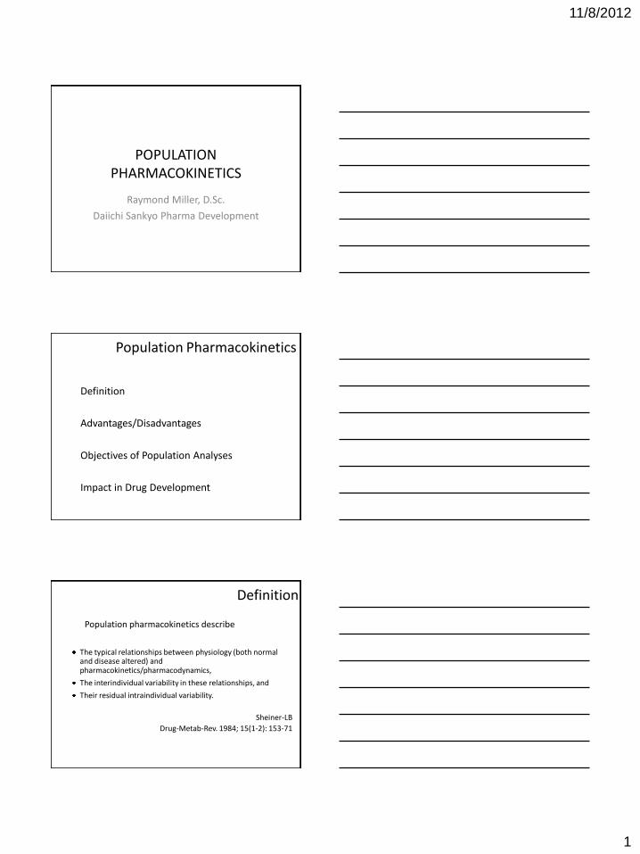
POPULATION PHARMACOKINETICS

Raymond Miller, D.Sc.

Daiichi Sankyo Pharma Development

Population Pharmacokinetics

Definition

Advantages/Disadvantages

Objectives of Population Analyses

Impact in Drug Development

Population pharmacokinetics describe

The typical relationships between physiology (both normal and disease altered) and pharmacokinetics/pharmacodynamics,

The interindividual variability in these relationships, and

Their residual intraindividual variability.

Sheiner-LB

Drug-Metab-Rev. 1984; 15(1-2): 153-71

Definition

11/8/2012

2

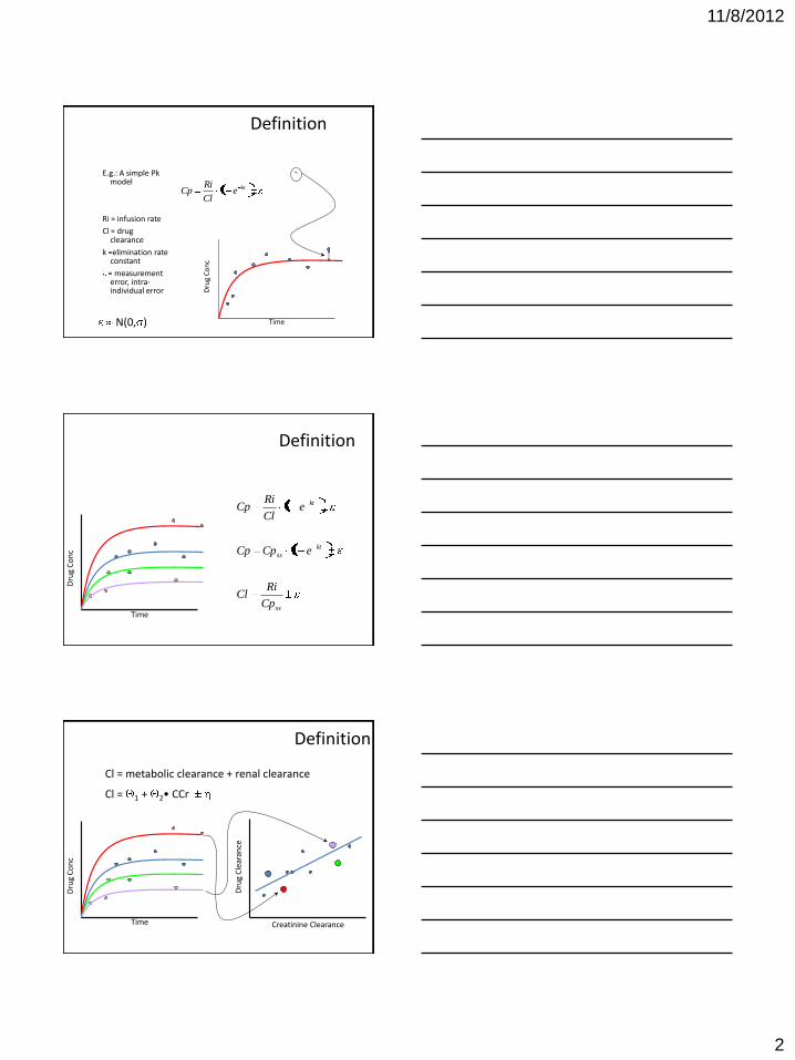
Definition

E.g.: A simple Pk model

Ri = infusion rate

Cl = drug clearance

k =elimination rate constant

= measurement error, intra-individual error D

rug

Co

nc

Time N(0, )

kteCl

RiCp 1

Definition

Dru

g C

on

c

Time ss

kt

ss

kt

Cp

RiCl

eCpCp

eCl

RiCp

1

1

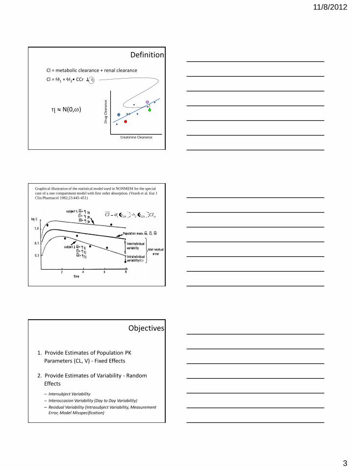
Cl = metabolic clearance + renal clearance

Cl = 1 + 2• CCr

Dru

g C

lear

ance

Creatinine Clearance

Dru

g C

on

c

Time

Definition

11/8/2012

3

Cl = metabolic clearance + renal clearance

Cl = 1 + 2• CCr

Dru

g C

lear

ance

Creatinine Clearance

N(0, )

Definition

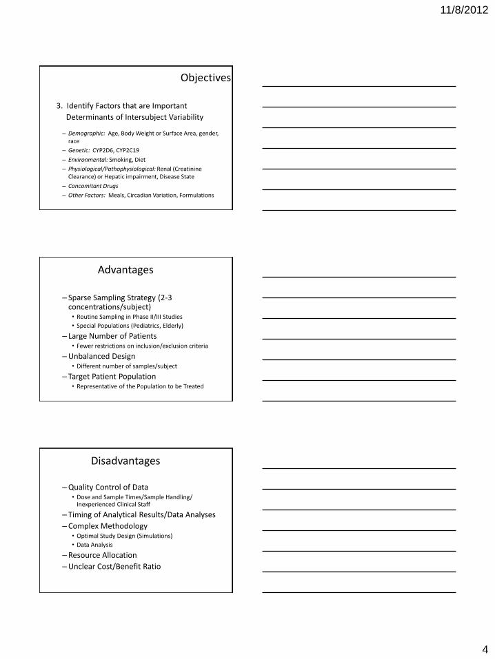
Graphical illustration of the statistical model used in NONMEM for the special

case of a one compartment model with first order absorption. (Vozeh et al. Eur J

Clin Pharmacol 1982;23:445-451)

crkk ClCl 222211

Objectives

1. Provide Estimates of Population PK

Parameters (CL, V) - Fixed Effects

2. Provide Estimates of Variability - Random

Effects – Intersubject Variability

– Interoccasion Variability (Day to Day Variability)

– Residual Variability (Intrasubject Variability, Measurement Error, Model Misspecification)

11/8/2012

4

Objectives

3. Identify Factors that are Important

Determinants of Intersubject Variability

– Demographic: Age, Body Weight or Surface Area, gender, race

– Genetic: CYP2D6, CYP2C19

– Environmental: Smoking, Diet

– Physiological/Pathophysiological: Renal (Creatinine Clearance) or Hepatic impairment, Disease State

– Concomitant Drugs

– Other Factors: Meals, Circadian Variation, Formulations

Advantages

– Sparse Sampling Strategy (2-3 concentrations/subject) • Routine Sampling in Phase II/III Studies

• Special Populations (Pediatrics, Elderly)

– Large Number of Patients • Fewer restrictions on inclusion/exclusion criteria

– Unbalanced Design • Different number of samples/subject

– Target Patient Population • Representative of the Population to be Treated

Disadvantages

– Quality Control of Data • Dose and Sample Times/Sample Handling/

Inexperienced Clinical Staff

– Timing of Analytical Results/Data Analyses

– Complex Methodology • Optimal Study Design (Simulations)

• Data Analysis

– Resource Allocation

– Unclear Cost/Benefit Ratio

11/8/2012

5

Dru

g C

on

c

Time

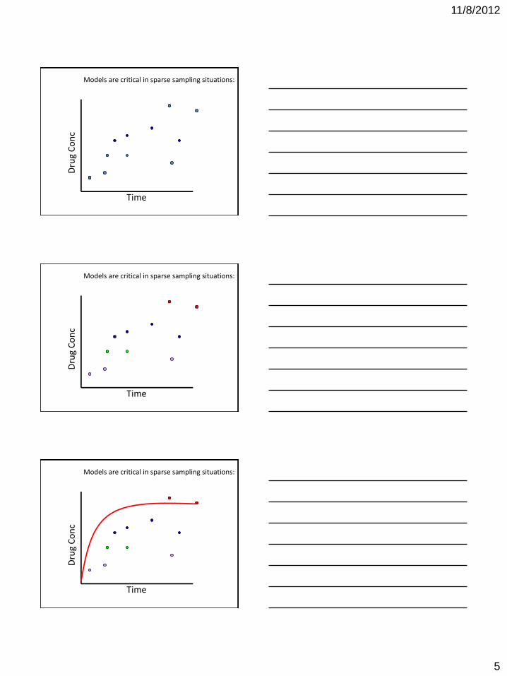
Models are critical in sparse sampling situations: D

rug

Co

nc

Time

Models are critical in sparse sampling situations:

Dru

g C

on

c

Time

Models are critical in sparse sampling situations:

11/8/2012

6

Dru

g C

on

c

Time

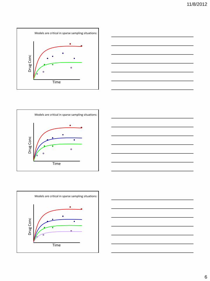
Models are critical in sparse sampling situations: D

rug

Co

nc

Time

Models are critical in sparse sampling situations:

Dru

g C

on

c

Time

Models are critical in sparse sampling situations:

11/8/2012

7

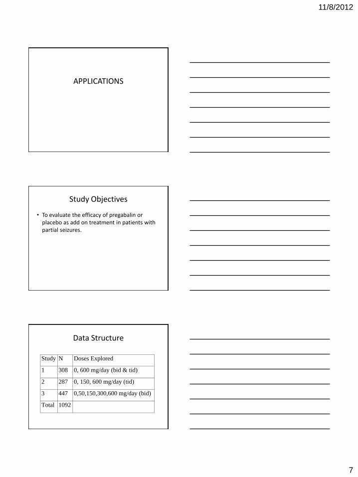
APPLICATIONS

Study Objectives

• To evaluate the efficacy of pregabalin or placebo as add on treatment in patients with partial seizures.

Data Structure

Study N Doses Explored

1 308 0, 600 mg/day (bid & tid)

2 287 0, 150, 600 mg/day (tid)

3 447 0,50,150,300,600 mg/day (bid)

Total 1092

11/8/2012

8

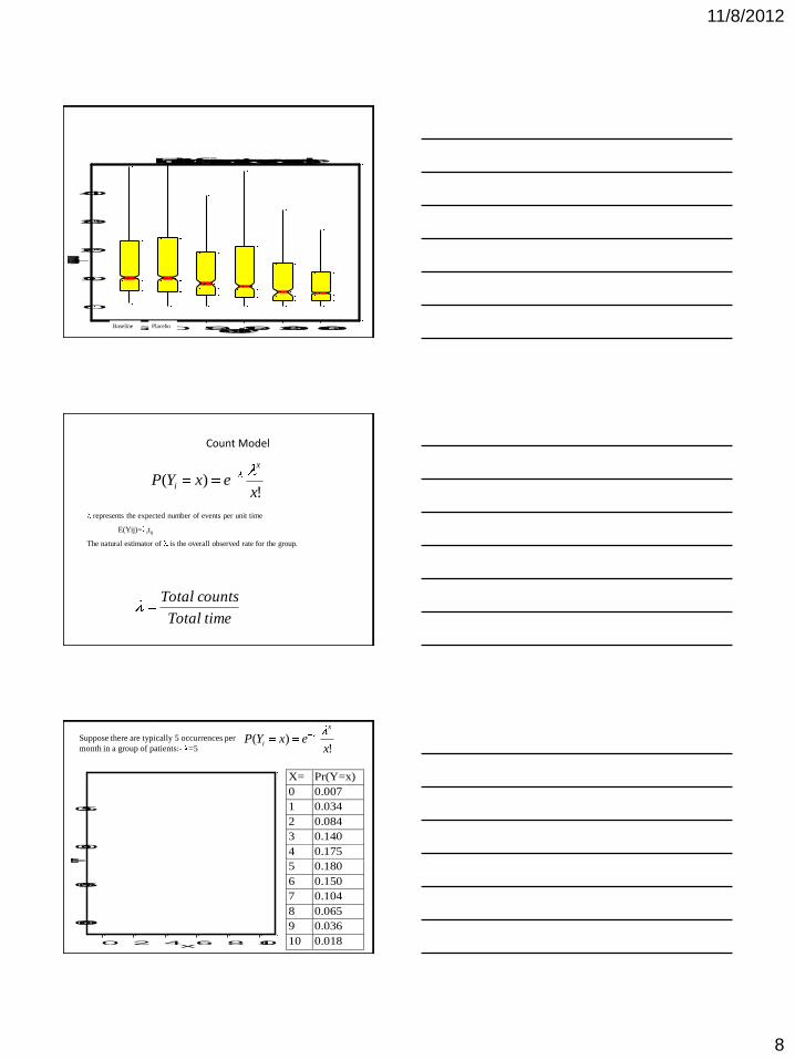
-50 0 50 150300600dose

0

10

20

30

40

Seizures per month

Boxplot of seizure rate versus dose

Baseline Placebo

Count Model

!)(

xexYP

x

i

represents the expected number of events per unit time

E(Yij)= itij

The natural estimator of is the overall observed rate for the group.

timeTotal

countsTotal

0 2 4 6 8 10x

0.00

0.05

0.10

0.15

Pr(Yi=x)

X= Pr(Y=x)

0 0.007

1 0.034

2 0.084

3 0.140

4 0.175

5 0.180

6 0.150

7 0.104

8 0.065

9 0.036

10 0.0189

!)(

xexYP

x

iSuppose there are typically 5 occurrences per

month in a group of patients:- =5

11/8/2012

9

!)(

xexYP

x

i

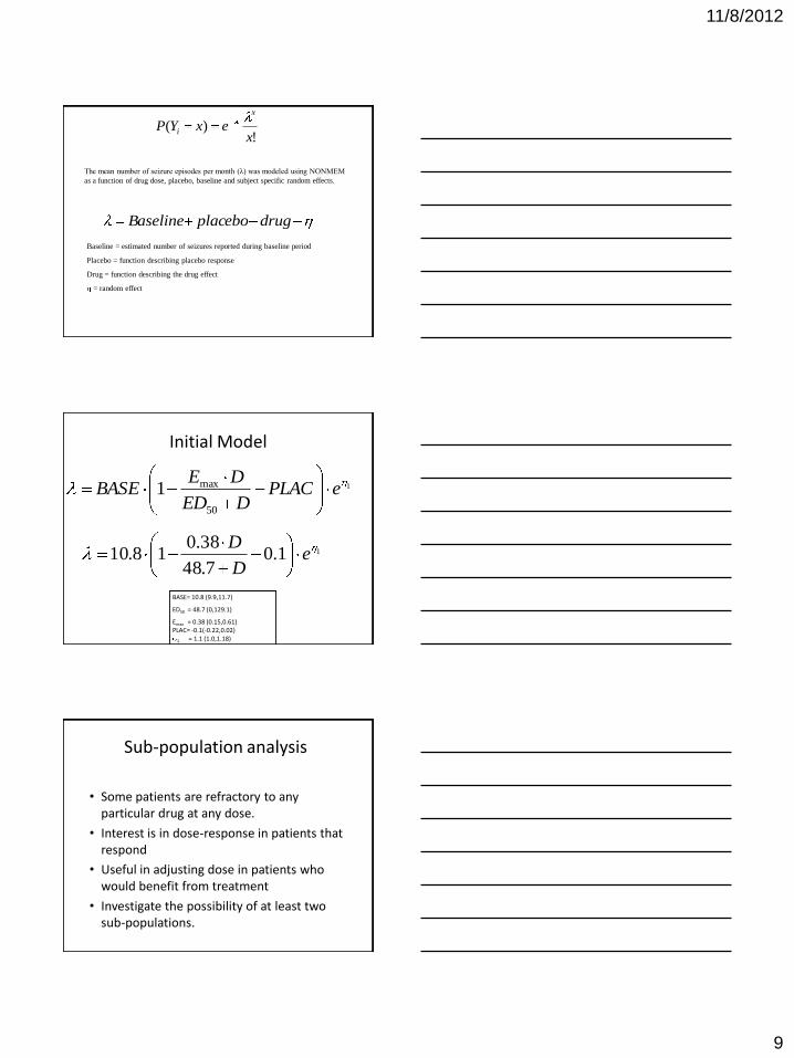
The mean number of seizure episodes per month (λ) was modeled using NONMEM

as a function of drug dose, placebo, baseline and subject specific random effects.

drugplaceboBaseline

Baseline = estimated number of seizures reported during baseline period

Placebo = function describing placebo response

Drug = function describing the drug effect

= random effect

1

50

max1 ePLACDED

DEBASE

BASE= 10.8 (9.9,11.7)

ED50 = 48.7 (0,129.1)

Emax = 0.38 (0.15,0.61) PLAC= -0.1(-0.22,0.02)

1 = 1.1 (1.0,1.18)

11.07.48

38.018.10 e

D

D

Initial Model

Sub-population analysis

• Some patients are refractory to any particular drug at any dose.

• Interest is in dose-response in patients that respond

• Useful in adjusting dose in patients who would benefit from treatment

• Investigate the possibility of at least two sub-populations.

11/8/2012

10

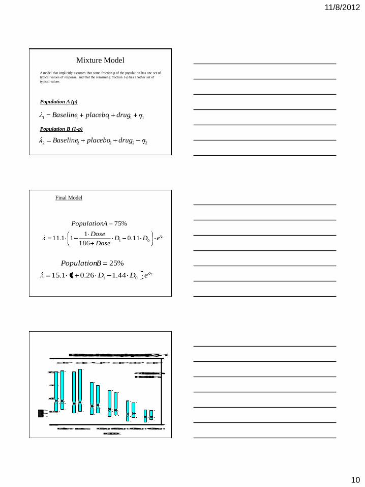
11111 drugplaceboBaseline

22222 drugplaceboBaseline

Population A (p)

Population B (1-p)

Mixture Model

A model that implicitly assumes that some fraction p of the population has one set of

typical values of response, and that the remaining fraction 1-p has another set of

typical values

1

01 11.0186

111.11

%75

eDDDose

Dose

APopulation

Final Model

2

01 44.126.011.15

%25

eDD

BPopulation

DOSE

0

5

10

15

20

Monthly Seizure Frequency (median and quartiles)

BaselinePlacebo 50 mg150 mg300 mg600 mg

PO O O OO OP P P P P

O=Observation

P=Prediction

O

Patients demonstrating dose-response (75%)

11/8/2012

11

DOSE

0

30

60

90

Monthly Seizure Frequency (median and quartiles)

Patients not demonstrating dose-response (25%)

BaselinePlacebo50 mg150 mg300 mg600 mg

PP PPPPO OO O O O

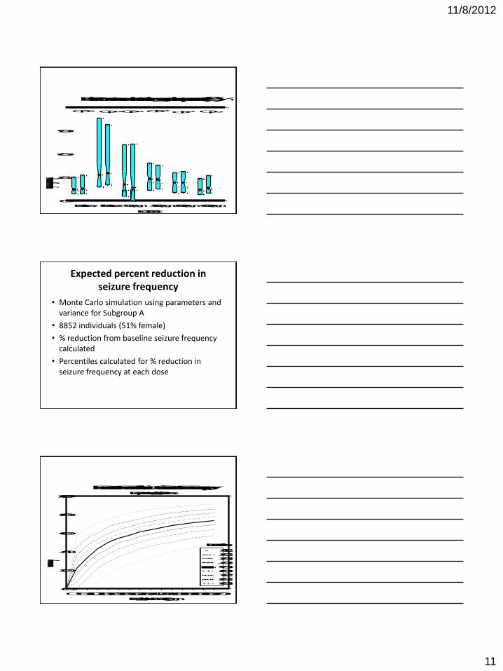
Expected percent reduction in seizure frequency

• Monte Carlo simulation using parameters and variance for Subgroup A

• 8852 individuals (51% female)

• % reduction from baseline seizure frequency calculated

• Percentiles calculated for % reduction in seizure frequency at each dose

050100150200250300350400450500550600650700

Pregabalin Dose (mg)

0

20

40

60

80

100

% Reduction in Seizure Frequency

10%

20%

30%

40%

50%

60%

70%

80%

90%

Percent Reduction in Seizure FrequencyResponding Patients

Percentile

11/8/2012

12

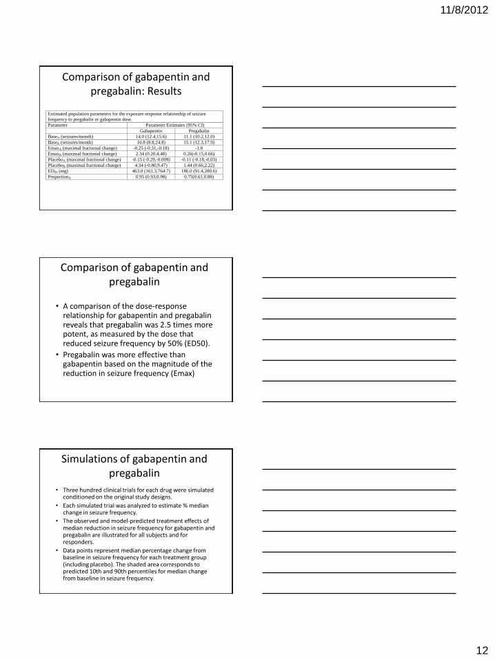
Comparison of gabapentin and pregabalin: Results

Estimated population parameters for the exposure-response relationship of seizure

frequency to pregabalin or gabapentin dose.

Parameter Parameter Estimates (95% CI)

Gabapentin Pregabalin

BaseA (seizures/month) 14.0 (12.4,15.6) 11.1 (10.2,12.0)

BaseB (seizures/month) 16.8 (8.8,24.8) 15.1 (12.3,17.9)

EmaxA (maximal fractional change) -0.25 (-0.31,-0.18) -1.0

EmaxB (maximal fractional change) 2.34 (0.20,4.48) 0.26(-0.15,0.66)

PlaceboA (maximal fractional change) -0.15 (-0.29,-0.009) -0.11 (-0.18,-0.03)

PlaceboB (maximal fractional change) 4.34 (-0.80,9.47) 1.44 (0.66,2.22)

ED50 (mg) 463.0 (161.3,764.7) 186.0 (91.4,280.6)

ProportionA 0.95 (0.93,0.98) 0.75(0.61,0.88)

Comparison of gabapentin and pregabalin

• A comparison of the dose-response relationship for gabapentin and pregabalin reveals that pregabalin was 2.5 times more potent, as measured by the dose that reduced seizure frequency by 50% (ED50).

• Pregabalin was more effective than gabapentin based on the magnitude of the reduction in seizure frequency (Emax)

Simulations of gabapentin and pregabalin

• Three hundred clinical trials for each drug were simulated conditioned on the original study designs.

• Each simulated trial was analyzed to estimate % median change in seizure frequency.

• The observed and model-predicted treatment effects of median reduction in seizure frequency for gabapentin and pregabalin are illustrated for all subjects and for responders.

• Data points represent median percentage change from baseline in seizure frequency for each treatment group (including placebo). The shaded area corresponds to predicted 10th and 90th percentiles for median change from baseline in seizure frequency.

11/8/2012

13

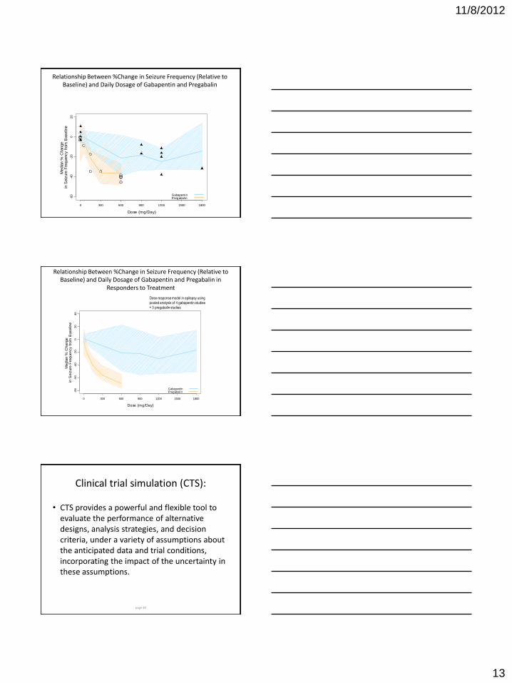
Relationship Between %Change in Seizure Frequency (Relative to Baseline) and Daily Dosage of Gabapentin and Pregabalin

• Dose-response model in

epilepsy using pooled

analysis of 4 gabapentin

studies + 3 pregabalin

studies

Dose (mg/Day)

Media

n %

Change

in S

eiz

ure

Fre

quency f

rom

Baselin

e

0 300 600 900 1200 1500 1800

-60

-40

-20

020

GabapentinPregabalin

Relationship Between %Change in Seizure Frequency (Relative to Baseline) and Daily Dosage of Gabapentin and Pregabalin in

Responders to Treatment

Dose (mg/Day)

Media

n %

Change

in S

eiz

ure

Fre

quency f

rom

Baselin

e

0 300 600 900 1200 1500 1800

-80

-60

-40

-20

020

40

GabapentinPregabalin

Dose-response model in epilepsy using

pooled analysis of 4 gabapentin studies

+ 3 pregabalin studies

Clinical trial simulation (CTS):

• CTS provides a powerful and flexible tool to evaluate the performance of alternative designs, analysis strategies, and decision criteria, under a variety of assumptions about the anticipated data and trial conditions, incorporating the impact of the uncertainty in these assumptions.

page 39

11/8/2012

14

40

CTS Procedure

Simulate i

i ~ N(3.27, 0.62)

Simulate Data

Yij|i ~ N(i, 7.02)

j=1,…,n

Calculate Mean n

jijni YY

1

1

Compare Truth

vs Data-Analytic

Decision

Determine

Correct Decision

Go: i 3

No Go: i<3

Apply

Decision Rule

33

i

iY

Y :Go No

:Go

Calculate Metrics

P(Go)

P(correct)

i>N Repeat for

i = 1,…,N

trials

i N

41

Mean Model Example Results – n=100

Decision

Truth No Go ( <3) Go ( 3) Total

i<3 2277

22.77%

989

9.89%

3266

32.66%

i 3 1598

15.98%

5136

51.36%

6734

67.34%

Total 3875

38.75%

6125

61.25%

10,000

100%

iY iY

P(Go) = 61.25%

P(correct) = 22.77% + 51.36% = 74.13%

Example: Type 2 diabetes

page 42

MAD Study Design Model-Based Evaluation

Clinical team wanted to do a short phase 1

study to estimate robustness to predict long

term outcome in type 2 diabetic patients.

11/8/2012

15

Question

• Can a 2 wk or 4 wk MAD study in T2DM provide enough data to robustly predict the long-term, i.e. 16wk, efficacy and safety?

– Fasting plasma glucose (FPG), HbA1c and risk of edema

• Early Go/No-go decision

• Guide dose-selection for PoC study

page 43

Prior in-house knowledge

• Rivoglitazone (PPARγ agonist)

• PK/PD model describing longitudinal relationship between Rivoglitazone exposure and FPG, HbA1c, and risk of edema)

page 44

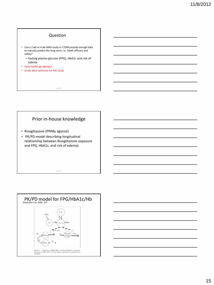
PK/PD model for FPG/HbA1c/Hb

page 45

Shashank et al, 2008, JCP

11/8/2012

16

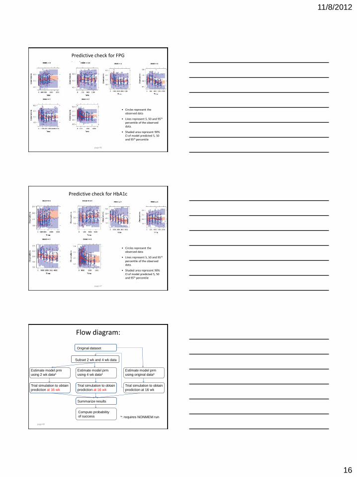
Predictive check for FPG

page 46

• Circles represent the observed data

• Lines represent 5, 50 and 95th percentile of the observed data.

• Shaded area represent 90% CI of model predicted 5, 50 and 95th percentile

Predictive check for HbA1c

page 47

• Circles represent the observed data

• Lines represent 5, 50 and 95th percentile of the observed data.

• Shaded area represent 90% CI of model predicted 5, 50 and 95th percentile

page 48

Flow diagram:

Original dataset

Subset 2 wk and 4 wk data

Estimate model prm

using 2 wk data*

Estimate model prm

using 4 wk data*

Trial simulation to obtain

prediction at 16 wk

Trial simulation to obtain

prediction at 16 wk

Summarize results

Estimate model prm

using original data*

Trial simulation to obtain

prediction at 16 wk

Compute probability

of success

*: requires NONMEM run

11/8/2012

17

page 49

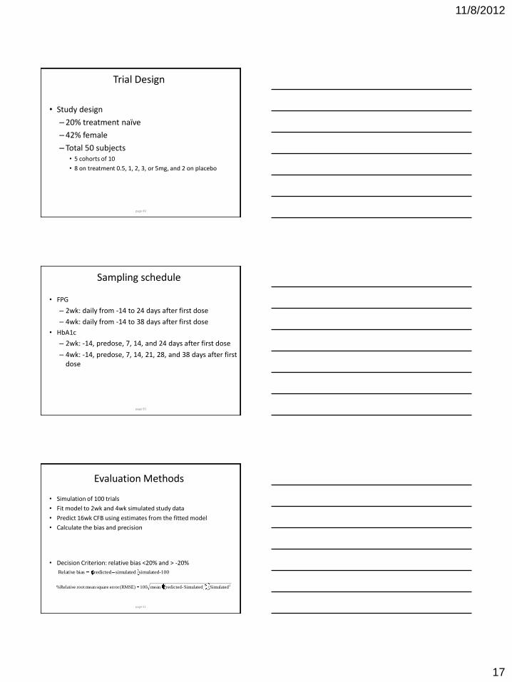
Trial Design

• Study design

– 20% treatment naïve

– 42% female

– Total 50 subjects • 5 cohorts of 10

• 8 on treatment 0.5, 1, 2, 3, or 5mg, and 2 on placebo

page 50

Sampling schedule

• FPG

– 2wk: daily from -14 to 24 days after first dose

– 4wk: daily from -14 to 38 days after first dose

• HbA1c

– 2wk: -14, predose, 7, 14, and 24 days after first dose

– 4wk: -14, predose, 7, 14, 21, 28, and 38 days after first dose

page 51

Evaluation Methods

• Simulation of 100 trials

• Fit model to 2wk and 4wk simulated study data

• Predict 16wk CFB using estimates from the fitted model

• Calculate the bias and precision

• Decision Criterion: relative bias <20% and > -20%

22Simulated/Simulated-Predictedmean100(RMSE)error squaremean root %Relative

100/simulatedsimulatedpredictedbiasRelative

11/8/2012

18

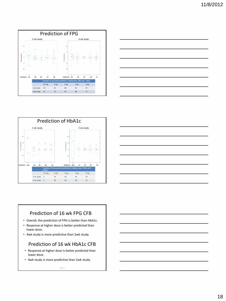
Prediction of FPG

page 52

Number of successful predictions (relative bias <20% and > -20%)

0.5 mg 1 mg 2 mg 3 mg 5 mg

2 wk study 35 55 48 55 57

4 wk study 41 73 81 80 77

2 wk study 4 wk study

RMSE% 44 28 26 27 26 RMSE% 35 18 15 16 17

Prediction of HbA1c

page 53

Number of successful predictions (relative bias <20% and > -

20%)

0.5 mg 1 mg 2 mg 3 mg 5 mg

2 wk study 3 26 46 49 53

4 wk study 6 35 60 58 61

2 wk study 4 wk study

RMSE% 384 37 24 25 25 RMSE% 461 54 36 36 32

Prediction of 16 wk FPG CFB • Overall, the prediction of FPG is better than HbA1c.

• Response at higher dose is better predicted than lower dose.

• 4wk study is more predictive than 2wk study.

page 54

Prediction of 16 wk HbA1c CFB • Response at higher dose is better predicted than

lower dose.

• 4wk study is more predictive than 2wk study.

11/8/2012

19

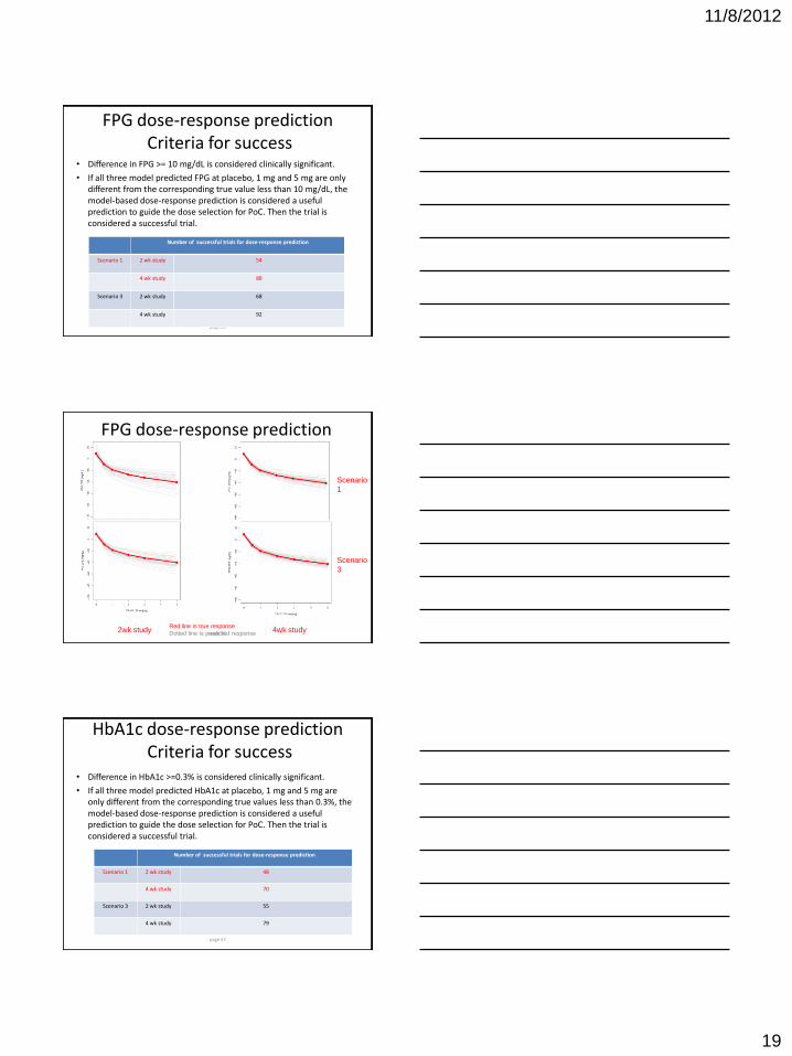
FPG dose-response prediction Criteria for success

• Difference in FPG >= 10 mg/dL is considered clinically significant.

• If all three model predicted FPG at placebo, 1 mg and 5 mg are only different from the corresponding true value less than 10 mg/dL, the model-based dose-response prediction is considered a useful prediction to guide the dose selection for PoC. Then the trial is considered a successful trial.

page 55

Number of successful trials for dose-response prediction

Scenario 1 2 wk study 54

4 wk study 88

Scenario 3 2 wk study 68

4 wk study 92

FPG dose-response prediction

page 56 2wk study 4wk study Red line is true response

Dotted line is predicted response

Scenario

1

Scenario

3

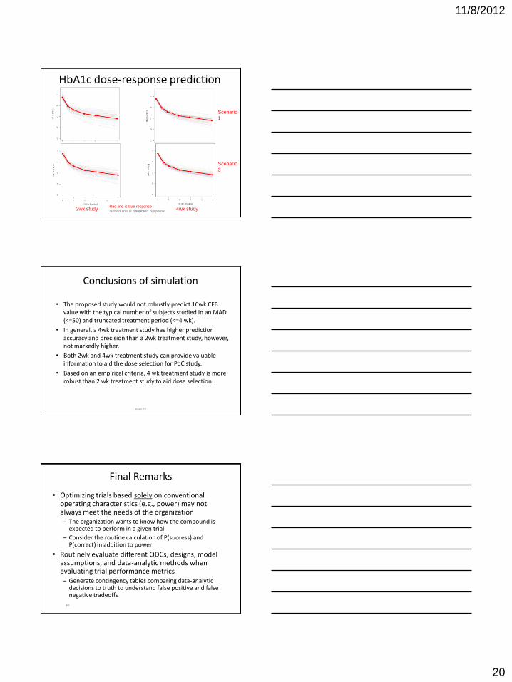
HbA1c dose-response prediction Criteria for success

• Difference in HbA1c >=0.3% is considered clinically significant.

• If all three model predicted HbA1c at placebo, 1 mg and 5 mg are only different from the corresponding true values less than 0.3%, the model-based dose-response prediction is considered a useful prediction to guide the dose selection for PoC. Then the trial is considered a successful trial.

page 57

Number of successful trials for dose-response prediction

Scenario 1 2 wk study 48

4 wk study 70

Scenario 3 2 wk study 55

4 wk study 79

11/8/2012

20

HbA1c dose-response prediction

page 58 2wk study 4wk study Red line is true response

Dotted line is predicted response

Scenario

1

Scenario

3

Conclusions of simulation

• The proposed study would not robustly predict 16wk CFB value with the typical number of subjects studied in an MAD (<=50) and truncated treatment period (<=4 wk).

• In general, a 4wk treatment study has higher prediction accuracy and precision than a 2wk treatment study, however, not markedly higher.

• Both 2wk and 4wk treatment study can provide valuable information to aid the dose selection for PoC study.

• Based on an empirical criteria, 4 wk treatment study is more robust than 2 wk treatment study to aid dose selection.

page 59

60

Final Remarks

• Optimizing trials based solely on conventional operating characteristics (e.g., power) may not always meet the needs of the organization – The organization wants to know how the compound is

expected to perform in a given trial

– Consider the routine calculation of P(success) and P(correct) in addition to power

• Routinely evaluate different QDCs, designs, model assumptions, and data-analytic methods when evaluating trial performance metrics – Generate contingency tables comparing data-analytic

decisions to truth to understand false positive and false negative tradeoffs

11/8/2012

21

61

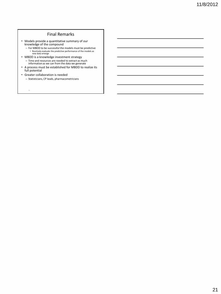
Final Remarks

• Models provide a quantitative summary of our knowledge of the compound – For MBDD to be successful the models must be predictive

• Routinely evaluate the predictive performance of the models as new data emerge

• MBDD is a knowledge investment strategy – Time and resources are needed to extract as much

information as we can from the data we generate

• A process must be established for MBDD to realize its full potential

• Greater collaboration is needed – Statisticians, CP leads, pharmacometricians