Political Attitudes toward the Environment: The …polisci.ucsd.edu/_files/undergrad/Thesis 2013 Political Attitudes...i Political Attitudes toward the Environment: The Politics of

i

Political Attitudes toward the Environment: The

Politics of Residential Solar Panel Installations in

California

Samson Yuchi Mai

A Senior Honors Thesis Submitted to the Department of Political

Science, University of California San Diego

April 1, 2013

ii

To my loving mother, father, little brother, and relatives.

To family.

To friends.

iii

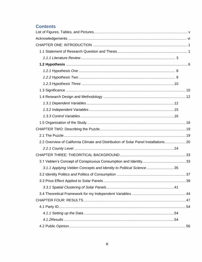
Contents List of Figures, Tables, and Pictures ........................................................................................... v

Acknowledgements ................................................................................................................... vi

CHAPTER ONE: INTRODUCTION ............................................................................................ 1

1.1 Statement of Research Question and Thesis .................................................................... 1

1.1.1 Literature Review ............................................................................................ 3

1.2 Hypothesis ...................................................................................................................... 6

1.2.1 Hypothesis One .............................................................................................. 8

1.2.2 Hypothesis Two .............................................................................................. 9

1.2.3 Hypothesis Three ..........................................................................................10

1.3 Significance .................................................................................................................... 10

1.4 Research Design and Methodology ................................................................................ 12

1.3.1 Dependent Variables .....................................................................................12

1.3.2 Independent Variables ...................................................................................15

1.3.3 Control Variables ...........................................................................................16

1.5 Organization of the Study ................................................................................................ 16

CHAPTER TWO: Describing the Puzzle ................................................................................... 19

2.1 The Puzzle ...................................................................................................................... 19

2.2 Overview of California Climate and Distribution of Solar Panel Installations .................... 20

2.2.1 County Level .................................................................................................24

CHAPTER THREE: THEORITICAL BACKGROUND ................................................................ 33

3.1 Veblen’s Concept of Conspicuous Consumption and Identity .......................................... 33

3.1.1 Applying Veblen Concepts and Identity to Political Science ...........................35

3.2 Identity Politics and Politics of Consumption ................................................................... 37

3.3 Prius Effect Applied to Solar Panels ................................................................................ 39

3.3.1 Spatial Clustering of Solar Panels..................................................................41

3.4 Theoretical Framework for my Independent Variables .................................................... 44

CHAPTER FOUR: RESULTS ................................................................................................... 47

4.1 Party ID ........................................................................................................................... 54

4.1.1 Setting up the Data ........................................................................................54

4.1.2Results ...........................................................................................................54

4.2 Public Opinion ................................................................................................................. 56

iv


4.2.2 Results ..........................................................................................................58

4.3 Voting Patterns ............................................................................................................... 58


4.3.2 Results ..........................................................................................................60

CHAPTER FIVE: CONCLUSION .............................................................................................. 61

5.1 Findings .......................................................................................................................... 61

5.2 Flaws in my Research Design ......................................................................................... 62

5.3 Creating an Ideal Research Design and Research Study ................................................ 64

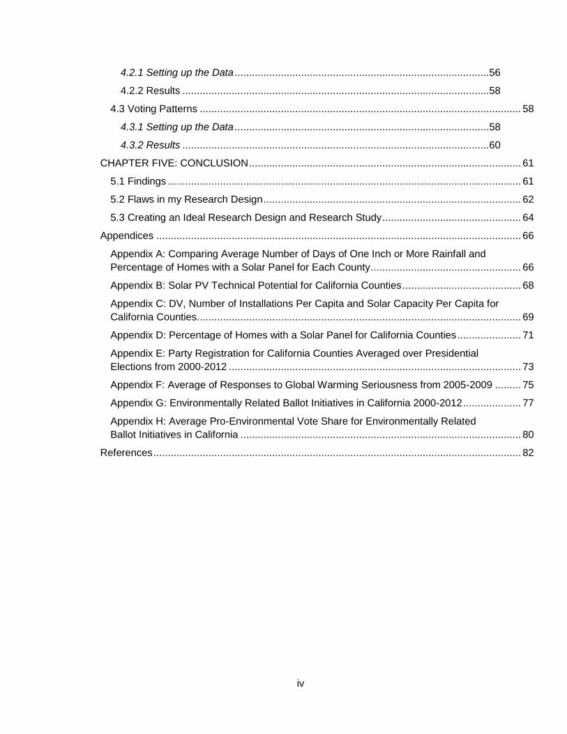
Appendices .............................................................................................................................. 66

Appendix A: Comparing Average Number of Days of One Inch or More Rainfall and

Percentage of Homes with a Solar Panel for Each County .................................................... 66

Appendix B: Solar PV Technical Potential for California Counties ......................................... 68

Appendix C: DV, Number of Installations Per Capita and Solar Capacity Per Capita for

California Counties ................................................................................................................ 69

Appendix D: Percentage of Homes with a Solar Panel for California Counties ...................... 71

Appendix E: Party Registration for California Counties Averaged over Presidential

Elections from 2000-2012 ..................................................................................................... 73

Appendix F: Average of Responses to Global Warming Seriousness from 2005-2009 ......... 75

Appendix G: Environmentally Related Ballot Initiatives in California 2000-2012 .................... 77

Appendix H: Average Pro-Environmental Vote Share for Environmentally Related

Ballot Initiatives in California ................................................................................................. 80

References ............................................................................................................................... 82

v

List of Figures and Tables

Figure 1: Actual vs. Potential Solar Residential Capacity to 2016 P. 14 Figure 2: Solar Radiation in the California measured in kW*hours/meters squared per day P. 21 Figure 3: Map of California Counties’ Solar Power Generating Potential P. 22 Figure 4: Heat Map of Solar Installations throughout California Prior to Q3 2011 P. 24 Figure 5: Relationship between Percentage of Homes with a Solar Panel and Number of Days of Rainfall of One Inch or More for California Counties P. 26 Figure 6: Relationship Between Percentage of Homes with a Solar Panel and Solar Power Generating Potential Measured in MWH per day P. 31 Figure 7: Prius Ownership and Obama Vote Share 2008 Election in Washington (1 dot represents 5 Priuses) P. 42 Figure 8: Clustering of Solar PV Panels in the Bay Area P. 44 Figure 9: Linear Regression of Democratic Registration and Number of Solar Panel Installations Per Capita P. 49 Table 1: Descriptive Statistics of “Relationship Between Percentage of Homes with a Solar Panel and Number of Days of Rainfall of One Inch or More for California Counties” Scatterplot P. 26 Table 2: Descriptive Statistics of “Relationship between Percentage of Homes with a Solar Panel and Solar Power Generating Potential Measured in MWH per day” P. 31 Table 3: Summary of Linear Regression Models without Control Variables P. 49 Table 4: Summary of Linear Regression Models with Control Variables P. 51 Table 5: Regression Coefficients of the Control Variables and Solar Power Capacity Per Capita P. 53 Table 6: Regression Model Summary of Democratic Registration and Number of Solar Panel Installations Per Capita P. 55 Table 7: California State Ballot Initiatives that Dealt with Environmental Issues 2000-2012 P. 59

vi

Acknowledgements

I would like first thank my faculty advisor, Professor Broz for the time and

effort he has put in guiding me through this long process. I learned a lot and will

cherish the academic rigor that was instilled in me throughout the whole process

and for the rest of my life. Two of the most important skills that I learned from the

honors seminar were learning how to think about and write about complex

issues.

My friends deserve a special thank you especially those who helped me

on this thesis. When I hit an obstacle, you will there with me to help me

overcome it. I must give special thanks to Arik Burakovsky, Jonathan Chu,

Harrison Gill, Christina Halstead, and Kenneth Cummings. I also want to thank

my peers in the political science honors seminar for their help as well.

I also want to acknowledge my parents, my little brother, my grandparents,

my aunts and uncles, cousins, and other relatives that supported me. I would not

be where I am today without their love and care. And for that, I am thankful.

1

CHAPTER ONE: INTRODUCTION

1.1 Statement of Research Question and Thesis

My thesis seeks to understand why the use of residential solar power

varies across California counties. The pattern of usage does not match solar

power generating potential. Solar power generating potential is the maximum

amount of energy that can be generated from residential solar panels. A county

that has more days of sunshine per year has higher solar power generating

potential. However, climate does not do a sufficient job of explaining the

distribution of solar panel installations throughout the state of California. For

example, there tends to be more residential solar power usage in northern and

coastal counties than in sunnier inland countries. My argument is that residents

install solar panels primarily for non-economic political and social reasons, and

that pecuniary gains of solar power are of secondary importance to homeowners’

decision to install solar panels.

My theoretical framework on explaining the puzzle rests on expanding the

definition of politics of identity and overlapping it with economics. I delineate the

decision of buying a solar panel as a political decision. The high economics costs

of buying and installing a solar panel makes the decision a political one. All forms

of politics “involves making comparisons and choices among- and commitments

to –values and interests and groups and individuals.” (54 Parker) The choices a

person make in the political arena is way to identify him or her. The decision to

2

buy a solar panel tells others in his or her social network that he or she is an

environmentally conscious person. My theory is that the variances of solar panel

installations per capita across California counties are based on the residents’

political and environmental attitudes.

I examine three dependent variables: the number of solar system panel

installations per person in the California county, solar capacity (kW) per person in

the California county, and the percent of homes with solar in the California

county. All three variables are similar in the sense that all three variables are

outcomes. There is an interesting discrepancy in the distribution of solar panel

installations throughout the state of California. One would expect counties with

more days of sunshine per year to have more solar panels per resident, more

solar capacity per resident, and a greater percentage of homes with solar panels.

The reason for this is more sunshine translates into more energy production. The

extra energy generated can be sold to other customers in the electricity grid to

earn credit that can be rolled into the next utility bill to reduce the utility bill or to

recuperate the costs for the investment (Cite). There is a financial disincentive for

residents of California counties with less sunshine to buy a solar panel. These

counties are concentrated in Northern California and along the coast. However,

these are the counties that have the highest percentages of solar outcomes per

person.

I argue person’s political and environmental beliefs and values will be the

overriding consideration in a person’s decision to purchase a solar panel for their

3

home. That decision affirms the person’s identity to both him/herself and to the

community at large. There is research that certifies this trend for other consumer

goods.

1.1.1 Literature Review

Buying a solar panel is synonymous with being green. Another well-known

product that is also known for being synonymous with being green is the hybrid

automobile. The question was whether environmental ideology was a

determining element in the consumer choice of vehicle?

Matthew Kahn sought to find out in statistical analysis of drivers across the

state of California in his paper, Do Greens drive Hummers or hybrids?

Environmental ideology as a determinant of consumer choice in the Journal of

Environmental Economics and Management. The test was to see if

“environmentalists” make private consumer choices that reflect their belief

system which is to “live a less resource intensive lifestyle.” (1 Kahn) He admitted

that there is a possibility of free-riding from the rational thinking of process. A

person could think that his or her action would have a negligible impact on the

environmental quality because the actions of one person will make no difference

in improving the environmental situation of the community.

In examination, he found that California environmentalists did make

private choices that reflect their ecofriendly philosophy. He found that

environmentalists in California “are more likely to use public transit, consume

4

less gasoline and purchase green vehicles such as hybrids.” (16 Kahn) He also

found evidence of consumer heterogeneity. The evidence suggest there is a

possibility of social interaction that could lead environmentalists to make

consumer decisions such as buying a hybrid car to highlight their “greenness” to

their peers in the same community.

If environmental and political ideology is a determinant for transportation

choices, could it apply to residential solar panels as well? Our claims are similar.

He argues that environmental ideology is a determent of transportation choice. I

argue that environmental and political beliefs are a determinant of the decision of

whether or not to purchase a solar panel. Kahn’s geographical area of analysis

was across the state of California. My area of analysis is also California.

And both products share similar characteristics. Both hybrid vehicles and

solar panel are expensive investment costing thousands of dollars each. A hybrid

car requires at least several years to break even. In the case of a Toyota Prius

Hybrid, it takes an average of 9-10 years.1 If you compared hybrids to their

counterparts in the same class of economy cars, they are 25 % to 30% more

expensive (Bradford). The break-even point for solar panels is even longer in

comparison to the time it takes for a hybrid to break even. Even with all the tax

credits and rebates, the costs of installing a solar panel are still quite high. In

New Jersey, an above average electricity user of $100 a month can purchase a

1 At an average of $4/gallon, you would break even after 124,000 miles from the Consumer Guide

Automotive. The average American drives 13,476 miles a year according to the Federal Highway Administration. So that translates to a break-even point of approximately 9.2 years.

5

solar system at $54,000. Including state rebate of $18, 468 and a $2,000 federal

tax credit, the system costs are reduced to $33,532. The break-even point for this

system is 11 to 22 years (Darlin). The average break-point for a solar panel in

California is 14 years as stated by Polly Shaw, a senior regulatory analyst at the

California Public Utilities Commission (Darlin). The motivation to purchase a

hybrid car or a solar panel is not economic as indicated by John Anderson, a

senior principal at the Rocky Mountain Institute, an energy research and

consultancy firm (Darlin). This implies that some other incentive is the driving

force for people to purchase solar panels.

There is evidence that political and environmental beliefs are the

determinant for the purchase and installations of solar panels in California.

Samuel Dastrup, Joshua Graff Zivin, Dora Costa, and Matthew Kahn in

Understanding the Solar Home Price Premium: Electricity Generation and

“Green” Social Status wanted to find out if there was market capitalization effect

from installing solar panels in San Diego and Sacramento counties. Market

capitalization effect means the premium the homeowner gains when they sell his

or her home. They found little evidence of a market capitalization effect. It was

estimated to be three to four percent premium (17 Dastrup). They did find

another fascinating condition. They found the premium to larger in communities

with more Prius autos and neighborhoods with more college graduates (17

Dastrup). More significantly, they found a positive relationship between market

capitalization effect and Green party registration and Democratic registration (13

6

Dastrup). They also observed a positive relationship between market

capitalization and median income and education.

This is evidence that suggest there is a possibility of a connection

between political and environmental philosophy and the percentage of solar

panel and solar capacity in a California county. There is evidence of the

relationship existing in San Diego and Sacramento counties. The results in

Dastrup et al.’s study mirror some of the results found in Kahn’s research piece.

Both found a positive correlation between percentage of registered Democrats

and Greens in a county and their dependent variable. Dastrup ET. Al. viewed

political identification as a predicator of the capitalization effects of solar panels. I

view political and environmental beliefs which include political identification as a

determinant of the decision to purchase a solar panel. My thesis mirrors Kahn’s

analysis between transportation choices and environmental values in California. I

will do the same, but my dependent variable will be solar panels per capita

instead of mode of transportation.

1.2 Hypothesis

My theory is that political ideology shapes Californian’s decision to

purchase an energy generating solar system for their property. A person’s

political ideology is a unified set of beliefs. These set of attitudes are based on a

set of values which are socialized by the surroundings, social networks, and

reinforcing behavior. In the case of my study, I focus on environmentalists

7

whose overall mission is conservation and mitigating the effects of human

actions on global society and on the ecosystem. I take a similar supposition

made by Kahn (2003). He assumes that environmentalists will make consistent

choices in both the public sphere which is displayed in the ballot box and through

self-identification, as well in private consumer decision-making. In both the

private and public sphere, the environmentalist will make choices that will

minimize his or her impact on the ecosystem and human society. That means

making choices that will use fewer natural resources, pollute less, and produce

less carbon emissions. The decision to purchase a solar panel will consistently

reflect the environmental political philosophy.

My goal is to quantify these environmental and political attitudes and

measure how much these attitudes affect Californian’s decision-making on the

purchase of photovoltaic panels for their homes. I have come up with three

separate measures to identify whether or not a person is environmentally

conscious or not. I will talk more of these measures later on. My overall thesis

tests the three following hypothesis:

Hypothesis 1: Counties with a greater percentage of registered Democrats and

Green party members are more likely to have a higher percentage of homes with

solar panels, greater solar capacity per resident and greater number of solar

panels per person.

8

Hypothesis 2: Counties that votes on average more in favor of pro-environment

voter ballot initiatives are more likely to have a higher percentage of homes with

solar panels, greater solar capacity per resident and greater number of solar

panels per person.

Hypothesis 3: Counties that show more concern for environmental issues are

more likely to have a higher percentage of homes with solar panels, greater solar

capacity per resident and greater number of solar panels per person.

I will expand on these three hypotheses for the rest of Section 2 of this chapter.

1.2.1 Hypothesis One

My first hypothesis is if a person is a registered Democrat or a registered

Green party member, he or she is more likely to purchase a residential solar

system for his or her home. Party identification matters because it predicts

consumer behavior. The overarching emphasis on the Green Party platform is

environmentalism. Their objective is to establish a “national Green presence in

politics and policy debate.” (http://www.gp.org/about.php) Green party members

should have the highest propensity to install a solar panel on their property.

Although environmentalism is not a main precept of the Democratic platform,

Democrats tend to see environmental issues as important as economic and

social matters on a consistent basis.(Find environment in Democratic national

platform) In fact, many Democrats see a direct link between the environment, the

economy, and social concerns. Because of the high value Democrats have

http://www.gp.org/about.php

9

toward the environment, Democrats are more likely to show outward behavior

that exemplify this belief and thus are more likely to purchase a solar panel.

My specific prediction is that counties in California that have more

registered Democrats (and Green Party members) should have more solar

panels within its boundaries. As such, I predict that counties such as San

Francisco City and County, Marin County, and Santa Cruz County to have high

levels of solar panels and solar capacity per person.

1.2.2 Hypothesis Two

My second hypothesis relates directly to attitudes toward the environment.

While political party affiliation can proxy for such attitudes, there may be some

slippage between environmental beliefs and party identification. For example, a

Republican can be economically conservative but very liberal on social and

environmental issues. Therefore, party measures of environmentalism may be

rather imprecise.

To improve on this, I also construct county-level measures of

environmental attitudes. My specific hypothesis that California counties where

residents display more concern for the environment will also have more solar

panels installed on residential properties than counties where residents are less

concerned with environmental issues. For example, if a county has a large

percentage of people who believe climate change poses a real threat to well-

10

being, the county in which those residents reside will have more residential solar

panels.

1.2.3 Hypothesis Three

My final hypothesis tests this same argument but uses a direct behavioral

measure of county-level environmentalism rather than public opinion data.

Responses to a public opinion survey are subject to many types of problems,

from “framing” problems, to “cheap talk.” These problems can be avoided by

using behavioral measures that involve costly action.

In this instance, I use county votes in favor of environmental projects on

state ballot initiatives as a behavioral measure of county-level environmentalism.

Voting is costly behavior; moreover such initiatives involve raising taxes to fund

environmental projects, which suggests that voters approving these measures

are willing to pay for them. My expectation is that in counties where more voters

favor state-level environmental initiatives, residents will be more likely to install

solar panels on their homes.

1.3 Significance

People are not solely motivated by economic considerations. Individuals

make decisions including consumer purchases and investments based on their

values and beliefs. My investigation into this puzzle can be viewed as a study

into the effects of a person’s political beliefs has on consumer decision-making.

Much of the literature that looks at why people purchase solar panels is based on

11

standard consumption theory. Standard consumption theory takes a narrow view

of how people make choices in the market. It takes into consideration income

and relative prices as the two main elements of decision-making. Keeping in the

line with the theory, much of the academic literature that aims to improve the

uptake of residential solar in California and the United States focuses on the

economic aspect of the industry. Many experts advocated more tax credits, more

rebates, and more subsidies to producers.

The use of economic inducements for environmental objectives may not

fall evenly across a population when citizens hold wildly divergent political and

environmental beliefs. However, they neglect to see the social and political

aspects of the problem. What if there were non-monetary solutions in increasing

the uptake of solar panel purchases and use by residents?

The finding of this study hopes to raise additional questions to the policy

debate. Does party identification predict whether or not you install a solar panel

on your home? Does the resident’s voting behavior share a connection with their

“consumption” of solar panels? Does a person’s environmental attitude correlate

with buying and installing a solar panel? The answers to these questions may

have broader implications on public policy dealing with climate change and future

energy development policy

12

1.4 Research Design and Methodology

I will be using three measures to determine the effects of political

viewpoints:

1) Partisan identification

2) Attitudes toward the environment.

3) Behavior by voting patterns on state voter initiatives

These three measures all capture elements of the same concept: political beliefs

about the importance of the environment. The point of having three measures of

political beliefs is to affirm that the results of this study are consistent across

alternative indicators of political values.

1.3.1 Dependent Variables

As mentioned previously, I have three dependent variables which are 1)

number of solar system panel installations per person in the California county, 2)

solar capacity (kW) per person in the California county and 3) percent of homes

with solar in the California county. Although these three variables are similar they

can imply different meanings. For example, a county may have a high level of

solar capacity per person, but it may have a lower than expected number of solar

panel person. This means each solar installation is larger. Each solar panel is

larger. This may imply that the property is larger. This is more likely in less dense

areas which are suburban and rural. To illustrate another example, there may

13

many solar panel installations in a county. However, those numbers of

installations may have taken place in different time periods at the same property.

So a select faction of homeowners may be installing additional solar panels over

a long period of time. In order to see if the level of penetration of solar panels into

the residential market in the county, one needs to examine percentage of homes

with solar panels. Three different dependent measures will assist in making

distinctions like those mentioned after the statistical analysis.

I got the raw data for my first and second dependent variable data from

the Appendix I of the California’s Solar Cities 2012: Leaders in the Race toward a

Clean Energy Future generated by Environment California Research and Policy

Center. They had the number of solar installations and solar capacity of each

city. I had to find the corresponding county for each city and aggregate the

results. Then in order to get the per capita result, I divided the number of solar

installations and solar capacity for each county by the county’s population taken

from the 2010 United States Census. The numbers for percentage of homes with

solar panels for each of the counties are taken from Sunrun.com which is taken

from the California Solar Initiative program. The data was taken to May 2010.

All the data for the three dependent variables are cumulative. At first

glance, this may pose a statistical drawback. Although I am measuring the

dependent variables with independent variables gathering from an eight year

period, solar panel installations started in the state of California way before 2000.

However, the number of installations is minimal. Therefore, it is valid to discount

14

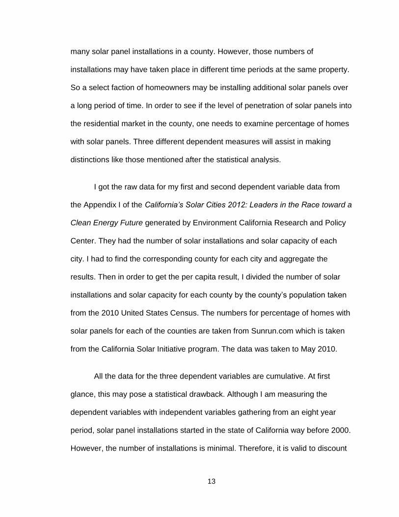
them. Moreover, the increase of solar panel installations starts in 2000 as shown

in Figure 1 below.

Figure 1: Actual vs. Potential Solar Residential Capacity to 2016

Source: Davis, Benjamin and Travis Madsen. “California’s Solar Cities 2012: Leaders in the Race toward a Clean Energy Future.” Environment California Research and Policy Center. January 2012. P.16 Print.

Admittedly, having the number of solar installations for each county on a year by

year basis will reveal how people changed their consumer behavior according to

changes in their values and beliefs measured through public opinion surveys,

voting patterns, and changes in party registration in each county. Because I have

to match the cumulative data I had for solar panel installations, percentage of

homes with solar panels, and solar capacity for each county, I had to aggregate

the data I had for my independent variables.

15

1.3.2 Independent Variables

The first independent variable is the percentage of registered Democrats,

Republicans, and Greens in each of the California counties. Political identification

is a proxy of environmental beliefs. Modern American political parties are divided

not just on economic and political issues, but on social and environmental issues

as well.

The second independent variable I will be using is the public opinions of

California residents. The public opinion of Californians on environmental issues is

taken from survey results provided by the Public Policy Institute of California.

The last independent variable in this study is the results of voter initiatives

that deal with the environment in each of the California counties. The reason why

I use this as a variable because of voting for a voter initiated proposition poses a

cost to the voter. The act of voting is a cost in itself. It takes a certain amount of

effort to research the issues and then to actually vote for your preferred choice.

On top of that, many of the state propositions stipulate increases in tax rates

and/or increased costs for the state government and taxpayers to fund the

implementation of the passed voter initiatives. Because of the associated costs, it

is possible to get a more accurate picture of the political preferences of the

residents compared to the preferences derived from a survey.

16

1.3.3 Control Variables

Although the purpose of my study is to explore the effects of political

values on microeconomic decision making on California residents, it is prudent to

look at effects of other factors. I will be using control variables to test the relative

effects of the independent variables. I stipulate that counties that have a higher

proportion of females, wealthier residents, Caucasians, and educated residents

should display more residential solar capacity. As such, my control variables will

be gender, median household income, and race.

I will also control for incentives provided for the government to install solar

panels. All homeowners in California have access to incentives provided by the

federal and state governments. I will assume that these incentives will be

constant for all California homeowners. However, there are incentives provided

by city and county governments and I will have to control for this. I will be using

data derived from the Database of State Incentives for Renewables and

Efficiency from North Carolina State University. Although this database does not

say whether or not it lists incentives by all cities and counties, it was the most

through database I came across.

1.5 Organization of the Study

My thesis contains five chapters. The first chapter of the study is my

introduction to my thesis. The chapter presents the puzzle, goes over lays out my

17

main claims, explains what my goals are, describes the methodology and

rationale of my investigation, and lays out the structure of my research.

The second chapter will delve deeper in into my research question. I will

describe in length the data behind my research question by presenting a number

of datasets, tables, and maps.

In my third chapter, I will further elaborate on the theories connected to my

research question and compare it will alternative theories of explanation.

Chapters five will cover the results of my statistical analysis. I will not talk

about every single regression I ran because many of the regressions

turned out to be statistically insignificant. The regressions that I will elaborate

on are those that are statistically significant or display an interesting trend. I will

mention a few of the regressions that were statically insignificant, but I will not

include the corresponding scatterplots and tables in the thesis.2 In the fourth

chapter, I will take apart my statistical analysis between party identification and

the dependent variables, look at the analysis between public opinion and the

dependent variable, and dissect the relationship between voting patterns and my

dependent variables.

2 If you interested in taking a look at all the regressions along with the raw data, datasets, syntax,

and other files, please refer to the supplement. The supplement will be separate from the thesis and will be in electronic form.

18

In the fifth chapter, I will briefly talk about my findings. The point of the

chapter is to point out the flaws in my research design and find ways on to

improve it to create an ideal research study.

There will be an electronic attachment with all the datasets, files, and

statistical analysis of my thesis. It will be located in the supplement.

19

CHAPTER TWO: Describing the Puzzle

2.1 The Puzzle

Using climate as a model to predict the concentration of solar installations,

we should expect to see more solar panels per capita in counties that have

potential for solar power generation. That means the counties that have more

sunlight on average year around should have more solar panels installed relative

to California counties that have fewer days of sunshine. The rationality for this

expectation is homeowners should see a greater return on their investments

when more electricity is generated by the solar panels when there is abundant

sunlight. More sunlight means more electricity homeowners are able to sell to the

others in the utility grid or consume their own use. Thus, it would make more

fiscal sense for residents living in places with more sunshine to buy and install

solar panels.

Applying this logic to California, one would expect the inland counties and

southern counties of California to have the most solar installations per resident.

Counties like Los Angeles, Riverside, Imperial, and San Bernardino. The reality

is the opposite. This chapter will investigate how well climate predict the

distribution of solar panel installations in California.

20

2.2 Overview of California Climate and Distribution of Solar Panel

Installations

If we use climate as a predictor of who would install a solar panel, we

would expect the distribution of solar panel installations to mirror the climate. The

definition of climate is defined as the weather conditions prevailing in an area in

general or over a long period. This includes days of sunshine. The total solar

power generating potential of an area can be more accurately measured by the

amount of solar radiation it receives on average per year. Figure 2 below is

shows the varying degrees of solar radiation of the state.

21

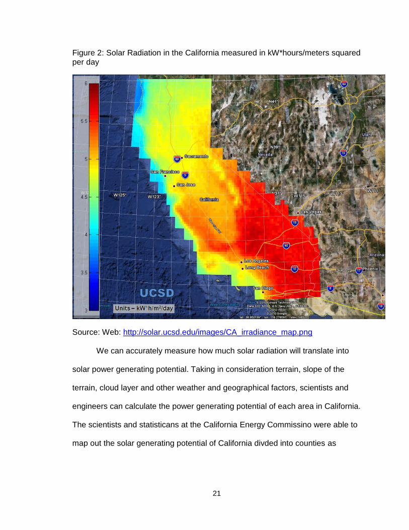
Figure 2: Solar Radiation in the California measured in kW*hours/meters squared per day

Source: Web: http://solar.ucsd.edu/images/CA_irradiance_map.png

We can accurately measure how much solar radiation will translate into

solar power generating potential. Taking in consideration terrain, slope of the

terrain, cloud layer and other weather and geographical factors, scientists and

engineers can calculate the power generating potential of each area in California.

The scientists and statisticans at the California Energy Commissino were able to

map out the solar generating potential of California divded into counties as

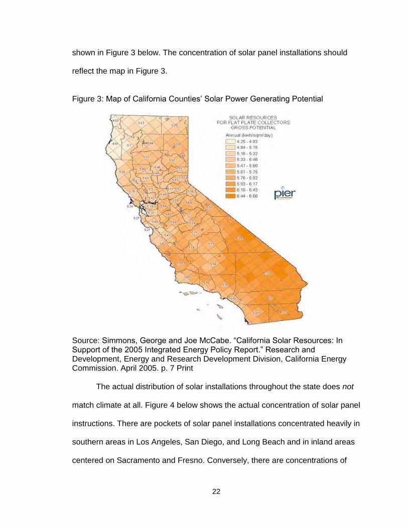
http://solar.ucsd.edu/images/CA_irradiance_map.png

22

shown in Figure 3 below. The concentration of solar panel installations should

reflect the map in Figure 3.

Figure 3: Map of California Counties’ Solar Power Generating Potential

Source: Simmons, George and Joe McCabe. “California Solar Resources: In Support of the 2005 Integrated Energy Policy Report.” Research and Development, Energy and Research Development Division, California Energy Commission. April 2005. p. 7 Print

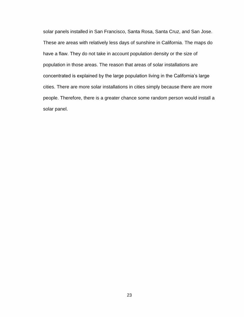
The actual distribution of solar installations throughout the state does not

match climate at all. Figure 4 below shows the actual concentration of solar panel

instructions. There are pockets of solar panel installations concentrated heavily in

southern areas in Los Angeles, San Diego, and Long Beach and in inland areas

centered on Sacramento and Fresno. Conversely, there are concentrations of

23

solar panels installed in San Francisco, Santa Rosa, Santa Cruz, and San Jose.

These are areas with relatively less days of sunshine in California. The maps do

have a flaw. They do not take in account population density or the size of

population in those areas. The reason that areas of solar installations are

concentrated is explained by the large population living in the California’s large

cities. There are more solar installations in cities simply because there are more

people. Therefore, there is a greater chance some random person would install a

solar panel.

24

Figure 4: Heat Map of Solar Installations throughout California Prior to Q3 2011

Source: “Solar Energy Installation Map.” SolarEnergy.net. 2012. Web: http://www.solarenergy.net/Articles/solar-energy-installation-map.aspx

2.2.1 County Level

We can also approach the climate model looking at data on a county level

since my level of analysis is focused on the county level. I use “average days of

one inch or more rainfall” as my dependent variable to predict the percentage of

homes with a solar panel which is placed on the Y axis. I use “average days of

one inch or more rainfall” instead of average days of sunshine in year because

data for average days of sunshine in year for the counties in California was not

readily available. Instead, I opted to use another variable that shares a negative

relationship with the amount of sunshine a county experiences. The average

http://www.solarenergy.net/Articles/solar-energy-installation-map.aspx

25

days of one inch or more rainfall is negatively correlated with the total days of

sunshine. If a county has more average days of one inch rainfall, it is likely to

experience less solar radiation in the same time period. It does not share a

perfect correlation, but it is the best, valid alternative with complete data for all

the counties. Based on the climate model and solar power generating potential,

the relationship between the amount of sunshine and percentage of homes with

a solar panel can be summarized by “The more days of rainfall of one inch or

more a county experiences, the smaller the percentage of homes that will have a

solar panel.”

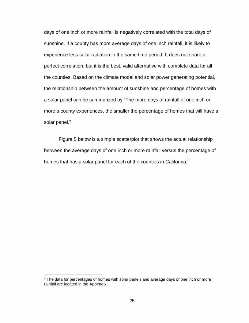
Figure 5 below is a simple scatterplot that shows the actual relationship

between the average days of one inch or more rainfall versus the percentage of

homes that has a solar panel for each of the counties in California.3

3 The data for percentages of homes with solar panels and average days of one inch or more

rainfall are located in the Appendix.

26

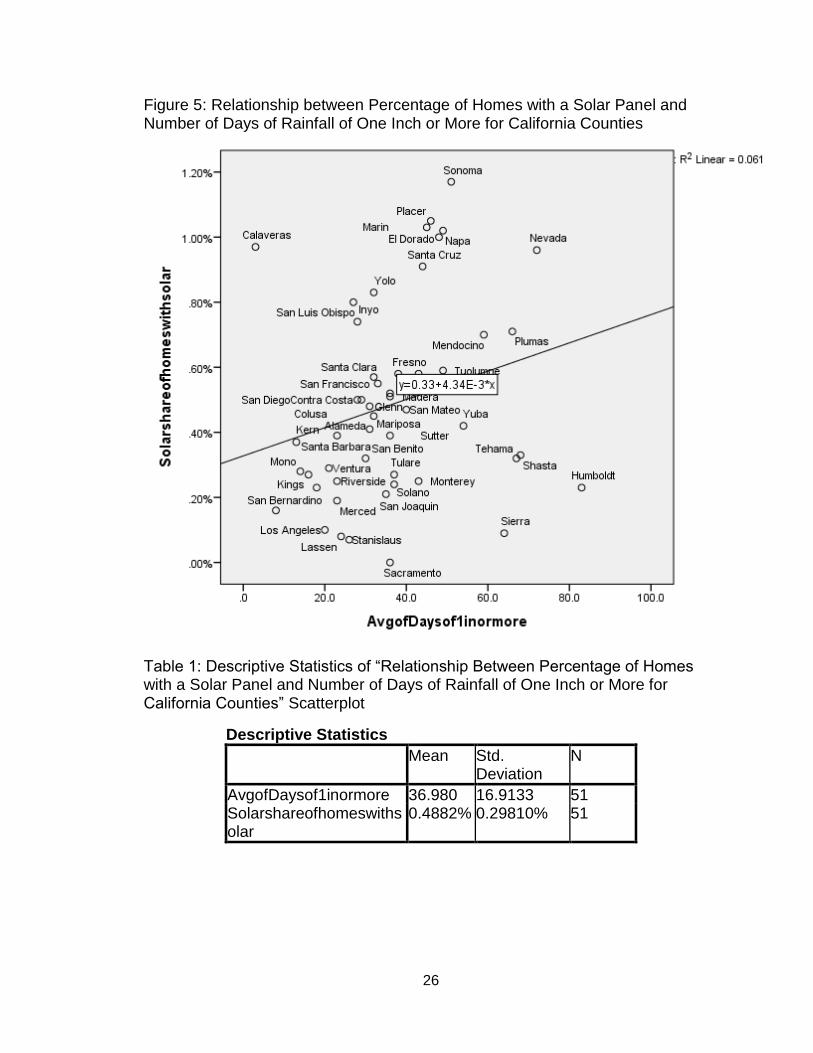
Figure 5: Relationship between Percentage of Homes with a Solar Panel and Number of Days of Rainfall of One Inch or More for California Counties

Table 1: Descriptive Statistics of “Relationship Between Percentage of Homes with a Solar Panel and Number of Days of Rainfall of One Inch or More for California Counties” Scatterplot

Descriptive Statistics

Mean Std. Deviation

N

AvgofDaysof1inormore 36.980 16.9133 51 Solarshareofhomeswithsolar

0.4882% 0.29810% 51

27

The fit line in the scatterplot shows that as the average days of one inch or more

rainfall increases, the greater percentage of the of homes with a solar panel. This

is the opposite of what we expected based on the climate model.4

Let’s look at the some of the cases. Orange County has 18 average

numbers of days per year with rainfall of one inch or more compared to the mean

in the state which is about 37 days of one inch or more rainfall. This is at the

lower end of the spectrum in the state. The expectation would be Orange County

should have a more solar panels per capita than most other counties especially

because it falls outside the standard deviation. However, this is not the case.

Orange County only has 0.23% of its homes with solar panels compared to the

state mean of 0.4882% of homes with a solar panel. Orange County is only 53%

of the California mean of percentage of home with a solar panel. The climate

model fails to predict the outcome in the case of Orange County.

Santa Cruz averages 44 days of rainfall of one inch or more each year.

This is 7 days above the state average. Yet, the county has 0.91% of homes

covered by solar panels. This is 0.61% higher than the state mean. This is over a

100% increase above the state average. This county has more than double the

days of rainfall compared to Orange County but yet it has more four times the

homes covered with residential solar systems than it.

4 I had to reduce the sample size to 51 counties because some counties had missing data on

percentage of homes with a solar panel side.

28

When comparing two like counties, the failure of climate based model

becomes more apparent. Contrast the cases between San Diego County and

San Francisco County. Both are coastal counties. Both are urban counties with

high densities of residents per square mile. San Francisco has 8,714 people per

square mile and San Diego has 710 people per square mile according to the

2005 estimates by the California Public Utilities Commission. Both counties are

way above the state average of 235.68 people per square mile. Both are wealthy

counties. According to the American Communities Survey (ACS) for years 2007-

2011, the household median incomes for San Diego and San Francisco counties

were $63,857 and $72,947 respectively. These two counties’ household median

incomes were above state’s household median income of $61,632. Both counties

rely on similar industries like tourism, high technology industries like

biotechnology and internet companies, and trade.

The difference is in climate. Although San Diego has an average of 29

days of one inch or more rainfall while San Francisco has 33 days, these

numbers do not present the most accurate description. It seems like the two

counties experience the same amount of sunlight. This is not true. First, San

Diego is located 500 miles south of San Francisco. Due to the angle of the tilt of

the Earth’s axis, San Diego receives more solar radiation.

This is why it is necessary to look at the data on amount of the solar

radiation for each county. Appendix A displays all the solar power generating

potential by county. Solar PV potential is more closely correlated with the amount

29

of solar radiation a county receives in a year. Appendix A clearly shows that the

counties with the most energy potential are the counties that are inland and in the

south of the state. The top five counties are San Bernardino, Inyo, Riverside, Los

Angeles, and San Diego in this order. These are desert and semi-arid areas with

many days of sunshine. San Diego has 3,561,569 MWH (megawatt hours) per

day solar PV potential. This far surpasses San Francisco’s potential of 38,977

MWH per day. Despite the vast difference in solar power potential, San

Francisco has a higher percentage of homes with a solar panel. 0.55% of homes

in San Francisco have a solar panel compared to the 0.50% in San Diego.

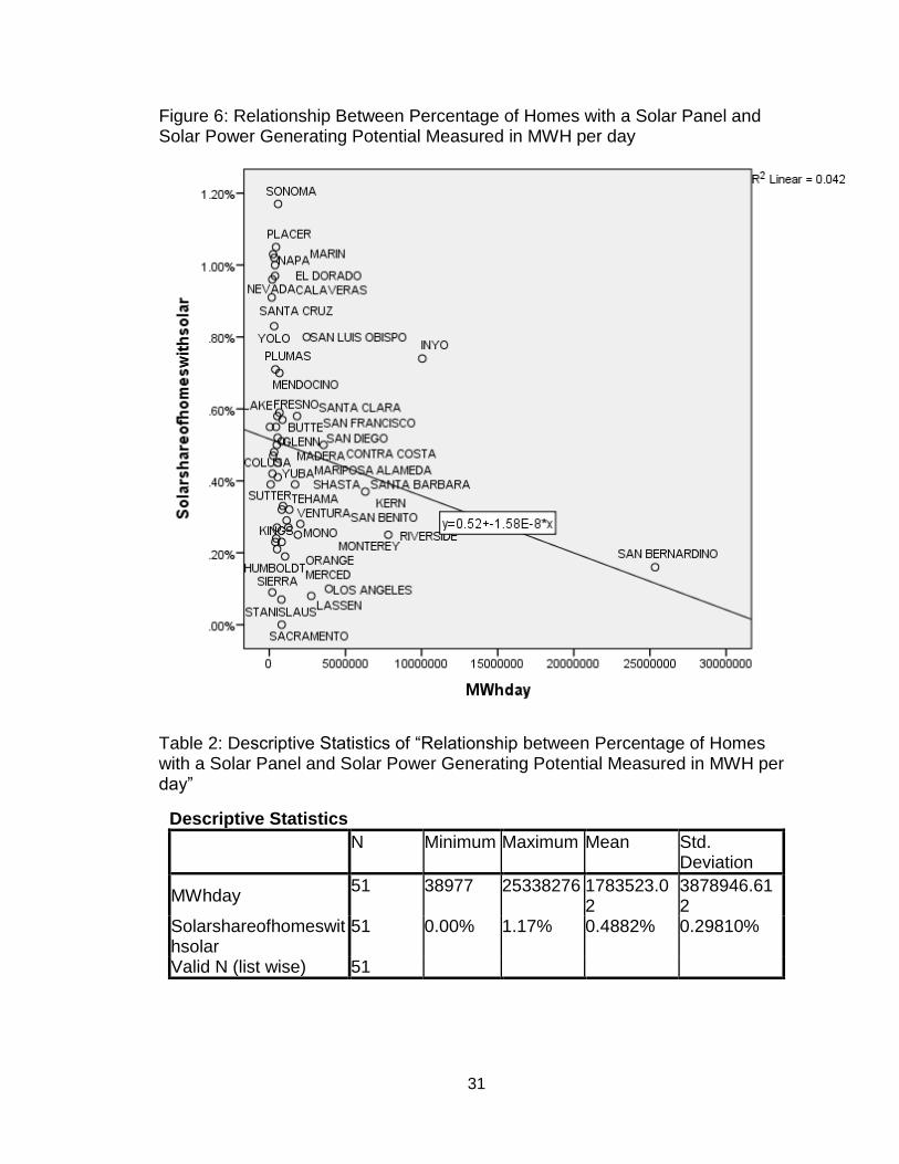
The entire relationship between percentage of homes with a solar panel

and solar power generating potential is displayed in Figure 6 underneath. The fit

line shows as solar power generating potential increases for a county, there will

be a smaller percentage of homes with a solar panel. Figure 6 is consistent with

the previous scatterplot’s statistical relationship. It shows that as the amount of

solar radiation increases, the less likely a Californian will install a solar panel on

their property. This is the opposite of the expectation set by the climate based

model.

The two linear regression’s scatterplots show that climate has little

predictive power in forecasting the percentage of homes with a solar panel in a

California county. The R squares in the Figure 5 is 0.061 and it is 0.042 in Figure

6. Both the relationship between solar radiation and the percentage of homes

30

with a solar panel and the R square values indicate a better variable is needed to

explain the distribution of solar panel installations across the state.

31

Figure 6: Relationship Between Percentage of Homes with a Solar Panel and Solar Power Generating Potential Measured in MWH per day

Table 2: Descriptive Statistics of “Relationship between Percentage of Homes with a Solar Panel and Solar Power Generating Potential Measured in MWH per day”

Descriptive Statistics

N Minimum Maximum Mean Std. Deviation

MWhday 51 38977 25338276 1783523.0

2 3878946.612

Solarshareofhomeswithsolar

51 0.00% 1.17% 0.4882% 0.29810%

Valid N (list wise) 51

32

I theorize that the prevailing political and environmental attitudes in

California counties have an effect on whether or not a person is likely to

purchase and install a solar panel. The main difference between San Diego and

San Francisco counties is political. San Francisco is considered a heavily

Democratic county while San Diego leans Republican. Of the registered voters in

San Francisco, 55% of them are registered Democrats and nine percent were

registered Republicans.5 On the other hand, the Republican Party has a more

prominent presence in San Diego County. Of the registered voters in the general

election of 2008, 35.31% were Democrats compared to 34.07% registered

Republicans. San Diego County has generally voted Republican in presidential

elections. It is only recently that San Diego has voted for the Democratic

candidate for President. Since 1980, San Diego has placed its vote for a

Republican candidate for President six times out of nine. San Francisco is liberal

stronghold and it has not voted for a Republican for President since 1956.6

5 Data obtained from the San Francisco Department of Elections,

http://www.sfelections.org/tools/election_data/. 6 Election data obtained from the California Secretary of State, http://vote.sos.ca.gov/.

33

CHAPTER THREE: THEORITICAL BACKGROUND

In place of climate as a predictive measure for forecasting the likelihood of

a California resident to purchase a solar panel, I will use political and

environmental ideology as the independent variable. I assert that political and

environmental attitudes influence a person’s decision on whether or not a person

purchases and installs a solar panel on their house. The origin of my theoretical

framework is based on Veblen’s idea of conspicuous consumption and consumer

decisions based on political identity. I will take his idea of “dress as an

expression of the pecuniary culture” and transform it into “green products (hybrid

vehicles and solar panels) as an expression of political-environmental culture.” I

will do this by connecting the politics of identity with the politics of consumption.

Finally, I will narrow area of focus to green products specifically solar panels and

elaborate on the “Prius Effect.”

3.1 Veblen’s Concept of Conspicuous Consumption and Identity

Thorstein Veblen at the turn of the 19th century came up with his theory on

social-class consumerism that was arising. The added productivity of the

industrial revolution created the fledging middle class and a class of elite rich

owners of capital. The added surplus income experienced by many gave people

to ability to spend on more goods and a wider range of goods at more frequency.

As class divisions arose between the wealthy, middle class, and the poor, so did

consumer behavior between the income groups. He postulated that the

34

conspicuous consumption by the wealthy was not based on economic

considerations. Why would anyone need more than a few pair of suits or

dresses? The goods that the rich spent lavishly on did produce any immediate

economic benefits. He pointed to goods such as silver flatware and elaborates on

the economic logic behind fashion and dresses for women. The point of the

conspicuous spending is to highlight one’s “pecuniary success” as evidence of

one’s social worth (Veblen 1899). The ability to “consume freely and

uneconomically” is to show others that “he or she is not under the necessity of

earning a livelihood.” (Veblen 1899) He defined the products the rich purchased

as “socially visible” consumer goods which also known as Veblen goods. The

goods are made to be plainly visible to others and send the clear message about

what socio-economic characteristics the buyer possesses.

Veblen’s logic of conspicuous consumption is associated with the notion of

economics and identity. George Akerlof and Rachel Kranton published their

version of the idea in The Quarterly Journal of Economics in August 2000. Like

Veblen, differences in behavior arise from social differences (Akerlof and Kranton

2000, 716). The modeling of identity is based on four precepts (Akerlof and

Kranton 2000, 717):

1. People have identity-based payoffs derived from their own actions.

2. People have identity-based payoffs derived from others’ actions. 3. Third parties can generate persistent changes in these payoffs. 4. Some people may choose their identity, but choice may be

prescribed to others.

35

The most relevant principles in my theoretical framework are points one

and two which I will explain later in the chapter.

On these four tenets, Akerlof and Kranton further expand on the

implications of identity on the field on economics. They identify identity as

“fundamental to behavior, choice of identity may be the most important

‘economic’ decision people make.” (Akerlof and Kranton 2000, 717) They

identify the reason for consumer decisions that run against traditional

economic logic. It is the “bolster a sense of self or to salve a diminished

self-image.” (Akerlof and Kranton 2000, 717) Lastly, consumer behavior

based on identity can create an externality. What this means is “one

person’s actions can have meaning for and evoke responses in others.”

(Akerlof and Kranton, 2000 717)

3.1.1 Applying Veblen Concepts and Identity to Political Science

Now, I need to apply the ideas of Veblen and economic identity to my

study by converting those ideas into political ones. Solar panels are Veblen

goods because when installed on a roof, they are visible to neighbors. Solar

panels instead of communicating class distinction, it meant to signaled to others

that the homeowner is an environmentally conscious person.

As shown in chapter one, solar panels are costlier investments taking at

least several years to break even. Even with incentives provided by the states,

solar panels remain costly. Therefore, I assume that homeowners that decide to

36

purchase solar panels based on non-economic reasons. I assert the reason

behind the people who decide to purchase solar panels do so because they

wanted to bolster their image of an environmentalist.

By installing the solar panels, earlier consumers of solar panels influence

others to purchase solar panels for their homes. This is the externality that is

created. This is logic behind the clustering of solar panels which I will elaborate

on further later on in the chapter.

Although Akerlof and Kranton argue that choice of identity is the most

economic decision, I contend that choice of identity and consumer decisions are

the most important political decisions a person can make. The authors allude to

the importance of political identity. They write, “Politics is often a battle over

identity.” (Akerlof and Kranton 2000, 726). They go on further and say, “Symbolic

acts and transformed identities spur revolutions. The authors cite the French

Revolution changing national subjects into citizens and the Russian Revolution

changing citizens into comrades. The environmental movement that was birthed

in the 1960s made people into environmentally conscious consumers (Shah

2007, 7). I presuppose green consumers are the ones who purchase and install

solar panels in order to display to others in their communities that they are

indeed environmentally conscious consumers.

37

3.2 Identity Politics and Politics of Consumption

How do consumer decisions relate to political identity? Consumer

decisions including the decision to buy a solar panel or not is based on the

“efforts to define and defend who I am.” (Parker 2005, 53) Political activity is

basically is animated by the same logic. And “all politics is identity politics.”

(Parker 2005, 53) “Politics involve making comparisons and choice among- and

commitments to- values and interests and groups and individuals (including

choices not to choose among available choices). The choices and the

commitments we make in politics are ones which we mean to- or by which we

cannot help but- identify ourselves.” (Parker 2005, 53)

The act of buying a solar panel is a political act to define oneself as an

environmentally aware citizen intrinsically, but exhibit that image to others. The

act of buying a solar panel is also meant to differentiate oneself from others in

society. The environmental movement has done a good job at stigmatizing non-

green social behavior. One only has to look at public recycling campaigns that

encourage people to recycle. A person has the choice to recycle or not.

Choosing to recycle does have an associated cost. The act of recycling means

taking the time to learn what and what not to recycle and actually taking the time

and effort to carry out the act. By choosing to recycle especially done in a public

fashion, one can signal to others that they are an environmentalist. The same

logic applies to the purchase of solar panels. However, the decision to purchase

a solar panel carries much more cost than the act of recycling. To do is clear

38

commitment to adhere to sustainable values and a clear indicator of others of the

political-environmental values the purchaser holds.

Recent research done by David Crockett and Melanie Wallendorf and by

Mark Legg, Chun-Hung Tang, and Lisa Slevitch provide empirical evidence that

political ideology affect consumer decision-making. In examining the driving

motivations behind certain destinations tourist choose to vacation at, Legg ET. Al

substituted demographic variables with political ones (Legg 2012, 54). The

scholars found that this was a more “efficient” model. Analyzing the Akaike

Information Criteria (AIC) and Schwartz Criteria (SC) scores of political variables

and demographic variables, models that included “variables that exhibit congruity

between political ideologies of travelers and destinations” improved the predictive

power of destination choice models (Legg 2012, 54). Interestingly, when distance

to destination (considered an additional cost to the tourist) was used as a control

variable, it strengthened the influence political leaning had on the choice of

destination. As costs associated with choices increase, the more powerful the

political variable becomes. This could be true for the decision-making process for

solar panels because of their high costs.

Additionally, Crockett and Wallendorf suggest that consumer choice is

increasingly an important way for citizens to express themselves politically.

People’s “involvement in more traditional acts of political participation is

decreasing.” (Crockett 2004, 525) Traditional acts of political participation include

voting, volunteering for campaigns, and following political events through media.

39

Therefore, the relationship between political-environmental attitudes and the

likelihood to purchase a solar panel should be stronger and increased over the

last ten years.7

3.3 Prius Effect Applied to Solar Panels

Literature from psychology gives insight on whether or not a person’s

values, beliefs, and attitudes impel a person to act a certain way that is

congruous with their system of values. The purpose of psychological research

focuses on the linkage between internal/psychological variables with behavior.

The resulting research “suggests that pro-environmental behavior (PEB)

originates from values, beliefs, and attitudes that orient individuals toward

particular actions.”(Clark 2003, 237) The inquiry determined that attitudes do

influence people to carry out pro-environmental people. This theoretical

framework and empirical evidence from the literature support my main claim that

political-environmental beliefs cause proprietors to buy and install solar panels.

I have mentioned the research conducted by Matthew Kahn in the

introduction. He sought to find out if environmental ideology was a determinant

factor in the purchases of cars. His product of interest was the hybrid vehicle.

Similar to my model, he assumes that a rational environmentalist would take

actions that fit his or her set of sustainable values. He or she would do so even

“willingly sacrifice their scare time and financial resources” to uphold those set of

7 Unfortunately, I do not have year to year data on the number of solar panel installations for each

of the counties. As a consequence, I cannot confirm if the relationship between political-environmental ideology and the propensity to install a solar panel has strengthened over time with a time-series analysis.

40

beliefs (Kahn 2007, 1). We can classify this behavior as “voluntary constraint”.

The first reason for this is to reinforce a certain social image. The particular social

image is hybrid owners are trying to reinforce is the image of a green shopper.

The second reason is to remain credible within a certain political group like the

Green Party. A Green Party member who drives around in a Hummer would be

considered by his or her peers as a non-member since the driver’s decision are

hypocritical (Kahn 2007, 3). Hypocrisy has social consequences. The Hummer

driver could be shunned by other Green Party members.

The effects that Kahn has examined in his report have been classified as

the “Prius Effect” by Steven and Alison Sexton. All the academic literature implies

hybrid car owners particularly Prius owners are motivated by political ideology of

sustainability. They suggest residents with solar panels are motivated by their

environmental politics because of the fact that “solar panel installation and car

ownership decisions are two of the most visible consumption decisions

households make” (Sexton 2011,2). Given the fact that solar panels share many

of the same characteristics as hybrid cars, environmentalists should respond in

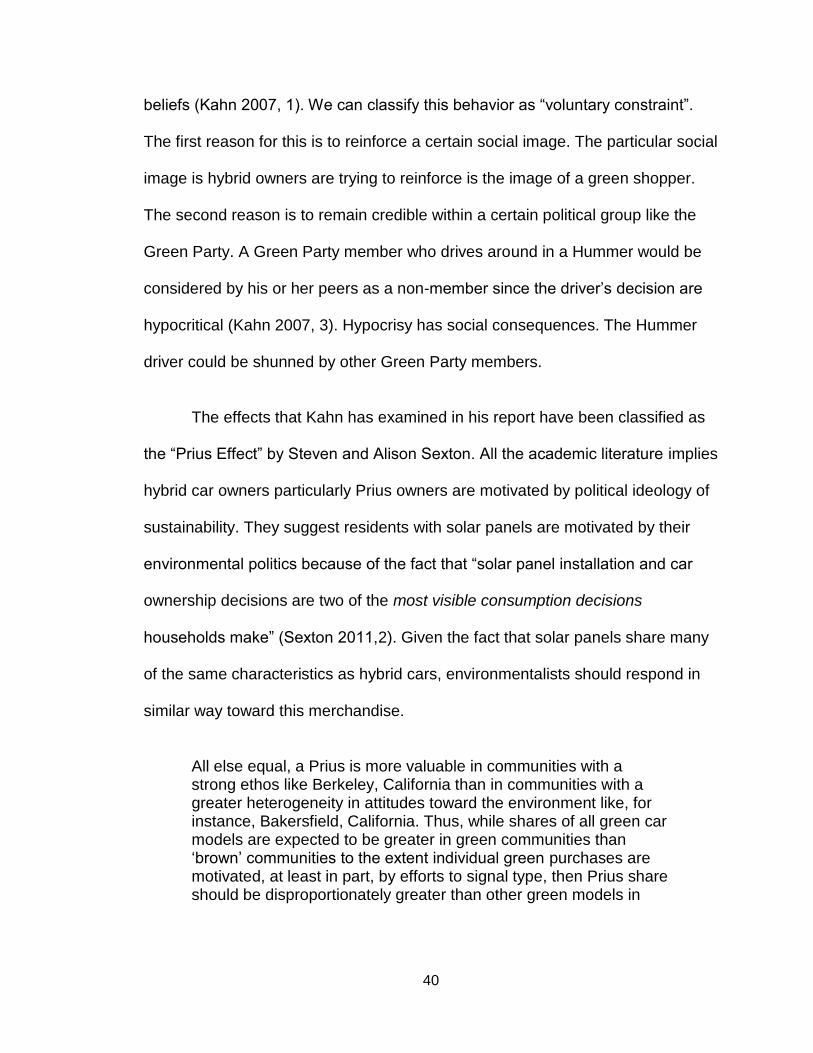
similar way toward this merchandise.

All else equal, a Prius is more valuable in communities with a strong ethos like Berkeley, California than in communities with a greater heterogeneity in attitudes toward the environment like, for instance, Bakersfield, California. Thus, while shares of all green car models are expected to be greater in green communities than ‘brown’ communities to the extent individual green purchases are motivated, at least in part, by efforts to signal type, then Prius share should be disproportionately greater than other green models in

41

these communities because of its unique capacity to signal green type (Sexton 2011, 3)

My model anticipates a similar model of behavior. Solar panels should be

more valued in green communities and less so in brown districts. Thus,

the share of solar panels in a green county should be higher than a brown

county. Using the same line of reasoning, counties that are more

Democratic should have a higher share of solar panels compared to

Republican counties.

3.3.1 Spatial Clustering of Solar Panels

The distribution of Prius locations against the registered Democrats in the

state of Washington organized by zip code is derived from Sexton’s summary

statistics. The geographical distributions of Priuses are represented in Figure 7.

Each green dot represents five Priuses. Darker shades of blue signify that a. zip

code had a greater share of vote that voted for Barack Obama in the 2008

election. The darker the color, the more Democratic the zip code. The large

number of Priuses is concentrated in cities like Seattle and Spokane that are

heavily Democratic. There are very few Priuses in zip codes that had smaller

vote share for Obama in the 2008 election.

42

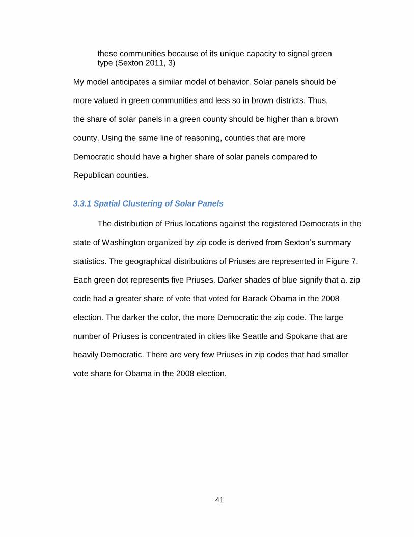
Figure 7: Prius Ownership and Obama Vote Share 2008 Election in Washington (1 dot represents 5 Priuses)

Source: Sexton, Steven and Alison Sexton. “Conspicuous Conservation: The Prius Effect and Willingness to Pay for Environmental Bona Fides.” The Selected Works of Steven E. Sexton. 2011. P. 15. Print.

If the distribution of Prius car owners strongly correlates with the level of

Democratic vote in the zip code, the distribution of solar panels should correlate

strongly with the share of Democratic vote as well. My model predicts counties

that vote more in favor of environmental ballot initiatives, have a greater

percentage of registered Democrats and Greens, and show more commonality

43

with sustainable principles through public opinion surveys should also have more

solar panels per capita.

The distribution of solar panels in the Bay Area affirms my hypothesis. A

study conducted by Bryan Bollinger and Kenneth Gillingham looked at the peer

effects of solar panels. They posited that social interactions propelled neighbors

to buy and install PV panels because the presence of an already existing solar

panel. Bollinger and Gillingham found “an additional installation increases the

probability of an adoption in the zip code by 0.78 percentage points.” (Bollinger

2012, 1) This confirms the occurrence of political-environmental signaling.

What is more interesting is the location of the clusters of solar panels.

Figure 8 reveals the various clusters of PV panels in the Bay Area. There are

four clusters of solar panels located in Marin, San Francisco, Berkeley, and

Santa Clara. These cities and corresponding counties are heavily Democratic

and are densely populated municipalities. The analysis cites “more densely

populated zip codes tend to have more installations, yet there densely populated

zip codes with a few installations, and less densely populated ones with many

installations.” (Bollinger 2012, 10) I explain differences in the uptake of solar

panels in the Bay Are as a result of variances in political beliefs. The authors

mention the differences could be explained by the “clustering of environmental

preferences.” (Bollinger 2012, 11) I would amend “environmental preferences” to

“political-environmental preferences.”

44

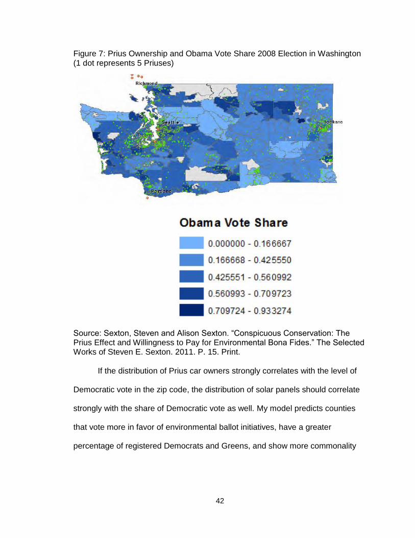
Figure 8: Clustering of Solar PV Panels in the Bay Area

Source: 3Bollinger, Bryan and Kenneth Gillingham. “Peer Effects in the Diffusion of Solar Photovoltaic Panels.” Journal of Marketing Science Volume 31, Number 6. 2012. P.32. Print.

3.4 Theoretical Framework for my Independent Variables

The purpose of this section is the lay out the framework of my model

supported by prior literature. The first study that I drew inspiration from is Kahn

and Matsusaka’s study, Demand for Environmental Goods: Evident from Voting

Patterns on California Initiatives. They use voting behavior of California voters on

16 ballot initiatives on a county level to characterize the demand for

45

environmental goods. Their focus is economic. My focus is on the political side of

the story. I argue that the demand for environmental goods is originates from a

person’s political background. They point the advantage of using ballot initiatives

as the independent variable because there is a cost in voting and the result of the

election also has costs most likely in form of higher taxes. I emulate the

methodology used by Kahn and Matsusaka. In their paper, they merged “county

vote totals on each initiative with demographic and economic variables.” (Kahn

1997, 139) What I did differently is to use demographic and economic variables

as control variables. They found that the wealthy was less likely vote for public

environmental goods because they had to ability purchase the same goods

privately. Solar panels on the other hand are an expensive investment. In order

to purchase a solar panel system, a person’s income must be able to the

thousands of dollars to finance asset.

My inspiration for utilizing the direct survey method comes from another

paper, Internal and External Influences on Pro-environmental Behavior:

Participation in a Green Electricity Program. Clark et al. evaluated the drivers of

pro-environmental behavior. The study analyzed data from a mail survey to

gauge participants and non-participants in a green electricity program. The

survey conducted by Clark et al. asked respondents a series of questions that

ranked their scale of “greenness”. For example, one of the questions asked how

strongly they agreed or disagreed with the statement, “The balance of nature is

delicate and easily upset by human activity.” (Clark 2002, 241) They had to ability

46

to scale their answer from one extreme to another. The surveys that I exploit for

data from the Public Policy Institute of California share many of the same

characteristics. Both are randomized. Both gauge people’s attitudes toward

environmental issues. Both have scaled answers.

My model using party identification is based off the inquiry conducted by

Dora Costa and Matthew Kahn. Their experiment, Energy Conservation

“Nudges” and Environmentalist Ideology: Evidence from a Randomized

Residential Electricity Field Experiment. They show that electricity conservation

nudge in the form of a feedback is responded to differently by liberals and

conservatives. Asking for feedback is shown to help “nudge” residents in

conserving energy, but the strategy backfires on conservatives. Their regression

estimates a household that is Democratic, donates to pro-environmental

pressure groups, and live in a liberal neighborhood will reduce its electricity

usage by three percentage points in response to a nudge (Costa 2010).

Conservatives act in an opposite fashion increasing their consumption by one

percentage point. For my inquiry, I substitute liberal and conservative with

Democrat and Republican. Democrats and Republicans should behave in a

similar fashion toward solar panels.

47

CHAPTER FOUR: RESULTS

Looking at the overall picture of all my regression, I can declare my model

and research design have various flaws. These flaws adversely affected the

validity of my study. As it turns out, many of my regressions were statistically

insignificant. I will further elaborate on the research design flaws in chapter five.

Despite this blemish, my model does draw attention to certain trends in the

regressions.

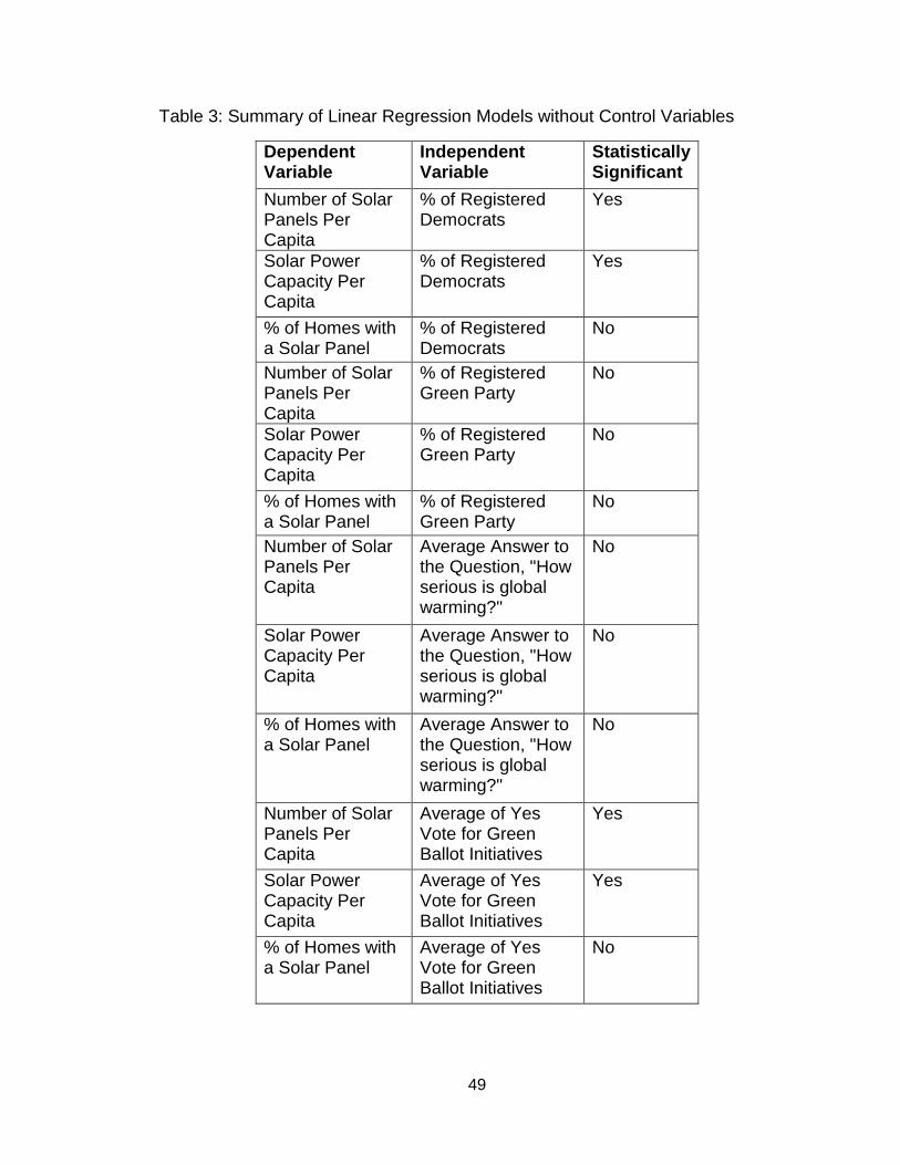
The first half of my regressions did not incorporate a control variable.

Despite this limitation, the statistically significant regressions do give some

insight behind the factors that influence a person’s decision to purchase a solar

panel or not. The results of all the regressions without using control variables are

summarized in Table 3.

I created a checklist of validating if the linear regression was statistically

significant. The steps in my process were to check:

1. The Pearson correlation.

2. The R square value.

3. The Sig. value (significance probability or p-value)

4. The range of values in the 95% confidence interval.

If the Pearson correlation figure is close to zero, the two variables share little or

no correlation with one another. The R squared value measures the proportion of

48

variance in the dependent variable which can be explained by the independent

variable(s). If the R squared value was close to zero, the independent variable

does a poor job explaining the variations in the dependent variable. Finally, I

looked to see if 95% confidence intervals for the coefficients include the value

zero. If it does, then the regression is not statistically significant. Only if a

regression model passes all four steps would I consider the specific regression to

be statistically valid.

There were only four regression analyses that produced statistically

significant results. The four models had number of solar installations per capita

and solar power capacity per capita as the dependent variable. These two

dependent variables almost mirror each other so it is not surprising to see that

both variables to produce a statistically significant result measure against the

percentage of registered Democrats and the share of yes votes for pro-

environmental ballot initiatives. The predictive power of the Democrat variable

even under my flawed model implies that being a Democratic is strongly

correlated with pro-environmental behavior.

49

Table 3: Summary of Linear Regression Models without Control Variables

Dependent Variable

Independent Variable

Statistically Significant

Number of Solar Panels Per Capita

% of Registered Democrats

Yes

Solar Power Capacity Per Capita


Yes

% of Homes with a Solar Panel


No


% of Registered Green Party

No



No



No


Average Answer to the Question, "How serious is global warming?"

No



No



No


Average of Yes Vote for Green Ballot Initiatives

Yes



Yes



No

50

To obtain results for my regressions with control variable, I use

hierarchical multiple regression method. For the first step, I inputted my predictor

variables or control variables. This first step measured the relationship of the

control variables with the dependent variable. The second phase incorporated all

the control variables and my independent variable into the analysis. SPSS

constructed a linear equation with the associated beta values of each of the

control variable and the independent variable. Then I ran the regression to churn

out mathematical data. I use the same checklist I use for my regressions without

the control variables. As a consequence, none of my multiple regressions can be

considered valid results. Table 4 encapsulate every single multiple regression

that incorporated control variables. The letter “S” designates the variable as

statistically significant. The label “IS” means the variable failed to meet all tests of

validity.

51

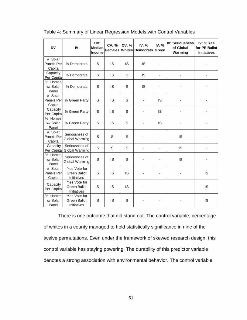
Table 4: Summary of Linear Regression Models with Control Variables

There is one outcome that did stand out. The control variable, percentage

of whites in a county managed to hold statistically significance in nine of the

twelve permutations. Even under the framework of skewed research design, this

control variable has staying powering. The durability of this predictor variable

denotes a strong association with environmental behavior. The control variable,

DV IV

CV:

Median

Income

CV: %

Females

CV: %

Whites

IV: %

Democrats

IV: %

Green

IV: Seriousness

of Global

Warming

IV: % Yes

for PE Ballot

Initiatives

# Solar

Panels Per

Capita

% Democrats IS IS IS IS - - -

Capacity

Per Capita% Democrats IS IS S IS - - -

% Homes

w/ Solar

Panel

% Democrats IS IS S IS - - -

# Solar

Panels Per

Capita

% Green Party IS IS S - IS - -

Capacity

Per Capita% Green Party IS IS S - IS - -

% Homes

w/ Solar

Panel

% Green Party IS IS S - IS - -

# Solar

Panels Per

Capita

Seriousness of

Global WarmingIS S S - - IS -

Capacity

Per Capita

Seriousness of

Global WarmingIS S S - - IS -

% Homes

w/ Solar

Panel

Seriousness of

Global WarmingIS IS S - - IS -

# Solar

Panels Per

Capita

Yes Vote for

Green Ballot

Initiatives

IS IS IS - - - IS

Capacity

Per Capita

Yes Vote for

Green Ballot

Initiatives

IS IS IS - - - IS

% Homes

w/ Solar

Panel

Yes Vote for

Green Ballot

Initiatives

IS IS S - - - IS

52

“percentage of females in a county” remains usable in two permutations.

Perhaps, gender shares a robust relationship with environmental behavior.

The beta value of the coefficients for race matches with my expectations.

The beta value for the standardized coefficient is 0.312. Being a Caucasian

shares a positive relationship with solar PV capacity per capita. Holding all

variables constant, each single unit (1%) increase in the percentage of whites in

a county will predict a .312 Megawatt hour (MWH) per day increase in solar

power generating capacity for a county.

The rest of the chapter will go over every single regression, both using

control variables and not using control variables categorized by the independent

variable. Due to the fact that many of the regressions did not bear usable

outcomes, the focus of the rest of the chapter will be on how I set up the data for

analysis.

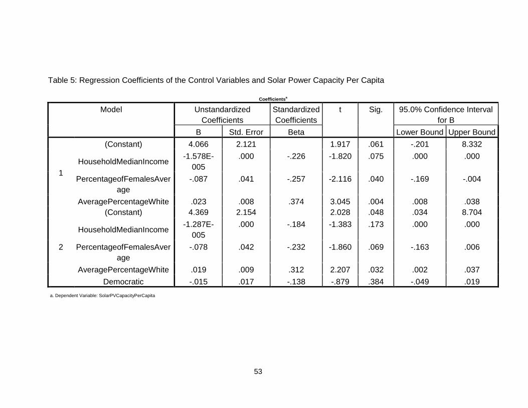
53

Table 5: Regression Coefficients of the Control Variables and Solar Power Capacity Per Capita

Coefficientsa

Model Unstandardized

Coefficients

Standardized

Coefficients

t Sig. 95.0% Confidence Interval

for B

B Std. Error Beta Lower Bound Upper Bound

1

(Constant) 4.066 2.121 1.917 .061 -.201 8.332

HouseholdMedianIncome -1.578E-

005

.000 -.226 -1.820 .075 .000 .000

PercentageofFemalesAver

age

-.087 .041 -.257 -2.116 .040 -.169 -.004

AveragePercentageWhite .023 .008 .374 3.045 .004 .008 .038

2

(Constant) 4.369 2.154 2.028 .048 .034 8.704

HouseholdMedianIncome -1.287E-

005

.000 -.184 -1.383 .173 .000 .000

PercentageofFemalesAver

age

-.078 .042 -.232 -1.860 .069 -.163 .006

AveragePercentageWhite .019 .009 .312 2.207 .032 .002 .037

Democratic -.015 .017 -.138 -.879 .384 -.049 .019

a. Dependent Variable: SolarPVCapacityPerCapita

54

4.1 Party ID

4.1.1 Setting up the Data

First, I averaged the party registration numbers from presidential elections

from 2000-2012. I chose only presidential elections because in between

presidential elections and primary elections have a lower registration rates and

lower voter turnout. This creates a bias of who decides to register to vote for

these elections. The voters that registered to vote in primary elections, special

elections, and in between presidential elections tend to be more extreme both to

the right and left of the political spectrum. I wanted to get a voting population that

is more reflective of the actual population for each of the counties. The resulting

independent variable that was created was the average percentage of

Democrats and Green Party members for each county from 2000-2012.8

4.1.2Results

All the hierarchical multiple regressions using control variables and most

of the linear regressions did not pass the statistical significance tests However,

there two linear regressions that did.

The two linear regressions that passed the test had share of registered

Democrats as the IV. The IV was analyzed against installations per capita and

solar capacity per capita. Figure 9 is the scatterplot highlighting the link between

the IV and installations per capita. The fit line in Figure 9 shows that the number

of installations per capita decreases as the percentage of registered Democrats

8 The average party registration data for Democrats and Greens are displayed in Appendix E.

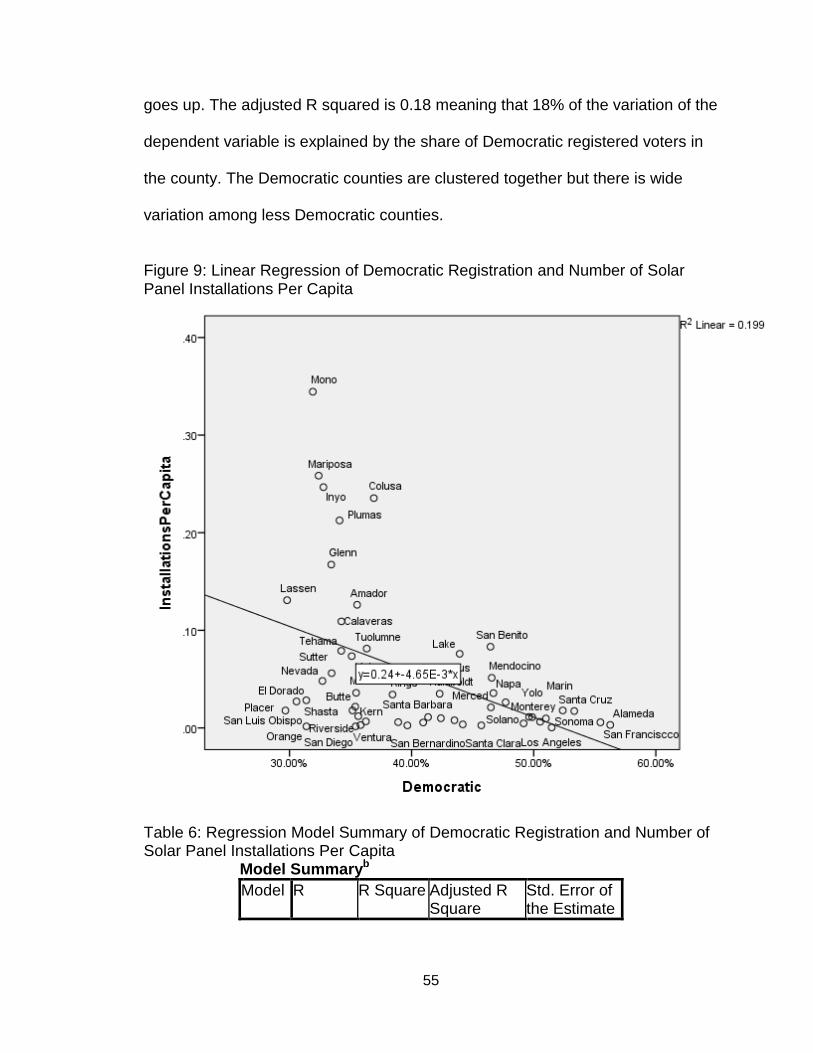
55

goes up. The adjusted R squared is 0.18 meaning that 18% of the variation of the

dependent variable is explained by the share of Democratic registered voters in

the county. The Democratic counties are clustered together but there is wide

variation among less Democratic counties.

Figure 9: Linear Regression of Democratic Registration and Number of Solar Panel Installations Per Capita

Table 6: Regression Model Summary of Democratic Registration and Number of Solar Panel Installations Per Capita

Model Summaryb

Model R R Square Adjusted R Square

Std. Error of the Estimate

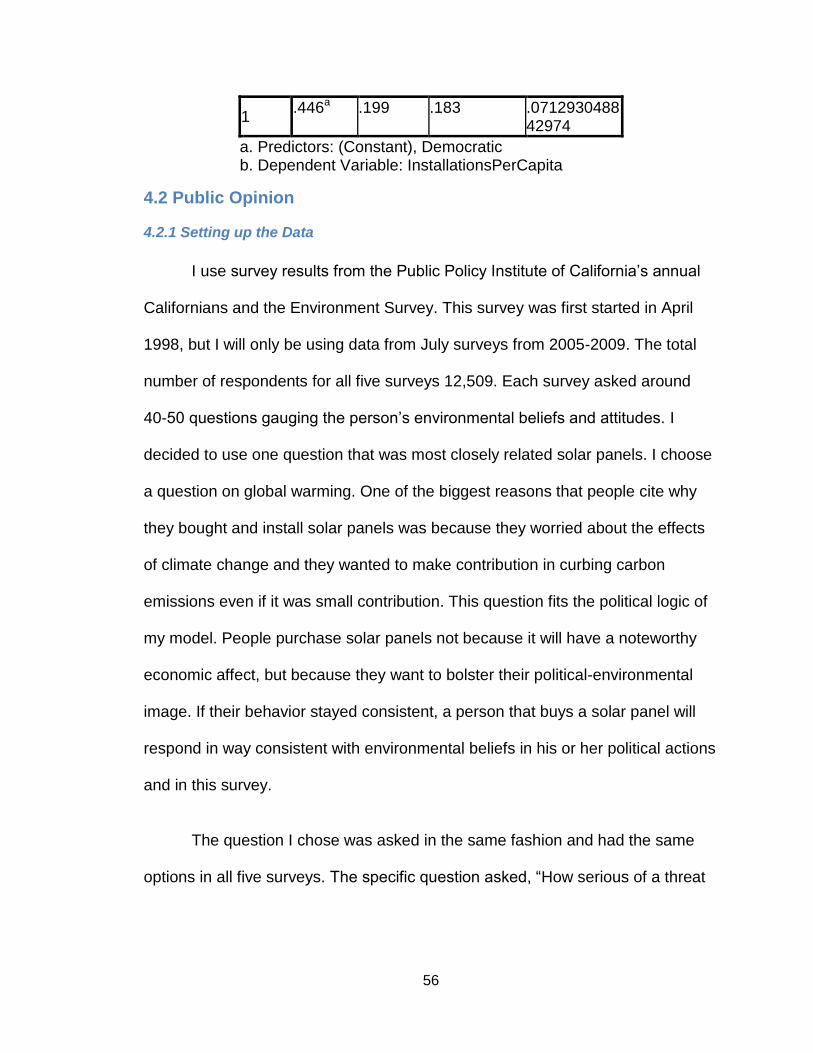
56

1 .446a .199 .183 .0712930488

42974

a. Predictors: (Constant), Democratic b. Dependent Variable: InstallationsPerCapita

4.2 Public Opinion


I use survey results from the Public Policy Institute of California’s annual

Californians and the Environment Survey. This survey was first started in April

1998, but I will only be using data from July surveys from 2005-2009. The total

number of respondents for all five surveys 12,509. Each survey asked around

40-50 questions gauging the person’s environmental beliefs and attitudes. I

decided to use one question that was most closely related solar panels. I choose

a question on global warming. One of the biggest reasons that people cite why

they bought and install solar panels was because they worried about the effects

of climate change and they wanted to make contribution in curbing carbon

emissions even if it was small contribution. This question fits the political logic of

my model. People purchase solar panels not because it will have a noteworthy

economic affect, but because they want to bolster their political-environmental

image. If their behavior stayed consistent, a person that buys a solar panel will

respond in way consistent with environmental beliefs in his or her political actions

and in this survey.

The question I chose was asked in the same fashion and had the same

options in all five surveys. The specific question asked, “How serious of a threat

57

is global warming to the economy and quality of life for California’s future. Do you

think it is:”9

1. Very serious.

2. Somewhat serious.

3. Not too serious.

4. Not serious at all.

5. Don’t know.

6. Refuse to answer.

“Very serious” had a value of one, “somewhat serious” was given a two, “not too

serious” had a three, and “not serious at all” had a value four. Answers five and

six were given assigned numbers of eight and nine respectively. I decided to take

out the respondents that refuse to answer or don’t know. I cannot make any

objective observation if I include them in the analysis. That left me with 12,095

respondents. I decided not to assign weights to answers because that would

arbitrarily skew the results and there is already a tendency for people to answer

the first option because they want to look good in the eyes of the surveyor and

there was no cost in giving an exaggerated answer. In the 2011 survey, 47% of

people interviewed said that global warming was a serious threat compared 11%

that said it was not serious at all (Baldassare 2011, 25). There is evidence of

9 The exact wording of the question was taken from Public Policy Institute of California’s annual

survey, “California and the Environment”. The wording is available in codebook form or in PDF report.

58

some bias here. The average responses to the global question are tabulated in

Appendix F.

The methodology of the survey was sound. The interviews were

conducted over landline phones. Phone numbers was randomly selected by a

computer program. There may have been a slight bias in the survey result in the

later years with the rising prevalence of mobile phones and the decline use of

landlines. In order to avoid biases in age and gender, the researchers in

employed “the last birthday method” for randomly choosing who to interview in

the household. To make sure that immigrants were able to participate in the

study, interviews were conducted in English, Spanish, Chinese (Mandarin and

Cantonese), Vietnamese, and Korean according to the wishes of the interviewee.

This made sure that the assessment was not oversampling native speakers.

4.2.2 Results

All of the regressions, both with control variables and without them, did not

produce statistically significant results.

4.3 Voting Patterns


I use election results from the Office of the Secretary of State of California.

The propositions I included in this study are listed below in Table 6.

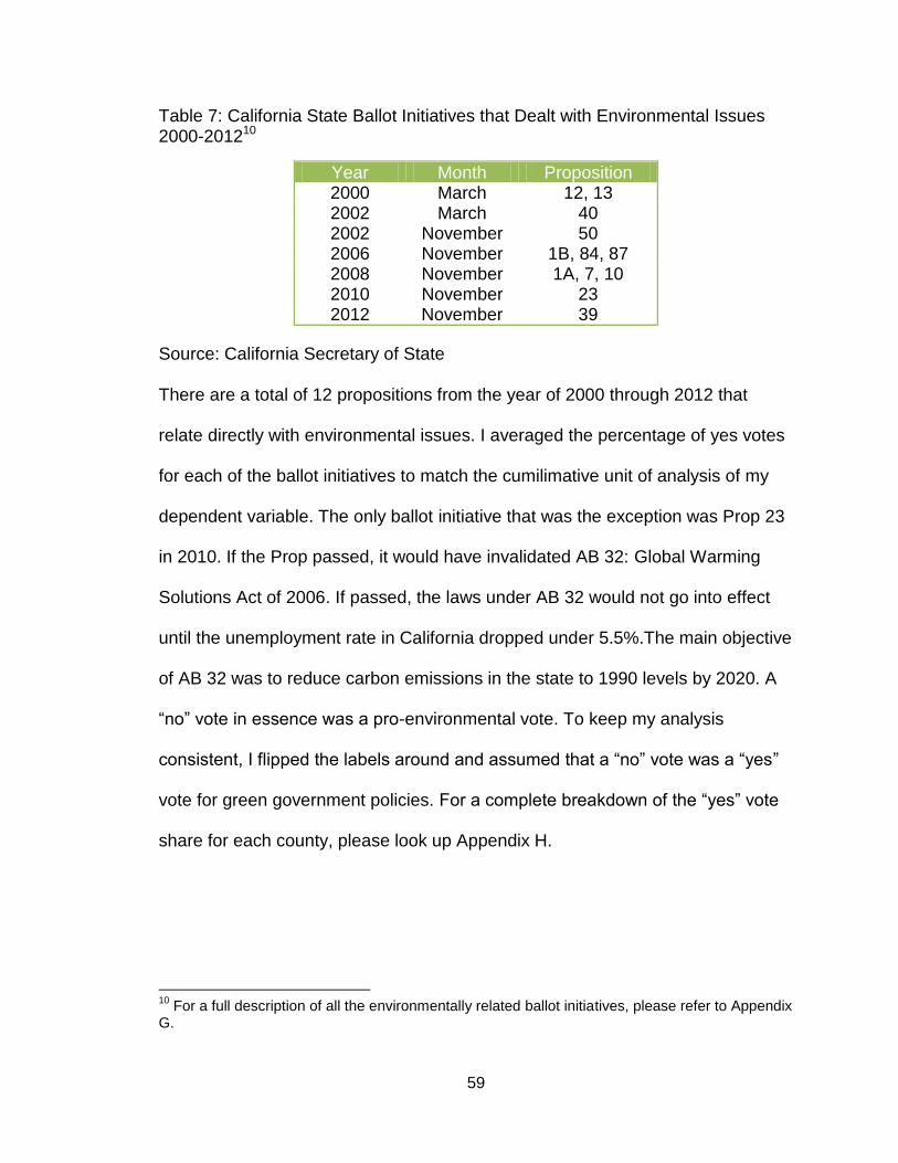
59

Table 7: California State Ballot Initiatives that Dealt with Environmental Issues 2000-201210

Year Month Proposition 2000 March 12, 13 2002 March 40 2002 November 50 2006 November 1B, 84, 87 2008 November 1A, 7, 10 2010 November 23 2012 November 39

Source: California Secretary of State

There are a total of 12 propositions from the year of 2000 through 2012 that

relate directly with environmental issues. I averaged the percentage of yes votes

for each of the ballot initiatives to match the cumilimative unit of analysis of my

dependent variable. The only ballot initiative that was the exception was Prop 23

in 2010. If the Prop passed, it would have invalidated AB 32: Global Warming

Solutions Act of 2006. If passed, the laws under AB 32 would not go into effect

until the unemployment rate in California dropped under 5.5%.The main objective

of AB 32 was to reduce carbon emissions in the state to 1990 levels by 2020. A

“no” vote in essence was a pro-environmental vote. To keep my analysis

consistent, I flipped the labels around and assumed that a “no” vote was a “yes”

vote for green government policies. For a complete breakdown of the “yes” vote

share for each county, please look up Appendix H.

10

For a full description of all the environmentally related ballot initiatives, please refer to Appendix G.

60

4.3.2 Results

There were only two regressions that achieved statistical significance.

They were linear regressions that had solar capacity per capita and installations

per capita. They displayed a similar trend to the regression in Figure 9. If you are

interested in looking up the specific analytics, please refer to the electronic

supplement.

61

CHAPTER FIVE: CONCLUSION

5.1 Findings

The only real takeaway from this study is that percentage of whites in a

county is a good predicator of solar outcome. In the hierarchical multiple

regression, it was statistically significant nine out of twelve times. There is

previous literature indicating that several demographic factors including race

positively influences environmentalism (McMillan, 89). McMillan et al. found

empirical evidence that whites hold more environmental attitudes as measured

by the New Environmental Paradigm (NEP). The authors point to other studies

that show whites are more likely than African-Americans to hold environmental

attitudes (McMillan, 89). Their logic behind this phenomenon was “differences in

socioeconomic status that generally exist between African-Americans and white

cold also provide an explanation for their difference in attitudes.” (McMillan, 91)

In pursuing the research question further, one could take a look at race as a

determining variable. It could be tied with politics since race and politics are not

strange bedfellows.

The surprising thing is that many of the counties inland in and in northwest

California have a high rate of installations per resident. Some of these are more

heavily Republican counties. There are Democratic counties like Marin that have

a high rate of solar outcomes per person, but there are far more Democratic

counties that have low solar outcomes per capita like San Francisco and Santa

62

Clara. I cannot completely reject my three hypotheses because of the flawed

research design, but the data gives weak and inconsistent support for my model.

In many of the cases, the data showed the opposite relationship exists. The data

from my analyses does not support my theory that political-environmental

attitudes are the prime reasons a homeowners decides whether or not to

purchase a solar panel for their property.

5.2 Flaws in my Research Design

There are several flaws that adversely affect the accuracy of my design.

The first one is my unit of analysis. I am analyzing all the different variables on a

county by county basis. The problem is that counties are just too large. San

Bernardino is the largest county in the United States at 20,056.94 square miles

compared the San Francisco which is the smallest county in the California at 47

square miles.11 Population varies widely between counties as well. Los Angeles

is the largest county in the state by population. 9,962,789 call Los Angeles

County their home. On the other side, 1,129 people reside in Alpine County.12

Instead of scaling nominally, I should have scaled all the dependent variables on

a logarithmic scale. This would transform the values according intervals on

magnitude. The use of a logarithmic scale reduces the wide variances of

population between California counties.

11

Numbers are from the US Census. 12

Data also derived from the US Census.

63

Take LA County for example. It has 11,957 solar panel installations. The

population of LA is near 10 million. As a consequence, installations per capita are

small at around 0.0012 installations per Los Angeles resident. Contrast this with

the situation in Yolo County. Yolo is home to 204,118 residents. There are 1,240

solar panel installations in the county. This gives Yolo County 0.0060 solar

panels per resident. Yolo’s number of panel installations per capita is 400% the

rate in Los Angeles. A lot of this may be due to the sheer size of Los Angeles

County which will minimize any effect of political-environmental ideals even they

exist and they actually motivate homeowners to buy and install a solar panel. The

problem lies in my denominator. In my data management, I had to pool all my

control, dependent, and independent variable to the county level. This process

skewed the results.

Two control variables that I did not take into consideration was population

density and whether or not county was predominantly urban, suburban, or rural.

The spatial clustering rationality of solar panels and the maps of the clustering of

solar panels in the Bay Area point to a possible correlation with these two

demographic considerations. However, I could not add more control variables

into my model without running into a degree of freedom problem.

Using counties as my geographical boundaries of analyses meant that my

study would have relied on a low number of samples. This creates a degree of

freedom issue because I cannot incorporate a large number of control variables

into my multiple regression analyses. Instead of using counties as my unit of

64

analysis, it would be better to choose something smaller like ZIP code. That way,

I will get a larger sample size which would increase the accuracy and validity of

my results.

Another flaw of my study is it did not measure changes in political beliefs

across time. Although I had data across time for my independent variables, my

data for my dependent variables were cumulative. In order to match the variables

up, I had average out data on the left handed variables. If I had data over time, I

could measure if political-environmental shifts in beliefs and major events have

an effect on the rate of installations. This is a much stronger way to see if

political-environmental values actually affect consumers compared to my static

model.

5.3 Creating an Ideal Research Design and Research Study

There are two ways to go on from this study. One is to find an alternative

variable to explain the variances in solar panel uptake throughout California. The

question still remains why solar panel installations cluster in certain locations and

there are very few in other like communities.

Another is to revise this study and fix the design flaws. If I had the

opportunity to design the ideal research study to investigate this problem, I would

collect year-year data on California over several years. It would be a time-series

analysis of survey data of new buyers of solar panels. My unit of analysis would

be on the individual level. I would collect a large sampling ranging in the

65

thousands. To collect my data, I would interview the buyers of new solar PV

panels and get their information on their level of education, income, gender,

political party, race, address, opinions of hot environmental issues like climate

change, and other predictors. Then I would ask them was their primary reason in

purchasing a solar system. This is a basic overview of my ideal study. The new

research design fixed the problems in this this thesis.

This puzzle is an important field of study because the growing emphasis

on renewable energy. California passed AB 32 which requires that one-third of

California’s energy come from renewable sources. Electricity generated by

residential solar panels will play a crucial part in meeting that legal requirement.

Government policies and incentives can be made more effective if we can

understand the driving motivation on why people buy green products and how

does the practice spread.

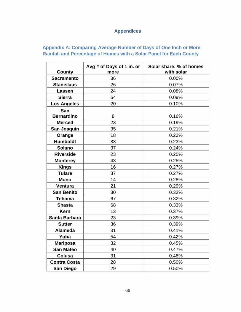
66

Appendices

Appendix A: Comparing Average Number of Days of One Inch or More

Rainfall and Percentage of Homes with a Solar Panel for Each County

County Avg # of Days of 1 in. or

more Solar share: % of homes

with solar

Sacramento 36 0.00%

Stanislaus 26 0.07%

Lassen 24 0.08%

Sierra 64 0.09%

Los Angeles 20 0.10%

San Bernardino 8 0.16%

Merced 23 0.19%

San Joaquin 35 0.21%

Orange 18 0.23%

Humboldt 83 0.23%

Solano 37 0.24%

Riverside 23 0.25%

Monterey 43 0.25%

Kings 16 0.27%

Tulare 37 0.27%

Mono 14 0.28%

Ventura 21 0.29%

San Benito 30 0.32%

Tehama 67 0.32%

Shasta 68 0.33%

Kern 13 0.37%

Santa Barbara 23 0.39%

Sutter 36 0.39%

Alameda 31 0.41%

Yuba 54 0.42%

Mariposa 32 0.45%

San Mateo 40 0.47%

Colusa 31 0.48%

Contra Costa 28 0.50%

San Diego 29 0.50%

http://en.wikipedia.org/wiki/Sacramento_County,_California

http://en.wikipedia.org/wiki/Stanislaus_County,_California

http://en.wikipedia.org/wiki/Lassen_County,_California

http://en.wikipedia.org/wiki/Sierra_County,_California

http://en.wikipedia.org/wiki/Los_Angeles_County,_California

http://en.wikipedia.org/wiki/San_Bernardino_County,_California

http://en.wikipedia.org/wiki/San_Bernardino_County,_California

http://en.wikipedia.org/wiki/Merced_County,_California

http://en.wikipedia.org/wiki/San_Joaquin_County,_California

http://en.wikipedia.org/wiki/Orange_County,_California

http://en.wikipedia.org/wiki/Humboldt_County,_California

http://en.wikipedia.org/wiki/Solano_County,_California

http://en.wikipedia.org/wiki/Riverside_County,_California

http://en.wikipedia.org/wiki/Monterey_County,_California

http://en.wikipedia.org/wiki/Kings_County,_California

http://en.wikipedia.org/wiki/Tulare_County,_California

http://en.wikipedia.org/wiki/Mono_County,_California

http://en.wikipedia.org/wiki/Ventura_County,_California

http://en.wikipedia.org/wiki/San_Benito_County,_California

http://en.wikipedia.org/wiki/Tehama_County,_California

http://en.wikipedia.org/wiki/Shasta_County,_California

http://en.wikipedia.org/wiki/Kern_County,_California

http://en.wikipedia.org/wiki/Santa_Barbara_County,_California

http://en.wikipedia.org/wiki/Sutter_County,_California

http://en.wikipedia.org/wiki/Alameda_County,_California

http://en.wikipedia.org/wiki/Yuba_County,_California

http://en.wikipedia.org/wiki/Mariposa_County,_California

http://en.wikipedia.org/wiki/San_Mateo_County,_California

http://en.wikipedia.org/wiki/Colusa_County,_California

http://en.wikipedia.org/wiki/Contra_Costa_County,_California

http://en.wikipedia.org/wiki/San_Diego_County,_California

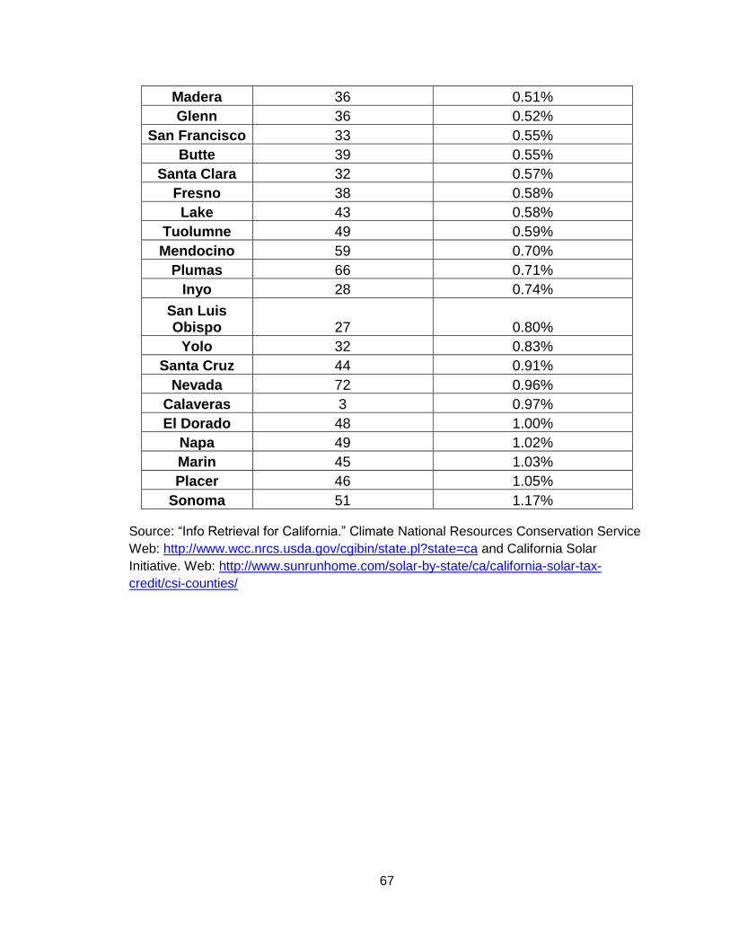
67

Madera 36 0.51%

Glenn 36 0.52%

San Francisco 33 0.55%

Butte 39 0.55%

Santa Clara 32 0.57%

Fresno 38 0.58%

Lake 43 0.58%

Tuolumne 49 0.59%

Mendocino 59 0.70%

Plumas 66 0.71%

Inyo 28 0.74%

San Luis Obispo 27 0.80%

Yolo 32 0.83%

Santa Cruz 44 0.91%

Nevada 72 0.96%

Calaveras 3 0.97%

El Dorado 48 1.00%

Napa 49 1.02%

Marin 45 1.03%

Placer 46 1.05%

Sonoma 51 1.17%

Source: “Info Retrieval for California.” Climate National Resources Conservation Service

Web: http://www.wcc.nrcs.usda.gov/cgibin/state.pl?state=ca and California Solar

Initiative. Web: http://www.sunrunhome.com/solar-by-state/ca/california-solar-tax-

credit/csi-counties/

http://en.wikipedia.org/wiki/Madera_County,_California

http://en.wikipedia.org/wiki/Glenn_County,_California

http://en.wikipedia.org/wiki/San_Francisco_County,_California

http://en.wikipedia.org/wiki/Butte_County,_California

http://en.wikipedia.org/wiki/Santa_Clara_County,_California

http://en.wikipedia.org/wiki/Fresno_County,_California

http://en.wikipedia.org/wiki/Lake_County,_California

http://en.wikipedia.org/wiki/Tuolumne_County,_California

http://en.wikipedia.org/wiki/Mendocino_County,_California

http://en.wikipedia.org/wiki/Plumas_County,_California

http://en.wikipedia.org/wiki/Inyo_County,_California

http://en.wikipedia.org/wiki/San_Luis_Obispo_County,_California

http://en.wikipedia.org/wiki/San_Luis_Obispo_County,_California

http://en.wikipedia.org/wiki/Yolo_County,_California

http://en.wikipedia.org/wiki/Santa_Cruz_County,_California

http://en.wikipedia.org/wiki/Nevada_County,_California

http://en.wikipedia.org/wiki/Calaveras_County,_California

http://en.wikipedia.org/wiki/El_Dorado_County,_California

http://en.wikipedia.org/wiki/Napa_County,_California

http://en.wikipedia.org/wiki/Marin_County,_California

http://en.wikipedia.org/wiki/Placer_County,_California

http://en.wikipedia.org/wiki/Sonoma_County,_California

http://www.wcc.nrcs.usda.gov/cgibin/state.pl?state=ca

http://www.sunrunhome.com/solar-by-state/ca/california-solar-tax-credit/csi-counties/


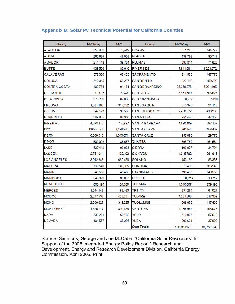
68

Appendix B: Solar PV Technical Potential for California Counties

Source: Simmons, George and Joe McCabe. “California Solar Resources: In Support of the 2005 Integrated Energy Policy Report.” Research and Development, Energy and Research Development Division, California Energy Commission. April 2005. Print.

69

Appendix C: DV, Number of Installations Per Capita and Solar Capacity Per

Capita for California Counties

Row Labels Sum of Number of Solar PV Installations

Sum of Total Solar PV Capacity (kW)

# of Installations Per Capita

Solar PV Capacity Per Capita

Alameda 4427 45727 0.003066339 0.031672578

Amador 152 980 0.126125356 1.302763533

Butte 1044 17909 0.021789527 0.22506657

Calaveras 214 1363 0.109163091 1.127558317

Colusa 56 3351 0.235428632 2.431769836

Contra Costa

4325 33488 0.004665815 0.048193749

El Dorado 1259 6961 0.028323918 0.292561053

Fresno 3836 38378 0.005537855 0.05720115

Glenn 98 632 0.167353419 1.728613012

Humboldt 347 1160 0.034991068 0.361426833

Inyo 86 766 0.246698245 2.548174979

Kern 2128 26307 0.006690899 0.069111079

Kings 404 6282 0.034195626 0.353210619

Lake 379 5284 0.075923099 0.78421856

Lassen 2 6 0.13086792 1.35175003

Los Angeles 11957 123804 0.000465053 0.00480359

Madera 559 6086 0.035960003 0.37143507

Marin 1987 12020 0.017902131 0.184913199

Mariposa 64 243 0.258435493 2.669410391

Mendocino 351 2450 0.051318611 0.530075929

Merced 327 7395 0.021025485 0.217174692

Mono 9 27 0.344433206 3.557690811

Monterey 703 7938 0.011018961 0.11381614

Napa 844 14163 0.035621465 0.367938268

Nevada 915 3871 0.048102311 0.496854389

Orange 5352 41041 0.001555359 0.01606548

Placer 3500 19551 0.017822133 0.184086892

Plumas 23 122 0.212591241 2.195879754

Riverside 4548 42715 0.002864655 0.029589352

Sacramento 2937 36481 0.003618311 0.037373958

San Benito 187 1049 0.083161138 0.858981102

San Bernardino

2731 38609 0.002589746 0.02674979

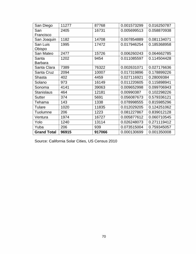
70

San Diego 11277 87768 0.001573299 0.016250787

San Francisco

2405 16731 0.005699513 0.058870938

San Joaquin 1182 14708 0.007854889 0.081134071

San Luis Obispo

1995 17472 0.017946254 0.185368958

San Mateo 2477 15726 0.006260243 0.064662785

Santa Barbara

1202 9454 0.011085597 0.114504428

Santa Clara 7389 76322 0.002631071 0.027176636

Santa Cruz 2094 10007 0.017319896 0.178899226

Shasta 402 4459 0.027116921 0.28009384

Solano 973 16149 0.011220605 0.115898941

Sonoma 4141 39063 0.009652998 0.099706943

Stanislaus 464 12181 0.00990387 0.102298226

Sutter 374 5691 0.056087673 0.579336121

Tehama 143 1338 0.078998555 0.815985296

Tulare 1020 11835 0.012029205 0.124251062

Tuolumne 206 1223 0.081227867 0.839012128

Ventura 1974 16727 0.005877612 0.060710545

Yolo 1240 13114 0.026248073 0.271119412

Yuba 206 939 0.073515004 0.759345057

Grand Total 96915 917066 0.000130699 0.001350008

Source: California Solar Cities, US Census 2010

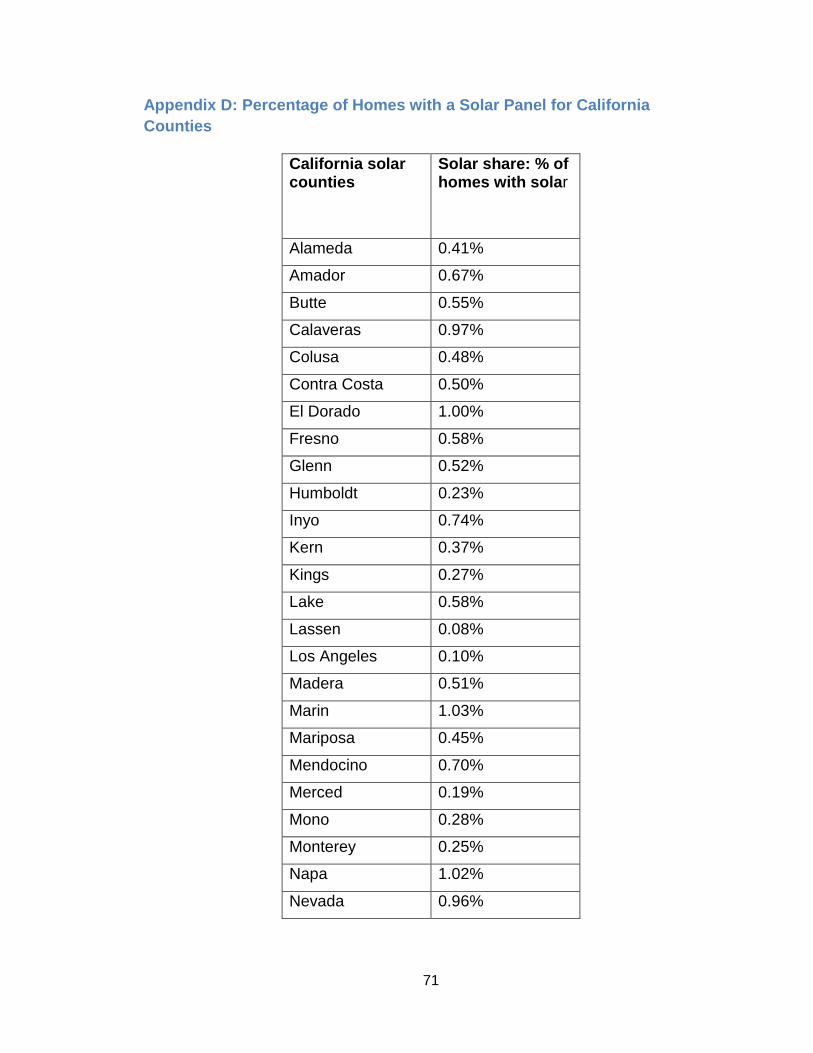
71

Appendix D: Percentage of Homes with a Solar Panel for California

Counties

California solar counties

Solar share: % of homes with solar

Alameda 0.41%

Amador 0.67%

Butte 0.55%

Calaveras 0.97%

Colusa 0.48%

Contra Costa 0.50%

El Dorado 1.00%

Fresno 0.58%

Glenn 0.52%

Humboldt 0.23%

Inyo 0.74%

Kern 0.37%

Kings 0.27%

Lake 0.58%

Lassen 0.08%

Los Angeles 0.10%

Madera 0.51%

Marin 1.03%

Mariposa 0.45%

Mendocino 0.70%

Merced 0.19%

Mono 0.28%

Monterey 0.25%

Napa 1.02%

Nevada 0.96%

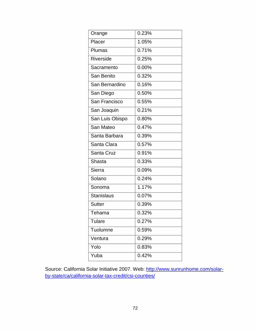
72

Orange 0.23%

Placer 1.05%

Plumas 0.71%

Riverside 0.25%

Sacramento 0.00%

San Benito 0.32%

San Bernardino 0.16%

San Diego 0.50%

San Francisco 0.55%

San Joaquin 0.21%

San Luis Obispo 0.80%

San Mateo 0.47%

Santa Barbara 0.39%

Santa Clara 0.57%

Santa Cruz 0.91%

Shasta 0.33%

Sierra 0.09%

Solano 0.24%

Sonoma 1.17%

Stanislaus 0.07%

Sutter 0.39%

Tehama 0.32%

Tulare 0.27%

Tuolumne 0.59%

Ventura 0.29%

Yolo 0.83%

Yuba 0.42%

Source: California Solar Initiative 2007. Web: http://www.sunrunhome.com/solar-

by-state/ca/california-solar-tax-credit/csi-counties/



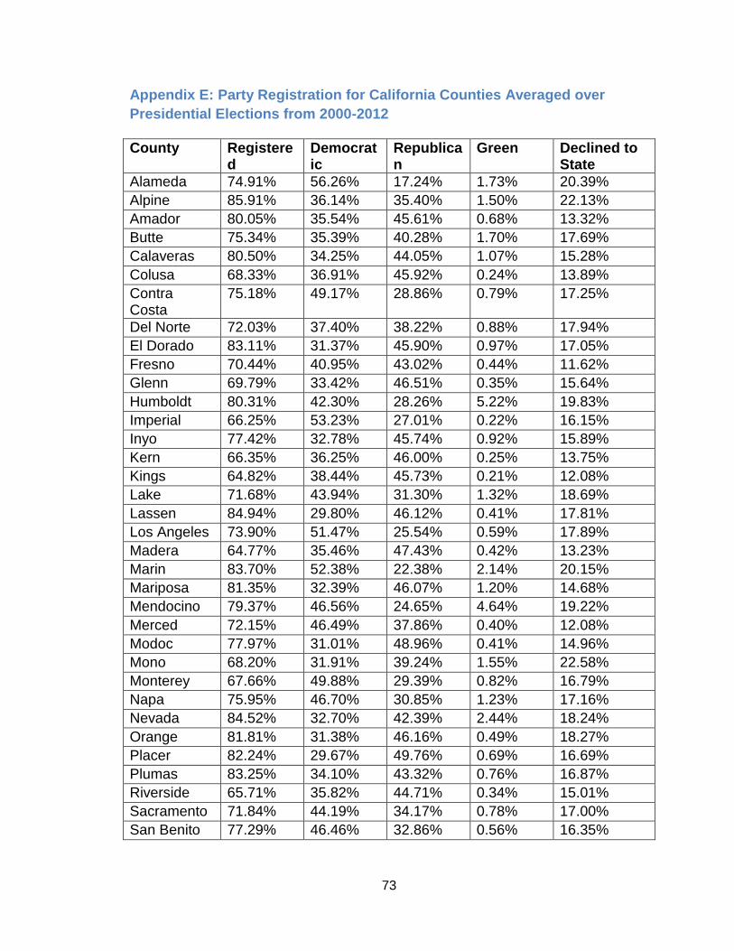
73

Appendix E: Party Registration for California Counties Averaged over

Presidential Elections from 2000-2012

County Registered

Democratic

Republican

Green Declined to State

Alameda 74.91% 56.26% 17.24% 1.73% 20.39%

Alpine 85.91% 36.14% 35.40% 1.50% 22.13%

Amador 80.05% 35.54% 45.61% 0.68% 13.32%

Butte 75.34% 35.39% 40.28% 1.70% 17.69%

Calaveras 80.50% 34.25% 44.05% 1.07% 15.28%

Colusa 68.33% 36.91% 45.92% 0.24% 13.89%

Contra Costa

75.18% 49.17% 28.86% 0.79% 17.25%

Del Norte 72.03% 37.40% 38.22% 0.88% 17.94%

El Dorado 83.11% 31.37% 45.90% 0.97% 17.05%

Fresno 70.44% 40.95% 43.02% 0.44% 11.62%

Glenn 69.79% 33.42% 46.51% 0.35% 15.64%

Humboldt 80.31% 42.30% 28.26% 5.22% 19.83%

Imperial 66.25% 53.23% 27.01% 0.22% 16.15%

Inyo 77.42% 32.78% 45.74% 0.92% 15.89%

Kern 66.35% 36.25% 46.00% 0.25% 13.75%

Kings 64.82% 38.44% 45.73% 0.21% 12.08%

Lake 71.68% 43.94% 31.30% 1.32% 18.69%

Lassen 84.94% 29.80% 46.12% 0.41% 17.81%

Los Angeles 73.90% 51.47% 25.54% 0.59% 17.89%

Madera 64.77% 35.46% 47.43% 0.42% 13.23%

Marin 83.70% 52.38% 22.38% 2.14% 20.15%

Mariposa 81.35% 32.39% 46.07% 1.20% 14.68%

Mendocino 79.37% 46.56% 24.65% 4.64% 19.22%

Merced 72.15% 46.49% 37.86% 0.40% 12.08%

Modoc 77.97% 31.01% 48.96% 0.41% 14.96%

Mono 68.20% 31.91% 39.24% 1.55% 22.58%

Monterey 67.66% 49.88% 29.39% 0.82% 16.79%

Napa 75.95% 46.70% 30.85% 1.23% 17.16%

Nevada 84.52% 32.70% 42.39% 2.44% 18.24%

Orange 81.81% 31.38% 46.16% 0.49% 18.27%

Placer 82.24% 29.67% 49.76% 0.69% 16.69%

Plumas 83.25% 34.10% 43.32% 0.76% 16.87%

Riverside 65.71% 35.82% 44.71% 0.34% 15.01%

Sacramento 71.84% 44.19% 34.17% 0.78% 17.00%

San Benito 77.29% 46.46% 32.86% 0.56% 16.35%

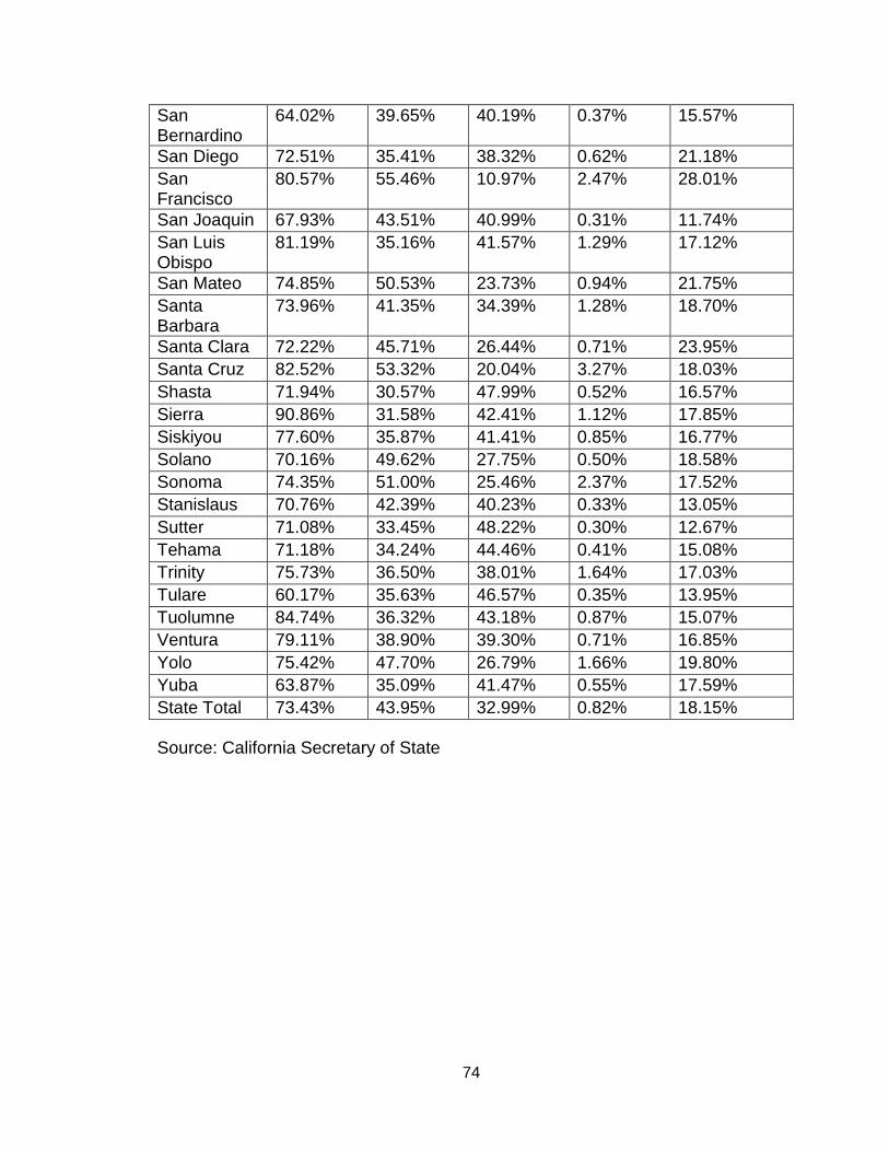
74

San Bernardino

64.02% 39.65% 40.19% 0.37% 15.57%

San Diego 72.51% 35.41% 38.32% 0.62% 21.18%

San Francisco

80.57% 55.46% 10.97% 2.47% 28.01%

San Joaquin 67.93% 43.51% 40.99% 0.31% 11.74%

San Luis Obispo

81.19% 35.16% 41.57% 1.29% 17.12%

San Mateo 74.85% 50.53% 23.73% 0.94% 21.75%

Santa Barbara

73.96% 41.35% 34.39% 1.28% 18.70%

Santa Clara 72.22% 45.71% 26.44% 0.71% 23.95%

Santa Cruz 82.52% 53.32% 20.04% 3.27% 18.03%

Shasta 71.94% 30.57% 47.99% 0.52% 16.57%

Sierra 90.86% 31.58% 42.41% 1.12% 17.85%

Siskiyou 77.60% 35.87% 41.41% 0.85% 16.77%

Solano 70.16% 49.62% 27.75% 0.50% 18.58%

Sonoma 74.35% 51.00% 25.46% 2.37% 17.52%

Stanislaus 70.76% 42.39% 40.23% 0.33% 13.05%

Sutter 71.08% 33.45% 48.22% 0.30% 12.67%

Tehama 71.18% 34.24% 44.46% 0.41% 15.08%

Trinity 75.73% 36.50% 38.01% 1.64% 17.03%

Tulare 60.17% 35.63% 46.57% 0.35% 13.95%

Tuolumne 84.74% 36.32% 43.18% 0.87% 15.07%

Ventura 79.11% 38.90% 39.30% 0.71% 16.85%

Yolo 75.42% 47.70% 26.79% 1.66% 19.80%

Yuba 63.87% 35.09% 41.47% 0.55% 17.59%

State Total 73.43% 43.95% 32.99% 0.82% 18.15%

Source: California Secretary of State

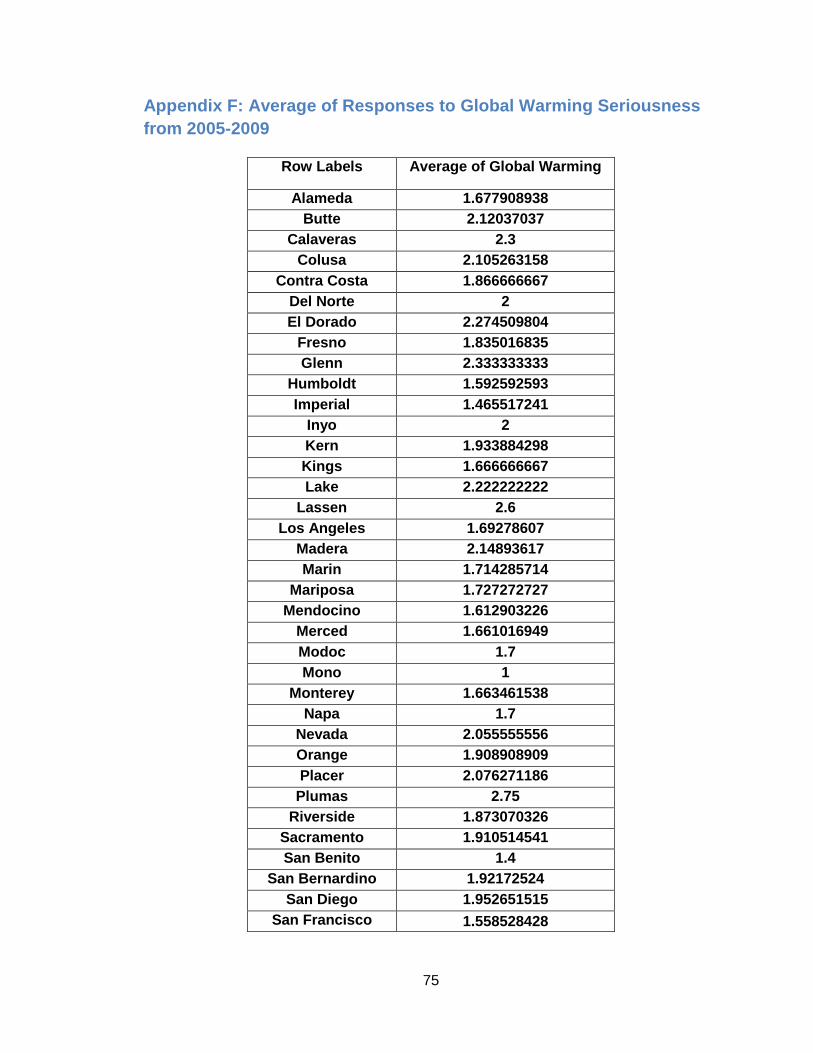
75

Appendix F: Average of Responses to Global Warming Seriousness

from 2005-2009

Row Labels Average of Global Warming

Alameda 1.677908938

Butte 2.12037037

Calaveras 2.3

Colusa 2.105263158

Contra Costa 1.866666667

Del Norte 2

El Dorado 2.274509804

Fresno 1.835016835

Glenn 2.333333333

Humboldt 1.592592593

Imperial 1.465517241

Inyo 2

Kern 1.933884298

Kings 1.666666667

Lake 2.222222222

Lassen 2.6

Los Angeles 1.69278607

Madera 2.14893617

Marin 1.714285714

Mariposa 1.727272727

Mendocino 1.612903226

Merced 1.661016949

Modoc 1.7

Mono 1

Monterey 1.663461538

Napa 1.7

Nevada 2.055555556

Orange 1.908908909

Placer 2.076271186

Plumas 2.75

Riverside 1.873070326

Sacramento 1.910514541

San Benito 1.4

San Bernardino 1.92172524

San Diego 1.952651515

San Francisco 1.558528428

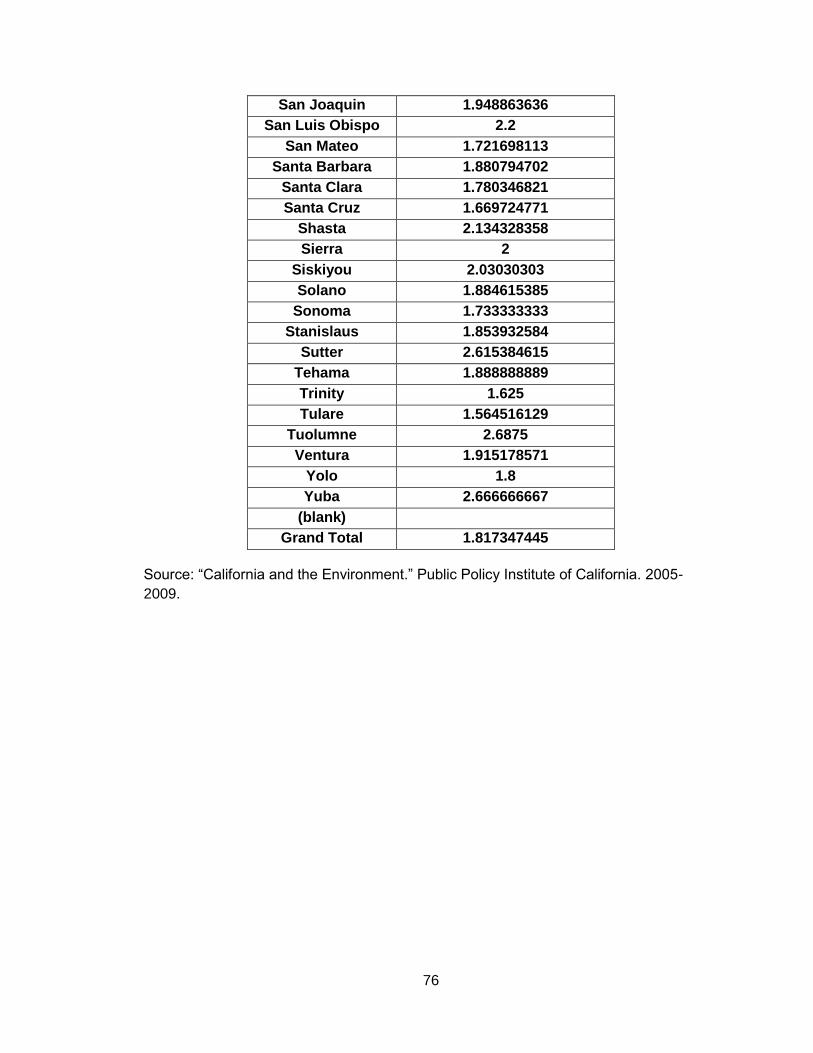
76

San Joaquin 1.948863636

San Luis Obispo 2.2

San Mateo 1.721698113

Santa Barbara 1.880794702

Santa Clara 1.780346821

Santa Cruz 1.669724771

Shasta 2.134328358

Sierra 2

Siskiyou 2.03030303

Solano 1.884615385

Sonoma 1.733333333

Stanislaus 1.853932584

Sutter 2.615384615

Tehama 1.888888889

Trinity 1.625

Tulare 1.564516129

Tuolumne 2.6875

Ventura 1.915178571

Yolo 1.8

Yuba 2.666666667

(blank)

Grand Total 1.817347445

Source: “California and the Environment.” Public Policy Institute of California. 2005-

2009.

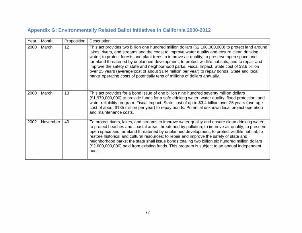
77

Appendix G: Environmentally Related Ballot Initiatives in California 2000-2012

Year Month Proposition Description

2000 March 12 This act provides two billion one hundred million dollars ($2,100,000,000) to protect land around lakes, rivers, and streams and the coast to improve water quality and ensure clean drinking water; to protect forests and plant trees to improve air quality; to preserve open space and farmland threatened by unplanned development; to protect wildlife habitats; and to repair and improve the safety of state and neighborhood parks. Fiscal Impact: State cost of $3.6 billion over 25 years (average cost of about $144 million per year) to repay bonds. State and local parks' operating costs of potentially tens of millions of dollars annually.

2000 March 13 This act provides for a bond issue of one billion nine hundred seventy million dollars ($1,970,000,000) to provide funds for a safe drinking water, water quality, flood protection, and water reliability program. Fiscal Impact: State cost of up to $3.4 billion over 25 years (average cost of about $135 million per year) to repay bonds. Potential unknown local project operation and maintenance costs.

2002 November 40 To protect rivers, lakes, and streams to improve water quality and ensure clean drinking water; to protect beaches and coastal areas threatened by pollution; to improve air quality; to preserve open space and farmland threatened by unplanned development; to protect wildlife habitat; to restore historical and cultural resources; to repair and improve the safety of state and neighborhood parks; the state shall issue bonds totaling two billion six hundred million dollars ($2,600,000,000) paid from existing funds. This program is subject to an annual independent audit.

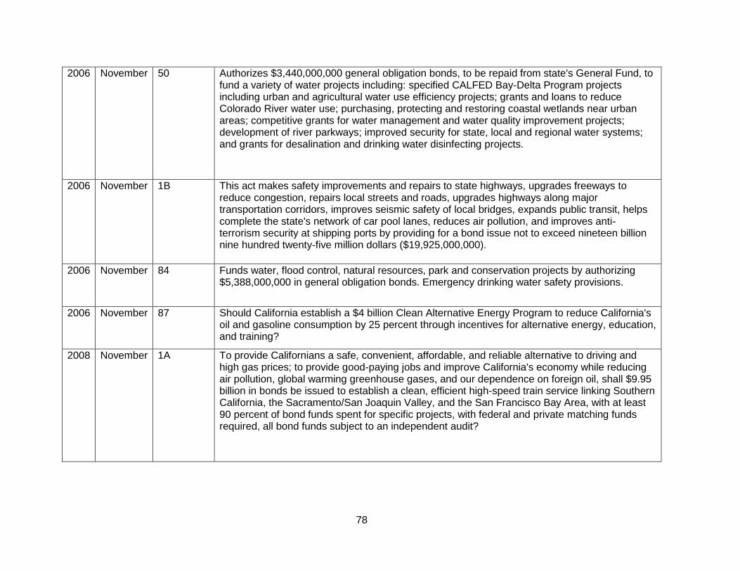
78

2006 November 50 Authorizes $3,440,000,000 general obligation bonds, to be repaid from state's General Fund, to fund a variety of water projects including: specified CALFED Bay-Delta Program projects including urban and agricultural water use efficiency projects; grants and loans to reduce Colorado River water use; purchasing, protecting and restoring coastal wetlands near urban areas; competitive grants for water management and water quality improvement projects; development of river parkways; improved security for state, local and regional water systems; and grants for desalination and drinking water disinfecting projects.

2006 November 1B This act makes safety improvements and repairs to state highways, upgrades freeways to reduce congestion, repairs local streets and roads, upgrades highways along major transportation corridors, improves seismic safety of local bridges, expands public transit, helps complete the state's network of car pool lanes, reduces air pollution, and improves anti-terrorism security at shipping ports by providing for a bond issue not to exceed nineteen billion nine hundred twenty-five million dollars ($19,925,000,000).

2006 November 84 Funds water, flood control, natural resources, park and conservation projects by authorizing $5,388,000,000 in general obligation bonds. Emergency drinking water safety provisions.

2006 November 87 Should California establish a $4 billion Clean Alternative Energy Program to reduce California's oil and gasoline consumption by 25 percent through incentives for alternative energy, education, and training?

2008 November 1A To provide Californians a safe, convenient, affordable, and reliable alternative to driving and high gas prices; to provide good-paying jobs and improve California's economy while reducing air pollution, global warming greenhouse gases, and our dependence on foreign oil, shall $9.95 billion in bonds be issued to establish a clean, efficient high-speed train service linking Southern California, the Sacramento/San Joaquin Valley, and the San Francisco Bay Area, with at least 90 percent of bond funds spent for specific projects, with federal and private matching funds required, all bond funds subject to an independent audit?

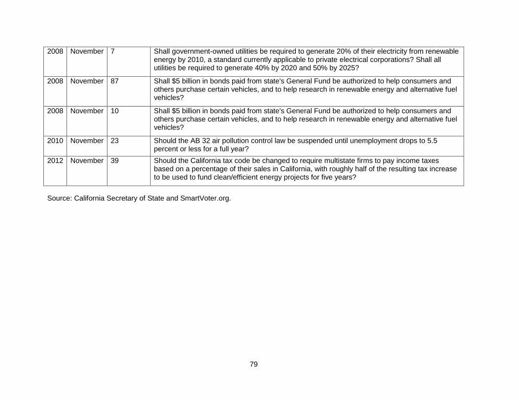
79

2008 November 7 Shall government-owned utilities be required to generate 20% of their electricity from renewable energy by 2010, a standard currently applicable to private electrical corporations? Shall all utilities be required to generate 40% by 2020 and 50% by 2025?

2008 November 87 Shall $5 billion in bonds paid from state's General Fund be authorized to help consumers and others purchase certain vehicles, and to help research in renewable energy and alternative fuel vehicles?

2008 November 10 Shall $5 billion in bonds paid from state's General Fund be authorized to help consumers and others purchase certain vehicles, and to help research in renewable energy and alternative fuel vehicles?

2010 November 23 Should the AB 32 air pollution control law be suspended until unemployment drops to 5.5 percent or less for a full year?

2012 November 39 Should the California tax code be changed to require multistate firms to pay income taxes based on a percentage of their sales in California, with roughly half of the resulting tax increase to be used to fund clean/efficient energy projects for five years?

Source: California Secretary of State and SmartVoter.org.

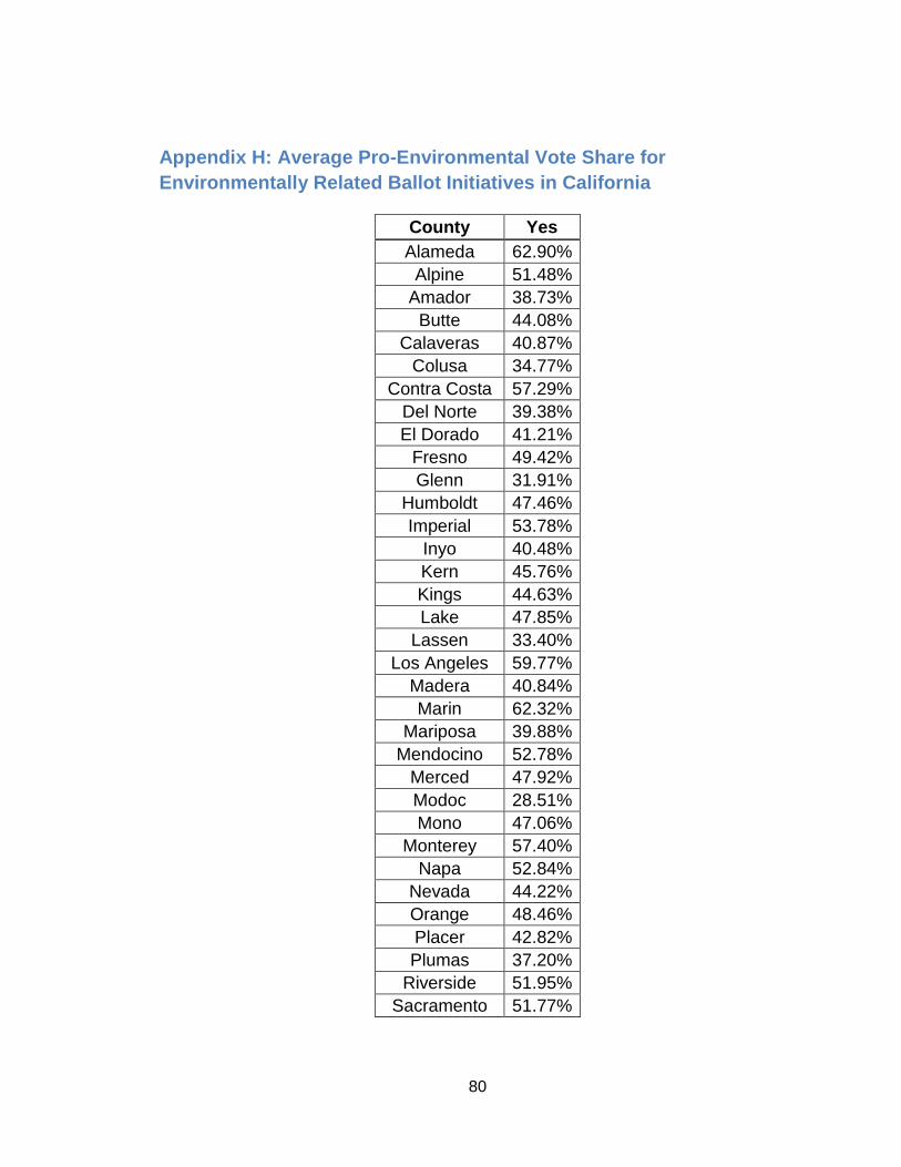
80

Appendix H: Average Pro-Environmental Vote Share for

Environmentally Related Ballot Initiatives in California

County Yes

Alameda 62.90%

Alpine 51.48%

Amador 38.73%

Butte 44.08%

Calaveras 40.87%

Colusa 34.77%

Contra Costa 57.29%

Del Norte 39.38%

El Dorado 41.21%

Fresno 49.42%

Glenn 31.91%

Humboldt 47.46%

Imperial 53.78%

Inyo 40.48%

Kern 45.76%

Kings 44.63%

Lake 47.85%

Lassen 33.40%

Los Angeles 59.77%

Madera 40.84%

Marin 62.32%

Mariposa 39.88%

Mendocino 52.78%

Merced 47.92%

Modoc 28.51%

Mono 47.06%

Monterey 57.40%

Napa 52.84%

Nevada 44.22%

Orange 48.46%

Placer 42.82%

Plumas 37.20%

Riverside 51.95%

Sacramento 51.77%

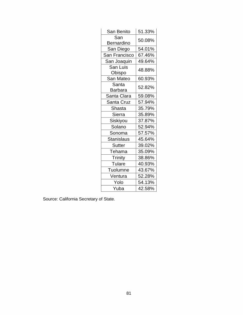
81

San Benito 51.33%

San Bernardino

50.08%

San Diego 54.01%

San Francisco 67.46%

San Joaquin 49.64%

San Luis Obispo

48.88%

San Mateo 60.93%

Santa Barbara

52.82%

Santa Clara 59.08%

Santa Cruz 57.94%

Shasta 35.79%

Sierra 35.89%

Siskiyou 37.87%

Solano 52.94%

Sonoma 57.57%

Stanislaus 45.64%

Sutter 39.02%

Tehama 35.09%

Trinity 38.86%

Tulare 40.93%

Tuolumne 43.67%

Ventura 52.28%

Yolo 54.13%

Yuba 42.58%

Source: California Secretary of State.

82

References

1. Akerlof, George and Rachel Kranton. “Economics and Identity.” Quarterly

Journal of Economics. Volume CXV Issue 3. August 2000. p. 715-753.

Print.

2. Baldassare, Mark, Dean Bonner, Sonja Petek, and Jui Shrestha.

“Californians and the Environment.” PPIC Statewide Survey. Public Policy

Institute of California. July 2011. Print.

3. Bollinger, Bryan and Kenneth Gillingham. “Peer Effects in the Diffusion of

Solar Photovoltaic Panels.” Journal of Marketing Science Volume 31,

Number 6. 2012. P. 900-912. Print.

4. Bradford, Stacey. “Are Hybrid Cars Worth It?” SmartMoney.com. 28

November 2003. Web: http://www.smartmoney.com/spend/family-

money/are-hybrid-cars-worth-it-15101/

5. Chiaro, Del Bernadette. “California’s Solar Cities: Leading the Way to a

Clean Energy Future.” Environment California Research and Policy

Center. Summer 2009. Print.

6. Chiaro, Bernadette and Rachel Gibson. “Government’s Role in Creating a

Vibrant Solar Power Market in California.” Golden Gate University Law

Review. Vol. 36 p. 347-392 (2006). Print

7. Clark, Christopher, Matthew Kotchen, and Michael Moore. “Internal and

External Influences on Pro-environmental Behavior: Participation in a

http://www.smartmoney.com/spend/family-money/are-hybrid-cars-worth-it-15101/

http://www.smartmoney.com/spend/family-money/are-hybrid-cars-worth-it-15101/

83

Green Electricity Program.” Journal of Environmental Psychology. Volume

23. 2003. P. 237-246. Print.

8. Costa, Dora and Matthew Kahn. “Energy Conservation ‘Nudges’ and

Environmentalist Ideology: Evidence from a Randomized Residential

Electricity Field Experiment.” NBER Working Paper. Revised May 2010.

9. Darlin, Damon. “Financially, Solar Power for the Home is a Tough Sell.”

The New York Times, Your Money. 14 April 2007. Web:

http://www.nytimes.com/2007/04/14/business/14money.html

10. Dastrup, Samuel, Joshua Graff Zivin, Dora Costa, and Matthew Kahn.

“Understanding the Solar Home Price Premium: Electricity Generation and

‘Green’ Social Status.” 3 December 2011. Print

11. Davis, Benjamin and Travis Madsen. “California’s Solar Cities 2012:

Leaders in the Race toward a Clean Energy Future.” Environment

California Research and Policy Center. January 2012. Print.

12. Crockett, David and Melanie Wallendorf. “The Role of Normative Political

Ideology in Consumer Behavior.” Journal of Consumer Research. Volume

3, Issue 3. 2004. P. 511-528. Print.

13. Kahn, Matthew and John Matsusaka. “Demand for Environmental Goods:

Evidence from Voting Patterns on California Initiatives.” Journal of Law

and Economics. Volume 40, Number 1. April 1997. P. 137-173. Print.

14. Kahn, Matthew. “Do greens drive Hummers or hybrids? Environmental

ideology as a determinant of consumer choice.” Journal of Environmental

Economics and Management. 13 November 2006. Print.

http://www.nytimes.com/2007/04/14/business/14money.html

84

15. Kahn, Matthew. “Green Market Geography: The Spatial Clustering of

Hybrid Vehicle and LEED Registered Buildings.” The B.E. Journal of

Economic Analysis & Policy. Volume 9 Issue 2. 2009. Print.

16. Kotchen, Matthew and Michael Moore. “Conservation: From Voluntary

Restraint to a Voluntary Price Premium.” Environmental Resource

Economics. (2008). Vol. 40 p. 195-215. Print.

17. Labay, Duncan and Thomas Kinnear. “Exploring the Consumer Decision

Process in the Adoption of Solar Energy Systems.” The Journal of

Consumer Research. Volume 8, Number 3. December 1981. P. 271-278.

Print.

18. Legg, Mark, Chun-Hung Tang, and Lisa Slevitch. “Does Political Ideology

Play a Role in Destination Choice?” American Journal of Tourism

Research. Volume 1, Number 2. 2012. P. 45-58. Print.

19. McMillan, Marybe, Thomas Hoban, William Clifford, and Margaret Brant.

“Social and Demographic Influences on Environmental Attitudes.”

Southern Rural Sociology. Volume 13, Number 1. P. 89-107. Print.

20. Parker, Richard. “Five Theses on Identity Politics.” Harvard Journal of Law

and Public Policy. Volume 29 Issue 1. September 2005. Print.

21. Samuelson, Robert. “Prius Politics.” The Washington Post. 25 July 2007.

Web: http://www.washingtonpost.com/wp-

dyn/content/article/2007/07/24/AR2007072401855.html

http://www.washingtonpost.com/wp-dyn/content/article/2007/07/24/AR2007072401855.html

http://www.washingtonpost.com/wp-dyn/content/article/2007/07/24/AR2007072401855.html

85

22. Sexton, Steven and Alison Sexton. “Conspicuous Conservation: The Prius

Effect and Willingness to Pay for Environmental Bona Fides.” The

Selected Works of Steven E. Sexton. 2011. Print.

23. Shan, Dhvan, Douglas McLeod, Lewis Friedland, and Michelle Nelson.

“The Politics of Consumption/the Consumption of Politics.” Annals of the

American Academy of Political and Social Science. Volume 611. May

2007. P. 6-15. Print.

24. Simmons, George and Joe McCabe. “California Solar Resources: In

Support of the 2005 Integrated Energy Policy Report.” Research and

Development, Energy and Research Development Division, California

Energy Commission. April 2005. Print.

25. Veblen, Thorstein. "The Theory of the Leisure Class: An Economic Study

of Institutions.” Electronic Text Center, University of Virginia Library. Web:

http://xroads.virginia.edu/~hyper/VEBLEN/chap07.html

http://xroads.virginia.edu/~hyper/VEBLEN/chap07.html

Documents

Political Attitudes toward the Environment: The …polisci.ucsd.edu/_files/undergrad/Thesis 2013 Political Attitudes...i Political Attitudes toward the Environment: The Politics of