Embed Size (px)
Citation preview

01 June 2020
POLITECNICO DI TORINORepository ISTITUZIONALE
Vulnerability analysis in an Early Warning System for drought / Angeluccetti, Irene. - (2014).Original
Vulnerability analysis in an Early Warning System for drought
Publisher:
PublishedDOI:10.6092/polito/porto/2543940
Terms of use:openAccess
Publisher copyright
(Article begins on next page)
This article is made available under terms and conditions as specified in the corresponding bibliographic description inthe repository
Availability:This version is available at: 11583/2543940 since:
Politecnico di Torino

POLITECNICO DI TORINO
Doctorate school
PhD in Environment and Territory - Environmental Protection and
Management
XXVI cycle
Final Dissertation
Vulnerability analysis in an Early Warning System for
drought
Angeluccetti Irene
Tutor: Co-tutor:
Prof. Piero Boccardo Ing. Francesca Perez
April 2014

Table of contents
ABSTRACT .................................................................................................................................. 4
ACKNOWLEDGMENTS .............................................................................................................. 5
1 INTRODUCTION ................................................................................................................ 6
2 THE DROUGHT THREAT .................................................................................................... 8
2.1 Drought general concepts and definitions .................................................................. 9
2.1.1 American Meteorological Society definition ....................................................... 9
2.1.2 UNCDD definition .................................................................................................. 9
2.1.3 NDMC definition .................................................................................................... 9
2.2 Hazard, vulnerability and risk general concepts ..................................................... 11
2.2.1 UN/ISDR definitions ............................................................................................. 12
2.2.2 Vulnerability and resilience .................................................................................. 12
2.3 The emergency management ................................................................................. 13
2.4 Early warning systems ............................................................................................. 14
2.5 Drought and food security ...................................................................................... 18
2.6 ITHACA vegetation anomaly monitoring system .................................................. 20
2.6.1 Data input and methodology ............................................................................. 20
2.6.2 Derived products ................................................................................................. 24
3 LITERATURE REVIEW ...................................................................................................... 26
4 DATA AND METHODS ......................................................................................................33
4.1 Data inventory ..........................................................................................................33
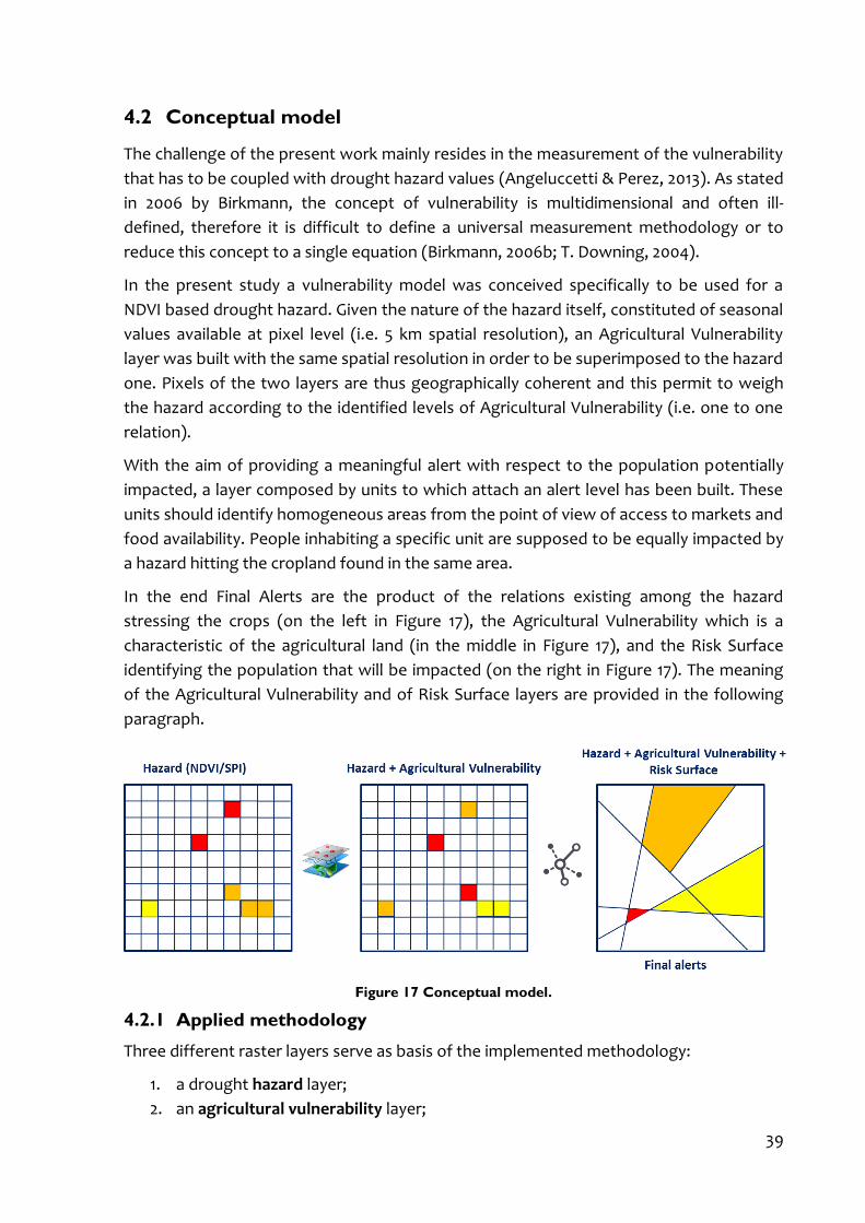
4.2 Conceptual model ................................................................................................... 39
4.2.1 Applied methodology ......................................................................................... 39
4.2.2 Agricultural vulnerability ..................................................................................... 41
4.2.2.1 Soil suitability for crop production - Step 1 ................................................ 42
4.2.2.2 Global Map of Irrigation Areas - Step 2 ...................................................... 44
4.2.2.3 Crop Diversity Index - Step 3 ...................................................................... 45
4.2.3 Risk surface ......................................................................................................... 47
4.2.3.1 Accessibility – Risk surface I ....................................................................... 48
4.2.3.2 Market analysis ........................................................................................... 49
4.2.3.3 Gravity models – Risk surface II .................................................................. 52
4.2.3.4 Gravity models with market flows – Risk surface III ................................. 56
3
4.2.4 Weighted hazard ................................................................................................. 56
4.2.5 Final alert maps .................................................................................................... 57
4.3 Case studies ............................................................................................................. 58
4.3.1 Niger ..................................................................................................................... 58
4.3.1.1 Sahel and Niger Early Warning Systems .................................................... 60
4.3.1.2 Applied model, input and intermediate results .........................................64
4.3.2 Mozambique ........................................................................................................ 76
4.3.2.1 Applied model, input and intermediate results ......................................... 78
4.4 Evaluation phase...................................................................................................... 82
4.4.1 Qualitative evaluation ......................................................................................... 83
4.4.2 Quantitative evaluation ....................................................................................... 85
5 RESULTS .......................................................................................................................... 90
5.1 Qualitative evaluation ............................................................................................ 90
5.2 Quantitative evaluation ......................................................................................... 103
5.3 Discussion .............................................................................................................. 109
CONCLUSIONS AND FURTHER DEVELOPMENTS ................................................................. 113
ANNEXES ................................................................................................................................. 117
Annex I - Matlab script for CDI ........................................................................................... 118
Annex II - CountrySTAT raw data ...................................................................................... 120
Annex III - Developed tools ............................................................................................... 126
BIBLIOGRAPHY ...................................................................................................................... 139

ABSTRACT
Early Warning Systems (EWS) for drought are often based on risk models that do not, or
marginally, take into account the vulnerability factor. The multifaceted nature of drought
(hydrological, meteorological, and agricultural) is source of coexistence for different
ways to measure this phenomenon and its effects. The mentioned issue, together with
the complexity of impacts generated by this hazard, causes the current
underdevelopment of drought EWS compared to other hazards.
In Least Developed Countries, where drought events causes the highest numbers of
affected people, the importance of correct monitoring and forecasting is considered
essential. Existing early warning and monitoring systems for drought, produced at
different geographic levels, provide only in a few cases an actual spatial model that tries
to describe the cause-effect link between where the hazard is detected and where
impacts occur. Integrate vulnerability information in such systems would permit to better
estimate affected zones and livelihoods, improving the effectiveness of produced hazard-
related datasets and maps.
In fact, the need of simplification and, in general, of a direct applicability of scientific
outputs is still a matter of concern for field experts and early warning products end-users.
Even if the surplus of hazard related information produced on the occasion of
catastrophic events has, in some cases, led to the creation of specific data-sharing
platforms, the conveyed meaning and usefulness of each product has not yet been
addressed. The present work is an attempt to fill this gap which is still an open issue for
the scientific community as well as for the humanitarian aid world.
The present study aims at conceiving a simplified vulnerability model to embed into an
existing EWS for drought, which is based on the monitoring of vegetation phenological
parameters, produced using free satellite derived datasets. The proposed vulnerability
model includes (i) a pure agricultural vulnerability and (ii) a systemic vulnerability. The
first considers the agricultural potential of terrains, the diversity of cultivated crops and
the percentage of irrigated area as main driving factors. The second vulnerability aspect
consists of geographic units that model the strategy and possibilities of people to access
marketplaces; these units are shaped on the basis of the physical accessibility of market
locations in one case, and according to a spatial gravity model of market catchments in
other two proposed cases. Results of the model applied to two national case studies and
evaluated with food insecurity data are presented.

5
ACKNOWLEDGMENTS
I firstly thank my supervisor, Professor Boccardo, for its support and for the scientific
advices he provided.
I wish to thank all WFP Niger local office staff, and in particular the VAM unit in the
persons of Lawan Tahirou and Salifou Sanda Ousmane, for their essential and constant
support during my stay in Niger and for sharing their work and knowledge. I thank the
SIMA-Niger for having let me access to their market database. I acknowledge VAM-WFP
headquarter in Rome for providing market locations data and for sharing ideas on food
security monitoring.
I’m grateful to all my ITHACA colleagues for their backing and for making our workplace a
truly pleasant, even if noisy, place. A special thanks goes to Francesca and Alessandro
who strongly contributed to the realization of this work.
I eventually thank my family, none of them knows what I have exactly been doing, but it
was kind of them trying to ask about progress on every Sunday luncheon.
I do thank persons that have been beside me, for having remembered me that it was
worth.
1 INTRODUCTION
Relatively recently, the attention of emergency operators in the context of natural
disasters has been shifted from response and relief to prevention and preparedness
(UN/ISDR, 2004a). Understanding and measuring risk and vulnerability is key to disaster
reduction strategies that in turn have boosted, in the last decades, the development and
use of early warning and monitoring systems (UNEP, 2012).
On the one hand the need of simplification and, in general, of a direct applicability of
scientific outputs is still a matter of concern for field experts and end-users of early
warning products (Bailey, 2013; W Pozzi et al., 2013), though success cases can be
encountered (Hillbruner & Moloney, 2012; Tschirley et al., 2004). On the other hand even
if the surplus of early warning and monitoring information produced on the occasion of
catastrophic events has, in previous cases 0F
1, led to the creation of data-sharing platform 1F
2,
the conveyed meaning and usefulness of each product has not been systematically
addressed nor analyzed to date.
Most of the existent global risk models are not disaster specific, especially for the case of
slow-onset disasters such as drought events. Moreover, the sources and the
implemented processing of data constituting those systems are often not disclosed, thus
compromising their conscious and discriminating use by end-users. Despite the existence
of a consistent number of early warning and monitoring systems for drought produced by
a variety of actors, few cases provide an actual spatial model that tries to represent the
cause-effect linkage between where the hazard is detected and where impacts occur. The
present work is an attempt to fill this gap which is still an open issue for the scientific
community as well as for the humanitarian aid world.
The scientific community has a central and critical role in providing specialized input to
assist governments and communities in developing effective early warning systems.
Scientific expertise is fundamental for risk management support in a variety of ways: i.e.
analyzing natural hazard risks facing communities, designing of scientific and systematic
monitoring and warning services, allowing data exchange and eventually translating
scientific or technical information into comprehensible messages in order to disseminate
understandable warnings to those at risk (UN, 2006).
Until now risk assessment has been predominantly concerned with hazards, for which
there are relatively good data resources and considerable progress have been made.
However after having understood how adverse weather affects food crops and pasture
(i.e. the hazard term of a drought risk equation), the next step is to define and map the
interactions between hazards and people vulnerable to food insecurity (Bohle, Downing,
& Michael, 1994; Eriyagama, Smakhtin, & Gamage, 2010; Wilcox, Kassam, Syroka, &
1 http://horn.rcmrd.org/ 2 http://data.worldbank.org/data-catalog/open-data-for-the-horn
7
Cousins, n.d.). Unfortunately progress made towards the identification and measurement
of social, economic and environmental factors that increase vulnerability are inadequate.
As a result social science data can be difficult to obtain and even when these data are
available they remain underutilized for various reasons (UN, 2006). World summits for
disaster reduction and resilience building, held in the last decade, have stressed the
importance of developing systems of indicators that measure risk of and vulnerability to
disasters both at national and subnational level; the use of recognized indicators would
help decision-makers to estimate the impact of disasters on the societal, economic and
environmental spheres and to disseminate the warnings (UN/ISDR, 2005). Risk experts
have previously stated (Birkmann, 2006a; UN/ISDR, 2004b) that the efforts to develop
new methodologies for measuring risk and vulnerability, and to spread the knowledge of
the existent ones, are to be made by the international community though the
responsibility for the application of disaster and vulnerability reduction strategies belongs
to individual countries. In particular when one considers drought, risk analysis should
address the fact that indirect losses is symptomatic of the paramount role of vulnerability
as a contributing factor to determine these losses (UNDP, 2004); the mediating role of
the economy and society in determining drought-related impacts have become
undeniable (Sen, 1981). Previous studies (Below, Grover-Kopec, & Dilley, 2007) that dealt
with assessing hazard impacts have raised the attention on the fact that, especially for
drought, a few features determine the complexity of risk measurement: the presence of
vulnerable societal assets, the indirect nature of losses, the crucial role of vulnerability in
determining those losses and the difficult nature of drought hazard itself.
The present research tries to address the above-mentioned issues by designing and
implementing a simplified vulnerability model to embed into the ITHACA vegetation
anomaly monitoring system. One of the ambitious goal of this work is thus to translate
the meaning of the purely environmental hazards (based on the analysis of NDVI seasonal
anomalies) into ready-to-use food security alerts. The final alert maps should convey easy
and unmistakable concepts. The driving idea is to use a set of vulnerability indicators,
both environmental and socio-economic, in order to weight the hazard alerts in a way to
improve the readiness of the map already produced and to attach further meaning
related to food insecurity potential.
The present document is structured as follows: a context for drought risk analysis, along
with an overview of possible impacts and the description of the early warning system
targeted by the present research, is provided in Chapter 2; a literature review of existing
models for vulnerability integration in drought monitoring systems is exposed in Chapter
3; data and methodology used for the creation of the simplified vulnerability model is
provided in Chapter 4, together with the model application to two case studies; in
Chapter 5 the outputs, obtained by having applied the model to the case studies, are
compared to evaluation data, both qualitative and quantitative, and the results are
discussed; the last section (CONCLUSIONS AND FURTHER DEVELOPMENTS) is committed
to final conclusions and general evaluation of the research.
2 THE DROUGHT THREAT
This chapter sets the general context of drought as hazard in which the simplified
vulnerability model, final aim of the research, was developed. Most accepted definition
will be given for drought itself, for risk and vulnerability. The ITHACA vegetation anomaly
monitoring system will be also briefly exposed, as well as the drought impacts which the
model aims at detecting and representing (i.e. the food security).
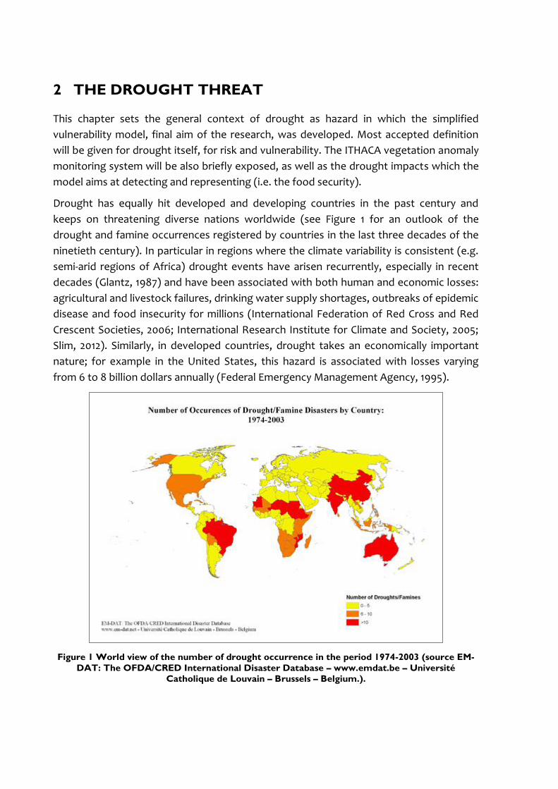
Drought has equally hit developed and developing countries in the past century and
keeps on threatening diverse nations worldwide (see Figure 1 for an outlook of the
drought and famine occurrences registered by countries in the last three decades of the
ninetieth century). In particular in regions where the climate variability is consistent (e.g.
semi-arid regions of Africa) drought events have arisen recurrently, especially in recent
decades (Glantz, 1987) and have been associated with both human and economic losses:
agricultural and livestock failures, drinking water supply shortages, outbreaks of epidemic
disease and food insecurity for millions (International Federation of Red Cross and Red
Crescent Societies, 2006; International Research Institute for Climate and Society, 2005;
Slim, 2012). Similarly, in developed countries, drought takes an economically important
nature; for example in the United States, this hazard is associated with losses varying
from 6 to 8 billion dollars annually (Federal Emergency Management Agency, 1995).
Figure 1 World view of the number of drought occurrence in the period 1974-2003 (source EM-
DAT: The OFDA/CRED International Disaster Database – www.emdat.be – Université
Catholique de Louvain – Brussels – Belgium.).

9
2.1 Drought general concepts and definitions
As early as in 1967 Yevjevich stated that widely diverse views of drought definitions are
one of the principal obstacles to investigations of droughts. The issue of drought
definition is longstanding and has definitely not been resolved until now (Redmond,
2002). That is drought definitions are numerous and vary depending on the variable used
to describe the drought, which is a complex phenomenon that can be defined from
several perspectives (Wilhite & Glantz, 1985). However a widely accepted way to define
drought is through the estimation of its three components: duration, magnitude and
severity (Below et al., 2007; Dracup, Lee, & Paulson, 1980).
A list of most used drought definitions and statements is provided in the following. The
paragraph will offer a broad context in which to set the present study.
2.1.1 American Meteorological Society definition
The Glossary of the American Meteorological Society 2F
3 defines:
Drought as “a period of abnormally dry weather sufficiently long enough to cause
a serious hydrological imbalance.”
Agricultural drought as “conditions that result in adverse crop responses, usually
because plants cannot meet potential transpiration as a result of high atmospheric
demand and/or limited soil moisture.”
Hydrological drought as “prolonged period of below-normal precipitation,
causing deficiencies in water supply, as measured by below-normal streamflow,
lake and reservoir levels, groundwater levels, and depleted soil moisture.”
Socio-economic drought: where the effects of the previous three conditions begin
to affect human economic activity and cause problems for people living in
affected regions.
2.1.2 UNCDD definition
Article 1 of the United Nations Convention to Combat Desertification (UNCCD)3 F
4 defines
drought as “the naturally occurring phenomenon that exists when precipitation has been
significantly below normal recorded levels, causing serious hydrological imbalances that
adversely affect land resource production systems”.
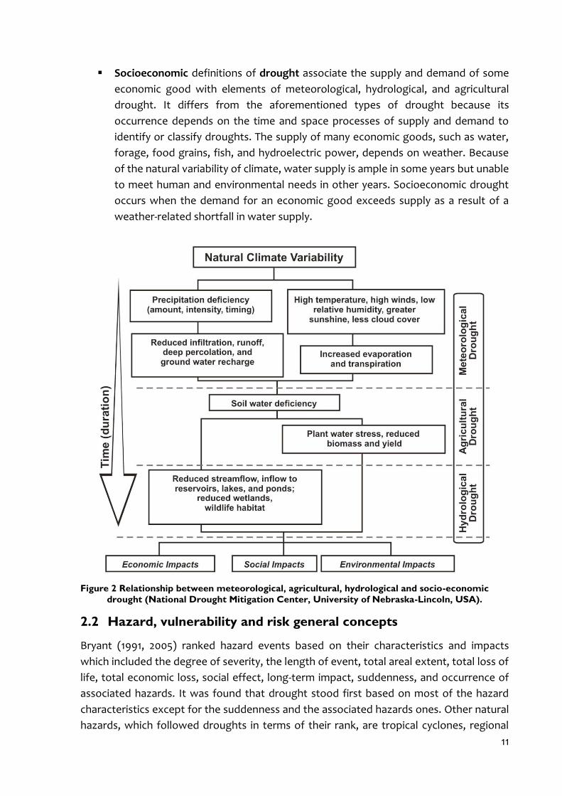
2.1.3 NDMC definition
The American National Drought Mitigation Center (NDMC) provided a way to define
drought in terms of typologies. Droughts are thus classified as meteorological,
agricultural, hydrological, and socio-economic inter-related events (see Figure 2). The
duration component of the event is the main driver of the transition process from a type
of drought to another, which implies the outbreak of various impacts.
3http://glossary.ametsoc.org/wiki/Main_Page 4http://www.unccd.int/en/about-the-convention/Pages/Text-Part-I.aspx

Definitions of drought typologies identified by the NDMC are provided in the following 4F
5:
Meteorological drought is defined usually on the basis of the degree of dryness
(in comparison to some “normal” or average amount) and the duration of the dry
period. Definitions of meteorological drought must be considered as region
specific since the atmospheric conditions that result in deficiencies of precipitation
are highly variable from region to region.
Agricultural drought links various characteristics of meteorological (or
hydrological) drought to agricultural impacts, focusing on precipitation shortages,
differences between actual and potential evapotranspiration, soil water deficits,
reduced groundwater or reservoir levels, and so forth. Plant water demand
depends on prevailing weather conditions, biological characteristics of the specific
plant, its stage of growth, and the physical and biological properties of the soil. A
good definition of agricultural drought should be able to account for the variable
susceptibility of crops during different stages of crop development, from
emergence to maturity. Deficient topsoil moisture at planting may hinder
germination, leading to low plant populations per hectare and a reduction of final
yield. However, if topsoil moisture is sufficient for early growth requirements,
deficiencies in subsoil moisture at this early stage may not affect final yield if
subsoil moisture is replenished as the growing season progresses or if rainfall
meets plant water needs.
Hydrological drought is associated with the effects of periods of precipitation
(including snowfall) shortfalls on surface or subsurface water supply (i.e.,
streamflow, reservoir and lake levels, groundwater). The frequency and severity of
hydrological drought is often defined on a watershed or river basin scale.
Although all droughts originate with a deficiency of precipitation, hydrologists are
more concerned with how this deficiency plays out through the hydrologic
system. Hydrological droughts are usually out of phase with or lag the occurrence
of meteorological and agricultural droughts. It takes longer for precipitation
deficiencies to show up in components of the hydrological system such as soil
moisture, streamflow, and groundwater and reservoir levels. As a result, these
impacts are out of phase with impacts in other economic sectors. For example, a
precipitation deficiency may result in a rapid depletion of soil moisture that is
almost immediately discernible to agriculturalists, but the impact of this deficiency
on reservoir levels may not affect hydroelectric power production or recreational
uses for many months. Also, water in hydrologic storage systems (e.g., reservoirs,
rivers) is often used for multiple and competing purposes (e.g., flood control,
irrigation, recreation, navigation, hydropower, wildlife habitat), further
complicating the sequence and quantification of impacts. Competition for water in
these storage systems escalates during drought and conflicts between water
users increase significantly.
5http://drought.unl.edu/DroughtBasics/TypesofDrought.aspx
11
Socioeconomic definitions of drought associate the supply and demand of some
economic good with elements of meteorological, hydrological, and agricultural
drought. It differs from the aforementioned types of drought because its
occurrence depends on the time and space processes of supply and demand to
identify or classify droughts. The supply of many economic goods, such as water,
forage, food grains, fish, and hydroelectric power, depends on weather. Because
of the natural variability of climate, water supply is ample in some years but unable
to meet human and environmental needs in other years. Socioeconomic drought
occurs when the demand for an economic good exceeds supply as a result of a
weather-related shortfall in water supply.
Figure 2 Relationship between meteorological, agricultural, hydrological and socio-economic
drought (National Drought Mitigation Center, University of Nebraska-Lincoln, USA).
2.2 Hazard, vulnerability and risk general concepts
Bryant (1991, 2005) ranked hazard events based on their characteristics and impacts
which included the degree of severity, the length of event, total areal extent, total loss of
life, total economic loss, social effect, long-term impact, suddenness, and occurrence of
associated hazards. It was found that drought stood first based on most of the hazard
characteristics except for the suddenness and the associated hazards ones. Other natural
hazards, which followed droughts in terms of their rank, are tropical cyclones, regional

floods, earthquakes, and volcanoes. Moreover, droughts rank first as well among all
natural hazards when measured in terms of the number of people affected (Hewitt, 1997;
Obasi, 1994).
However, even if drought as a risk has rightly deserved the attention of the scientific
community in the last decades (Dai, 2011; Heim, 2002; Mishra & Singh, 2010; William Pozzi,
Cripe, Heim, Brewer, & Sheffield, 2011; Redmond, 2002), the difficulties in the depiction of
drought risk are not lesser than those encountered in the definition of the drought itself.
2.2.1 UN/ISDR definitions
The United Nations secretariat of the International Strategy for Disaster Reduction
(UN/ISDR) defined hazard as “a potentially damaging physical event, phenomenon and/or
human activity, which may cause the loss of life or injury, property damage, social and
economic disruption or environmental degradation” 5F
6.
The potential disaster losses in terms of lives, health status, livelihoods, assets and
services, which could occur to a particular community or a society over some specified
future time period, are defined as disaster risk (UN/ISDR, 2009). The degree of
vulnerability of a region depends on the environmental and social characteristics of the
region and is measured by the inhabitants’ ability to anticipate, cope with, resist, and
recover from the occurred disaster (UN/ISDR, 2009).The risk associated with a disaster
for any region or group is a product of the exposure to the natural hazard and the
vulnerability of the society to the event. By consequence, drought risk is based on a
combination of the frequency, severity, and spatial extent of drought events (the physical
nature of the considered hazard) and the degree to which a population or activity is
vulnerable to the effects of drought (UN/ISDR, 2009).
The same agency defined the coping capacity as “a combination of all strengths and
resources available within a community or organization that can reduce the level of risk,
or the effects of a disaster” 6F
7.
2.2.2 Vulnerability and resilience
It is widely accepted that even though we are commonly dealing with vulnerability, a
unique scientific concept that describes the term has not been agreed so far (Bogardi &
Birkmann 2004, p. 75). The issue produce the following paradox: “we aim to measure
vulnerability, yet we cannot define it precisely” (Birkmann 2006, p. 11).
Various definitions of vulnerability have been proposed in literature, a selection of the
most popular ones is given in the following.
Vogel and O’Brien (2004) defined vulnerability as a multidimensional and differential
concept which is scale dependent and dynamic.
6http://www.ehs.unu.edu/elearning/mod/glossary/view.php?id=8&mode=&hook=ALL&sortkey=&sortorder=&fullsearch=0&page=1 7http://www.unisdr.org/we/inform/terminology

13
The concept of vulnerability was narrowed into a social vulnerability definition by Cannon
et. al (2003) that considers the Initial well-being of the vulnerable people, their livelihood
and resilience, the degree of self and social protection and the social, political and
institutional networks they are part of.
Another description of social vulnerability was given by Downing et al. (2006) which
involves the dynamic differential exposure to multiple stresses experienced or
anticipated by the different units exposed. Moreover they identified the root causes of
social vulnerability in the actions and multiple attributes of human actors.
Along with vulnerability comes the concept of resilience; this term describes the
capability of a system to maintain its basic functions and structures in a time of shocks
and perturbations (N. W. Adger, Arnell, & Tompkins, 2005; Allenby & Fink, 2005). Adger
(2000, p.1) defines social resilience as the ability of groups or communities to cope with
external stresses and disturbances. A system is considered resilient if it can mobilize
sufficient self-organization to maintain essential structures and processes within a coping
or adaptation process.
2.3 The emergency management
Emergency management is defined by the UN/ISDR as follows: “The organization and
management of resources and responsibilities for dealing with all aspects of
emergencies, in particularly preparedness, response and rehabilitation. Emergency
management involves plans, structures and arrangements established to engage the
normal endeavors of government, voluntary and private agencies in a comprehensive and
coordinated way to respond to the whole spectrum of emergency needs.”
Figure 3 Source: Wilhite, 1999 adapted in FAO Subregional Office for Southern and East Africa
Harare, 2004.

Another definition of the emergency cycle is given by Whilite (1999) and highlights how
the past emphasis on crisis management has meant that society has moved from one
disaster to the next without reducing the risks nor the impacts. The emergency
management was therefore reduced only to a crisis management (see lower part of
Figure 3) while nowadays the Disaster Risk Reduction (DRR) approach raised the
importance of the risk management (upper part of Figure 3) and its mitigation and
preparedness components.
The preparedness term includes the activities and measures taken in advance to ensure
effective response to the impact of hazards, including the issuance of timely and effective
early warnings and the temporary evacuation of people and property from threatened
locations. Response is defined as the provision of assistance or intervention during or
immediately after a disaster to meet the life preservation and basic subsistence needs of
those people affected. It can be of an immediate, shirt term, or protracted duration.
Rehabilitation comprises decisions and actions taken after a disaster with a view to
restoring or improving the pre-disaster living conditions of the stricken community, while
encouraging and facilitating necessary adjustments to reduce disaster risk. The mitigation
phase is often included in the emergency management cycle and it involves structural and
non-structural measures undertaken to limit the adverse impact of natural hazards,
environmental degradation and technological hazards.
The same UN agency defined disaster risk management as follows: “The systematic
process of using administrative decisions, organization, operational skills and capacities
to implement policies, strategies and coping capacities of the society and communities to
lessen the impacts of natural hazards and related environmental and technological
disasters. This comprises all forms of activities, including structural and non-structural
measures to avoid (prevention) or to limit (mitigation and preparedness) adverse effects
of hazards.” (UN/ISDR, 2004b)
2.4 Early warning systems
Early warning systems are part of the preparedness phase, and were defined by the
International Strategy for Disaster Reduction (UN/ISDR) in 2006 as “the provision of
timely and effective information, through identified institutions, that allows individuals
exposed to hazard to take action to avoid or reduce their risk and prepare for effective
response”. Those systems are the integration of four main elements:
I. Risk Knowledge: comprehensive multi risk assessments provide essential
information to set priorities both for mitigation and prevention strategies and for
designing early warning systems.
II. Monitoring and Predicting: systems with these capabilities provide timely
estimates of the potential risk faced by communities, economies and the
environment.
III. Dissemination: communication systems are needed for delivering warning
messages to the potentially affected communities. The messages need to be
15
reliable, synthetic and simple to be understood both by authorities and general
public.
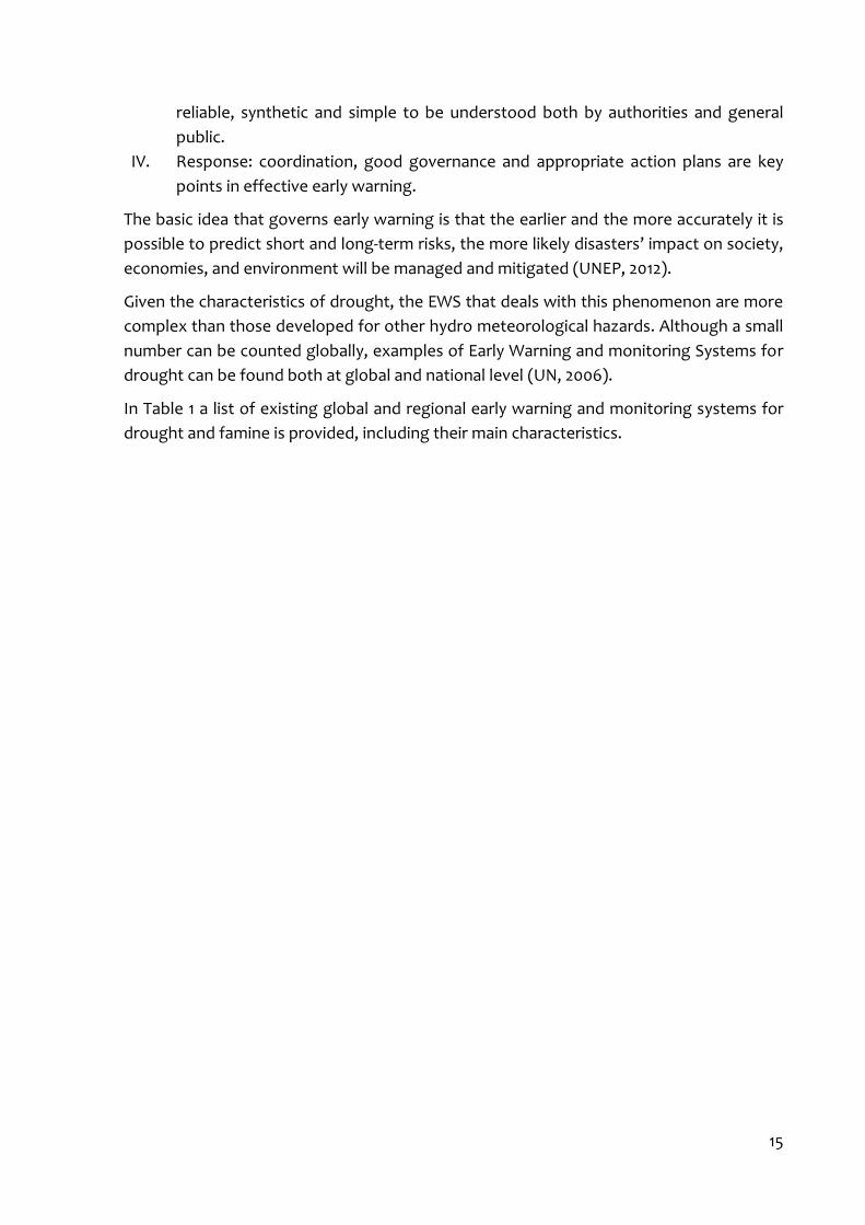
IV. Response: coordination, good governance and appropriate action plans are key
points in effective early warning.
The basic idea that governs early warning is that the earlier and the more accurately it is
possible to predict short and long-term risks, the more likely disasters’ impact on society,
economies, and environment will be managed and mitigated (UNEP, 2012).
Given the characteristics of drought, the EWS that deals with this phenomenon are more
complex than those developed for other hydro meteorological hazards. Although a small
number can be counted globally, examples of Early Warning and monitoring Systems for
drought can be found both at global and national level (UN, 2006).
In Table 1 a list of existing global and regional early warning and monitoring systems for
drought and famine is provided, including their main characteristics.
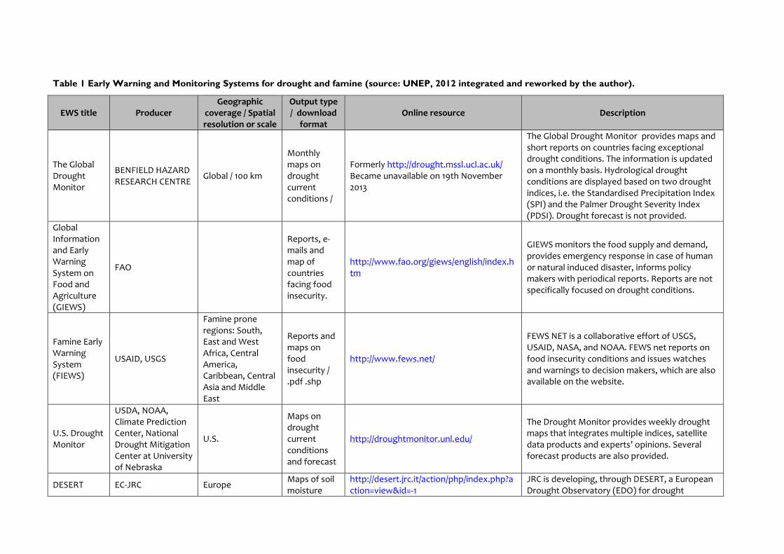
Table 1 Early Warning and Monitoring Systems for drought and famine (source: UNEP, 2012 integrated and reworked by the author).
EWS title Producer Geographic
coverage / Spatial resolution or scale
Output type / download
format Online resource Description
The Global Drought Monitor
BENFIELD HAZARD RESEARCH CENTRE
Global / 100 km
Monthly maps on drought current conditions /
Formerly http://drought.mssl.ucl.ac.uk/ Became unavailable on 19th November 2013
The Global Drought Monitor provides maps and short reports on countries facing exceptional drought conditions. The information is updated on a monthly basis. Hydrological drought conditions are displayed based on two drought indices, i.e. the Standardised Precipitation Index (SPI) and the Palmer Drought Severity Index (PDSI). Drought forecast is not provided.
Global Information and Early Warning System on Food and Agriculture (GIEWS)
FAO
Reports, e-mails and map of countries facing food insecurity.
http://www.fao.org/giews/english/index.htm
GIEWS monitors the food supply and demand, provides emergency response in case of human or natural induced disaster, informs policy makers with periodical reports. Reports are not specifically focused on drought conditions.
Famine Early Warning System (FIEWS)
USAID, USGS
Famine prone regions: South, East and West Africa, Central America, Caribbean, Central Asia and Middle East
Reports and maps on food insecurity / .pdf .shp
http://www.fews.net/
FEWS NET is a collaborative effort of USGS, USAID, NASA, and NOAA. FEWS net reports on food insecurity conditions and issues watches and warnings to decision makers, which are also available on the website.
U.S. Drought Monitor
USDA, NOAA, Climate Prediction Center, National Drought Mitigation Center at University of Nebraska
U.S.
Maps on drought current conditions and forecast
http://droughtmonitor.unl.edu/
The Drought Monitor provides weekly drought maps that integrates multiple indices, satellite data products and experts’ opinions. Several forecast products are also provided.
DESERT EC-JRC Europe Maps of soil moisture
http://desert.jrc.it/action/php/index.php?action=view&id=-1
JRC is developing, through DESERT, a European Drought Observatory (EDO) for drought

17
EWS title Producer Geographic
coverage / Spatial resolution or scale
Output type / download
format Online resource Description
forecasting, assessment and monitoring. DESERT currently provides freely daily soil moisture maps of Europe, precipitation, vegetation and response maps.
Food Security Situation Maps
Food Security and Nutrition Group (FSNWG)
East Africa
Food security maps and monthly updates / .pdf
http://www.disasterriskreduction.net/east-central-africa/fsnwg/en/
FSNWG provides a platform for Disaster Risk Reduction in the region.

2.5 Drought and food security
Measuring the effects of a disaster implies firstly the identification and definition of what
those effects are. The case of drought, a slow onset complex disaster, poses another
challenge with this respect. As Peduzzi et al. stated in 2009, casualties normally attributed
to droughts are typically caused by food insecurity rather than by the natural
phenomenon itself. Previous studies (Birkmann & Mucke, 2011; Peduzzi et al., 2009)
dealing with drought risk had pointed out that the estimation of affected people is highly
complex and inaccurate to some extent compared to that of other natural disasters. In
fact drought disasters typically involve a high proportion of indirect losses (Economic
Commission for Latin America and the Caribbean & the World Bank, 2003). The high share
of indirect losses of the total losses and the lack of visible damage outside the agriculture
sector can lead to the undervaluation of the overall impacts of drought (Below et al.,
2007). This is the case of drought-related mortality, for example, which is caused by
drought impacts on livelihoods, contributing to reduce food intake, exacerbate
migration, and creation of water and sanitation problems, leading to deterioration of
health conditions, augmenting diseases, and eventually death (de Waal, 1989). As a
matter of fact drought has accounted for the majority of the food shortages and food aid
relief operations undertaken in the world since the 1980s (Minamiguchi, 2005). Official
national statistics of drought affected population are often unavailable or based on
different assumptions, which causes data to be hardly comparable in the absence of a
common assessment framework. It should also be noted that emergency operations are
put in place when food crisis occur, therefore the availability of a food security alert
would be of help in the preparedness and response phases. In conclusion the food
security status is chosen, in this study, as the ultimate indirect outcome of a drought
event and thus it is investigated in order to be modeled starting from an environmental
hazard assessment.
The food security condition of any households or individuals is the outcome of the
interaction of a broad range of agro-environmental, socio-economic and biological
factors. Therefore there is no single, direct measure of food security (WFP, 2009). A
variety of proxy exists at the individual, household and national level in support of food
security measurement that remains, however, an elusive concept difficult to be measured
(Barrett, 2010). It has been pointed out by Peduzzi et al. (2009) that food security is not
to be intended as a hazard itself, being sometimes human-induced, even if it is the main
cause of the casualties following a drought event. The concept of food security, as it is
widely accepted, rests on three pillars: availability, access, and utilization of food. These
concepts are hierarchical, i.e. availability is necessary but not sufficient to ensure access,
which is, in turn, necessary but not sufficient for effective utilization (Webb et al., 2006).
As Nobel Laureate Amartya Sen wrote, “starvation is the characteristic of some people
not having enough food to eat. It is not the characteristic of there being not enough food
to eat. While the latter can be a cause of the former, it is but one of many possible
causes” (Sen, 1981).

19
In the frame of this study only the availability of and the access to food were taken into
consideration, the first analyzed with indicators for crop production anomalies and the
second modeled considering physical accessibility to markets.
The rationale for the conception of the present vulnerability model is the possibility of
producing food security outlooks without using field surveys, which are normally part of a
comprehensive vulnerability and food security assessment. In Figure 4 a workflow
representing a typical vulnerability assessment framework is presented. Unlike a
comprehensive vulnerability assessment, the present vulnerability model starts from the
hazard, i.e. the monitoring of the agro-ecological conditions (highlighted in yellow in
Figure 4), and will use food availability retrieved at the household level as validation data
(highlighted in light violet in Figure 4). The objective of the vulnerability model is thus to
represent spatial relations and interactions between agricultural affected areas and
impacted population.
Figure 4 The Food and Nutrition Security conceptual framework (source: WFP, 2009).

2.6 ITHACA vegetation anomaly monitoring system
ITHACA developed a system for the early detection and monitoring of vegetation stress
and agricultural drought events on a global scale. The system mainly relies on satellite
derived data.
ITHACA system is based on the near real-time monitoring of a selection of vegetation
indexes that allows the early detection of vegetation water stress conditions. That is, the
monitoring of phenological parameters allows the assessment of the current vegetation
productivity and its projection at the end of the growing season (Bellone, Boccardo, &
Perez, 2009).
The aim of the system is the timely detection of critical conditions in vegetation health
and productivity, during a vegetative growing season and at its end. By consequence the
system can pinpoint agricultural areas with increased crop or pasture failure thus
enabling end-users to better plan the interventions.
Currently, the development of a webGIS service suitable for the visualization and
distribution of final monitoring products (near real-time and historical maps) is ongoing.
2.6.1 Data input and methodology
Vegetation monitoring procedures are based on extracting and elaborating, for each
considered vegetation growing season (see Figure 5), a set of phenological parameters
from the yearly NDVI function (the regular curve depicted in Figure 5) that best fits the
original yearly NDVI time-series (the irregular curve depicted in Figure 5).
The vegetation phenology concerns the annual green-up, or growth, and senescence
cycles of plants. Seasonal changes observed in NDVI time-series have proven useful in
tracking land surface phenology and vegetation development stages, and for mapping
vegetation dynamics. Specifically, produced datasets are based on the following
phonological parameters:
the Start of the Season: time when the left edge of the NDVI fitted function
outreaches a user-defined threshold, that corresponds to the left minimum level
(point A in Figure 5). This is the time at which seasonal photosynthetic activity
begins;
the Seasonal Small Integral: integral of the NDVI function describing the season
from the Start of the Season to the End of the Season (the grey area between the
fitted function and the base level, area H, in Figure 5).
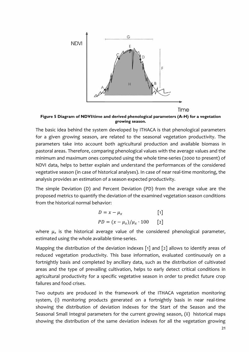
21
Figure 5 Diagram of NDVI/time and derived phenological parameters (A-H) for a vegetation
growing season.
The basic idea behind the system developed by ITHACA is that phenological parameters
for a given growing season, are related to the seasonal vegetation productivity. The
parameters take into account both agricultural production and available biomass in
pastoral areas. Therefore, comparing phenological values with the average values and the
minimum and maximum ones computed using the whole time-series (2000 to present) of
NDVI data, helps to better explain and understand the performances of the considered
vegetative season (in case of historical analyses). In case of near real-time monitoring, the
analysis provides an estimation of a season expected productivity.
The simple Deviation (D) and Percent Deviation (PD) from the average value are the
proposed metrics to quantify the deviation of the examined vegetation season conditions
from the historical normal behavior:
[1]
[2]
where μx is the historical average value of the considered phenological parameter,
estimated using the whole available time-series.
Mapping the distribution of the deviation indexes [1] and [2] allows to identify areas of
reduced vegetation productivity. This base information, evaluated continuously on a
fortnightly basis and completed by ancillary data, such as the distribution of cultivated
areas and the type of prevailing cultivation, helps to early detect critical conditions in
agricultural productivity for a specific vegetative season in order to predict future crop
failures and food crises.
Two outputs are produced in the framework of the ITHACA vegetation monitoring
system, (i) monitoring products generated on a fortnightly basis in near real-time
showing the distribution of deviation indexes for the Start of the Season and the
Seasonal Small Integral parameters for the current growing season, (ii) historical maps
showing the distribution of the same deviation indexes for all the vegetation growing

seasons included in the 2000-2012 years (2 seasons/year, that is 2 maps/year). A
description of the cited products follows.
The Seasonal Small Integral PD imagery describes vegetation condition for the main and
secondary growing seasons for the years 2000 to present (two images per year) using the
Seasonal Small Integral parameter extracted from MODIS NDVI time-series. Figure 6
shows, for instance, the distribution of the PDs (see equation [2]) for the selected
phenological parameter, estimated on a pixel basis (0.05 degrees). In addition, in order to
provide a more effective display of the most affected areas, raw results are also
aggregated at the second level administrative boundary (Figure 7), according to a higher
frequency distribution rule. As an example, in the maps reported in in Figure 6 and in
Figure 7, areas where the Seasonal Small Integral parameter for the examined vegetation
season has a negative deviation from the average value are shown using light orange to
red colors.
It should be noted that the considered growing seasons, for the different areas of the
world, refer to different months in the year, according to the specific agro-climatic
zoning. For areas with two different seasons in their vegetation/crop calendar, mapped
Small Integral PDs for main and secondary seasons refer respectively to the first and
second season encountered from the start of the considered year; for the areas where a
unique growing season is detected, only the first season is mapped (i.e. in the second
season image these areas are indicated as areas where no growing season has been
detected during the analyses). Besides, in the output imagery, barren areas, urban and
built-up areas, evergreen/deciduous needle leaf/broadleaf forest areas, swamp
vegetation, water bodies, and, in general, areas where no growing season has been
detected during the analyses, are excluded from the analyses and given a specific fill
value.
Moreover, raw imagery (0.05 degrees) showing the distribution of the original Seasonal
Small Integer parameter (Raw Seasonal Small Integral imagery) for examined areas for the
main and secondary growing seasons (for 2000 to present; 2 images per year) are also
produced in order to allow direct vegetation productivity comparisons between two or
more growing seasons specifically selected by end-users.

23
Figure 6 Pixel based output of the Percent Deviations (PDs) of the phenological parameter
Seasonal Small Integral for the 2011 growing season for the Sahel area.
Figure 7 Aggregated on the second level administrative boundary output of the Percent
Deviations (PDs) of the phenological parameter Seasonal Small Integral for the 2011 growing
season for the Sahel area.
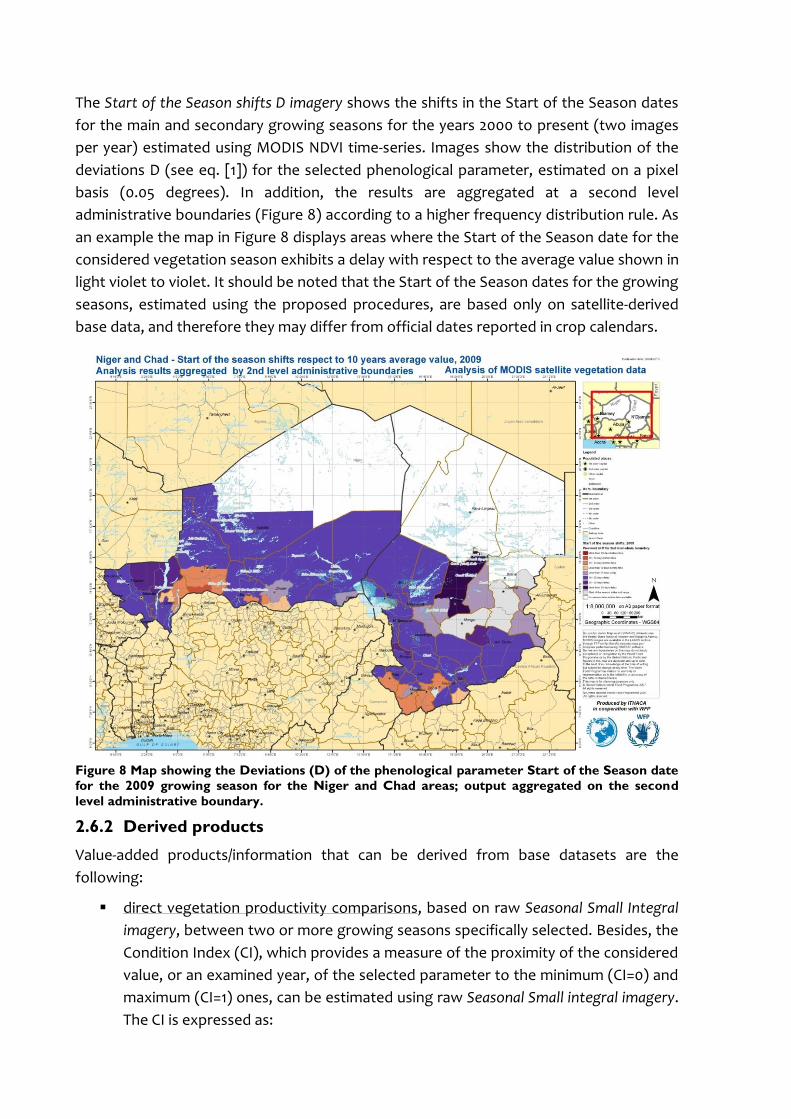
The Start of the Season shifts D imagery shows the shifts in the Start of the Season dates
for the main and secondary growing seasons for the years 2000 to present (two images
per year) estimated using MODIS NDVI time-series. Images show the distribution of the
deviations D (see eq. [1]) for the selected phenological parameter, estimated on a pixel
basis (0.05 degrees). In addition, the results are aggregated at a second level
administrative boundaries (Figure 8) according to a higher frequency distribution rule. As
an example the map in Figure 8 displays areas where the Start of the Season date for the
considered vegetation season exhibits a delay with respect to the average value shown in
light violet to violet. It should be noted that the Start of the Season dates for the growing
seasons, estimated using the proposed procedures, are based only on satellite-derived
base data, and therefore they may differ from official dates reported in crop calendars.
Figure 8 Map showing the Deviations (D) of the phenological parameter Start of the Season date
for the 2009 growing season for the Niger and Chad areas; output aggregated on the second
level administrative boundary.
2.6.2 Derived products
Value-added products/information that can be derived from base datasets are the
following:
direct vegetation productivity comparisons, based on raw Seasonal Small Integral
imagery, between two or more growing seasons specifically selected. Besides, the
Condition Index (CI), which provides a measure of the proximity of the considered
value, or an examined year, of the selected parameter to the minimum (CI=0) and
maximum (CI=1) ones, can be estimated using raw Seasonal Small integral imagery.
The CI is expressed as:

25
[3]
where
x is the value of the phenological parameter for the examined growing season;
minx and maxx are the minimum and maximum values of the parameter
considered, extracted from the whole available historical time-series (2000 to
present).
drought historical products, that is the investigation of the historical occurrence of
vegetation stress events in a region through the aggregation of the Seasonal Small
Integral Percent Deviation values for selected years. This analysis allows the
identification of the areas showing the greatest number of negative vegetation
productivity deviations in subsequent growing seasons. For instance, areas most
affected by poor vegetation growth in the selected time interval could be
considered more vulnerable in case of future drought events (Figure 9). This
dataset allows drought hazard identification, which is a required step in drought
risk assessment and identification. Refinement though is possible by coupling
historical vegetation productivity information with ancillary data, such as the
distribution of cultivated areas and the type of prevailing cultivation, or the
livelihood zones distribution.
Figure 9 Map showing the number of negative vegetation productivity deviations between 2006
and 2010 in the Sahel area.

3 LITERATURE REVIEW
In this chapter a review of inspiring works is reported: (i) the existing drought monitoring
and early warning systems that integrate vulnerability in one of its forms; and (ii)
attempts and suggestions on what vulnerability for drought risk calculation should
include. The focus of the present chapter is not to provide a list of existing drought EW
and monitoring system and indexes to calculate drought hazard, but to examine the
studies that targeted vulnerability as a key factor in drought risk measurement.
The category (i) includes global systems that are both drought specific and multi-risk.
At first place the WorldRiskIndex, developed by the United Nations University Institute
for Environment and Human Security (Bonn, Germany), should be mentioned. The
WorldRiskIndex indicates, for each country, the probability that this will be affected by a
disaster. Globally available data are used to calculate the disaster risk for the countries
analyzed. In the framework of the WorldRiskIndex, disaster risk is conceived as
interactions among natural hazards and social, political and environmental factors. This
index, in addition to exposure analysis, focuses on the vulnerability of the population,
which is subdivided into susceptibility, capacities to cope with and to adapt to future
natural disasters. The risk is then seen as a function of exposure and vulnerability and is
calculated per aggregation at country level. The WorldRiskIndex consists of indicators
subdivided into four components (Figure 10): exposure to natural hazards (i.e.
earthquakes, storms, floods, droughts and sea level rise); susceptibility (i.e. a function of
public infrastructure, housing conditions, nutrition and the general country economic
status); coping capacities (i.e. a function of governance, disaster preparedness and early
warning, medical services, social and economic security); and adaptive capacities to
future natural disasters (Birkmann & Mucke, 2011). The World Risk Report provides a
global ranking of the country risk index and a detailed description of the applied
methodology and data used (Birkmann & Mucke, 2011).
Figure 10 Scheme of the concept of the WorldRiskIndex (source: Birkmann & Mucke, 2011).
Although aiming at mapping the risk globally (see Figure 11), the World Risk Report
reports a case study on a sub-national level (i.e. Indonesia case study). It must be
mentioned that, in the calculation of exposure, drought exposed individuals as retrieved

27
by CRED EM-DAT database, were only half-weighted, with respect to other hazards, due
to the peculiarity of the drought hazard in showing its effects. The latter assumption,
according to the author, justifies the present attempt to concentrate on single hazard risk
models, especially for drought.
Figure 11 WorldRiskIndex as result of the exposure and vulnerability (source: Birkmann &
Mucke, 2011).
The WorldRiskIndex was certainly inspired by the work of Peduzzi et al. (2009) which was
equally aimed at conceiving a worldwide valid multi risk index, i.e. the Disaster Risk Index
(DRI), to the profit of the United Nations Development Programme (UNDP). The
mandate from UNDP was actually to analyze potential links between vulnerability to
natural hazards and levels of development of nations. The DRI was the first model to
prove a statistical evidence of the mentioned link at the global scale. The DRI takes into
account, among the others, the drought risk, which is calculated considering the
following indicators: physical exposure, Gross Domestic Product (GDP) per capita and the
percentage of arable land; the last two indicators accounts for vulnerability in the DRI
model for drought.
Among the few existing global drought specific monitoring system a well renowned one
is the Fews Net (Famine Early Warning Systems Network) project7F
8. The Fews Net is a
provider of early warning and analysis on acute food insecurity. In order to do so it
constantly monitors vegetation and meteorological drought indicators (satellite-based)
and couples them with field survey data such as those relative to markets and trade and
nutrition. The Fews Net provides food security assessments and outlooks on the basis of
projected likely scenarios. These outputs are provided at subnational levels for a set of
countries food-insecurity prone or otherwise strategic. The most useful characteristic of
those food security assessments and outlooks is the fact that they are classified
according to a widely recognized frame of classification, i.e. the Integrated Food Security
Phase Classification (IPC 2.0) 8F
9 scale, that allows the data to be easily understandable by a
8 http://www.fews.net/ 9 http://www.fews.net/our-work/our-work/integrated-phase-classification

wide public of operators and users (for more details on the IPC scale refer to paragraph
4.4.1) and comparable among countries.
Figure 12 Few Net food security outlook, near and medium term, for Ethiopia (source
www.fewsnet.net accessed on February 18th 2014).
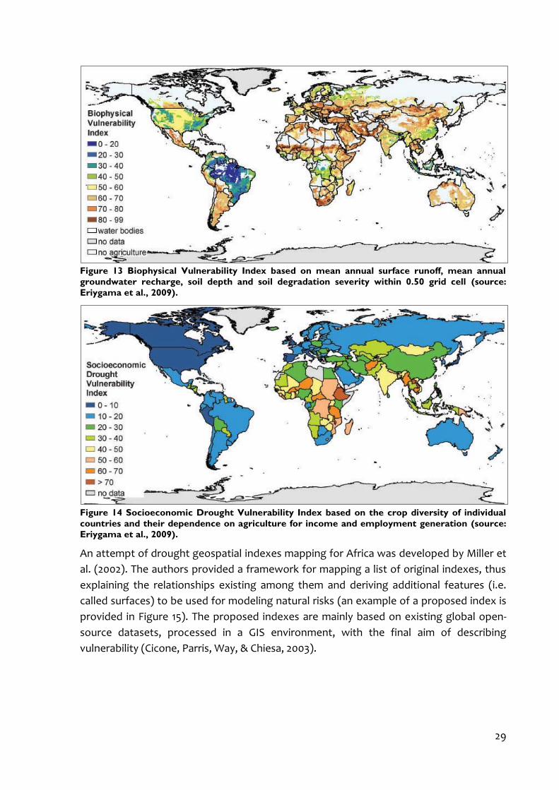
An original work on drought mapping was realized by Eriygama et al. (2009), which arose
from the observation that a scarcity of attempts to extensively describe and represent
various aspects and impacts of drought, as an independent natural disaster and as a
global complex phenomenon, exist. The work contains a review of quite a large set of
indexes of both drought hazard and types of vulnerability to drought; these indexes were
mapped by the authors at a global extent when possible on a 0.5 grid cell basis, or
aggregated at country level. Of particular interest are the vulnerability indexes that are
proposed, one per each of the drought vulnerability aspects (i.e. infrastructure,
biophysical and socioeconomic vulnerability indexes). Two examples of drought
vulnerability indexes mapped are provided in Figure 13 and in Figure 14. The study
concluded that more effort should be put in quantifying and indexing vulnerability
globally, with a view also of considering climate change in the medium and long run.
29
Figure 13 Biophysical Vulnerability Index based on mean annual surface runoff, mean annual
groundwater recharge, soil depth and soil degradation severity within 0.50 grid cell (source:
Eriygama et al., 2009).
Figure 14 Socioeconomic Drought Vulnerability Index based on the crop diversity of individual
countries and their dependence on agriculture for income and employment generation (source:
Eriygama et al., 2009).
An attempt of drought geospatial indexes mapping for Africa was developed by Miller et
al. (2002). The authors provided a framework for mapping a list of original indexes, thus
explaining the relationships existing among them and deriving additional features (i.e.
called surfaces) to be used for modeling natural risks (an example of a proposed index is
provided in Figure 15). The proposed indexes are mainly based on existing global open-
source datasets, processed in a GIS environment, with the final aim of describing
vulnerability (Cicone, Parris, Way, & Chiesa, 2003).
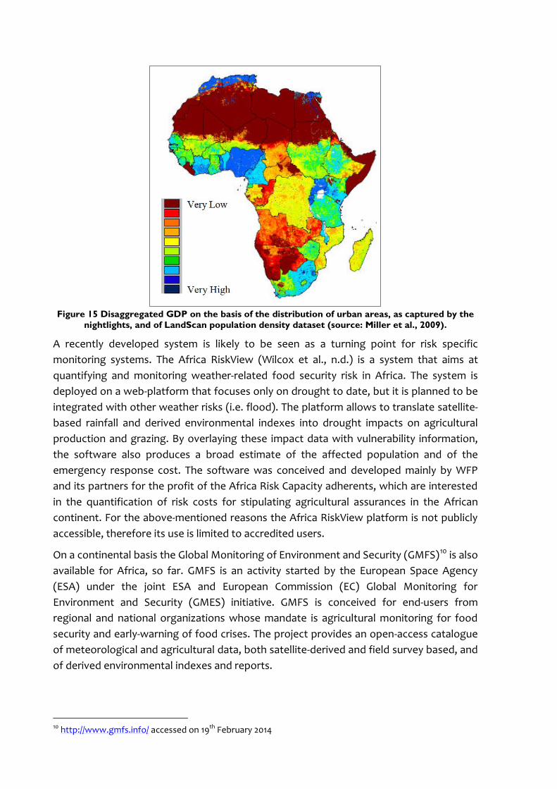
Figure 15 Disaggregated GDP on the basis of the distribution of urban areas, as captured by the
nightlights, and of LandScan population density dataset (source: Miller et al., 2009).
A recently developed system is likely to be seen as a turning point for risk specific
monitoring systems. The Africa RiskView (Wilcox et al., n.d.) is a system that aims at
quantifying and monitoring weather-related food security risk in Africa. The system is
deployed on a web-platform that focuses only on drought to date, but it is planned to be
integrated with other weather risks (i.e. flood). The platform allows to translate satellite-
based rainfall and derived environmental indexes into drought impacts on agricultural
production and grazing. By overlaying these impact data with vulnerability information,
the software also produces a broad estimate of the affected population and of the
emergency response cost. The software was conceived and developed mainly by WFP
and its partners for the profit of the Africa Risk Capacity adherents, which are interested
in the quantification of risk costs for stipulating agricultural assurances in the African
continent. For the above-mentioned reasons the Africa RiskView platform is not publicly
accessible, therefore its use is limited to accredited users.
On a continental basis the Global Monitoring of Environment and Security (GMFS)9F
10 is also
available for Africa, so far. GMFS is an activity started by the European Space Agency
(ESA) under the joint ESA and European Commission (EC) Global Monitoring for
Environment and Security (GMES) initiative. GMFS is conceived for end-users from
regional and national organizations whose mandate is agricultural monitoring for food
security and early-warning of food crises. The project provides an open-access catalogue
of meteorological and agricultural data, both satellite-derived and field survey based, and
of derived environmental indexes and reports.
10 http://www.gmfs.info/ accessed on 19th February 2014

31
Concerning food security indicators and mapping, interesting national case studies have
been proposed by the NASA Socioeconomic Data and Applications Center (SEDAC)10F
11. The
purpose of the work (i.e. Poverty and Food Security Case Studies) was to provide high
spatial resolution subnational estimates of poverty and food security (see a case study
example for Kenya in Figure 16). The availability of data is limited to a few numbers of
case studies and is not up to date, having the project ended in 2002.
Figure 16 The map shows the number of poor people per km2 in the Kenya Kajiado district of
Kenya (source: International Livestock Research Institute, 20040115, Kenya Kajiado Case Study:
ILRI, Nairobi).
Other suggestions for drought risk indicators were found in the work of Julich (2006)
which was focused on drought impact assessment on households. The author states that
the origin of disparities in drought vulnerability resides in the household level. Examples
of proposed, but non applied, indicators are the diversity of crops and the number of
economical active persons in relation to total household components.
A useful inventory of drought national warning and mitigation systems for Africa was
provided by Nyabeze (2012) in the framework of the project “improved Drought Early
Warning and FORecasting to strengthen preparedness and adaptation to droughts in
Africa” (DEWFORA)11F
12. The inventory covers a dozen countries of Western, Eastern and
Southern Africa, for each of those providing a description of local warning indicators for
11 http://sedac.ciesin.columbia.edu/data/set/povmap-poverty-food-security-case-studies accessed on 19th February 2014 12 http://www.dewfora.net

drought as well as institutional ones. In the framework of the same EU-funded project an
interesting report is found on the definition of a methodology for assessing drought
vulnerability across Africa (Garrote, 2012). It is there stated that “…in the context of a
drought early warning system, the focus on vulnerability may prove to be very effective
since it includes the evaluation of the capacity to anticipate and compensate the adverse
effects of drought.” (Garrote, 2012). The importance of defining drought indicators that
are tailored on the type of drought impact which has to be analyzed is also reported in
the document; the statement furnished to the author of the present study a valid
argument for investigating vulnerability to be coupled with a specific early warning
system.

33
4 DATA AND METHODS
In this chapter the data and the methodology used to implement the proposed
vulnerability model are presented. The first two paragraphs are devoted to a detailed
description of the datasets and of the components of the model. The third paragraph
provides an analysis of the case studies to which the model was applied. The fourth
paragraph presents the data, qualitative and quantitative, used to perform an evaluation
of the outcomes of the model applied to the selected case studies.
4.1 Data inventory
A variety of data were investigated for the purpose of the present study. A literature
research was performed in order to identify datasets used for existing early warning
systems and risk models. A data review was needed to analyze data characteristics and
their fit to use in the presented study. In particular the reference data catalogue realized
in the framework of the European Commission GMES initial operations was extensively
used (Boccardo et al., 2012).
Only a subset of datasets that had been contemplated in the first place was eventually
used for building the model indicators. Investigated datasets belong to the following
main categories:
Land Cover
Administrative boundaries
Water and agriculture
Hydrography
Elevation
Population
Development
Considering the aims of the present work and of the ITHACA drought monitoring system
itself, two requirements were considered essentials for a dataset to be selected: the
global extent and the absence of access and use constraints.
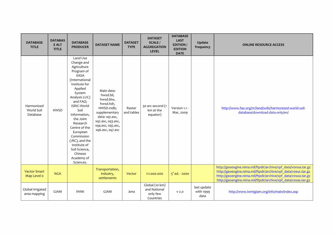
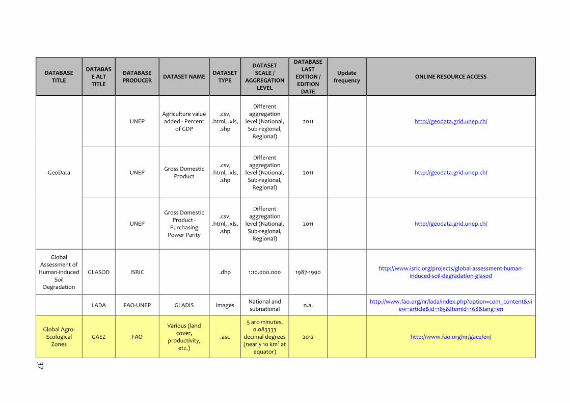
The Table 2 resumes the main characteristics of the dataset investigated for the proposed
simplified vulnerability model. Highlighted in light yellow the datasets that were
eventually considered appropriate for building the indicators of the proposed model.

Table 2 Data description.
DATABASE TITLE
DATABASE ALT TITLE
DATABASE PRODUCER
DATASET NAME DATASET
TYPE
DATASET SCALE /
AGGREGATION LEVEL
DATABASE LAST
EDITION / EDITION
DATE
Update frequency
ONLINE RESOURCE ACCESS
World Income Inequality Database
WIID UNU-WIDER
National V2.0c May
2008 http://www.wider.unu.edu/research/Database/en_GB/database/
CIA World Factbook
CIA
.pdf, .jpg, and
textual National
weekly
https://www.cia.gov/library/publications/the-world-factbook/index.html
CountrySTAT
FAO various (e.g food production, land
cover, etc.) .xls
Administrative level 1
yearly or less frequently
http://www.fao.org/economic/ess/CountrySTAT/en/
http://www.CountrySTAT.org/default.aspx
FaoSTAT
FAO
various (e.g food production, trade, food
balance)
.xls National
yearly or less frequently
LandScan Global
Population 2008 Database
LandScan 2008
Oak Ridge National
Laboratory (ORNL) for the United States
Department of Defense
United States Bureau of the
Census; National Geospatial-Intelligence
Agency (NGA); The Global
Administrative Unit Layers
(GAUL) dataset, implemented by FAO within the EC FAO Food Security for
Action Programme.
Raster (ESRIgrid)
Cell size: 0.008333333
degrees (nearly 1 km2 at equator,
30 arc-sec)
2009
http://www.ornl.gov/sci/landscan/
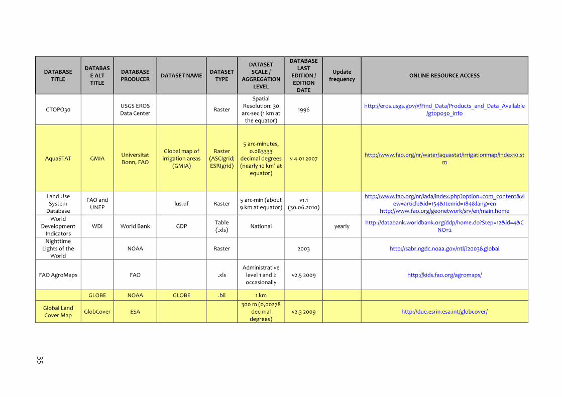
35
DATABASE TITLE
DATABASE ALT TITLE
DATABASE PRODUCER
DATASET NAME DATASET
TYPE
DATASET SCALE /
AGGREGATION LEVEL
DATABASE LAST
EDITION / EDITION
DATE
Update frequency
ONLINE RESOURCE ACCESS
GTOPO30
USGS EROS Data Center
Raster
Spatial Resolution: 30 arc-sec (1 km at
the equator)
1996
http://eros.usgs.gov/#/Find_Data/Products_and_Data_Available/gtopo30_info
AquaSTAT GMIA Universitat Bonn, FAO
Global map of irrigation areas
(GMIA)
Raster (ASCIgrid; ESRIgrid)
5 arc-minutes, 0.083333
decimal degrees (nearly 10 km2 at
equator)
v 4.01 2007
http://www.fao.org/nr/water/aquastat/irrigationmap/index10.stm
Land Use System
Database
FAO and UNEP
lus.tif Raster 5 arc-min (about 9 km at equator)
v1.1 (30.06.2010)
http://www.fao.org/nr/lada/index.php?option=com_content&view=article&id=154&Itemid=184&lang=en
http://www.fao.org/geonetwork/srv/en/main.home
World Development
Indicators WDI World Bank GDP
Table (.xls)
National
yearly http://databank.worldbank.org/ddp/home.do?Step=12&id=4&C
NO=2
Nighttime Lights of the
World
NOAA
Raster
2003
http://sabr.ngdc.noaa.gov/ntl/?2003&global
FAO AgroMaps
FAO
.xls Administrative
level 1 and 2 occasionally
v2.5 2009
http://kids.fao.org/agromaps/
GLOBE NOAA GLOBE .bil 1 km
Global Land Cover Map
GlobCover ESA
300 m (0,00278 decimal
degrees) v2.3 2009
http://due.esrin.esa.int/globcover/
DATABASE TITLE
DATABASE ALT TITLE
DATABASE PRODUCER
DATASET NAME DATASET
TYPE
DATASET SCALE /
AGGREGATION LEVEL
DATABASE LAST
EDITION / EDITION
DATE
Update frequency
ONLINE RESOURCE ACCESS
Harmonized World Soil Database
HWSD
Land Use Change and Agriculture Program of
IIASA (International Institute for
Applied System
Analysis LUC) and FAO;
ISRIC-World Soil
Information, the Joint Research
Centre of the European
Commission (JRC), and the
Institute of Soil Science,
Chinese Academy of
Sciences.
Main data: hwsd.bil,
hwsd.blw, hwsd.hdr,
HWSD.mdb; supplementary data: sq1.asc,
sq2.asc, sq3.asc, sq4.asc, sq5.asc, sq6.asc, sq7.asc
Raster and tables
30 arc-second (1 km at the equator)
Version 1.1 - Mar, 2009
http://www.fao.org/nr/land/soils/harmonized-world-soil-database/download-data-only/en/
Vector Smart Map Level 0
NGA
Transportation, industry,
settlements Vector 1:1.000.000 5° ed. - 2000
http://geoengine.nima.mil/ftpdir/archive/vpf_data/v0noa.tar.gz http://geoengine.nima.mil/ftpdir/archive/vpf_data/v0eur.tar.gz http://geoengine.nima.mil/ftpdir/archive/vpf_data/v0soa.tar.gz http://geoengine.nima.mil/ftpdir/archive/vpf_data/v0sas.tar.gz
Global Irrigated area mapping
GIAM IWMI GIAM .kmz
Global (10 km) and National
only few Countries
v 2.0 last update with 1999
data http://www.iwmigiam.org/info/main/index.asp
37
DATABASE TITLE
DATABASE ALT TITLE
DATABASE PRODUCER
DATASET NAME DATASET
TYPE
DATASET SCALE /
AGGREGATION LEVEL
DATABASE LAST
EDITION / EDITION
DATE
Update frequency
ONLINE RESOURCE ACCESS
GeoData
UNEP
Agriculture value added - Percent
of GDP
.csv, .html, .xls,
.shp
Different aggregation
level (National, Sub-regional,
Regional)
2011
http://geodata.grid.unep.ch/
UNEP
Gross Domestic Product
.csv, .html, .xls,
.shp
Different aggregation
level (National, Sub-regional,
Regional)
2011
http://geodata.grid.unep.ch/
UNEP
Gross Domestic Product -
Purchasing Power Parity
.csv, .html, .xls,
.shp
Different aggregation
level (National, Sub-regional,
Regional)
2011
http://geodata.grid.unep.ch/
Global Assessment of
Human-induced Soil
Degradation
GLASOD ISRIC
.dhp 1:10.000.000 1987-1990
http://www.isric.org/projects/global-assessment-human-induced-soil-degradation-glasod
LADA FAO-UNEP GLADIS Images
National and subnational
n.a.
http://www.fao.org/nr/lada/index.php?option=com_content&view=article&id=185&Itemid=168&lang=en
Global Agro-Ecological
Zones GAEZ FAO
Various (land cover,
productivity, etc.)
.asc
5 arc-minutes, 0.083333
decimal degrees (nearly 10 km2 at
equator)
2012
http://www.fao.org/nr/gaez/en/

DATABASE TITLE
DATABASE ALT TITLE
DATABASE PRODUCER
DATASET NAME DATASET
TYPE
DATASET SCALE /
AGGREGATION LEVEL
DATABASE LAST
EDITION / EDITION
DATE
Update frequency
ONLINE RESOURCE ACCESS
Africover
FAO
Multipurpose Landcover database
.shp 1:200.000
2002 (on Landsat
1994-1999 data)
http://www.africover.org/system/user/user.php?PHPSESSID=c1c
a6e93b412b75ae4b8e6175962b780
Towns .shp 1:100.000 2002
http://www.fao.org/geonetwork/srv/en/main.home
Global ADMinistrative
Areas GADM
Different US universities and
research institutes
Global Administrative
Areas - gadm_v1_lev0,
Global Administrative
Areas - gadm_v1_lev1
.shp n/a v 2.0/January
2012 Continuous http://www.gadm.org/
Global Administrative
Unit Layers GAUL
The GAUL is an initiative
implemented by FAO within the EC-FAO Food
Security Programme
funded by the European
Commission
g2008_2006_1
(Level1);
g2008_20006_2 (Level2) (global
datasets). Lower levels (level 3, level
4, level5), when available, are supplied on
individual country base.
.shp GAUL
2009/2009 Yearly http://www.fao.org/geonetwork/srv/en/main.home;
39
4.2 Conceptual model
The challenge of the present work mainly resides in the measurement of the vulnerability
that has to be coupled with drought hazard values (Angeluccetti & Perez, 2013). As stated
in 2006 by Birkmann, the concept of vulnerability is multidimensional and often ill-
defined, therefore it is difficult to define a universal measurement methodology or to
reduce this concept to a single equation (Birkmann, 2006b; T. Downing, 2004).
In the present study a vulnerability model was conceived specifically to be used for a
NDVI based drought hazard. Given the nature of the hazard itself, constituted of seasonal
values available at pixel level (i.e. 5 km spatial resolution), an Agricultural Vulnerability
layer was built with the same spatial resolution in order to be superimposed to the hazard
one. Pixels of the two layers are thus geographically coherent and this permit to weigh
the hazard according to the identified levels of Agricultural Vulnerability (i.e. one to one
relation).
With the aim of providing a meaningful alert with respect to the population potentially
impacted, a layer composed by units to which attach an alert level has been built. These
units should identify homogeneous areas from the point of view of access to markets and
food availability. People inhabiting a specific unit are supposed to be equally impacted by
a hazard hitting the cropland found in the same area.
In the end Final Alerts are the product of the relations existing among the hazard
stressing the crops (on the left in Figure 17), the Agricultural Vulnerability which is a
characteristic of the agricultural land (in the middle in Figure 17), and the Risk Surface
identifying the population that will be impacted (on the right in Figure 17). The meaning
of the Agricultural Vulnerability and of Risk Surface layers are provided in the following
paragraph.
Figure 17 Conceptual model.
4.2.1 Applied methodology
Three different raster layers serve as basis of the implemented methodology:
1. a drought hazard layer;
2. an agricultural vulnerability layer;
3. a risk surface layer.
The output of the model is called final alert layer, and it furnishes a value linked to the
food security conditions of a determined area.
The process and the data sources used for creating the above mentioned layers will be
explained in the following paragraphs.
The model has been applied to two national case studies, Niger and Mozambique, in
order to evaluate its goodness through the comparison with food security truth data,
preferably aggregated at sub-national level.
The hazard layer (1) is produced in near real-time, on a pixel basis, observing the deviation
of a selected vegetation phenological parameter from the average value obtained
considering the whole time-series (2000 to present). The considered hazard has an
“environmental” nature and it is meaningful only over agricultural (or pastoral) areas. The
same concept is valid for the produced agricultural vulnerability dataset. The hazard layer
is already produced by the ITHACA drought detection system (see 2.6 for more details); in
the framework of this study only the Seasonal Small Integral PD, among the products of
the considered EWS, was used as hazard value.
The agricultural vulnerability layer (2) serves as a weight for the hazard layer, it consists
of a combination of environmental indices. It accounts for the potential agricultural
productivity. The agricultural vulnerability is a raster layer of 5 km spatial resolution.
The hazard layer is superimposed to the agricultural vulnerability layer (see schema of
Figure 17); each alerted pixel belonging to the hazard layer is weighted with the value of
the corresponding pixel of the agricultural vulnerability layer (detail description provided
in 4.2.2).
The risk surface layer (3) is the subdivision of the country area into risk units (i. e. market
or city catchments). It consists of a raster layer with 300 m spatial resolution (see schema
of Figure 17). Each weighted hazard pixel, produced by the monitoring system, belongs to
a specific market catchment and thus is supposed to impact its population. In order to
test different assumptions on market and city catchments, a set of three risk surface
layers (see Figure 18, Risk Surface i, ii and iii) were obtained with different processes
(detail description provided in 4.2.3).
The final alert is given per risk unit and is obtained through summing up the weighted
hazard pixel values belonging to the analyzed risk unit (detail description provided in
4.2.5). The three risk surface layers, obtained coupling different indices in different ways,
were then superimposed to the hazard layer, previously weighted with the agricultural
vulnerability one, providing a set of final alerts (see Figure 18 Final Alert) one per each
surface layer tested. This set of final alerts was produced for the selected case studies
and evaluated by means of food security data. An outline of the methodology is reported
Figure 18.

41
Figure 18 Methodology workflow.
4.2.2 Agricultural vulnerability
Previous studies (Bohle et al., 1994) showed that intrinsic or human induced land
vulnerability can influence the amplitude of the impacts of a drought event. In particular,
regions geographically subjected to the effects of climate change and where land and
water resources are stressed and degraded by human pressure, are likely to be more
prone to drought and drought-induced food insecurity. Therefore it was decided to build
an agricultural vulnerability layer, which accounts for some of the drought impact
enhancing factors, to be enclosed into the model.
The Agricultural vulnerability layer is built by considering three indicators: (i) the soil
suitability for crop production (FAO Global Agro-Ecological Zones database 12F
13), (ii) the
percentage of irrigated area (FAO Global Map of Irrigation Areas dataset 13F
14) and (iii) the
13 http://www.fao.org/nr/gaez/en/ 14 http://www.fao.org/nr/water/aquastat/irrigationmap/index.stm
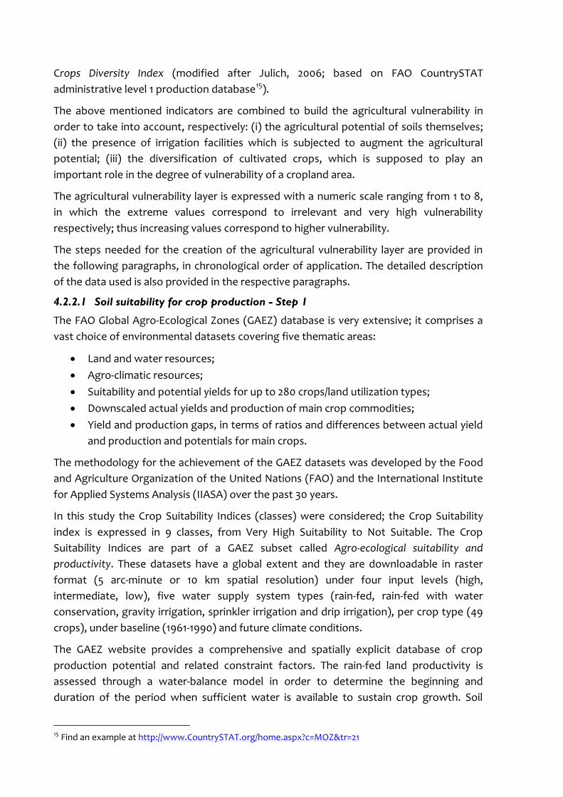
Crops Diversity Index (modified after Julich, 2006; based on FAO CountrySTAT
administrative level 1 production database14F
15).
The above mentioned indicators are combined to build the agricultural vulnerability in
order to take into account, respectively: (i) the agricultural potential of soils themselves;
(ii) the presence of irrigation facilities which is subjected to augment the agricultural
potential; (iii) the diversification of cultivated crops, which is supposed to play an
important role in the degree of vulnerability of a cropland area.
The agricultural vulnerability layer is expressed with a numeric scale ranging from 1 to 8,
in which the extreme values correspond to irrelevant and very high vulnerability
respectively; thus increasing values correspond to higher vulnerability.
The steps needed for the creation of the agricultural vulnerability layer are provided in
the following paragraphs, in chronological order of application. The detailed description
of the data used is also provided in the respective paragraphs.
4.2.2.1 Soil suitability for crop production - Step 1
The FAO Global Agro-Ecological Zones (GAEZ) database is very extensive; it comprises a
vast choice of environmental datasets covering five thematic areas:
Land and water resources;
Agro-climatic resources;
Suitability and potential yields for up to 280 crops/land utilization types;
Downscaled actual yields and production of main crop commodities;
Yield and production gaps, in terms of ratios and differences between actual yield
and production and potentials for main crops.
The methodology for the achievement of the GAEZ datasets was developed by the Food
and Agriculture Organization of the United Nations (FAO) and the International Institute
for Applied Systems Analysis (IIASA) over the past 30 years.
In this study the Crop Suitability Indices (classes) were considered; the Crop Suitability
index is expressed in 9 classes, from Very High Suitability to Not Suitable. The Crop
Suitability Indices are part of a GAEZ subset called Agro-ecological suitability and
productivity. These datasets have a global extent and they are downloadable in raster
format (5 arc-minute or 10 km spatial resolution) under four input levels (high,
intermediate, low), five water supply system types (rain-fed, rain-fed with water
conservation, gravity irrigation, sprinkler irrigation and drip irrigation), per crop type (49
crops), under baseline (1961-1990) and future climate conditions.
The GAEZ website provides a comprehensive and spatially explicit database of crop
production potential and related constraint factors. The rain-fed land productivity is
assessed through a water-balance model in order to determine the beginning and
duration of the period when sufficient water is available to sustain crop growth. Soil
15 Find an example at http://www.CountrySTAT.org/home.aspx?c=MOZ&tr=21
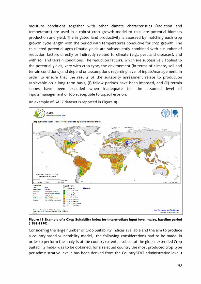
43
moisture conditions together with other climate characteristics (radiation and
temperature) are used in a robust crop growth model to calculate potential biomass
production and yield. The irrigated land productivity is assessed by matching each crop
growth cycle length with the period with temperatures conducive for crop growth. The
calculated potential agro-climatic yields are subsequently combined with a number of
reduction factors directly or indirectly related to climate (e.g., pest and diseases), and
with soil and terrain conditions. The reduction factors, which are successively applied to
the potential yields, vary with crop type, the environment (in terms of climate, soil and
terrain conditions) and depend on assumptions regarding level of inputs/management. In
order to ensure that the results of the suitability assessment relate to production
achievable on a long term basis, (i) fallow periods have been imposed, and (ii) terrain
slopes have been excluded when inadequate for the assumed level of
inputs/management or too susceptible to topsoil erosion.
An example of GAEZ dataset is reported in Figure 19.
Figure 19 Example of a Crop Suitability Index for intermediate input level maize, baseline period
(1961-1990).
Considering the large number of Crop Suitability Indices available and the aim to produce
a country-based vulnerability model, the following considerations had to be made: in
order to perform the analysis at the country extent, a subset of the global extended Crop
Suitability Index was to be obtained; for a selected country the most produced crop type
per administrative level 1 has been derived from the CountrySTAT administrative level 1

production database (expressed in weight and downloadable in table format 15F
16); the
corresponding Crop Suitability Index dataset has then been retrieved from the GAEZ
database (choosing by default an intermediate input level and the baseline climate
conditions).
The extraction of the most produced crop per administrative level 1 was performed
through a self-developed Matlab procedure (see Annex I - Matlab script for CDI).
CountrySTAT is a web-based information technology system for food and agriculture
statistics at the national and subnational levels. It centralizes and integrates the data
coming from various sources and allows to harmonize them according to international
standards. Depending on the countries considered, it gathers institutional statistical
information from population census to agricultural, fisheries and livestock production.
However, data aggregation level and availability vary considerably among countries.
Despite the efforts made at harmonizing data, information tables are often incompatible
country by country (see an example in Annex II - CountrySTAT raw data). This issue is
challenging if the data are to be used in automatic procedures, therefore a manual
preprocessing was needed to be performed in order to prepare the data for the analysis.
Eventually the different Crop Suitability indexes, one per each administrative level 1, were
mosaicked to obtain the whole country coverage. The final product of this phase is a map
showing the spatial distribution of the suitability of the terrain to produce a particular
type of crop, specifically the most produced crop on a historical basis (Figure 20).
Figure 20 For each admin level 1 (on the left) the main cultivated crop has been calculated over
the available time series. The corresponding crop suitability has been extracted from the GAEZ
database and the whole country was mapped by merging different administrative suitability tiles
(middle and right). Suitability increases from light green to dark red.
4.2.2.2 Global Map of Irrigation Areas - Step 2
The suitability class values obtained in step 1 (see 4.2.2.1) were revised by considering the
Global Map of Irrigation Areas (GMIA) dataset.
The latest version of the map shows the amount of area equipped for irrigation around
the year 2005 in percentage of the total pixel area on a raster with a resolution of 5 arc-
minute (10 km at the equator) (Siebert, Henrich, Karen, & Burke, 2013). Additional map
layers report the percentage of the area equipped for irrigation that was actually used for
16 Find an example at http://www.CountrySTAT.org/home.aspx?c=MOZ&tr=21

45
irrigation and the percentages of the area equipped for irrigation that was irrigated with
groundwater, surface water or non-conventional sources of water. The first global digital
map of irrigated areas, obtained on the basis of cartographic information and FAO
statistics, has a resolution of 0.5 degree and was developed in 1999 by the Center for
Environmental Systems Research of the University of Kassel. The latest version of the
map is reported in Figure 21.
Figure 21 Global Map of Irrigation Areas version 5.0, values are expressed in percentage of the
pixel occupied by irrigation systems.
The suitability layer, obtained in step 1, and the GMIA dataset were firstly superimposed.
Each suitability pixel value was then multiplied by 5% of the corresponding GMIA pixel
value, thus augmenting the suitability class when a considerable portion of the pixel area
is identified as equipped with irrigation systems. The result of this operation is reported in
Figure 22, which represents the suitability layer weighted with the percentage of
irrigation area per pixel.
4.2.2.3 Crop Diversity Index - Step 3
The Crop Diversity Index (CDI) can be considered as an indicator of the resilience of the
households living in the area over which is calculated, and should thus diminish the value
of the agricultural vulnerability.
The Crop Diversity Index was calculated as suggested in Julich, (2006) and modified by
Eriygama, Smakhtin, & Gamage, (2009) eventually reworked by the author as follows:
∑ [4]
where:
P is the administrative level 1 mean production, over the available time series, of each
type of crop divided by the sum of the mean total production.
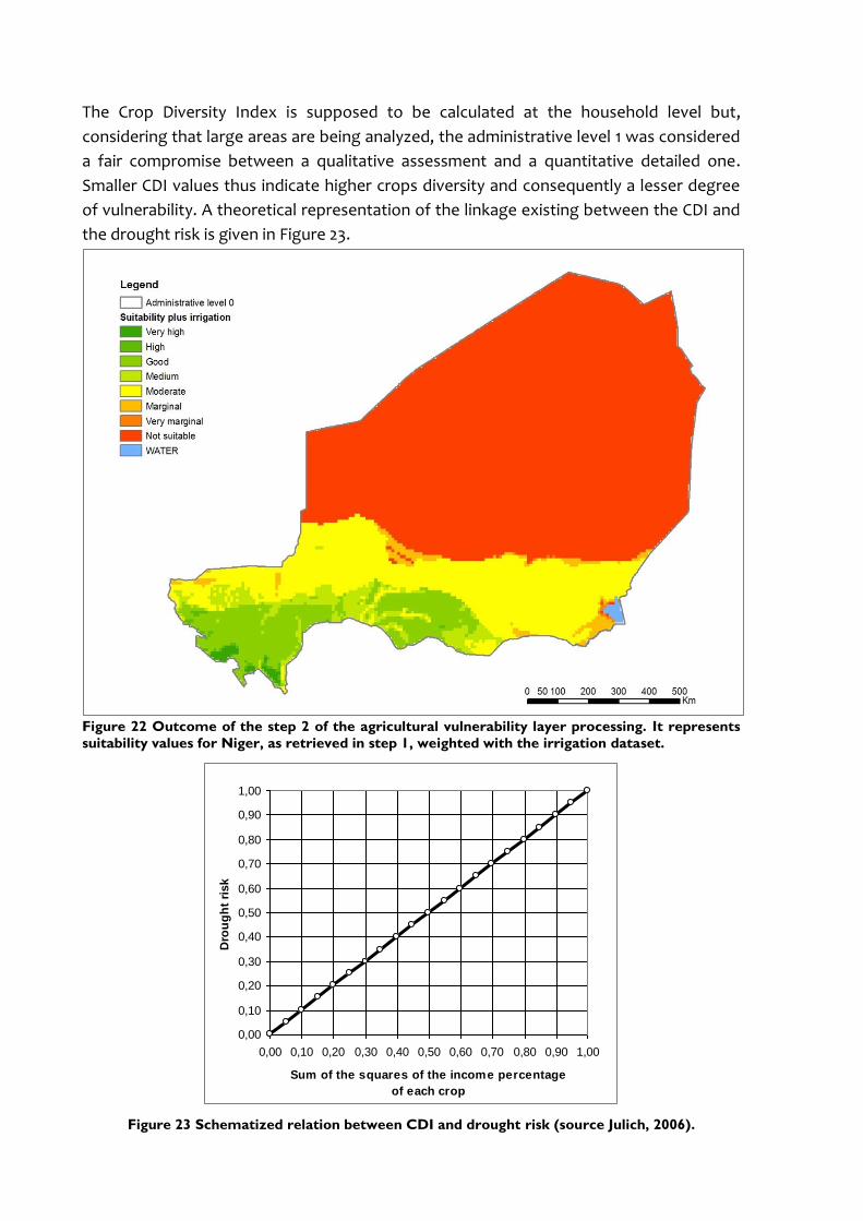
The Crop Diversity Index is supposed to be calculated at the household level but,
considering that large areas are being analyzed, the administrative level 1 was considered
a fair compromise between a qualitative assessment and a quantitative detailed one.
Smaller CDI values thus indicate higher crops diversity and consequently a lesser degree
of vulnerability. A theoretical representation of the linkage existing between the CDI and
the drought risk is given in Figure 23.
Figure 22 Outcome of the step 2 of the agricultural vulnerability layer processing. It represents
suitability values for Niger, as retrieved in step 1, weighted with the irrigation dataset.
Figure 23 Schematized relation between CDI and drought risk (source Julich, 2006).
0,00
0,10
0,20
0,30
0,40
0,50
0,60
0,70
0,80
0,90
1,00
0,00 0,10 0,20 0,30 0,40 0,50 0,60 0,70 0,80 0,90 1,00
Sum of the squares of the income percentage
of each crop
Dro
ug
ht
risk

47
Production data were retrieved from FAO CountrySTAT administrative level 1 production
database. The index was calculated for the whole set of countries available at FAO
CountrySTAT platform by means of a self-developed Matlab procedure (see Annex I -
Matlab script for CDI). The CDI values calculated per administrative level 1 were assigned
to their respective administrative boundaries (GAUL) in a polygon vector format.
The CDI layer was superimposed to the layer obtained in step 2 (see 4.2.2.2): the pixel of
the latter were augmented by a class of vulnerability where the CDI value was bigger than
0,5 unit, given the fact that the CDI is expressed in values that are inversely proportional
to the variety of cultivated crops.
Figure 24 Crop Diversity Index calculated for the Administrative boundaries level 1 of Niger,
represented here in polygon format.
4.2.3 Risk surface
Each risk monitoring system has its own unit to which the alert is attached. On the basis
of the procedure with which the hazard or the risk is monitored, the alert is then
calculated or aggregated according to specific units. In the present case it has been
decided to define specific risk units that are shaped on the basis of various assumptions
and models (e.g. poverty distribution and mapping). The objective was to create units
that represent people’s strategy to sell and buy staple foods. In this way the hazard that
hits a particular unit is departed on a homogeneous surface in which the potential
impacts could occur.
Three alternative risk surfaces were then created as follows. In the first case an
accessibility term was considered; this takes into account both physical distance and
travel times (see 4.2.3.1) to identified food source location (i.e. markets or settlements,
see 4.2.3.2). In the second case, a food source specific characteristic was used to model
the people attraction exerted by the different sources type considered (see 4.2.3.3). In

the third case, traditional market flows of goods were enclosed in the model to better
represent market catchments (see 4.2.3.3).
In the following paragraphs the models and assumptions applied in order to shape the
three types of risk surfaces are described in details.
4.2.3.1 Accessibility – Risk surface I
The term accessibility refers to the distance to a location of interest and the ease with
which this location can be reached (Goodall, 1987). In the presented vulnerability model
the factor that is here introduced, through the use of a risk surface calculated with an
accessibility model, has an environmental nature as well as a social one; in fact it has been
proven that better access to population and markets centers can lead to diversification of
rural economies and contribute positively to the wellbeing of populations. Despite the
fact that the important linkages between market access and poverty (e.g. food
availability and access) are well known, few studies have tried to pragmatically analyze
and model this relationship (F. Pozzi, Robinson, & Nelson, 2010).
The concept of accessibility is borrowed from poverty distribution studies to assume in
this work a value inferring the probability, for people living in a determined area, to be
able to displace for selling and buying commodities at a specific location.
The considered country was subdivided into market catchment areas calculated on the
basis of the easiness to access important markets or most populated cities. These
locations were identified through a market survey described in 4.2.3.2. The accessibility
was intended as a friction surface that takes into account distance and travel times to
markets. When building this type of risk surface the markets were considered equally
important. Travel times were calculated as suggested in Pozzi & Robinson, 2008 through
the following steps:
I. A speed value is assigned to each type of land cover (retrieved from ESA
GlobCover dataset, see Table 2) and each type of road (retrieved from VMAP0, see
Table 2) according to the categorization reported in Table 3.
II. Speed values are weighted with slope values (derived by an elevation dataset, i.e.
GLOBE DEM, see Table 2), previously categorized into classes of steepness (see
Table 4). At this stage a cost surface, in the form of a raster, is obtained. This cost
surface is expressed in time needed to cross each cell.
III. A cost allocation calculation, embedded as a system tool in ESRI ArcGis desktop
software, is performed; the tool determines, for each cell, the least cost path to
reach the nearest source location. A cost distance raster is then produced; each of
its cell contains the value, in minutes, needed to reach the identified nearest
source location. On the basis of this operation the tool gives also as output a cost
allocation raster in which to each cell is assigned the value of the source location
identified as the nearest. The country surface is so divided into areas belonging to
a specific market. The entire country surface is covered by this classification.
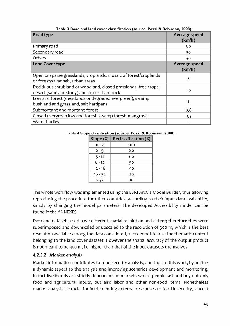
49
Table 3 Road and land cover classification (source: Pozzi & Robinson, 2008).
Road type Average speed (km/h)
Primary road 60
Secondary road 30
Others 30
Land Cover type Average speed (km/h)
Open or sparse grasslands, croplands, mosaic of forest/croplands or forest/savannah, urban areas
3
Deciduous shrubland or woodland, closed grasslands, tree crops, desert (sandy or stony) and dunes, bare rock
1,5
Lowland forest (deciduous or degraded evergreen), swamp bushland and grassland, salt hardpans
1
Submontane and montane forest 0,6
Closed evergreen lowland forest, swamp forest, mangrove 0,3
Water bodies -
Table 4 Slope classification (source: Pozzi & Robinson, 2008).
Slope (%) Reclassification (%)
0 - 2 100
2 - 5 80
5 - 8 60
8 - 12 50
12 - 16 40
16 - 32 20
> 32 10
The whole workflow was implemented using the ESRI ArcGis Model Builder, thus allowing
reproducing the procedure for other countries, according to their input data availability,
simply by changing the model parameters. The developed Accessibility model can be
found in the ANNEXES.
Data and datasets used have different spatial resolution and extent; therefore they were
superimposed and downscaled or upscaled to the resolution of 300 m, which is the best
resolution available among the data considered, in order not to lose the thematic content
belonging to the land cover dataset. However the spatial accuracy of the output product
is not meant to be 300 m, i.e. higher than that of the input datasets themselves.
4.2.3.2 Market analysis
Market information contributes to food security analysis, and thus to this work, by adding
a dynamic aspect to the analysis and improving scenarios development and monitoring.
In fact livelihoods are strictly dependent on markets where people sell and buy not only
food and agricultural inputs, but also labor and other non-food items. Nonetheless
market analysis is crucial for implementing external responses to food insecurity, since it

is recognized that market presence can alleviate or aggravate food insecurity (Beekhuis &
Laouali, 2007; Sanogo, n.d.).
The presence of markets makes an important contribution to the pillars of food security
(i.e. availability, access and use, for more details refer to section 2.5), and this is the
reason why it has been decided to include a market analysis in the vulnerability model
herein presented. The above-mentioned contributions are listed in the following (FAO,
2008):
Availability - producers are able to purchase food and inputs for producing food.
The movement of food through a country’s market network, from surplus to
deficit areas and across borders, may help to ensure stable food supplies over
time and space. Moreover countries can trade with each other to provide enough
food to satisfy population’s needs.
Access - households sell their products (e.g. crops, livestock, and non-agricultural
commodities) and their labor in the market to earn income. The price of food in
the market determines whether a household’s income or resources are sufficient
to purchase an adequate amount of quality food.
Moreover an efficient and adequate marketing system is a presumption for agricultural
diversification, which guarantees better prices to producers who sell their harvest and
the availability of competitively priced produce to consumers (Tracey-White, 1999). For
the sake of this work a market survey was conducted in order to properly choose
reference markets to include in the analysis. The aim was to identify typical market
categories that can be observed in developing countries.
The main broad classification that can be applied to markets refers to the context
considered (Tracey-White, 1999), i.e.:
rural context - primarily concerned with the infrastructure needs of producers for
the assembly and marketing of surplus produce to urban areas and export;
urban context - concerned with the wholesale and retail distribution of food
products to consumers within an urban area and with further distribution to other
urban areas and for export.
The linkage between rural and urban areas is normally provided by a network of market
intermediaries, such as the following list provided by Tracey-White, 1999:
farmers selling directly in the market (very common in rural markets);
petty traders and assemblers;
wholesalers;
commission agents, sometimes acting as auctioneers, and brokers;
transporters and transport agents;
retailers.
The agricultural market network normally includes the following types of market (Tracey-
White, 1999):
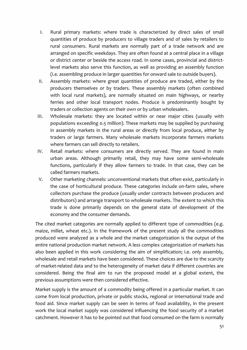
51
I. Rural primary markets: where trade is characterized by direct sales of small
quantities of produce by producers to village traders and of sales by retailers to
rural consumers. Rural markets are normally part of a trade network and are
arranged on specific weekdays. They are often found at a central place in a village
or district center or beside the access road. In some cases, provincial and district-
level markets also serve this function, as well as providing an assembly function
(i.e. assembling produce in larger quantities for onward sale to outside buyers).
II. Assembly markets: where great quantities of produce are traded, either by the
producers themselves or by traders. These assembly markets (often combined
with local rural markets), are normally situated on main highways, or nearby
ferries and other local transport nodes. Produce is predominantly bought by
traders or collection agents on their own or by urban wholesalers.
III. Wholesale markets: they are located within or near major cities (usually with
populations exceeding 0.5 million). These markets may be supplied by purchasing
in assembly markets in the rural areas or directly from local produce, either by
traders or large farmers. Many wholesale markets incorporate farmers markets
where farmers can sell directly to retailers.
IV. Retail markets: where consumers are directly served. They are found in main
urban areas. Although primarily retail, they may have some semi-wholesale
functions, particularly if they allow farmers to trade. In that case, they can be
called farmers markets.
V. Other marketing channels: unconventional markets that often exist, particularly in
the case of horticultural produce. These categories include on-farm sales, where
collectors purchase the produce (usually under contracts between producers and
distributors) and arrange transport to wholesale markets. The extent to which this
trade is done primarily depends on the general state of development of the
economy and the consumer demands.
The cited market categories are normally applied to different type of commodities (e.g.
maize, millet, wheat etc.). In the framework of the present study all the commodities
produced were analyzed as a whole and the market categorization is the output of the
entire national production market network. A less complex categorization of markets has
also been applied in this work considering the aim of simplification; i.e. only assembly,
wholesale and retail markets have been considered. These choices are due to the scarcity
of market-related data and to the heterogeneity of market data if different countries are
considered. Being the final aim to run the proposed model at a global extent, the
previous assumptions were then considered effective.
Market supply is the amount of a commodity being offered in a particular market. It can
come from local production, private or public stocks, regional or international trade and
food aid. Since market supply can be seen in terms of food availability, in the present
work the local market supply was considered influencing the food security of a market
catchment. However it has to be pointed out that food consumed on the farm is normally

not included in the market supply, in this work this term is considered negligible and only
the local supply is considered.
The localization of market centers has been retrieved, for the analyzed case studies, from
local surveys mainly conducted by international humanitarian organizations. These have
been used as is in the case of the accessibility model, while they have been given an
importance factor in the case of gravity models (see paragraph 4.2.3.3).
4.2.3.3 Gravity models – Risk surface II
Market areas own an economic sense that does not correspond to other more commonly
used territorial or administrative divisions (e.g. towns, provinces, regions or countries). In
this paragraph various theories of delineation of trade areas will be presented. These
concepts, while not conceived for the purpose of market analysis in developing countries,
are considered of interest for this application and promising in the field of market
catchment automatic delineation. In particular, the possibility of overlooking periodical
field survey data is extremely important in the context of monitoring and early warning
systems, especially when applied to developing countries.
Reilly (1931) was the first in tackling the delimitation market problem. Based on the
Newtonian law of gravitation, his model is the precursor of the gravity spatial choice
models commonly used today. Many studies have later implemented and sharpened his
statements, opening an important path in geographical marketing (Applebaum & Cohen,
1961; Christaller, 1933; Fotheringam & O’Kelly, 1989; Huff, 1962; Jones & Mock, 1984; Rust
& Donthu, 1995).
Reilly’s law of retail gravitation considers both distance and attractiveness of alternative
shopping opportunities. The notion that agglomeration tends to increase the
attractiveness of stores is key to Reilly’s law, i.e. stores located in centers with greater
populations draw customers from farther distances than those in less inhabited centers.
Based on the Newtonian law of gravitation, Reilly’s theory was the first to state that
consumers trade off the cost of travel with the attractiveness of alternate purchasing
opportunities. This deterministic law states that the proportion of retail trade attracted
from intermediate towns by two competing centers is directly proportional to their
population and inversely proportional to the square of the distances from those centers
to the intermediate towns. The attractiveness of a center is measured by means of two
variables: center population (i.e. the mass term), which exerts a positive attraction over
consumers, and distance (i.e. the friction term), which discourage consumers from
moving. The mass variable can be expressed as the size of the towns in terms of
population or as sales surface (e.g. square meters) (Chasco Yrigoyen & Vicéns Otero,
1998). However as Fotheringam and O’Kelly (1989) pointed out, the gravitation model is
based on the assumption that though the variables that explain the spatial choice of an
individual tend to be very similar to those that explain the spatial choices of a large
number of individuals, on the individual level, spatial choice is evidently more behavioral.

53
A step forward in the spatial choice model development was made in 1963 by Huff, who
was the first to propose a spatial-interaction model for estimating retail trade areas. His
theory takes into account the fact that when consumers have various shopping
opportunities, they would probably visit several different stores rather than restrict their
choice to a single outlet.
Figure 25 The spatial choice problem (source: Chasco Yrigoyen & Vicéns Otero, n.d.).
This assumption lead to the consequence that each store within the analyzed geographic
area has some chance of being patronized. Therefore Huff introduced a probabilistic
approach for the definition of trade areas, i.e. each store has a certain probability of being
chosen by consumers. This probability increases with a so called attractiveness factor of
the outlet and decreases with the square of the distance. Huff’s probability function is
provided in equation [5]:
∑
∑
[5]
where
i: is the location of the consumer;
Pij: probability of consumer at i visiting store j (or town j);
J: is the set of competing stores (or towns) in the region;
Uij: utility of store (or town) j for individual at i;
Sj : size of outlet j (or set of outlets of town j);
Dij: distance between consumer at i and store (or town) j;
α, β: sensibility parameters (α = 1 and β = -2).
Huff introduced in his formula [5] the concept of utility (U) of a store, which depends on
its size (S) and distance (D) from consumer location. To determine the probability of a
consumer visiting a particular store (Pij), Huff used Luce’s axiom (1959), which postulates
that this probability equals the ratio of the utility of the considered store (Uij) to the sum
of utilities of all the stores in the geographic area analyzed.
In order to adapt Huff’s law to the present study several considerations had to be made:
it is unlikely that people’s strategy to buy and sell commodities in developing
countries is submitted to the same assumptions made for retail trade area
definition (e.g. possibility to move across relatively long distances);

the mere size of markets, whether the data is available, is possibly a variable that
does not represent correctly their attractiveness for the consumers;
when a whole country surface has to be analyzed, the Euclidean distance may not
be a realistic way to measure distances.
The above-mentioned issues were addressed as follows:
the size of the store (S) was substituted with an importance factor related to the
type of market; i.e. markets were assigned importance values of 3, 2 or 1 when
belonging to the categories Wholesale, Assembly and Retail, respectively;
the Euclidean distance (D) was replaced by the distance calculated with the
accessibility model (see paragraph 4.2.3.1) in order to take into account physical
hindrances and therefore rather realistic travel times.
It should be noted that the use of different variables in place of the size of the store and
the use of a sort of weighted distances was previously suggested by other researchers
(Chasco Yrigoyen & Vicéns Otero, 1998).
To calculate the modified Huff gravity model a three step workflow has been
implemented in a GIS environment. The Model Builder, embedded in ESRI ArcGIS desktop
software, was used in order to be able to reproduce the workflow when needed (see the
ANNEXES for the Huff tool explanation).
In the first step the accessibility distance, expressed as travel times in minutes, is
calculated for the whole country surface for one market at a time. The accessibility
distance is multiplied for the importance factor, previously assigned to each market. A
number of utility raster equal to the number of markets is produced. In the second step,
the ratio of the utility per market to the sum of utilities is calculated per each market at a
time. The result of this process is a set of raster, each of that representing the probability
for a consumer to visit the market considered. Therefore each pixel of one of these
rasters own a value of probability related to a particular market, which depends not only
on the distance to and importance of that market but also on the utility of all the other
markets included in the analysis. The third step compares the probability rasters obtained
from the previous step and returns as outputs: (i) the maximum probability value for each
pixel and (ii) an identifier of the raster (i.e. a specific market) to which this maximum
value belongs.
A representation of the whole workflow applied to implement the Huff gravity model is
given in Figure 26.

55
Figure 26 Schematization of the building of risk surface implementing the gravity model. Dacc in
step 1 is the accessibility distance calculated for each cell i to reach market j or m. This value is
multiplied per the importance factor. The probability of a consumer to go to market j or m (Pi,j;
Pi,m) is calculated in step 2. Step 3 retrieves the highest probability for each cell and stores it in a
single raster.

4.2.3.4 Gravity models with market flows – Risk surface III
The risk surface of third type was built by using the gravity model output (see 4.2.3.3) and
by adding data related to known flow of staple food from a market to another. In fact it
has been proven that, especially in developing countries, traditionally production surplus
areas supply those areas that cannot satisfy their population food need with local
production, this happening even during average production years.
In order to consider these trades among markets, a good knowledge of the functioning
of the market network is needed. In the present work these information were retrieved
locally, thanks to WFP local offices, only in the case of Niger, therefore for this one and
only case the third risk surface was produced and experimented.
The practical case being exposed in section 4.3.1.2, only the main rationale behind the
procedure implemented to obtain the third risk surface is described here: by considering
the units of risk surface ii, and after the analysis of market flows, it has been decided to
distribute the alerts that relapse on traditionally food surplus areas over the areas that
are normally supplied by the latter. In the same way when food deficit areas are alerted,
the surplus areas where the food come from are screened and if none or minimal alert is
found, then the deficit area alert are diminished.
It must be pointed out that the risk surface iii is not spatially different from the second
one, whereas in the third one the relations among markets are taken into account in the
phase of alert spreading over risk surface units.
4.2.4 Weighted hazard
This paragraph explains the procedure implemented in order to produce the weighted
hazard per pixel. The output herein produced is an intermediate output functional to the
final alert. As reported in paragraph 4.2, the hazard produced by ITHACA vegetation
monitoring system has to be superimposed and weighted with the Agricultural
Vulnerability layer.
The considered hazard values (i.e. Seasonal Small Integral Percent Deviation) are
expressed in percentage of deviation with respect to the average value of the parameter
calculated over the whole time series, and can vary in the range +400 ÷ -400. Only the
negative values are considered in this study because they represent the anomalies that
can cause the drought impacts. On the other hand Agricultural vulnerability values are
expressed by classes of integer varying from 0 to 8, the ascending order accounting for
increasing vulnerability.
Firstly the hazard raster is clipped with the crop areas in order to consider only the alerts
that are meaningful because impacting a valuable land; then each retained hazard pixel is
multiplied by the agricultural vulnerability value. The resulting map is expressed in the
same units as the hazard; an example is given in Figure 27.
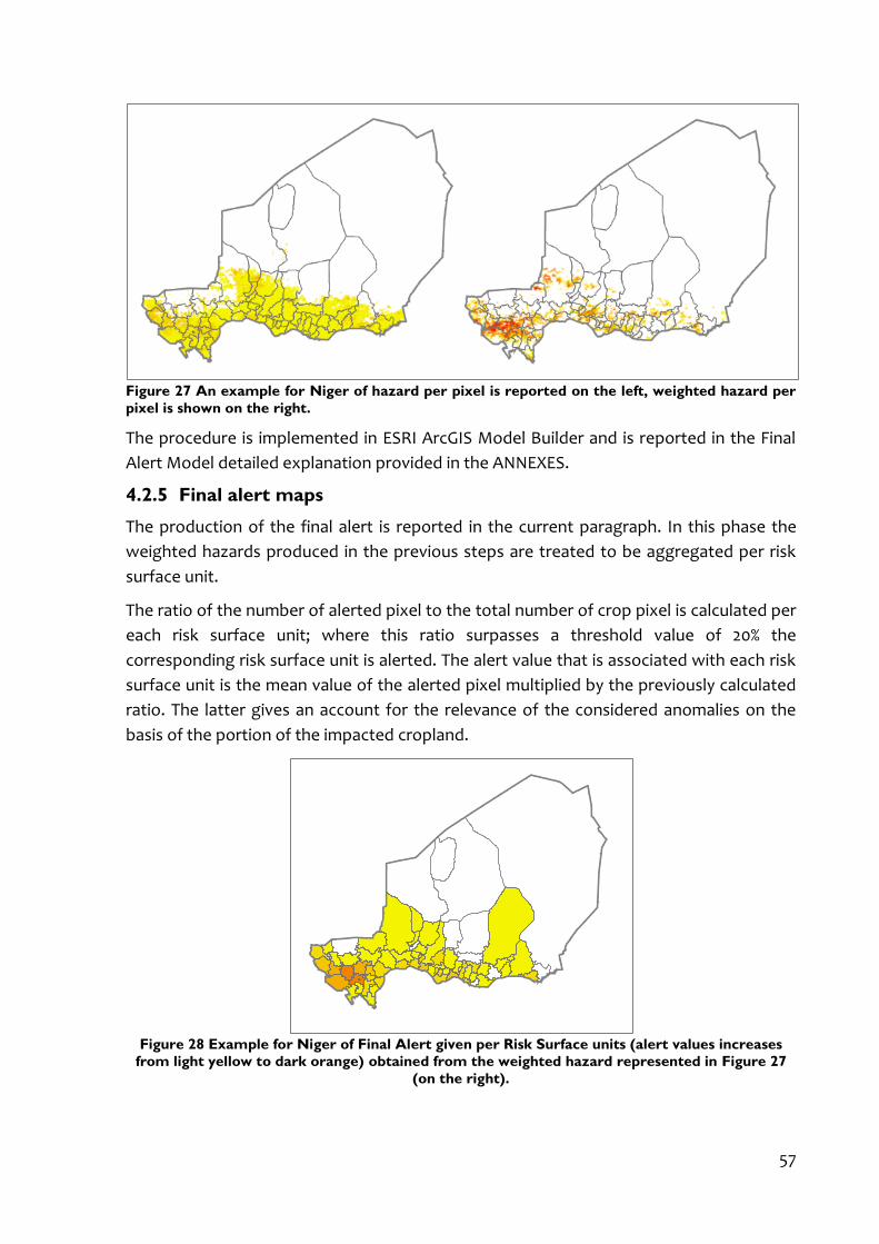
57
Figure 27 An example for Niger of hazard per pixel is reported on the left, weighted hazard per
pixel is shown on the right.
The procedure is implemented in ESRI ArcGIS Model Builder and is reported in the Final
Alert Model detailed explanation provided in the ANNEXES.
4.2.5 Final alert maps
The production of the final alert is reported in the current paragraph. In this phase the
weighted hazards produced in the previous steps are treated to be aggregated per risk
surface unit.
The ratio of the number of alerted pixel to the total number of crop pixel is calculated per
each risk surface unit; where this ratio surpasses a threshold value of 20% the
corresponding risk surface unit is alerted. The alert value that is associated with each risk
surface unit is the mean value of the alerted pixel multiplied by the previously calculated
ratio. The latter gives an account for the relevance of the considered anomalies on the
basis of the portion of the impacted cropland.
Figure 28 Example for Niger of Final Alert given per Risk Surface units (alert values increases
from light yellow to dark orange) obtained from the weighted hazard represented in Figure 27
(on the right).

This step of the procedure was implemented in ESRI ArcGIS Model Builder too, and is
reported in the Final Alert Model detailed explanation provided in ANNEXES. An example
of final alert aggregated per Risk Surface units is provided in Figure 28.
4.3 Case studies
The effectiveness of the inclusion of the proposed vulnerability model into the ITHACA
EWS was tested over a selection of country having experienced recurrent drought. The
vulnerability model was applied to the hazard, i.e. one of the products of the ITHACA
EWS, for the time series 2006-2013 thus generating one final alert per year and per
country. For each of the case studies the produced final alerts were compared with food
security historical data. One case study is located in Southern Africa (i.e. Mozambique)
and another one in Western Africa (i.e. Niger). Those two countries share with other
developing countries the issues of scarce data availability and difficult data remote access
when food security data are considered. Especially in those cases the usefulness of a EWS
for drought is undeniable, this was one of the reasons for those countries to be selected.
In particular for what concern Niger a field mission, performed during October 2013,
allowed to retrieve specific data linked to food security based on periodic field surveys
(see 4.4.2) that made possible the development of a quantitative evaluation of the final
alert produced.
An accounts of the characteristics of the two case studies, along with intermediate
outputs of model application, is provided in the following paragraphs.
4.3.1 Niger
Niger is a landlocked country located in the Sahara–Sahel belt. The Country is least-
developed, low-income, food-deficit and ranks last on the 2013 Human Development. It
has a population of over 16 million: life expectancy at birth is 55 years, the fertility rate is
among the highest in the world (7.6 births per woman) and the maternal mortality ratio is
590 per 100,000 births. 16F
17
Only the half of Niger total area (over 1 million km2) is habitable due to adverse climatic
and soil conditions. Niger has a mainly dry climate with considerable temperature
variations. Yearly potential evaporation is 2 to 4 m, while rainfall reaches 800 mm and
falls to below 100 mm over almost half of the country. The rainfall pattern is Saharan in
the north where it practically never rains, and Sudano Sahelian in the south, where an
average of 600 mm of rain falls during approximately four months (from June to
September). Rainfall varies, however, from one region to another and its distribution is
very erratic (Geesing & Djibo, 2006). Temperatures can exceed 40 degrees Celsius during
the dry season, from March to June, while from November to February, they drop
considerably (Bernus, Hamidou, & Laclavère, 1980).
A very small percentage of the country is arable (Figure 29). Agriculture is practiced
mainly in the south, where millet and sorghum are traditionally grown but maize, sugar
17http://www.wfp.org/countries/niger/overview

59
cane and sweet potato can also be found. Vegetables and fruit trees are growing in the
depression of ancient rivers whereas rice is cultivated mainly along the Niger river
(Geesing & Djibo, 2006). Although livestock keeping is mainly limited to the northern
Niger, the share of cultivated land competes increasingly with breeding (Figure 30). In
Sahelian countries in general, land and water resources are subjected to an overwhelming
pressure due to population growth and a considerable decrease in rainfall rates (Collinet
& Valentin, 1984; Roose, 1977). In particular in Niger clearing and wood-exploitation
reduces significantly the original vegetation: just for the capital city Niamey, more than
11,000 tons of firewood are needed per year (Geesing & Djibo, 2006).
The economy of Niger is mainly funded on subsistence farming and stock-rearing, that
contributes 40% to the total GDP. Moreover the vast majority of the labour force is
employed in the agriculture and livestock breeding sectors. The agricultural yearly
production is around 3 million tons of cereals. Cowpeas, cotton and groundnuts are
mainly cultivated for export. Millet, sorghum, cassava, pulses, rice, sugar cane and
vegetables are grown for local consumption. Fishing is conducted in Lake Chad and in the
Niger river, and the catch is consumed or exported locally. Industry is very limited even
though Niger subsoil is very rich in important minerals (e.g. tin, gold, uranium) (Geesing &
Djibo, 2006).
Figure 29 Niger land cover (source: ESAGlobCover, 300 m resolution, © ESA 2010 and
UCLouvain, © ESA / ESA GlobCover Project).
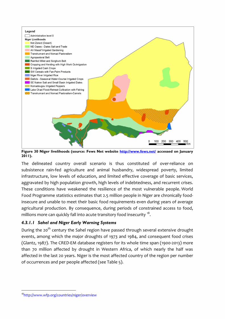
Figure 30 Niger livelihoods (source: Fews Net website http://www.fews.net/ accessed on January
2011).
The delineated country overall scenario is thus constituted of over-reliance on
subsistence rain-fed agriculture and animal husbandry, widespread poverty, limited
infrastructure, low levels of education, and limited effective coverage of basic services,
aggravated by high population growth, high levels of indebtedness, and recurrent crises.
These conditions have weakened the resilience of the most vulnerable people. World
Food Programme statistics estimates that 2.5 million people in Niger are chronically food-
insecure and unable to meet their basic food requirements even during years of average
agricultural production. By consequence, during periods of constrained access to food,
millions more can quickly fall into acute transitory food insecurity 17F
18.
4.3.1.1 Sahel and Niger Early Warning Systems
During the 20th century the Sahel region have passed through several extensive drought
events, among which the major droughts of 1973 and 1984, and consequent food crises
(Glantz, 1987). The CRED-EM database registers for its whole time span (1900-2013) more
than 70 million affected by drought in Western Africa, of which nearly the half was
affected in the last 20 years. Niger is the most affected country of the region per number
of occurrences and per people affected (see Table 5).
18http://www.wfp.org/countries/niger/overview
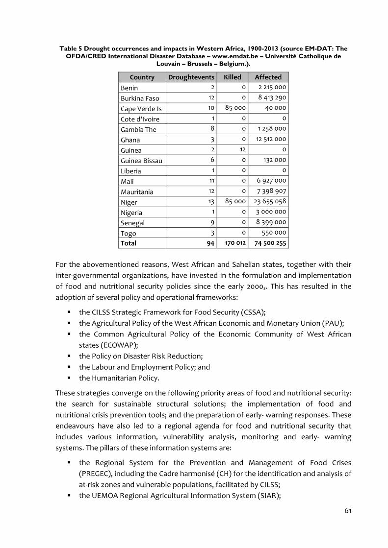
61
Table 5 Drought occurrences and impacts in Western Africa, 1900-2013 (source EM-DAT: The
OFDA/CRED International Disaster Database – www.emdat.be – Université Catholique de
Louvain – Brussels – Belgium.).
Country Droughtevents Killed Affected
Benin 2 0 2 215 000
Burkina Faso 12 0 8 413 290
Cape Verde Is 10 85 000 40 000
Cote d'Ivoire 1 0 0
Gambia The 8 0 1 258 000
Ghana 3 0 12 512 000
Guinea 2 12 0
Guinea Bissau 6 0 132 000
Liberia 1 0 0
Mali 11 0 6 927 000
Mauritania 12 0 7 398 907
Niger 13 85 000 23 655 058
Nigeria 1 0 3 000 000
Senegal 9 0 8 399 000
Togo 3 0 550 000
Total 94 170 012 74 500 255
For the abovementioned reasons, West African and Sahelian states, together with their
inter-governmental organizations, have invested in the formulation and implementation
of food and nutritional security policies since the early 2000s. This has resulted in the
adoption of several policy and operational frameworks:
the CILSS Strategic Framework for Food Security (CSSA);
the Agricultural Policy of the West African Economic and Monetary Union (PAU);
the Common Agricultural Policy of the Economic Community of West African
states (ECOWAP);
the Policy on Disaster Risk Reduction;
the Labour and Employment Policy; and
the Humanitarian Policy.
These strategies converge on the following priority areas of food and nutritional security:
the search for sustainable structural solutions; the implementation of food and
nutritional crisis prevention tools; and the preparation of early- warning responses. These
endeavours have also led to a regional agenda for food and nutritional security that
includes various information, vulnerability analysis, monitoring and early- warning
systems. The pillars of these information systems are:
the Regional System for the Prevention and Management of Food Crises
(PREGEC), including the Cadre harmonisé (CH) for the identification and analysis of
at-risk zones and vulnerable populations, facilitated by CILSS;
the UEMOA Regional Agricultural Information System (SIAR);

the ECOWAS Agricultural Information System (ECOAGRIS), serving as the
umbrella-platform for existing agricultural information systems;
the Observatory of agro-forestry- pastoral farms as well as the early- warning
mechanisms of producers’ organizations (POs), led by the West African Network
of Farmers’ and Agricultural Producers’ Organisations (ROPPA), the Billital
Maroobe Network (RBM) and the Association for the Promotion of Livestock in
the Sahel and Savannah (APESS).
The regional agenda counts also the Charter for Food Crisis Prevention and Management,
an assessment tool aimed at improving the effectiveness of food and nutritional
strategies and policies. Among the advisory and decision-making governance bodies and
networks the Food Crisis Prevention Network (RPCA) has to be cited for its preeminent
role in the Sahel region (SWAC/OECD, 2013).
At the same time country governments of the region themselves have developed
national early warning systems, integrated to different extents with regional systems.
The government of Niger, in particular, started to develop in 1989 an ensemble of early
warning tools constituting, as a whole, the national system for prevention and
management of disasters and food crises (Dispositif National de Prévention et de Gestion
des catastrophes et Crises Alimentaires, DNPGCCA). An overview of system components
and its connections is given in Figure 31. This apparatus counts a general secretariat
(Sécretariat Permanent, SP), that is a mechanism of consultation and fund mobilization,
an Information System, an Early Warning System (Système d’Alerte Précoce, SAP) and an
operational agency (Cellule Crises Alimentaires, CCA) (Cabinet du Premier Ministre du
Niger - DNPGCCA, 2013).
Moreover a coordination unit of the Early Warning System (Cellule de Coordination du
Système d’Alerte Précoce, CC/SAP) is in charge of the food security data gathering. This
unit relies on the following specific data collecting and analysis units:
Information system of the agricultural market (Système d’Information sur les
Marchés Agricoles, SIMA);
Information system of the pastoral market (Système d’Information sur les
Marchés à bétail, SIMb);
Harvest forecasting and estimation (Enquête Prévision et Estimation des Récoltes,
EPER);
Multidisciplinary working group (groupe de travail interdisciplinaire, GTI);
Specific working groups (groups sectoriels, GTP);
Regional and sub-regional committees in charge of the prevention and
management of food crises (Comités régionaux et sous-régionaux chargés de la
prévention et de la gestion des crises alimentaires, CR/PGCA et CSR/PGCA).
At the administrative level 3 (i.e. municipalities) a vulnerability observatory (Observatoire
du Suivi de la Vulnerabilité) coordinates the community-based monitoring system
(Système Communautaire d’Alerte Précoce et de Réponse aux Urgences, SCAP-RU).
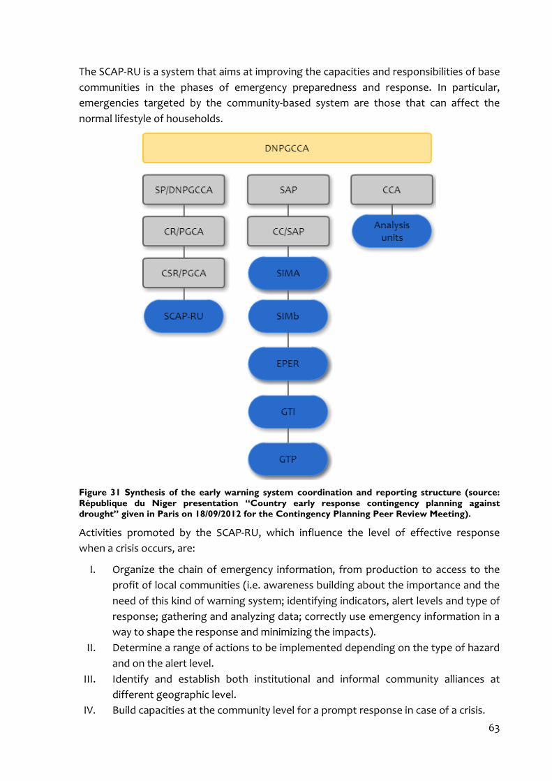
63
The SCAP-RU is a system that aims at improving the capacities and responsibilities of base
communities in the phases of emergency preparedness and response. In particular,
emergencies targeted by the community-based system are those that can affect the
normal lifestyle of households.
Figure 31 Synthesis of the early warning system coordination and reporting structure (source:
République du Niger presentation “Country early response contingency planning against
drought” given in Paris on 18/09/2012 for the Contingency Planning Peer Review Meeting).
Activities promoted by the SCAP-RU, which influence the level of effective response
when a crisis occurs, are:
I. Organize the chain of emergency information, from production to access to the
profit of local communities (i.e. awareness building about the importance and the
need of this kind of warning system; identifying indicators, alert levels and type of
response; gathering and analyzing data; correctly use emergency information in a
way to shape the response and minimizing the impacts).
II. Determine a range of actions to be implemented depending on the type of hazard
and on the alert level.
III. Identify and establish both institutional and informal community alliances at
different geographic level.
IV. Build capacities at the community level for a prompt response in case of a crisis.

V. Create and maintain a confidence level between the institutional warning system
(DNPGCCA) and the community one.
The complex Niger EWS, illustrated so far, is relatively new and continuously improved
year after year. In the actual situation zones in which the tasks of the respective
institutions are overlapped can be noticed, and a general lack of coordination of the
information chain as well. Nonetheless various UN programs and projects, as well as
international NGOs, developed their own monitoring and EW Systems that in some cases
still coexist with the governmental ones and in other cases contribute to it. As a result
various operative agencies are still using their own produced data, thus engendering
duplicate efforts and possibly controversial outputs.
In the described context it could be crucial to automatically and univocally determine: (i)
hazard levels that trigger drought crisis, (ii) spatial links between zones impacted by the
hazard and zones impacted by the effects. Tracking success and fails of existing EWS
would also be of help for better calibrating the systems. A transparent and effective
methodology would be helpful for operative agencies and their donors.
The proposed vulnerability model is run with available Niger data and, after being applied
to ITHACA EWS product, is validated with locally retrieved validation data (see 4.4.2) and
with regional food security outlooks produced by Fews Net (see 4.4.1).
4.3.1.2 Applied model, input and intermediate results
The conceptual model described in 4.2 was adapted to Niger case study; details are given
in the following.
Firstly the agricultural vulnerability surface was obtained as reported in 4.2.2. In order to
do so the most produced crops per administrative level 1 (given in Figure 32) were
retrieved from the FAO CountryStat database (local statistics). The Crop Diversity Index
was calculated using the same base data. The results are summarized in Table 6.
Table 6 Most produced crops and CDI given per Administrative level 1 of Niger.
Administrative level 1 Main Crop CDI
AGADEZ MAIZE 0,34
DIFFA MILLET 0,61
DOSSO MILLET 0,49
MARADI MILLET 0,34
TAHOUA MILLET 0,42
TILLABERI MILLET 0,56
ZINDER MILLET 0,33
NIAMEY (municipality) MILLET 0,45
The most produced crop for all regions, except Agadez, is millet as could be expected. In
fact this corn is widely consumed as staple food in Niger partly due to the fact that it is
adapted to its semi-arid climate. The phenomenon is also explicable considering that
farmers largely produce for their own consumption.
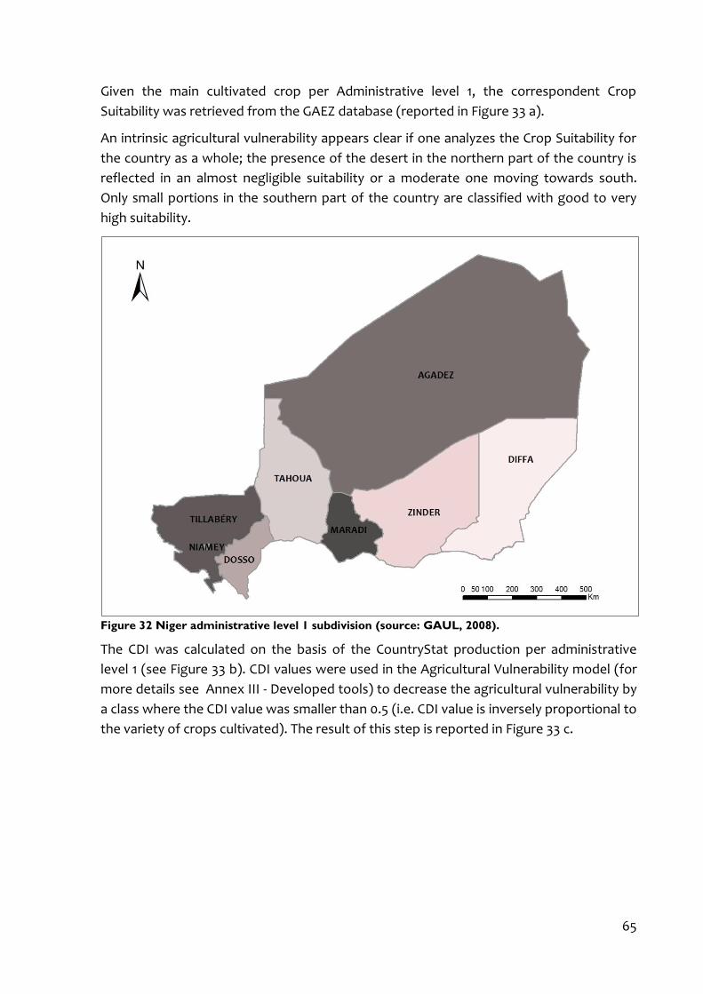
65
Given the main cultivated crop per Administrative level 1, the correspondent Crop
Suitability was retrieved from the GAEZ database (reported in Figure 33 a).
An intrinsic agricultural vulnerability appears clear if one analyzes the Crop Suitability for
the country as a whole; the presence of the desert in the northern part of the country is
reflected in an almost negligible suitability or a moderate one moving towards south.
Only small portions in the southern part of the country are classified with good to very
high suitability.
Figure 32 Niger administrative level 1 subdivision (source: GAUL, 2008).
The CDI was calculated on the basis of the CountryStat production per administrative
level 1 (see Figure 33 b). CDI values were used in the Agricultural Vulnerability model (for
more details see Annex III - Developed tools) to decrease the agricultural vulnerability by
a class where the CDI value was smaller than 0.5 (i.e. CDI value is inversely proportional to
the variety of crops cultivated). The result of this step is reported in Figure 33 c.
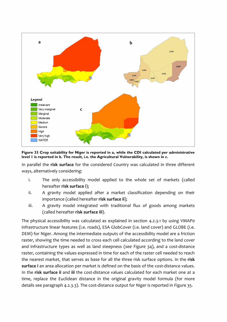
Figure 33 Crop suitability for Niger is reported in a, while the CDI calculated per administrative
level 1 is reported in b. The result, i.e. the Agricultural Vulnerability, is shown in c.
In parallel the risk surface for the considered Country was calculated in three different
ways, alternatively considering:
i. The only accessibility model applied to the whole set of markets (called
hereafter risk surface i);
ii. A gravity model applied after a market classification depending on their
importance (called hereafter risk surface ii);
iii. A gravity model integrated with traditional flux of goods among markets
(called hereafter risk surface iii).
The physical accessibility was calculated as explained in section 4.2.3.1 by using VMAP0
infrastructure linear features (i.e. roads), ESA GlobCover (i.e. land cover) and GLOBE (i.e.
DEM) for Niger. Among the intermediate outputs of the accessibility model are a friction
raster, showing the time needed to cross each cell calculated according to the land cover
and infrastructure types as well as land steepness (see Figure 34), and a cost-distance
raster, containing the values expressed in time for each of the raster cell needed to reach
the nearest market, that serves as base for all the three risk surface options. In the risk
surface i an area allocation per market is defined on the basis of the cost-distance values.
In the risk surface ii and iii the cost-distance values calculated for each market one at a
time, replace the Euclidean distance in the original gravity model formula (for more
details see paragraph 4.2.3.3). The cost-distance output for Niger is reported in Figure 35.
c
a b
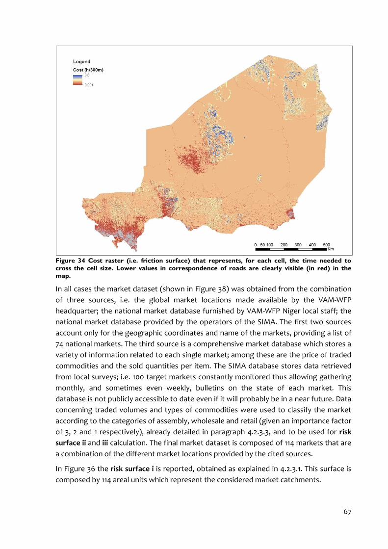
67
Figure 34 Cost raster (i.e. friction surface) that represents, for each cell, the time needed to
cross the cell size. Lower values in correspondence of roads are clearly visible (in red) in the
map.
In all cases the market dataset (shown in Figure 38) was obtained from the combination
of three sources, i.e. the global market locations made available by the VAM-WFP
headquarter; the national market database furnished by VAM-WFP Niger local staff; the
national market database provided by the operators of the SIMA. The first two sources
account only for the geographic coordinates and name of the markets, providing a list of
74 national markets. The third source is a comprehensive market database which stores a
variety of information related to each single market; among these are the price of traded
commodities and the sold quantities per item. The SIMA database stores data retrieved
from local surveys; i.e. 100 target markets constantly monitored thus allowing gathering
monthly, and sometimes even weekly, bulletins on the state of each market. This
database is not publicly accessible to date even if it will probably be in a near future. Data
concerning traded volumes and types of commodities were used to classify the market
according to the categories of assembly, wholesale and retail (given an importance factor
of 3, 2 and 1 respectively), already detailed in paragraph 4.2.3.3, and to be used for risk
surface ii and iii calculation. The final market dataset is composed of 114 markets that are
a combination of the different market locations provided by the cited sources.
In Figure 36 the risk surface i is reported, obtained as explained in 4.2.3.1. This surface is
composed by 114 areal units which represent the considered market catchments.
Figure 35 Cost distance calculated for 114 markets. Values are expressed in minutes needed to
reach the nearest market along the shortest cost-distance path.
These surfaces are uniquely dependent on the physical accessibility of markets. Each
surface unit is built by considering territorial continuity, presence of infrastructure and
type of land cover. Noticeably, in high density market zones these surface units are
limited in area by the presence of proximity markets. It should also be noted how risk
surface units (i.e. 114 units as the number of considered markets) differ from the
administrative level subdivisions (i.e. 36 subdivisions) that are subjected to different
spatial criteria.
The risk surface ii for Niger, along with the market locations symbolized according to
their importance, are reported in Figure 37. This surface is obtained, as detailed in section
4.2.3.3, by applying a spatial choice model based on Huff (1962) gravity spatial choice
theory.

69
Figure 36 Risk surface i, calculated on the basis of the accessibility to Niger main markets.
Figure 37 Risk surface ii calculated with the Huff gravity model for Niger main markets. Markets
are represented according to their classification (3, 2 and 1 assigned to assembly, wholesale and
retail markets respectively).
Local experts state that Niger markets are highly interconnected, in fact the Southern
regions of the country are historically the most productive ones creating, during average
production years, a surplus of staple food that is commercialized in Northern, traditionally
deficit, regions. Moreover, foreign markets of bordering countries such as Burkina Faso,
Benin, Nigeria and Chad furnish Niger markets with their products. In particular some of
the biggest markets of the southern part of Niger are supplied by foreign merchandise;
those in turn supply northern markets. Clearly, those kinds of trades vary year after year
being influenced by agricultural production levels of single countries of the whole African
region as well as by international price and market trends, thus their representation is
beyond the scope of this work. However, the importance for food security of this
transnational food trade is recognized by humanitarians; an attempt of capturing these
transactions is made by USGS and Fews Net which provide country market flow maps for
staple goods (see an example for Niger in Figure 40).
In the framework of the present study it has been decided to model only the Niger inner
market flows by using the information included in the SIMA market database. The risk
surface iii was obtained by considering the relations existing among markets, which are
reported in Table 7. It was decided to consider that the staple food market trades impact
as for 30% of the weighted hazard (details in section 4.2.3.4) calculated for a particular
market catchment: that is the weighted hazard calculated for markets that supply other
inner Niger markets is distributed, as the 30% of its value, among the market catchments
that are supplied. In an analogous way when a supplier market reports no detected
weighted hazard, the correspondent supplied market sees their weighted hazard
diminished by a 30% of their values.
The linkages among markets, reported in Table 7, are then represented in Figure 39.
Table 7 Niger market flow.
Market Is supplied by Supplies
ABALA MOULELA
Niamey
AYOROU GOUNGOU
TAMASKE Keita
Tanout
TCHADOUA Aguie
TCHINTABARADEN
TCHINTABORAK
TCHIROZERINE
TERA
TESSAOUA
TILLABERI
TORODI
BADAGUICHIRI Illela
Toudoun Aggua
TOUMOUR Diffa
TOUNFAFI LADAMA
71
Market Is supplied by Supplies
TSERNAOUA Birni n'konni
ZINDER COMMUNE Mirriah
BAKIN BIRJI
BALLEYARA
BAMBAYE Tahoua
BANKILARE
BARWA Diffa
BELLA ZENO
BILMA
BIRNI N'GAOURE
ABALAK Sabon Machi, Birni N'konni Abardak, Agadez, Arlit, Bilma, Dabaga, Tabelot, Tchintaborak, Tchirozerine
BIRNI N'KONNI
BOSSO
BOULAMARI Mainé-soroa
BOUREIMI Dogondoutchi
BOUTTI I Goudoumaria
BOUZA
DABAGA I
DAKORO
DAN SAGA (VA) Aguie
DANFAN Tahoua
ABARDAK (VA)
DEBI Aguie
DIFFA
DIOUNDIOU Gaya
DJADJI GANARAM Goudoumaria
Dogo
DOGONDOUTCHI
DOSSO
DOUNGASS
FALWEL
FAMALE (VA)
Niamey
AFFALA Tahoua
FILINGUE
FOURDIA
Gada
Gadira Bosso
GAGAMARI Diffa
GALMI
GANGARA Gazaoua
GAYA
GAZAOUA
GOTHEYE
Niamey

Market Is supplied by Supplies
AGADEZ
GOUDOUMARIA
Gouloudji
GOURE (CLA)
GUIDAN-ROUMJI Maradi
GUIDAN IDER
GUILLEY Tahoua
hamdallahi
IBOHAMANE Keita
ILLELA Badaguichiri
KABELAWA N'guigmi
AGUIE
KAOU (VA)
Kassama
Kazoé
keguel Maradi
KEITA Ibohamane
KILAKAM
KINJA HINDI
KIRTACHI
Niamey
KOLLO
Niamey
KORE MAIROUA
AMATALTAL
KOURIA
KOUTOUFANI Dosso
KOYGOROU Dosso
Léléwa N'guigmi
Liboré
LOGA
MADAOUA
MADAROUNFA
Madetta Bouza
MAGARIA
ARLIT
MAIJIRGUI Tessaoua
MAINE SOROA
MALLAM KOUARA
MARADI
MATAMEY
MAYAHI
Miriah
MOKKO Dosso
N'GUEL KOLO Diffa
N'GUIGMI
AYAWANE Bouza

73
Market Is supplied by Supplies
NIAMEY I
OUALLAM
ROGOGO Aguie
SABON KAFI Tanout
SABON MACHI Guidan Roumji
SAY
TABALAK Tahoua
TABELOT
TABOTAKI Bouza
TAHOUA I

Figure 38 Niger markets.
75
Figure 39 Risk surface calculated with the Huff gravity model for Niger main markets and then
linked according to inner market flows. Highlighted in light green and light orange are the two
main existing flows of food. Marketplaces are represented according to their classification.
Figure 40 Production and market flow map for Niger millet produced by USGS and other Fews
Net partners.

4.3.2 Mozambique
Mozambique is a country in the southeastern Africa, bordered by the Mozambique
Channel (India Ocean) and located between South Africa and Tanzania.
According to 2013 estimates, it has a population of over 24 million, with a life expectancy
of only 48 years. Aside from Niger and Democratic Republic of the Congo, the country
ranks at the bottom of the 2012 Human Development Index, at 185th position out of 187
countries19. Moreover, with one third of the population and 43 percent of the children
under five malnourished, Mozambique is dramatically food-deficit20.
After the independence gained in 1975 from the Portuguese succeeding four centuries of
colonialism, Mozambique fell in a long and destructive civil war lasted 16 years and ended
in 1992. Since the end of the 1980s, the governments launched a series of macroeconomic
and financial reforms designed to stabilize the economy. These steps, combined with
donor assistance and with two decades of peace and stability, have led to outstanding
improvements in the country growth rate (one of Africa's best performances). Due to its
booming extractive industry and inflows of large investments (40% of its 2012 annual
budget consist in foreign assistance), Mozambique has achieved a real GDP of 7.4 percent
in 201221 22.
Nevertheless, agriculture continues to be the pillar of the economy: the vast majority of
the Mozambique workforce is employed in this sector, more than 80 percent,
contributing to the 29.9% of the GDP in 201223. It is essentially a subsistence agriculture
conducted by smallholder farmers, which accounts for the 95% of the country agricultural
production24. Nowadays the potential agricultural development is high, in fact only about
10 percent of the arable land is estimated to be cultivated (circa 5 million of hectares)
(FAO, 2013).
Mozambique is characterized by a variety of agro-climatic zones ranging from arid and
semi-arid areas, in the south and south-west, to sub-humid zones or humid highlands in
the central and Northern provinces. Therefore, the southern zones with poor soil
conditions and scarce rainfalls are the most vulnerable and are subject to recurrent
droughts. Conversely, the northern and central areas are the most fertile with a high
agro-ecological potential; generally, these provinces are already producing agricultural
surpluses.
Tree crops such as coconut and cashew, particularly cultivated in the populated littorals
of Inhambane and Gaza, are an important source of foreign exchange earnings. Other
important productions include cotton (between 150,000 and 180,000 hectares), tobacco,
oilseeds, tea, citrus and horticultural crops, particularly tomatoes. Most of the irrigated
19 http://hdr.undp.org/en/countries 20 http://www.wfp.org/countries/mozambique/overview 21 https://www.cia.gov/library/publications/the-world-factbook/geos/mz.html 22 http://www.wfp.org/countries/mozambique/overview 23 https://www.cia.gov/library/publications/the-world-factbook/geos/mz.html 24 http://coin.fao.org/cms/world/mozambique/en/Home.html

77
areas (about 35,000 of 55,000 total hectares) are instead used by industrial plantations of
sugarcane. With an overall 40,000 hectares, this cultivation has increased rapidly over the
last decade reaching approximately 3 million tons by 2010. Major staples cultivated in
Mozambique are maize and cassava followed by sorghum, beans, groundnuts, millet and
rice. The seasonal calendar is characterized by two main growing seasons in the southern
part of the country, while one season is found in the northern part (see Figure 42).
Concerning breeding, cattle, goats and sheep are the principal livestock reared in
extensive grass-based systems, whereas pigs and poultry are kept mainly at household
level25.
Figure 41 Mozambique land cover (source: ESA GlobCover, 300 m resolution, ©ESA 2010 and
UCLouvain, ©ESA/ESA GlobCover Project).
Potentially, Mozambique could become not only a self-sufficient country in food
production but even a regional exporter26. However, the agricultural systems are
predominantly rain-fed, therefore the production can fluctuate widely from year to year27.
Considering that the country is recurrently shocked by intensive climatic events (i.e.
droughts, floods and cyclones) income from farming is often compromised contributing
to food insecurity, while also causing loss of life, ruining livelihoods and damaging
infrastructures. In this scenario, among African countries, Mozambique is the third most
25 http://www.fao.org/docrep/012/ak350e/ak350e00.htm 26 http://coin.fao.org/cms/world/mozambique/en/Home.html 27 http://www.fao.org/docrep/012/ak350e/ak350e00.htm

affected by weather-related hazards. In average, floods occur every two to three years
along the major river basins and more than 60 percent of the population lives in coastal
areas which are vulnerable to rapid on-set disasters28.
Figure 42 Mozambique seasonal calendar for a typical year (source: FEWS NET, retrieved from
http://www.fews.net/southern-africa/mozambique accessed on 20/02/2014).
4.3.2.1 Applied model, input and intermediate results
As done for the case of Niger the most produced crop and the Crop Diversity Index were
calculated on the basis of the FAO CountryStat database at the first level administrative
boundaries. The results are reported in Table 8.
Table 8 Most produced crops and CDI given per Administrative level 1 of Mozambique.
Administrative level 1 Main Crop CDI
NIASSA CASSAVA 0,29
CABO DELGADO CASSAVA 0,46
NAMPULA CASSAVA 0,66
ZAMBEZIA CASSAVA 0,63
TETE MILLET 0,29
MANICA MILLET 0,29
SOFALA CASSAVA 0,25
INHAMBANE CASSAVA 0,78
GAZA CASSAVA 0,34
MAPUTO CASSAVA 0,36
The CDI was used, as explained in 4.2.2, to weigh the Crop suitability index retrieved from
GAEZ specifically for each of the most produced crop of Mozambique regions. The result
of the process, after being weighted with the GMIA dataset too, is the agricultural
vulnerability layer of Mozambique, which is provided in Figure 44.
28 http://www.wfp.org/countries/mozambique/overview
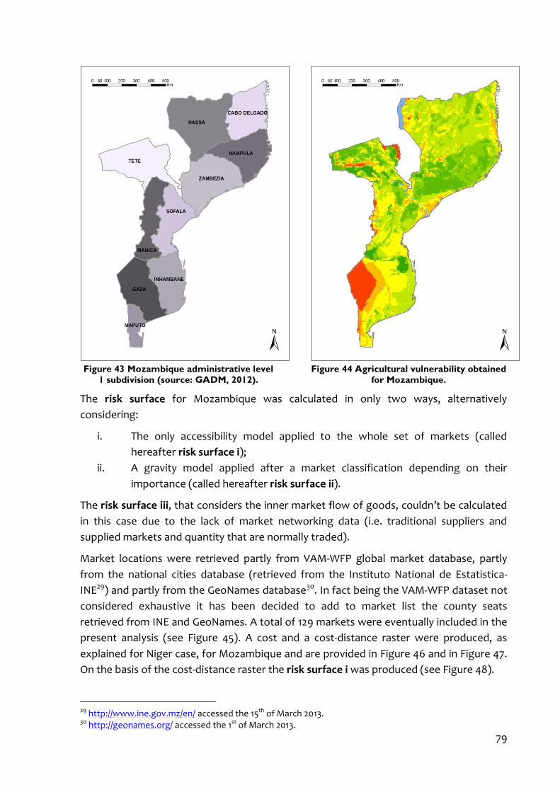
79
Figure 43 Mozambique administrative level
1 subdivision (source: GADM, 2012).
Figure 44 Agricultural vulnerability obtained
for Mozambique.
The risk surface for Mozambique was calculated in only two ways, alternatively
considering:
i. The only accessibility model applied to the whole set of markets (called
hereafter risk surface i);
ii. A gravity model applied after a market classification depending on their
importance (called hereafter risk surface ii).
The risk surface iii, that considers the inner market flow of goods, couldn’t be calculated
in this case due to the lack of market networking data (i.e. traditional suppliers and
supplied markets and quantity that are normally traded).
Market locations were retrieved partly from VAM-WFP global market database, partly
from the national cities database (retrieved from the Instituto National de Estatistica-
INE29) and partly from the GeoNames database30. In fact being the VAM-WFP dataset not
considered exhaustive it has been decided to add to market list the county seats
retrieved from INE and GeoNames. A total of 129 markets were eventually included in the
present analysis (see Figure 45). A cost and a cost-distance raster were produced, as
explained for Niger case, for Mozambique and are provided in Figure 46 and in Figure 47.
On the basis of the cost-distance raster the risk surface i was produced (see Figure 48).
29 http://www.ine.gov.mz/en/ accessed the 15th of March 2013. 30 http://geonames.org/ accessed the 1st of March 2013.
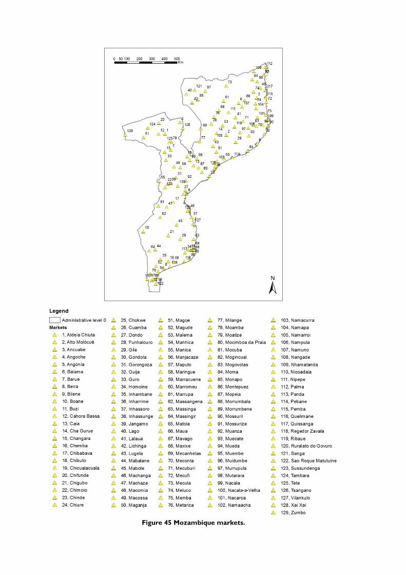
Figure 45 Mozambique markets.

81
Figure 46 Mozambique cost raster.
Figure 47 Cost distance calculated for 129
Mozambique markets.
Figure 48 Risk surface calculated on the
basis of the accessibility to Mozambique
main markets (i.e. risk surface i).
Figure 49 Risk surface calculated with the
Huff gravity model for Mozambique main
markets (i.e. risk surface ii).
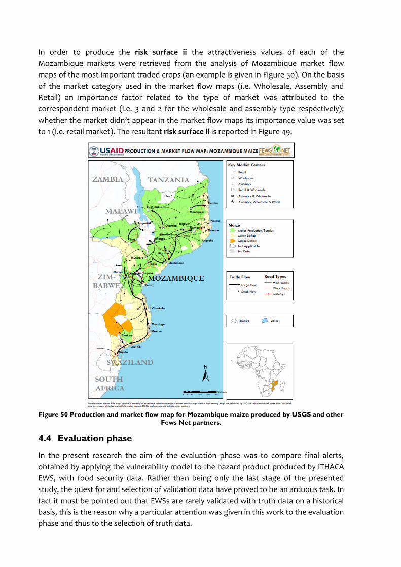
In order to produce the risk surface ii the attractiveness values of each of the
Mozambique markets were retrieved from the analysis of Mozambique market flow
maps of the most important traded crops (an example is given in Figure 50). On the basis
of the market category used in the market flow maps (i.e. Wholesale, Assembly and
Retail) an importance factor related to the type of market was attributed to the
correspondent market (i.e. 3 and 2 for the wholesale and assembly type respectively);
whether the market didn’t appear in the market flow maps its importance value was set
to 1 (i.e. retail market). The resultant risk surface ii is reported in Figure 49.
Figure 50 Production and market flow map for Mozambique maize produced by USGS and other
Fews Net partners.
4.4 Evaluation phase
In the present research the aim of the evaluation phase was to compare final alerts,
obtained by applying the vulnerability model to the hazard product produced by ITHACA
EWS, with food security data. Rather than being only the last stage of the presented
study, the quest for and selection of validation data have proved to be an arduous task. In
fact it must be pointed out that EWSs are rarely validated with truth data on a historical
basis, this is the reason why a particular attention was given in this work to the evaluation
phase and thus to the selection of truth data.

83
In particular if one aims at validating a drought EWS, he will encounter the following
issues: firstly, drought impacts are various thus not univocally recognized and measured;
secondly historical impact data, aggregated on the basis of a more detailed level than the
country one, are rarely available; thirdly, when data at sub-country level exist, they are
rarely organized in geospatial well-structured databases and are frequently produced by
different sources.
The first mentioned issue was addressed by deciding to use food security data as impact
data, targeting one of the main indirect shocks caused by drought. Second and third
issues were solved by using regional food security outlooks produced as maps with a
common interpreting scale since 2008, thus usable for qualitative evaluation purposes for
different countries, and locally retrieved food security data aggregated at second
administrative subdivision, usable only in particular cases.
Eventually for the purpose of validating the Final Alerts two types of data were used:
Food Security Outlook and Assessments produced by Fews Net, that have been
used for a qualitative evaluation (see 4.4.1);
Food Security Assessments (FSA) produced by WFP Niger offices, which have
been used for a quantitative evaluation in the Niger case (see 4.4.2).
4.4.1 Qualitative evaluation
In order to perform a qualitative evaluation of produced final alerts, Fews Net Food
Security Assessments and Outlooks were used. The aim of the qualitative evaluation is to
compare the two products (i.e. Fews Net Outlooks and Final Alerts of the presented
model combined with ITHACA EWS hazard). The comparison is performed year per year
for the available time series (further details are found in section 5.1).
The Fews Net project has the primary mandate to produce famine early warning outputs.
Fews Net is the only global provider of famine assessments and outlooks. On the project
website18F
31 these outlooks are made available on quarterly basis, providing food security
conditions for the coming three to six months (an example is provided in Figure 12). These
data are available as text bulletin and as shapefiles with regional and, less frequently,
country extent. Fews Net classification is here considered useful because: (i) areas
classified do not normally follow any administrative boundary; (ii) food security projected
severity is classified according to the Integrated Food Security Phase Classification (IPC
2.0)19F
32 scale; (iii) it is the only global monitoring system that provides maps outlining the
degree of food security and its extent; (iv) the same methodology is used for producing
famine alerts for different countries, thus allowing comparing the food security situation
of those different countries and regions. Moreover, the IPC scale is widely accepted by
the humanitarian community and offers classification standards that permit users
worldwide to understand and use a common reference language. The reference table for
31 http://www.fews.net/ 32 http://www.fews.net/our-work/our-work/integrated-phase-classification
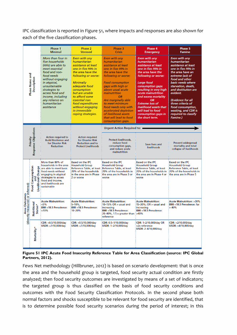
IPC classification is reported in Figure 51, where impacts and responses are also shown for
each of the five classification phases.
Figure 51 IPC Acute Food Insecurity Reference Table for Area Classification (source: IPC Global
Partners, 2012).
Fews Net methodology (Hillbruner, 2012) is based on scenario development: that is once
the area and the household group is targeted, food security actual condition are firstly
analyzed; then food security outcomes are investigated by means of a set of indicators;
the targeted group is thus classified on the basis of food security conditions and
outcomes with the Food Security Classification Protocols. In the second phase both
normal factors and shocks susceptible to be relevant for food security are identified, that
is to determine possible food security scenarios during the period of interest; in this

85
phase various assumptions about timing, duration and severity of likely shocks have to be
made. At this point expected impacts on income and food sources of the targeted group
should be identified. The next stage implies the identification of group responses to the
identified shocks impacting food access and earnings. Eventually, projected food security
conditions and areas are classified and described through the Food Security Classification
Protocols.
4.4.2 Quantitative evaluation
One of the most challenging issues of the presented work is the validation of the
produced outputs. As a matter of fact a verified accordance with truth data should be
considered essential in the developing of monitoring and early warning systems.
Unfortunately, due to objective difficulty of the drought impact definition and
consequently lack of truth data, existing EWS are seldom if ever validated. In the present
case it turned out to be very difficult to find quantitative data related to measured food
security at global extent, which is the indirect drought impact targeted by the present
study. In addition, even when country-specific datasets are to be considered, they happen
to be rarely accessible remotely. Eventually, a field mission was deemed necessary to
retrieve historical food security data at sub-country level. WFP Niger bureau hosted the
author for a month permitting data collection and furnishing unavoidable interpretation
support provided by the local staff.
Therefore the quantitative evaluation was conducted with data resuming food insecurity
conditions for Niger administrative level 2 subdivisions (Food Security Assessments, FSA)
retrieved locally. These data are produced yearly, when field security conditions are met,
by the WFP country office on the basis of field surveys. A set of target households is
constantly monitored in order to measure 5 indicators (i.e. called “active indicators”):
Food consumption score;
Coping strategy index ;
Share of expenditure devoted to food;
Tropical Livestock Units (TLUs) owned;
Duration of food stock.
Following the data collection, a Principal Component Analysis (PCA) is performed in order
to identify indicator values that describe analogous food security conditions. The PCA
allows to: determine households groups characterized by the same food security status,
and to classify these groups on the basis of their level of food security. As a result the
population of each department (departments of Niger are reported in Figure 52), after
extrapolation, is categorized in classes of food insecurity, i.e. (i) percentage of food
secure; (ii) percentage of moderate food insecure; (iii) percentage of severe food
insecure.
FSA data are used by the local WFP staff to target the beneficiaries and the extent of WFP
interventions. The assessments are conducted monthly but evaluated and used or at the
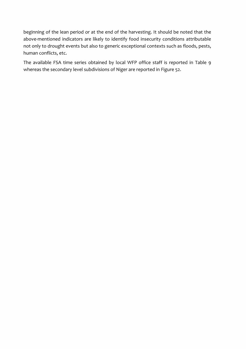
beginning of the lean period or at the end of the harvesting. It should be noted that the
above-mentioned indicators are likely to identify food insecurity conditions attributable
not only to drought events but also to generic exceptional contexts such as floods, pests,
human conflicts, etc.
The available FSA time series obtained by local WFP office staff is reported in Table 9
whereas the secondary level subdivisions of Niger are reported in Figure 52.

87
Table 9 Food Security Assessment data for Niger departments. Values are expressed in affected population percentage. 2013 values are estimation as of
October 2013 and are not retrieved from field surveys.
2006 2007 2008 2009 2011 2013
Department Moderate Severe Total Moderate Severe Total Moderate Severe Total Moderate Severe Total Moderate Severe Total Total
Aguie 21,8 1 22,8 5,5 8,9 14,4 18,8 4,1 22,9 28,3 34,1 62,4 19,1 6,6 25,7 44,0
Arlit 32,1 9,7 41,8 N.A. N.A. N.A. 20,9 5 25,9 N.A. N.A. N.A. N.A. N.A. N.A. 13,4
Bilma 17,2 0,5 17,7 N.A. N.A. N.A. N.A. N.A. N.A. N.A. N.A. N.A. N.A. N.A. N.A. N.A.
Birni N'gaoure 22,5 13,8 36,3 24,1 14,3 38,4 14,4 6,4 20,8 39,9 5,8 45,7 16,2 4,4 20,6 26,7
Birni N'konni 14,7 2,1 16,8 25 3,1 28,1 15,9 7,3 23,2 21,5 8,4 29,9 12,5 5,6 18,1 30,4
Bouza 34,9 7,1 42 48,1 6,6 54,7 31,9 10,7 42,6 15,5 37,6 53,1 33,7 13,6 47,3 46
Dakoro 15,9 10,2 26,1 5,3 18,7 24 3,6 2,6 6,2 27,5 12 39,5 12,9 4,2 17,1 15,6
Diffa 5,3 0,6 5,9 41,4 7,3 48,7 18,4 17,3 35,7 22,4 10,3 32,7 29,6 5 34,6 8,8
Dogondoutchi 19,4 1,4 20,8 17 13,1 30,1 8,6 1,7 10,3 25,8 14,9 40,7 21 4,2 25,2 54,4
Dosso 26,9 3,7 30,6 24,1 14,3 38,4 22,7 7,2 29,9 32,9 18,6 51,5 31,2 1,4 32,6 30,9
Filingue 23,1 5,1 28,2 37,2 15,5 52,7 14,2 4,9 19,1 27,2 17,8 45 31,2 9,6 40,8 20
Gaya 6,4 2,6 9 24,1 14,3 38,4 19,5 5,5 25 20,7 8,6 29,3 17,4 1 18,4 49,4
Goure 14,7 16 30,7 33,2 11,8 45 13,3 13 26,3 17,9 6,1 24 23,6 7,2 30,8 25,5
Guidan Roumji 22,4 10,9 33,3 20,4 16 36,4 21,2 8,4 29,6 29,7 26 55,7 23,2 3,5 26,7 26,1
Illela 24,5 14,8 39,3 14 9 23 22,2 21,1 43,3 27 19,3 46,3 23,4 15,5 38,9 62,2
Keita 18,7 33,2 51,9 42,7 15,2 57,9 28,9 17,2 46,1 19,6 37,1 56,7 30 10,6 40,6 54,5
Kollo 19,5 1,5 21 21,6 24,7 46,3 17,8 7,2 25 36,1 17,3 53,4 32,2 8,3 40,5 17,8
Loga 31,2 16,9 48,1 24,1 14,3 38,4 10,5 2,6 13,1 30,4 14,1 44,5 34,4 9,5 43,9 44,2
Madaoua 18,9 6 24,9 9,2 8,8 18 15,6 10,6 26,2 27 28,7 55,7 30,7 1,1 31,8 35,2
Madarounfa 15,4 8,7 24,1 8 8,4 16,4 9,8 3,3 13,1 31 25,9 56,9 15,4 5,2 20,6 31,9
Magaria 15,1 6,4 21,5 33,8 13 46,8 12,8 5,9 18,7 34,3 9,9 44,2 40,4 2,3 42,7 7,9
Maine-soroa 20,2 1,6 21,8 N.A. N.A. N.A. 16,8 11,5 28,3 21,8 23,3 45,1 29,3 8,8 38,1 12
Matamey 11,8 3 14,8 20,1 8,9 29 21,8 8,5 30,3 20,8 13,5 34,3 25,2 2,2 27,4 9,4
Mayahi 25,6 0 25,6 11,3 9,6 20,9 10,1 2,8 12,9 23,3 26,6 49,9 28,4 11,5 39,9 27,0

Miria 20,4 12,8 33,2 16,3 9,5 25,8 19,2 7,8 27 27,1 14,9 42 18,6 4,2 22,8 26,6
N'guigmi 20,4 1,1 21,5 N.A. N.A. N.A. 10 13 23 10,8 6,7 17,5 25,2 1,7 26,9 1,9
Niamey 24,3 1,5 25,8 17,5 18,4 35,9 12,8 14,9 27,7 36,4 6,5 42,9 22 7,3 29,3 N.A.
Ouallam 17 40,8 57,8 14,5 33 47,5 18,2 13,7 31,9 20,5 64,1 84,6 27,5 13,1 40,6 33,8
Say 20 1,5 21,5 8,5 15,1 23,6 2,3 2,6 4,9 25,2 1,6 26,8 9,5 7 16,5 36,9
Tahoua 19,5 31,9 51,4 32,2 5,5 37,7 5,3 7,8 13,1 31,4 28,9 60,3 26,9 9,9 36,8 30,1
Tanout 46,7 4,7 51,4 13 4,9 17,9 4,8 8,1 12,9 31,4 29,3 60,7 53,5 3,5 57 23,6
Tchighozerine 15,6 5,2 20,8 9,1 13,9 23 24,8 35,3 60,1 N.A. N.A. N.A. N.A. N.A. N.A. 18,9
Tchin Tabaradene 29 12,1 41,1 34 9,3 43,3 21,7 51,9 73,6 12,8 12,2 25 14,5 4,9 19,4 39,7
Tera 19,8 2 21,8 32,2 9,2 41,4 16,3 25,4 41,7 27,2 17,2 44,4 32,4 8,7 41,1 54,1
Tessaoua 10,5 5,5 16 15,7 7 22,7 18,5 22,8 41,3 20,6 56,9 77,5 27,6 9 36,6 19,5
Tillaberi 26 33,9 59,9 14 5,1 19,1 15 33,1 48,1 31,2 32,4 63,6 14,6 8,3 22,9 31,6

89
FSA data of 2010 are lacking due to the military coup occurred the same year in January,
that most probably made impossible to conduct field surveys for the whole year. Data
from Arlit and Bilma departments are also lacking for almost the whole time series due to
the security issues persistent in the desert region in the Northern part of the country.
Figure 52 Niger administrative level 2 subdivision (i.e. departments).

5 RESULTS
In this chapter the results of the evaluation process of the final alerts (hereafter called
“model alerts” as well) are presented. In the first section the results of the qualitative
evaluation are presented while in the second section the quantitative one is presented. A
third section is devoted to the discussion of both types of evaluation assessments.
5.1 Qualitative evaluation
The qualitative evaluation was performed by means of Fews Net products (refer to
paragraph 4.4.1 for more details). The final alerts, produced by applying the vulnerability
model to the hazard produced by ITHACA, were compared with Fews Net maps produced
from 2008 to 2013. Both case studies were considered in the qualitative evaluation
process and the three risk surfaces were evaluated as well (i.e. risk surface i calculated on
the basis of the easiness to reach marketplaces; risk surface ii which exploits a spatial
gravity model; risk surface iii that integrates the gravity model with market trade
information).
Three types of outputs are produced periodically by Fews Net: food security current
conditions, food security outlook and food security updates. The first states the actual
food security conditions, the second provides projections of food security conditions on
the three to six next months on the basis of both most likely and worst future scenarios;
while the third type provides updates of an already disseminated outlook on the basis of
occurred changes in food security conditions. Considering that the final alerts, produced
with the application of the presented vulnerability model to the case studies, are
calculated taking into account the whole vegetation growing season, i.e. at the end of it,
it has been decided to use the three types of Fews Net products according to the period
in which they were produced and made public. When available, the priority of use was
given to food security current conditions or updates that, instead of being based on
projected assumptions, are the outcomes of field indicator analysis.
A selection of model alert maps and of food security outlook is provided in the following
paragraphs, grouped per country and per year. The alert values obtained with the model
are expressed in the same unit in which the NDVI anomalies are expressed (percentage of
anomaly with respect to the average of the time series) while Fews Net map values are
expressed through the IPC scale (for more details see Figure 51).
Fews Net maps have been downloaded as bulletin in pdf formats from ReliefWeb
website20F
33; the available bulletin time series starts from 2008, so does the qualitative
evaluation.
33 http://reliefweb.int/

91
Niger food security 2008
Figure 53 Food security assessment as of July 2008 (FEWS NET).
Figure 54 Model alert for 2008 harvest season for risk surface i.
Figure 55 Model alert for 2008 harvest season for risk surface ii.
Figure 56 Model alert for 2008 harvest season for risk surface iii.

Niger food security 2009
Figure 57 Food security assessment as of January 2010 (FEWS NET).
Figure 58 Model alert for 2009 harvest season for risk surface i.
Figure 59 Model alert for 2009 harvest season for risk surface ii.
Figure 60 Model alert for 2009 harvest season for risk surface iii.
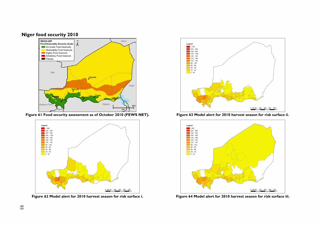
93
Niger food security 2010
Figure 61 Food security assessment as of October 2010 (FEWS NET).
Figure 62 Model alert for 2010 harvest season for risk surface i.
Figure 63 Model alert for 2010 harvest season for risk surface ii.
Figure 64 Model alert for 2010 harvest season for risk surface iii.

Niger food security 2011
Figure 65 Food security assessment as of Sept. 2011 (FEWS NET).
Figure 66 Model alert for 2011 harvest season for risk surface i.
Figure 67 Model alert for 2011 harvest season for risk surface ii.
Figure 68 Model alert for 2011 harvest season for risk surface iii.

95
Niger food security 2012
Figure 69 Food security assessment as of October 2012 (FEWS NET).
Figure 70 Model alert for 2012 harvest season for risk surface i.
Figure 71 Model alert for 2012 harvest season for risk surface ii.
Figure 72 Model alert for 2012 harvest season for risk surface iii.

Niger food security 2013
Figure 73 Food security assessment as of January 2014 (FEWS NET).
Figure 74 Model alert for 2013 harvest season for risk surface i.
Figure 75 Model alert for 2013 harvest season for risk surface ii.
Figure 76 Model alert for 2013 harvest season for risk surface iii.

97
Mozambique food security 2008
Figure 77 Food security assessment as of
August 2008 (FEWS NET).
Figure 78 Model alert for 2008 harvest
season for risk surface i.
Figure 79 Model alert for 2008 harvest
season for risk surface ii.

Mozambique food security 2009
Figure 80 Food security assessment as of
March 2009 (FEWS NET).
Figure 81 Model alert for 2009 harvest
season for risk surface i.
Figure 82 Model alert for 2009 harvest
season for risk surface ii.
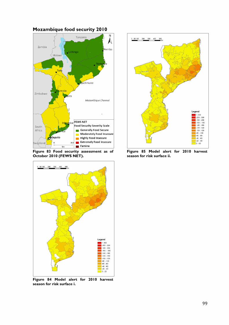
99
Mozambique food security 2010
Figure 83 Food security assessment as of
October 2010 (FEWS NET).
Figure 84 Model alert for 2010 harvest
season for risk surface i.
Figure 85 Model alert for 2010 harvest
season for risk surface ii.

Mozambique food security 2011
Figure 86 Food security assessment as of
March 2011 (FEWS NET).
Figure 87 Model alert for 2011 harvest
season for risk surface i.
Figure 88 Model alert for 2011 harvest
season for risk surface ii.
101
Mozambique food security 2012
Figure 89 Food security assessment as of
June 2012 (FEWS NET).
Figure 90 Model alert for 2012 harvest
season for risk surface i.
Figure 91 Model alert for 2012 harvest
season for risk surface ii.

Mozambique food security 2013
Figure 92 Food security assessment as of
March 2013 (FEWS NET).
Figure 93 Model alert for 2013 harvest
season for risk surface i.
Figure 94 Model alert for 2013 harvest
season for risk surface ii.

103
5.2 Quantitative evaluation
In order to perform a quantitative evaluation, by means of the use of FSA data (refer to
paragraph 4.4.2 for more details about these data), it has been necessary to recalculate
the average model alert values per administrative level 2. In fact the alert values
produced by the model are given per risk surface units which don’t correspond with the
administrative boundaries (Figure 95). This operation was performed mainly with the
Tabulate Intersection tool, which is available in the Geoprocessing toolbox of ArcGis (i.e.
the tool computes the intersection between two feature classes and cross-tabulates the
area of, length of, or count the intersecting features).
Figure 95 On the left the administrative level 2 of Niger, on the right the risk surface i calculated
for Niger.
After the recalculation of the model alerts according to the administrative level 2
subdivisions, both FSA and final alert time series were then standardized over the
available time series in order to make them comparable. What have been analyzed, and
discussed in the following paragraphs, are not the single yearly values of the two datasets
compared but their variations from one year to the next. As a matter of fact the absolute
values of the final alert produced are considered so far less important than the correct
interpretation of crisis within the proposed model.
A selection of the evaluation results of the model applied to the three type of risk
surfaces is presented in the following, aggregated per department and per year, in order
to provide an overview of cases in which the model worked properly and less well.
For the three risk surfaces the departments showing the best and worst results are
presented, the graphs representing the comparison between FSA and model alert
standardized values are reported from Figure 96 to Figure 103.
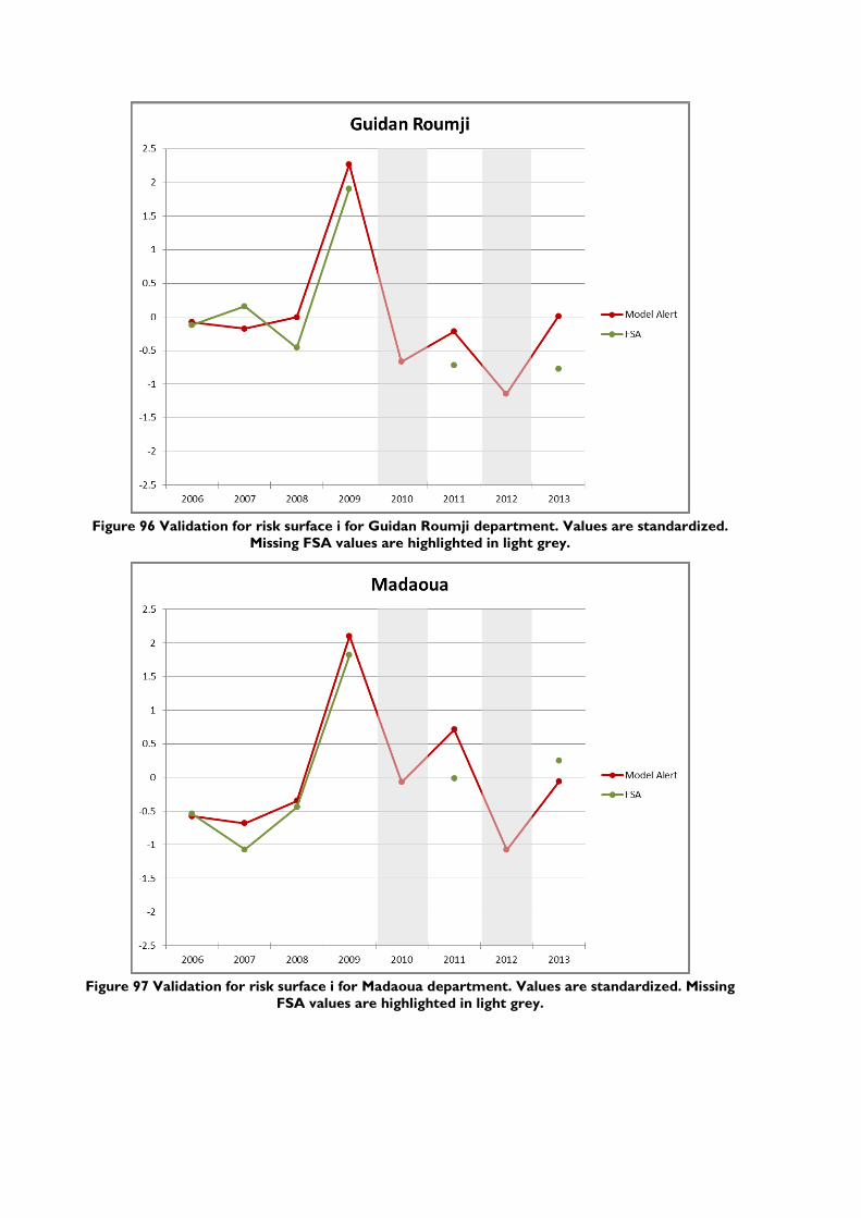
Figure 96 Validation for risk surface i for Guidan Roumji department. Values are standardized.
Missing FSA values are highlighted in light grey.
Figure 97 Validation for risk surface i for Madaoua department. Values are standardized. Missing
FSA values are highlighted in light grey.

105
Figure 98 Validation for risk surface ii for Miria department. Values are standardized. Missing
FSA values are highlighted in light grey.
Figure 99 Validation for risk surface ii for Madaoua department. Values are standardized. Missing
FSA values are highlighted in light grey.

Figure 100 Validation for risk surface i for Tchin Tabaradene department. Values are
standardized. Missing FSA values are highlighted in light grey.
Figure 101 Validation for risk surface i for Birni N’konni department. Values are standardized.
Missing FSA values are highlighted in light grey.
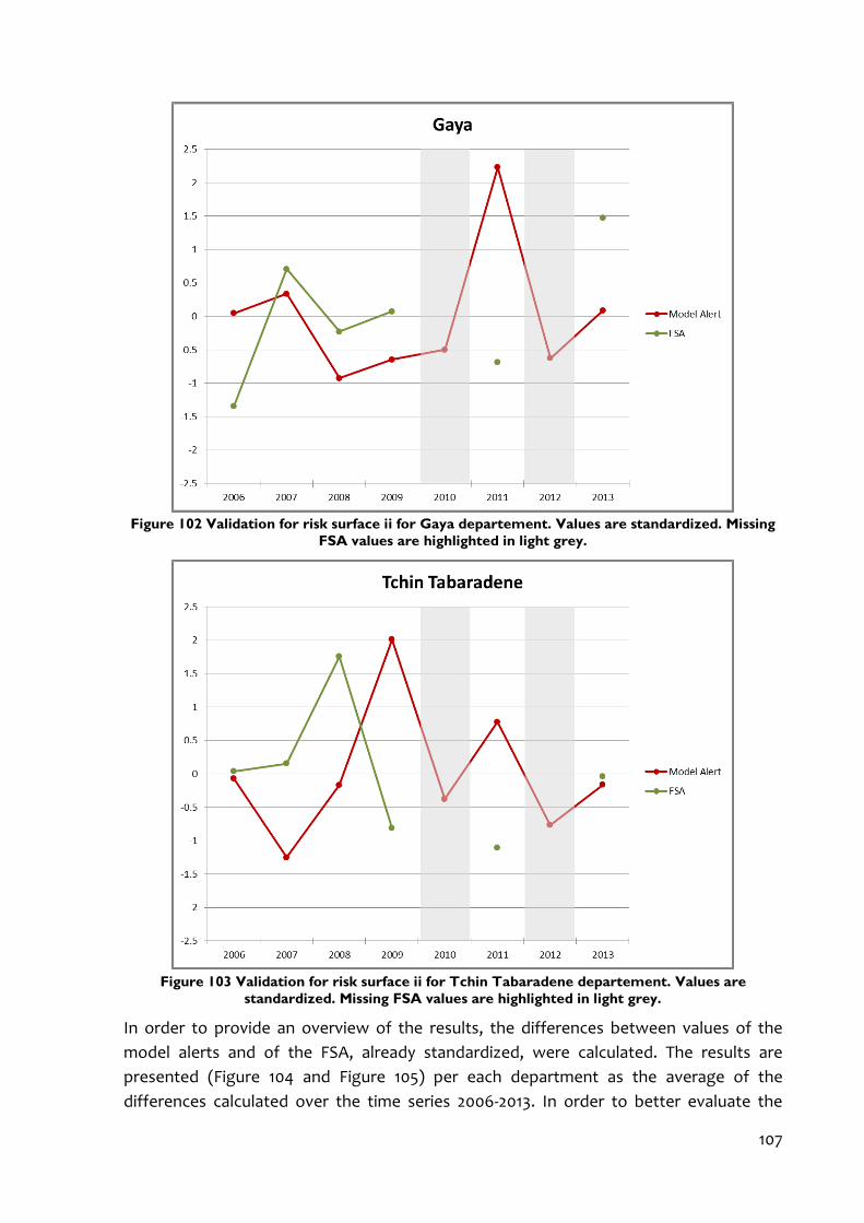
107
Figure 102 Validation for risk surface ii for Gaya departement. Values are standardized. Missing
FSA values are highlighted in light grey.
Figure 103 Validation for risk surface ii for Tchin Tabaradene departement. Values are
standardized. Missing FSA values are highlighted in light grey.
In order to provide an overview of the results, the differences between values of the
model alerts and of the FSA, already standardized, were calculated. The results are
presented (Figure 104 and Figure 105) per each department as the average of the
differences calculated over the time series 2006-2013. In order to better evaluate the

model alerts it has been decided to recalculate those alerts by applying the agricultural
vulnerability to the considered hazard and aggregating the results per administrative
level 2 (departments). This was done in order to evaluate the significance of the three
proposed risk surfaces through the comparison of original final alerts with those obtained
by using the model without any of the risk surfaces; results are shown in Figure 106.
Figure 104 The graph presents the mean of the differences between the Model Alerts (Risk
surface i) and the FSA calculated over the period 2006-2013 per department.
Figure 105 The graph presents the mean of the differences between the Model Alerts (Risk
surface ii) and the FSA calculated over the period 2006-2013 per department.
Figure 106 The graph presents the mean of the differences between the Model Alerts
(Administrative level 2) and the FSA calculated over the period 2006-2013 per department.
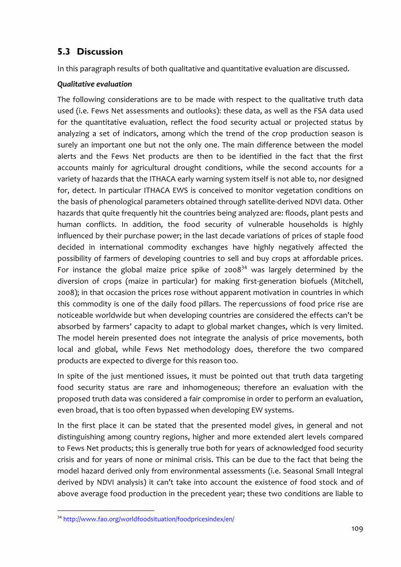
109
5.3 Discussion
In this paragraph results of both qualitative and quantitative evaluation are discussed.
Qualitative evaluation
The following considerations are to be made with respect to the qualitative truth data
used (i.e. Fews Net assessments and outlooks): these data, as well as the FSA data used
for the quantitative evaluation, reflect the food security actual or projected status by
analyzing a set of indicators, among which the trend of the crop production season is
surely an important one but not the only one. The main difference between the model
alerts and the Fews Net products are then to be identified in the fact that the first
accounts mainly for agricultural drought conditions, while the second accounts for a
variety of hazards that the ITHACA early warning system itself is not able to, nor designed
for, detect. In particular ITHACA EWS is conceived to monitor vegetation conditions on
the basis of phenological parameters obtained through satellite-derived NDVI data. Other
hazards that quite frequently hit the countries being analyzed are: floods, plant pests and
human conflicts. In addition, the food security of vulnerable households is highly
influenced by their purchase power; in the last decade variations of prices of staple food
decided in international commodity exchanges have highly negatively affected the
possibility of farmers of developing countries to sell and buy crops at affordable prices.
For instance the global maize price spike of 200834 was largely determined by the
diversion of crops (maize in particular) for making first-generation biofuels (Mitchell,
2008); in that occasion the prices rose without apparent motivation in countries in which
this commodity is one of the daily food pillars. The repercussions of food price rise are
noticeable worldwide but when developing countries are considered the effects can’t be
absorbed by farmers’ capacity to adapt to global market changes, which is very limited.
The model herein presented does not integrate the analysis of price movements, both
local and global, while Fews Net methodology does, therefore the two compared
products are expected to diverge for this reason too.
In spite of the just mentioned issues, it must be pointed out that truth data targeting
food security status are rare and inhomogeneous; therefore an evaluation with the
proposed truth data was considered a fair compromise in order to perform an evaluation,
even broad, that is too often bypassed when developing EW systems.
In the first place it can be stated that the presented model gives, in general and not
distinguishing among country regions, higher and more extended alert levels compared
to Fews Net products; this is generally true both for years of acknowledged food security
crisis and for years of none or minimal crisis. This can be due to the fact that being the
model hazard derived only from environmental assessments (i.e. Seasonal Small Integral
derived by NDVI analysis) it can’t take into account the existence of food stock and of
above average food production in the precedent year; these two conditions are liable to
34 http://www.fao.org/worldfoodsituation/foodpricesindex/en/
increase the food security level of households. Another possible explanation, valid in
particular for the case of Mozambique, is that very short growing seasons (e.g. lasting
one or two months) are not detected by ITHACA vegetation anomaly monitoring system.
It happens that the seasonal crop calendar for Mozambique (see Figure 42) is
characterized by two planting and harvesting seasons in the southern regions of the
country. This could cause the inconsistency of the model alerts with respect to the Fews
Net assessment, as the latter takes into account the whole yearly production and not the
one produced during the only main crop season. It should also be pointed out that no
threshold value is fixed on the alerts retrieved by ITHACA vegetation anomaly monitoring
system, thus all the anomalies detected are categorized and reported in the output
products. An analysis of further case studies would permit to identify a threshold value in
order to distinguish between false alerts (i.e. small values to be considered negligible)
and true ones.
Secondarily if one considers years 2008, 2009 and 2010 (from Figure 53 to Figure 64)
some considerations can be made about the differences in the functioning of the model
with respect to the three type of risk surfaces tested on the Niger case study: the model
using risk surface i provides good outputs for the southern regions of the country, so it
does the model using risk surface ii, whilst both the models fail to provide alerts over the
northern regions. Southern regions (in particular the south-eastern ones) are those
characterized by the major presence of cultivated land so as to be called the wheat belt
(le grenier du Pays, in french), while northern regions are characterized by the presence of
the desert and thus of an environment unfitting to cultivations. Given the fact that the
agricultural vulnerability surface is calculated only for those pixels identified as
agricultural land and that all the further calculations are based on this primary distinction
between cultivated and non-cultivated land, it is clear that the northern desert areas are
almost never screened for food security alerts. However, in the case of the model using
risk surface iii, the risk units of northern Niger are provided with an alert for each of the
years that were considered in the analysis. In fact markets of the northern regions, such
as Agadez, Arlit or Bilma (refer to Figure 38 for market location and to Figure 52 for
administrative level 2 subdivisions), are evidently supplied by the southern markets
located in food production surplus areas. The latter is confirmed by the analysis of the
local market database in which the food trades data are stored and described (see Table
7). When building risk surface iii the interrelations among markets were considered,
therefore part of the staple production drop that occurs in the wheat belt is reflected in
the northern regions, which are not autonomous with respect to food production.
The latter consideration proves the model to be useful when a specific country is
analyzed. However the application of a country-tailored vulnerability model based on
local market network information would be difficult to be implemented at global extent,
which is the target extent of the ITHACA EWS for drought.

111
Quantitative evaluation
The results of the quantitative evaluation are highly variable from one department to
another and from one year to another as well. The generic considerations (i.e. short
available time-series, evaluation data not drought specific) made for the data used for the
qualitative evaluation are valid for the FSA evaluation data as well; they could be the main
factors leading the differences revealed by the comparison. However it must be
remembered that quantitative data regarding food security conditions are rarely
produced and made available; this is the reason why FSA data were nevertheless used for
evaluative purposes.
Firstly it must be pointed out that the performances of the model which uses the risk
surface i and those of the model using the risk surface ii don’t differ significantly. One of
the reason can be found in the fact that the two risk surfaces are geographically similar
because the basic choice of importance factors inserted in the gravity spatial model (i.e.
3, 2, 1 values assigned to wholesale, assembly and retail markets respectively), used to
build the risk surface ii, was the only tested option. The case of the model which uses the
risk surface iii would reasonably give rather different results, however it was decided not
to evaluate them considering that the assumptions made to build this risk surface iii were
quite arbitrary and primarily needed in order to test the option but are not considered
valuable from the quantitative point of view.
The results of the evaluation process for the departments of Madaoua and Guidan
Roumji, obtained with the risk surface i, show good correspondences between the two
data series (see Figure 96 and Figure 106). However it appears that 2007, 2011 and 2013
are the years for which the model alerts differ more from the FSA data. Madaoua
department shows the best results among the others also when the model using the risk
surface ii is considered (see Figure 99). A good performance was proven also for the
Miria department in this second case (see Figure 98). The same three years affect
negatively the overall results of the model that uses the risk surface ii as well. If one
analyses the hazard occurrences for those years, it finds no particular causes that could
have affected the food security in the country. It can be eventually said that these three
departments (i.e. Miria, Guidan Roumji, Madaoua) are located in the southern part of the
country where most of the croplands is, this fact could explain the overall good
performance of the model in the area.
The model, both when using risk surface i and risk surface ii, provides controversial
results for the following departments: Tchin Tabaradene, Birni N’konni and Gaya (see
from Figure 100 to Figure 103). The model alerts differ considerably from the FSA data
and in a comparable way for all years of the time series. As long as Tchin Tabaradene is
concerned a possible explanation of the wrong alerts associated with this department is
the fact that it is situated nearby the desert and thus the alerts provided by the model
don’t represent properly a land with none or minimal cropland (see Figure 107). For what
concerns the departments of Birni N’konni and Gaya it is likely that, as they rely on
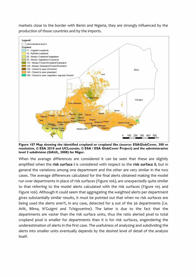
markets close to the border with Benin and Nigeria, they are strongly influenced by the
production of those countries and by the imports.
Figure 107 Map showing the identified cropland or cropland like (source: ESAGlobCover, 300 m
resolution, © ESA 2010 and UCLouvain, © ESA / ESA GlobCover Project) and the administrative
level 2 subdivision (GAUL, 2008) for Niger.
When the average differences are considered it can be seen that these are slightly
amplified when the risk surface i is considered with respect to the risk surface ii, but in
general the variations among one department and the other are very similar in the two
cases. The average differences calculated for the final alerts obtained making the model
run over departments in place of risk surfaces (Figure 106), are unexpectedly quite similar
to that referring to the model alerts calculated with the risk surfaces (Figure 105 and
Figure 106). Although it could seem that aggregating the weighted alerts per department
gives substantially similar results, it must be pointed out that when no risk surfaces are
being used the alerts aren’t, in any case, detected for 4 out of the 36 departments (i.e.
Arlit, Bilma, N’Guigmi and Tchigozerine). The latter is due to the fact that the
departments are vaster than the risk surface units, thus the ratio alerted pixel to total
cropland pixel is smaller for departments than it is for risk surfaces, engendering the
underestimation of alerts in the first case. The usefulness of analyzing and subdividing the
alerts into smaller units eventually depends by the desired level of detail of the analysis
itself.
113
CONCLUSIONS AND FURTHER DEVELOPMENTS
The research targeted the complex aim of defining a vulnerability model to be integrated
into an existing early warning system for drought. The need of integrating vulnerability
for measuring risk towards natural hazards, especially in the case of drought, was stated
both by international agencies dealing with disaster reduction (UN/ISDR, 2004a; UNDP,
2004) and by the scientific community (W. Neil Adger, 2006; S. L. Cutter, Boruff, & Shirley,
2003; Susan L. Cutter, 1996). It has also been authoritatively declared that the process for
make the vulnerability information available and accessible to the profit of engineers,
planners and policy-makers is in the current agenda of the international community
working for the creation of disaster resilient societies (UN, 2006).
In order to build the model, existing system for drought risk assessment were
investigated (Birkmann & Mucke, 2011; Peduzzi et al., 2009; Wilcox et al., n.d.), as well as
recommendations for building indicators to assess people’s vulnerability to droughts
(Eriygama et al., 2009; Julich, 2006; Miller et al., 2002) were considered.
Starting from the hazard data provided by a specific drought monitoring system (i.e.
NDVI-based seasonal vegetation anomalies calculated on a 5km grid) it has been decided
to add to the system both agricultural specific and socio-economic vulnerability factors.
The introduction of vulnerability factors has the objective of translating the
environmental hazard into impacts on population. The change in food security conditions
was targeted as the main indirect impact produced by drought conditions detected by
the vegetation anomaly monitoring system.
The proposed vulnerability model is conceived as relying on two surfaces, i.e. the
agricultural vulnerability surface and the risk surface; the first one accounts for the
peculiar vulnerability of a cropland to drought conditions and is constituted of three
indicators (i.e. the soil suitability for crop production, the percentage of irrigation areas
and the crop diversity index); the second surface tries to depict the linkage between
areas hit by vegetation stress and areas where the impacts on the population may occur.
The concept of risk surface is considered promising for it aims at translating the proved
territorial relations between hazard and impacts into a spatial connection. It happens that
these connections are renowned though not systematically analyzed in a GIS framework
that set them for their transparent and objective use (Hillbruner, 2012). Three types of risk
surfaces were tested and evaluated: (i) one obtained by implementing an accessibility
model that takes into account the easiness to reach marketplaces; (ii) a second one
obtained by applying a gravity model for user spatial choice among markets on the basis
of each market influence; (iii) a third one in which the gravity model is combined with
national market flow of goods.
A preliminary consideration regarding the three tested risk surfaces is the following: it
can be inferred by examining the risk surface of first and second type that the differences

between them are, sometimes, slight. This can be due to the author’s choice in attributing
the attractiveness factors of the implemented gravity model. As stated in previous study
more attention should be devoted to the attribution of the attractiveness factors that, in
the original Huff’s probability function (see eq. [5]) were the size of the stores, and in the
proposed model were replaced with the market importance factors. It must be said that
the application attempts of consumers’ choice models at the country level and in the
context of developing countries are almost null; therefore necessary adaptations of these
spatial models have still to be studied and verified.
The three resulting versions of the model, each obtained by using one of the three risk
surfaces at a time, were applied to the hazard detected for two national case studies in
the time frame 2006-2013: Niger and Mozambique. The final outputs, i.e. hazard values
weighted with agricultural vulnerability and distributed over the risk surfaces, were
evaluated qualitatively and quantitatively. The qualitative evaluation, performed in both
cases, was made through the yearly comparison of the Final Alerts with the Fews Net
products (food security assessment and outlooks maps) over the period 2008-2013. The
quantitative evaluation was performed only in the case of Niger, by means of food
security field survey data (i.e. WFP Food Security Assessment, FSA) of 2006-2013 that
were retrieved by the author from WFP Niger country office during a field mission.
Both kinds of data that were used for evaluation purposes reports food insecurity
conditions for country sub regions, directly measured on the basis of target households
monitoring or estimated according to a set of indicators. Unfortunately the available
time-series are quite short; moreover the reported food security levels are not disaster
specific, and thus they could have been generated by a variety of causes unrelated to
drought (e.g. floods, human conflicts). The above-mentioned conditions determine a bias
in the evaluation of the presented model, i.e. the comparison between alerts resulted by
the application of the model to the case studies and the food security status derived by
Fews Net maps and WFP-FSA data. In fact the proposed vulnerability model is conceived
to be applied only to drought events, which represent the hazard in the hypothetical risk
equation. However it must be pointed out that validation data are, in particular for
drought and food security, rather scarce and very difficult to be retrieved; the available
evaluation data, both quantitative and qualitative, were then forcedly considered suited
for the validation purposes of the presented study.
For what concerns the qualitative evaluation, it results that the risk surface of third type
(i.e. obtained by the application of a gravity model combined with national market flow
of goods) is more fitted to Fews Net evaluation data. The attempt of considering intra-
national market trades proved to be effective even if, for the model to respond in a
better way, further market characteristics (e.g. price trends) should be included in the
analysis and frequently updated. For all the three tested risk surfaces it can be said that
the model overestimates the food security alerts, providing correct alerts in years of
verified famine crisis but also false alerts in years of proved minimal stress. It should be
noted that the model could be calibrated to avoid the mentioned issue by being applied

115
to other case studies and consequently by setting model parameters, such as introducing
a threshold alert value for excluding negligible final alerts or reconsidering the ratio
alerted pixels to cropland pixels, according to the outcomes of further comparisons with
truth data.
As long as the quantitative evaluation is concerned, the results are highly variable among
the departments, to which the model alerts originally given per risk surface units were
aggregated in order to be comparable with Food Security Assessment data (i.e. FSA data
are expressed in percentage of population in state of severe or moderate food
insecurity), which are aggregated per administrative level 2 subdivisions of Niger (i.e.
departments). It seems that, in general, the model alerts are in good accordance with
truth data for the departments with a prevalence of cropland. In contrast, for those
departments characterized by preponderance of breeding livelihoods, model results
differ substantially from truth data. In order to further test the significance of the final
alerts, produced by applying the model to the case studies, it has been decided to use the
departments in place of the risk surfaces within the proposed model. The intention was
to demonstrate that administrative subdivisions are inadequate to be used into a spatial
risk assessment, as they are not the expression of any physical or socioeconomic
meaning. The results of this operation show that, in general terms, alert levels are
sometimes similar to that obtained with the use of the risk surfaces (i.e. of first and
second type). However some of the departments (4 out of 36) are never alerted, when
risk surfaces are not used, for any of the years of the available time series. Those
departments proved instead to be in food insecurity conditions according to the truth
data, therefore it can be pointed out that without introducing the risk surfaces those
departments, characterized by a wide territory, are almost ignored by the model analysis.
The need of identifying specific units to which the risk values should be attached (e.g. the
risk surfaces in the proposed model) is thus confirmed by the results of the evaluation
process.
A required further step in the model development would certainly be, as previously
mentioned, the evaluation of the model alerts with other case studies and with longer
time-series data. Unfortunately, the availability of reliable truth data related to food
security highly depends on the country considered and on the source providing these
data. As previously stated, another challenge would consist in the possibility of acquiring
the same type of evaluation data for different countries in order to perform a uniform
analysis over a set of countries experiencing recurrent food security crisis. Ideally the best
evaluative scenario would consist in the possibility of use evaluation data at a higher
detail level with respect to the size of the model alert units, which is a condition that is
hard to be met.
Concerning possible improvements of the model, and of the considered early warning
system itself, one would be to distinguish between hazard hitting cropland and grazing
and to treat the resulting impacts in separate ways. This idea descends from the
importance that the use of livelihoods is gaining among the field experts (Grillo, 2009;
Hahn, Riederer, & Foster, 2009; Løvendal & Knowles, 2004). International organizations,
NGOs and donors are working, in almost every developing country, at the definition of
livelihood zones; the aim is to divide one territory into homogeneous areas from the
point of view of living strategies (i.e. “the ways in which people obtain food and income
and engage in trade”22F
35) and to consider that people’s vulnerability is strictly determined
by their livelihoods (see Figure 30). That is, the livelihood zones should be included to
some extent in the vulnerability measurement in the framework of a drought risk
assessment.
Nonetheless the ultimate consideration about the usefulness of drought early warning
systems result from the lessons learned after the 2011 Horn of Africa famine crisis. On that
occasion signals were correctly interpreted by early warning systems and expert analyses
were provided timely; however famine declaration was delayed for months (Hillbruner &
Moloney, 2012). It can be concluded that early warning systems need, in general, to be
further integrated with a variety of data, from detailed market analysis to livelihoods; in
the meanwhile more efforts are to be invested into the translation of early warnings into
early actions through the development of decision-support tools, of transparent funding
chains and of a risk management culture (Bailey, 2013).
35 http://www.fews.net/sectors/medios-de-vida

117
ANNEXES
Annex I - Matlab script for CDI
Matlab script for the calculation of the most produced crop and the CDI per country
administrative level 2.
%% Extract prevalences in staples production and CDI for administrative
level 1 subdivision
%% Import the excel country files downloaded from CountrySTAT website
cd('folder') listing = dir('folder'); myFolder = 'folder';
for k = 3:length(listing); filePattern = fullfile(myFolder, listing(k,1).name); MyXlsFiles = dir(filePattern); baseFileName = MyXlsFiles(3).name; fullFileName = fullfile(filePattern, baseFileName); fprintf(1, 'Now reading %s\n', fullFileName); [Countryname,txt] = xlsread(fullFileName,'B4:AZ2500');
%% Data preparation
Crops = txt(:,3); Districts = txt(:,1); [CropType, idxs] = unique(txt(:,3), 'first'); n = size(CropType,1); DistrictName = unique(Districts); a = size(DistrictName,1); CropTypeChar = char(CropType); chars_old = 'ÁÃÉÍÓÚáéèíïóúàãç-/'''; chars_new = 'AAEIOUaeeiiouaac '; [tf,loc] = ismember(CropTypeChar, chars_old); CropTypeChar(tf) = chars_new( loc(tf) );
CropTypeOk = Crops(1:n); CropTypeOkChar = char(CropTypeOk); [tf,loc] = ismember(CropTypeOkChar, chars_old); CropTypeOkChar(tf) = chars_new( loc(tf) );
%% Calculate average production per administrative level 1 per crop type
[DistrictName, idxsD, idxsD2] = unique(txt(:,1), 'first'); DistrictNameChar = char(DistrictName); c = size(CropTypeChar,2);
for b = 1:n; FieldnameProd = (deblank(CropTypeChar(b,1:c))); FieldnameProd(~isstrprop(FieldnameProd,'alphanum')) = ''; Production.(FieldnameProd) = Countryname(idxs(b):(idxs(b)+(a-
1)),3:end); end
DistrictNameOk = DistrictName(idxsD2(1:a));
try A = DistrictName(idxsD); catch exception VettoreRiordina = ones(a,1);

119
j = 1; for f = 1:a; VettoreRiordina(f) = idxsD2(j); j = j+n; end DistrictNameOk = DistrictName(VettoreRiordina); for b = 1:n; FieldnameProd = (deblank(CropTypeOkChar(b,1:c))); FieldnameProd(~isstrprop(FieldnameProd,'alphanum')) = ''; Counter = (b:n:n*(a-1)+b); Production.(FieldnameProd) = Countryname(Counter,3:end); end end
DistrictNameOk_ds = regexprep(DistrictNameOk, ' ', '_');
%% Build a structure hosting a field per each crop type
C = ones(n,a); m=1; for m = 1:n; FieldnameProd = (deblank(CropTypeChar(m,1:c))); FieldnameProd(~isstrprop(FieldnameProd,'alphanum')) = ''; C(m,:) = nanmean(Production.(FieldnameProd),2); end C_headers = ones(n+1,a+1); C_headers(1,:) = [1 idxsD']; C_headers(2:n+1,2:a+1) = C; C_headers(2:n+1,1) = (1:n)';
%% Calculate the most produced crop type per administrative level 1
[max_Prod_prova, indices] = max(C_headers(2:n+1,2:a+1),[],1); CropTypeMax = CropType(indices); Admin1_Crop_Max = [DistrictNameOk , CropTypeMax];
%% Save and convert output data into preferred format
saveFileName = fullfile(filePattern,'AdminProdMax.xls'); xlswrite(saveFileName, Admin1_Crop_Max); clearvars -except listing myFolder
end

Annex II - CountrySTAT raw data
Example of the production data retrieved form CountrySTAT database per administrative level 1 of Mozambique.
Quantidade da produção de culturas primárias
ano item Administrative Level 1 Administrative Level 1 2002 2003 2005 2006 2007 2008
item
1112220 amendoim 2119 Niassa 1970 3140 2090 3980 2460 3940
1112220 amendoim 2112 Cabo Delgado 15080 23780 11400 9010 11080 10190
1112220 amendoim 2118 Nampula 57800 32180 46330 41230 49550 39860
1112220 amendoim 2122 Zambezia 7900 10610 7610 8190 11790 13170
1112220 amendoim 2121 Tete 6050 5920 8400 7580 9990 17370
1112220 amendoim 2115 Manica 1880 1860 2090 3180 3200 3230
1112220 amendoim 2120 Sofala 2020 1440 450 1650 2600 3150
1112220 amendoim 2114 Inhambane 5350 5030 5520 6510 7990 7140
1112220 amendoim 2113 Gaza 2930 3050 730 2210 1710 2380
1112220 amendoim 2116 Maputo Provinca 1090 450 1030 1050 930 2090
1120000 arroz 2119 Niassa 3800 3800 1500 2700 3000 4400
1120000 arroz 2112 Cabo Delgado 23500 22300 10800 14100 11500 6700
1120000 arroz 2118 Nampula 20800 13000 6300 9500 10000 12200
1120000 arroz 2122 Zambezia 27800 59000 29500 54300 61800 41400
1120000 arroz 2121 Tete 500 600 200 1100 300 400
1120000 arroz 2115 Manica 1200 500 700 1900 1500 800
1120000 arroz 2120 Sofala 7700 12200 3500 9800 10700 18700
1120000 arroz 2114 Inhambane 700 1200 1600 2400 1900 900
1120000 arroz 2113 Gaza 7300 4700 9800 1300 2100 2400
1120000 arroz 2116 Maputo Provinca .. 100 600 500 100 ..
139810 batata doce 2119 Niassa 34890 .. 43440 30700 19930 51310
139810 batata doce 2112 Cabo Delgado 11940 .. 3160 3060 7910 6450

121
Quantidade da produção de culturas primárias
ano item Administrative Level 1 Administrative Level 1 2002 2003 2005 2006 2007 2008
139810 batata doce 2118 Nampula 21830 .. 14330 11100 8690 1760
139810 batata doce 2122 Zambezia 127120 .. 80550 299650 205850 168890
139810 batata doce 2121 Tete 137110 .. 159400 97400 288610 106440
139810 batata doce 2115 Manica 48740 .. 36060 80690 177530 46480
139810 batata doce 2120 Sofala 22770 .. 115260 93130 74530 91500
139810 batata doce 2114 Inhambane 6190 .. 10100 4360 7830 4530
139810 batata doce 2113 Gaza 24000 .. 25190 35360 55540 49690
139810 batata doce 2116 Maputo Provinca 21740 .. 21350 22420 15010 39000
1112119 outros feijoes 2119 Niassa 1900 1900 1700 1500 1700 7400
1112119 outros feijoes 2112 Cabo Delgado 12100 2600 5200 4600 2500 4300
1112119 outros feijoes 2118 Nampula 16600 7700 8900 11500 11300 11500
1112119 outros feijoes 2122 Zambezia 14700 40700 26500 52200 71300 46100
1112119 outros feijoes 2121 Tete 2100 1400 400 600 1200 2800
1112119 outros feijoes 2115 Manica 2300 2100 700 1000 400 1500
1112119 outros feijoes 2120 Sofala 1300 2100 1300 1300 1800 1100
1112119 outros feijoes 2114 Inhambane 1200 800 200 1100 200 600
1112119 outros feijoes 2113 Gaza 2000 1600 400 900 1300 1400
1112119 outros feijoes 2116 Maputo Provinca 100 .. .. 100 400 ..
1112111 feijao manteiga 2119 Niassa 14900 17800 16300 19900 16300 22500
1112111 feijao manteiga 2112 Cabo Delgado .. 100 .. .. 100 .
1112111 feijao manteiga 2118 Nampula 200 100 800 1300 3700 800
1112111 feijao manteiga 2122 Zambezia 5700 10000 7200 9500 14500 6700
1112111 feijao manteiga 2121 Tete 11700 9300 9800 11500 12400 15900
1112111 feijao manteiga 2115 Manica 2200 2300 4500 3800 3400 4000
1112111 feijao manteiga 2120 Sofala 100 300 1300 600 700 600
1112111 feijao manteiga 2114 Inhambane .. .. 100 .. 200 .
Quantidade da produção de culturas primárias
ano item Administrative Level 1 Administrative Level 1 2002 2003 2005 2006 2007 2008
1112111 feijao manteiga 2113 Gaza 500 900 10100 2600 2800 1600
1112111 feijao manteiga 2116 Maputo Provinca 300 200 300 300 100 400
1112112 feijÃo nhemba 2119 Niassa 2400 3200 3000 3700 1200 6400
1112112 feijÃo nhemba 2112 Cabo Delgado 8100 8800 8400 10200 12100 9600
1112112 feijÃo nhemba 2118 Nampula 21500 13200 12000 16500 20100 12500
1112112 feijÃo nhemba 2122 Zambezia 6200 13800 8100 8500 6000 10000
1112112 feijÃo nhemba 2121 Tete 5700 5400 6400 5300 4800 8700
1112112 feijÃo nhemba 2115 Manica 2900 6500 1500 2700 2800 2900
1112112 feijÃo nhemba 2120 Sofala 900 4900 1300 2400 2300 1900
1112112 feijÃo nhemba 2114 Inhambane 2400 3700 5200 12800 8900 4400
1112112 feijÃo nhemba 2113 Gaza 2800 3800 2200 6800 3300 4400
1112112 feijÃo nhemba 2116 Maputo Provinca 700 400 700 2200 700 1100
1112250 Gergelim 2119 Niassa 109 113 363 261 294 1135
1112250 Gergelim 2112 Cabo Delgado 2185 3459 6314 4610 3763 5494
1112250 Gergelim 2118 Nampula 6872 4951 7836 8727 5748 14117
1112250 Gergelim 2122 Zambezia 914 340 992 1335 930 983
1112250 Gergelim 2121 Tete 254 476 610 1390 1580 3465
1112250 Gergelim 2115 Manica 1949 1618 1260 1673 2161 3011
1112250 Gergelim 2120 Sofala 1626 2630 2692 2535 4298 12489
1112250 Gergelim 2114 Inhambane .. .. 17 12 .. 2
1112250 Gergelim 2113 Gaza .. .. .. .. .. ..
1112250 Gergelim 2116 Maputo Provinca 1 .. 4 18 4 ..
1112230 Girassol 2119 Niassa 928 556 421 291 81 201
1112230 Girassol 2112 Cabo Delgado 139 21 8 26 18 28
1112230 Girassol 2118 Nampula 382 115 50 166 14 6
1112230 Girassol 2122 Zambezia 1314 766 310 898 2401 500
1112230 Girassol 2121 Tete 274 201 46 251 174 644

123
Quantidade da produção de culturas primárias
ano item Administrative Level 1 Administrative Level 1 2002 2003 2005 2006 2007 2008
1112230 Girassol 2115 Manica 442 2038 187 506 3227 1895
1112230 Girassol 2120 Sofala 2 158 32 .. 42 4
1112230 Girassol 2114 Inhambane 1 .. .. .. .. 2
1112230 Girassol 2113 Gaza 1 74 .. .. . 1
1112230 Girassol 2116 Maputo Provinca .. .. 7 .. .. ..
1131010 mandioca 2119 Niassa 58160 .. 221820 53740 88530 427620
1131010 mandioca 2112 Cabo Delgado 269670 .. 434400 300940 445610 313660
1131010 mandioca 2118 Nampula 1192210 .. 1283720 1218290 1144170 896700
1131010 mandioca 2122 Zambezia 1105290 .. 1601720 3094810 2322480 1814140
1131010 mandioca 2121 Tete 45030 .. 69120 27480 24100 30270
1131010 mandioca 2115 Manica 103420 .. 118990 197680 171520 103540
1131010 mandioca 2120 Sofala 81750 .. 206700 144250 122630 153200
1131010 mandioca 2114 Inhambane 450540 .. 666980 297960 442260 167520
1131010 mandioca 2113 Gaza 89750 .. 137270 81620 156150 105410
1131010 mandioca 2116 Maputo Provinca 50210 .. 41700 64570 41810 42530
01 11 1 9 1 0 mapira 2119 Niassa 11100 117500 6600 13100 7700 13100
01 11 1 9 1 0 mapira 2112 Cabo Delgado 24900 10300 30500 25900 17700 16800
01 11 1 9 1 0 mapira 2118 Nampula 43400 46000 16700 32700 21200 15200
01 11 1 9 1 0 mapira 2122 Zambezia 15800 25600 12100 14700 14000 17400
01 11 1 9 1 0 mapira 2121 Tete 7500 23700 9300 27400 22000 13600
01 11 1 9 1 0 mapira 2115 Manica 19400 11900 22200 45500 43800 15400
01 11 1 9 1 0 mapira 2120 Sofala 15500 32200 16500 39600 36200 31700
01 11 1 9 1 0 mapira 2114 Inhambane 500 39000 400 2300 3200 2300
01 11 1 9 1 0 mapira 2113 Gaza 100 400 200 600 900 800
01 11 1 9 1 0 mapira 2116 Maputo Provinca .. 1600 .. .. .. ..
01 11 1 9 2 0 mexoeira 2119 Niassa 600 600 400 1200 900 400

Quantidade da produção de culturas primárias
ano item Administrative Level 1 Administrative Level 1 2002 2003 2005 2006 2007 2008
01 11 1 9 2 0 mexoeira 2112 Cabo Delgado 700 400 300 100 200 2800
01 11 1 9 2 0 mexoeira 2118 Nampula 1200 500 600 2400 1500 800
01 11 1 9 2 0 mexoeira 2122 Zambezia 800 2800 2400 2300 3400 ..
01 11 1 9 2 0 mexoeira 2121 Tete 5200 9700 7100 8200 10600 2800
01 11 1 9 2 0 mexoeira 2115 Manica 1400 2100 1500 3400 2400 2400
01 11 1 9 2 0 mexoeira 2120 Sofala 2000 4900 2200 4000 3600 4000
01 11 1 9 2 0 mexoeira 2114 Inhambane 100 0 100 200 500 200
01 11 1 9 2 0 mexoeira 2113 Gaza 100 500 600 500 1800 1300
01 11 1 9 2 0 mexoeira 2116 Maputo Provinca 100 .. .. .. .. ..
01 11 1 2 0 0 milho 2119 Niassa 175200 159700 121700 222600 103800 170100
01 11 1 2 0 0 milho 2112 Cabo Delgado 85700 93100 80400 105000 85700 76100
01 11 1 2 0 0 milho 2118 Nampula 117400 89100 102500 124000 93900 100600
01 11 1 2 0 0 milho 2122 Zambezia 185200 298900 178800 213200 229000 209100
01 11 1 2 0 0 milho 2121 Tete 205200 183400 174000 260300 211800 238900
01 11 1 2 0 0 milho 2115 Manica 162800 172200 162200 204000 211900 187100
01 11 1 2 0 0 milho 2120 Sofala 76100 104100 52700 102500 96800 105100
01 11 1 2 0 0 milho 2114 Inhambane 18500 16700 18000 32500 29000 36900
01 11 1 2 0 0 milho 2113 Gaza 66900 56600 40800 102100 60900 63800
01 11 1 2 0 0 milho 2116 Maputo Provinca 21800 7600 10400 29300 10900 26500
01 15 00 10 tabaco 2119 Niassa 8393 19625 21630 23546 11009 14710
01 15 00 10 tabaco 2112 Cabo Delgado 258 .. 3117 4454 341 ..
01 15 00 10 tabaco 2118 Nampula 1138 2515 5461 4273 662 94
01 15 00 10 tabaco 2122 Zambezia 4179 5419 3741 31066 4916 5289
01 15 00 10 tabaco 2121 Tete 25635 19431 42685 28921 15518 24916
01 15 00 10 tabaco 2115 Manica 2413 3831 3685 202 1087 253
01 15 00 10 tabaco 2120 Sofala 94 231 156 220 30 22
01 15 00 10 tabaco 2114 Inhambane 198 46 1 192 31 ..

125
Quantidade da produção de culturas primárias
ano item Administrative Level 1 Administrative Level 1 2002 2003 2005 2006 2007 2008
01 15 00 10 tabaco 2113 Gaza 2 12 1 190 1 ..
01 15 00 10 tabaco 2116 Maputo Provinca 260 21 365 1 .. 977
01 16 1100 Algodão caroço 2119 Niassa 4290 1850 6559 7865 6794 ..
01 16 1100 Algodão caroço 2112 Cabo Delgado 15317 13376 21677 30000 18965 ..
01 16 1100 Algodão caroço 2118 Nampula 46202 21029 23816 34125 34020 ..
01 16 1100 Algodão caroço 2122 Zambezia 4079 1889 4138 7468 10177 ..
01 16 1100 Algodão caroço 2121 Tete 2203 2209 7905 11747 11622 ..
01 16 1100 Algodão caroço 2115 Manica 493 11061 4001 5183 4690 ..
01 16 1100 Algodão caroço 2120 Sofala 12085 2595 10587 12720 13511 ..
01 16 1100 Algodão caroço 2114 Inhambane 6 101 .. 11 150 ..
01 16 1100 Algodão caroço 2113 Gaza .. 34 .. .. 20 ..
01 16 1100 Algodão caroço 2116 Maputo Provinca .. .. .. .. .. ..

Annex III - Developed tools
Agricultural vulnerability model
Input
Administrative level 0 boundaries (GADM): polygon feature
Global Map of Irrigation Area (GMIA): raster
Suitability for crop X (VMAP0): line feature
Crop Diversity Index (CDI): polygon feature
Tools
CLIP: The GMIA is clipped on the administrative level 0 boundaries.
Intermediate output : GMIA_clip
MOSAIC TO NEW RASTER: Suitability for different crops at administrative level 1 are
mosaicked into a single raster.
Intermediate output : Suitability
RASTER CALCULATOR:
Null values are masked in the GMIA_Clip
Intermediate output : GMIA_masked
RASTER CALCULATOR(2) : the Suitability is combined with the GMIA_masked. The Map
Algebra expression used is the following: Con(("%Suitability %" != 1) & ("%Suitability %" !=
9), "% Suitability %" - Int("%GMIA_masked%"*0.05),"% Suitability %")
Intermediate output : SuitabilityAndGMIA
POLYGON TO RASTER : The Crop Diversity Index, previously obtained in shapefile format,
is converted into raster.
Intermediate output : CDIraster
RASTER CALCULATOR(3): The SuitabilityAndGMIA is weighted with the CDIraster by
means of the following Map Algebra expression Con(("%SuitabilityAndGMIA%" != 1) &
("%SuitabilityAndGMIA%" != 9), "%SuitabilityAndGMIA%" - Con(1-"%CDIraster%" >= 0.5, 1,
0),"%SuitabilityAndGMIA%")
Final outputs
Agricultural Vulnerability: it is the combination of three vulnerability indicators and
reports, per each pixel, a value of vulnerability in the range 1-9 where 0 is the less
vulnerable, 8 is the most vulnerable and 9 identifies water.
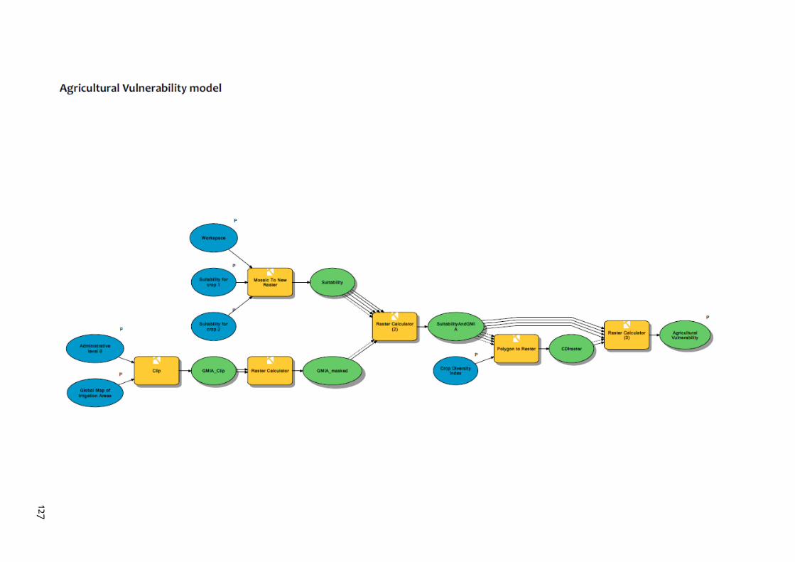
127

Accessibility model
Input
Elevation (GLOBE): raster
LandCover (GlobCover) : raster
Administrative level 0 boundaries (GADM): polygon feature
Market Locations: point feature
Transportation (VMAP0): line feature
Tools
CLIP, CLIP(2), CLIP(3) : Land Cover (global), Elevation (continental tile) and Market
locations (global) are clipped on the administrative level 0 boundaries.
Intermediate outputs: GlobCover_Clip, GLOBE_Clip, Market_Locations_Clip
RECLASSIFY(2): clipped Land Cover (GlobCover_Clip) is reclassified in order to assign
NoData value to certain classes (210 Water bodies, 220 Permanent Snow and ice, 230
NoData)
Intermediate output: GlobCover_REC
JOIN FIELD: a field containing the crossing time for each type of land cover is joined to
the reclassified Land Cover. The GlobCover raster table was previously created with the
Build Raster Attribute Table tool and the crossing time was added in a new field on the
basis of the values reported in (F. Pozzi & Robinson, 2008).
Intermediate output: GlobCover_REC (2)
LOOKUP: it creates a new raster by looking up values of a specific field, in this case it
creates a raster with the value of the just added crossing time field.
Intermediate output: Lookup_GlobCover
RESAMPLE(3): the Elevation raster is resampled to the Land Cover cell size (300 m)
Intermediate output: GLOBE_Resample
PROJECT RASTER: the Elevation raster is transformed in projected coordinates into the
country correspondent UTM coordinate system (WGS84). The operation is needed to
calculate the slope.
Intermediate output: GLOBE_Res_Proj
SLOPE: a slope raster is calculated on the basis of the Elevation raster. Output
measurement is percent rise.
Intermediate output: Slope_output
PROJECT RASTER(2): the slope is transformed again into geographic coordinates.
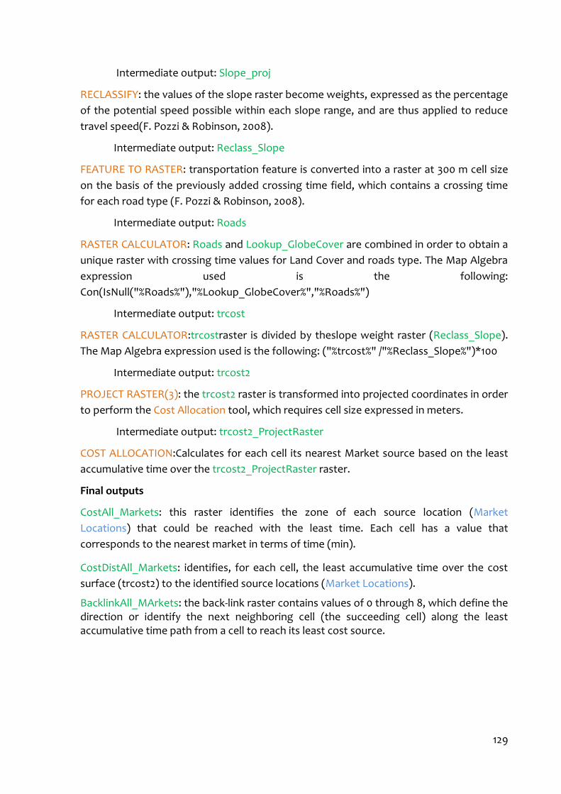
129
Intermediate output: Slope_proj
RECLASSIFY: the values of the slope raster become weights, expressed as the percentage
of the potential speed possible within each slope range, and are thus applied to reduce
travel speed(F. Pozzi & Robinson, 2008).
Intermediate output: Reclass_Slope
FEATURE TO RASTER: transportation feature is converted into a raster at 300 m cell size
on the basis of the previously added crossing time field, which contains a crossing time
for each road type (F. Pozzi & Robinson, 2008).
Intermediate output: Roads
RASTER CALCULATOR: Roads and Lookup_GlobeCover are combined in order to obtain a
unique raster with crossing time values for Land Cover and roads type. The Map Algebra
expression used is the following:
Con(IsNull("%Roads%"),"%Lookup_GlobeCover%","%Roads%")
Intermediate output: trcost
RASTER CALCULATOR:trcostraster is divided by theslope weight raster (Reclass_Slope).
The Map Algebra expression used is the following: ("%trcost%" /"%Reclass_Slope%")*100
Intermediate output: trcost2
PROJECT RASTER(3): the trcost2 raster is transformed into projected coordinates in order
to perform the Cost Allocation tool, which requires cell size expressed in meters.
Intermediate output: trcost2_ProjectRaster
COST ALLOCATION:Calculates for each cell its nearest Market source based on the least
accumulative time over the trcost2_ProjectRaster raster.
Final outputs
CostAll_Markets: this raster identifies the zone of each source location (Market
Locations) that could be reached with the least time. Each cell has a value that
corresponds to the nearest market in terms of time (min).
CostDistAll_Markets: identifies, for each cell, the least accumulative time over the cost
surface (trcost2) to the identified source locations (Market Locations).
BacklinkAll_MArkets: the back-link raster contains values of 0 through 8, which define the direction or identify the next neighboring cell (the succeeding cell) along the least accumulative time path from a cell to reach its least cost source.
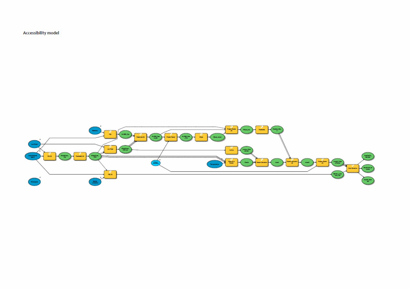
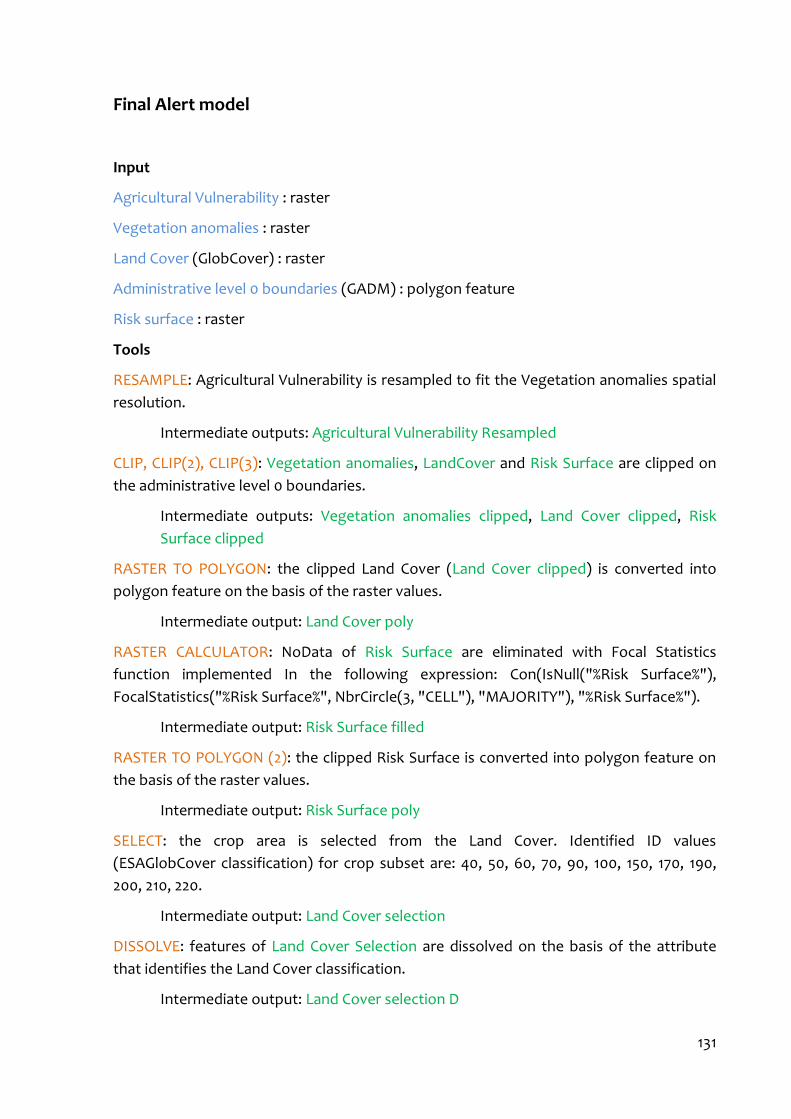
131
Final Alert model
Input
Agricultural Vulnerability : raster
Vegetation anomalies : raster
Land Cover (GlobCover) : raster
Administrative level 0 boundaries (GADM) : polygon feature
Risk surface : raster
Tools
RESAMPLE: Agricultural Vulnerability is resampled to fit the Vegetation anomalies spatial
resolution.
Intermediate outputs: Agricultural Vulnerability Resampled
CLIP, CLIP(2), CLIP(3): Vegetation anomalies, LandCover and Risk Surface are clipped on
the administrative level 0 boundaries.
Intermediate outputs: Vegetation anomalies clipped, Land Cover clipped, Risk
Surface clipped
RASTER TO POLYGON: the clipped Land Cover (Land Cover clipped) is converted into
polygon feature on the basis of the raster values.
Intermediate output: Land Cover poly
RASTER CALCULATOR: NoData of Risk Surface are eliminated with Focal Statistics
function implemented In the following expression: Con(IsNull("%Risk Surface%"),
FocalStatistics("%Risk Surface%", NbrCircle(3, "CELL"), "MAJORITY"), "%Risk Surface%").
Intermediate output: Risk Surface filled
RASTER TO POLYGON (2): the clipped Risk Surface is converted into polygon feature on
the basis of the raster values.
Intermediate output: Risk Surface poly
SELECT: the crop area is selected from the Land Cover. Identified ID values
(ESAGlobCover classification) for crop subset are: 40, 50, 60, 70, 90, 100, 150, 170, 190,
200, 210, 220.
Intermediate output: Land Cover selection
DISSOLVE: features of Land Cover Selection are dissolved on the basis of the attribute
that identifies the Land Cover classification.
Intermediate output: Land Cover selection D
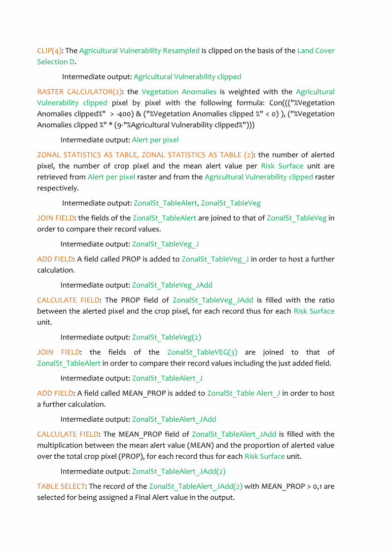
CLIP(4): The Agricultural Vulnerability Resampled is clipped on the basis of the Land Cover
Selection D.
Intermediate output: Agricultural Vulnerability clipped
RASTER CALCULATOR(2): the Vegetation Anomalies is weighted with the Agricultural
Vulnerability clipped pixel by pixel with the following formula: Con((("%Vegetation
Anomalies clipped%" > -400) & ("%Vegetation Anomalies clipped %" < 0) ), ("%Vegetation
Anomalies clipped %" * (9-"%Agricultural Vulnerability clipped%")))
Intermediate output: Alert per pixel
ZONAL STATISTICS AS TABLE, ZONAL STATISTICS AS TABLE (2): the number of alerted
pixel, the number of crop pixel and the mean alert value per Risk Surface unit are
retrieved from Alert per pixel raster and from the Agricultural Vulnerability clipped raster
respectively.
Intermediate output: ZonalSt_TableAlert, ZonalSt_TableVeg
JOIN FIELD: the fields of the ZonalSt_TableAlert are joined to that of ZonalSt_TableVeg in
order to compare their record values.
Intermediate output: ZonalSt_TableVeg_J
ADD FIELD: A field called PROP is added to ZonalSt_TableVeg_J in order to host a further
calculation.
Intermediate output: ZonalSt_TableVeg_JAdd
CALCULATE FIELD: The PROP field of ZonalSt_TableVeg_JAdd is filled with the ratio
between the alerted pixel and the crop pixel, for each record thus for each Risk Surface
unit.
Intermediate output: ZonalSt_TableVeg(2)
JOIN FIELD: the fields of the ZonalSt_TableVEG(3) are joined to that of
ZonalSt_TableAlert in order to compare their record values including the just added field.
Intermediate output: ZonalSt_TableAlert_J
ADD FIELD: A field called MEAN_PROP is added to ZonalSt_Table Alert_J in order to host
a further calculation.
Intermediate output: ZonalSt_TableAlert_JAdd
CALCULATE FIELD: The MEAN_PROP field of ZonalSt_TableAlert_JAdd is filled with the
multiplication between the mean alert value (MEAN) and the proportion of alerted value
over the total crop pixel (PROP), for each record thus for each Risk Surface unit.
Intermediate output: ZonalSt_TableAlert_JAdd(2)
TABLE SELECT: The record of the ZonalSt_TableAlert_JAdd(2) with MEAN_PROP > 0,1 are
selected for being assigned a Final Alert value in the output.

133
Intermediate output: ZonalSt_TableAlert_Sel
JOIN FIELD (2): The MEAN_PROP field of ZonalSt_TableAlert_Sel is joined to the Risk
Surface poly.
Final outputs
Final Alert: this polygon feature identifies and shows, through appropriate symbology,
the final alert values given per Risk Surface unit.


135
Huff step 1 model
Input
Sorted markets : point layer
Cost raster projected : raster
Tools
ITERATE FEATURE SELECTION: Iterates over features of a layer returning one record at a
time that is used for further processing and a number (Value) which is the identifier of the
record being used.
Intermediate outputs: I Sorted Markets
COST DISTANCE: For each of the Sorted Markets the cost distance is calculated taking
into account the only market being used and the Cost Raster calculated with the
Accessibility model and being reprojected into a suitable projected coordinate reference
system.
Intermediate outputs: Cost Distance Gravity
GET FIELD VALUE: This tool returns, per record being used, the value of the Influence field
of the Sorted Markets attribute table.
Intermediate outputs: Influence field value
RASTER CALCULATOR: Multiplies each of the pixel of the Cost Distance Gravity raster per
the correspondent Influence value.
Final outputs
Utility%Value%: The raster contains the utility values for a specific market. This model
returns as output as many Utility rasters as the number of records of the Sorted markets
layer. Each of the output rasters is identified with the number stored in Value returned by
the ITERATE FEATURE SELECTION tool.
Huff step 2 model
Input
Utility : rasters
Tools
RASTER CALCULATOR: Calculates the summation of all the Utility rasters provided in
input.
Intermediate outputs: Summation
ITERATE RASTER: Given the workspace in which the Utility rasters are stored, this tool
iterates over the rasters and returns one raster per iteration and its Name.
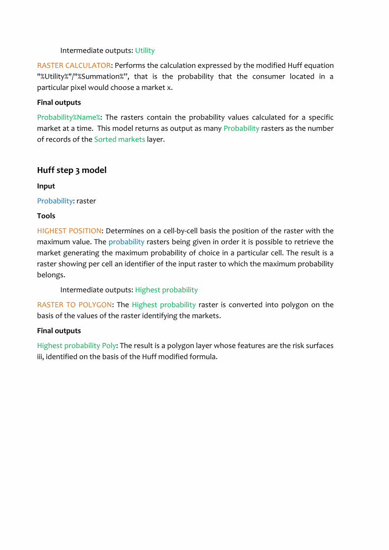
Intermediate outputs: Utility
RASTER CALCULATOR: Performs the calculation expressed by the modified Huff equation
"%Utility%"/"%Summation%”, that is the probability that the consumer located in a
particular pixel would choose a market x.
Final outputs
Probability%Name%: The rasters contain the probability values calculated for a specific
market at a time. This model returns as output as many Probability rasters as the number
of records of the Sorted markets layer.
Huff step 3 model
Input
Probability: raster
Tools
HIGHEST POSITION: Determines on a cell-by-cell basis the position of the raster with the
maximum value. The probability rasters being given in order it is possible to retrieve the
market generating the maximum probability of choice in a particular cell. The result is a
raster showing per cell an identifier of the input raster to which the maximum probability
belongs.
Intermediate outputs: Highest probability
RASTER TO POLYGON: The Highest probability raster is converted into polygon on the
basis of the values of the raster identifying the markets.
Final outputs
Highest probability Poly: The result is a polygon layer whose features are the risk surfaces
iii, identified on the basis of the Huff modified formula.
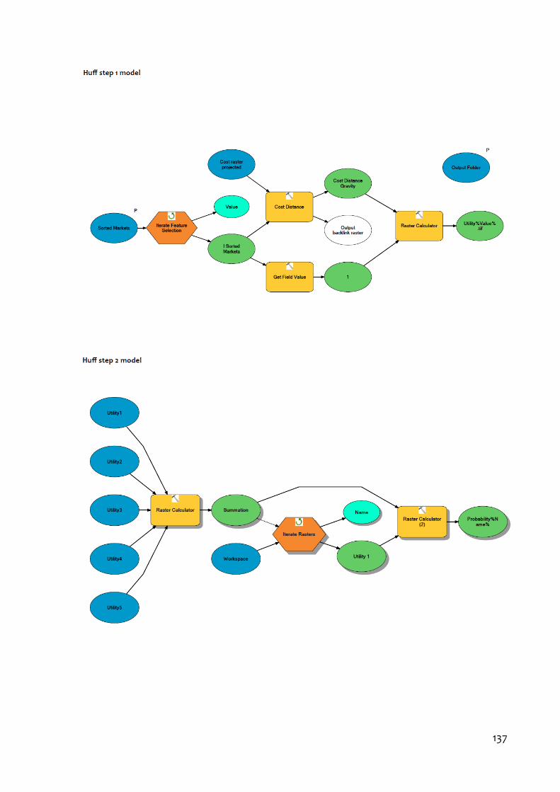
137
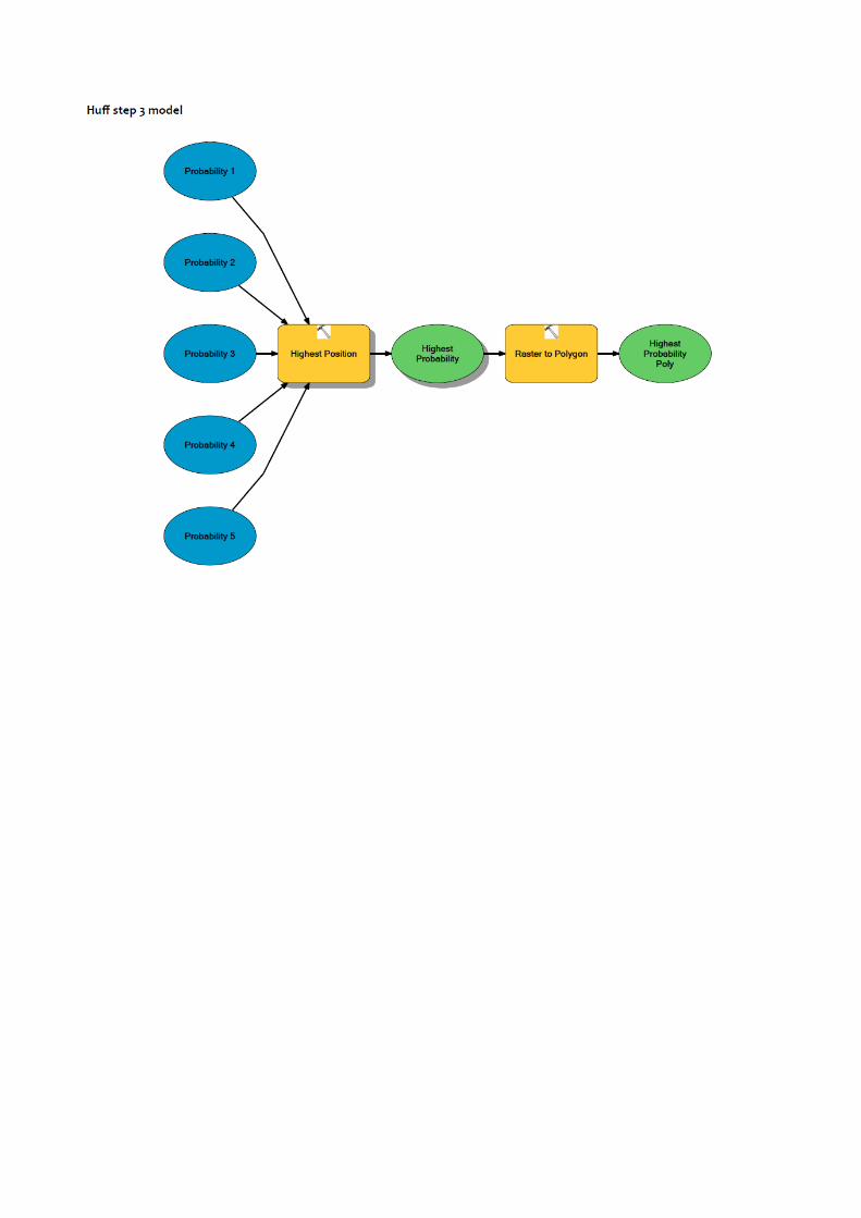

139
BIBLIOGRAPHY
Adger, N. W., Arnell, N. W., & Tompkins, E. L. (2005). Successful adaptation to climate change across scales. Global Environmental Change, 15(2), 77–86. doi:10.1016/j.gloenvcha.2004.12.005
Adger, W. N. (2000). Social and ecological resilience: are they related? Progress in Human Geography, 24(3), 347–364. doi:10.1191/030913200701540465
Adger, W. N. (2006). Vulnerability. Global Environmental Change, 16(3), 268–281. doi:10.1016/j.gloenvcha.2006.02.006
Allenby, B., & Fink, J. (2005). Toward inherently secure and resilient societies. Science (New York, N.Y.), 309(5737), 1034–6. doi:10.1126/science.1111534
Angeluccetti, I., & Perez, F. (2013). Drought hazard assessment and vulnerability mapping. In The Value of Geoinformation for Disaster and Risk Management (VALID). Benefit Analysis and Stakeholder Assessment. (pp. 54–61). Copenhagen, Denmark: Joint Board of Geospatial Information Societies (JB GIS).
Applebaum, W., & Cohen, S. B. (1961). The Dynamics of Store Trading Areas and Market Equilibrium. Annals of the Association of the American Geographer, 51, 73–101.
Bailey, R. (2013). Managing Famine Risk Linking Early Warning to Early Action. London. Retrieved from http://www.chathamhouse.org/sites/default/files/public/Research/Energy, Environment and Development/0413r_earlywarnings.pdf
Barrett, C. B. (2010). Measuring food insecurity. Science (New York, N.Y.), 327(5967), 825–8. doi:10.1126/science.1182768
Beekhuis, G., & Laouali, I. (2007). Cross-border trade and food markets in Niger: why market analysis is important for humanitarian action. Humanitarian Practice Network, 44(38), 25–38.
Bellone, T., Boccardo, P., & Perez, F. (2009). Investigation of Vegetation Dynamics using Long-Term Normalized Difference Vegetation Index Time-Series. American Journal of Environmental Sciences, 5(4), 461–467.
Below, R., Grover-Kopec, E., & Dilley, M. (2007). Documenting Drought-Related Disasters: A Global Reassessment. The Journal of Environment & Development, 16(3), 328–344. doi:10.1177/1070496507306222
Bernus, E., Hamidou, S. A., & Laclavère, G. (1980). Atlas du Niger (Jeune Afri.).
Birkmann, J. (2006a). Indicators and criteria for measuring vulnerability: Theoretical bases and requirements. In J. Birkmann (Ed.), Measuring vulnerability to natural hazards:

towards disaster resilient societies (Vol. 02, pp. 55–77). United Nations University Press.
Birkmann, J. (2006b). Measuring vulnerability to promote disaster-resilient societies : Conceptual frameworks and definitions (Vol. 01, pp. 9–54).
Birkmann, J., & Mucke, P. (2011). World Risk Report.
Boccardo, P., Perez, F., Giulio Tonolo, F., Pasquali, P., Steffenino, S., Facello, A., … Angeluccetti, I. (2012). Call for tenders No ENTR/2009/27 Lot 2 - Implementation of an initial GMES service for geospatial reference data access covering areas outside Europe. D10.1 - D10.2 - D10.3 - Task 10 Analysis of non-European reference data availability (M30). Torino.
Bogardi, J. J., & Birkmann, J. (2004). Vulnerability assessment: the first step towards sustainable risk reduction. In D. Malzahn & T. Plapp (Eds.), Disasters and society. From Hazard Assessment to Risk Reduction. Berlin, DE: Logos Verlag.
Bohle, H. G., Downing, T. E., & Michael, J. (1994). Climate change and social vulnerability. Toward a sociology and geography of food insecurity. Global Environmental Change, 4(1), 37–48.
Bryant, E. (1991). Natural hazards (p. 294 + XVII). Cambridge, UK: Cambridge University Press.
Bryant, E. (2005). Natural hazards (2nd ed., p. 328). Cambridge, UK: Cambridge University Press.
Cabinet du Premier Ministre du Niger - DNPGCCA. (2013). Plan de soutien Préliminaire aux populations vulnérables (p. 44). Niamey.
Cannon, T., Twigg, J., & Rowell, J. (2003). Social vulnerability, sustainable livelihoods and disasters.
Chasco Yrigoyen, C., & Vicéns Otero, J. (1998). SPATIAL INTERACTION MODELS APPLIED TO THE DESIGN OF RETAIL TRADE AREAS.
Christaller, W. (1933). Die zentralen Orte in Süddeutschland. Jena: Fischer G.
Cicone, R. C., Parris, T. M., Way, D. S., & Chiesa, C. (2003). Geospatial Modeling to Identify Populations Vulnerable to Natural Hazards. In International Symposium on Remote Sensing of Environment. Honolulu.
Collinet, J., & Valentin, C. (1984). Evaluation of factors influencing water erosion in West Africa using rainfall simulation.
Cutter, S. L. (1996). Vulnerability to environmental hazards. Progress in Human Geography, 20(4), 529–539.
141
Cutter, S. L., Boruff, B. J., & Shirley, W. L. (2003). Social vulnerability to environmental hazards. Social Science Quarterly, 84(2), 242–261.
Dai, A. (2011). Drought under global warming: a review. Wiley Interdisciplinary Reviews: Climate Change, 2(1), 45–65. doi:10.1002/wcc.81
De Waal, A. (1989). Famine that kills: Darfur, Sudan, 1984–5. Oxford, UK: Oxford University Press, Inc.
Downing, T. (2004). “‘What Have We Learned Regarding a Vulnerability Science?’” In Science in Support of Adaptation to Climate Change. Side Event of the 10th Session of the Conference of the Parties to the United Nations Framework Convention on Climate Change (pp. 18–21). Buenos Aires.
Downing, T. E., Aerts, J., Soussan, J., Barthelemy, O., Bharwani, S., Ionescu, C., … Ziervogel, G. (2006). INTEGRATING SOCIAL VULNERABILITY INTO WATER MANAGEMENT. Oxford, UK.
Dracup, J. a., Lee, K. S., & Paulson, E. G. (1980). On the definition of droughts. Water Resources Research, 16(2), 297–302. doi:10.1029/WR016i002p00297
Economic Commission for Latin America and the Caribbean & the World Bank. (2003). Handbook for estimating the socio-economic and environmental effects of disasters. Volume I. Washington, DC, USA.
Eriyagama, N., Smakhtin, V., & Gamage, N. (2010). A global picture of drought occurrence , magnitude and preparedness. Options Méditerranéennes, 95, 19–25.
Eriygama, N., Smakhtin, V., & Gamage, N. (2009). Mapping Drought Patterns and Impacts: A Global Perspective.
FAO. (2008). Markets Assessment and Analysis - Lesson 1 - Markets and Food Security. Notes.
FAO. (2013). FAO Statistical Yearbook 2013 World food and agriculture. Rome, IT.
FAO Subregional Office for Southern and East Africa Harare. (2004). Drought impact mitigation and prevention in the Limpopo River Basin. Rome, IT.
Federal Emergency Management Agency. (1995). National mitigation strategy; Partnerships for building safer communities. Washington, DC, USA.
Fotheringam, A. S., & O’Kelly, M. E. (1989). Spatial Interaction Models: Formulations and Applications. Boston: Kluwer Academic Publishers.
Garrote, L. (2012). Methodology for definition of drought vulnerability across Africa.
Geesing, D., & Djibo, H. (2006). Country Pasture / Forage Resource Profiles NIGER (p. 24). Rome, IT.

Glantz, M. H. (1987). Drought and hunger in Africa: Denying Famine a Future. Cambridge, UK: Cambridge University Press.
Goodall, B. (1987). A Dictionary of Modern Human Geography. (Penguin Bo.). England.
Grillo, J. (2009). Application of the Livelihood Zone Maps and Profiles for Food Security Analysis and Early Warning.
Hahn, M. B., Riederer, A. M., & Foster, S. O. (2009). The Livelihood Vulnerability Index: A pragmatic approach to assessing risks from climate variability and change—A case study in Mozambique. Global Environmental Change, 19(1), 74–88. doi:10.1016/j.gloenvcha.2008.11.002
Heim, R. (2002). A rievew of Twentieth-Century Drought Indices Used in the United States. Direct, (August), 1149–1165.
Hewitt, K. (1997). Regions at Risk: A Geographical Introduction to Disasters. Longman, UK: Addison-Wesley.
Hillbruner, C. (2012). Scenario Development for Food Security Early Warning Guidance for Famine Early Warning Systems Network Staff and Partners.
Hillbruner, C., & Moloney, G. (2012). When early warning is not enough—Lessons learned from the 2011 Somalia Famine. Global Food Security, 1(1), 20–28. doi:10.1016/j.gfs.2012.08.001
Huff, D. L. (1962). A Probabilistic Analysis of Consumer Spatial Behaviour. In Emerging Concepts in Marketing. Pittsburgh: American Marketing Association.
International Federation of Red Cross and Red Crescent Societies. (2006). Eastern Africa: Regional drought response (DREF Bulletin No. MDR64001).
International Research Institute for Climate and Society. (2005). Sustainable development in Africa: Is the climate right? (IRI Technical Report Number IRI-TR/05/1). Palisades, New York.
IPC Global Partners. (2012). Integrated Food Security Phase Classification Technical Manual Version 2.0. Evidence and Standards for Better Food Security Decisions. Rome: FAO.
Jones, K. J., & Mock, D. R. (1984). Store Location and Assessment Research. (R. L. Davies & D. S. Rogers, Eds.)Store Location and Store Assessment Research. New York: John Wiley.
Julich, S. (2006). Drought risk indicators for assessing rural households. In Summer Academy on Social Vulnerability. Hohenkammer: Munich Re foundation; UNU-EHS.
Løvendal, C. R., & Knowles, M. (2004). Understanding Vulnerability to Food Insecurity Lessons from Vulnerable Livelihood Profiling.
143
Luce, R. (1959). Individual Choice Behaviour. New York: John Wiley.
Miller, J. B., Cunningham, D., Koeln, G., Way, D., Metzler, J., & Cicone, R. (2002). GLOBAL DATABASE FOR GEOSPATIAL INDICATORS. In Pecora 15/Land Satellite Information IV/ISPRS Commission I/FIEOS.
Minamiguchi, N. (2005). The Application of Geospatial and Disaster Information for Food Insecurity and Agricultural Drought Monitoring and Assessment by the FAO GIEWS and Asia FIVIMS. In Workshop on Reducing Food Insecurity Associated with Natural Disasters in Asia and the Pacific.
Mishra, A. K., & Singh, V. P. (2010). A review of drought concepts. Journal of Hydrology, 391(1-2), 202–216. doi:10.1016/j.jhydrol.2010.07.012
Mitchell, D. (2008). A Note on Rising Food Prices. Retrieved from http://www-wds.worldbank.org/external/default/WDSContentServer/IW3P/IB/2008/07/28/000020439_20080728103002/Rendered/PDF/WP4682.pdf
Nyabeze, W. (2012). Inventory of institutional frameworks and drought mitigation and adaptation practices in Africa.
Obasi, G. O. P. (1994). WMO’s role in the International Decade for Natural Disaster Reduction. Bulletin of the American Meteorological Society, 75(9), 1655–1661. doi:10.1175/1520-0477
Peduzzi, P., Dao, H., Herold, C., & Mouton, F. (2009). Assessing global exposure and vulnerability towards natural hazards: the Disaster Risk Index. Natural Hazards and Earth System Science, 9(4), 1149–1159. doi:10.5194/nhess-9-1149-2009
Pozzi, F., & Robinson, T. (2008). Accessibility Mapping in the Horn of Africa : Applications for Livestock Policy.
Pozzi, F., Robinson, T., & Nelson, A. (2010). Accessibility Mapping and Rural Poverty in the Horn of Africa.
Pozzi, W., Cripe, D., Heim, R., Brewer, M. J., & Sheffield, J. (2011). Group on Earth Observation (GEO) Global Drought Monitor. In EGU 2011 (Vol. 13).
Pozzi, W., Sheffield, J., Stefanski, R., Cripe, D., Pulwarty, R., Vogt, J., … Lawford, R. (2013). TOWARD GLOBAL DROUGHT EARLY WARNING CAPABILITY: Expanding International Cooperation for the Development of a Framework for Monitoring and Forecasting. Bulletin of the American Meteorological Society, 94(6), 776–785.
Redmond, K. T. (2002). The depiction of drought. Bullettin of the American Meteorological Society, (August), 1143–1147.
Reilly, W. J. (1931). The Law of Retail Gravitation. New York: Reilly, W.J.

Roose, E. (1977). Erosion et ruissellemet en Afrique de l’Ouest. Vingt années de mesures en petites parcelles expérimentales.
Rust, R. T., & Donthu, N. (1995). Capturing Geographically Localized Misspecification Error in Retail Store Choice Models. Journal of Marketing Research, 32(1), 103–110.
Sanogo, I. (n.d.). Market Analysis Tool How to Conduct a Trader Survey ?
Sen, A. (1981). Poverty and Famines: An Essay on Entitlement and Deprivation. Oxford, UK: Clarendon Press.
Siebert, S., Henrich, V., Karen, F., & Burke, J. (2013). Global Map of Irrigation Areas version 5. Rome, IT.
Slim, H. (2012). Real-Time Evaluation of the Humanitarian Response to the Horn of Africa Drought Crisis in Somalia, Ethiopia and Kenya - Synthesis report.
SWAC/OECD. (2013). AGIR – SAHEL AND REGIONAL ROADMAP (p. 28). Paris (FR). Retrieved from http://www.oecd.org/swac/publications/AGIR roadmap_EN_FINAL.pdf
Tracey-White, J. (1999). Market Infrastructure Planning - A guide for decision makers. Rome, IT.
Tschirley, D., Nijhoff, J. J., Arlindo, P., Mwinga, B., Weber, M. T., & Jayne, T. (2004). Anticipating and Responding to Drought Emergencies in Southern Africa: Lessons from the 2002-2003 Experience.
UN. (2006). Global Survey of Early Warning Systems. Geneva, Switzerland.
UN/ISDR. (2004a). Living with Risk - Volume I (UN., Vol. I). Geneva, Switzerland.
UN/ISDR. (2004b). Living with Risk - Volume II (UN., Vol. II). Geneva, Switzerland.
UN/ISDR. (2005). WCDR - Hyogo Framework for Action 2005-2015. Building the Resilience of Nations and Communities to Disasters. Kobe, Hyogo, Japan.
UN/ISDR. (2009). Drought Risk Reduction Framework and Practices (p. 213). Geneva, Switzerland: UN/ISDR.
UNDP. (2004). Reducing disaster risk: A challenge for development. New York.
UNEP. (2012). Early Warning Systems: A State of the Art Analysis and Future Directions. (V. F. Grasso & A. Singh, Eds.). Nairobi. Retrieved from http://www.unep.org
Vogel, C., & O’Brien, K. (2004). Vulnerability and Global Environmental Change: Rhetoric and Reality. Retrieved from http://www.gechs.org/ publications/aviso/13/index.html

145
Webb, P., Coates, J., Frongillo, E. A., Rogers, L., Swindale, A., & Bilinsky, P. (2006). Measuring Household Food Insecurity : Why It’s So Important and Yet So Difficult to Do. Journal of Nutrition, (2), 1404–1408.
WFP. (2009). Emergency Food Security Assessment Handbook (Second.). Rome, IT.
Wilcox, R., Kassam, F., Syroka, J., & Cousins, B. (n.d.). Africa RiskView.
Wilhite, D. A. (1999). Drought preparedness in the Sub-Saharan Africa Context. In Integrated Drought Management: Lessons for sub Saharan Africa. Pretoria.
Wilhite, D. A., & Glantz, M. H. (1985). Understanding the drought phenomenon: the role of definitions. Water International, 10(3), 111–120. doi:10.1080/02508068508686328
Yevjevich, V. (1967). AN OBJECTIVE APPROACH TO DEFINITIONS AND INVESTIGATIONS OF CONTINENTAL HYDROLOGIC DROUGHTS. Fort Collins, Colorado.