Embed Size (px)
Citation preview
POLITECNICO DI MILANO
Facoltà di Ingegneria dell’Informazione
Corso di Laurea Magistrale in Ingegneria Informatica
Ontology-assisted approach for learning
causal Bayesian network structure
Relatore: Prof.ssa Giuseppina Gini
Tesi di Laurea di:
Denis ĆUTIĆ
Matricola n. 764725
Anno Accademico 2012-2013

To my family
i
Contents 1 Introduction .............................................................................................................................. 1
1.1 Motivation ......................................................................................................................... 1
1.2 Outline ............................................................................................................................... 2
2 Background ............................................................................................................................... 3
2.1 Bayesian networks ............................................................................................................. 3
2.1.1 Introduction ................................................................................................................ 3
2.1.2 Causality ..................................................................................................................... 6
2.1.3 Causal structure learning ........................................................................................... 8
2.1.4 State of the art algorithms ....................................................................................... 10
2.2 Ontology .......................................................................................................................... 18
2.2.1 Introduction .............................................................................................................. 18
2.2.2 Causal relationships.................................................................................................. 18
2.2.3 Reasoning ................................................................................................................. 21
3 Related work .......................................................................................................................... 24
4 The algorithm ......................................................................................................................... 27
4.1 Steps of the algorithm ..................................................................................................... 28
4.1.1 Data preparation ...................................................................................................... 28
4.1.2 Structure learning with PC algorithm ....................................................................... 29
4.1.3 Node annotation ...................................................................................................... 30
4.1.4 Inferring undirected edge orientation from the ontology ....................................... 32
4.2 Complexity analysis ......................................................................................................... 33
4.2.1 PC algorithm complexity .......................................................................................... 34
4.2.2 Ontology inference complexity ................................................................................ 35
5 Example .................................................................................................................................. 37
5.1 Resources ......................................................................................................................... 37
5.1.1 Yeast cell cycle dataset ............................................................................................. 37
5.1.2 Gene Ontology ......................................................................................................... 38
5.1.3 Annotations .............................................................................................................. 39
ii
5.2 Results .............................................................................................................................. 40
5.2.1 Algorithm performance ............................................................................................ 41
5.2.2 Comparison to other approaches ............................................................................ 45
5.3 Discussion ........................................................................................................................ 48
6 Conclusion .............................................................................................................................. 50
7 Appendix ................................................................................................................................. 51
7.1 Relation properties .......................................................................................................... 51
7.2 Ontology inference step code ......................................................................................... 51
7.3 Evidence codes ................................................................................................................ 53
7.4 Class diagrams ................................................................................................................. 55
8 Bibliography ............................................................................................................................ 57
9 Internet resources .................................................................................................................. 61
iii
List of Figures
Figure 1 – A simple causal network .................................................................................................. 8
Figure 2 – An example ontology ..................................................................................................... 20
Figure 3 - PC algorithm ................................................................................................................... 31
Figure 4 – PC algorithm rules ......................................................................................................... 31
Figure 5 - Ontology fragment ......................................................................................................... 43
Figure 6 - YGL021W (ALK1) interaction network ........................................................................... 44
Figure 7 - YCR040W (MATALPHA1) and YCL066W (HMLAPHA1) interaction networks ................ 45

iv
List of Tables
Table 1 – YGR108W and YGL021W annotations ............................................................................ 42
Table 2 - Number of edges found................................................................................................... 47
Table 3 - Constraint-based algorithms ........................................................................................... 47
Table 4 - Score-based algorithms ................................................................................................... 48
v
Abstract
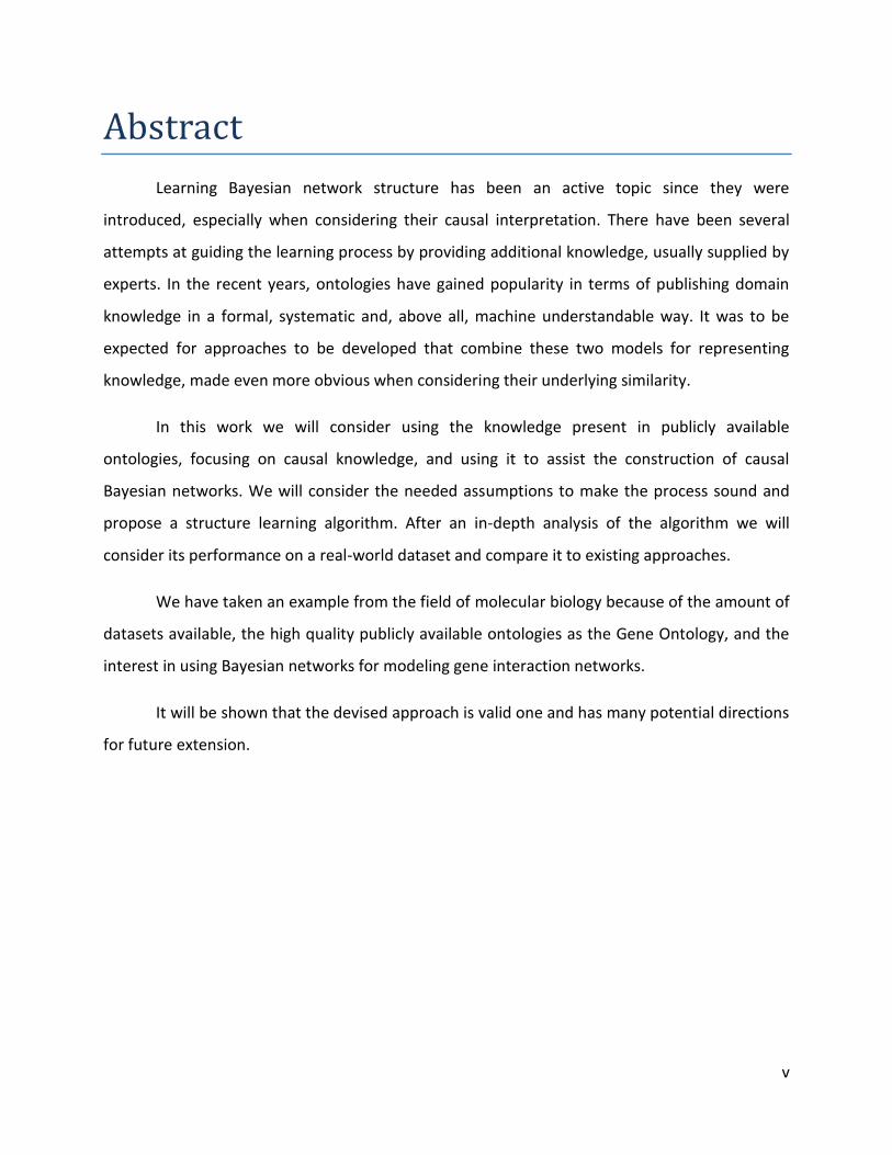
Learning Bayesian network structure has been an active topic since they were
introduced, especially when considering their causal interpretation. There have been several
attempts at guiding the learning process by providing additional knowledge, usually supplied by
experts. In the recent years, ontologies have gained popularity in terms of publishing domain
knowledge in a formal, systematic and, above all, machine understandable way. It was to be
expected for approaches to be developed that combine these two models for representing
knowledge, made even more obvious when considering their underlying similarity.
In this work we will consider using the knowledge present in publicly available
ontologies, focusing on causal knowledge, and using it to assist the construction of causal
Bayesian networks. We will consider the needed assumptions to make the process sound and
propose a structure learning algorithm. After an in-depth analysis of the algorithm we will
consider its performance on a real-world dataset and compare it to existing approaches.
We have taken an example from the field of molecular biology because of the amount of
datasets available, the high quality publicly available ontologies as the Gene Ontology, and the
interest in using Bayesian networks for modeling gene interaction networks.
It will be shown that the devised approach is valid one and has many potential directions
for future extension.
vi
Sommario
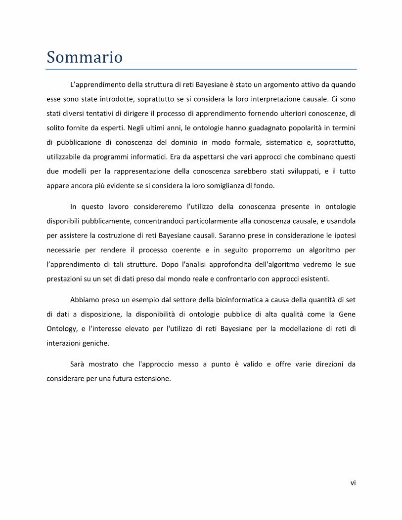
L’apprendimento della struttura di reti Bayesiane è stato un argomento attivo da quando
esse sono state introdotte, soprattutto se si considera la loro interpretazione causale. Ci sono
stati diversi tentativi di dirigere il processo di apprendimento fornendo ulteriori conoscenze, di
solito fornite da esperti. Negli ultimi anni, le ontologie hanno guadagnato popolarità in termini
di pubblicazione di conoscenza del dominio in modo formale, sistematico e, soprattutto,
utilizzabile da programmi informatici. Era da aspettarsi che vari approcci che combinano questi
due modelli per la rappresentazione della conoscenza sarebbero stati sviluppati, e il tutto
appare ancora più evidente se si considera la loro somiglianza di fondo.
In questo lavoro considereremo l’utilizzo della conoscenza presente in ontologie
disponibili pubblicamente, concentrandoci particolarmente alla conoscenza causale, e usandola
per assistere la costruzione di reti Bayesiane causali. Saranno prese in considerazione le ipotesi
necessarie per rendere il processo coerente e in seguito proporremo un algoritmo per
l’apprendimento di tali strutture. Dopo l'analisi approfondita dell'algoritmo vedremo le sue
prestazioni su un set di dati preso dal mondo reale e confrontarlo con approcci esistenti.
Abbiamo preso un esempio dal settore della bioinformatica a causa della quantità di set
di dati a disposizione, la disponibilità di ontologie pubblice di alta qualità come la Gene
Ontology, e l'interesse elevato per l'utilizzo di reti Bayesiane per la modellazione di reti di
interazioni geniche.
Sarà mostrato che l'approccio messo a punto è valido e offre varie direzioni da
considerare per una futura estensione.
1
1 Introduction
1.1 Motivation
The popularity of Bayesian networks for representing uncertain knowledge, and
ontologies for storing machine readable and structured knowledge has made people consider
combined approaches. The main motivation to consider such an approach is made obvious
when realizing the high similarity of their underlying structures. This similarity allows for
knowledge to be transferred both ways, and thus two main approaches have been considered.
One line of thought tries to incorporate uncertainty into ontologies, while the other wants to
exploit the knowledge present in them to guide the construction of the Bayesian network
structure. Our approach will follow the latter one. Moreover, we will consider our Bayesian
network to have a causal interpretation and will be interested solely in its structure,
disregarding the form of the causal relations.
General interest in the causal interpretation of the Bayesian networks is due to the
stability of its relations. Once we know there exist a causal relation between two variables we
know it to be an objective and physical constraint in our world. This comes at a price, the task of
finding and justifying such a relation has proven to be quite non-trivial, especially when the goal
is to learn them from offline data. In that case, even under reasonable assumptions, which may
not hold in general, the process is driven by covariation and does not give us the guarantee of
causality.
On the other hand we can expect ontologies to comprise in themselves among others,
also causal knowledge. This is exactly the knowledge we want to exploit and for which we
believe that reflects the true state of the world for the give domain.
Following the discussion above, we can formulate the main idea behind our approach.
We will be considering using publicly available domain knowledge in form of ontologies to assist
the learning process of causal network structures. We say “assist” because the approach is
based around a standard structure learning algorithm which uses the ontology for tuning up its

2
results. This general outline of the approach leaves enough space for considering different
points of interaction between the ontology knowledge and the structure learning algorithm.
1.2 Outline
This work is structured as follows. In section 2 we will start by introducing Bayesian
networks, their causal interpretation and looking at both the general idea of structure learning
and at real approaches and their building blocks. Next, in the same section, we will introduce
the concept of ontologies and look at how can they be used for learning causal network
structures. We will continue by looking at the reasoning process for inferring implicit knowledge
present in the ontology, and focusing on the one needed for our application. Before venturing
into a deeper analysis of our approach, in section 3, we will take a look at some similar
approaches taken by various groups. Later, in section 4, we will deal with the analysis of our
approach with a detailed consideration of each algorithm step and end by considering its
computational complexity. In section 5, we will look at the performance of our approach on a
real world example from the molecular biology domain, compare it to other approaches and
discuss the results. To conclude, in section 6, we are going to consider the open issues and
possible extensions of this work.
3
2 Background
2.1 Bayesian networks
2.1.1 Introduction
Bayesian networks, also called belief networks, probabilistic networks, or causal
networks, were developed to facilitate the task of prediction and abduction1 in artificial
intelligence systems. In these tasks, it is necessary to find a coherent interpretation of incoming
observations that is consistent with both the observations and the prior information at hand.
Mathematically, the task boils down to the computation of , where is a set of
observations and is a set of variables that are deemed important for prediction or diagnosis.
The computation involves a straightforward application of the Bayes’ rule [39].
Formally, Bayesian networks are directed acyclic graphs (DAGs) composed of nodes,
which correspond to random variables, and directed edges between nodes, which indicate a
direct influence of the source (parent) node to the target (child) node.
The set of nodes and the set of edges together define the structure of the Bayesian
network . The structure of the network specifies the conditional independence
relationships that hold in the domain being modeled. Thus, inference over a large number of
variables can be decomposed into a set of local calculations involving a small number of
variables. Where conditional independence is defined as follows: given variables or sets of
variables , and we say that and are conditionally independent given if
which can be also written as
Along with the structure, to fully specify a Bayesian network we need to know the
conditionally probability distributions for each random variable , which
1 Abduction is a form of logical inference that goes from observation to a hypothesis that accounts for the reliable
data (observation) and seeks to explain relevant evidence.
4
are the parameters of the model. Whereas the structure defines the parents for each
variable the parameters define the degree of influence in a quantitative way.
Variables can be either discrete or continuous2. In the case of discrete variables for each
variable and its parents we can represent its distribution as a conditional probability
table (CPT). If we take to be the number of possible values of variables
respectively, the CPT for variable will have ∏ entries. This representation can describe
any discrete conditional distribution, but having the downside that the number of free
parameters is exponential in the number of parents.
For continuous variables, unlike the case of discrete variables, there is no representation
that can represent all possible densities. A natural choice for multivariate continuous
distributions is to use Gaussian distributions in the form of linear Gaussian conditional densities,
according to which the conditional density for given its parents is:
( ∑
)
Thus, is normally distributed around a mean that depends linearly on the values of its
parents, and a variance independent of the parents’ values. If all the variables have a linear
Gaussian distribution the joint distribution is a multivariate Gaussian [16].
Markov equivalence
The notion of Markov equivalence will be needed once we start talking about structure
learning algorithms, for which we will need the notion of equivalence classes.
When considering conditional independences, represented in the network structure by
means of directed edges, we are not interested in the edge orientation. The graphs and
both imply the same set of conditional independencies. Therefore, more than one graph
can imply the exact same set of independencies even though their structures differ in the
2 In this work only networks having all variables of the same kind will be considered.

5
orientation of some edges. We say for such graphs to be Markov equivalent and the set of all
equivalent graphs forms an equivalence class. The Markov equivalence is formally defined in the
following theorem.
Theorem: Two DAGs are Markov equivalent if and only if they have the same underlying
undirected graph and the same v-structures (i.e., converging directed edges into the same
nodes, such that , and there is no edge between and ). [16]
An equivalence class can be uniquely represented by a partially directed acyclic graph
(PDAG), where a directed edge means that all the graphs in the class contain it. On the other
hand an undirected edge denotes that graphs in the class disagree on its directionality.
d-separation
We are going to introduce the concept of d-separation since we are going to need it in a
later section, when considering the structure learning algorithm. The intuition behind the
concept is simple and can best be recognized if we attribute causal meaning to the arrows in the
graph. In causal chains and causal forks , the and variables are
marginally independent but become dependent once we condition on the variable.
Figuratively, conditioning on appears to “block” the flow of information along the path, since
learning about has no effect on the probability of given .
Inverted forks , representing two causes having a common effect, act the
opposite way; if the and variables are marginally independent, they will become dependent
once we condition on the variable or any of its descendants.
Formally, we write:
Definition: A path is said to be d-separated (or blocked) by a set of nodes if and only
if:
1. contains a chain or a fork such that the middle node z is in or,
2. contains an inverted fork (or collider) such that the middle node z is not in
and such that no descendant of is in .
6
A set is said to d-separate from if and only if blocks every path from a node in to a
node in .
2.1.2 Causality
A long tradition in psychology and philosophy has investigated the principles of causal
understanding. We understand causation to be a relation between events in which the presence
of some events causes the presence of others [20]. We assume causation to be a causal binary
relation with the properties of being transitive, irreflexive, and asymmetric. That is:
1. if A is a cause of B and B is a cause of C, then A is also a cause of C,
2. an event A cannot cause itself, and
3. if A is a cause of B then B is not a cause of A.
Relative to the set of events causation can be direct or indirect. When we have two events of
which one is the immediate cause of the other we say causation is direct. On the other hand
when there is a chain of causally connected events for which A is the immediate cause and C the
immediate effect then A and C are said to be in an indirect causal relationship. In such a
relationship once it is known that an event has happened it screens off the events that are its
direct and indirect causes from its direct and indirect effects to which we refer as the causal
Markov assumption. By means of causal relationships we can construct a causal network
representing some causal process in the world [39].
If willing to accept the causal Markov assumption we can interpret causal networks as
Bayesian networks which are usually regarded as causal Bayesian networks (CBNs). When the
assumption holds, the causal network satisfies the Markov independencies of the corresponding
Bayesian network. One of the main differences between them is a stricter interpretation on the
meaning of edges for the causal network: direct causal relationships, with parent nodes being
causes, and child nodes effects. There is also a different interpretation of the conditional
distributions which get interpreted as functional relationships between variables.
Moving from a probabilistic model to a causal one we get a model that is much more
informative. While the joint distribution tells us how probable events are and how probabilities
7
with subsequent observations change, a causal model also tells us how these probabilities
would change as a result of external interventions. By means of interventions it is possible to
test whether variable causally influences variable . To do so we compute the marginal
distribution of under the action , namely 3, for all values of and test
whether that distribution is sensitive to . This understanding of causal influence permits us to
see precisely why, and in what way, causal relationships are more “stable” than probabilistic
ones. The stability comes from the fact that causal relationships are ontological, describing
objective, physical constraints in our world, whereas probabilistic relationships are epistemic,
reflecting what we know or believe about the world. Therefore, causal relationships should
remain unaltered as long as the environment remains unchanged. We can see this in the
following example [39].
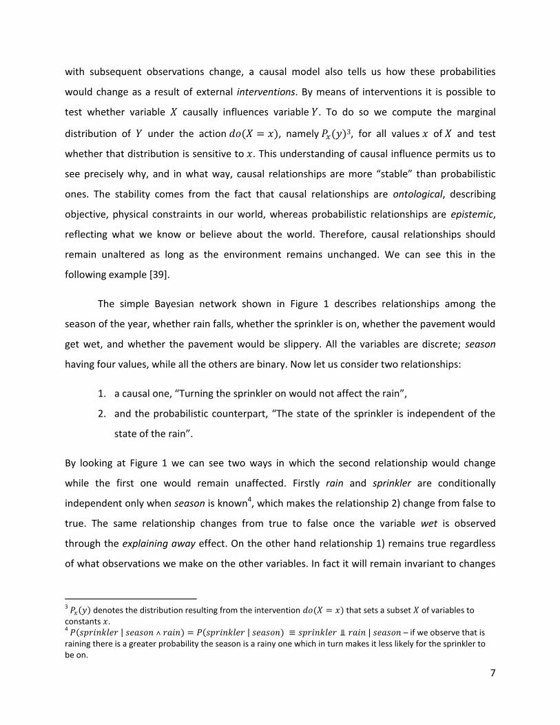
The simple Bayesian network shown in Figure 1 describes relationships among the
season of the year, whether rain falls, whether the sprinkler is on, whether the pavement would
get wet, and whether the pavement would be slippery. All the variables are discrete; season
having four values, while all the others are binary. Now let us consider two relationships:
1. a causal one, “Turning the sprinkler on would not affect the rain”,
2. and the probabilistic counterpart, “The state of the sprinkler is independent of the
state of the rain”.
By looking at Figure 1 we can see two ways in which the second relationship would change
while the first one would remain unaffected. Firstly rain and sprinkler are conditionally
independent only when season is known4, which makes the relationship 2) change from false to
true. The same relationship changes from true to false once the variable wet is observed
through the explaining away effect. On the other hand relationship 1) remains true regardless
of what observations we make on the other variables. In fact it will remain invariant to changes
3 denotes the distribution resulting from the intervention that sets a subset of variables to
constants . 4 – if we observe that is
raining there is a greater probability the season is a rainy one which in turn makes it less likely for the sprinkler to be on.
8
in all mechanisms shown in this causal graph and therefore we can see it exhibits greater
robustness [39].
Figure 1 – A simple causal network
Another consideration we should make is that it is understood that independence
assumption carried by the DAG does not necessarily imply causation. On the other hand the
stability of causal relationships mentioned above is the reason for the ubiquity of DAG models in
AI applications. Therefore, probabilistic relationships may be helpful in hypothesizing initial
causal structures from uncontrolled observations, but once the acquired knowledge is cast in
causal structures the probabilistic interpretation tends to be forgotten.
2.1.3 Causal structure learning
Looking at the world as consisting of a collection of causal systems and each system
consisting of a set of observable causal variables we can translate such systems into causal
Bayesian networks. To learn such a network we observe causal systems on a set of trials on
which each variable takes a specific value [20]. For example an autonomous intelligent system
attempting to build a workable model of its environment cannot rely exclusively on
preprogrammed causal knowledge; rather, it must be able to translate direct observations made
using its sensors to cause-and-effect relationships [39].
The problem lies in the fact that data thus collected comprises a set of passive
observations on which we can perform statistical analysis driven by covariation instead of
causation. Learning causal relationships from raw data has been on philosophers' wish list since
SLIPPERY WET SEASON
RAIN
SPRINKLER
9
the 18th century. The approach taken to achieve this goal has been to try understanding the
process by which humans acquire causal relationships and trying to build a computational
model based on it [39].
Human inference of causal relationships is taken to rely primarily on universal cues such
as spatiotemporal contingency or reliable covariation between effects and their causes as well
as on domain-specific knowledge [33]. Accordingly, most theories of causation invoke an explicit
requirement that a cause precedes its effect in time. Yet temporal information alone cannot
distinguish genuine causation from spurious associations caused by unknown factors – the
barometer falls before it rains yet it does not cause the rain [39]. Humans also heavily reside on
the possibility of repeatedly performing interventions to discover causal laws.
In order to learn the structure of a causal network from raw data we need to make some
assumptions. First, we assume that causal networks can provide reasonable models of the
domain. Sometimes a stronger version of this assumption is required, namely that causal
networks provide a perfect description of the domain. The second assumption states that there
are no latent or hidden variables that affect the observable variables [37]. This assumption does
not hold in all domains and we will see that it does not hold in the domain of molecular biology
when dealing with microarray experiments.
From the above assumptions it follows that one of the possible structures over the
domain variables is the “true” causal network. However, from observations alone it is not
possible to distinguish between causal networks that belong to the same equivalence class. In
consequence four different approaches have been developed: constraint-based learning, score-
based learning, Bayesian model averaging and hybrid approaches.
Constraint-based learning methods view a Bayesian network as a representation of
independencies. They try to test for conditional dependence and independence in the data in
order to find a network, or more precisely an equivalence class of networks, that best explains
them. Constraint-based methods are quite intuitive. They decouple the problem of finding
structure from the notion of independence. They also follow more closely the definition of
Bayesian networks: we have a distribution that satisfies a set of independencies, and our goal is
10
to find the equivalence class for this distribution [55]. Unfortunately, these methods can be
sensitive to failures in individual independence tests. It suffices that one of these tests return a
wrong answer to mislead the network construction procedure [45].
Score-based methods, also known as search-based, view Bayesian networks as specifying
statistical models and address learning as a model selection problem. All of them operate on the
same principle: we define a hypothesis space of potential models — the set of possible network
structures we are willing to consider — and a scoring function that measures how well the
model fits the observed data. Our computational task is then to find the highest-scoring
network structure. The space of Bayesian networks is a combinatorial space, consisting of a
super-exponential number of structures — . Therefore, the problem translates to
optimization problem. There are very special cases where we can find the optimal network. In
general, however, the problem is (as usual) NP-hard, and we resort to heuristic search
techniques. Score-based methods consider the whole structure at once; they are therefore less
sensitive to individual failures and better at making compromises between the extent to which
variables are dependent in the data and the “cost” of adding the edge. The disadvantage of the
score-based approaches is that they pose a search problem that may not have an elegant and
efficient solution [55].
Hybrid approaches combine the two learning methods described above, and are
sometimes called search-and-score-based methods [55].
Finally, instead of attempting to learn a single structure the Bayesian model averaging
methods generate an ensemble of possible structures. These methods extend the Bayesian
reasoning and try to average the prediction of all possible structures. Since the number of
structures is immense, performing this task seems impossible. Yet, for some classes of models
this can be done efficiently, and for others we need to resort to approximations [31].
2.1.4 State of the art algorithms
Here we will take a look at the various algorithms devised for learning causal Bayesian
network structures. Since there are many such algorithms differing only in the details, such as
the measure employed for network scoring, only an overview will be presented.
11
2.1.4.1 Score-based methods
Let us start with the scoring-based algorithms. Their main difference is the metric used
for scoring the network which is employed by all algorithms except when performing an
exhaustive search5. The metrics differ in the assumptions they require, e.g. the type of data
(discrete or continuous). Some of the metrics used are listed below.
Maximum likelihood - measures the strength of the dependencies between variables
and their parents. In other words, it prefers networks where the parents of each variable are
informative about it. The maximum likelihood network will exhibit a conditional independence
only when that independence happens to hold exactly in the empirical distribution. Due to
statistical noise, exact independence almost never occurs, and therefore, in almost all cases, the
maximum likelihood network will be a fully connected one. In other words, the likelihood score
overfits the training data. [6, 31]
Bayesian information criterion (BIC) - the score exhibits a trade-of between fit to data
and model complexity: the stronger the dependence of a variable on its parents, the higher the
score; the more complex the network, the lower the score [6, 43].
Akaike information criterion (AIC) – can be generally used for the identification of an
optimum model in a class of competing models. It is a measure of the lack-of-fit of the chosen
model and the increased unreliability of the chosen model due to the increased number of
model parameters. The best approximating model is the one which achieves the minimum AIC
in the class of the competing models [6, 42].
Bayesian metric with Dirichlet priors and equivalence (BDe) - evolved from the search
for a network with the largest posterior probability, given priors over network structures and
parameters. It is based on the concept of sets of likelihood equivalent network structures,
where all members in a set of equivalent networks are given the same score. Used only with
discrete data [6, 51].
5 Because of the triviality and practical infeasibility for networks with more than a small number of variables it
won't be included in the list.
12
Bayesian metric with Gaussian priors and equivalence (BGe) – BDe counterpart for
continuous data [31].
Mutual information tests (MIT) - measures the degree of interaction between each
variable and its parents. This measure is, however, penalized by a term related to the Pearson
test of independence. This term attempts to re-scale the mutual information values in order
to prevent them from systematically increasing with the number of variables [6].
When we fix the scoring metric we still need to decide the rules that will drive the
searching process. The rules describe changes made to the structure at each step of the
algorithm. They can be made either on a local scale (atomic) such that only one edge gets
added, removed or changes the directionality, or on a larger scale (global) when the structure
can change substantially [37].
The simplest and most commonly used is the greedy algorithm, which at each step looks
for the change in the structure with the best score. This procedure suffers from the fact it has a
high probability of poor performance because of ending up in a local minima/maxima. On the
other hand, more complex solutions, such as using metaheuristics (Hill-Climbing, Genetic
algorithm, Tabu search, Simulated annealing,…) still offer no guarantee of finding the best
solution but are less likely to get stuck with a low fitting structure [24].
2.1.4.2 Constraint-based methods
We continue by considering some of the constraint-based methods. Unlike the score-
based methods which always return a fully oriented Bayesian network or a set of networks,
these methods in general will return only an equivalence class, usually in the form of a single
PDAG. The learning process is for most algorithms performed in two phases. In the first phase
the algorithm looks for (in)dependencies using one of the possible independency tests and
outputs the network skeleton6. The second phase tries to orient as many edges by following a
set of rules [1, 2, 4, 9, 31, 32, 39, 45].
6 The skeleton of a DAG is a graph having the same nodes and edges, but all edges being undirected.
13
The commonly used algorithms are IC (inductive causation)[39, 45], SGS (Spirtes,
Glymour and Scheines) [39, 45], PC (Peter and Clark) [39, 45], Incremental Association Markov
Blanket (IAMB or IA) [49], TPDA (Three Phase Dependency Analysis) [8] and RAI (recursive
autonomy identification) [52]. Their short descriptions are given below.
IC – the algorithm starts with the empty graph7 and for each pair of variables and
searches for a subset of nodes 8 such that they are conditionally independent given . If
no such subset exists it adds an undirected edge between and . Once the undirected graph
has been constructed it orients the edges. First it looks for all nonadjacent pairs of variables
and that have a common neighbor and checks if contains . If that is not the case then
it orients the edges to get the v-structure . It ends by trying to orient as many
undirected edges as possible such that any alternative orientation would yield a new v-structure
or a directed cycle.
SGS – same as the IC algorithm except it starts with a fully connected graph and
proceeds by removing edge by edge.
PC – based on the previous two algorithms. It starts with a fully connected graph and
continues with a systematic search for the sets . First it starts with of cardinality zero,
then cardinality 1, and so on; meanwhile edges are removed from a complete graph as soon as
separation is found. This refinement enjoys polynomial time complexity in graphs of finite
degree, because at every stage the search for a separating set can be limited to nodes that are
adjacent to the two taken into consideration for independence. The simplicity and efficiency of
this algorithm are the reasons for choosing it to be the base algorithm for our solution and
therefore it will be discussed in greater length later on.
IA - consists of two phases, a forward and a backward one. An estimate of the Markov
blanket for a variable , denoted as , is kept in the set . In the forward phase all
variables that belong in and possibly more (false positives) enter while in the
backward phase the false positives are identified and removed so that in the
7 Graph containing all the nodes but no edges between them.
8 A subset of nodes that does not contain and .
14
end. The heuristic used in IA to identify potential Markov blanket members in the first phase is
the following: start with an empty candidate set for the , and admit into it (in the next
iteration) the variable that maximizes a heuristic function . Function should
return a non-zero value for every variable that is a member of the Markov Blanket for the
algorithm to be sound, and typically it is a measure of association between and given .
In backward conditioning, the second phase, we remove one-by-one the features that do not
belong to the by testing whether a feature from is independent of given the
remaining .
TPDA – as the name states the algorithm has three phases: drafting, thickening and
thinning. In the first phase the algorithm computes mutual information for each pair of nodes as
a measure of closeness, and creates a draft based on this information. The draft is a singly
connected graph (a graph without loops). In the second phase, the algorithm adds edges to the
current graph when the pairs of nodes cannot be separated using a group of CI tests. The result
of the second phase contains all the edges of the underlying dependency model given that the
underlying model is monotone DAG-faithful9. In the third phase, each edge is examined using a
group of CI tests and it will be removed if the two nodes of the edge are conditionally
independent. The result of this phase contains exactly the same edges as those in the
underlying model when the model is monotone DAG-faithful. At the end of this phase, the
algorithm also carries out a procedure to orient the edges of the learned graph. This procedure
may not be able to orient all the edges. The complexity of this algorithm is . It has been
shown that the monotone DAG-faithfulness assumption together with the faithfulness
assumption restricts the class of possible Bayesian network structures to ones for which the
optimal solution can be found in
RAI - starting from a complete undirected graph and proceeding from low to high
cardinality of separation sets, the RAI algorithm uncovers the correct pattern of a structure by
performing the following sequence of operations: test of CI between nodes, followed by the
9 The assumption states that the (conditional) mutual information between a pair of variables is a monotonic
function of the set of active paths between those variables. The more active paths between the variables the higher the mutual information.

15
removal of edges related to independences, edge orientation according to rules (same ones as
in the IC algorithm), and graph decomposition into autonomous sub-structures. For each
autonomous sub-structure, the RAI algorithm is applied recursively, while increasing the order
of CI testing. While we have already seen the first two steps in other algorithms we will take a
closer look at the last one. Decomposition into separated, smaller, autonomous sub-structures
reveals the structure hierarchy. Decomposition also decreases the number and length of paths
between nodes that are CI-tested, thereby diminishing, respectively, the number of CI tests and
the sizes of condition sets used in these tests. Both reduce computational complexity.
Moreover, due to decomposition, additional edges can be directed, which reduces the
complexity of CI testing of the subsequent iterations. Following decomposition, the RAI
algorithm identifies ancestor and descendant sub-structures; the former are autonomous, and
the latter are autonomous given nodes of the former.
After looking at the description of the constraint-based algorithms we see that each
resides on testing for conditional independence. In principle, each could use any of the tests
that will be mentioned shortly. The tests differ in the data they can be applied to, either discrete
or continuous, but all of them test only for linear dependencies. It has been argued that
datasets in different domains are known to have a high number of non-linear dependencies
between the variables making the use of this test inappropriate [27]. The most commonly used
tests are: Pearson’s chi-squared test, Fisher’s Z test and mutual information. [45]
Mutual information - measures the information that and share. It measures how
much knowing one of these variables reduces uncertainty about the other. For example,
if and are independent, then knowing does not give any information about and vice
versa, so their mutual information is zero. At the other extreme, if and are identical then all
information conveyed by is shared with . That is, knowing determines the value of and
vice versa. It can be used with both continuous and discrete data. The estimation is sometimes
improved through combination with other information by making it closer to the value of the
provided information, and by doing so we get the shrinkage estimator of mutual information. To
calculate the mutual information we use formulas (4) and (5) for discrete and continuous case
respectively [58].
16
∑∑ (
)
∫ ∫ (
)
Pearson’s chi-squared test ( ) - tests a null hypothesis, the one stating that the
frequency distribution of certain events observed in a sample is consistent with a particular
theoretical distribution. The events considered must be mutually exclusive and have total
probability of one. A common case for this is where each event covers an outcome of a
categorical variable. Therefore, it can be used only for discrete datasets. When testing
independence of variables we use the following formula:
∑∑( )
(∑
) (∑ )
where and are the number of rows and columns respectively, is the total sample size, and
is the observed frequency count at level of the first and at level of the second variable. A
chi-squared static larger than the critical point (0.05) is commonly interpreted by applied
workers as justification for rejecting the null hypothesis, stating the variables are independent
[60].
Fisher’s Z test – is used when dealing with continuous Gaussian random variables. After
performing Fisher's z-transformation of the partial correlation, the test statistic has value
√
where the transformation is defined as

17
(
)
and the recursive form of the partial correlation as
√ √
The terms in the above formulas are: – the sample size; – separation set; – variables
being tested for independence given . In a multivariate normal distribution, zero partial
correlation is equivalent to conditional independence therefore the null hypothesis is
The test statistic is (asymptotically for large enough ) standard normally distributed. We reject
the null hypothesis with confidence if the test statistic is greater than
(
)
where is the cumulative distribution function10 of a Gaussian distribution with zero mean
and unit standard deviation [57, 59].
10
It describes the probability that a real-valued random variable with a given probability distribution will be found at a value less than or equal to . In the case of a continuous distribution, it gives the area under the probability density function from minus infinity to .
18
2.2 Ontology
2.2.1 Introduction
Over the last few years ontologies have emerged as means of providing a formal and
structured representation of knowledge which can range from generic real world knowledge to
strictly domain-specific (e.g., linguistics, semantic web, biology, etc.). They represent not only a
fixed structure but also the basis for deductive reasoning [14]. The purpose of employing an
ontological representation is to capture concepts in a given domain in order to provide a shared
common understanding of this domain, enabling interoperability and knowledge reuse but also
machine-readability and reasoning about information through inference. They are deterministic
in nature, consisting of concepts and facts about a domain and their relationships to each other.
The most common definition of an ontology is that it is a formal, explicit specification of a
shared conceptualization. That is, an ontology is a description (like a formal specification of a
program) of the concepts and relationships that can exist for an agent or a community of
agents. It provides a shared vocabulary, which can be used to model a domain, the type of
objects and/or concepts that exist, and their properties and relations [13, 14, 28, 29, 34].
The questions we are interested about ontologies are: what are ontologies for, and how
can they be used in the domain of learning Bayesian network structures. To answer the first
question is fairly easy – the purpose of ontologies is to enable knowledge sharing and reuse. The
second question does not have a trivial and surely not a single answer. We will see some
devised approaches in the section “Related works”, but for now we’ll just argue that bringing
additional knowledge could undoubtedly be useful to guide the structure learning process. We
saw that causality cannot be inferred from data alone, thus we will seek help from the
additional information about variables and their relationship in the real world, in form of
ontologies.
2.2.2 Causal relationships
Except for “is a”, which is implied by the subclass statements, relationships in ontologies
are user defined and domain specific (e.g. “father of”, “teaches”, “synonymy”, etc.).
Relationships that we are interested in are those that could imply some kind of causal
19
relationship between the ontology terms, which could be in turn directly translated into
directed edges of a causal Bayesian network.
We will take a closer look by introducing a simple example. The ontology presented in
Figure 2 could be part of some larger disease ontology which deals with disease taxonomy, the
relations of diseases and their symptoms, the location of the disease, etc. The larger ontology
could also have other relationships as well as a more intricate taxonomy.
The relationships in this example are: “is_a”, “located_in”, and “has_symptom”. The
“is_a” relationships, also called subclass relationship, is implicit and it follows from the class
subsumption statements formally written as
which we interpret as “Subclass is included in Superclass”, or alternatively and less formally “All
the things from the world that are Subclass are also Superclass”. The relation is reflexive,
antisymmetric and transitive11. From what we have seen earlier, it is clear that this relationship
would not do as a causal one, which we know to have quite different properties than the ones
listed for the “is_a” relation. The simple informal example of “Cause is_a Effect” would suffice
to back up our intuition.
Next we will consider the user-defined “located_in” relationship. We can see that even
though its properties are different from the “is_a” relationship it still does not have a causal
meaning. The relation is irreflexive, asymmetric and transitive.
In the end there is the “has_symptom” relation, which is also user-defined and its
properties differ from both previously mentioned relationships. It is irreflexive, asymmetric and
transitive. These are the properties we want for a causal relationship in order to include it in our
causal Bayesian networks. As we can see the “has_symptom” relation does imply causation. The
disease is the cause for symptoms to arise. Therefore, when the ontology states that a disease
has some symptoms it means that the symptoms are a consequence of (they are caused by) the
11
Fromally defined in the appendix section 7.1.

20
disease. Of course, not all relationships that have these properties are causal relationships. For
example, we can think of an ontology about humans and their customs, which has a relationship
“bigger than”. This relation does not have a causal interpretation because the statement -
Elephant “bigger than” Bunny – does not imply that elephants are the causes of bunnies even
though the relation is irreflexive, asymmetric and transitive.
Figure 2 – An example ontology
In the discussion above we argued that some of the relationships can be regarded as
causal. But in the ontology the relationships are not defined for each two terms for which the
relationship holds but only for their most specific ancestors. This we can see in Figure 2 if we
consider the relationship of the “Hodgkin’s lymphoma” and “Neck lymph node swelling” nodes.
Thing
Disease Symptom
Cancer
Lymphoid
cancer
Hodgkin's
lymphoma
Lymphocytes
Lymph node
swelling
Neck lymph
node swelling
Armpit lymph
node swelling
is_a is_a
is_a is_a
is_a
is_a
is_a is_a
has_symptom
has_symptom
located_in
White
blood
cell
Blood
cell
Cell
is_a
is_a
is_a
21
Their connection is not explicitly stated but it can be easily inferred since the latter is a “Lymph
node swelling” which is in relation “has_symptom” with the “Hodgkin’s lymphoma” node.
Which tells us that the “is_a” and “has_symptom” relationship form chain rules that can be
formalized as
In order to infer if some relationship holds between to terms, either directly or indirectly, we
will have to reason over the ontology by means of an inference engine usually referred to as a
reasoner.
2.2.3 Reasoning
Reasoning is the process of inferring logical consequences from a set of explicitly
asserted facts or axioms. The process is performed by a reasoner which typically provides
automated support for reasoning tasks such as classification and querying. Reasoning is needed,
as we have already seen in the previous example, because knowledge in an ontology might not
be explicit and a reasoner is required to deduce implicit knowledge so that the correct query
results are obtained.
For our needs we will need a reasoner to find out if there exists a causal relationship
between ontology terms. Unfortunately, the available reasoners (FaCT++, HermiT, Pellet, etc.)
do not provide built-in methods for performing such inference. Therefore, it was needed to
think of a procedure that will rely on the available functionalities, mainly subclass and
superclass retrieval.
Before we continue by showing the steps needed to perform the needed inference
process, we will introduce some notation to make it more understandable. We have already
seen subsumption statements which use the operator and now we will introduce another
class expression which deals with relations. It is the qualified existential restriction usually
written as

22
and our procedure will heavily rely on it. It is nothing more than a complex class denoting the
set of all objects of the universe that are in relation “relation” with the objects from “class”. For
example, is the set of all objects that have female children.
Now we can specify the steps of the process for inferring the presence of a causal
relationship between two terms that we will refer to as Cause and Effect.
1. Find the superclasses of Effect.
2. Find all the classes that have a causal relation to the classes retrieved in step 1.
3. Find if the set of the classes retrieved in steps 2 contains Cause.
4. If it does, there exists a causal relationship between Cause and Effect.
The explanation for the given procedure is the following. First in steps 1 and 2 we want
to find all the classes that are causally related to the Effect class or any of its ancestors, since
when a class is related to an ancestor, the relation also influences its descendant classes. If the
Cause class is among the classes that are causally related to the Effect or some of its ancestors
we can infer that there exists a causal relationship between the two.
It might be tempting to consider taking into account subsets of the Effect class or
subsets/supersets of the Cause class, but we will show that such inference is not sound. When
we consider the subsets of the Effect class it is clear that if we have a cause that causally
influences a subset of the descendants this relation does not tell us anything about its relation
to the Effect class. Each descendant has an additional chunk of information which might be the
reason for the presence of the causal relation. Even if all the descendants would be causally
related to the Cause class it would not be enough to justify the existence of the relation for the
Effect class because there might be other subclasses not yet present in the ontology which are
not causally related to the Cause class. The same kind of reasoning can be used when
considering subclasses of the Cause class.
On the other hand if we consider including the superclasses of the Cause class when
looking for its relation to the Effect class, two problems arise. The first one being the possibility
that situations might arise in which a class is causally related to its own ancestor. The intuition
23
behind it is that those relations are to general because they involve quite general terms. For
example, in the Biological processes ontology cases as the following arise: the ancestor of the
Cause term is “regulation of biological process” which is related to “biological process” through
the “regulates” relation, but the Cause term is itself a “biological process” (which is also the top
class12 of the ontology). Such a relation tells us very little since it can be understood as a
tautological statement. A more general rule would be to disregard relationships that are “too
high” in the hierarchy. But it is not possible neither to state how high is too high nor to know
during the reasoning process know where the terms reside since the ontologies are represented
using DAG which does not have a fully defined ordering of terms.
The other problem that would arise if we were to consider Cause class superclasses is
related to the previous one but is more sever. Let us consider four classes , , and , where
and are subclasses of and respectively, moreover and regulate and
respectively. Now, if we were to try inferring a causal relationship between and any sibling of
by looking at both the causal relation of and . If we were to consider superclasses of we
would find a causal relation because of the relation existing between and . But such a
conclusion is wrong because we know for a fact that causally influences only while the
conclusion drawn would be that it is causally related not only ’s ancestors but also to all its
siblings.
The exact way the described process will be used is going to be described in subsequent
sections. Now we will turn to look at some related works in which ontologies were used in the
process of learning the Bayesian network structure.
12
The top class of an ontology is its root node. That is, all the classes in the ontology are in descendants of the top class. See also footnote 17.
24
3 Related work
Here we will discuss some approaches taken to combine the knowledge present in
ontologies and Bayesian networks. They are concerned with mapping the ontology structure to
a Bayesian network or representing uncertain knowledge in ontologies. The main idea behind
these approaches is exploiting the structure similarity between Bayesian networks and
ontologies, namely the underlying DAG.
The first work was done by E. Helsper and L. van der Gaag [22] and it dealt with devising
a knowledge-engineering methodology for constructing and maintaining Bayesian networks.
Their approach makes use of a manually constructed ontology which gets translated into a BN.
The ontology here is used to make it easier for experts to model the domain knowledge that will
be needed in the BN. In this approach as it will also be the case in others, there is no existing
ontology whose knowledge is being exploited but it is just a more human-readable
representation of the knowledge that gets translated into a BN.
Later, an extension of the OWL language for ontologies was proposed by Z. Ding and Y.
Peng [14] in order to incorporate probabilistic knowledge which would allow for simpler
translation process that would in turn allow probabilistic reasoning over the constructed BN.
Again, we have a mapping from the ontology to the BN structure with the additional
information of probabilistic markups attaching probabilities to classes and relations which are
used for constructing conditional probability tables. A later extension of his approach allowed
for automatic ontology mapping between ontologies.
A. Devitt, B. Danev and K. Matusikova [13] continued on the idea from Helsper and van
der Gaag to devise an algorithm for translating ontologies into Bayesian networks in the
telecommunications domain. In this system, the ontology model has the dual function of
knowledge repository and facilitator of automated workflows while the generated BN serves to
monitor effects of management activity, forming part of a feedback loop for self-configuration
decisions and tasks. All in all this work just puts in practice the previous idea and deals with the
implementation issues more thoroughly.
25
In the medical domain Jeon and Ko [29] proposed a semi-automatic algorithm which
extracted nodes from an ontology and let the expert draw the causal relationships between
them. Such an approach only facilitates the BN construction by providing the expert with a user
friendly interface.
For the same domain in a later paper Zheng, Kang and Kim [54] proposed another way
for incorporating uncertainty in ontologies. Their approach had the goal of both adding
uncertainties in an ontology and allowing for the probability distribution to be updated by
adding new data. They did it by adding additional (probabilistic) information into the ontology
and upon the presence of new data the BN gets extracted from the ontology and its CPTs get
updated. This approach uses the benefits of both BNs and ontologies, each bringing its full
functionality into the system.
Ishak, Leray and Amor [28] again deal with the translation of the ontology into the BN
structure with the difference that they use objective oriented Bayesian networks (OOBN). The
advantage of using OOBN is in the fact that nodes can be assigned properties and be
represented in a hierarchy making them more similar to ontologies than regular BNs. It is
straightforward to see that by means of the hierarchy it is possible to translate the ontologies’
“is_a” relationship into the OOBN.
The last and closest approach to the one discussed in this work was proposed by
Messaoud, Leray and Amor [34]. They use the knowledge and functionalities present in both
models to transfer the knowledge both ways. First they use the knowledge present in the
ontology to constrain the possible Bayesian network structures and guide the learning process.
In a latter phase the BN structure is used to update the ontology structure by adding newly
found causal relationships between terms. Unlike our approach they impose the following
constraints:
- each causal graph node must be modeled by a corresponding concept in the domain
ontology,
- and the causal relations have to be defined between all elements of the ontology for
which it holds.

26
These constraints do not allow the usage of existing ontologies but only of those
designed by experts, while in our work we would like to take advantage of preexisting
ontologies. These ontologies are usually curated by experts and constantly evolving.
In the next section we are going to look at our solution which was inspired by
ideas discussed in the aforementioned works.

27
4 The algorithm
The main goal of the proposed approach is learning the Bayesian network structure
using a constraint-based algorithm and exploiting the knowledge present in the ontology to try
orienting the remaining undirected edges. By using only the former will in most cases result in
forming a PDAG structure. For this purpose we can use one of many algorithms mentioned in
earlier sections. Which one depends on the characteristics of the data we are dealing with and
most of all on the quality of results produced. In our case it will be a variant of the PC algorithm
which uses continuous data. The knowledge present in the ontology can be used to infer
connections between variables and it can be placed at different stages:
- before using the constraint-based algorithm in order to find connections in order to
lower the number of possible structures,
- after using the constraint-based algorithm but before it assigns edge orientations13,
- after the constraint-based algorithm has produced a PDAG structure to infer the
orientation of undirected edges,
- and same as in the last case with the additional task of checking the correctness of
the orientation of the directed edges.
Moreover, the ontology could be used in combination even with a score-based approach but we
are not going to deal with it in this work.
Our approach tried to lesser the constraints imposed upon the format of the ontology in
order to allow using popular existing ontologies from different fields such as biology, medicine,
chemistry, and others. All the user has to define is the causal relationship that is present in the
ontology such as “has_symptom” or “regulates” since each ontology contains different such
relations.
One important question is how do we connect the BN variables to the concepts present
in the ontology? The approaches we have seen in the previous section make either the user
select the concepts to be used or just use all the leaf concepts. In our approach we take a
13
Given the algorithm performs the processes of finding edges and orienting them in different stages.
28
somewhat different approach where we annotate the nodes of the BN with terms from the
ontology. This was done by taking into consideration how genes in the bioinformatics field get
annotated with ontology terms. Each gene can have different functions and be part of different
pathways. Therefore, a single annotation is not enough. In the same way we annotate our
variables in the BN with terms of the given ontology. This way we are not bound to having an
ontology with all the variables present in the BN and we can also transfer more information to
the BN. On the other hand we need to provide a mapping between the BN variables and the
ontology terms. Such mappings already exist in some domains, for example in bioinformatics
between genes and terms from the Gene Ontology.
4.1 Steps of the algorithm
We have seen all the needed components for our algorithm and now we can specify its
steps and afterwards go through them in detail. As we mentioned earlier the ontology can be
used at different points of the algorithm but in this work only one will be considered leaving the
other options for future work. The algorithm will go through the following steps:
1. Data preparation
2. Structure learning with PC algorithm
a. Independence testing
b. Edge orientation
3. Node annotation
4. Inferring undirected edge orientation from the ontology
4.1.1 Data preparation
This step is strictly speaking not part of the algorithm but is crucial and the result highly
depends on it. For the purposes of our algorithm it won’t be needed to discretize the data
however it is required to be in a proper format and missing values have to be taken care of. The
downside of this approach is not having the possibility to deal with categorical variables for
which a different version of the PC algorithm or a different algorithm altogether should be used.
Since the formatting part of the data preparation step involved only parsing of the
dataset we are not going look into it. However, dealing with missing values requires some

29
attention. Datasets containing experimental data usually contain a fair amount of missing values
especially in high-throughput methods such as microarray experiments. To sanitize such a
dataset a couple of methods have been devised which try to impute the missing value with a
value similar to values of that the variable in other experiments. One such method which was
used in our work is the kNNimpute algorithm [48].
The kNNimpute algorithm works as follows. If a variable misses the value for the first
experiment, the algorithm will go looking for other variables that have similar values in other
experiments. In the end it will assign the value that is calculated as a weighted average of the
nearest variable values in the first experiment. The algorithm can be used with different metrics
for calculating the distance. In our case the distance metric used was the Euclidian one. It has
been shown empirically that using this metric gives the best results [48].
The only parameter that influences the output of the kNNimpute algorithm is the
minimum percentage of data values present for a variable over the experiments. This threshold
was set to a quite low value (10%) in order to retain as many variables as possible. By doing so
we have lessened the importance of having a dataset that faithfully resembles the real data, and
are more concerned with having as much data as possible.
4.1.2 Structure learning with PC algorithm
We have already given some overview of this algorithm in an earlier section. Now we will
give a closer look at the details regarding its implementation and the specific variant used in our
algorithm. We will start by looking at the steps of the algorithm and later specify the conditional
independency test employed.
The steps of the PC algorithm are described in Figure 3 where we can see that some
steps offer a high degree of flexibility allowing different approaches. For example, in step 2) any
conditional independency test would do, but also different orders of variable selection can be
used. In our work we used the Fisher’s Z test and the simplest ordering, checking sequentially
pairs of variables in the order variables appear in the dataset.
30
The Fisher’s Z test was explained in detail in section 2.1.4.2. We used it with the
parameter 14 having value 0.05, meaning that the probability of incorrectly rejecting the null
hypothesis is 5%. This is the most commonly used value and it will serve our purposes.
Steps 1) and 2) produce an undirected graph while steps 3) and 4) try to orient as many
edges as possible. The inference of edge orientation through the knowledge present in the
ontology could be done before step 1), after step 2), or as it will be in our case after the
algorithm finishes.
Step 4) is also given in a descriptive way which allows us to take different approaches. It
has been shown the four rules listed in Figure 4 are required for obtaining a maximally oriented
PDAG. Moreover, they are sufficient, meaning that repeated application will eventually orient
all edges which are common to the graph’s equivalence class [39].
This algorithm works under the assumption of absence of latent structures15. They
require a special treatment, because the constraints a latent structure imposes upon the
distribution cannot be completely characterized by any set of conditional independence
statements.
4.1.3 Node annotation
In order to use the PDAG produced from the previous step together with the ontology
we need to make a connection between ontology concepts and the BN variables. As we have
discussed earlier, this is done by assigning a set of ontology terms to each variable. We assume
that there exists a mapping created by experts which faithfully resembles the state of the world
for the domain of interest.
14
Usually refered to as significance level. 15
A latent structure is one having only a subset of variables observed. By making the above assumption we assume that the variables from the dataset are indeed all the variables present in the system being modeled. This is a strong assumption which is rarely true.

31
1. Orient into whenever there is an arrow such that and are
nonadjecent.
2. Orient into whenever there is a chain .
3. Orient into whenever there are two chains and
such that and are nonadjecent.
4. Orient into whenever there are two chains and
such that and are nonadjecent and and are adjecent.
Figure 3 - PC algorithm
1) Form the complete undirected graph on the vertex set .
2) .
Repeat
Repeat
Select an ordered pair of variables and that are adjacent in such
that has cardinality greater than or equal to ,
and a subset of of cardinality , and if and
are d-separated given delete edge from and record in
and ;
Until all ordered pairs of adjacent variables and such that
has cardinality greater than or equal to and all subsets
of of cardinality have been tested for d-separation;
;
Until for each ordered pair of adjacent vertices , , is of
cardinality less than .
3) For each triple of vertices , , such that the pair , and the pair , are each
adjacent in C but the pair , are not adjacent in , orient as
if and only if is not in .
4) In the partially directed graph that results, orient as many of the undirected edges as
possible subject to two conditions: any alternative orientation would yield a new v-
structure; or any alternative orientation would yield a direct cycle.
– set of nodes adjacent to in graph
– set of node d–separating nodes and
Figure 4 – PC algorithm rules
32
4.1.4 Inferring undirected edge orientation from the ontology
We discussed the idea behind this step in the section where we dealt with the reasoning
process. There we considered only how to infer if there exists a causal relationship between two
terms. But in our approach each variable is annotated with a set of terms. Therefore, to infer a
causal relationship between two variables we will have to look for a presence of a causal
relationship between every pair of terms the two variables are annotated with.
For example, for two variables and , such that is annotated with the set of terms
and with the set of terms we will need to check for a causal relation
between terms . By doing
this we will check only if . Therefore, we will also need to check the inverse relation.
For performing the reasoning process we used the HermiT reasoner. Two other
reasoners were tried, Pellet and TrOWL, but they did not perform as well as HermiT [12]. There
are also other reasoners available but they either did not provide an API for Java16 or were not
publicly available.
When considering the DAG property of BNs we could conclude that after finding a causal
relation between two terms we do not have to check the existence in the other direction.
However, in an ontology it is not mandatory for relationships to be acyclic. The simplest
examples are relations such as “friend of” and “sister of” which will be present both ways and
thus form a cycle. But this is also the case for causal relationships such as “regulates”, present in
the GO. Some genes are parts of regulatory mechanisms which involve loops.
One such mechanism is one where we have a gene that starts getting expressed because
of the presence of some chemical in the cell body. This gene gets translated into a protein which
also has the ability to promote the expression of a second gene. Once the concentration of the
protein reaches the threshold value the second gene starts getting expressed. The protein
encoded by the second gene on the other hand acts as a repressor for the expression of the first
gene and therefore we have a regulation loop.
16
Which was used for implementing the algorithm.
33
There is the possibility even of self-regulating loops, when a gene is involved in
regulating its own activity. Even though such loops could be found in an ontology, this case
won’t be considered in our approach.
This kind of cyclic relations cannot be encoded in BNs because it lacks the ability of
representing temporal/dynamic aspects of the system. To do so an extension of the BN model
should be introduced. Even if were to allow this violation it would not be too concerning since
we are only interested in learning the structure and not using the BN for probabilistic inference.
There is another question that needs to be raised, the one asking which edges should
the algorithm try to orient. The simplest approach would be to assume that the constraint-
based structure learning algorithm has found all the independencies and we are left to try
orienting only the undirected edges. On the other hand, from the previous discussion we see
that some orientations might not have been considered because they violate the acyclicity
property. Therefore, it would be worthwhile to consider all edges at the same time validating
the results of the PC algorithm. The problem with this approach is the complexity of task that
will be considered in the following section. This is also the reason for not using this step before
the PC algorithm.
In order to deal with the mentioned complexity the implementation of this step was
done by parallelizing the process such that each thread deals with one edge. The speedup of
this step is therefore proportional to the number of threads/processing units. The
implementation code for this step is given in the appendix section 7.2.
4.2 Complexity analysis
Now that we have seen the steps of the algorithm in detail we are going to consider
their computational cost. The complexity, both space and time, proved to be quite a challenge
when dealing with real-world data. For example the number of genes that get represented as
nodes in the BN from a microarray experiment is in order of thousands. In that case just fully
connecting a graph proves to be a challenge space-wise. In this section we will also show some
optimization steps taken in order to deal with such challenges.

34
However, in this work we will be considering just the complexity of the steps in our
algorithm and not the complexity of tools used, such as the reasoner. Specifically for reasoners,
their performance is usually compared empirically. Tests show that different reasoners perform
differently for different ontologies [12]. In our case we have chosen the reasoner that was the
easiest to integrate and the one best performing on the example we used.
4.2.1 PC algorithm complexity
We will start by considering the complexity of the PC algorithm. More precisely we are
going to put an upper bound on it. If we take that the graph has nodes and let be the
maximal degree of any node. In the worst case, in each iteration, no edge will get removed.
Therefore in the -th iteration we will have to check separation sets of cardinality and for each
of the pairs of variables there are (
) candidate separation sets, which gives us
a total of
∑(
)
independency tests. Such worst case examples are highly unlikely to be found in any dataset
and the average expected number of independency tests is much lower. Still, the complexity is
polynomial, namely .
For each independency test we use the Fisher’s Z test calculated by the recursive
formula
√
√
Where is the separation set being considered in the -th step and therefore having cardinality
. To calculate this value we need to recursively call three calculations of the coefficient
with separation set having cardinality . Thus we have

35
and therefore
Here stands for number of data values for each variable (number of experiments) and
denotes the number of arithmetic operations needed for each independency test between two
variables with a separation set of cardinality .
As we can see the complexity when considering the number of arithmetic operations
turns out to be exponential. On the other hand by looking at the recursive formula we see that
the complexity can be dealt with if we introduce caching of results since there will be lots of
calls to previously calculated values. For caching results a tree-like structure was implemented
where each path represents a string of node ids and the value at each tree node the value of the
calculated coefficient. The first and second node in the path are the and variables being
tested for independence and the rest of the tree nodes in the path stand for the nodes in the
separation set.
This approach considerably reduces time complexity but also takes into consideration
the space complexity because it is not feasible to cache all the possible results in memory. The
algorithm designed this way has been able to deal with datasets with as many as 6000 variables
in a reasonable amount of time (under 2 min). For comparison most of the publicly available
constraint-based structure learning algorithms struggle with the subset of the same dataset
having around 100 variables.
4.2.2 Ontology inference complexity
The complexity of annotating nodes with ontology terms is linear, straightforward to
deduce and it will not be considered. On the other hand the complexity for the inference by
36
means of the ontology was already hinted. Here we will just formalize it. Let be the maximum
number of ontology terms mapped to any variable. Then for undirected edges we have to
make at most
calls to the reasoner. The first factor stands for checking both orientations, the third factor tells
the number of pairs of terms to be sought for a causal relationship, and the last factor is just the
number of calls to the reasoner for retrieving superclasses and related terms.
Even though the number of calls to the reasoner is quite low, the reasoning process itself
is quite time consuming, especially if the ontology being employed is big. Even though the
performance drastically increases when the inference process gets parallelized, such that each
edge is given its own thread, it still takes a lot of time to perform this step (several hours).
37
5 Example
Now that we have discussed the algorithm we can look at how it behaves on a real-life
example. We have chosen the field of molecular biology because of the amount of standardized
data publicly available, the number of high quality ontologies devised, and of course the
importance of the field. The data we are going to use was produced by a microarray experiment
concerning the yeast cell cycle. The motivation for using this dataset was the fact it has been
used in a number of papers that tried to learn the interaction network of its genes [7, 11, 16, 18,
37, 44]. There are various approaches varying in methods used, while only a small involved
causal Bayesian networks, even though they gave promising results [16, 37].
We will see a brief overview of the data, the ontology employed, and in the end the
results produced by the algorithm. All the resources used are publicly available [61, 62, 63].
5.1 Resources
5.1.1 Yeast cell cycle dataset
This dataset was created as a comprehensive catalog of yeast genes whose transcript
levels vary periodically within the cell cycle. The experiments were done under different
conditions and monitored during equally spaced intervals17. In our work the temporal aspect of
the experiments was not considered, as it was done in other related works, instead it was
assumed that the values are independently drawn from an unknown distribution [16, 37].
The dataset came in an already preprocessed form. It underwent through some standard
transformation processes and it was normalized. To correct for the missing values the
kNNimpute algorithm was used as explained in a previous section. It contains 76 gene
expression measurements of the mRNA levels of 6177 S. cerevisiae open reading frames. Only
small number of them have been proven to be cell cycle regulated (~800) [44].
Most related works use even smaller subsets of the original dataset to test their
algorithms. The only one that considered at least the 800 genes found to be cell cycle regulated
was proposed by Friedman, Linial, Nachman, Pe’er but we were unable to get the results in a
17
Different for each experiment.
38
machine readable format, only as an on-line interactive graph which would require a great
amount of time in order to compare with our results [16].
These smaller datasets are those for which it was found to regulate the production of a
certain important gene, regulating the cell cycle or which are known to be highly over or under
expressed during a specific phase of the cell cycle [44].
5.1.2 Gene Ontology
We decided to use the Gene Ontology since it is one of the most actively used and
maintained ontologies and thus providing high quality knowledge. It is part of a major
bioinformatics initiative with the aim of standardizing the representation of gene and gene
product attributes across species and databases. The project provides a controlled vocabulary of
terms for describing gene product characteristics and gene product annotation data. It has
developed three ontologies that describe gene products in terms of their associated biological
processes, cellular components and molecular functions in a species-independent manner [61].
They cover three different domains:
- cellular component, the parts of a cell or its extracellular environment,
- molecular function, the elemental activities of a gene product at the molecular level,
such as binding or catalysis, and
- biological process, operations or sets of molecular events with a defined beginning
and end, pertinent to the functioning of integrated living units: cells, tissues, organs,
and organisms.
In our example we used the biological processes ontology, being the one containing the
“regulates” relation which can be easily attributed a causal interpretation. A biological process is
series of events accomplished by one or more ordered sets of molecular functions. Examples of
broad biological process terms are cellular physiological process or signal transduction. It can be
difficult to distinguish between a biological process and a molecular function, but the general
rule is that a process must have more than one distinct steps [61].
39
Other than the “regulates” relationship the biological processes ontology also contains
two sub-relationships, namely “positively regulates” and “negatively regulates”. For our
purposes we do not need to distinguish them since we are not interested in the functional form
of the causal relationship but only in the structure of the causal network. On the other hand
some more advanced approaches in the future whose goal goes beyond structure learning could
use this additional knowledge.
The upside of the Gene Ontology from an epistemic point of view, of being organism-
independent is also a downside from a practical point. When dealing with a single organism
(which is usually the case) we have a much bigger ontology of what is actually needed which
considerably affects the performance. Some organism-specific ontologies have been created but
are much too simple and stripped from most of the useful relations present in the complete
one.
In any case we can be sure that the evolution of the Gene Ontology hasn’t stopped,
which is currently being updated on a daily basis, and that it might provide a great deal more of
useful knowledge in the future. Moreover, there are many more ontologies being created that
could be used for supporting causal network structure learning in other domains.
5.1.3 Annotations
For standardization purposes the GO consortium devised also an annotation format,
namely the GAF, currently version 2.0. The format specifies information that needs to be
provided for each annotation of a gene, e.g. the GO id, evidence code and name [61].
A GO annotation consists of a GO term associated with a specific reference that
describes the work or analysis upon which the association between a specific GO term and gene
product is based. Each annotation must also include an evidence code to indicate how the
annotation to a particular term is supported. Although evidence codes do reflect the type of
work or analysis described in the cited reference which supports the GO term to gene product
association, they are not necessarily a classification of types of experiments/analyses. Note that
these evidence codes are intended for use in conjunction with GO terms, and should not be
considered in isolation from the terms. If a reference describes multiple methods that each
40
provides evidence to make a GO annotation to a particular term, then multiple annotations with
identical GO identifiers and reference identifiers but different evidence codes may be made
[61].
The evidence or quality code describes the work or analysis upon which the association
between a specific GO term and gene product is based e.g. manual, automatic or computer
analysis. It has a number of possible values depending on the analysis type. Not all the codes
have the same strength and there exists a hierarchy between them18. They range from manually
curated annotations inferred by direct assays to automatically assigned annotations based on
similarity searches. The former being a highly trusted one, while the latter the least dependable
[61].
The annotations process, in our case, was implemented quite straightforward since we
used a publicly available web service which for a given gene id returns its GO terms. The web
service we used is provided by YeastMine [63] which is specialized for the Yeast (Saccharomyces
cerevisiae) genome. During the annotation process we haven’t considered the evidence code
information, for lack of expertise in the bioinformatics domain and again for testing our
approach on as much data as possible. This may turn out to be a shortcoming and a potential
cause for inferring non-causal relationships. Yet, a simple extension would allow an expert to
use the algorithm only with the evidence codes she finds fit.
The mapping can be also loaded from and saved to a file. In our case it we use a standard
format specified by the GO Consortium, the GAF 2.0 annotation file format.
5.2 Results
Here we will look at the resulting graphs produced by our algorithm. They have been
produced on different subsets of the yeast cell cycle dataset and compared to other
approaches. It wasn’t possible to compare the graph resulting from the complete dataset since
no other algorithm was able to deal with such an amount of data. Before we continue, we will
pose some questions that will guide our review. The questions are the following:
18
It can be seen in the appendix.

41
- Is it possible to find the orientation of undirected edges by reasoning over an
ontology?
- Are the orientations sound?
- How do the results compare to other approaches?
- Is the process feasible on a larger scale?
5.2.1 Algorithm performance
In our first experiment we used a dataset made up from the 800 genes found to be cell
cycle regulated. All the 76 data values for different experiments have been used and treated as
independent observations. The PC algorithm ran for around 4 seconds and produced a graph
with 132 undirected edges and 1251 directed ones. The annotation step assigned a total of 3072
terms to the 800 variables making an average of 3.84 terms per variable. The annotation was
done by using a mapping file, after which the undirected edges were checked for causal
relations between the incident variables. As a result 4 undirected edges have been oriented,
one of which have been found to be bidirectional. Since we know the data to be temporal in its
essence we cannot resolve these ambiguities. The step took around 2 hours and 27 minutes to
complete while being executed in parallel on 3 threads.
From this information we can answer the first and last question. Yes, it is possible to
infer the orientation of some undirected edges and in a similar manner it would be possible to
validate the orientations found in the previous steps. But it is clear that the computational
power needed for performing such an inference, which has resulted in the orientation of only a
small fraction of undirected edges, is more than we would expect to spend for such a
procedure. Especially when knowing that much quicker results could be produced by some
other methods even when sacrificing correctness. As always it is a matter of our needs and the
trade-off we are willing to make.
5.2.1.1 Soundness
To see whether the orientations inferred using the ontology are sound we will inspect
the ontology to see if the semantics of the gene annotations match causal relations. We will
look at two cases:
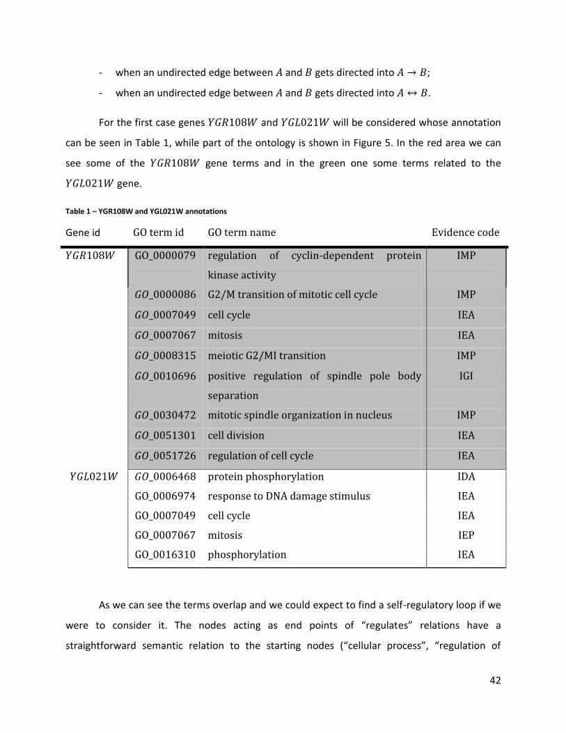
42
- when an undirected edge between and gets directed into ;
- when an undirected edge between and gets directed into .
For the first case genes and will be considered whose annotation
can be seen in Table 1, while part of the ontology is shown in Figure 5. In the red area we can
see some of the gene terms and in the green one some terms related to the
gene.
Table 1 – YGR108W and YGL021W annotations
Gene id GO term id GO term name Evidence code
regulation of cyclin-dependent protein
kinase activity
IMP
G2/M transition of mitotic cell cycle IMP
cell cycle IEA
mitosis IEA
meiotic G2/MI transition IMP
positive regulation of spindle pole body
separation
IGI
mitotic spindle organization in nucleus IMP
cell division IEA
regulation of cell cycle IEA
protein phosphorylation IDA
response to DNA damage stimulus IEA
cell cycle IEA
mitosis IEP
phosphorylation IEA
As we can see the terms overlap and we could expect to find a self-regulatory loop if we
were to consider it. The nodes acting as end points of “regulates” relations have a
straightforward semantic relation to the starting nodes (“cellular process”, “regulation of
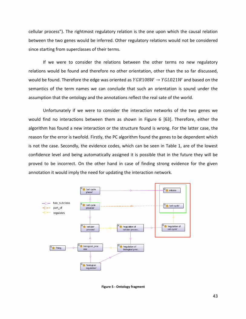
43
cellular process”). The rightmost regulatory relation is the one upon which the causal relation
between the two genes would be inferred. Other regulatory relations would not be considered
since starting from superclasses of their terms.
If we were to consider the relations between the other terms no new regulatory
relations would be found and therefore no other orientation, other than the so far discussed,
would be found. Therefore the edge was oriented as and based on the
semantics of the term names we can conclude that such an orientation is sound under the
assumption that the ontology and the annotations reflect the real sate of the world.
Unfortunately if we were to consider the interaction networks of the two genes we
would find no interactions between them as shown in Figure 6 [63]. Therefore, either the
algorithm has found a new interaction or the structure found is wrong. For the latter case, the
reason for the error is twofold. Firstly, the PC algorithm found the genes to be dependent which
is not the case. Secondly, the evidence codes, which can be seen in Table 1, are of the lowest
confidence level and being automatically assigned it is possible that in the future they will be
proved to be incorrect. On the other hand in case of finding strong evidence for the given
annotation it would imply the need for updating the interaction network.
Figure 5 - Ontology fragment
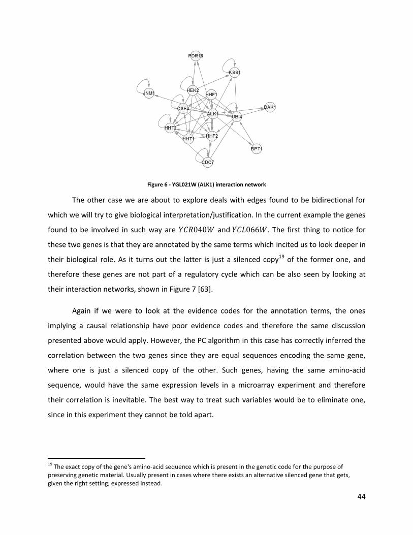
44
Figure 6 - YGL021W (ALK1) interaction network
The other case we are about to explore deals with edges found to be bidirectional for
which we will try to give biological interpretation/justification. In the current example the genes
found to be involved in such way are and . The first thing to notice for
these two genes is that they are annotated by the same terms which incited us to look deeper in
their biological role. As it turns out the latter is just a silenced copy19 of the former one, and
therefore these genes are not part of a regulatory cycle which can be also seen by looking at
their interaction networks, shown in Figure 7 [63].
Again if we were to look at the evidence codes for the annotation terms, the ones
implying a causal relationship have poor evidence codes and therefore the same discussion
presented above would apply. However, the PC algorithm in this case has correctly inferred the
correlation between the two genes since they are equal sequences encoding the same gene,
where one is just a silenced copy of the other. Such genes, having the same amino-acid
sequence, would have the same expression levels in a microarray experiment and therefore
their correlation is inevitable. The best way to treat such variables would be to eliminate one,
since in this experiment they cannot be told apart.
19
The exact copy of the gene's amino-acid sequence which is present in the genetic code for the purpose of preserving genetic material. Usually present in cases where there exists an alternative silenced gene that gets, given the right setting, expressed instead.

45
If we were to look at the two genes as being the same node it would turn out to be a
self-regulatory node which would not be considered by our algorithm.
Figure 7 - YCR040W (MATALPHA1) and YCL066W (HMLAPHA1) interaction networks
The considerations made so far show the importance of the knowledge used for
inferring the network structure. Since we rely on assumption that it reflects the true state of the
world, the produced network is sound under the given assumption. This we saw to be reflected
in the semantics of the ontology terms. The difference between this and other manual
approaches is that our algorithm relies on publicly available and constantly changing data used
also for other purposes. This does not require a domain expert being present every time a
network needs to be constructed but only experts curating publicly available knowledge, which
in this case comes in the form of an ontology and the annotation mappings.
5.2.2 Comparison to other approaches
Now we are left with answering the last question left unanswered which requires
comparing our algorithm to other approaches. Even though the motivation for using the
proposed dataset was because it was referenced by a number of papers dealing with Bayesian
network structure learning, none provide a machine readable BN with all the 800 cell cycle
regulated genes. Most of them deal with only small subset of nodes. For the comparison we
decided to use some of the algorithms made publicly available and compare their resulting
graphs with ours on a randomly chosen subset of the Spellman dataset containing 50 genes.

46
Some of the algorithms might perform poorly because needing data discretization and
we cannot guarantee that the discretization parameters used are the optimal for the given
dataset and algorithm. Another factor that should be taken into account is that some
algorithms, especially the score-based ones, are nondeterministic in nature and might not give
the same answer each time. In our case, the relatively small number of variables taken into
account has proven to produce the same structure on different runs which made it easier to
analyze the results.
Two main characteristics of the resulting graphs will be in our focus: the degree of
similarity of the resulting graphs’ skeletons and the degree of similarity of edge orientations.
This will be done by counting the number of edges the graphs agree and disagree upon, for both
characteristics.
The comparison will be performed with both score-based and constraint-based
approaches which are listed below. A difference between these algorithms is one that we have
already seen earlier but it is worth repeating, namely that constraint-based algorithms in
general produce partially oriented graphs, while score-based always produce totally oriented
graphs.
- Constraint-based: Grow-Shrink, Incremental Association (IA), PC with discrete data
- Score-based: Hill-Climbing (HC) with continuous data, Hill-Climbing with discrete
data, Tabu search
All of the above algorithms were run on the same computer and took a couple of seconds to
finish, except for our approach which took under a second for the step involving the PC
algorithm and a couple of minutes for the ontology inference step.
The results are shown in tables 2, 3 and 4. Table 2 shows number of edges found by the
algorithms, from which we can read out that score-based algorithms prefer highly connected
structures. Such structures are not expected when considering causal networks, for which we
expect that each effect has only a small number of direct causes. On the other hand, constraint-
based algorithms seem to form reasonable structures except maybe for the PC algorithm with
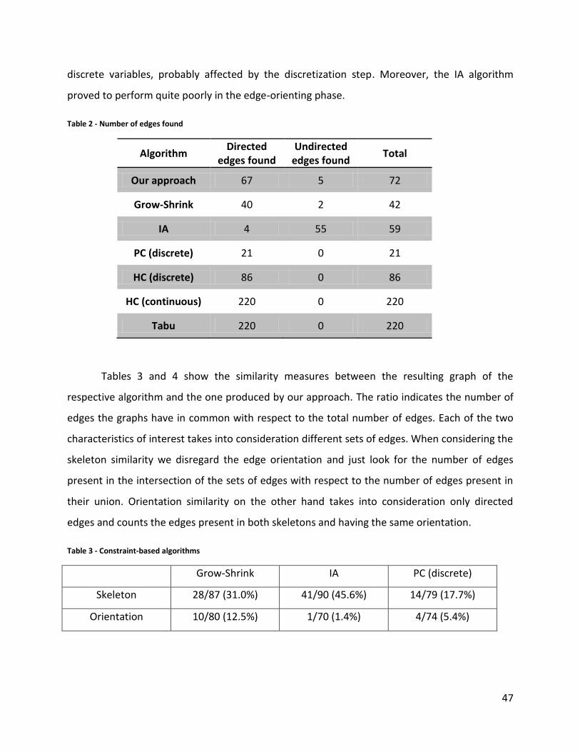
47
discrete variables, probably affected by the discretization step. Moreover, the IA algorithm
proved to perform quite poorly in the edge-orienting phase.
Table 2 - Number of edges found
Algorithm Directed
edges found Undirected
edges found Total
Our approach 67 5 72
Grow-Shrink 40 2 42
IA 4 55 59
PC (discrete) 21 0 21
HC (discrete) 86 0 86
HC (continuous) 220 0 220
Tabu 220 0 220
Tables 3 and 4 show the similarity measures between the resulting graph of the
respective algorithm and the one produced by our approach. The ratio indicates the number of
edges the graphs have in common with respect to the total number of edges. Each of the two
characteristics of interest takes into consideration different sets of edges. When considering the
skeleton similarity we disregard the edge orientation and just look for the number of edges
present in the intersection of the sets of edges with respect to the number of edges present in
their union. Orientation similarity on the other hand takes into consideration only directed
edges and counts the edges present in both skeletons and having the same orientation.
Table 3 - Constraint-based algorithms
Grow-Shrink IA PC (discrete)
Skeleton 28/87 (31.0%) 41/90 (45.6%) 14/79 (17.7%)
Orientation 10/80 (12.5%) 1/70 (1.4%) 4/74 (5.4%)
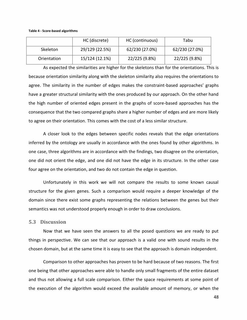
48
Table 4 - Score-based algorithms
HC (discrete) HC (continuous) Tabu
Skeleton 29/129 (22.5%) 62/230 (27.0%) 62/230 (27.0%)
Orientation 15/124 (12.1%) 22/225 (9.8%) 22/225 (9.8%)
As expected the similarities are higher for the skeletons than for the orientations. This is
because orientation similarity along with the skeleton similarity also requires the orientations to
agree. The similarity in the number of edges makes the constraint-based approaches’ graphs
have a greater structural similarity with the ones produced by our approach. On the other hand
the high number of oriented edges present in the graphs of score-based approaches has the
consequence that the two compared graphs share a higher number of edges and are more likely
to agree on their orientation. This comes with the cost of a less similar structure.
A closer look to the edges between specific nodes reveals that the edge orientations
inferred by the ontology are usually in accordance with the ones found by other algorithms. In
one case, three algorithms are in accordance with the findings, two disagree on the orientation,
one did not orient the edge, and one did not have the edge in its structure. In the other case
four agree on the orientation, and two do not contain the edge in question.
Unfortunately in this work we will not compare the results to some known causal
structure for the given genes. Such a comparison would require a deeper knowledge of the
domain since there exist some graphs representing the relations between the genes but their
semantics was not understood properly enough in order to draw conclusions.
5.3 Discussion
Now that we have seen the answers to all the posed questions we are ready to put
things in perspective. We can see that our approach is a valid one with sound results in the
chosen domain, but at the same time it is easy to see that the approach is domain independent.
Comparison to other approaches has proven to be hard because of two reasons. The first
one being that other approaches were able to handle only small fragments of the entire dataset
and thus not allowing a full scale comparison. Either the space requirements at some point of
the execution of the algorithm would exceed the available amount of memory, or when the
49
data was scaled to overcome the memory problem the execution had to be interrupted because
exceeding the amount of time set as the threshold (several hours, whereas our approach would
end in matter of seconds).
The second reason has to do with the degree of similarity of the resulting graphs, which
has proven to be quite low. Each algorithm resulted in completely different network structure,
i.e. different set of independence statements. With such a difference in the results it is hard to
justify any of them. It is reasonable to ask, why do we get such different results? Especially
when trying to infer causal relations which are of particular interest exactly because of their
stability. The best answer we can give as of now is that we lack data, and that the 76 data points
at our disposal are not enough for inferring stable causal relations. On the other hand the lack
of data, which is usually expensive to gather, is the trademark of real world settings and our
main goal is trying to devise an approach that could exploit the small amount of data at our
disposal to infer the underlying causal relations.
This is where our approach differs from others, it exploits publicly available knowledge
of the domain, which is also known to incorporate causal knowledge about its terms. The
downside is that inferring the needed relations from such knowledge is not easy and for now it
is a quite slow process. On the other hand the main advantage is that if the knowledge source,
in our case an ontology, is assumed to reflect the true state the real world, we can regard the
knowledge transferred to our network as stable, which gives us the needed property for giving
the resulting network a causal interpretation.
Another consideration which was mentioned earlier but that maybe has not been
stressed enough is the fact that even though we used a specific constraint-based algorithm,
namely the PC algorithm, as a base for our approach it could be replaced by any other
algorithm. The PC algorithm is in itself quite a simple approach and in the meanwhile more
advanced algorithms have been devised which could, coupled with the ontology-driven phase,
give better results.
The possible extensions of our approach and other considerations will be left for the
next section.
50
6 Conclusion
We have showed in detail the idea behind our approach, how it performs on a real-world
dataset and how it compares to other approaches. Throughout this work we stated the
assumptions needed for the approach to work and in the discussion given in the previous
chapter we covered the pros and cons inherent in our approach.
To conclude, we can state that our idea does provide a valid approach for the problem of
causal Bayesian network structure learning. Even though it did not excel on the example
considered in this work it is likely that it would perform better on some other dataset or given a
better mapping between the ontology terms and the variables. Besides that, the knowledge
transferred from the ontology can be regarded as reflecting the true state of the world, which
provides the needed guarantee for interpreting the resulting Bayesian network as causal one.
On the other hand, some open issues remain. The time required for inferring relations in
the ontology is too high compared to what we would like to see when considering practical
applications. Also, the mapping of the ontology terms to variables might have to be performed
manually for most of the domains which would make the algorithm outside of the molecular
biology domain semi-automatic. Another issue worth considering is whether it is possible to
decide which relations defined in the ontology have causal semantics and in which way do they
relate to other relations, e.g. do they form property chains.
Future works based on this approach can go different ways. One direction is the
optimization of the step for inferring the edge orientation. Other approaches could consider
placing the mentioned step at some other point of the structure learning process or using it for
checking and updating the structure found by the base algorithm. Yet another direction could
consider an in-depth analysis of the base structure learning algorithm focused on finding one
that either gives an overall better performance than the PC algorithm used or one which
integrates better with the step involving ontology inferrence. As last we will also mention the
possibility of considering different types of Bayesian networks, such as object-oriented and
hierarchical Bayesian networks.
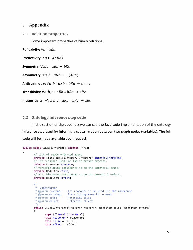
51
7 Appendix
7.1 Relation properties
Some important properties of binary relations:
Reflexivity:
Irreflexivity:
Symmetry:
Asymmetry:
Antisymmetry:
Transitivity:
Intransitivity:
7.2 Ontology inference step code
In this section of the appendix we can see the Java code implementation of the ontology
inference step used for inferring a causal relation between two graph nodes (variables). The full
code will be made available upon request.
public class CausalInference extends Thread { // List of newly oriented edges. private List<Touple<Integer, Integer>> inferedDirections; // The reasoner used for the inference process. private Reasoner reasoner; // Variable being considered to be the potential cause. private NodeItem cause; // Variable being considered to be the potential effect. private NodeItem effect; /** * Constructor * @param reasoner The reasoner to be used for the inference * @param ontology The ontology name to be used * @param cause Potential cause * @param effect Potential effect */ public CausalInference(Reasoner reasoner, NodeItem cause, NodeItem effect) { super("Causal inference"); this.reasoner = reasoner; this.cause = cause; this.effect = effect;
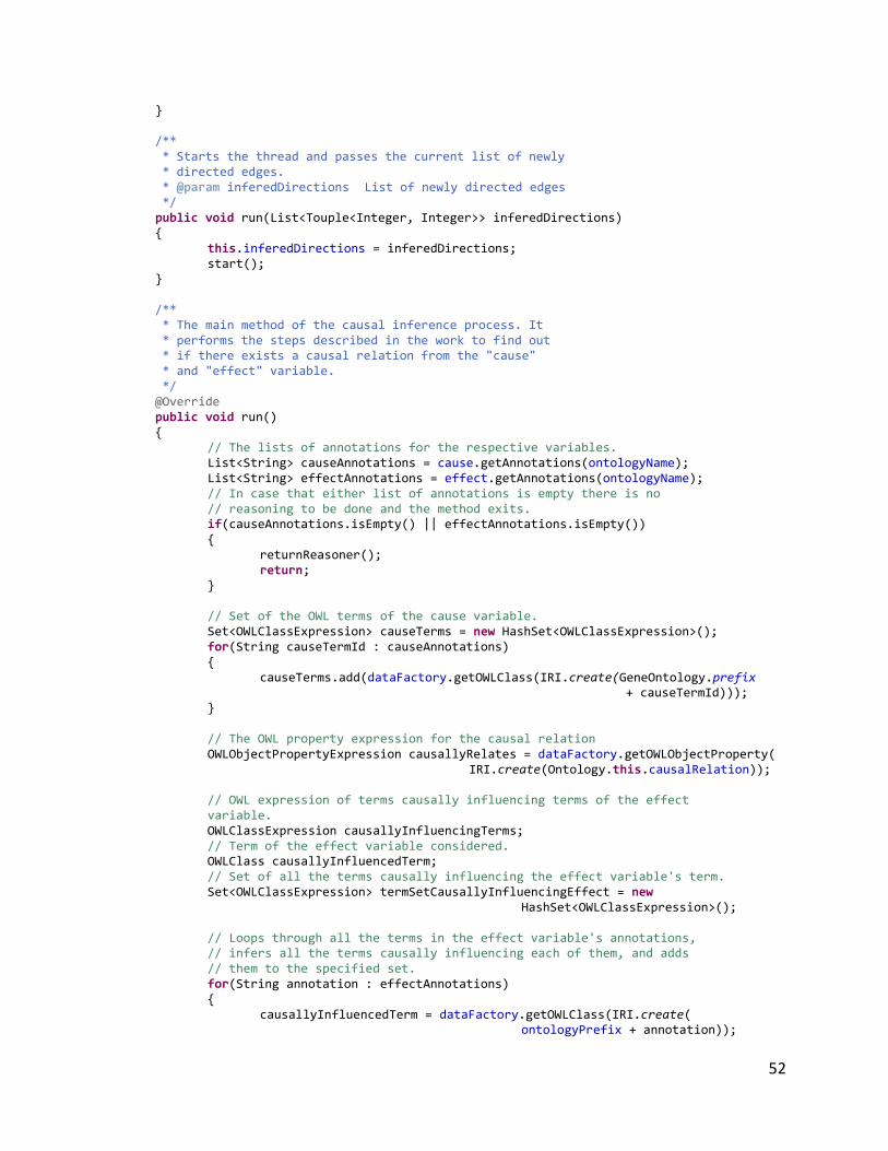
52
} /** * Starts the thread and passes the current list of newly * directed edges. * @param inferedDirections List of newly directed edges */ public void run(List<Touple<Integer, Integer>> inferedDirections) { this.inferedDirections = inferedDirections; start(); } /** * The main method of the causal inference process. It * performs the steps described in the work to find out * if there exists a causal relation from the "cause" * and "effect" variable. */ @Override public void run() { // The lists of annotations for the respective variables. List<String> causeAnnotations = cause.getAnnotations(ontologyName); List<String> effectAnnotations = effect.getAnnotations(ontologyName); // In case that either list of annotations is empty there is no // reasoning to be done and the method exits. if(causeAnnotations.isEmpty() || effectAnnotations.isEmpty()) { returnReasoner(); return; } // Set of the OWL terms of the cause variable. Set<OWLClassExpression> causeTerms = new HashSet<OWLClassExpression>(); for(String causeTermId : causeAnnotations)
{ causeTerms.add(dataFactory.getOWLClass(IRI.create(GeneOntology.prefix
+ causeTermId))); } // The OWL property expression for the causal relation
OWLObjectPropertyExpression causallyRelates = dataFactory.getOWLObjectProperty( IRI.create(Ontology.this.causalRelation));
// OWL expression of terms causally influencing terms of the effect
variable. OWLClassExpression causallyInfluencingTerms; // Term of the effect variable considered. OWLClass causallyInfluencedTerm; // Set of all the terms causally influencing the effect variable's term.
Set<OWLClassExpression> termSetCausallyInfluencingEffect = new HashSet<OWLClassExpression>();
// Loops through all the terms in the effect variable's annotations, // infers all the terms causally influencing each of them, and adds // them to the specified set. for(String annotation : effectAnnotations) { causallyInfluencedTerm = dataFactory.getOWLClass(IRI.create(
ontologyPrefix + annotation));
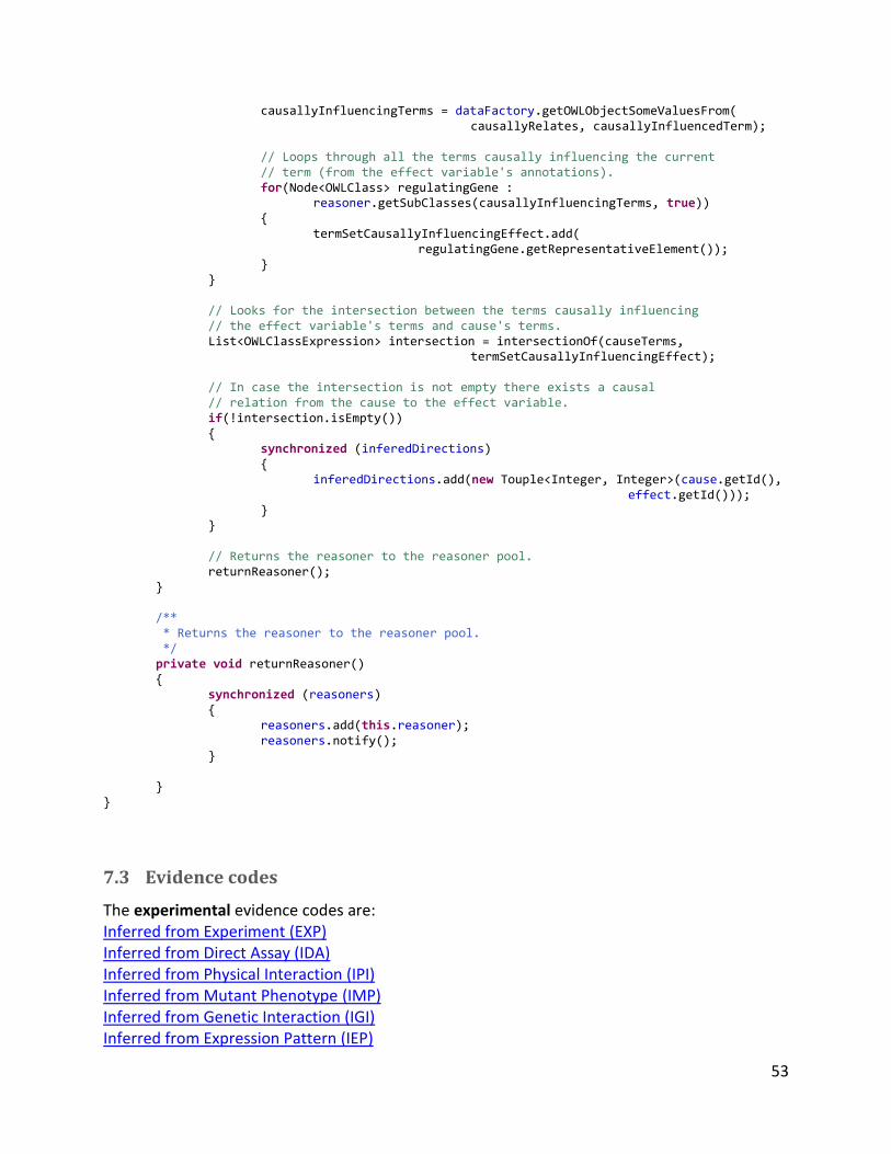
53
causallyInfluencingTerms = dataFactory.getOWLObjectSomeValuesFrom( causallyRelates, causallyInfluencedTerm);
// Loops through all the terms causally influencing the current // term (from the effect variable's annotations).
for(Node<OWLClass> regulatingGene : reasoner.getSubClasses(causallyInfluencingTerms, true))
{ termSetCausallyInfluencingEffect.add(
regulatingGene.getRepresentativeElement()); }
} // Looks for the intersection between the terms causally influencing // the effect variable's terms and cause's terms. List<OWLClassExpression> intersection = intersectionOf(causeTerms,
termSetCausallyInfluencingEffect); // In case the intersection is not empty there exists a causal // relation from the cause to the effect variable. if(!intersection.isEmpty()) { synchronized (inferedDirections) { inferedDirections.add(new Touple<Integer, Integer>(cause.getId(),
effect.getId())); } } // Returns the reasoner to the reasoner pool. returnReasoner(); } /** * Returns the reasoner to the reasoner pool. */ private void returnReasoner() { synchronized (reasoners) { reasoners.add(this.reasoner); reasoners.notify(); } } }
7.3 Evidence codes
The experimental evidence codes are: Inferred from Experiment (EXP) Inferred from Direct Assay (IDA) Inferred from Physical Interaction (IPI) Inferred from Mutant Phenotype (IMP) Inferred from Genetic Interaction (IGI) Inferred from Expression Pattern (IEP)
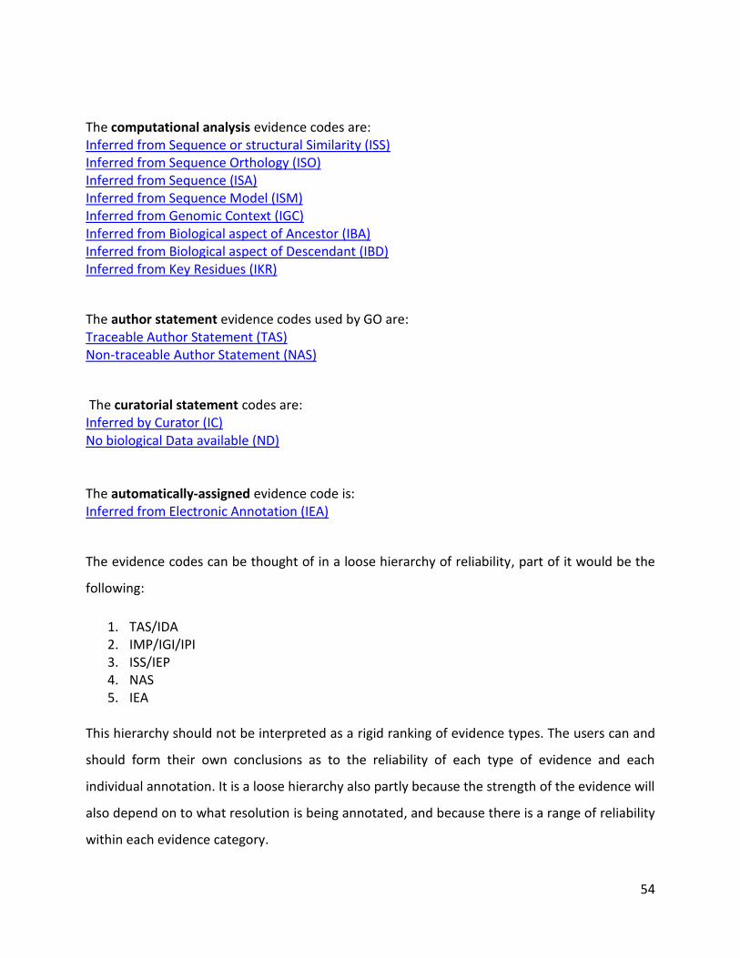
54
The computational analysis evidence codes are: Inferred from Sequence or structural Similarity (ISS) Inferred from Sequence Orthology (ISO) Inferred from Sequence (ISA) Inferred from Sequence Model (ISM) Inferred from Genomic Context (IGC) Inferred from Biological aspect of Ancestor (IBA) Inferred from Biological aspect of Descendant (IBD) Inferred from Key Residues (IKR)
The author statement evidence codes used by GO are: Traceable Author Statement (TAS) Non-traceable Author Statement (NAS)
The curatorial statement codes are: Inferred by Curator (IC) No biological Data available (ND) The automatically-assigned evidence code is: Inferred from Electronic Annotation (IEA)
The evidence codes can be thought of in a loose hierarchy of reliability, part of it would be the
following:
1. TAS/IDA 2. IMP/IGI/IPI 3. ISS/IEP 4. NAS 5. IEA
This hierarchy should not be interpreted as a rigid ranking of evidence types. The users can and
should form their own conclusions as to the reliability of each type of evidence and each
individual annotation. It is a loose hierarchy also partly because the strength of the evidence will
also depend on to what resolution is being annotated, and because there is a range of reliability
within each evidence category.
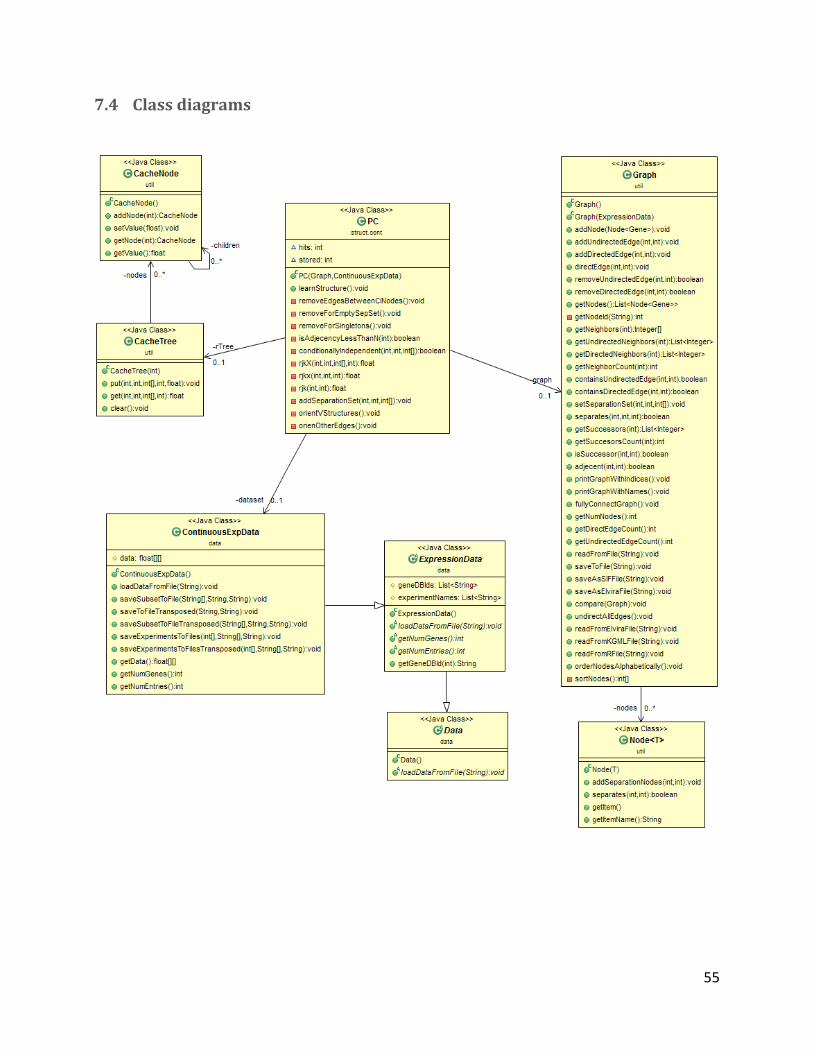
55
7.4 Class diagrams
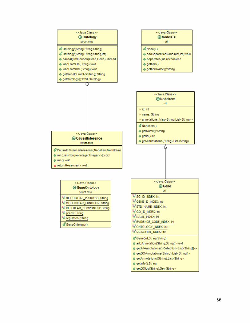
56
57
8 Bibliography
[1] -
Salcedo, J. (2004). A comparison of learning algorithms for Bayesian networks: a case study based on
data from an emergency medical service. Artificial Intelligence in Medicine, 30(3), 215-232.
[2] Al-Akwaa, F. M., & Alkhawlani, M. M. (2012). Comparison of the Bayesian Network Structure Learning
Algorithms. International Journal, 2(3).
[3] Alpaydin, E. (2004). Introduction to machine learning. MIT press.
[4] Ashburner, M., Ball, C. A., Blake, J. A., Botstein, D., Butler, H., Cherry, J. M., ... & Sherlock, G. (2000).
Gene Ontology: tool for the unification of biology.Nature genetics, 25(1), 25-29.
[5] Buntine, W. (1996). A guide to the literature on learning probabilistic networks from data. Knowledge
and Data Engineering, IEEE Transactions on, 8(2), 195-210.
[6] Carvalho, A. M. (2009). Scoring functions for learning bayesian networks. Inesc-id Tec. Rep.
[7] Chen, X. W., Anantha, G., & Wang, X. (2006). An effective structure learning method for constructing
gene networks. Bioinformatics, 22(11), 1367-1374.
[8] Cheng, J., Bell, D., & Liu, W. (1998). Learning Bayesian networks from data: An efficient approach
based on information theory. On World Wide Web at http://www.cs.ualberta.ca/~jcheng/bnpc.htm.
[9] Cooper, G. F., & Yoo, C. (1999). Causal discovery from a mixture of experimental and observational
data. In Proceedings of the Fifteenth conference on Uncertainty in artificial intelligence (pp. 116-125).
Morgan Kaufmann Publishers Inc..
[10] De Campos, C. P., Zeng, Z., & Ji, Q. (2009). Structure learning of Bayesian networks using
constraints. In Proceedings of the 26th Annual International Conference on Machine Learning (pp. 113-
120). ACM.
[11] De Jong, H. (2002). Modeling and simulation of genetic regulatory systems: a literature
review. Journal of computational biology, 9(1), 67-103.
[12] Dentler, K., Cornet, R., ten Teije, A., & de Keizer, N. (2011). Comparison of reasoners for large
ontologies in the OWL 2 EL profile. Semantic Web, 2(2), 71-87.
[13] Devitt, A., Danev, B., & Matusikova, K. (2006). Ontology-driven Automatic Construction of Bayesian
Networks for Telecommunication Network Management. In 2nd Int. Workshop: Formal Ontologies Meet
Industry (FOMI 2006).
[14] Ding, Z., Peng, Y., & Pan, R. (2006). BayesOWL: Uncertainty modeling in semantic web ontologies.
In Soft Computing in Ontologies and Semantic Web(pp. 3-29). Springer Berlin Heidelberg.
[15] Friedman, N., & Koller, D. (2000). Being Bayesian about network structure. In Proceedings of the
Sixteenth conference on Uncertainty in artificial intelligence (pp. 201-210). Morgan Kaufmann Publishers
Inc..
58
[16] Friedman, N., Linial, M., Nachman, I., & Pe'er, D. (2000). Using Bayesian networks to analyze
expression data. Journal of computational biology, 7(3-4), 601-620.
[17] Friedman, N., & Nachman, I. (2000). Gaussian process networks. InProceedings of the Sixteenth
conference on Uncertainty in artificial intelligence(pp. 211-219). Morgan Kaufmann Publishers Inc..
[18] Friedman, N. (2004). Inferring cellular networks using probabilistic graphical
models. Science, 303(5659), 799-805.
[19] Fu, L. D. (2005). A comparison of state-of-the-art algorithms for learning bayesian network structure
from continuous data.
[20] Goodman, N. D., Ullman, T. D., & Tenenbaum, J. B. (2011). Learning a theory of
causality. Psychological review, 118(1), 110.
[21] Harris, M. A., Clark, J., Ireland, A., Lomax, J., Ashburner, M., Foulger, R., ... & Gwinn, M. (2004). The
Gene Ontology (GO) database and informatics resource.Nucleic acids research, 32(Database issue),
D258-61.
[22] Hartemink, A. J., Gifford, D. K., Jaakkola, T., & Young, R. A. (2001). Using graphical models and
genomic expression data to statistically validate models of genetic regulatory networks. In Pacific
symposium on biocomputing(Vol. 6, No. 422-433, p. 266).
[23] Hartemink, A. J., Gifford, D. K., Jaakkola, T. S., & Young, R. A. (2002). Combining location and
expression data for principled discovery of genetic regulatory network models. In Proceedings of the
Pacific Symposium on Biocomputing (PSB’02) (pp. 437-449).
[24] Harwood, S., & Scheines, R. (2002). Genetic algorithm search over causal models.
[25] Heckerman, D. (1995). A Bayesian approach to learning causal networks. In Proceedings of the
Eleventh conference on Uncertainty in artificial intelligence (pp. 285-295). Morgan Kaufmann Publishers
Inc..
[26] Helsper, E. M., & van der Gaag, L. C. (2002). Building Bayesian networks through ontologies.
In ECAI (Vol. 2002, p. 15th).
[27] H y P O D j P t hölk f B (2009) N l l v y
with additive noise models.
[28] Ishak, M. B., Leray, P., & Amor, N. B. (2011). Ontology-based generation of object oriented Bayesian
networks. In Proceedings of the 8th Bayesian Modelling Applications Workshop (pp. 9-17).
[29] Jeon, B. J., & Ko, I. Y. (2007). Ontology-based semi-automatic construction of bayesian network
models for diagnosing diseases in e-health applications. In Frontiers in the Convergence of Bioscience
and Information Technologies, 2007. FBIT 2007 (pp. 595-602). IEEE.
[30] Kemp, C., Goodman, N. D., & Tenenbaum, J. B. (2007). Learning causal schemata. In Proceedings of
the 29th Annual Cognitive Science Society (pp. 389-394).
[31] Koller, D., & Friedman, N. (2009). Probabilistic graphical models: principles and techniques. The MIT
Press.
[32] Korb, K. B., & Nicholson, A. E. (2003). Bayesian artificial intelligence. CRC press.
59
[33] Lucas, C. G., & Griffiths, T. L. (2010). Learning the form of causal relationships using hierarchical
Bayesian models. Cognitive Science, 34(1), 113-147.
[34] Messaoud, M. B., Leray, P., & Amor, N. B. (2011). SemCaDo: a serendipitous strategy for learning
causal bayesian networks using ontologies. In Symbolic and Quantitative Approaches to Reasoning with
Uncertainty (pp. 182-193). Springer Berlin Heidelberg.
[35] Murphy, K. P. (2001). Active learning of causal Bayes net structure.
[36] Pazzani, M. (1991). A computational theory of learning causal relationships.Cognitive Science, 15(3),
401-424.
[37] Pe'er, D. (2003). From Gene Expression to Molecular Pathways (Doctoral dissertation, Hebrew
University of Jerusalem).
[38] Pearl, J., & Verma, T. S. (1995). A theory of inferred causation. Studies in Logic and the Foundations
of Mathematics, 134, 789-811.
[39] Pearl, J. (2000). Causality: models, reasoning and inference (Vol. 29). Cambridge: MIT press.
[40] Petri, N., Pekka, R., Tomi, S., & Henry, T. (2003). Investigating Non-linearities with Bayesian
Networks. management, 3(93), 81.
[41] Russell, S. J., Norvig, P., Canny, J. F., Malik, J. M., & Edwards, D. D. (1995).Artificial intelligence: a
modern approach (Vol. 74). Englewood Cliffs: Prentice hall.
[42] Sakamoto, Y., Ishiguro, M., & Kitagawa, G. (1986). Akaike information criterion statistics. Dordrecht,
The Netherlands: D. Reidel.
[43] Schwarz, G. (1978). Estimating the dimension of a model. The annals of statistics, 6(2), 461-464.
[44] Spellman, P. T., Sherlock, G., Zhang, M. Q., Iyer, V. R., Anders, K., Eisen, M. B., ... & Futcher, B.
(1998). Comprehensive identification of cell cycle–regulated genes of the yeast Saccharomyces
cerevisiae by microarray hybridization.Molecular biology of the cell, 9(12), 3273-3297.
[45] Spirtes, P., Glymour, C., & Scheines, R. (2000). Causation, prediction, and search (Vol. 81). The MIT
Press.
[46] Tenenbaum, J. B., & Niyogi, S. (2003). Learning causal laws. In Proceedings of the Twenty-Fifth
Annual Conference of the Cognitive Science Society.
[47] Tong, S., & Koller, D. (2001). Active learning for structure in Bayesian networks. In International joint
conference on artificial intelligence (Vol. 17, No. 1, pp. 863-869). LAWRENCE ERLBAUM ASSOCIATES
LTD.
[48] Troyanskaya, O., Cantor, M., Sherlock, G., Brown, P., Hastie, T., Tibshirani, R., ... & Altman, R. B.
(2001). Missing value estimation methods for DNA microarrays. Bioinformatics, 17(6), 520-525.
[49] Tsamardinos, I., Aliferis, C. F., Statnikov, A. R., & Statnikov, E. (2003). Algorithms for Large Scale
Markov Blanket Discovery. In FLAIRS Conference(Vol. 2003, pp. 376-381).
[50] Williamson, J. (2002). Learning causal relationships. London School of Economics, Centre for
Philosophy of Natural and Social Sciences.
60
[51] Yang, S., & Chang, K. C. (2002). Comparison of score metrics for Bayesian network
learning. Systems, Man and Cybernetics, Part A: Systems and Humans, IEEE Transactions on, 32(3),
419-428.
[52] Yehezkel, R., & Lerner, B. (2009). Bayesian network structure learning by recursive autonomy
identification. The Journal of Machine Learning Research,10, 1527-1570.
[53] Yu, J., Smith, V. A., Wang, P. P., Hartemink, A. J., & Jarvis, E. D. (2004). Advances to Bayesian
network inference for generating causal networks from observational biological
data. Bioinformatics, 20(18), 3594-3603.
[54] Zheng, H. T., Kang, B. Y., & Kim, H. G. (2008). An ontology-based bayesian network approach for
representing uncertainty in clinical practice guidelines. InUncertainty Reasoning for the Semantic Web
I (pp. 161-173). Springer Berlin Heidelberg.

61
9 Internet resources
[56] Bayes Nets. (2007, September 9). Retrieved June 10, 2013, from
http://www.bayesnets.com/
[57] Fisher transformation. (2013, June 7). In Wikipedia, The Free Encyclopedia. Retrieved May 5,
2013, from
http://en.wikipedia.org/w/index.php?title=Fisher_transformation&oldid=558763917
[58] Mutual information. (2013, June 12). In Wikipedia, The Free Encyclopedia. Retrieved 19:35, July 6,
2013, from http://en.wikipedia.org/w/index.php?title=Mutual_information&oldid=559501360
[59] Partial correlation. (2013, April 28). In Wikipedia, The Free Encyclopedia. Retrieved May 5,
2013, from http://en.wikipedia.org/w/index.php?title=Partial_correlation&oldid=552494794
[60] Pearson's chi-squared test. (2013, June 12). In Wikipedia, The Free Encyclopedia. Retrieved May 5,
2013, from http://en.wikipedia.org/w/index.php?title=Pearson%27s_chi-squared_test&oldid=559644550
[61] The Gene Ontology (2013). URL: http://www.geneontology.org
[62] Yeast Cell Cycle Analysis project. (2000, July 11). URL: http://genome-
www.stanford.edu/cellcycle/
[63] YeastMine. (2013, June 30). URL: http://yeastmine.yeastgenome.org/