Polar storms and polar jets: Mesoscale weather systems

in the Arctic & Antarctic

Ian Renfrew School of Environmental Sciences,

University of East Anglia

ECMWF-WWRP/Thorpex Polar Prediction Workshop – 24-27 June 2013

Outline

Introduction: global wind climatologies Mesoscale jets in the polar regions

Tip jets Barrier winds Katabatic winds Gap flows Polar foehn jets

Polar mesoscale cyclones

A global climatology of oceanic high wind speed events (> 20 m/s)

From: Sampe and Xie 2008 (BAMS): Mapping high sea winds from space – a global climatology

From: Sampe and Xie 2008 (BAMS): Mapping high sea winds from space – a global climatology

Top 4 stormiest places in world ocean have orographic influence All around 60-70 degrees N/S

• Tip Jets

• Barrier Winds

QuikSCAT climatology

Moore and Renfrew 2005, J. Climate

• Field programme: 17 Feb – 12 March 2007 • Detachment: Keflavik, Iceland • 62 flight hours + 9 hours (EUFAR)

From: Renfrew et al. 2008, Bulletin Amer Met Soc

From: Renfrew, Outten & Moore, 2009

Numerical Simulation: • Met Office UM 6.1 • 12 km grid & 76 levels • Initialised from Met

Office global analyses Configuration changes: • z0 over marginal ice zone

changed 100mm → 0.5mm

• z0 over sea ice changed 3mm → 0.5mm

• OSTIA high resolution SST & sea-ice field

Reasonably accurate

simulation: • 1-2 K and 2-3 m s-1 in ABL Renfrew, Outten and Moore, 2009: I Aircraft observations

Outten, Renfrew and Petersen, 2009: II Simulations and Dynamics + Erratum…

Numerical Simulation: • Met Office UM 6.1 • 12 km grid & 76 levels • Initialised from Met

Office global analyses Configuration changes: • z0 over marginal ice zone

changed 100mm → 0.5mm

• z0 over sea ice changed 3mm → 0.5mm

• OSTIA high resolution SST & sea-ice field

Reasonably accurate

simulation: • 1-2 K and 2-3 m s-1 in ABL Renfrew, Outten and Moore, 2009: I Aircraft observations

Outten, Renfrew and Petersen, 2009: II Simulations and Dynamics + Erratum…

What model

resolution is

required?

All 40L

From: DuVivier and Cassano, 2013, Mon Wea Rev, “Evaluation of WRF Model Resolution on Simulated Mesoscale Winds and Surface Fluxes near Greenland”

From: DuVivier and Cassano, 2013, Mon Wea Rev, “Evaluation of WRF Model Resolution on Simulated Mesoscale Winds and Surface Fluxes near Greenland”

ERAI BW climatology: Synoptic control

DSN

DSS: 238 events

DSN: 279 events

From Harden, Renfrew & Petersen 2011, J. Climate

ERAI Barrier Wind cross sections

DSS

DSN

ERAI - dashed Wind speed (thick) Potential temperature (thin)

Barrier Flows: 2 March

DS North Cross-section DS South Cross-section

Barrier Flows: 2 March Representation at 12 km grid, 76L is reasonable

DS South Cross-section

Impact of dropsonde data on Greenland coast

ORIGINAL DATASET (targeted sondes)

MODIFIED DATASET Replaced sondes on coast)

Dashed line = targeted solid line = all sondes dotted line = MODIFIED

See Irvine et al 2011, Mon Wea Rev

Barrier Winds in Antarctica

Nigro, Cassano, Lazzara & Keller, Mon Wea Rev, 2012

See also Schwerdtfeger 1975, MWR Parish 1983, JGR

Katabatic flows: Background

From Parish and Bromwich 1987, Nature

Locally driven “pure” katabatic flow Essentially Fb = (Δθ/θ0).g.α, where α = slope

•Validation from observed katabatic flows. • Conditionally sampled 6 < Umax < 8 m s-1 and 20 < zmax < 60 m

From Renfrew and Anderson (2006), Q. J. Royal Met. Soc.

0 1 2 3 4 5 6 7 8 9 100

20

40

60

80

100

120

140

160

180

200

Wind speed (m/s)

Hei

ght (

m)

0 1 2 3 4 5 6 7 8 9 10 0

20

40

60

80

100

120

140

160

180

200

Wind speed (m/s)

Hei

ght (

m)

MetUM Doppler sodar

Nightime comparison from summer-time case study – February 2002 MetUM at 4 km and 70L

RAMS idealised simulations

Summer case: wind

Barrier Flows, Tip Jets & Katabatic flows

• Synoptic situation and orography controls the jets location, timing and magnitude – As predictable as synoptic-scale flow – e.g. Barrier effect doubles peak wind speeds

• Resolution: ~10 km and 40-76 L seems necessary – MetUM simulations good (12 km & 76 L; 4 km for Katabatic) – WRF simulations good at 10 km, but 25 & 50 km grid size don’t

capture gradients – ERAI representation (80 km) ok for climatology, but similar

concerns about diffuse gradients • Parameterizations

– Sea-ice & SST fields and surface exchange vital – What can be done to capture sharp vertical gradients? – Poor representation of katabatic flows in vertical (SBL

parameterization problems?)

WEST EAST

Larsen

WEST EAST

Streamwise Wind (m/s)

Potential Temperature (K)

Vertical winds exaggerated (x25)

Foehn flows over Antarctic Peninsula Wave breaking Downslope windstorm Hydraulic jump

Larsen Ice Shelf

Larsen Ice Shelf

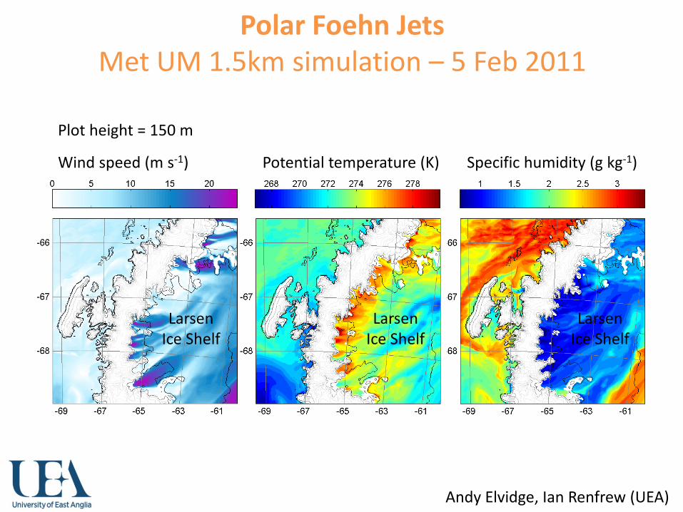
Potential temperature (K) Specific humidity (g kg-1) Wind speed (m s-1)

Polar Foehn Jets Met UM 1.5km simulation – 5 Feb 2011

Larsen Ice Shelf

Plot height = 150 m

Andy Elvidge, Ian Renfrew (UEA)

• 1.5 km grid size (76L) is required to simulate these polar foehn jets (gap flows).

• In addition surface exchange and BL parameterization is vital.

MetUM 1.5 km versus 4 km – 5 Feb 2011

Observations versus model

Andy Elvidge, Ian Renfrew (UEA)

• Left: along jet - shows warm föhn air reaching ice shelf with cold boundary layer to the east

• Below: across jet wind speed - shows model captures jet magnitude and approximate structure

OBS

MODEL

Met Office UM simulations at 1.5 km are able to capture most aspects of observed jet structure

Gap Flows, Polar foehn jets,

• Jets location and scale set by orography • Synoptic situation controls the jets timing and

magnitude – As predictable as synoptic-scale flow?

• Resolution: ~1 km and 76 L seems necessary – MetUM simulations good (at 1.5km & 76 L) – WRF simulations good at 1 km

• Parameterizations – Surface exchange vital – ABL parameterizations vital, e.g. SBL and BL transitions

Observations (1 km)

Regional model (10 km)

Global model (30 km)

Climate model (60 km)

What can atmospheric models resolve?

• Meteorological analyses (and climate models) have large amount of power “missing” in the atmospheric mesoscale • Does this matter for ocean circulation?

Along-track 10m wind speed spectra from QuikSCAT, ECMWF (dashed) and NCEP (thin) for the North Pacific in 2004. From Chelton et al. MWR, 2006

From Condron et al. 2006, Mon Wea Rev

Impact on deep convection in the

Greenland Sea

Impact on deep convection in the

Greenland Sea

Impact on subpolar gyre of the North Atlantic

Conclusions

• Appropriate model resolution is vital to resolve jets – ~10 km for larger-scale orographic jets – ~1 km for complex orography

• Appropriate parameterization schemes vital for accurate representation – SBL, surface exchange, etc

• Predictability seemingly controlled by synoptic-scales

B268 Easterly Tip Jet B271 Polar Low B273 Targeted SAP, Lee cyclogenesis & Barrier Winds B274 Barrier Winds

B275 Lee Cyclone

B276 Barrier Winds

B277 Barrier Winds

Barrier Flows: Temperature inversions

See Petersen, Renfrew and Moore, QJRMS, 2009

Numerical Simulations: RAMS

Numerical Simulations: RAMS at 3 km resolution

Potential temperature (K) Specific humidity (g kg-1) Wind speed (m s-1)

CI

WI

MOI

MOI = Mobil Oil Inlet WI = Whirlwind Inlet CI = Cabinet Inlet

Plot height = 150 m

Andy Elvidge, Ian Renfrew (UEA)

Met UM 1.5km simulation – 5 Feb 2011

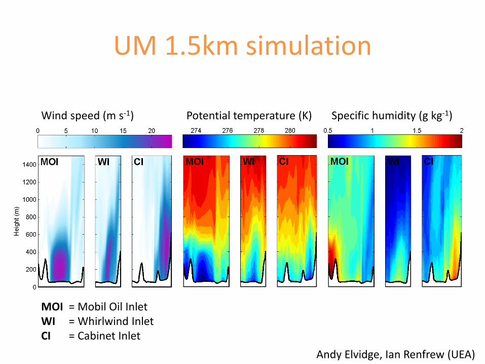
Potential temperature (K) Specific humidity (g kg-1) Wind speed (m s-1)

MOI WI CI

= Mobil Oil Inlet = Whirlwind Inlet = Cabinet Inlet

UM 1.5km simulation

Andy Elvidge, Ian Renfrew (UEA)