25february2012© 2012 The Royal Statistical Society

based on that fingerprint evidence would not have been brought based on the model. This was reassuring: it was a tough test, yet the method would in no case have helped to convict an innocent person. What of the reverse hypothesis? Fingerprint evidence is more usually used in court to help identify the guilty.

The North Wales crime-scene database was from cases that had been brought to court and successfully prosecuted; so the fingerprints from the true British-based perpetrators of the crimes were also available to compare to the traces. Here, too, the model performed satis-factorily. There is a clear separation between the likelihood ratios in the cases where print and mark came from the same person, and the cases where they came from different people. The more minutiae were used, the clearer was the separation.

The future

In the immediate future, we do not see that the current courtroom practice of presenting categorical opinions about fingerprints will change. But in the longer term we expect an evolution towards a framework that is similar to that which underpins DNA evidence. Already this work has formed the basis of training workshops in the UK, USA and in Europe. We have seen several years of courtroom battles in relation to DNA evidence. They have proved to be beneficial to the science. We must expect similar battles over this method. But the notion of a quantitative measure of the strength or weakness of evidence involves subtle issues which many lawyers fail to understand. It remains to be seen how future legal battles play out, but we see models such as this one as a powerful platform for change.

References1. Neumann, C., Mateos-Garcia, I.,

Langenburg, G., Kostroski, J., Skerrett, J.E. and Koolen, M. (2011) Operational benefits and challenges of the use of fingerprint statistical models: a field study. Forensic Science International, 212, 32–46.

2. Neumann, C., Evett, I.W. and Skerrett, J. (2012) Quantifying the weight of evidence assigned to a forensic fingerprint comparison: a new paradigm. Journal of the Royal Statistical Society, Series A, 175, 1–26.

Cedric Neumann is currently an Assistant Professor in Statistics at Pennsylvania State University. Cedric obtained his Ph.D. in Forensic Science from the oldest forensic programme in the world at the University of Lausanne, Switzerland. He has worked on forensic projects for the United States Secret Service and has managed a research team at the Forensic Science Service in the UK.

Playing the lottery with a little bit of stats know-how...Ian McHale dreams of winning the lottery. As a statistician, does he stand a better chance? With Rose D. Baker, he explains…

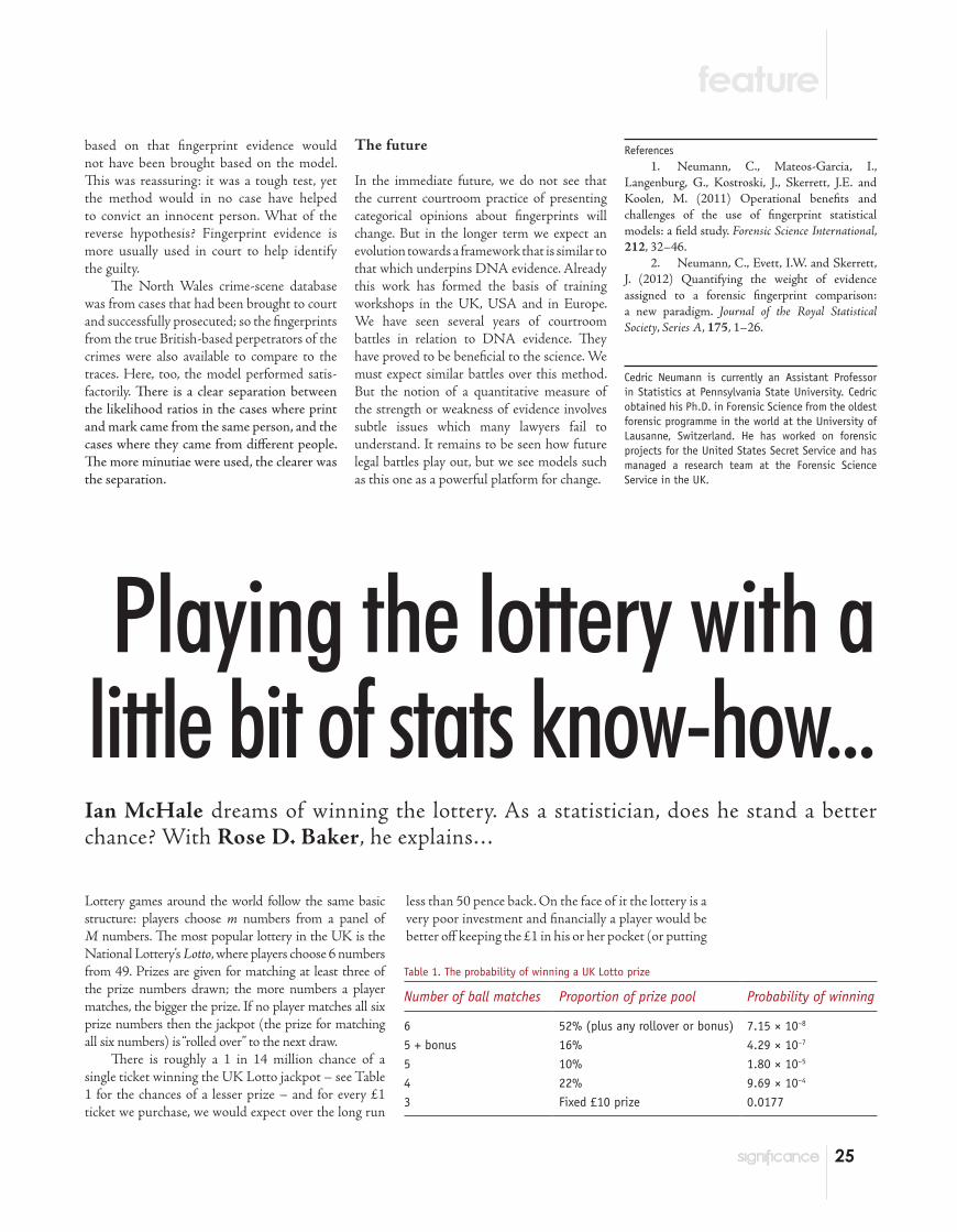
Lottery games around the world follow the same basic structure: players choose m numbers from a panel of M numbers. The most popular lottery in the UK is the National Lottery’s Lotto, where players choose 6 numbers from 49. Prizes are given for matching at least three of the prize numbers drawn; the more numbers a player matches, the bigger the prize. If no player matches all six prize numbers then the jackpot (the prize for matching all six numbers) is “rolled over” to the next draw.

There is roughly a 1 in 14 million chance of a single ticket winning the UK Lotto jackpot – see Table 1 for the chances of a lesser prize – and for every £1 ticket we purchase, we would expect over the long run

less than 50 pence back. On the face of it the lottery is a very poor investment and financially a player would be better off keeping the £1 in his or her pocket (or putting

Table 1. The probability of winning a UK Lotto prize

Number of ball matches Proportion of prize pool Probability of winning

6 52% (plus any rollover or bonus) 7.15 × 10–8

5 + bonus 16% 4.29 × 10–7

5 10% 1.80 × 10–5

4 22% 9.69 × 10–4

3 Fixed £10 prize 0.0177

25

26 february2012

it in the bank at even the meanest of interest rates). It might seem especially silly for any-body who has a grasp of probability to play. It begs the question: why do so many people play? One explanation offered by economists is that we are paying for the “dream”. What other way is there of being in with a chance

of getting a few million pounds added to your bank account? One of the authors plays the lottery (Ian’s fiancée actually buys the tickets – it is not the sort of thing a statistician should be seen doing himself ), and can confirm that he thoroughly enjoys the conversation over dinner on Saturday discussing what we would do if we won.

As statisticians, can we deduce anything about the lottery that may not be commonly known? Can statisticians gain an edge? Well, we cannot increase the probability of winning a prize as this is fixed. However, we can increase the amount we can expect to win if we do strike lucky – the “expected value” of the ticket we buy. The key to gaining this advantage is the existence of “conscious selection”.

What is conscious selection?

Conscious selection, a term that was first used by Cook and Clotfelter1, refers to any tendency of lottery players to pick their numbers non-randomly. For example, if players tend to pick birthdays, then numbers above 31 will be underrepresented. Alternatively, if players pick lucky numbers that they have in common – 7, for example, is a lucky number in many cultures – then those lucky numbers will be overrepresented. Those are just two of many mechanisms that can plausibly lead to conscious selection.

We can exploit the consequences of con-scious selection to increase the expected value of the tickets we buy. To see how, imagine two lottery players among many: player A picks

a popular combination of numbers, whilst player B chooses an unpopular combination. Both players have an equal probability of win-ning a prize. If player A is lucky enough to win the jackpot he may have to share his prize with other players, whilst if player B wins she may well be the sole winner and keep all of the money herself. In other words, choosing popular combinations of numbers decreases the expected value of your ticket as you have a higher probability of having to share your prize if you win.

The financial implications of choosing popular versus unpopular numbers can be large. In the early years of the UK Lotto, sales were typically 65 million and if players chose numbers randomly the expected number of jackpot winners would have been 4.65, with a standard deviation of 2.16. Yet on 14th Janu-ary 1995 there were an incredible 133 winners of the jackpot prize! On that occasion the win-ning numbers formed a zigzag pattern on the entry form – the numbers were 7, 17, 23, 32, 38 and 42, with bonus ball 48 – and it appears that many players choose numbers on the basis of forming familiar shapes – providing yet an-other mechanism for conscious selection. Had there been a single winner on that occasion rather than 133, he or she would have won £16 million. As it was, the winners got only £122 510 apiece – pleasant enough, but not quite so life-changing.

Another remarkable example of conscious selection comes from the Canadian lottery on 19th March 2008, when the six winning num-bers were 23, 40, 41, 42, 44 and 45 with bonus number 43. On that occasion there were no jackpot winners, but of the 6 606 690 tickets sold there were 239 winners of the prize for matching five numbers and the bonus number. If players were to choose numbers randomly the expected number of winners would be only 2.83 with a standard deviation of 1.68. Clearly many players chose the 40, 41, 42, 43, 44, 45 combination. Despite the negative but somewhat intuitive consequence of choosing popular combinations, lottery players continue to do so.

In South Africa, on 3rd March 2007, the organizing body of the lottery was forced to postpone future draws because political parties called for an investigation into the “extremely suspect” draw in which there were nine jack-pot winners. However, with conscious selec-tion, the occurrence of nine jackpot winners would not be unduly improbable. Evidence

of conscious selection seems to come from all around the world.

One consequence of conscious selection is that it leads to more rollovers. It is easy to see why. If more players than average choose “favourite” combinations, it follows that fewer players than average will choose the unpopular combinations; and if the prize numbers this week happen to form an unpopular combina-tion it may well be that no player has selected that combination, so there will be a rollover. Rollovers lead to larger jackpots and a more exciting game that attracts more players – so the mere existence of conscious selection is useful to lottery designers.

Indeed the simplest practicable way to scientifically detect conscious selection is to exploit its effect on rollovers. (A simpler way would be to look at the numbers selected on lottery tickets that have been sold, but lottery companies hate to release this data. As one re-searcher2 put it, lottery companies “guard this information like a poker player with a Royal Flush”.) We can look at the observed rate of rollovers and compare it to the theoretical probability of rollovers if there were no con-scious selection. For a probability, p, of winning the jackpot, and when Q tickets are sold, the rollover probability would be (1 – p)Q. How-ever, when players choose non-randomly, the coverage rate, which is defined as the propor-tion of all possible combinations of numbers purchased, is less than would result from ran-dom selection. Scoggins3 models the rollover probability as (1 – p)α + bQ and estimates α and b using data from the Florida State Lottery. If there was no conscious selection, α would be zero and b would be one. This is not the case and Scoggins concludes that players were choosing numbers non-randomly. Applying this logic to the UK Lotto, the observed prob-ability of no one winning is 0.180, whereas for the fitted Poisson distribution the predicted probability of a rollover is 0.0999. The dif-ference between these numbers is evidence of conscious selection.

In addition to there being more rollovers, conscious selection also affects the variance of the number of winners of prizes. We have al-ready seen that when a popular combination is selected as the winning combination there can be many winners. It is also the case that there may be very few winners (or even no winners) when unpopular numbers are the winning combination. This is true for all prize levels. Some weeks there may be many winners; some

It might seem especially silly for anyone with a grasp of

probability to play the lottery. So why do so many play?

27february2012

weeks may have few; and conscious selection makes this effect larger than we would expect under random selection.

A statistician can gain an advantage over other players by targeting unpopular combina-tions of numbers (or even by selecting numbers randomly.) Such a strategy would mean the player is less likely to have to share any prize he or she did win, and so the expected value of the ticket will increase. So can we identify which combinations are unpopular? Well, let’s see how far we can get by modelling conscious selection.

Modelling conscious selection

There are two approaches to modelling conscious selection: the first models the way players choose numbers; whilst the second only models the distributions of the numbers of winners of each prize that result as a consequence of non-random number selection. This less ambitious approach was adopted in Baker and McHale (2009). That model fitted the data well, but had the disadvantage of being purely descriptive. Our current work follows the first approach.

If there were no conscious selection, every number would stand the same chance of being chosen by a player, that chance being 1 in 49, or 0.0204. Farrell et al.4 assumed lottery

players had number preferences, such that players choose numbers with varying prob-abilities q1, q2,..., q49. Using their model (which has 48 parameters – the probability that 49 is chosen is of course 1 minus the probabilities for all the remaining numbers), we worked

out what those preferences might actually be. We have said that lottery companies will not divulge sales and number selections; but they inadvertently release a little of that data when they publish each week’s winning combina-tions and the number of people who share in the wins.

We used this with the statistical tech-nique of maximum likelihood to identify numbers that are unpopular5. Our estimated probabilities and the error bars for UK Lotto data under this model are plotted in Figure 1.

If all numbers were equally popular, the probability of each being selected would be 0.0204. Figure 1 shows that this is not the case, with the least popular numbers being 36, 37, 41, 45, 46 and 47. A lottery player could possibly increase the expected value of their ticket by selecting these numbers. Perhaps surprisingly, 13 is not among them.

There is, though, a catch. These are the most unpopular numbers. It does not follow that together they are the most unpopular combination.

Furthermore, the Farrell model does not actually fit the observed data very well. When popular numbers are drawn, there are many jackpot winners but also many winners of the lesser prizes. The Farrell model on its own does not produce these observed correlations.

Figure 1. Number preference probabilities and standard errors estimated from a maximum likelihood fit to sales and winnings numbers

Figure 2. The combination preference distribution model from equation (1), with parameters fitted to UK lottery data

0.014

0.016

0.018

0.02

0.022

0.024

0.026

0.028

0.03

0 10 20 30 40 50

Pro

babi

lity

Ball Number

0 2 4 6 8 10 12 14

Fre

quen

cy

Combination number (millions)

28 february2012

Measuring conscious selection

Recently we presented a model of conscious selection that allows not for number preferences, but for combination preferences, i.e. players having preferences for some of the 13 983 816 possible combinations6. To fit the equivalent of the Farrell et al. model would require a model with 13 983 815 parameters. This is clearly not possible. We therefore adopted the following approach. First, we listed the 14 million combinations in lexicographic order – that is, a numerical equivalent to an alphabetical order. Second, we imposed a probability distribution on to the list of combinations such that players choose each combination with varying probability. We do not need to know the actual preferred combinations; we just model the existence of groups of similar combinations, occurring with varying probabilities. Finally, we estimated the parameters of the probability distribution so as to maximise the likelihood of observing the number of winners of each of the different levels of prizes over many draws. This all requires some heroic computing! Again, much of this effort could have been avoided if lottery companies would disclose the data set of numbers selected by players.

The model we ended up with looked like Figure 2. It is actually an exponential probabil-ity distribution mixed with a uniform one and then tampered with. The up-and-down shape is because of our tampering: we chopped up the graph into segments of equal length and re-arranged them. The result is a “sawtooth” shape where neighbouring combinations of numbers can be either popular (chosen frequently) or unpopular (chosen infrequently.) The U-shape is an irrelevant accident of our tampering; what is important is that the model shows clusters of combinations that have a high probability of being selected by a player next to other clusters with low probability of being chosen.

The equation that gave rise to our graph, before we chopped it up, was

Pi = {(1 – f)(l exp(–l(i – 1)/Nc))/ (1 – exp(–l)) + f }/Nc (1)

where Pi is the probability of choosing the ith combination and Nc is the total number of combinations, which, as we have seen, is 13 983 816. f and l are parameters to be estimated.

Those parameters have an intuitive interpretation. l is a measure of the extent

of conscious selection for those players who practice it; when l = 0 there is no conscious selection. A proportion f of players choose numbers randomly, and the remainder choose from an exponential distribution. The use of f is reasonable, as it is known that some players do choose numbers randomly; for instance, some choose numbers using a random number generator provided by the lottery operator (“Lucky Dip”). The extent of conscious selection increases if f decreases or l increases.

Using this model, we can measure con-scious selection over time or across different countries. We obtained data from the UK’s Lotto game and from Spain’s El Gordo game. First, we compared the differences between the two. The values of l and f are slightly higher for the Spanish data than for the UK data. This suggests that a higher proportion of play-ers choose numbers randomly in Spain, but of those who choose non-randomly the degree of conscious selection is slightly higher than in the UK.

Rational players might learn over time to choose less popular numbers. A simple test for this is to look at the parameter estimates as they vary over time. We split the UK Lotto data into three equal time periods. We find that the parameter f increases slightly over time, but the increase is not statistically significant. Hence, the evidence suggests that lottery players in the UK have not learned to choose numbers randomly (let alone to choose unpopular numbers).

So what have we learnt?

Gaining an edge is really an aside of our model. The more serious reason to model conscious selection is that we hope it will aid lottery game designers to develop attractive games which generate higher revenues for good causes. Economists model sales of different lotteries using the mean, variance and skewness of the lottery ticket value. We have seen that conscious selection changes the expected value of the ticket; it changes the variance and skewness even more. Thus, to estimate models that predict sales correctly it is important to properly account for conscious selection.

The six least popular numbers are 36, 37, 41, 45, 46 and 49. A player wishing to maxim-ise their expected value could do worse than to choose these numbers. However, we first pub-lished this result in 20095, so these numbers

may well be a lot more popular now, at least if people who read RSS journals also buy lots of lottery tickets!

Further, when you select your numbers, you may as well try to choose a less popular com-bination that might increase your expected value. Unfortunately, it is not possible to determine what exactly the unpopular combinations are: there is not enough data. We do not even know whether our unpopular numbers are part of them. Our model does not identify actual com-binations and their popularity, rather it replicates the mechanism by which conscious selection may come about. Perhaps the simplest strategy is to use the Lucky Dip facility to choose random combinations for you – and if really keen, reject combinations that “look popular”.

Good luck in your attempts at “conscious non-conscious selection”. And if you do not win, then at least enjoy the dream…

Acknowledgements

We would like to thank our colleague Profes-sor David Forrest for helpful discussions. The full paper on which this article is based is in Journal of the Royal Statistical Society, Series A, October 20116.

References1. Cook, P. J. and Clotfelter, C. T. (1993)

The peculiar scale economies of Lotto. American Economic Review, 83, 634–643.

2. Hague, J. (2003) Taking Chances: Winning with Probability. Oxford: Oxford University Press.

3. Scoggins, J. F. (1995) The Lotto and expected net revenue. National Tax Journal, 48, 61–70.

4. Farrell, L., Hartley, R., Lanot, G. and Walker, I. (2000) ‘The Demand for Lotto: the Role of Conscious Selection’. Journal of Business and Economic Statistics, 18, 228–241

5. Baker, R. D. and McHale, I. G. (2009) Modelling the probability distribution of prize winnings in the UK National Lottery: conse-quences of conscious selection. Journal of the Royal Statistical Society, Series A, 172, 813–834.

6. Baker, R. D. and McHale, I. G. (2011) Investigating the behavioural characteristics of lottery players using a combination preference model for conscious selection. Journal of the Royal Statistical Society, Series A, 174, 1071–1086. doi: 10.1111/j.1467-985X.2011.00693.x

Rose D. Baker is Professor of Statistics at the Univer-sity of Salford, where Dr Ian McHale is Senior Lecturer on Applied Statistics.