PLATE BENDING ANALAYSIS USING FINITE ELEMENT METHOD · PLATE BENDING ANALAYSIS USING FINITE ELEMENT METHOD ... CHAPTER 1 INTRODUCTION Finite element method has emerged as a very important

1

PLATE BENDING ANALAYSIS USING

FINITE ELEMENT METHOD

A Project Report

Submitted in partial fulfillment for award of degree of

BACHELOR OF TECHNOLOGY

IN

MECHANICAL ENGINEERING

by

N SUDHIR (108ME015)

Under the guidance of

Prof N. Kavi

Professor, Department of Mechanical Engineering

Department of Mechanical Engineering

National Institute of Technology

2012

2

CERTIFICATE

This is to certify that the thesis entitled, “Plate bending analysis using Finite element method”

submitted by Mr N.SUDHIR in partial fulfillment of the requirements for the award of Bachelor

of Technology Degree in Mechanical Engineering at the National Institute of Technology,

Rourkela (Deemed University) is an authentic work carried out by him under my supervision and

guidance.

To the best of my knowledge, the matter embodied in the thesis has not been submitted to any

other University / Institute for the award of any Degree or Diploma.

Date Prof.N.Kavi

Dept. of Mechanical Engineering


Rourkela - 769008

3

ACKNOWLEDGEMENT

I wish to express my profound gratitude and indebtedness to Prof. N. Kavi , Department of

Mechanical Engineering , National Institute of Technology, Rourkela for introducing the present

topic and for his inspiring guidance, constructive criticism and valuable suggestion throughout the

project work.

I am also thankful to Prof K.P.Maity, Head of Mechanical Engineering

Department, National Institute of Technology, Rourkela for his constant support and

encouragement. I am also grateful to Prof D.R.K Parhi and Prof S.K Sahoo for their help and

support.

Lastly my sincere thanks to all my friends who has patiently extended all sorts of help

for accomplishing this undertaking.

N SUDHIR

Department of Mechanical Engineering


Rourkela – 769008

4

ABSTRACT

In the modern day to day applications like in industries,ships,pressure vessels,and other structural

components plates and shells play a major role so its very important to study their deformations

and slopes under loads inorder to understand their behaviour and possible conditions of failure,

one of the important factors on which the bending depends is on the load conditions and the

support conditions.So in the present study different type of conditions of plate holding such as

fixed clamping and simply supported conditions and free boundary conditions are applied on the

rectangular plates and their deformations are plotted and verified with that of values obtained with

general public licensed software LISA.

5

INDEX

Serial no Topic Page no

1 Introduction 6

2 Methodology adopted in Finite element method 8

3 Steps to solve for deflection using lisa 14

4 Results 16

5 Conclusion and

Discussion

29

7 Appendix 30

8 References 40

6

CHAPTER 1

INTRODUCTION

Finite element method has emerged as a very important mathematical tool in engineering

applications because it can reduce a problem with infinite no of degrees to a finite degree problem

with the help of discretization which is done according to the problem .For a beam or rod the

discretization procedure divides the whole rod or beam in to no of small linear elements thus

helping to apply the basic governing equations on each and every element and since all the

elements being the part of the complete rod/beam all are related with the help of global stiffness

matrices and the boundary conditions are applied inorder to solve the whole matrix of equations

and get the values of the unknown values at each node. Similar is the case with the 2 dimensional

plates here the plate is discretized into rectangular elements and the boundary conditions are

analyzed to get the unknown values at the discretized nodes but the disadvantage with this is it is

only a numerical method it can only come close to the analytical value but cannot be equal to it on

the other hand the great advantage which comes with FEM is it can easily solve the complex

governing equations which are very difficult to solve analytically and takes very long time in

getting solved ,thus saving from huge losses to modern industries.All these favourable

advantages come at the low cost of little inaccuracy since it‟s a numerical method.

1.1 AIM OF THE PRESENT WORK

The aim of the present work is to develop a matlab program which can work without the

dependence upon the plate materials and the aspect ratio. The input should be the

geometric dimensions of the plate such as length ,breadth , thickness. and plate material data

such as Poisson‟s ratio and Young‟s modulus and plot the graphs of various details such as

deflection and slopes of the plate curvature and to verify it with the values that are obtained

form the general public licencesed software LISA.

7

1.2 LITERATURE REVIEW

Addidsu Gezahegn Semie[2] had worked on numerical modellling on thin plates and solved

the problem of plate bending with the finite element method and Kirchoff‟s thin plate

theory is applied and program is written in fortran and the results were compared with the

help of ansys and the fortran program was given as an open source code.The analysis was

carried out for simple supported plate with distributed load,concentrated load and

clamped/fixed edges plates for both distributed and concentrated load.

L.Belounar and M Guenfoud[1] worked on to develop a rectangular finite element based on

the strain approach for plate bending .This new strain based rectangular plate

element(SBRP) was then compared with the other plate elements such as DKTM,DSTM

,SBH8 and other type of elements for cantilever platewith edge moment and edge shear and

found that SBRP convergence rate is very rapid,and free from shear locking and can be

applied to thick and thin plates.

Jian-Gang Han, Wei-Xin Ren,Yih Huang[3] developed a wavelet-based stochastic finite

element method is applied for bending bending analysis of thin plates. This wavelet theory

was based on the notion that any signal function can be broken down a series of local basis

functions called wavelet.Bending of square thin plates by using the developed spine wavelet

thin plate element formulation and bending moments and central deflection are analyzed for

simply supported and fixed supported.The method can achieve a hign numerical accuracy

and is very fast converging in solving the stochastic problem of thin plate bending.

P.R.S Speare,K.O.Kemp[4] worked on making a simplified reissner theory for plate

bending. A theory is developed which includes transverse shear and direct stress effects, and

solutions to this theories obtained using finite difference method and localized Ritz method

and its application to sandwich plates is also done and results are obtained for case of

practical shear stiffness to bending stiffness ratios.

8

CHAPTER 2

METHODOLOGY

ADOPTED IN FINITE ELEMENT METHOD

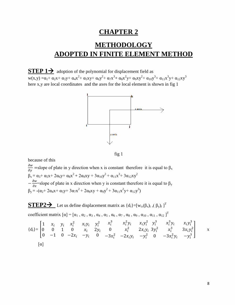
STEP 1 adoption of the polynomial for displacement field as

w(x,y) =α1+ α2x+ α3y+ α4x2+ α5xy+ α6y

2+ α7x

3+ α8x

2y+ α9xy

2+ α10y

3+ α11x

3y+ α12xy

3

here x,y are local coordinates and the axes for the local element is shown in fig 1

fig 1

because of this

slope of plate in y direction when x is constant therefore it is equal to βx

βx = α3+ α5x+ 2α6y+ α8x2 + 2α9xy + 3α10y

2 + α11x

3+ 3α12xy

2

=slope of plate in x direction when y is constant therefore it is equal to βy

βy = -(α2+ 2α4x+ α5y+ 3α7x2 + 2α8xy + α9y

2 + 3α11x

2y+ α12y

3)

STEP2 Let us define displacement matrix as {di}=[wi,(βx)i ,( βy)i ]T

coefficient matrix [α] = [α1 , α2 , α3 , α4 , α5 , α6 , α7 , α8 , α9 , α10 , α11 , α12 ]T

{di}= [

] x

[α]

9

STEP3 similarly {di ,dj ,dk ,dl }T =[A]

e x[α]

now strain matrix {ε}e ={

,

, -2

}

this gives

[A]=

[

]

now strain matrix is similarly

[ε]e =[

]x[α]

[ε]e=[H]x[α]

STEP4 now calculation of strain displacement matrix is done which is represented as [B]

this will be equal to for each element

[B] = [H] x[A]-1

now element stiffness matrix is calculated which is represented as [K]e

[K]e =∬

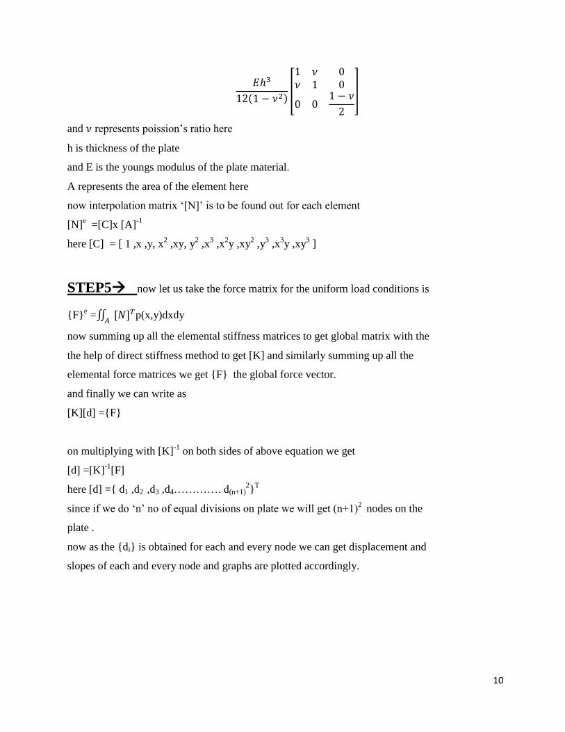
here [D] represents rigidity matrix which is equal to

10

( )[

]

and represents poission‟s ratio here

h is thickness of the plate

and E is the youngs modulus of the plate material.

A represents the area of the element here

now interpolation matrix „[N]‟ is to be found out for each element

[N]e =[C]x [A]

-1

here [C] = [ 1 ,x ,y, x2 ,xy, y

2 ,x

3 ,x

2y ,xy

2 ,y

3 ,x

3y ,xy

3 ]

STEP5 now let us take the force matrix for the uniform load conditions is

{F}e =∬

p(x,y)dxdy

now summing up all the elemental stiffness matrices to get global matrix with the

the help of direct stiffness method to get [K] and similarly summing up all the

elemental force matrices we get {F} the global force vector.

and finally we can write as

[K][d] ={F}

on multiplying with [K]-1

on both sides of above equation we get

[d] =[K]-1

[F]

here [d] ={ d1 ,d2 ,d3 ,d4…………. d(n+1)2}

T

since if we do „n‟ no of equal divisions on plate we will get (n+1)2

nodes on the

plate .

now as the {di} is obtained for each and every node we can get displacement and

slopes of each and every node and graphs are plotted accordingly.

11

DICRETIZATION

The discretization is done according to the following figure and if the no of divisions gets

increased it is done in the same manner. This dicretization is done for 64 elements.The node and

element number is shown accordingly.

fig 2

12

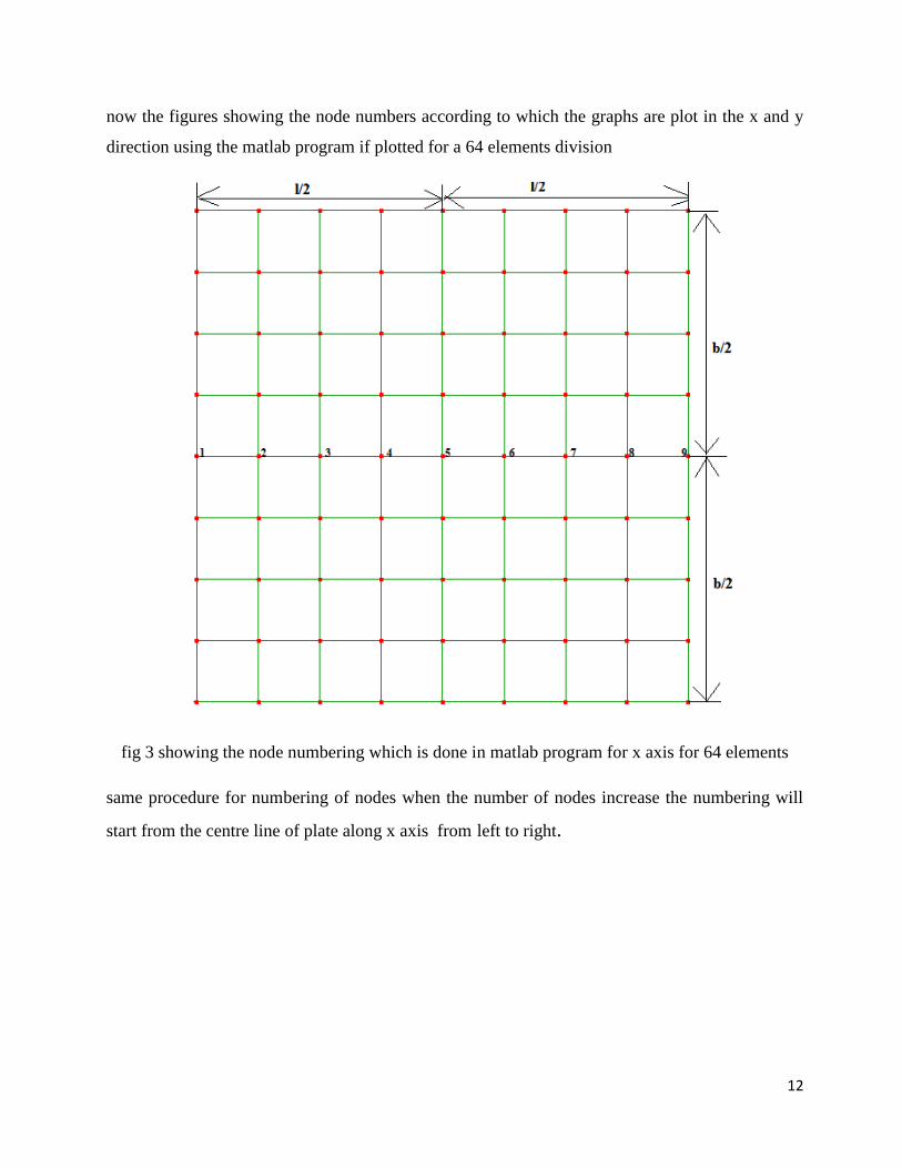
now the figures showing the node numbers according to which the graphs are plot in the x and y

direction using the matlab program if plotted for a 64 elements division

fig 3 showing the node numbering which is done in matlab program for x axis for 64 elements

same procedure for numbering of nodes when the number of nodes increase the numbering will

start from the centre line of plate along x axis from left to right.

13

fig 4 showing the node numbering which is done in matlab program for y axis for 64 elements

same procedure will follow in the no of elements increase node numbering will be done along the

centre line of the plate from the top to bottom

14

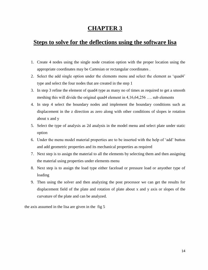
CHAPTER 3

Steps to solve for the deflections using the software lisa

1. Create 4 nodes using the single node creation option with the proper location using the

appropriate coordinates may be Cartesian or rectangular coordinates .

2. Select the add single option under the elements menu and select the element as „quad4‟

type and select the four nodes that are created in the step 1

3. In step 3 refine the element of quad4 type as many no of times as required to get a smooth

meshing this will divide the original quad4 element in 4,16,64,256 …. sub elements

4. In step 4 select the boundary nodes and implement the boundary conditions such as

displacement in the z direction as zero along with other conditions of slopes ie rotation

about x and y

5. Select the type of analysis as 2d analysis in the model menu and select plate under static

option

6. Under the menu model material properties are to be inserted with the help of „add‟ button

and add geometric properties and its mechanical properties as required

7. Next step is to assign the material to all the elements by selecting them and then assigning

the material using properties under elements menu

8. Next step is to assign the load type either faceload or pressure load or anyother type of

loading

9. Then using the solver and then analyzing the post processor we can get the results for

displacement field of the plate and rotation of plate about x and y axis or slopes of the

curvature of the plate and can be analyzed.

the axis assumed in the lisa are given in the fig 5

15

fig 5

the axes in lisa and matlab program y axis are just opposite to each other so the rotation about x

axis will be exactly opposite.

16

CHAPTER 4

RESULTS

CASE 1 - Rectangular plate clamped from all sides

dimension of the plate is 3 x 2 m, plate material is steel so Young‟s modulus is 21 x 1010

Pa

and Poission‟s ratio of 0.3 , face load/pressure load is taken as 14x 104 Pa. and plate thickness is

0.025 m, No of plate elements is taken as 400.

fig 6

fig 7 fig 8

17

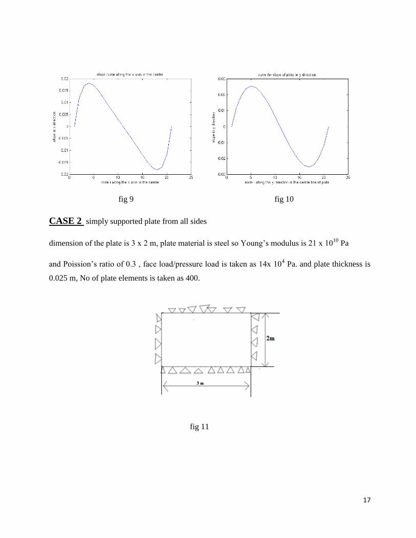
fig 9 fig 10

CASE 2 simply supported plate from all sides


Pa


0.025 m, No of plate elements is taken as 400.

fig 11

18

fig 12 fig 13

fig 14 fig 15

CASE 3 rectangular plate which is simply supported on y axis and clamped along the x axis


Pa


0.025 m, No of plate elements is taken as 400

19

fig 16

fig 17 fig 18

20

fig 19 fig 20

CASE 4 Rectangular plate which is clamped from two edges and free from the other two

edges . clamped along the x axis and free along the y axis.


Pa


0.025 m, No of plate elements is taken as 400

fig 21

21

fig 22 fig 23

fig 24 fig 25

22

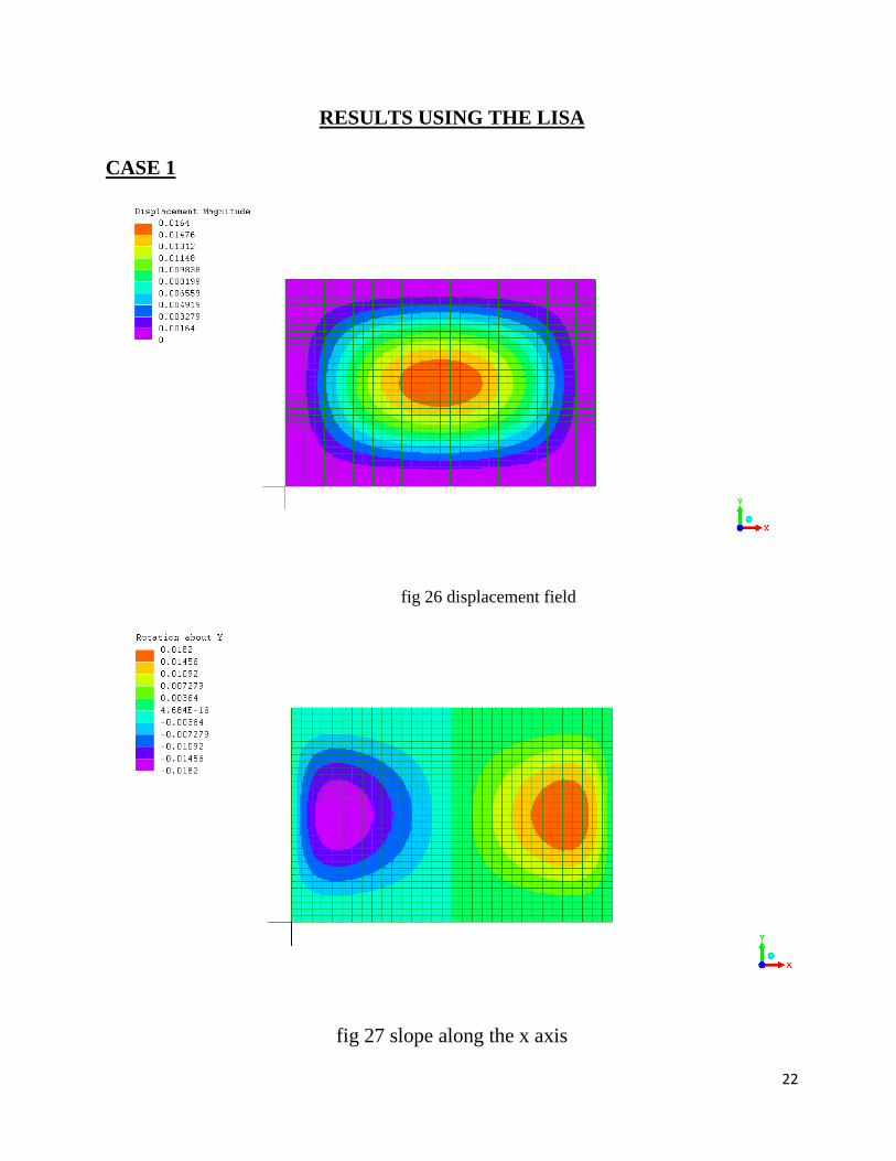
RESULTS USING THE LISA

CASE 1

fig 26 displacement field

fig 27 slope along the x axis

23

fig 28 slope along the y axis

CASE 2


24

fig 30 slope in the x direction

fig 31 slope in the y direction

25

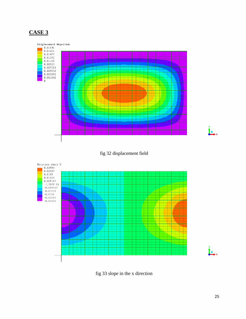
CASE 3


fig 33 slope in the x direction

26

fig 34 slope in y direction

CASE 4


27

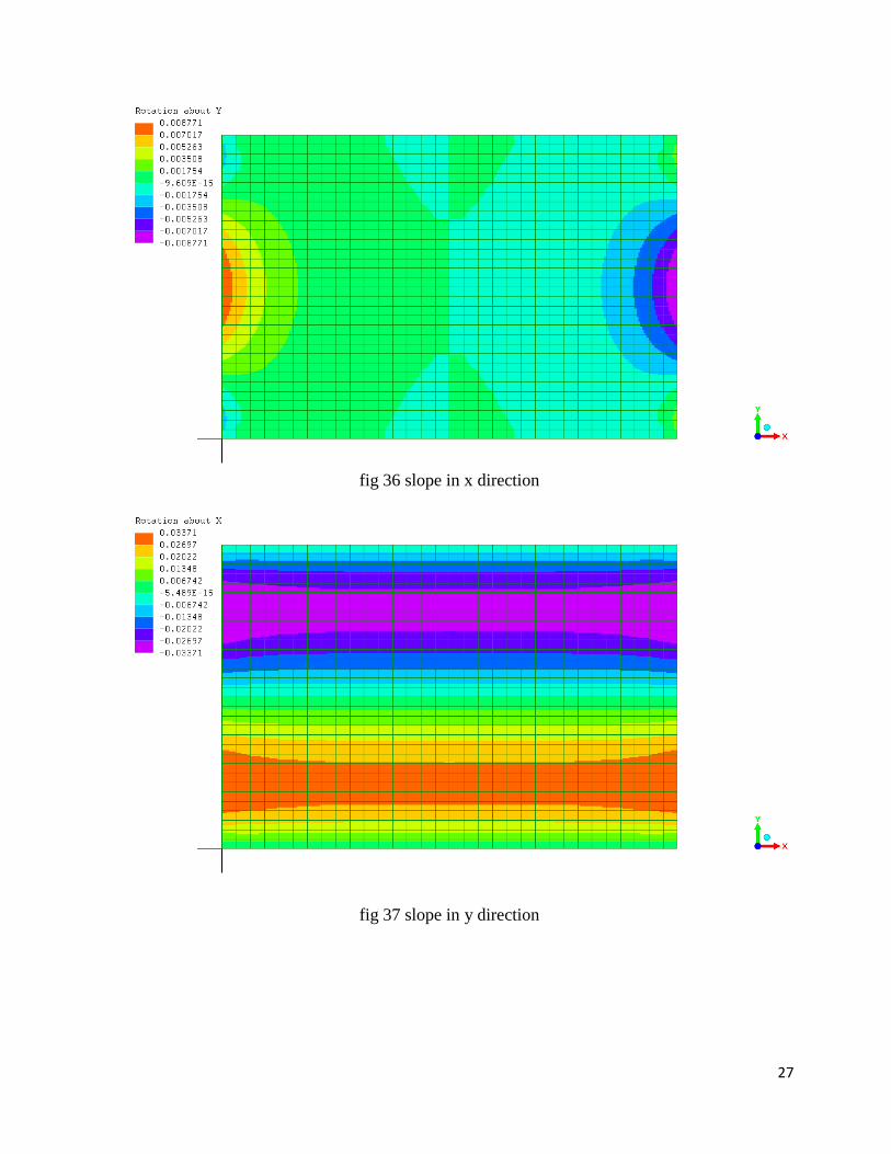
fig 36 slope in x direction

fig 37 slope in y direction

28

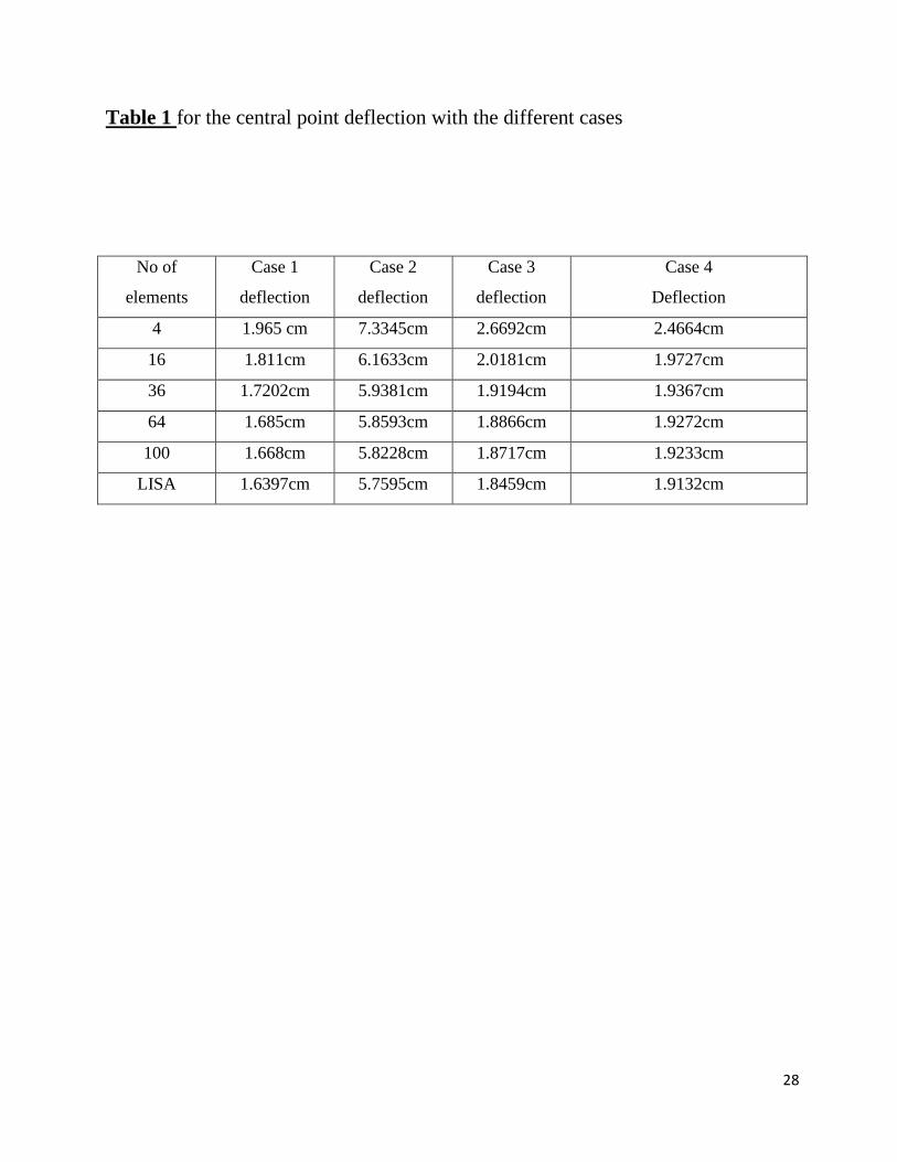
Table 1 for the central point deflection with the different cases

No of

elements

Case 1

deflection

Case 2

deflection

Case 3

deflection

Case 4

Deflection

4 1.965 cm 7.3345cm 2.6692cm 2.4664cm

16 1.811cm 6.1633cm 2.0181cm 1.9727cm

36 1.7202cm 5.9381cm 1.9194cm 1.9367cm

64 1.685cm 5.8593cm 1.8866cm 1.9272cm

100 1.668cm 5.8228cm 1.8717cm 1.9233cm

LISA 1.6397cm 5.7595cm 1.8459cm 1.9132cm

29

CHAPTER 5

CONCLUSION AND DISCUSSIONS

These problems that are encountered here are very common in nature we can easily find

structures having plates on which constant pressures (may be even for a small time interval but

constant )are applied such as the top plate of table,piston head,leaf valve,thin tin plate against fast

moving wind etc. We can see that due to symmetry we can easily predict that in a rectangular

plate that may be clamped from all edges,simply supported from all edges ,clamped and simply

supported etc. Maximum deflection is found to be at the centre of the plate in all cases and the

value of the deflection which are obtained from the finite element method using the Matlab

program is getting more and more accurate .Among the different conditions of clamping the

maximum deflection is obatined with the help of simply supported plates hence these type of

clampings are done to the plate in which deflection is acceptable and accordingly the fixed plates

are used where no deflection is needed. and rest other type of clampings are done in intermediate

requirements.And LISA colour coded deflection and slope fields can be easily visualized and can

give us the more details like bending moment about X and Y etc.and if presented code is

extended then again LISA can serve the purpose of comparing and crosschecking of the results.

Similarly bending moment and shear stresses are directly proportional to the rate of

change of slopes of slopes of the curvature of the deformed plate hence the steepness of the slope

graphs in X and Y direction indicates a stress value qualitatively

Since the present matlab code can be appended with the new and extra code without disturbing

the original code there is a scope to find out stresses, strains,analysis of plate with patch loading

conditions ,Bending moment ,shear forces,and analysis of skew plates,circular plates ,triangular

plates etc.

30

CHAPTER 6

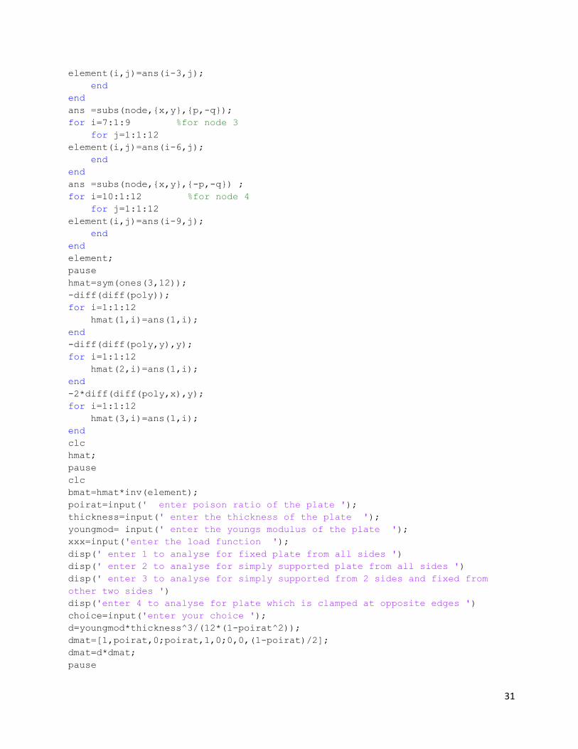
APPENDIX

clear

syms x y

poly=[1,x,y,x^2,x*y,y^2,x^3,x^2*y,x*y^2,y^3,x^3*y,x*y^3];

node=sym(ones(3,12));

element=sym(ones(12,12));

format shortEng

for i=1:1:12

node(1,i)=poly(1,i);

clc

end

diff(poly,y);

for i=1:1:12

node(2,i)=ans(1,i);

clc

end

-diff(poly,x);

for i=1:1:12

node(3,i)=ans(1,i);

clc

end

poly;

pause

clc

node;

pause

length=input(' enter the length of the plate ');

breadth=input(' enter the breadth of the plate ');

div=input(' enter the no of divisions on the length and breadth ');

p=length/(div*2);

q=breadth/(div*2);

ans =subs(node,{x,y},{-p,q});

pause on

pause

for i=1:1:3 %for node 1

for j=1:1:12

element(i,j)=ans(i,j);

end

end

ans=subs(node,{x,y},{p,q});


for j=1:1:12

31

element(i,j)=ans(i-3,j);

end

end

ans =subs(node,{x,y},{p,-q});


for j=1:1:12


end

end

ans =subs(node,{x,y},{-p,-q}) ;


for j=1:1:12


end

end

element;

pause

hmat=sym(ones(3,12));

-diff(diff(poly));

for i=1:1:12

hmat(1,i)=ans(1,i);

end

-diff(diff(poly,y),y);

for i=1:1:12

hmat(2,i)=ans(1,i);

end

-2*diff(diff(poly,x),y);

for i=1:1:12

hmat(3,i)=ans(1,i);

end

clc

hmat;

pause

clc

bmat=hmat*inv(element);

poirat=input(' enter poison ratio of the plate ');

thickness=input(' enter the thickness of the plate ');

youngmod= input(' enter the youngs modulus of the plate ');

xxx=input('enter the load function ');

disp(' enter 1 to analyse for fixed plate from all sides ')

disp(' enter 2 to analyse for simply supported plate from all sides ')

disp(' enter 3 to analyse for simply supported from 2 sides and fixed from

other two sides ')

disp('enter 4 to analyse for plate which is clamped at opposite edges ')

choice=input('enter your choice ');

d=youngmod*thickness^3/(12*(1-poirat^2));

dmat=[1,poirat,0;poirat,1,0;0,0,(1-poirat)/2];

dmat=d*dmat;

pause

32

clc

bmat'*dmat*bmat;

kmat=int((int (ans,x,-p,p)),y,-q,q);

kmat;

for i=1:1:12

for j=7:1:9

swap=kmat(i,j);

kmat(i,j)=kmat(i,j+3);

kmat(i,j+3)=swap;

end

end

for i=7:1:9

for j=1:1:12

swap=kmat(i,j);

kmat(i,j)=kmat(i+3,j);

kmat(i+3,j)=swap;

end

end

kmat;

pause

clc

globalmat=zeros((div+1)^2*3,(div+1)^2*3);

for i=1:1:div^2

for j=1:1:12

for k=1:1:12

quo=((i-1)-rem(i-1,div))/div;

if j<7

if k<7

globalmat(j+(i-1+quo)*3,k+(i-1+quo)*3)=globalmat(j+(i-

1+quo)*3,k+(i-1+quo)*3)+kmat(j,k);

else

globalmat(j+(i-1+quo)*3,k+(i-1+quo)*3+(div-

1)*3)=globalmat(j+(i-1+quo)*3,k+(i-1+quo)*3+(div-1)*3)+kmat(j,k);

end

else

if k<7

globalmat(j+(i-1+quo)*3+(div-1)*3,k+(i-

1+quo)*3)=globalmat(j+(i-1+quo)*3+(div-1)*3,k+(i-1+quo)*3)+kmat(j,k);

else

globalmat(j+(i-1+quo)*3+(div-1)*3,k+(i-1+quo)*3+(div-

1)*3)=globalmat(j+(i-1+quo)*3+(div-1)*3,k+(i-1+quo)*3+(div-1)*3)+kmat(j,k);

end

end

end

end

end

globalmat;

pause

clc

33

nmat=poly*inv(element);

qmat =int((int(nmat'*xxx,x,-p,p)),y,-q,q);

for i=7:1:9

swap=qmat(i,1);

qmat(i,1)=qmat(i+3,1);

qmat(i+3,1)=swap;

end

qmat

qmattotal=zeros((div+1)^2*3,1);

clc

quo=0;

for i=1:1:div^2

quo=((i-1)-rem(i-1,div))/div;

for j=1:1:12

if j<7

qmattotal(j+quo*3+(i-1)*3,1)=qmattotal(j+quo*3+(i-

1)*3,1)+qmat(j,1);

else

qmattotal(j+quo*3+(i-1)*3+(div-1)*3,1)=qmattotal(j+quo*3+(i-

1)*3+(div-1)*3,1)+qmat(j,1);

end

end

end

qmattotal;

b=10e20;

switch choice

case 1

for i=1:1:div+1 %modification of qmatrix

for j=1:1:3

qmattotal((i-1)*3+j,1)=0;

end

end

for i=(div+1)*div+1:1:(div+1)^2

for j=1:1:3


end

end

for i=1:(div+1):1+div*(div+1)

for j=1:1:3


end

end

for i=div+1:div+1:(div+1)^2

for j=1:1:3


end

end

for i=1:1:div+1 %modification of stiffness matrix

for j=1:1:3

34

globalmat((i-1)*3+j,(i-1)*3+j)=globalmat((i-1)*3+j,(i-1)*3+j)*b;

end

end


for j=1:1:3


end

end

for i=1+div+1:(div+1):1+(div-1)*(div+1)

for j=1:1:3


end

end

for i=(div+1)*2:div+1:(div+1)*div

for j=1:1:3


end

end

amat=zeros((div+1)^2*3,1);

amat=inv(globalmat)*qmattotal;

for i=1:1:3

disp(amat(((div+1)*(div/2)+(div/2))*3+i,1))

end

displacemat=zeros((div+1)^2,1);

slopey=zeros((div+1)^2,1);

slopex=zeros((div+1)^2,1);

for i=1:1:(div+1)^2

displacemat(i,1)=amat((i-1)*3+1);

slopey(i,1)=amat((i-1)*3+2);

slopex(i,1)=-amat((i-1)*3+3);

end

x=(div+1)*(div/2)+1:1:(div+1)*((div/2)+1);

y=displacemat(x,1);

plot(x-(div+1)*(div/2),y)

ylabel('deflection in x direction');

pause

x=(div+1)*(div/2)+1:1:(div+1)*((div/2)+1);

y=slopex(x,1);


ylabel('slope in x direction');

pause

x=((div+1)*div)+(div/2)+1:-(div+1):(div/2)+1;

y=displacemat(x,1);

x=1:1:div+1;

plot(x,y)

ylabel('deflection in y direction ');

pause


y=slopey(x,1);

35

x=1:1:div+1;

plot(x,y)

ylabel('slope in y direction ');

case 2


for j=1:2:3


end

end


for j=1:2:3


end

end


for j=1:1:2


end

end


for j=1:1:2


end

end


for j=1:2:3


end

end


for j=1:2:3


end

end


for j=1:1:2


end

end


for j=1:1:2


end

end



for i=1:1:3


end

36




for i=1:1:(div+1)^2




end

x=(div+1)*(div/2)+1:1:(div+1)*((div/2)+1);

y=displacemat(x,1);



pause

x=(div+1)*(div/2)+1:1:(div+1)*((div/2)+1);

y=slopex(x,1);



pause


y=displacemat(x,1);

x=1:1:div+1;

plot(x,y)


pause


y=slopey(x,1);

x=1:1:div+1;

plot(x,y)


case 3

disp('along the x axis plate is fixed and along y axis the plate is

simply supported')


for j=1:1:3


end

end


for j=1:1:3


end

end


for j=1:1:2


end

end


for j=1:1:2

37


end

end


for j=1:1:3


end

end


for j=1:1:3


end

end


for j=1:1:2


end

end


for j=1:1:2


end

end



for i=1:1:3


end




for i=1:1:(div+1)^2




end

x=(div+1)*(div/2)+1:1:(div+1)*((div/2)+1);

y=displacemat(x,1);



pause

x=(div+1)*(div/2)+1:1:(div+1)*((div/2)+1);

y=slopex(x,1);



pause


y=displacemat(x,1);

x=1:1:div+1;

38

plot(x,y)


pause


y=slopey(x,1);

x=1:1:div+1;

plot(x,y)


case 4

disp('the plate is clamped in both the x direction edges')

pause


for j=1:1:3


end

end


for j=1:1:3


end

end


for j=1:1:3


end

end


for j=1:1:3


end

end



for i=1:1:3


end




for i=1:1:(div+1)^2




end

x=(div+1)*(div/2)+1:1:(div+1)*((div/2)+1);

y=displacemat(x,1);



pause

39

x=(div+1)*(div/2)+1:1:(div+1)*((div/2)+1);

y=slopex(x,1);



pause


y=displacemat(x,1);

x=1:1:div+1;

plot(x,y)


pause


y=slopey(x,1);

x=1:1:div+1;

plot(x,y)

ylabel('slope in y direction ')

end

40

CHAPTER 7

REFERENCES

1. Belounar L.,Guenfoud M.,A new rectangular finite element based on the

strain approach for plate bending,Thin-walled structures,43,(2005),

pages47-63

2. Semie Addisu Gezahegn,Numerical modeling of thin plates using finite

element method,2010

3. Han Jian-Gang,Ren Wei-Xin,Huang Yih, A wavelet based stochastic finite

element method of thin plate bending, Applied mathematical

modeling,31,(2007),pages 181-193

4. Speare P.R.S,Kemp K.O.,A simplified Reissner theory for Plate

bending,International journal of solid structures,(1977),pp 1073-1079

5. Timoshenko Stephen S.,Krieger Woinowsky S,Theory of plates and shells

McGraw Hill,Singapore ,1959

6. Thompson Erik.G,Introduction to the finite element method theory

programming and applications,John wiley and sons(ASIA)Pte

Ltd,Singapore,2005

7. Shames Irving H.,DYM Clive L.,Energy and finite element methods in

structural mechanics,New age International ,New Delhi,2003

8. Krishnamoorthy C.S ,Finite element analysis,Theory and Programming,Tata

Mcgraw Hill,New Delhi,2010

41

Documents

PLATE BENDING ANALAYSIS USING FINITE ELEMENT METHOD · PLATE BENDING ANALAYSIS USING FINITE ELEMENT METHOD ... CHAPTER 1 INTRODUCTION Finite element method has emerged as a very important