Planarity testing of doubly periodic infinite graphs

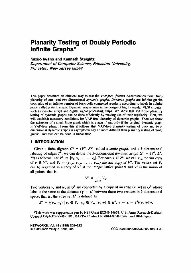
Planarity Testing of Doubly Periodic Infinite Graphs* Kazuo lwano and Kenneth Steiglitz Department of Computer Science, Princeton University, Princeton, New Jersey 08544

This paper describes an efficient way to test the VAP-free (Vertex Accumulation Point free) planarity of one- and two-dimensional dynamic graphs. Dynamic graphs are infinite graphs consisting of an infinite number of basic cells connected regularly according to labels in a finite graph called a sraric graph. Dynamic graphs arize in the design of highly regular VLSI circuits, such as systolic arrays and digital signal processing chips. We show that VAP-free planarity testing of dynamic graphs can be done efficiently by making use of their regularity. First, we will establish necessary conditions for VAP-free planarity of dynamic graphs. Then we show the existence of a small finite graph which is planar if and only if the original dynamic graph is VAP-free planar. From this it follows that VAP-free planarity testing of one- and two- dimensional dynamic graphs is asymptomically no more difficult than planarity testing of finite graphs, and thus can be done in linear time.

1. INTRODUCTION

Given a finite digraph Go = (V", Eo), called a static graph, and a k-dimensional labeling of edges P, we can define the k-dimensional dynamic graph Gk = (Vk, Ek, P) as follows: Let VO = { v l , vzr . . . , vn}. For each x E 2, we call vi,x the xrh copy of vi E V", and V, = {v,,,, vZ,,, . . . , v,,J the xrh copy of VO. The vertex set V , can be regarded as a copy of V" at the integer lattice point x and V is the union of all points; that is,

V = u v,. %€i?

Two vertices v, and wy in Gk are connected by a copy of an edge (v, w ) in Go whose label is the same as the distance (y - x) between these two vertices in k-dimensional space; that is. the edge set Ek is defined as

P = {(v,, wy) 1 v, E v,, wy E v y , (v, w ) E EO, y - x = PUv, w))}.

*This work was supported in part by NSF Grant ECS-8414674, U.S. A m y Research-Durham Contract DAAG29-85-K-0191, DARPA Contract N00014-82-K-0549, and IBM-Japan.

NETWORKS, Vol. 18 (1988) 205-222 0 1988 John Wiley B Sons, Inc. CCC 0028-3045/88/030205-1 s$o4.00

206 IWANO AND STElGLlTZ

( 0 . 0

( 0 . 0 )

A static graph GO

The dynamic graph GI

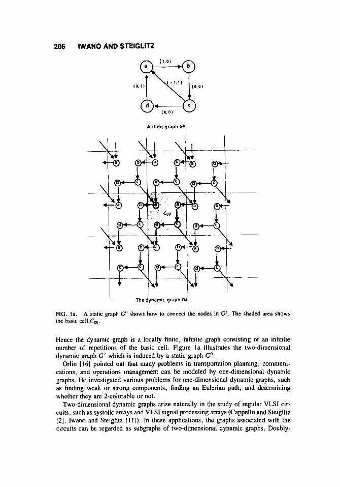
FIG. la. the basic cell C,.

A static graph e shows how to connect the nodes in GZ. The shaded area shows

Hence the dynamic graph is a locally finite, infinite graph consisting of an infinite number of repetitions of the basic cell. Figure la illustrates the two-dimensional dynamic graph G2 which is induced by a static graph GO.

Orlin [16j pointed out that many problems in transportation planning, communi- cations, and operations management can be modeled by one-dimensional dynamic graphs. He investigated various problems for one-dimensional dynamic graphs, such as finding weak or strong components, finding an Eulenan path, and determining whether they are 2-colorable or not.

Two-dimensional dynamic graphs arise naturally in the study of regular VLSI circuits, such as systolic arrays and VLSI signal processing arrays (Cappello and Steiglitz [2], Iwano and Steiglitz [ 1 I ] ) . In these applications, the graphs associated with the circuits can be regarded as subgraphs of two-dimensional dynamic graphs. Doubly-

PLANARITY TESTING 207

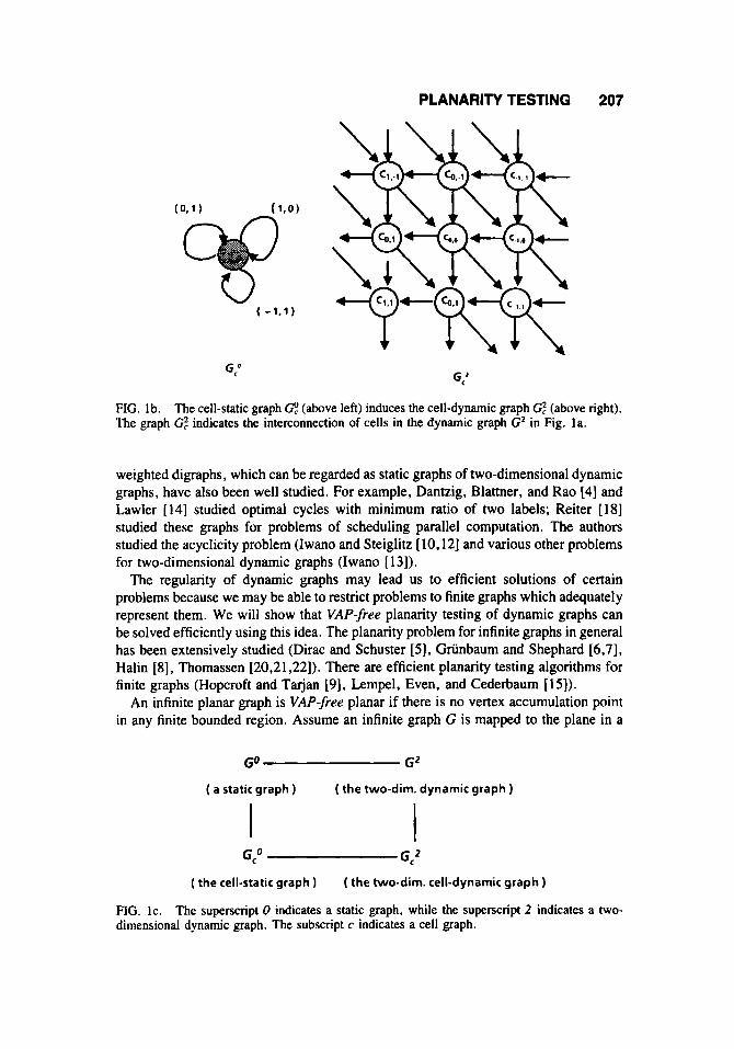
FIG. lb. The cell-static graph The graph Gf indicates the interconnection of cells in the dynamic graph G2 in Fig. la.

(above left) induces the cell-dynamic graph Gf (above right).

weighted digraphs, which can be regarded as static graphs of two-dimensional dynamic graphs, have also been well studied. For example, Dantzig, Blattner, and Rao [4] and Lawler [ 141 studied optimal cycles with minimum ratio of two labels; Reiter [ 181 studied these graphs for problems of scheduling parallel computation. The authors studied the acyclicity problem (Iwano and Steiglitz [ 10,121 and various other problems for two-dimensional dynamic graphs (Iwano [ 131).

The regularity of dynamic graphs may lead us to efficient solutions of certain problems because we may be able to restrict problems to finite graphs which adequately represent them. We will show that VAP-free planarity testing of dynamic graphs can be solved efficiently using this idea. The planarity problem for infinite graphs in general has been extensively studied (Dirac and Schuster [ 5 ] , Griinbaum and Shephard [6,7], Halin [8], Thomassen [20,21,22]). There are efficient planarity testing algorithms for finite graphs (Hopcroft and Tarjan [9], Lempel, Even, and Cederbaum [15]).

An infinite planar graph is VAP-free planar if there is no vertex accumulation point in any finite bounded region. Assume an infinite graph G is mapped to the plane in a

GO G2

( a static graph ) ( the two-dim. dynamic graph )

GC0 G,2 ( the cell-static graph ) ( the two-dim. cell-dynamic graph )

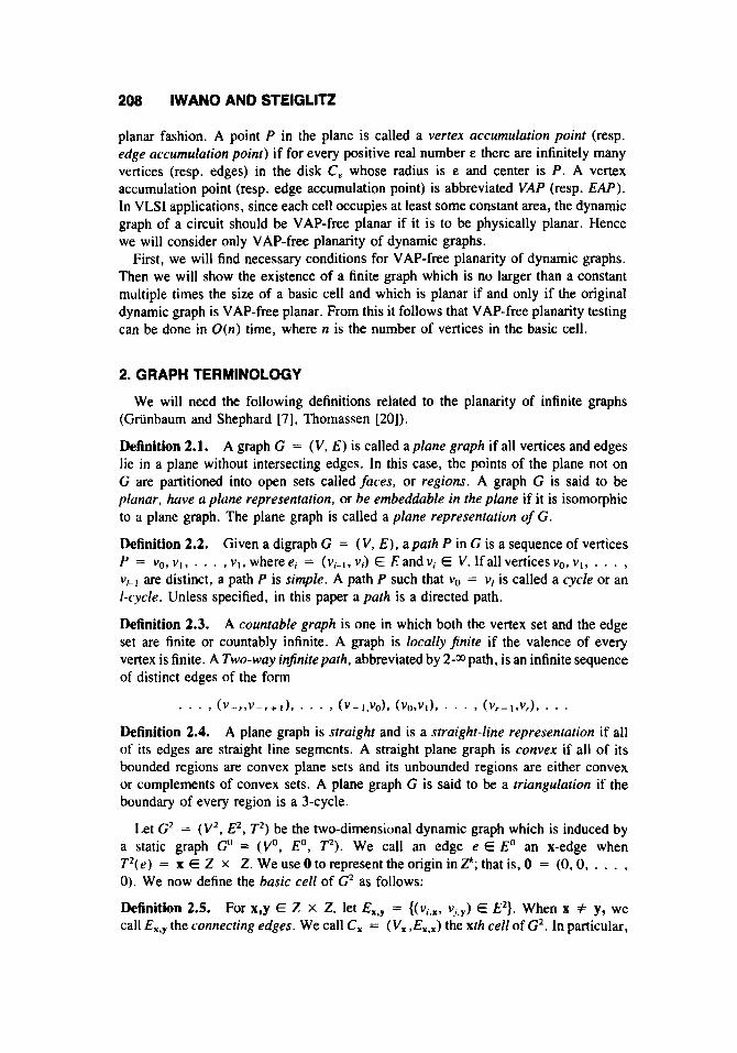
FIG. Ic. dimensional dynamic graph. The subscript c indicates a cell graph.

The superscript 0 indicates a static graph, while the superscript 2 indicates a two-


planar fashion. A point P in the plane is called a vertex accumulation point (resp. edge uccumulation point) if for every positive real number E there are infinitely many vertices (resp. edges) in the disk C, whose radius is E and center is P. A vertex accumulation point (resp. edge accumulation point) is abbreviated VAP (resp. E A P ) . In VLSl applications, since each cell occupies at least some constant area, the dynamic graph of a circuit should be VAP-free planar if it is to be physically planar. Hence we will consider only VAP-free planarity of dynamic graphs.

First, we will find necessary conditions for VAP-free planarity of dynamic graphs. Then we will show the existence of a finite graph which is no larger than a constant multiple times the size of a basic cell and which is planar if and only if the original dynamic graph is VAP-free planar. From this it follows that VAP-free planarity testing can be done in O ( n ) time, where n is the number of vertices in the basic cell.

2. GRAPH TERMINOLOGY

We will need the following definitions related to the planarity of infinite graphs (Griinbaum and Shephard [7], Thomassen [201).

Definition 2.1. A graph G = (V, E) is called a plane graph if all vertices and edges lie in a plane without intersecting edges. In this case, the points of the plane not on G are partitioned into open sets called faces, or regions. A graph G is said to be planar, have a plane representation, or be embeddable in the plane if it is isomorphic to a plane graph. The plane graph is called a plane representation of G.

Definition 2.2. Given a digraph G = ( V , E ) , apath P in G is a sequence of vertices P = v,, v l , . . . , v i , where el = (v i - , , vi) E E and vi E V. If all vertices vo, v l r . . . , v / - ~ are distinct, a path P is simple. A path P such that v, = vl is called a cycle or an I-cycle. Unless specified, in this paper a path is a directed path.

Definition 2.3. A countable graph is one in which both the vertex set and the edge set are finite or countably infinite. A graph is locallyfinite if the valence of every vertex is finite. A Two-way infinitepath, abbreviated by 2-a, path, is an infinite sequence of distinct edges of the form

v ( v - r , v - r + ~ ) v . * . 9 ( v - I . v o ) , (v09vl)r . . . 9 (vr-lvvr)v . . , Definition 2.4. A plane graph is straight and is a straight-line representation if all of its edges are straight line segments. A straight plane graph is convex if all of its bounded regions are convex plane sets and its unbounded regions are either convex or complements of convex sets. A plane graph G is said to be a triangulation if the boundary of every region is a 3-cycle.

Let G2 = ( V 2 , E 2 , T 2 ) be the two-dimensional dynamic graph which is induced by a static graph Go = (V", Eo, T2) . We call an edge e E Eo an x-edge when T 2 ( e ) = x E 2 x 2. We use 0 to represent the origin in 2'; that is, 0 = (0.0, . . . , 0). We now define the basic cell of G2 as follows:

Definition 2.5. For x,y E 2 X 2. let Ex,y = {(v,,, , Y ; . ~ ) E E2}. When x # y, we call EXqy the connecting edges. We call C, = ( V , ,Ex,,) the xth cell of G2. In particular,


we call C, the basic cell of Ck. When we regard each cell as a point, we have an infinite graph Gf = (V,’, Ef, Tf) such that Vf = Z X Z and E f = U,,, Ex,y. We call Gf the cell-dynamic graph of G2. A k-dimensional cell-dynamic graph is defined similarly. Figure lb illustrates a two-dimensional cell-dynamic graph G2.

The graph Gf is obtained by regarding every cell of Gz as a point; G2 can be regarded as the union of cells and connecting edges.

Definition 2.6. Let Gf = (e, Ef, c) be the cell-dynamic graph of a two-dimensional dynamic graph G2. Then we define the cell-static graph @ = (V:, E:, Tf) as follows :

v: = {v}

E: = {e = ( v , v ) I e E Ef, T ( e ) f 0) I Tf = { T Z ( e ) 1 e E E:}.

This cell-static graph c is the static graph which induces G:. In Figure la, the two-dimensional dynamic graph GZ is induced by the static graph Go, while in Figure lb, the cell-dynamic graph Gf is induced by the cell-static graph G!. The cell-dynamic graph Gf represents the interconnection between cells in the dynamic graph G2, and the cell-static graph consists of edges with non-0 labels in @. We use the notation illustrated in Figure lc. That is, a superscript 2 of G indicates a two-dimensional dynamic graph, while a superscript 0 indicates a static graph. A subscript c of C or G2 indicates a cell-dynamic graph.

From now on, we restrict discussion to one- and two-dimensional dynamic graphs.

Definition 2.7. To subdivide an edge e = (x, y) in a graph H, is to replace it by a new vertex 2. new edges e , = ( x , z) and e2 = ( 2 , y ) . We say that the resulting graph G is obtained from H by subdividing e at z . A graph G is a subdivision of H if there is a sequence of graphs

Ho = H, HI,Hz,. . . , H, = G

such that Hi is obtained from H,, by subdividing an edge in H,, for 1 6 i S n .

Thomassen [22] summarized the current results about planarity of infinite graphs. For example, Erdos extended Kuratowski’s theorem to countable graphs (Dirac and Shuster [S]) as follows:

Theorem 2.1. A countable graph is planar if and only if it contains no subdivision of K5 or K3.3,

As another example, Halin characterized locally finite graphs having VAP-free representations:

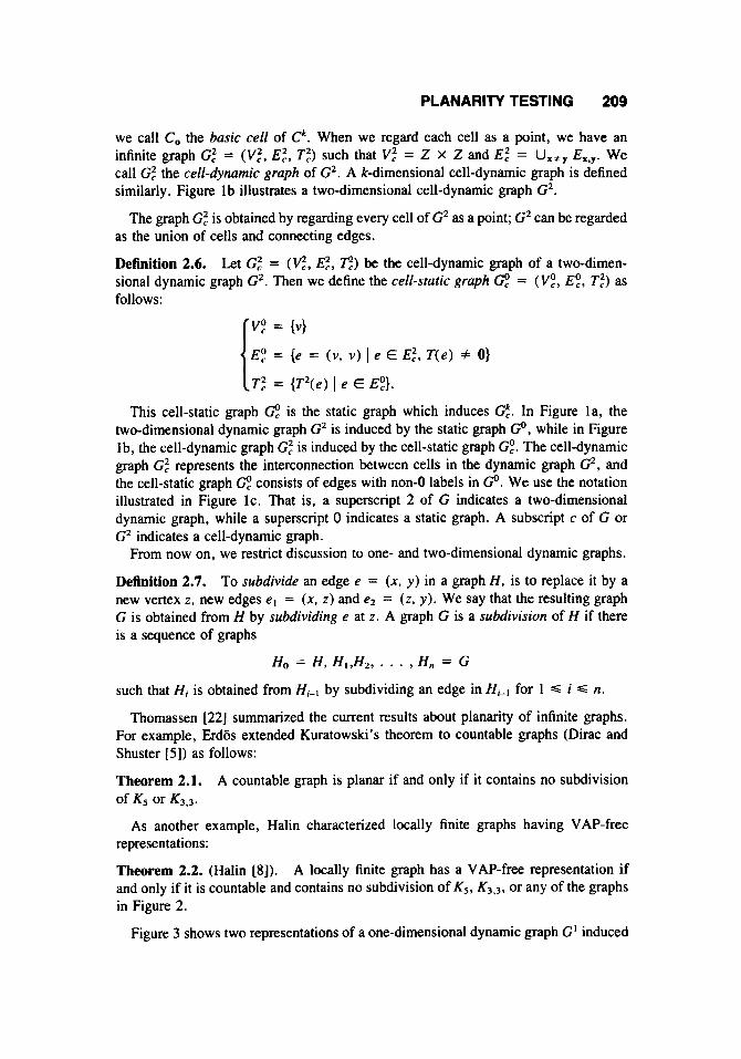
Theorem 2.2. (Halin [8]). A locally finite graph has a VAP-free representation if and only if it is countable and contains no subdivision of K5, K3.3, or any of the graphs in Figure 2.

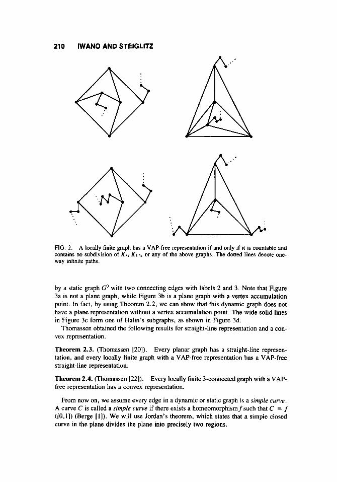
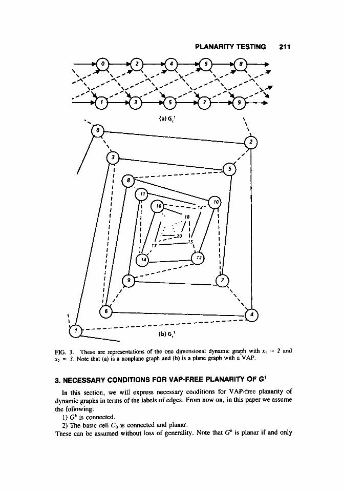
Figure 3 shows two representations of a one-dimensional dynamic graph GI induced


FIG. 2. A locally finite graph has a VAP-free representation if and only if it is countable and contains no subdivision of Ks. K3,,, or any of the above graphs. The dotted lines denote one- way infinite paths.

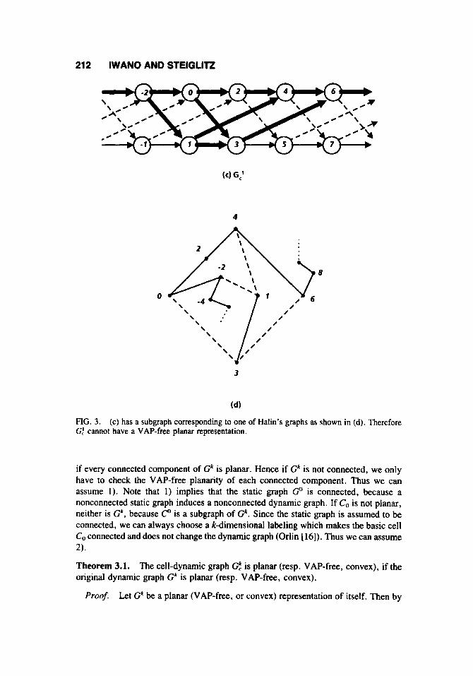
by a static graph GO with two connecting edges with labels 2 and 3. Note that Figure 3a is not a plane graph, while Figure 3b is a plane graph with a vertex accumulation point. In fact, by using Theorem 2.2, we can show that this dynamic graph does not have a plane representation without a vertex accumulation point. The wide solid lines in Figure 3c form one of Halin’s subgraphs, as shown in Figure 3d.

Thomassen obtained the following results for straight-line representation and a convex representation.

Theorem 2.3. (Thomassen [20]). Every planar graph has a straight-line representation, and every locally finite graph with a VAP-free representation has a VAP-free straight-line representation.

Theorem 2.4. (Thomassen [22]). free representation has a convex representation.

Every locally finite 3-connected graph with a VAP-

From now on, we assume every edge in a dynamic or static graph is a simple curve. A curve C is called a simple curve if there exists a homeomorphismfsuch that C = f ([O,l]) (Berge [ I ] ) . We will use Jordan’s theorem, which states that a simple closed curve in the plane divides the plane into precisely two regions.

PLANARITY TESTING 21 1

\ \

\ h

FIG. 3. x2 = 3. Note that (a) is a nonplane graph and (b) is a plane graph with a VAP.

These are representations of the one dimensional dynamic graph with x , = 2 and

3. NECESSARY CONDITIONS FOR VAP-FREE PLANARITY OF G' In this section, we will express necessary coriditions for VAP-free planarity of

dynamic graphs in terms of the labels of edges. From now on, in this paper we assume the following:

1) Gk is connected. 2) The basic cell C, is connected and planar.

These can be assumed without loss of generality. Note that Gk is planar if and only


\ \ \

/- /

\ \

3

FIG. 3. Cj cannot have a VAP-free planar representation.

(c) has a subgraph corresponding to one of Halin's graphs as shown in (d). Therefore

if every connected component of G' is planar. Hence if Gk is not connected, we only have to check the VAP-free planarity of each connected component. Thus we can assume 1). Note that 1) implies that the static graph Go is connected, because a nonconnected static graph induces a nonconnected dynamic graph. If Co is not planar, neither is Gk, because C" is a subgraph of G'. Since the static graph is assumed to be connected, we can always choose a k-dimensional labeling which makes the basic cell Co connected and does not change the dynamic graph (Orlin [ 161). Thus we can assume 2).

Theorem 3.1. The cell-dynamic graph G: is planar (resp. VAP-free, convex), if the original dynamic graph G' is planar (resp. VAP-free, convex).

Let G' be a planar (VAP-free, or convex) representation of itself. Then by Proof.


replacing each cell of G' by a point, we can get a planar (VAP-free, or convex) representation of Gt. 8

Thomassen showed the following about VAP-free, locally finite plane graphs.

Theorem 3.2. (Thomassen [22]). Let G be an infinite, locally finite, connected VAP- free plane graph. Then there exists an infinite straight line triangulation A of the plane such that G is isomorphic to a subgraph of A.

Note that dynamic graphs are locally finite by definition. Thus we can apply Theorem 3.2 to any connected VAP-free plane dynamic graph and show that its vertex set can be chosen to be integer lattice points of the plane as follows:

Corollary 3.1. Let G2 be a connected, VAP-free, plane graph. Then G2 is isomorphic to a subgraph of a plane graph r = (Tv, rE), where Tv C 2.

Let A be an infinite straight line triangulation of the plane such that G is isomorphic to a subgraph of A. Let p g l p 2 be a triangle of A. If necessary, we can expand the triangle p g l p 2 (with the rest of the graph) so that it contains at least three integer points. Let q,,q1q2 be a triangle such that qo, q l , and q2 are integer points in the triangle pg1p2. We can then replace the triangle p4p1p2 by the triangle q,,qlq2. By repeating this operation, we can obtain a triangulation of the plane A' whose vertices

Proof.

are integer points. Thus G is isomorphic to a subgraph of A'. 8

Let Gr = ( V j , E i , Tr) be the cell-dynamic graph of a one-dimensional dynamic = (e, e, Tr) be the cell-static graph where we will represent graph G' and let

the one-dimensional edge-labels by xi, suitably ordered as follows:

( V f = (4 Ef = {el, e2, . . . , em}, where

ei = ( v , v ) and T:(ei) = xi E Z such that

Since we are concerned with planarity, we can assume without loss of generality that xi > 0 for 1 d i d m, and that the edge-labels of @ are distinct, so that

(3.2) We have the following definition about 2-t4 paths induced by a p-edge (that is, an edge with label p).

Definition 3.1. Let each vertex of Vr be denoted by an integer. Suppose that there is a p-edge in Gr. Then each p-edge in Ct. induces a 2-@3 path PP.; = (Vp,i, Ep, i ) for 0 c i < p - 1 as follows:

0 < < x2 < * * - < x,.

Vp,i = {n 1 n = i (rnodp)}, I Ep.i = {(n, n + P) 1 n E Vp,i}* That is, Pp.i is a 2-w path consisting of p-edges and the nodes which are equal to i mod p. Note that Vr is the disjoint union of {V,.; 1 0 C i C p - I}.

From Theorem 3. I , VAP-free planarity of the cell-dynamic graph Gr is a necessary


m =2, x t = 1, x2 =2

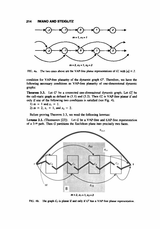
FIG. 4a. The two cases above are the VAP-free planar representations of G: with S 2.

condition for VAP-free planarity of the dynamic graph G'. Therefore, we have the following necessary conditions as VAP-free planarity of onedimensional dynamic graphs: Theorem 3.3. Let G' be a connected one-dimensional dynamic graph. Let Gy be the cell-static graph as defined in (3. I ) and (3.2). Then Gr is VAP-free planar if and only if one of the following two conditions is satisfied (see Fig. 4).

I ) m = 1 andx, = 1. 2 ) m = 2 , x l = I , and x2 = 2.

Before proving Theorem 3.3, we need the following lemmas:

Lemma 3.1. (Thomassen [22]). of a 2-00 path. Then G partitions the Euclidean plane into precisely two faces.

Let G be a VAP-free and EAP-free representation

t

m = 2, X I = 1, XI = 2

FIG. 4b. The graph Gf is p h a r if and only if G' has a VAP-free planar representation.


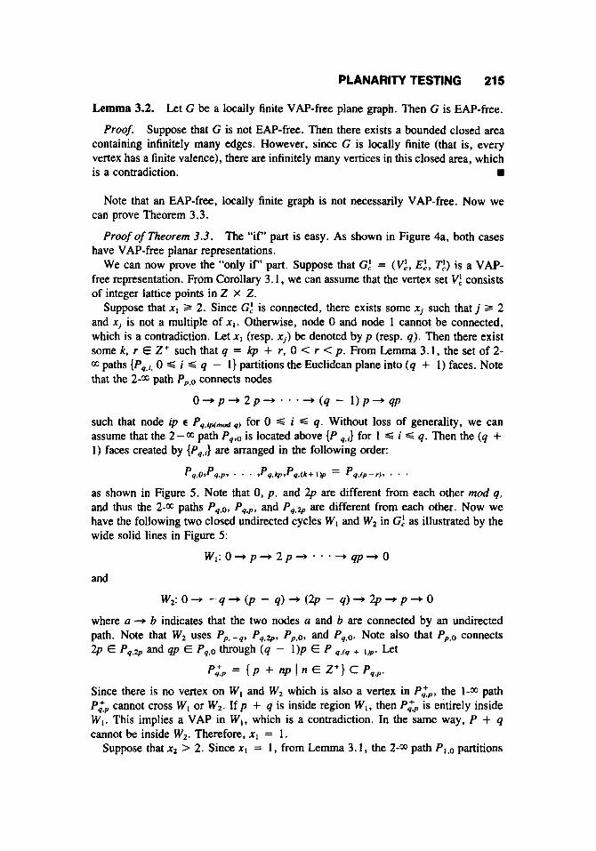
Lemma 3.2. Let G be a locally finite VAP-free plane graph. Then G is EAP-free.

Proof. Suppose that G is not EAP-free. Then there exists a bounded closed area containing infinitely many edges. However, since G is locally finite (that is, every vertex has a finite valence), there are infinitely many vertices in this closed area, which is a contradiction.

Note that an EAP-free, locally finite graph is not necessarily VAP-free. Now we can prove Theorem 3.3.

Proof of Theorem 3.3. The “if’ part is easy. As shown in Figure 4a, both cases have VAP-free planar representations.

We can now prove the “only i f ’ part. Suppose that Gr = (V!, E!, Tr) is a VAP- free representation. From Corollary 3.1, we can assume that the vertex set Vf consists of integer lattice points in 2 X Z.

Suppose that x , 2 2. Since G: is connected, there exists some xj such that j 3 2 and x j is not a multiple of xl. Otherwise, node 0 and node 1 cannot be connected, which is a contradiction. Let x1 (resp. x i ) be denoted by p (resp. q ) . Then there exist some k, r E Z+ such that q = kp + r , 0 < r < p . From Lemma 3.1, the set of 2- 03 paths { f q , i , 0 S i S q - 1) partitions the Euclidean plane into (q + 1) faces. Note that the 2-@3 path PpT0 connects nodes

o + p + 2 p - , * * *--, (q - 1 ) p - q p

such that node ip E P9,ip(mod9, for 0 S i 4 q. Without loss of generality, we can assume that the 2-03 path Pq,o is located above { P q,i} for 1 S i C q. Then the (q + 1) faces created by {P9,i} are arranged in the following order:

- pq,O,pq.p, . . . ,pq.hp,pq.U+l)p - p q . ( p - r I , * ,

as shown in Figure 5 . Note that 0, p , and 2p are different from each other mod q, and thus the 2-03 paths Pq.o, Pq,p, and Pq.@ are different from each other. Now we have the following two closed undirected cycles W 1 and W , in G! as illustrated by the wide solid lines in Figure 5:

w 1 : o - + p + 2 p - , * * * ~ q p - - , o

w2: 0- - q + ( p - q ) + (2p - q)-+ 2 p + p - , 0

and

where a + b indicates that the two nodes a and b are connected by an undirected path. Note that W , uses Pp.-9 , P , , , Ppa0, and Pq.o. Note also that Pp.o connects

P z p = { p + np 1 n E 2’) c Pq,p.

Since there is no vertex on W , and W, which is also a vertex in P:p, the 1-03 path P&, cannot cross W I or W 2 . If p + q is inside region W 1 , then P l P is entirely inside WI. This implies a VAP in W I , which is a contradiction. In the same way, P + q cannot be inside W,. Therefore, x1 = 1.

Suppose that x2 > 2 . Since x1 = 1, from Lemma 3.1, the 2-03 path P l s o partitions

2p E Pq,+ and 4p E Pq,o through ( q - 1)p E P q.fq + lip. Let


/"'

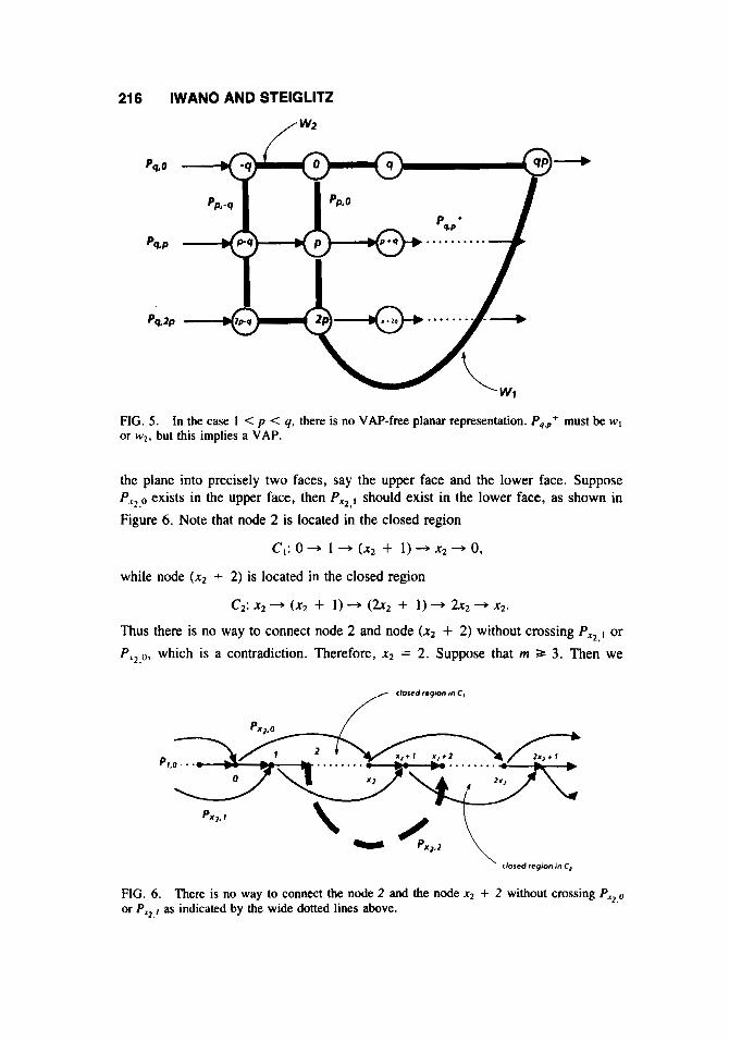
FIG. 5. or w2, but this implies a VAP.

In the case 1 < p < q. there is no VAP-free planar representation. P,+,+ must be w ,

the plane into precisely two faces, say the upper face and the lower face. Suppose qr2.,, exists in the upper face, then PX2, , should exist in the lower face, as shown in Figure 6. Note that node 2 is located in the closed region

c,: 0 + 1 3 (x2 + 1) --.* x2 3 0,

while node ( x 2 + 2) is located in the closed region

cz: x2 - (x2 + 1) 3 ( 2 x 2 + 1) + 2 x 2 3 xz.

Thus there is no way to connect node 2 and node (xz + 2) without crossing Px,,l or qr2,", which is a contradiction. Therefore, x2 = 2. Suppose that rn 3 3. Then we

closed region m C ,

. . . . . . . . ....... .

closed regron m C,

pxz.1

FIG. 6. There is no way to connect the node 2 and the node xz + 2 without crossing P,,,o or PX2,, as indicated by the wide dotted lines above.


have x I = 1, x2 = 2, and x3 > 2. An argument similar to that above also leads to a contradiction. Therefore, m S 2 and if m = 2, then xI = 1, x2 = 2. 8

4. VAP-FREE PLANARITY TESTING OF G' In this section we will show that VAP-free planarity testing of one-dimensional

dynamic graphs can be done in O(n) time, where n is the number of vertices in the basic cell. We use a finite graph G, instead of the infinite graph G' to test VAP-free planarity of GI. The graph G, associated with G' is defined as followed:

Definition 4.1. Let G' = (V ' , E' , T') be a one-dimensional dynamic graph. Let C, = (V,, be thwxth cell of G' for x E Z, where Ex., is the set of connecting edges between the xth and the yth cell as in Definition 2.5. Then we can define the finite graph G, = (V,, E,) as follows:

V, = Vo U Vl u V2 u V3 u {s, r } ,

E, = {Ex,, I 0 d x d y 6 3)

U { (s ,w) I 3 v s.r . ( v , w ) E x < 0 d y d 3)

U { ( v , t ) I 3 w s.t . ( v , w ) E E,,,, 0 G x G 3 < y } i u {(s, 0). Figure 4b shows an example of G,. Note that the vertex s (resp. t ) represents the cells of GI for i < 0 (resp. i > 3).

From Theorem 3.3, we can assume the following: 1) The cell graph of G' satisfied Ei.j = 9 for I i - j I 3 3 and EiVi+ # (4 for i E Z

(that is, there is a 1-edge and no p-edge for p > 2). 2) The basic cell is connected and planar. Then we have the following theorem:

Theorem 4.1. A one-dimensional dynamic graph GI, which satisfies the above as- sumptions, has a VAP-free planar representation if and only if the associated finite graph G, is planar.

Suppose that Gf is planar. Assume there is a 2-edge. (If not, the following proof can be easily modified.) Since there is at least a 1-edge and since the basic cell is connected, there is an undirected cycle

w: s + co + CI + c2 -+ c3 + t + s

in G,. Without loss of generality, we can assume that s, Co, CI, C2, C3, and t are located in this order from the left as shown in Figure 4b. Otherwise we can transform the graph to the desired form, without losing VAP-free planarity, by expanding the edge (s, r ) and rotating the graph along with the cycle W. From Jordan's theorem, the cycle W partitions the plane into exactly two regions. We call the inside (resp. outside) Ri, (resp. Rout). Note that the cycle W corresponds to the 2-m path in G. Note also that all edges in EovZ lie in either Ri, or R,, and the same is true for El .3 . If EOa2 lies in Ri, (resp. R,,,), E1.3 must lie in R,,, (resp. Ri,,). Let B be a closed region which contains only C, and C2, as shown by the shaded area in Figure 4b. Then we

Proof.


can obtain a VAP-free representation of C' by infinitely repeating B, because we can maintain the same sequence of 2-edges on the boundary of B.

Conversely, suppose that G' is VAP-free planar. We can assume that GI itself is a VAP-free plane graph. It is clear that the subgraph consisting of C-', Co, C,, C2, Cs, and C, is planar. Then Gf is obtained by contracting C-I (resp. C,) to the point s

Corollary 4.1. VAP-free planarity testing can be done in O(n) time for a one- dimensional dynamic graph GI, where n is the number of vertices in the basic cell of GI.

We can use any planarity testing algorithm which runs in time linear in the order of the vertex set (Hopcroft and Tajan [9], Lempel, Even, and Cederbaum 1151).

(resp. t ) and adding the edge (s, 1 ) .

Proof.

5. NECESSARY CONDITIONS FOR VAP-FREE PLANARITY OF G2

We also have similar necessary conditions for VAP-free planarity of two-dimensional dynamic graphs. Let GI! = (V:, E:, Tf) be the cell static graph with

v: = { v }

EY = {el, e2. . . . , em)

Tf(ei) = el = ( x i , yi) for 1 s i d rn. As in Section 3, we can assume that xi > 0 for 1 d i d rn and el # eJ for i # j . We can also assume that a dynamic graph G2 is connected and its basic cell Co is connected and planar. Let Gf = (Vf , Ef, Tf) be the cell graph of G2 with

V f = Z X Z

E: = U where x , y € z x z . x + y

= I e E E:, T f k ) = Y - x).

Theorem 5.1. The cell graph Gf is VAP-free planar if and only if one of the following two conditions is satisfied:

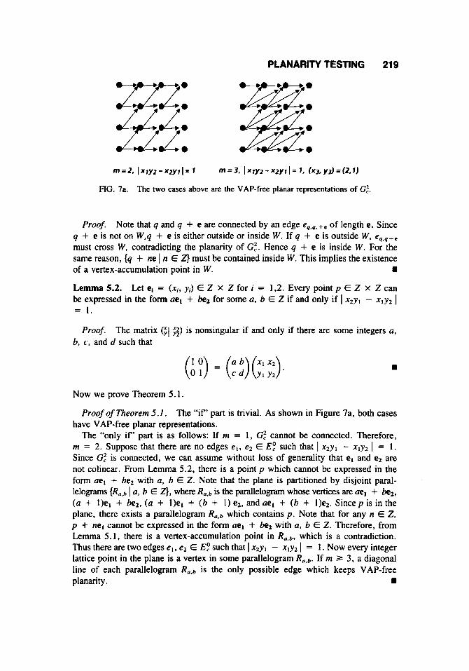
I ) rn = 2 and 1 xly2 - xgy, I = 1; that is, every point p E Z X Z can be expressed in the form ael + be2 for some a, b E Z.

2) rn = 3, I x l y 2 - x2yl 1 = 1 and e, = el - e2, e2 - el, or el + el; that is, e3 is a diagonal line of the parallelogram (0, el, e2, el + e2).

Before proving Theorem 5.1, we need the following lemma:

Lemma 5.1. Let W be a cycle in Gf such that

W : p o - + p , + ' * - + p m - , p o

for p i E <. Suppose there exists a point q E V," inside W and some e E such that q + ne f pi for any pi on W and for any n E Z. Then if Gf is planar, there exists a vertex-accumulation point inside W.


Proof. Note that q and q + e are connected by an edge eq,4. + e of length e. Since q + e is not on W,q + e is either outside or inside W. If q + e is outside W, eq,q+e must cross W, contradicting the planarity of Gf. Hence q + e is inside W. For the same reason, {q + ne 1 n E Z} must be contained inside W. This implies the existence

W

Lemma 5.2. Let el = (x i , yi) E Z X Z for i = 1,2. Every point p E Z x 2 can be expressed in the form ael + bez for some a, b E 2 if and only if I xzy l - xlyz I = 1.

of a vertex-accumulation point in W.

Proof. The matrix ($; $$) is nonsingular if and only if there are some integers a, b, c, and d such that

W

Now we prove Theorem 5.1.

Proof ofTheorern 5.1. The “if‘ part is trivial. As shown in Figure 7a, both cases have VAP-free planar representations.

The “only if’ part is as follows: If m = 1, G: cannot be connected. Therefore, rn = 2. Suppose that there are no edges e l , e2 E E: such that I x z y l - x l y z I = 1. Since Gf is connected, we can assume without loss of generality that el and ez are not colinear. From Lemma 5.2, there is a point p which cannot be expressed in the form ael + bez with a, b E Z. Note that the plane is partitioned by disjoint paral- lelograms {Ro,b I a, b E Z}, where Ra,b is the parallelogram whose vertices are ael + bez, ( a + I)el + bez, ( a + l)el + (b + 1) ez, and ae, + ( b + l)ez. Sincep is in the plane, there exists a parallelogram Rae6 which contains p. Note that for any n E Z, p + nel cannot be expressed in the form ael + bez with a, b E Z. Therefore, from Lemma 5.1, there is a vertex-accumulation point in Ra,b, which is a contradiction. Thus there are two edges el, e2 E E? such that I xzyl - xly2 I = 1. Now every integer lattice point in the plane is a vertex in some parallelogram Ra.b. If rn 3 3, a diagonal line of each parallelogram Ro,b is the only possible edge which keeps VAP-free planarity. W


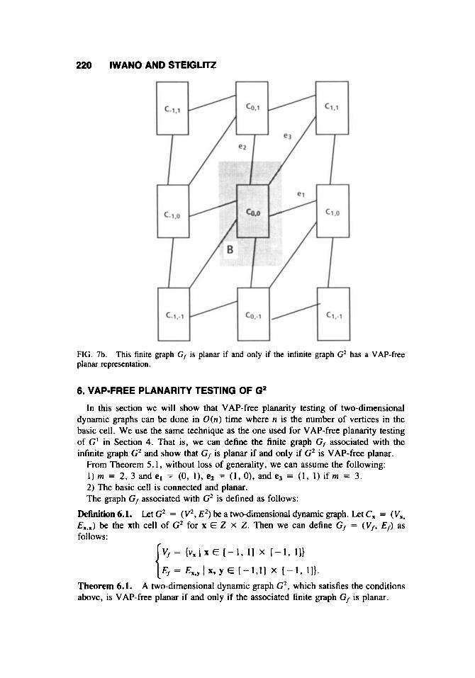
FIG. 7b. planar representation.

This finite graph Gf is planar if and only if the infinite graph G2 has a VAP-free

6. VAP-FREE PLANARITY TESTING OF G2 In this section we will show that VAP-free planarity testing of two-dimensional

dynamic graphs can be done in O(n) time where n is the number of vertices in the basic cell. We use the same technique as the one used for VAP-free planarity testing of G' in Section 4. That is, we can define the finite graph G, associated with the infinite graph G2 and show that G, is planar if and only if G2 is VAP-free planar.

From Theorem 5 . I , without loss of generality, we can assume the following: 1 ) m = 2, 3 and el = (0, I ) , e2 = (1, 0). and e3 = (1 , 1) if rn = 3. 2) The basic cell is connected and planar. The graph G, associated with G2 is defined as follows:

Definition 6.1. Let G2 = ( V2, E2) be a two-dimensional dynamic graph. Let C, = ( Vx, be the xth cell of G2 for x E 2 x Z. Then we can define G, = (Vf, E,) as

follows:

V , = { v x ( x E [ - l , I l x [ - 1 , 1 ] }

E, = E x , Y I X, y E [ - 1 , 1 1 X I - 1 , 11). i Theorem 6.1. above, is VAP-free planar if and only if the associated finite graph Gf is planar.

A two-dimensional dynamic graph G2, which satisfies the conditions


Proof. Suppose that GZ is planar. Since G, is a finite subgraph of G2, G, is also planar.

Conversely, suppose that G, is planar. Since every cell is connected, there is a cycle W connecting C- - C1. - I , C l , I , and C- I , I . We can assume that Co,o is located inside the cycle W. Let B be a rectangle which contains only Co,o as shown in Figure 7b. Then a VAP-free representation of GZ is obtained by repeating B at each cell.

Corollary 6.1. VAP-free planarity testing can be done in O(n) time for the connected two-dimensional dynamic graph G2 where n is the number of vertices in the basic cell of GZ.

The planarity testing can be done in O(l V, I ) time (Hopcroft and Tarjan Proof, [9], Lempel, Even, and Cederbaum [15] and 1 V, 1 = O(n). rn

7. CONCLUSIONS

We investigated VAP-free planarity testing of one- and two-dimensional dynamic graphs. First, we showed necessary conditions for VAP-free planarity of dynamic graphs in terms of the edge labels. Then we showed that there is a finite graph which is no larger than a constant multiple times the size of the basic cell and is planar if and only if the original dynamic graph is VAP-free planar. Therefore, VAP-free planarity testing of dynamic graphs can be done in O ( n ) time where n is the number of vertices in the basic cell.

Generally speaking, the regularity of dynamic graphs makes problems like planarity- testing easier, because we can transform them to problems of static graphs or sufficiently small finite graphs. Using this idea, the authors are now investigating other problems for two-dimensional dynamic graphs, such as weak connectivity, Eulerian paths, 2- colorability, and the longest path problem (Iwano [13]).

ACKNOWLEDGMENT The authors wish to thank the anonymous referees for their thoughtful and useful comments.

References [ I ] C. Berge, Topological Spaces (translated by E. M. Patterson), The Macmillan Company,

New York, 1963. [2] P. R. Cappello and K. Steiglitz, Digital signal processing applications of systolic algo-

rithms. CMU Conference on VLSI Systems and Computations, H. T. Kung, Bob Sproull, and Guy Steele (eds.), Computer Science Press, Rockville, MD. 1981.

[3] N. Christofides, Graph Theory: An Algorithmic Approach, Academic Press, London, 1975. [4] G. B. Dantzig, W. 0. Blattner, and M. R . Rao, Finding a cycle in a graph with minimum

cost to time ratio with application to a ship routing problem. in Int. Symp. on Theory of Graphs, P. Rosentiehl (ed.), Dunad, Paris; Gordon and Breach, New York. 1967, pp. 77-83.

[5 ] G. A. Dirac and S. Schuster, A theorem of Kuratowski. Indag. Math. 16 (1954), 343- 348.

[6] B. Griinbaum and G. C. Shephard, lsohedral tilings of the plane by polygons. Comment. Math. Helv. 53 (1978), 542-571.


[7] B. Griinbaum and G. C. Shephard, The geometry of planar graphs. Combinatorics Y . Temperley (ed.), London Math. Soc. Lecture Notes 52, Cambridge Univ. Press, London. 1981. pp. 124-150.

[8] R. Halin, Zur haufungspunktfreien Darstellung abziihlbarer Graphen in der Ebene. Arch. Math. (Basel) 17 (1966), 239-243.

[S] J . Hopcroft and R. E. Tarjan, Efficient planarity testing. JACM 21 (1971), 549-568. [ 101 K. Iwano and K. Steiglitz. A semiring on convex polygons and zero-sum cycle problems.

Tech. Rep. CS-TR-053-86, Computer Science Dept., Princeton Univ., Princeton, N.J., Sept. 1986.

[ 1 I ] K. Iwano and K. Steiglitz, 1986b. Optimization of one-bit full adders embedded in regular structures. IEEE Trans. Acoustics, Speech, and Signal Proc. ASSP-34 (1986). 1289- 1300.

[I21 K . lwano and K. Steiglitz, 1987a. Testing for cycles in infinite graphs with periodic structure. Proc. 19th Annual ACM Symposium on Theory of Computing. May 1987, 46- 55.

1131 K. Iwano, Two-dimensional dynamic graphs and their VLSI applications. Ph. D . disser- tation, Department of Computer Science, Princeton University. Oct., 1987.

114) E. L. Lawler, Optimal cycles in doubly weighted directed linear graphs. in Int. Symp. on Theory ofGraphs, see P. Rosentiehl (ed.), Paris, Dunad; New York, Go:.don and Breach,

[ 151 A. Lempel, S. Even, and I. Cederbaum, An algorithm for planarity testing of graphs. in Int. Symp. on Theory of Graphs, P. Rosentiehl (ed.), Dunod, Paris; New York, Gordon and Breach, 1967, pp. 215-232.

1161 J. Orlin, Some problems on dynamic/periodic graphs. in Progress in Combinarorial Op- timization, W. R. Pulleybank (ed.), Academic, Orlando, 1984, pp. 273-293.

1171 W. R. Pulleybank (ed.), Progress in Combinarorial Optimization, Academic Press, Or- lando, 1984.

118) R. Reiter. Scheduling parallel computation. J. ACM 15 (1968), 590-599. [I91 P. Rosentiehl (ed.), fnt. Symp. on Theory OfGraphs, Dunod. Paris, Gordon and Breach,

[20J C. Thomassen, Straight line representations of infinite planar graphs. J . London Math.

121 ] C. Thomassen, Planarity and duality of finite and infinite graphs. J . Combinatorial Theory

1221 C. Thomassen, Infinite graphs. in Selected Topics in Graph Theory 2 edited L. W. Beineke

1967, pp. 209-213.

New York, 1967.

SOC. (2) 16, (1977), 41 1423.

( B ) 29 (1980). 244-271.

and R. J. Wilson (eds.), Academic Press, New York, 1983.

Received January, 1987. Accepted August, 1987.

Documents

Planarity testing of doubly periodic infinite graphs