Picture Maze Generation by Successive Insertion of Path ... structure is kept maintained even if the maze ... However, in Fig. 1, vertices are placed on (odd, odd ... Fig. 4 (b) and

British Journal of Mathematics & Computer Science 4(24): 3444-3463, 2014

ISSN: 2231-0851

SCIENCEDOMAIN international www.sciencedomain.org

______________________________________________________________________________________________________________________

_____________________________________

*Corresponding author: [email protected];

Picture Maze Generation by Successive Insertion of Path

Segment

Tomio Kurokawa

1*

1Department of Information Science, Aichi Institute of Technology, Toyota 470-0392, Japan.

Article Information

DOI: 10.9734/BJMCS/2014/12048

Editor(s):

(1) Linning Ye, School of Economic Information Engineering, Southwestern University of Finance and Economics,

China.

Reviewers:

(1) Tzvetalin S. Vassilev, Department of Computer Science and Mathematics, Nipissing University, Canada.

(2) Anonymous, Georgia Southern University, Statesboro, USA.

(3) Anonymous, India.

Complete Peer review History: http://www.sciencedomain.org/review-history.php?iid=699&id=6&aid=6362

Received: 15 June 2014

Accepted: 01 September 2014

Published: 06 October 2014

_______________________________________________________________________

Abstract

Picture maze is a maze on which some picture appears when it is solved. This paper aims to

present a very simple method to construct a picture maze. It is always possible to construct a

spanning tree on a connected region of a binary picture. A spanning tree connects all vertices on

the region. A 2-by-2 extended picture of a connected picture is the one such that each cell in the

picture is transformed to four cells which constitute a square block with the cells. Then by

analogy, it is always possible to construct a block spanning tree on the extended picture region,

where a block is the square unit of four cells. Construction of the block spanning tree and the

generation of the corresponding Hamiltonian path can be done at the same time. The

Hamiltonian path is constructed along a data structure of a linked list in a simple manner. It

traverses every cell on the 2-by-2 extended picture. The similar procedure but with the smaller

block with two vertices, instead of four, can be applied to a non-extended picture, an ordinary

one, which produces a near Hamiltonian path, which can then be a maze solution path. The near

Hamiltonian path traverses nearly all the vertices on the picture, hence depicting a picture on the

maze when it is solved. This paper demonstrates the method and its efficiency.

Keywords: Maze, Picture maze, Spanning tree, Block spanning tree, Path extension, Hamiltonian

path

Original Research Article

British Journal of Mathematics & Computer Science 4(24), 3444-3463, 2014

3445

1 Introduction

Maze generation by computing with square grids has been around for some years. The article [1]

showed various algorithms to generate a square grid based maze, usually used, relating with graph

theory. Hosokawa [2] presented a number of maze generation algorithms with the relation

between path, wall, and coordinates. Xu and Kaplan [3] illustrated complex mazes emphasizing

aesthetics for the maze. They also introduced a picture maze [4] called 'Maze-a-pix' by illustrating

a sample picture maze, which is provided by Conceptis, Ltd. [5]. However, the method of the

picture maze generation was not given. The internet site of the company shows various picture

mazes and states a history of computer generated picture maze. Okamoto and Uehara [6]

demonstrated an automatic generation algorithm for a picture maze by constructing a Hamiltonian

path which fills up the picture region. However, the path is generated on the 2-by-2 extended

picture array. The maze is so constructed in the research that the player obtains the solution path

by filling up all the path cells on the maze and by painting the picture region. Hamada [7] and [8]

improved the method [6] by enabling to place the start and goal at different positions. Ikeda and

Hashimoto [9] illustrated a picture maze generation method by using simulated annealing.

Kurokawa, Mori, and Mizuno [10]-[12] took a different approach and demonstrated a method to

generate a picture maze by making use of the picture contours. In this method, all the contours are

extracted and are incorporated into the picture maze. It is a very flexible method and can be

applicable to a wide range of binary pictures. F.J. Wong and S. Takahashi [13] constructed a

hybrid picture maze from two photograph images. This maze is not based on square grids like the

mazes but on the special grids computed from the image. Two photo pictures are overlapped in the

maze. The maze player depicts an outline of one picture on the other picture background.

2 Maze Structure

There are a number of different representation structures of a square grid maze. This paper uses

one of them and it is explained in this section. A computer constructed maze is usually represented

by a two-dimensional array. Such a maze consists of path and wall. A path cell is either a vertex or

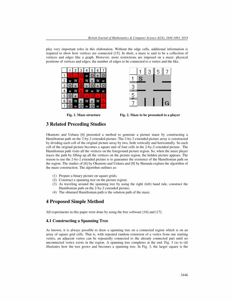
an edge (of a graph). Fig. 1 is a sample maze array of size 7x7---where '◎' is a vertex; 'e' is an

edge, and 'W' and 'w' are walls. A vertex is placed one in every two cells horizontally and

vertically. An edge represents the connection between the two vertices. Diagonally adjacent cells

to a vertex are wall cells; there are four such cells around a vertex; the vertically or horizontally

adjacent cells to a vertex are edge or wall cells. If the cell represents the connection between the

two vertices, then it is an edge cell; otherwise it is a wall cell.

The connection between the two vertices is 4-way, vertical or horizontal; and no diagonal

connection is allowed. The entire path routes in a maze organize a spanning tree. A vertex and an

edge alternately appear along a path. The maze solution of Fig. 1 is the path from the start (S) to

the goal (G), which is one of the paths from a vertex (the tree root) to another vertex (a leaf). The

maze structure is kept maintained even if the maze is shifted in any direction one or more

positions on the array. However, in Fig. 1, vertices are placed on (odd, odd) coordinates.

If the walls are thinned [14], the maze becomes as presented in Fig. 2. This maze, to be presented

to a player, actually consists of two kinds of cells: path and wall. However, it represents the

corresponding graph with vertices and edges, which cannot be otherwise represented as simply as

this structure. So the maze of this structure is said to be an elaborately organized graph. The edges


3446

play very important roles in this elaboration. Without the edge cells, additional information is

required to show how vertices are connected [15]. In short, a maze is said to be a collection of

vertices and edges like a graph. However, more restrictions are imposed on a maze: physical

positions of vertices and edges; the number of edges to be connected to a vertex and the like.

Fig. 1. Maze structure

Fig. 2. Maze to be presented to a player

3 Related Preceding Studies

Okamoto and Uehara [6] presented a method to generate a picture maze by constructing a

Hamiltonian path on the 2-by-2 extended picture. The 2-by-2 extended picture array is constructed

by dividing each cell of the original picture array by two, both vertically and horizontally. So each

cell of the original picture becomes a square unit of four cells in the 2-by-2 extended picture. The

Hamiltonian path visits all the vertices on the foreground picture region. So, when the maze player

traces the path by filling up all the vertices on the picture region, the hidden picture appears. The

reason to use the 2-by-2 extended picture is to guarantee the existence of the Hamiltonian path on

the region. The studies of [6] by Okamoto and Uehara and [8] by Hamada explain the algorithm of

the maze construction. The algorithm outlines as:

(1) Prepare a binary picture on square grids;

(2) Construct a spanning tree on the picture region;

(3) As traveling around the spanning tree by using the right (left) hand rule, construct the

Hamiltonian path on the 2-by-2 extended picture;

(4) The obtained Hamiltonian path is the solution path of the maze.

4 Proposed Simple Method

All experiments in this paper were done by using the free software [16] and [17].

4.1 Constructing a Spanning Tree

As known, it is always possible to draw a spanning tree on a connected region which is on an

array of square grid cells. That is, with repeated random extension of a vertex from one starting

vertex, an adjacent vertex can be repeatedly connected to the already connected part until no

unconnected vertex exists in the region. A spanning tree completes at the end. Fig. 3 (a) to (d)

illustrates how the tree grows and becomes a spanning tree. In Fig. 3, the larger square is the

1 2 3 4 5 6 7

1 S e ◎ w ◎ e ◎

2 w W e W e W w

3 ◎ e ◎ e ◎ e ◎

4 w W e W w W w

5 ◎ e ◎ e ◎ e ◎

6 e W e W e W e

7 ◎ w ◎ w ◎ w G


3447

picture region, where the tree can grow. The red cell with a green dot is the vertex and the darker

gray cell is an edge. Staring with the red cell with a black dot, the tree grows as the random

connection of an adjacent vertex to the tree proceeds. The connection is made with the edge (dark

gray cell). Fig. 3 (d) is the final spanning tree.

4.2 Construction of Block Spanning Tree and the Hamiltonian Path This subsection describes how to construct a Hamiltonian path which fills up all the vertices on

the 2-by-2 extended picture simultaneously building the block spanning tree. It is by the analogy

of the method of the spanning tree construction in the previous subsection 4.1.

Each cell in the original picture corresponds to the block of four cells in the 2-by-2 extended

picture. This provides the principle that if a vertex extension on the original picture to construct a

tree is possible, then the corresponding extension of the block of four vertices on the extended

picture is possible. If the extension is repeated until all blocks are connected, a spanning tree with

blocks is to be completed on the picture region at the end. This means that it is always possible to

construct such a spanning tree on the extended picture. The block trees so generated are shown in

Fig. 4 (a)-(d), where they are with the simultaneously being generated path which traverses all the

vertices of the block trees without repetition of any vertices or edges. Fig. 4 (d) illustrates the

block spanning tree as well as the final Hamiltonian path on the picture region.

Fig. 4 (a) shows the starting block. The extension could be made to three directions: to the right, to

the top or to the left. The extension to the bottom is not allowed because it is out of the picture

region. Fig. 4 (b) illustrates the second extension made to the left as a random process. The path

starts at the vertex with green color, going through the alternating sequence of edge (gray) and

vertex (red) and ends at the vertex of blue color. Fig. 4 (b) and (c) are the intermediate results.

Fig. 4 (d) is the final block spanning tree and the constructed Hamiltonian path.

Whenever one square unit of four vertices is added to the tree, four vertices and five edges are

connected in the proper order and one edge at the extending position is deleted so as to make the

path go through all the vertices which constitute the tree being constructed. When the tree finally

becomes a block spanning tree, the path becomes the Hamiltonian path for the final block tree,

which fills up all the vertices on the extended picture region. If the final block tree is a block

spanning tree, the final path is the Hamiltonian path.

To construct the Hamiltonian path and the block spanning tree at once, a data structure of linked

list is useful and efficient to hold the positions of vertices and edges for the path being organized.

The list, which is the linked nodes of x, y coordinates of cell position and vertex number, holds the

sequence of vertices and edges in the order for which the vertices and edges appear on the path.

Use of the list provides an efficient way to find the path place where the next block path segment

is to be connected as well as to insert a path segment into the path. It makes it needless to traverse

the tree while constructing the Hamiltonian path. By this method, the block spanning tree and

the Hamiltonian path are constructed at once. An experimentally organized list is illustrated in

section 6.

British Journal of M

(a)

Fig. 3. How a tree grows and becomes a spanning tree

(a)

Fig. 4. Construction of block spanning tree with t

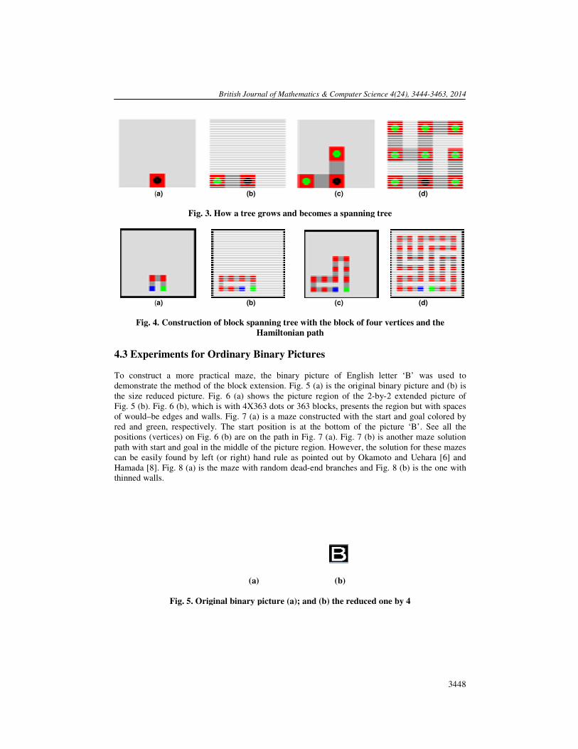
4.3 Experiments for Ordinary Binary Pictures To construct a more practical maze, the binary picture of English letter ‘B’ was used to

demonstrate the method of the block extension. Fig

the size reduced picture. Fig. 6

Fig. 5 (b). Fig. 6 (b), which is with 4X363 dots or 363 blocks,

of would–be edges and walls. Fig

red and green, respectively. The start position is at the bottom of the picture ‘B’. See all the

positions (vertices) on Fig. 6 (b) are on the path in Fig

path with start and goal in the middle of the picture region. However, the solution for the

can be easily found by left (or right)

Hamada [8]. Fig. 8 (a) is the maze with random

thinned walls.

Fig. 5. Original binary picture (a)

British Journal of Mathematics & Computer Science 4(24), 3444-3

(b) (c) (d)

How a tree grows and becomes a spanning tree

(b) (c) (d)

Construction of block spanning tree with the block of four vertices and the

Hamiltonian path

4.3 Experiments for Ordinary Binary Pictures

To construct a more practical maze, the binary picture of English letter ‘B’ was used to

demonstrate the method of the block extension. Fig. 5 (a) is the original binary picture and (b) is

. 6 (a) shows the picture region of the 2-by-2 extended picture of

which is with 4X363 dots or 363 blocks, presents the region but with spaces

ls. Fig. 7 (a) is a maze constructed with the start and goal colored by

. The start position is at the bottom of the picture ‘B’. See all the

(b) are on the path in Fig. 7 (a). Fig. 7 (b) is another maze solution

path with start and goal in the middle of the picture region. However, the solution for the

left (or right) hand rule as pointed out by Okamoto and Uehara [6] and

(a) is the maze with random dead-end branches and Fig. 8 (b) is the one with

(a) (b)

Original binary picture (a); and (b) the reduced one by 4

3463, 2014

3448

he block of four vertices and the

To construct a more practical maze, the binary picture of English letter ‘B’ was used to

inal binary picture and (b) is

2 extended picture of

presents the region but with spaces

start and goal colored by

. The start position is at the bottom of the picture ‘B’. See all the

maze solution

path with start and goal in the middle of the picture region. However, the solution for these mazes

as pointed out by Okamoto and Uehara [6] and

the one with


(a)

Fig. 6. (a) 2-by-2 extended picture

(a)

Fig. 7. (a) Block Hamiltonian path with

Hamiltonian path with

(a)

Fig. 8. (a) Maze with random dead


(a) (b)

extended picture; and (b) the one with would-be edges inserted

(a) (b)

(a) Block Hamiltonian path with the start and goal at the bottom; and (b) block

amiltonian path with the start and goal in the middle of the picture.

(b)

Maze with random dead-end branches; and (b) the same maze with thinned walls

3463, 2014

3449

be edges inserted

(b) block

ame maze with thinned walls


5 A Method with Smaller Block

5.1 Constructing a Near H Another block extension method was tried to demonstrate the picture maze generation using an

ordinary binary picture instead of the 2

includes only two vertices instead of four, was used

starts with the two vertices (green

upward as shown by Fig. 9 (b). Two vertices and three edges are also inserted into the

proper order as done in the block method with four vertices of the previous section. The spanning

tree completes as in Fig. 9 (d). This method is supposed to be more flexible because the block is

smaller. Similar extensions or methods

by Wong and Takahashi, but in different situations.

(a)

Fig. 9. Construction of block spanning tree with the block of two vertices and the

5.2 Practical Application A practical but simple picture of letters ‘AB’ was tried for a demonstration.

of ‘AB’ which was reduced by 6 from an original picture. The maze was to be constructed from

this reduced picture by employing the method of subsection 5.1. In this case, the picture

extended. Fig. 11 illustrates the initial path which is just a

entrance vertex (a green point at the extreme

point at the extreme left) passing through bo

two regions in which the path grows

contours of ‘AB’ in Fig. 11 are just to show where the initial path line goes through. The contours

are not directly related with the path construction. Fig. 12 shows an early stage of the path

extension. The extension occurs in both regions of ‘A’ and ‘B’; where a Hamiltonian path is tried

to be generated. This means that the entire path from the entrance to t

once. More importantly, those initial extensions are made in both directions upward and

downward in many positions. Therefore the maze cannot be solved easily with only one of the left

or right hand rules. The path is constructed

Fig. 13 is a completed maze solution path. A number of black dots are seen. These are the vertices

not on the maze solution path. The path failed to become a Hamiltonian path. Therefore, it should

be called as a near Hamiltonian path. The complete avoidance of the black points is usually

impossible. This is probably why the 2

the picture ‘AB’ appears clearly in Fig.


with Smaller Block

Hamiltonian Path

Another block extension method was tried to demonstrate the picture maze generation using an

ordinary binary picture instead of the 2-by-2 extended one. In this case, the smaller block

includes only two vertices instead of four, was used to extend the path. As Fig. 9 (a) illustrates, it

two vertices (green and blue) and the edge between the two. The first extension is

upward as shown by Fig. 9 (b). Two vertices and three edges are also inserted into the

er as done in the block method with four vertices of the previous section. The spanning


extensions or methods appear in the studies [9] by Ikeda and Hashimoto and [13]

by Wong and Takahashi, but in different situations.

(b) (c) (d)

Construction of block spanning tree with the block of two vertices and the

Hamiltonian path

re of letters ‘AB’ was tried for a demonstration. Fig. 10 is the picture


this reduced picture by employing the method of subsection 5.1. In this case, the picture

illustrates the initial path which is just a straight path, the simplest, from the

at the extreme right) to a boundary position of the exit vertex (a red

point at the extreme left) passing through both of the foreground picture parts of ‘AB’.

two regions in which the path grows---‘A’ and ‘B’. Those are the foreground parts of ‘AB’. The


directly related with the path construction. Fig. 12 shows an early stage of the path


to be generated. This means that the entire path from the entrance to the exit was constructed at



or right hand rules. The path is constructed with the mixed rules. The details are given in section 6.




impossible. This is probably why the 2-by-2 extended picture was used in the study [6]. However,

the picture ‘AB’ appears clearly in Fig. 13.

3463, 2014

3450

Another block extension method was tried to demonstrate the picture maze generation using an

block, which

As Fig. 9 (a) illustrates, it

) and the edge between the two. The first extension is

list in the

er as done in the block method with four vertices of the previous section. The spanning


eda and Hashimoto and [13]

Construction of block spanning tree with the block of two vertices and the

Fig. 10 is the picture


this reduced picture by employing the method of subsection 5.1. In this case, the picture was not

, the simplest, from the

right) to a boundary position of the exit vertex (a red

There are

‘A’ and ‘B’. Those are the foreground parts of ‘AB’. The


directly related with the path construction. Fig. 12 shows an early stage of the path


he exit was constructed at



with the mixed rules. The details are given in section 6.




2 extended picture was used in the study [6]. However,


3451

Since the straight path lines are often easily seen before the solution is obtained [12], some

zigzags were added to hide them, using the same path extension method, as shown in Fig. 14. By

the way, horizontal and vertical straight lines or slopes with near 45 degree are often easily seen

before the maze is solved. After dead end branches were added and walls were thinned, the final

maze was finished as in Fig. 15. Fig. 16 is the maze with the solution path.

By the way, some more general procedures were suggested in the studies [9] and [13] for the

initial path generation.

Fig. 10. Picture of ‘AB’ already reduced by 6 Fig. 11. Initial straight solution path for ‘AB’

Fig. 12. Early stage of solution path

construction for ‘AB’

Fig. 13. Final solution path for ‘AB’

Fig. 14. Final solution path with zigzag for ‘AB’


Fig. 16.


Fig. 15. Final maze for ‘AB’

Fig. 16. Picture maze of ‘AB’ solved

3463, 2014

3452


3453

6 Discussion In this subsection, more details are given about the construction of the block spanning tree and the

corresponding Hamiltonian path.

6.1 Outline of the Algorithm for the Hamiltonian Path Construction Figs. 17 to 19 illustrate how the tree and the path are developed on the same picture region as

Fig. 4, that is, the 2-by-2 extended picture region with 9 blocks. The path construction algorithm is

given as:

1) Construct the path of the initial block in the array and the list (Fig. 17 (a) and (b));

2) Find a proper position on the path to which a new block is connected;

3) Delete one edge between the two adjacent vertices (at the above proper position) to

which next block path segment is inserted. Put the four vertices and the five edges in the

appropriate order on the array and insert them into the list at the position so that the

vertices and edges together organize one path;

4) Repeat 2) to 3) until all blocks are connected.

Fig. 17 to Fig. 19 illustrates only the model case. However, the above algorithm is applicable to

more practical pictures, which will be later explained. Fig. 17 (a) is the initial path with the

numbered vertices. The number, though not required for the path construction, explains the order

in which the vertices are inserted into the list. Fig. 17 (b) shows the list on which the number and x

and y coordinate addresses on the maze array and along the path are written. This illustrates that

the path starts with the vertex of ‘1’ and visiting the vertices in the order ‘2’, ‘3’, and ‘4’ which is

the goal. x and y addresses of vertices ‘1’ to ‘4’ agree between Fig. 17 (a) and (b). Fig. 18 (a) and

(b) show the situation where the second block is connected. The vertex sequence in the list is in

Fig. 18 (b) which also well corresponds with Fig. 18 (a). What was actually done is as follows:

Given the situation of Fig. 17, the edge between vertices ‘1’ and ‘2’ was first removed and then an

edge and a vertex were inserted alternately with the vertex order of ‘5’, ‘6’, ‘7’ and ‘8’. The

selection of the list position where to insert the block path segment is the random process. Fig. 19

is the final Hamiltonian path; the numbers attached to vertices show the order in which they are

inserted into the list. The visiting order of the vertex on the path is illustrated on the path itself.

The order is based on the left (or right) hand rule.

(a) (b)

Fig. 17. Initial block of four vertices


3454

(a) (b)

Fig. 18. Second stage of path construction

Fig. 19. Final Hamiltonian path: vertex 30 is at (3,3) and vertex 6 is at (13,13)

6.2 C Program Code, Explanation, Algorithm, Theorem and Proof

The essential part of the C program code, which actually produced Fig. 17 to Fig. 19 and Fig. 7

(with a little change), is given in Fig. 20. This code follows the algorithm given in subsection 6.1.

6.2.1 C program code explanation

Line 2 defines the pointers. p and k_pointer are the pointers which point to the nodes in the linked

list. The node has the fields of the maze array coordinates of x, y, the vertex number n and the link

next. The array t defined on lines 4 to 8 is to provide offsets for determining x and y position of

edges and vertices which are to be inserted into the path. This table array consists of four parts as

in Fig. 21, which will be explained later. The path eventually grows to a Hamiltonian path. Line 9

defines table c for the offset values to compute the center position of the initial block from which

a Hamiltonian path grows. This table is used on line 28. The function on line 10 does two jobs:

first is to make srcze array, the dotted picture like Fig. 6 (b), with 0 for the foreground picture

cells and 1 for the background; second is to initialize dze array with all 1, on which the

Hamiltonian path is to be constructed with 0 on the path cells. Line 11 gives the start x1 and y1

position and the block extension direction m = 0 (up) and h=m (initial block direction). To make


3455

the correspondence with the Fig. 17 to Fig. 19, m = 0 (h=0), x1=9, and y1=15 were specified. For

these values, the center of the block is (8, 12), and the start vertex (vn=1) is at (9, 13).

Other m, x1 and y1 can be specified. If m=2 (h=2), x1=7, and y1=7, the Hamiltonian path

eventually became as in Fig. 22. By the way, for this model case of 9 blocks, the maze picture

array srcze is 0 at all odd positions (odd, odd) within the square from (3, 3) to (13, 13), and 1 at

other positions.

Line 12 sets p to head (head pointer of the list) and the first vertex number vn to 1. Lines 13 to 17

draw the first block path on dze and insert the path into the list. The function insert_after has the

following C prototype:

��_��(�� , �� , �� , �� ∗ �), (1)

where x and y are coordinate addresses and vn is the number for the vertex; vn is 0 for all edges.

This function inserts the node with the data specified by the parameter into the list. The new node

is placed after the node pointed by p. The table t is used for the computation of edge and vertex

positions. It has four tables as shown in Fig. 21 (a) to (d). For the initial block path construction,

only the table with m=0 is used. m can be one of the four numbers 0, 1, 2, and 3. The block

direction upward (m=0) is given initially for the given case. With x1 and y1 as the base position

adjacent to which the initial path segment is constructed, each of x and y positions of the

subsequent path cells of edge and vertex to be inserted is given by the following expressions:

� �� = �1 + ��0� (2)

� �� = �1 + ��1� (3)

The list and the maze array dze hold the same address data. For the initial path segment, the two

edges for i=0 and 8 are not necessary. So they are not inserted. Line 16 is forwarding the list

pointer. Lines 18 and 19 are to get the positions of the start and goal vertices which were actually

inserted into the list. (msx, msy) is the start and (mgx, mgy) is the goal. Line 20, stp=1, means the

initial block path is completed.

Line 21 is the start of endless loop, which would finish when all the block path segments are

connected. Line 22 generates an odd integer random number k which is from 1 to the length of the

list minus 2. On line 23, k_pointer is set to point to the k-th node. On lines 24 to 27, the two

positions p1=(x1, y1) and p2=(x2, y2) are obtained as the path positions between which new block

path segment is to be inserted. Line 28 is to examine if the above two positions are at proper

positions. All the possible block positions are predetermined by the initial block positions. That is,

the x and y positions of the center of a block must be as

� �� = �ℎ� �� + � ∗ 4, !ℎ�� "�� (4)

� �� = �ℎ� �� + # ∗ 4, !ℎ�� # �� "�� (5)

If the positions are not proper, a new position is tried on the list as the random process. For this

examination, table c is used. It has the offset values from the position (msx, msy) to the block

center. Line 29 is just to cancel the direction of the previous insertion. Lines 30 to 33 are to set m

according to the two positions p1 and p2. p1 is nearer to the list head than p2. Therefore those two


3456

positions suggest in which direction the block extension is possible. Based on the implied

direction, the feasible extension is examined. If the extension is found possible, m is set to the

direction: 0 (the direction is upward), 1 (down ward), 2 (leftward), and 3 (rightward).

Line 34 is to check if the extension direction has been determined. If so, m must be from 0 to 3. If

extension is not possible, then other p1 and p2 positions must be tried. Based on the value of m,

the path is to be extended. m specifies which table of Fig. 21 (a) to (d) should be used. The tables

supply the offset values of x and y positions of the edges and vertices which are to be inserted into

the path. Line 35 deletes the node which follows the node pointed by k_pointer. Line 36 removes

the edge between p1 and p2 from the path. The both lines are removing the edge from the path.

Line 37 sets p to k_pointer to do the next consecutive block path insertion. Lines 38 to 42

repeatedly draw the next block paths on dze and insert them into the list. How to do it is similar to

the initial block path construction on lines 13 to 17. For this case, additional edge insertions are

included at the first and at the end. Table t is used for the computation of edge and vertex

positions as before. But all four tables in Fig. 21 (a) to (d) are possibly used based on m. The

computation of x and y positions is according to (2) and (3). vn on line 40 is the vertex number,

incremented every time a vertex is inserted as before. stp on line 43 counts the inserted blocks

including the start block. nstp holds the number of blocks in the region. If the control reaches line

45, it means path insertion has not been done for the positions p1 and p2. When it reaches the

number of the blocks in the foreground picture region, the while loop breaks. The results are

displayed on line 47.

6.2.2 Theorem

The algorithm (C program code) constructs a maze solution path (a Hamiltonian path) on the maze

array dze as well as on the list pointed by head under the supposition of the following:

1) The maze picture array srcze is obtained by converting a 2-by-2 extended binary picture.

It has n blocks for the foreground connected picture part.

2) The maze array dze has the same size of srcze. Its solution path (Hamiltonian path) is to

be constructed on this array dze.

3) A linked list, which is to hold the path, is initialized to be pointed by head.

6.2.3 Proof

When n=1: At the top of the algorithm (initialization part), the code construct the first block path.

It constitutes the path with the vertices and the edges as

��ℎ = �$�$�%�%�&�&�' (6)

where �( is a vertex and �( is an edge and �$ is the start vertex and �' is the goal vertex. The above

path is clearly a Hamiltonian path on the region of one block. This means the algorithm constructs

a Hamiltonian for n=1. This initial block path construction is given by the program code lines 11

to 17. A proper position for the block is set in the code.

Suppose the algorithm constructs a Hamiltonian path for n=r, where r is an integer greater than 0:

�$�$ ⋯ �*�*�*+$ ⋯ �' (7)


3457

where �* and �*+$ are the vertices between which a new block path is to be inserted and all the

block path segments on (7) are on the right positions as specified by (4) and (5). The problem at

this point is if �* and �*+$ are on the right position or not. This is, however, guaranteed by the

function on line 28:

��_,��-_��"ℎ�_��(�1, �1, �2, �2, �� + ��ℎ��0�, �� + ��ℎ��1�). (8)

This function returns 1, if the position is right; otherwise 0. So if it returns 0, another new position

is tried. The decision is based on (4) and (5). �� + ��ℎ��0� �� + ��ℎ��1� give the center

position of the initial block. There is another problem at this point. It is whether the new block

path segment to be connected is within the foreground picture region and the new block path

region is an unused one on dze. This problem is resolved by lines 30 to 33. In addition, it provides

the direction with m, a right direction to extend to. So a new block is always on a right position

and within the foreground picture part.

Consider that the next block to be connected consists of four vertices and five edges which are

counterclockwise sequenced from �/which is adjacent to �* as:

�/�/+$�/+$�/+%�/+%�/+&�/+&�/+'�/+'. (9)

Also consider �* as the edge to be discarded.

Since the C program code does the following two:

1) Lines 35 and 36 remove the edge �* from the path of (7);

2) Lines 37 to 42 insert (9) into (7) after �* , (7) becomes as:

�$�$ ⋯ �*�/�/+$�/+$�/+%�/+%�/+&�/+&�/+'�/+'�*+$ ⋯ �'. (10)

Since (7) is a Hamiltonian path in r blocks, �* of (7) is removed and a Hamiltonian path part

within the block (9) is inserted into (7), the resultant path becomes a Hamiltonian path in n=r+1

blocks, where all blocks are on the right positions. (10) is the resultant path, which goes through

all the vertices on r+1 blocks. See (10) is alternately sequenced by a vertex and an edge and it

starts at a vertex and ends at a vertex.

The remaining problem is if the algorithm can guarantee that all the block paths of n blocks on the

foreground part of srcze are to be connected. This problem is resolved automatically. Since the

foreground part of srcze is connected, there is always available at least one block to be connected

which is adjacent to the already constructed part of the path as long as an unconnected block exists. This completes the proof.

Since the first block path has four vertices and whenever a new block path (all edges and vertices

are alternately sequenced as a path) is connected, four vertices, counterclockwise, are inserted into

the path and no vertex is removed. So the Hamiltonian path is constructed at the end. This is

intuitively understood, too.


3458

Fig. 20. Essential part of C program code

1void maze_solution_path_block4_list(){ 2 struct node *p,*k_pointer; 3 int k,x1,y1,x2,y2,vn,m,h; 4 int t[4][9][2] ={ 5 {{0,-1},{0,-2},{0,-3},{0,-4},{-1,-4},{-2,-4},{-2,-3},{-2,-2},{-2,-1}}, 6 {{0,1},{0,2},{0,3},{0,4},{1,4},{2,4},{2,3},{2,2},{2,1}}, 7 {{-1,0},{-2,0},{-3,0},{-4,0},{-4,1},{-4,2},{-3,2},{-2,2},{-1,2}}, 8 {{1,0},{2,0},{3,0},{4,0},{4,-1},{4,-2},{3,-2},{2,-2},{1,-2}}}; 9 int c[4][2]={{-1,-1},{1,1},{-1,1},{1,-1}}; 10 init_srcze_dze_list(); 11 m=0;h=m;x1=9;y1=15; 12 p=head;vn=1; 13 for(int i=1;i<=7;i++){ 14 dze[x1+t[m][i][0]][y1+t[m][i][1]]=0; 15 insert_after(x1+t[m][i][0],y1+t[m][i][1],(i%2==1)?vn++:0,p); 16 p=p->next; 17 } 18 p=get_to_kth_on_list(1);msx=p->x;msy=p->y; 19 p=get_to_kth_on_list(7);mgx=p->x;mgy=p->y; 20 stp=1; 21 while(1){ 22 k=irand(0,(list_length-2)/2)*2+1; 23 k_pointer=get_to_kth_on_list(k); 24 x1=k_pointer->x; 25 y1=k_pointer->y; 26 x2=k_pointer->next->next->x; 27 y2=k_pointer->next->next->y; 28 if(next_block_right_position(x1,y1,x2,y2,msx+c[h][0],msy+c[h][1])==0) continue; 29 m=-1; 30 if( y1==y2 && x2<x1 && dze[x1][y1-2]==1 && srcze[x1][y1-2]==0) m=0;//up 31 else if(y1==y2 && x1<x2 && dze[x1][y1+2]==1 && srcze[x1][y1+2]==0) m=1;//down 32 else if(y1<y2 && x1==x2 && dze[x1-2][y1]==1 && srcze[x1-2][y1]==0) m=2;//left 33 else if(y2<y1 && x1==x2 && dze[x1+2][y1]==1 && srcze[x1+2][y1]==0) m=3;//right 34 if(0<=m && m<=3){ 35 delete_next_from_k(k_pointer);//next is deleted 36 dze[(x1 +x2)/2][(y1+y2)/2]=1; 37 p=k_pointer; 38 for(int i=0;i<=8;i++){ 39 dze[x1+t[m][i][0]][y1+t[m][i][1]]=0; 40 insert_after(x1+t[m][i][0],y1+t[m][i][1],(i%2==1)?vn++:0,p); 41 p=p->next; 42 } 43 if(++stp>=nstp) break; 44 } 45 continue; 46 } 47 display_dze_list(); 48}


3459

(a) (b) (c) (d)

Fig. 21. t array tables for x and y offset values of maze cell positions

Fig. 22. Hamiltonian path: the initial block direction is left (h=2), msx=5, msy=7, initial

(x1,y1) = (7,7), vertex 7 is at (3,3) and vertex 35 is at (13,13)

6.3 Advantage and Speed of the Path Construction Algorithm The block method using the linked list includes the following advantages:

1) The spanning tree (the block spanning tree) and the Hamiltonian path are constructed at

once avoiding pre-generation of an ordinary spanning tree and traveling around it which

is described in section 3 and the article [3].

2) Only the vicinity of the growing tree is enough to be searched when finding a next block

path to be inserted. This may be as a matter of course.

0 (x) 1 (y) 0 (x) 1 (y) 0 (x) 1 (y) 0 (x) 1 (y)i=0 0 -1 i=0 0 1 i=0 -1 0 i=0 1 0

1 0 -2 1 0 2 1 -2 0 1 2 02 0 -3 2 0 3 2 -3 0 2 3 03 0 -4 3 0 4 3 -4 0 3 4 04 -1 -4 4 1 4 4 -4 1 4 4 -15 -2 -4 5 2 4 5 -4 2 5 4 -26 -2 -3 6 2 3 6 -3 2 6 3 -27 -2 -2 7 2 2 7 -2 2 7 2 -28 -2 -1 8 2 1 8 -1 2 8 1 -2

m=0 m=1 m=2 m=3


By the way, the program execution on the personal computer (MAC PRO with 2x2 2.8 GHz

Quad-Core Intel Xeon with 10GB RAM but with Windows Vista Service Pack 2; purchased Fe

2008) finished in a moment for obtaining the mazes of Fig. 8 (b) and Fig.

for constructing the mazes were

was tried to seek the efficiency in generation of

Table 1. Time used to get the final mazes (milli

6.4 Near Hamiltonian Path by A Hamiltonian path can beal

picture is connected. However, it could not usually be done on an ordinary picture, non

one. There are usually some vertices left, not inserted on the path, which are shown as black dots

within the foreground picture part in Fig. 14. Some could be removed as [9]; but it

possible to delete all the dots. That is, it is not usually possible to construct a Hamiltonian path for

an arbitrary connected shape. This is why the 2

and 4.3. Even though there are some v

the maze clearly depicts the picture.

Since the block extension with two vertices uses the same sort of method with the list explained in

the previous subsection, the algorithm is very simple a

Simulated Annealing and obtained similar results, possibly better with fewer black dots, but

reportedly consumed more time, about 30 seconds on the picture array of 160x120 vertices.

6.5 Right (Left) Hand Rule The Hamiltonian path constructed in the subsections 4.2 and 4.3 can be easily traversed by the left

(right) hand rule [6] and [8]. It is because of the fact that the path was constructed from one initial

block. Once the extension is started and as long as the subseq

extension, the constructed path follows the same hand rule. However, if the initial block positions

are different and the initial extension is to the different direction, the situation is different. For the

case of Fig. 11, the initial block position can be anywhere on the straight line in the foreground

regions of ‘AB’ as demonstrated in Fig. 12. The extension can be to the top or to the bottom at

first. When the first extension on the line is to the top, the subseque

initial one will be of the same hand rule. When it is to the bottom, the

right (left) hand rule. As shown in Fig. 12, there are a number of initial extensions in both

directions. So the two kinds of path

become harder to solve. The avoidance of this problem was also suggested [9].



Core Intel Xeon with 10GB RAM but with Windows Vista Service Pack 2; purchased Fe

2008) finished in a moment for obtaining the mazes of Fig. 8 (b) and Fig. 15. The consumed times

for constructing the mazes were measured and shown in Table 1. By the way, no special effort

was tried to seek the efficiency in generation of random dead end branches.

Time used to get the final mazes (milli seconds)

ath by Block Extension with Two Vertices

ways constructed on the 2-by-2 extended picture if its original

owever, it could not usually be done on an ordinary picture, non-


within the foreground picture part in Fig. 14. Some could be removed as [9]; but it is not usually


an arbitrary connected shape. This is why the 2-by-2 extended picture was used in subsections 4.2

and 4.3. Even though there are some vertices left, not included on the path, the solution path for

the maze clearly depicts the picture.


the previous subsection, the algorithm is very simple and fast. The method [9] employed



ule

onian path constructed in the subsections 4.2 and 4.3 can be easily traversed by the left

hand rule [6] and [8]. It is because of the fact that the path was constructed from one initial

block. Once the extension is started and as long as the subsequent extension is based on the initial



g. 11, the initial block position can be anywhere on the straight line in the foreground


first. When the first extension on the line is to the top, the subsequent path extended from the

initial one will be of the same hand rule. When it is to the bottom, the subsequent path is of the


directions. So the two kinds of path are mixed in the solution path in Fig. 13, the maze would

The avoidance of this problem was also suggested [9].

3463, 2014

3460


Core Intel Xeon with 10GB RAM but with Windows Vista Service Pack 2; purchased Feb.

The consumed times

measured and shown in Table 1. By the way, no special effort

2 extended picture if its original

-extended


is not usually


2 extended picture was used in subsections 4.2

ertices left, not included on the path, the solution path for


nd fast. The method [9] employed



onian path constructed in the subsections 4.2 and 4.3 can be easily traversed by the left

hand rule [6] and [8]. It is because of the fact that the path was constructed from one initial

uent extension is based on the initial



g. 11, the initial block position can be anywhere on the straight line in the foreground


nt path extended from the

subsequent path is of the


are mixed in the solution path in Fig. 13, the maze would


3461

6.6 Path Lines Seen before the Maze Is Solved Some maze solution path segments were often seen before the maze was solved in the paper [12].

However, this problem is not noticeably seen in the experimental results of this study. The

horizontal, vertical or near 45 degree straight lines were often seen before the solution was made.

These horizontal straight lines are avoided with some zigzags in Fig. 14. Another maze was

constructed in Fig. 23. The straight lines were drawn with some slopes but not around 45 degree

or near vertical or horizontal. Those lines are not noticeably seen in Fig. 23(b), which is a

completed maze with walls thinned.

(a) (b)

Fig. 23. Maze with a circle (a) Parts of solution path are straight (b) The lines are not

noticeably seen

7 Conclusion Simple and fast methods for constructing picture mazes for a 2-by-2 extended picture as well as

non-extended one were presented with the algorithm outline, the C program code, the theorem and

the proof, and the experiments. The both methods employ repeated insertion of a block path

segment into the path which starts with a single block path. The following are the remarks for

conclusion:

1) The method with the block of four vertices constructs a Hamiltonian path on a 2-by-2

extended picture region by repeatedly inserting the block path segment of four vertices

into the initial path by using a linked list on which the path grows.

2) The algorithm and C program code for the construction are provided together with a

proof in a formal manner.

3) The method is extended to the one with the smaller block of two vertices for an ordinary

binary picture (not 2-by-2 extended one). However, the solution path by the method

usually does not provide a Hamiltonian path but a near Hamiltonian path.

4) The algorithm and C program code are very efficient. The program could complete a


3462

maze with a Hamiltonian path on the foreground part of 4*363 vertices in a 2-by-2

extended picture in a moment, for example.

Competing Interests Author has declared that no competing interests exist.

References

[1] Maze Generation Algorithm.

Available: http://en.wikipedia.org/wiki/Maze_generation_algorithm, Accessed 2013/01/09.

[2] Hosokawa T. Maze. Accessed 2013/01/25. Available: http://aanda.system.to/ .

[3] Xu J, Kaplan CS. Image-guided maze construction. ACM Transactions on Graphics, 26, 3.

2007;29:1-9.

[4] Xu J, Kaplan CS. Vortex maze construction. Journal of Mathematics and the Arts.

2007;1(1):7-20.

[5] Conceptis puzzles, “Maze-a-PiX,”. Accessed 2013/01/09.

Available: http://www.conceptispuzzles.com/,

[6] Okamoto Y, Uehara R. How to make a picturesque maze. Proc. Canadian Conf. on

Computational Geometry. 2009;137-140.

[7] Hamada H. Accessed 2013/01/12.

Available: http://www.lab2.kuis.kyoto-u.ac.jp/~itohiro/Games/100301/100301-11.pdf,

[8] Hamada K, A picturesque maze generation algorithm with any given endpoints. Journal of

Information Processing. 2013;21(3):393-397.

[9] Ikeda K, Hashimoto J. Stochastic optimization for picture maze generation. Jouhou Shori

Gakkai Ronbunshi. 2012;53(6):1625-2634, in Japanese.

[10] Kurokawa T, Mori K, Mizuno T. Automatic construction of picture maze by repeated

contour connection. Thailand-Japan Joint Conference on Computational Geometry and

Graphs. 2012;5-6.

[11] Kurokawa T. Picture maze generation and its relation to graphs. 2013 Shikoku-Section

Joint Convention Record of the Institute of Electrical and Related Engineers. 2013:231.

[12] Kurokawa T. Picture maze generation by repeated contour connection and graph structure

of maze. Computer Science and Engineering. 2013;3(3):76-83. Scientific & Academic

Publishing, USA, ISSN:2163-1484. Accessed 2014/1/20.

Available: http://article.sapub.org/10.5923.j.computer.20130303.04.html


3463

[13] Wong FJ, Takahashi S. Flow-based automatic generation of hybrid picture mazes.

Computer Graphics Forum. 2009;28(7):1975-1984. Wiley-Blackwell.

[14] Ishida S. Algorithm of automatic maze generation. Accessed 2013/10/8.

Available: http://www5d.biglobe.ne.jp/%257estssk/maze/make.html, (Japanese),

[15] How to Build a Maze. Accessed 2013/1/26.

Available: http://www.mazeworks.com/mazegen/mazetut/index.htm,

[16] Accessed 2012/10/15.

Available: http://www.microsoft.com/ja-jp/dev/express/default.aspx,

[17] Accessed 2011/10.

Available: http://jaist.dl.sourceforge.net/project/opencvlibrary/opencv-win/2.1/

_______________________________________________________________________________ © 2014 Kurokawa; This is an Open Access article distributed under the terms of the Creative Commons Attribution

License (http://creativecommons.org/licenses/by/3.0), which permits unrestricted use, distribution, and reproduction in any

medium, provided the original work is properly cited.

Peer-review history: The peer review history for this paper can be accessed here (Please copy paste the total link in your browser address bar) www.sciencedomain.org/review-history.php?iid=699&id=6&aid=6362

Documents

Picture Maze Generation by Successive Insertion of Path ... structure is kept maintained even if the maze ... However, in Fig. 1, vertices are placed on (odd, odd ... Fig. 4 (b) and