CMB power spectra from cosmic strings: Predictions for the Planck satellite and beyond

Neil Bevis,1,* Mark Hindmarsh,2,† Martin Kunz,2,3,4,‡ and Jon Urrestilla5,2,x1Theoretical Physics, Blackett Laboratory, Imperial College, London, SW7 2BZ, United Kingdom

2Department of Physics and Astronomy, University of Sussex, Brighton, BN1 9QH, United Kingdom3Departement de Physique Theorique, Universite de Geneve, 1211 Geneve 4, Switzerland

4Institut d’Astrophysique Spatiale, Universite Paris-Sud XI, Orsay 91405, France5Department of Theoretical Physics, University of the Basque Country UPV-EHU, 48040 Bilbao, Spain

(Received 13 June 2010; published 3 September 2010)

We present a significant improvement over our previous calculations of the cosmic string contribution

to cosmic microwave background (CMB) power spectra, with particular focus on sub-WMAP angular

scales. These smaller scales are relevant for the now-operational Planck satellite and additional suborbital

CMB projects that have even finer resolutions. We employ larger Abelian Higgs string simulations than

before and we additionally model and extrapolate the statistical measures from our simulations to smaller

length scales. We then use an efficient means of including the extrapolations into our Einstein-Boltzmann

calculations in order to yield accurate results over the multipole range 2 � ‘ � 4000. Our results suggest

that power-law behavior cuts in for ‘ * 3000 in the case of the temperature power spectrum, which then

allows cautious extrapolation to even smaller scales. We find that a string contribution to the temperature

power spectrum making up 10% of power at ‘ ¼ 10 would be larger than the Silk-damped primary

adiabatic contribution for ‘ * 3500. Astrophysical contributions such as the Sunyaev-Zeldovich effect

also become important at these scales and will reduce the sensitivity to strings, but these are potentially

distinguishable by their frequency-dependence.

DOI: 10.1103/PhysRevD.82.065004 PACS numbers: 11.27.+d, 98.80.Cq

I. INTRODUCTION

Observations of the cosmic microwave background(CMB) radiation and the large-scale distribution of gal-axies indicate that cosmic structure was seeded in the veryearly stages of the universe [1,2], consistent with the infla-tionary paradigm. However, the data sets leave room forsignificant effects due to the presence of cosmic strings atsubsequent times [3–6]. These strings (see Refs. [7–10]for reviews) are particularly important in that they arepredicted by many physically motivated inflation models,including brane inflation models in the context of stringtheory [11,12] but also models rooted in grand unifiedtheory (GUT) [13]. Such models also predict other typesof cosmic defect, including textures and semilocal strings[14–17], and their CMB signals are [18–22] also of greatinterest.

In previous works we calculated cosmic string CMBtemperature and polarization power spectra using fieldtheory simulations of the Abelian Higgs model [23,24]and used the results to fit models with both string- andinflation-induced anisotropies to CMB data [3]. It wasfound that the data (which was primarily the WMAPthird-year release [25]) favored a model with a fractionalstring contribution to the temperature power spectrum at

multipole moment ‘ ¼ 10 of f10 ¼ 0:09� 0:05 with thespectral tilt of the inflation-induced primordial perturba-tions being ns ¼ 1:00� 0:03. The latter was in contrastto the inflation-only result of ns ¼ 0:951þ0:015

�0:019 [26] and

showed, along with Refs. [4,22], that the inclusion oftopological defects could readily allow ns > 1 under thosedata, thanks to a parameter degeneracy found in Ref. [20].In the present article, we present a significant improve-

ment in the CMB power spectrum predictions from stringsimulations, with particular emphasis on small angularscales. While the numerical simulations of the AbelianHiggs model in Ref. [23] yielded CMB results coveringmultipoles ‘ � 2 ! 1000, the full range of angular scalesrelevant for WMAP data, they did not have the dynamicrange to accurately investigate finer angular scales. Highermultipoles are now of great interest thanks to good cover-age by suborbital CMB experiments [27–31], plus theimminent arrival of full-sky Planck data [32] (‘ & 2500),and we have therefore focused on yielding accurate stringpredictions for ‘ & 4000.Our ability to now include smaller scales stems partially

from improvements in computational facilities and thecarefully-chosen initial conditions that we now employ inour Abelian Higgs simulations. But more importantly, wehave made developments in the method used to yield theCMB power spectra from the statistical measures ofthe energy-momentum distribution in our simulations:the unequal-time correlation functions (UETCs) [18,33].We now model and extrapolate the measured UETCsto smaller scales in order to mimic results from larger

*n.bevis@imperial.ac.uk†m.b.hindmarsh@sussex.ac.uk‡martin.kunz@unige.chxjon.urrestilla@ehu.es

PHYSICAL REVIEW D 82, 065004 (2010)

1550-7998=2010=82(6)=065004(18) 065004-1 � 2010 The American Physical Society

simulations and have developed an efficient means ofincluding UETC results at these extrapolated scales intoour CMB calculations.

The need for the above extrapolation can be understoodas follows. The width of a cosmic string is microscopic(perhaps at the GUT scale) while their separation at timesof cosmological importance is of order the Hubble distanceand hence it is not possible to simultaneously resolve bothscales in numerical simulations during the epochs whenstrings would have impacted on the CMB. We can solvethis problem by using scaling [34]: when the horizon isgreater than about 100 times the string width, we observethat the strings enter a late-time attractor solution in whichstatistical measures of the string distribution, when mea-sured in horizon units, are constant in time. For example,the average string length in a horizon volume divided bythe horizon size is � 50. Similarly, the UETC measure-ments are independent of time once scaled by the horizonsize and hence scaling provides knowledge of their valuesat times of cosmological importance. However, the mea-sured UETC power is attenuated on scales close to thestring width and scaling is broken for such length scales.Hence the resultant CMB results would show too littlepower at very small angular scales: the sharp changes intemperature caused by the Gott-Kaiser-Stebbins (GKS)effect [35–37] would have been smeared out by havingbeen effectively sourced by strings whose width wasaround one-hundredth of the horizon size in the post-recombination era. For our previous work this was of littleactual concern since those articles focused upon WMAPscales (‘ & 1000). It is, however, necessary to extrapolatethe UETC results to substring scales in order to obtainaccurate results from field theoretic simulations for muchhigher multipoles.

Other approaches to calculating CMB perturbationsfrom strings include using simulations of the Nambu-Goto (NG) type [38–40] and the unconnected segmentmodel (USM) [4,41–43]. Nambu-Goto simulations canyield a greater dynamic range than field theoretic simula-tions but must still invoke scaling to yield CMB resultsover a wide range of scales. Furthermore, the networkcorrelation length used in the initial conditions appears topersist and may limit the reliable resolution of Nambu-Goto simulations [44,45]. The USM represents the stringnetwork as a stochastic set of moving ‘‘sticks,’’ whichdisappear at an appropriate rate in order to give the chosenstring scaling density. While it has no true dynamicalcontent, it is computationally cheap and offers the flexibil-ity to choose the coarse-grained network properties tomodel the relevant features of the CMB power spectra[4,42,46–48].

The advantage of the Abelian Higgs model is that itincludes the small-scale physics near the string width,which has a non-negligible impact on the string dynamics[49,50]: energy from the strings is converted into massive

gauge and Higgs radiation. In NG simulations this decaychannel is not included and the string length density issignificantly higher, with the long strings being convertedinto small loops that would then decay via gravitationalradiation (although this process is not actually simulated).With the extra decay channel in the field theoretic simula-tions, decay via gravitational radiation would be lessimportant, and this fact significantly changes the predic-tions for gravitational wave observations. In the case of theCMB, on the other hand, it is the long strings that areimportant, and the key difference between the simulationresults is the interstring separation. A potential disadvant-age of a field theory simulation is that computationalconstraints require the string width to be artificiallyincreased in order to keep it above the simulation resolu-tion, but we carefully show that this does not significantlyaffect the UETCs and therefore the CMB power spectraresults. We note that there are potentially strong but model-dependent constraints from the diffuse gamma-ray back-ground on cosmic strings decaying purely into massiveradiation [51]. In this paper, we concentrate on the CMBconstraints, which are much less sensitive to the particularmodel in question, as they depend only on the gravitationalproperties of the strings.In Secs. II and III we detail our methods, including an

overview of the UETC approach, our field theory simula-tions, the tests of scaling that we employ and the substringextrapolation. We exhibit the resulting CMB power spectrain Sec. IV, and give conclusions in Sec. V. Unless otherwisespecified, we will use ‘‘small scales’’ to mean length scaleson the string network much smaller than the horizon.

II. METHOD OVERVIEW

As already noted, the basis for our string simulations andCMB calculations is our previous work: Ref. [23], referredto hereafter as BHKU.We refer the reader to that article forthe full details of our approach, but we present the essentialinformation in what immediately follows and highlightthe improvements made for the current article in the nextsection.

A. UETC approach

In CMB power spectra calculations for inflationarymodels with cosmic strings, the inflationary contributionis essentially uncorrelated with the cosmic string contribu-tion. This is because the inflationary perturbations are laiddown by an independent field 60 e-foldings before thestrings are formed, and because the complex string dynam-ics rapidly destroys correlations with earlier times (seeSec. III C). As a result we may write the total spectrum‘ð‘þ 1ÞC‘ as a sum of two independent spectra and takethe cross-correlation term to be negligible:

C ‘ ¼ Cinf‘ þ Cstr‘ ; (1)

BEVIS et al. PHYSICAL REVIEW D 82, 065004 (2010)

065004-2

where Cinf‘ is the inflationary contribution and Cstr‘ is the

string contribution. We can use standard methods [52] todetermine Cinf‘ , and it is therefore upon Cstr‘ that this article

is focused.Physically the strings cause CMB anisotropies by creat-

ing perturbations in the space-time metric, which areroughly of the same order as G�, where � is the stringmass per unit length, G is the gravitational constant, andG� & 10�6 to be consistent with current observations [3].These inhomogeneities in the metric then lead to perturba-tions in the matter and radiation that themselves evolve andinfluence the strings, but we can neglect this back-reactionsince the resulting perturbations of the strings would thenresult in changes only of order ðG�Þ2 to the metric.

In order to determine the string contribution to a two-point correlation function, such as the CMB temperaturepower spectrum, we are required to solve a set of lineardifferential equations of the following form, in which thestring energy-momentum tensor components act as source

terms ~Sa:

D acðk; a; �; . . .Þ ~Xaðk; �Þ ¼ ~Scðk; �Þ: (2)

Here Xa is the quantity of interest and ~Xa its Fourier

transform, while Dac is a differential operator, dependentupon the cosmic scale factor a, the background matterdensity � and similar quantities. Our notation is such that� is the conformal time and k is the comoving wave vector.

The homogeneous version of this equation (~Sc ¼ 0), whichcorresponds to the inflationary case, can be solved bystandard codes and therefore, in principle, we may use aGreen’s function Gacðk; �0; �Þ to give the power spectrumat conformal time �0 for the string case via:

h ~Xaðk; �0Þ ~X�bðk; �0Þi

¼Z �0

0

Z �0

0d�d�0Gacðk; �0; �ÞG�

bdðk; �0; �0Þ� h~Scðk; �Þ~S�dðk; �0Þi: (3)

Hence the data required to calculate such two-point corre-lation functions are the two-point unequal-time corre-lators of the string energy-momentum tensor components[18,33]:

~U abðk; �; �0Þ ¼ h~Saðk; �Þ~S�bðk; �0Þi: (4)

Note that statistical isotropy implies that ~Uab is not depen-dent on the direction of k and further that it is real-valued.

Significant simplification in the form of ~Uab may bemade using the scaling property, briefly mentioned inthe introduction. Under scaling, any statistical measure ofthe spatial distribution of strings scales with the horizonsize, which is just � in comoving coordinates. For example,the comoving length-density of string is �=�2, where �is a dimensionless constant. The existence of this at-tractor was predicted by Kibble [34] and has been con-firmed in Nambu-Goto simulations [39,45,53] (with some

assumptions about the decay of loops) and in AbelianHiggs simulations [23,49,54]. We will present furtherevidence in support of scaling in our results section.The power of scaling is that it enables us to write ~Uab in

terms of a function of just two variables:

~U abðk; �; �0Þ ¼ �40ffiffiffiffiffiffiffi��0

p 1

V~Cabðk

ffiffiffiffiffiffiffi��0

p; �=�0Þ: (5)

Here �0 sets the energy scale of the problem and convertsbetween the scaling spatial distribution of string and thedistribution of energy. For example, in the case of theAbelian Higgs model (see next section) it is the vacuumexpectation value of the scalar field. The comovingsimulation volume V appears here because we define ourFourier transform so that it leaves dimensions unchanged:

~XðkÞ ¼ 1

V

Zd3xXðxÞe�ik�x: (6)

The UETC scaling function ~Cab can be seen to allow datato be taken for very large k at small � and �0 and then usedto provide information about small k at large � and �0. Thisis critical for the present calculations, as noted in theintroduction.Further power of the UETC scaling functions derives

from their functional form: they decay for large and small

time ratios �=�0, and for large kffiffiffiffiffiffiffi��0

p(small scales), while

causality constrains their form at low kffiffiffiffiffiffiffi��0

p. This crucially

means that we need study a scaling network for only arelatively short range of times and in a limited simulationvolume. However as noted in the introduction, small lengthscales become more important when considering smallangular scales (see next section).

While our approach is to measure ~Cab from cosmicstring simulations, and therefore find ~Uab, we do not in

fact then use Eq. (3). Instead we decompose ~Cab into a sumover products as [55]:

~C abðkffiffiffiffiffiffiffi��0

p; �=�0Þ ¼ X

n

�n~cnaðk�Þ~cnbðk�0Þ: (7)

The problem then breaks down to

h ~Xaðk; �Þ ~X�bðk; �0Þi ¼

�40

V

Xn

�nInaðk; �ÞIn�b ðk; �0Þ; (8)

where

Inaðk; �0Þ ¼Z �0

0d�Gabðk; �0; �Þ ~cnbðk�Þffiffiffi

�p : (9)

In practice we do not calculate this integral via aGreen’s function, but instead apply a modified version ofCMBEASY [56] to determine the CMB power spectrumcontribution from the coherent active source ~cnb=

ffiffiffi�

p.

In principle there are 55 possible UETCs between the4 scalar, 4 vector, and 2 tensor degrees of freedom in theenergy-momentum tensor ~T��, but thanks to statistical

CMB POWER SPECTRA FROM COSMIC STRINGS: . . . PHYSICAL REVIEW D 82, 065004 (2010)

065004-3

isotropy and energy conservation, we in fact need only tomeasure 5 scaling functions [57]. The scalar UETCsthat we calculate involve projections from ~T�� that,

via Einstein’s equations, directly source the two Bardeenpotentials [58]:

~S S� ¼ ~T00 � 3

_a

a

ikmk

~T0m; (10)

~S S� ¼ �~SS� � Tmm þ 3kmkn ~Tmn: (11)

From these projections there are 3 independent UETCscaling functions that we must measure

h~SS�ðk; �Þ~SS�� ðk; �0Þi ¼ �40ffiffiffiffiffiffiffi��0

p 1

V~CS11ðk

ffiffiffiffiffiffiffi��0

p; �=�0Þ; (12)

h~SS�ðk; �Þ~SS�� ðk; �0Þi ¼ �40ffiffiffiffiffiffiffi��0

p 1

V~CS12ðk

ffiffiffiffiffiffiffi��0

p; �=�0Þ; (13)

h~SS�ðk; �Þ~SS�� ðk; �0Þi ¼ �40ffiffiffiffiffiffiffi��0

p 1

V~CS22ðk

ffiffiffiffiffiffiffi��0

p; �=�0Þ: (14)

Then in the tensor case we project out the two tensor

degrees of freedom (see BHKU), which we denote as ~ST1

and ~ST2. We then determine

h~ST1ðk; �Þ~ST1� ðk; �0Þi ¼ h~ST2ðk; �Þ~ST2� ðk; �0Þi

¼ 2�4

0ffiffiffiffiffiffiffi��0

p 1

V~CTðk

ffiffiffiffiffiffiffi��0

p; �=�0Þ; (15)

where the factor of 2 is present to ensure that ~CT matchesthe definition of Ref. [19].

Following Ref. [19], we make a change in the scalingfunction definition when considering the two vector

degrees of freedom from ~T0i, ~SV1, and ~SV2 (see BHKU).

Specifically we pull out a factor of k2��0 from the scalingfunction such that

h~SV1ðk; �Þ~SV1� ðk; �0Þi ¼ h~SV2ðk; �Þ~SV2� ðk; �0Þi

¼ k2ffiffiffiffiffiffiffi��0

p�4

0

1

V~CVðk

ffiffiffiffiffiffiffi��0

p; �=�0Þ:

(16)

This definition is motivated by the fact that covariantenergy-momentum conservation requires that the vectorUETC varies as k2 at small k while the other UETCs thatwe measure tend to a constant value as k ! 0; and it isdesirable for all UETC scaling functions to have the samesuperhorizon properties.

However, it should be noted that the above discussionrequires a small change because scaling is broken near thetime of radiation-matter equality �eq, since �eq is a second

dimensional scale which enters the problem. We hence arerequired to take UETC data in both the radiation and mattereras—although the matter era data dominates the CMB

results—and we then use interpolation in order to modelthe transition. Scaling is also broken as the Universe entersthe current accelerating phase, causing the string density todecay, which we model by partially suppressing the stresssource.For more details of the solution of the linearized

Einstein-Boltzmann equations in the presence of sourcessee Refs. [59,60].

B. Field theoretic simulations

For computational speed, we simulate local cosmicstrings by solving the classical field equations of the sim-plest theory that contains them: the Abelian Higgs model.In the notation of BHKU this has Lagrangian density:

L ¼ � 1

4e2F��F

�� þ ðD��Þ�ðD��Þ � �

4ðj�j2 ��2

0Þ2;(17)

with D� ¼ @� þ iA� and F�� ¼ @�A� � @�A� while e

and � are dimensionless coupling constants. In a spatiallyflat Friedmann-Robertson-Walker (FRW) metric with scalefactor a, this leads to the following Euler-Lagrange equa-tions:

€�þ 2_a

a_��DjDj� ¼ �a2

�

2ðj�j2 ��2

0Þ�; (18)

_F 0j � @iFij ¼ �2a2e2 Im½��Dj��; (19)

� @iF0i ¼ �2a2e2 Im½�� _��; (20)

where the gauge choice A0 ¼ 0 has been made. Here weuse overdots to denote differentiation with respect to con-formal time �, while @i denotes differentiation with respectto comoving Cartesian coordinates.When simulating this model in an expanding universe,

the simulations must resolve the comoving string widthw0=a (i.e. w0 is the fixed physical width ��1

0 ). They

must also contain at least one horizon volume of comovingdiameter 2�. However, these two scales diverge rapidly,with their ratio growing as �3 in the matter era, while werequire ratios * 100 in order for strings to scale. Hencewith 10243 lattice simulations, which are the largest thatare practical with our available facilities, we cannot study ascaling network using these equations for long enough tomeasure the UETCs up to sufficiently high �=�0 ratios.Furthermore, the increase in this ratio with computer time

tcpu varies as t1=12cpu and hence the returns from much larger

outlays are minimal. In BHKU we therefore proceeded byallowing temporal variations in the coupling constants �and e:

� ¼ �0

a2ð1�sÞ ; (21)

BEVIS et al. PHYSICAL REVIEW D 82, 065004 (2010)

065004-4

e ¼ e0a1�s

; (22)

such that the comoving string width now varies as

w ¼ w0

as; (23)

where s is the string width control parameter. If s ¼ 0, thenthe factors of a on the right-hand side of Eqs. (18)–(20) areremoved and the string width remains constant in comov-ing coordinates, while s ¼ 1 gives the normal dynamics ofthe model. Note that the above dependencies preserve theratio �=2e2, which we set to be unity for the simulationsdescribed in this article: the Bogomolnyi limit [61].

Simply evolving the above dynamical equations[Eqs. (18) and (19)] while varying � and ewill not preservethe constraint Eq. (20). Hence the BHKUmethod is to varythe model action with respect to the fields while allowingfor the temporal dependence in � and e, which then yieldsa consistent set of dynamical and constraint equations:Eqs. (18) and (19) in addition to a modified formof Eq. (19):

_F 0jþ2ð1� sÞ _aaF0j�@iFij ¼�2a2e2 Im½��Dj��: (24)

However, for s � 1 the action is no longer a 4-scalar andhence there is a breach of covariant energy conservation.Since it is the energy-momentum tensor that seeds thecosmological perturbations which result from strings,then this is clearly a potential problem. Fortunately, inBHKU it was established that the effects on the UETCs,and therefore the CMB power spectra, are minimal on therelevant scales, but we present additional evidence in sup-port of this approach in the next section.

III. METHOD REFINEMENTS ANDINTERMEDIATE RESULTS

As discussed in the introduction, the use of scaling totranslate simulation results from GUT length scales tocosmological scales means that any effects present in oursimulations on scales close to the string width are erro-neously transferred to scales of order 100th of the horizonsize at the decoupling of the CMB, i.e.3 kPc rather than10�32 m (which would correspond to the string width ifG� 10�6). As already mentioned, this smearing out ofthe energy density would lead to reduced power in thestring contribution to the CMB power spectrum at smallangular scales.

For our previous work, which was intended to be usedonly with WMAP data, this effect was not anticipated to besignificant, since WMAP only probes scales larger thanabout one-tenth of the horizon at decoupling (‘ < 1000).Additionally, the small-scale data which then existed wasnot precise enough or on small enough scales for the likelyinaccuracies to be a cause of concern, unless the stringscompletely dominated the CMB on such scales—some-thing that the WMAP data was seen to rule out [3]. While it

is true that at times long after recombination, the propertiesof strings on scales much smaller than the horizon caninfluence WMAP scales, their effect would have beenminor, as we shall demonstrate in this article, which nowincludes their contribution.In order to include small-scale UETC power, we model

the UETCs and extrapolate the trends seen to substringscales (Sec. III D). We have also modified our CMB cal-culation method in order to rapidly include these extrap-olations (Sec. III E). However, we additionally employlarger simulations than in the past and employ differentinitial conditions, both of which enhance our ability tostudy the scaling epoch and improve our measurementsof the UETC scaling functions. We hence discuss our newresults for measures of scaling and of the UETCs them-selves, before going on to discuss the inclusion of smallscales.

A. Tests of scaling

As has already been alluded to, for strings to scale theirwidth must be much less than their separation, which is oforder the horizon size. This statement may be made moreprecise by introducing the (comoving) network lengthscale �, defined by

� ¼ffiffiffiffiV

L

s; (25)

where L is the comoving string length1 in the simulationvolume V. We observe in our simulations that accuratescaling sets in at � * 40w whereupon � 0:3�.However, in BHKUwewere limited to an Abelian Higgs

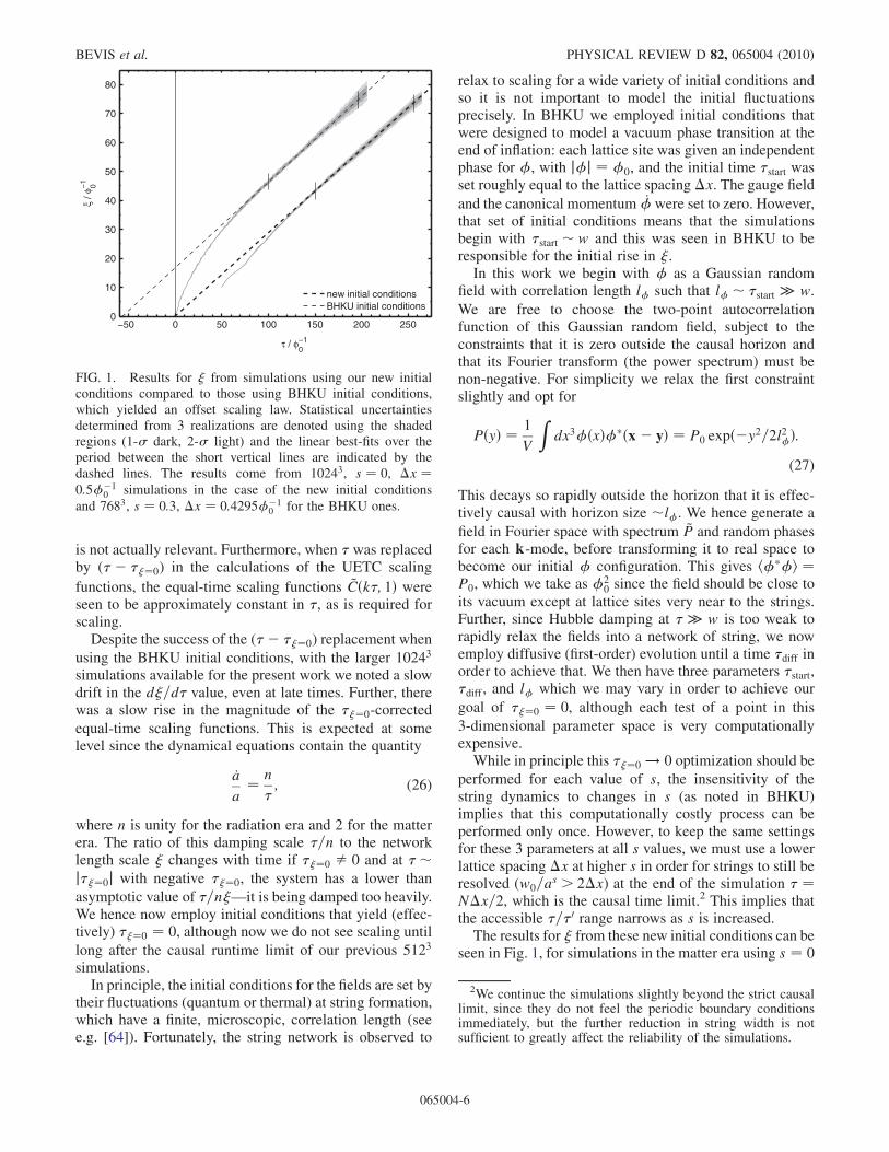
simulation size of 5123, which is about the minimumrequired to study a scaling network of strings. We thereforewere forced to be content with initial conditions thatyielded not � / � but � / ð�� ��¼0Þ, as shown in Fig. 1,

were ��¼0 is negative. That is, at early times string decay

occurred more quickly than scaling would have predictedand � increased rapidly, but then stabilized to an approxi-mately constant d�=d� once � * 40w (where w � ��1

0

but is slowly decreasing with � in the s ¼ 0:3 simulationfor which BHKU-style results are plotted). As can beseen in the figure, this rapid increase aids the creation ofan approximately scaling network for simulations thatare causally limited to small times, albeit scaling with(�� ��¼0) rather than �. Fortunately, at times of cosmo-

logical interest we have � ��¼0 and therefore this offset

1We measure L by detecting the lattice grid-squares aroundwhich the phase � has a net winding (using the gauge-invariantmethod of Ref. [62]) and then we approximately reconstruct thestring path as a collection of perpendicular segments of length�x passing through these squares. We then apply the Scherrer-Vilenkin correction factor of =6 [63] in order to approximatelyaccount for overestimate due to representing a smooth path byperpendicular segments (see Ref. [50] for more discussion).

CMB POWER SPECTRA FROM COSMIC STRINGS: . . . PHYSICAL REVIEW D 82, 065004 (2010)

065004-5

is not actually relevant. Furthermore, when � was replacedby (�� ��¼0) in the calculations of the UETC scaling

functions, the equal-time scaling functions ~Cðk�; 1Þ wereseen to be approximately constant in �, as is required forscaling.

Despite the success of the (�� ��¼0) replacement when

using the BHKU initial conditions, with the larger 10243

simulations available for the present work we noted a slowdrift in the d�=d� value, even at late times. Further, therewas a slow rise in the magnitude of the ��¼0-corrected

equal-time scaling functions. This is expected at somelevel since the dynamical equations contain the quantity

_a

a¼ n

�; (26)

where n is unity for the radiation era and 2 for the matterera. The ratio of this damping scale �=n to the networklength scale � changes with time if ��¼0 � 0 and at �j��¼0j with negative ��¼0, the system has a lower than

asymptotic value of �=n�—it is being damped too heavily.We hence now employ initial conditions that yield (effec-tively) ��¼0 ¼ 0, although now we do not see scaling until

long after the causal runtime limit of our previous 5123

simulations.In principle, the initial conditions for the fields are set by

their fluctuations (quantum or thermal) at string formation,which have a finite, microscopic, correlation length (seee.g. [64]). Fortunately, the string network is observed to

relax to scaling for a wide variety of initial conditions andso it is not important to model the initial fluctuationsprecisely. In BHKU we employed initial conditions thatwere designed to model a vacuum phase transition at theend of inflation: each lattice site was given an independentphase for �, with j�j ¼ �0, and the initial time �start wasset roughly equal to the lattice spacing �x. The gauge field

and the canonical momentum _�were set to zero. However,that set of initial conditions means that the simulationsbegin with �start w and this was seen in BHKU to beresponsible for the initial rise in �.In this work we begin with � as a Gaussian random

field with correlation length l� such that l� �start w.

We are free to choose the two-point autocorrelationfunction of this Gaussian random field, subject to theconstraints that it is zero outside the causal horizon andthat its Fourier transform (the power spectrum) must benon-negative. For simplicity we relax the first constraintslightly and opt for

PðyÞ ¼ 1

V

Zdx3�ðxÞ��ðx� yÞ ¼ P0 expð�y2=2l2�Þ:

(27)

This decays so rapidly outside the horizon that it is effec-tively causal with horizon size l�. We hence generate a

field in Fourier space with spectrum ~P and random phasesfor each k-mode, before transforming it to real space tobecome our initial � configuration. This gives h���i ¼P0, which we take as �2

0 since the field should be close to

its vacuum except at lattice sites very near to the strings.Further, since Hubble damping at � w is too weak torapidly relax the fields into a network of string, we nowemploy diffusive (first-order) evolution until a time �diff inorder to achieve that. We then have three parameters �start,�diff , and l� which we may vary in order to achieve our

goal of ��¼0 ¼ 0, although each test of a point in this

3-dimensional parameter space is very computationallyexpensive.While in principle this ��¼0 ! 0 optimization should be

performed for each value of s, the insensitivity of thestring dynamics to changes in s (as noted in BHKU)implies that this computationally costly process can beperformed only once. However, to keep the same settingsfor these 3 parameters at all s values, we must use a lowerlattice spacing �x at higher s in order for strings to still beresolved (w0=a

s > 2�x) at the end of the simulation � ¼N�x=2, which is the causal time limit.2 This implies thatthe accessible �=�0 range narrows as s is increased.The results for � from these new initial conditions can be

seen in Fig. 1, for simulations in the matter era using s ¼ 0

−50 0 50 100 150 200 2500

10

20

30

40

50

60

70

80

τ / φ0−1

ξ / φ

0−1

new initial conditionsBHKU initial conditions

FIG. 1. Results for � from simulations using our new initialconditions compared to those using BHKU initial conditions,which yielded an offset scaling law. Statistical uncertaintiesdetermined from 3 realizations are denoted using the shadedregions (1- dark, 2- light) and the linear best-fits over theperiod between the short vertical lines are indicated by thedashed lines. The results come from 10243, s ¼ 0, �x ¼0:5��1

0 simulations in the case of the new initial conditions

and 7683, s ¼ 0:3, �x ¼ 0:4295��10 for the BHKU ones.

2We continue the simulations slightly beyond the strict causallimit, since they do not feel the periodic boundary conditionsimmediately, but the further reduction in string width is notsufficient to greatly affect the reliability of the simulations.

BEVIS et al. PHYSICAL REVIEW D 82, 065004 (2010)

065004-6

(with a ¼ 1, � ¼ 2 and e ¼ 1 during diffusive evolutionand �x ¼ 0:5��1

0 ). Further, we show from the same simu-

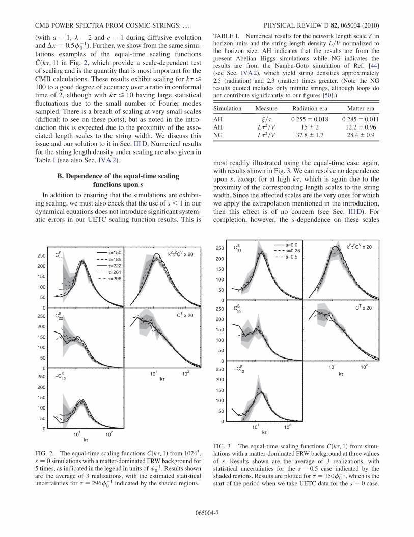
lations examples of the equal-time scaling functions~Cðk�; 1Þ in Fig. 2, which provide a scale-dependent testof scaling and is the quantity that is most important for theCMB calculations. These results exhibit scaling for k� &100 to a good degree of accuracy over a ratio in conformaltime of 2, although with k� & 10 having large statisticalfluctuations due to the small number of Fourier modessampled. There is a breach of scaling at very small scales(difficult to see on these plots), but as noted in the intro-duction this is expected due to the proximity of the asso-ciated length scales to the string width. We discuss thisissue and our solution to it in Sec. III D. Numerical resultsfor the string length density under scaling are also given inTable I (see also Sec. IVA2).

B. Dependence of the equal-time scalingfunctions upon s

In addition to ensuring that the simulations are exhibit-ing scaling, we must also check that the use of s < 1 in ourdynamical equations does not introduce significant system-atic errors in our UETC scaling function results. This is

most readily illustrated using the equal-time case again,with results shown in Fig. 3. We can resolve no dependenceupon s, except for at high k�, which is again due to theproximity of the corresponding length scales to the stringwidth. Since the affected scales are the very ones for whichwe apply the extrapolation mentioned in the introduction,then this effect is of no concern (see Sec. III D). Forcompletion, however, the s-dependence on these scales

0

50

100

150

200

250 CS11

τ=150τ=185τ=222τ=261τ=296

0

50

100

150

200

250 CS22

101

102

0

50

100

150

200

250

kτ

−CS12

k2τ2CV x 20

101

102

kτ

CT x 20

FIG. 2. The equal-time scaling functions ~Cðk�; 1Þ from 10243,s ¼ 0 simulations with a matter-dominated FRW background for5 times, as indicated in the legend in units of��1

0 . Results shown

are the average of 3 realizations, with the estimated statisticaluncertainties for � ¼ 296��1

0 indicated by the shaded regions.

TABLE I. Numerical results for the network length scale � inhorizon units and the string length density L=V normalized tothe horizon size. AH indicates that the results are from thepresent Abelian Higgs simulations while NG indicates theresults are from the Nambu-Goto simulation of Ref. [44](see Sec. IVA2), which yield string densities approximately2.5 (radiation) and 2.3 (matter) times greater. (Note the NGresults quoted includes only infinite strings, although loops donot contribute significantly to our figures [50].)

Simulation Measure Radiation era Matter era

AH �=� 0:255� 0:018 0:285� 0:011AH L�2=V 15� 2 12:2� 0:96NG L�2=V 37:8� 1:7 28:4� 0:9

0

50

100

150

200

250 CS11

s=0.0s=0.25s=0.5

0

50

100

150

200

250 CS22

101

102

0

50

100

150

200

250

kτ

−CS12

k2τ2CV x 20

101

102

kτ

CT x 20

FIG. 3. The equal-time scaling functions ~Cðk�; 1Þ from simu-lations with a matter-dominated FRW background at three valuesof s. Results shown are the average of 3 realizations, withstatistical uncertainties for the s ¼ 0:5 case indicated by theshaded regions. Results are plotted for � ¼ 150��1

0 , which is the

start of the period when we take UETC data for the s ¼ 0 case.

CMB POWER SPECTRA FROM COSMIC STRINGS: . . . PHYSICAL REVIEW D 82, 065004 (2010)

065004-7

can be explained as follows. The higher s, the more rapidthe reduction in comoving string width during the Hubblephase and therefore the attenuation of small scale power(see Sec. III D) manifests itself at higher k�. Hence thes ¼ 0 case yields lower results at the highest-plotted k�values.

Since s ¼ 0 simulations enable the greatest range in�=�0 under scaling, while accurately matching the dynam-ics seen at higher s values, our final CMB results willbe based upon s ¼ 0 simulations and we will limit our

remaining discussion in this article to simulations at thisvalue of s.

C. UETC scaling function results and decoherence

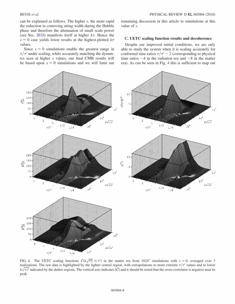
Despite our improved initial conditions, we are onlyable to study the system when it is scaling accurately forconformal time ratios �=�0 2 (corresponding to physicaltime ratios 4 in the radiation era and 8 in the matterera). As can be seen in Fig. 4 this is sufficient to map out

FIG. 4. The UETC scaling functions ~Cðk ffiffiffiffiffiffi��

p; �=�0Þ in the matter era from 10243 simulations with s ¼ 0, averaged over 3

realizations. The raw data is highlighted by the lighter central region, with extrapolations to more extreme �=�0 values and to lower

kffiffiffiffiffiffiffi��0

pindicated by the darker regions. The vertical axis indicates j ~Cj and it should be noted that the cross-correlator is negative near its

peak.

BEVIS et al. PHYSICAL REVIEW D 82, 065004 (2010)

065004-8

the important region of the UETCs, and to permit extrapo-lation in �=�0 as explained below. It can be seen that theautocorrelator scaling functions peak for � ¼ �0 and decayfor unequal times, with decay occurring for �=�0 ratios thatdeviate only slightly from one if k

ffiffiffiffiffiffiffi��0

pis large but more

slowly on superhorizon scales. In the cross-correlation case~CS12, this is broadly true but the peak is noticeably offset on

superhorizon scales.This behavior can be considered in more detail via the

coherence function, which we also use for �=�0 extra-polation. We define this function as follows in order to

remove the equal-time k� dependence from the unequal-time results:

~Dðkffiffiffiffiffiffiffi��0

p; �=�0Þ ¼

~Cðk ffiffiffiffiffiffiffi��0

p; �=�0Þffiffiffiffiffiffiffiffiffiffiffiffiffiffiffiffiffiffiffiffiffiffiffiffiffiffiffiffiffiffiffiffiffiffiffiffiffiffi

j ~Cðk�; 1Þ ~Cðk�0; 1Þjq ; (28)

where the modulus in the square root is relevant only for~CS12. This has the attractive feature of being equal to �1 at

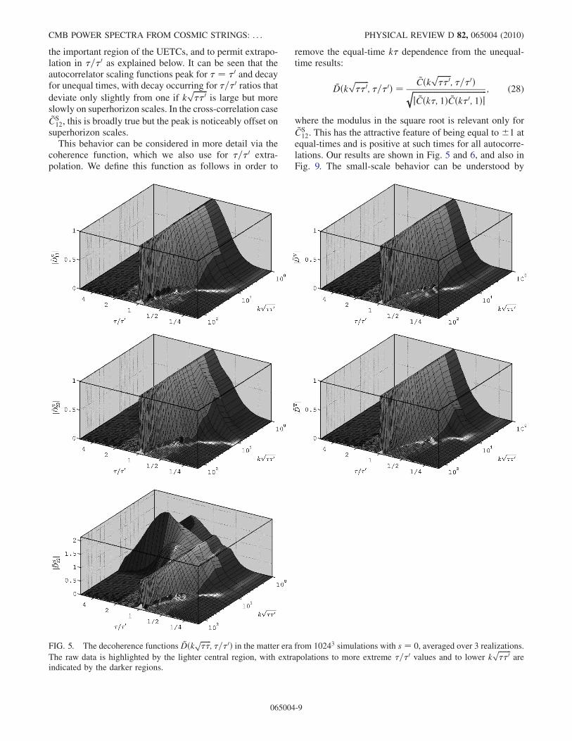
equal-times and is positive at such times for all autocorre-lations. Our results are shown in Fig. 5 and 6, and also inFig. 9. The small-scale behavior can be understood by

FIG. 5. The decoherence functions ~Dðk ffiffiffiffiffiffi��

p; �=�0Þ in the matter era from 10243 simulations with s ¼ 0, averaged over 3 realizations.

The raw data is highlighted by the lighter central region, with extrapolations to more extreme �=�0 values and to lower kffiffiffiffiffiffiffi��0

pare

indicated by the darker regions.

CMB POWER SPECTRA FROM COSMIC STRINGS: . . . PHYSICAL REVIEW D 82, 065004 (2010)

065004-9

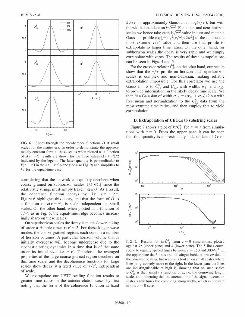
considering that the network can quickly decohere whencoarse grained on subhorizon scales 1=k � � since therelativistic strings must simply travel 2=k. As a result,the coherence function decays by jk�� k�0j 2.Figure 6 highlights this decay, and that the form of ~D asa function of kð�� �0Þ is scale independent on smallscales. On the other hand, when plotted as a function of�=�0, as in Fig. 5, the equal-time ridge becomes increas-ingly sharp on these scales.

On superhorizon scales the decay is much slower, takingof order a Hubble time: �=�0 2. For these longer wavemodes, the coarse-grained regions each contain a numberof horizon volumes. A particular horizon volume that isinitially overdense will become underdense due to thestochastic string dynamics in a time that is of the sameorder its initial size, i.e. �0. Therefore, the averagedproperties of the large coarse-grained region decohere onthis time scale, and the decoherence functions for largescales show decay at a fixed value of �=�0, independentof scale.

We extrapolate our UETC scaling function results togreater time ratios in the autocorrelation cases by firstnoting that the form of the coherence function at fixed

kffiffiffiffiffiffiffi��0

pis approximately Gaussian in logð�=�0Þ, but with

the width dependent on kffiffiffiffiffiffiffi��0

p. For super- and near-horizon

scales we hence take each kffiffiffiffiffiffiffi��0

pvalue in turn and match a

Gaussian profile exp½�log2ð�=�0Þ=22� to the data at themost extreme �=�0 value and then use that profile toextrapolate to larger time ratios. On the other hand, forsubhorizon scales the decay is very rapid and we simplyextrapolate with zeros. The results of these extrapolationscan be seen in Figs. 4 and 5.

For the cross correlator ~CS12 on the other hand, our results

show that the �=�0-profile on horizon and superhorizonscales is complex and non-Gaussian, making reliableextrapolation impossible. For this correlator we use the

Gaussian fits to ~CS11 and ~CS

22, with widths 11 and 22,to provide information on the likely decay time scale. Wethen fit a Gaussian of width 12 ¼ ð11 þ 22Þ=2 but withfree mean and normalization to the ~CS

12 data from themost extreme time ratios, and then employ that to yieldextrapolation.

D. Extrapolation of UETCs to substring scales

Figure 7 shows a plot of k� ~CS11 for �

0 ¼ � from simula-tions with s ¼ 0. From the upper pane it can be seenthat this quantity is approximately independent of k� on

0

0.5

1 DS11

5075100

0

0.5

1 DS22

−10 0 10

0

0.5

1

k(τ−τ’)

−DS12

DV

−10 0 10

k(τ−τ’)

DT

FIG. 6. Slices through the decoherence functions ~D at smallscales for the matter era. In order to demonstrate the approxi-mately constant form at these scales when plotted as a functionof kð�� �0Þ, results are shown for the three values kð�þ �0Þ=2indicated by the legend. The latter quantity is perpendicular tokð�� �0Þ in the k�� k�0 plane (see also Fig. 9) and simplifies tok� for the equal-time case.

101

102

103

100

102

104

kτ C

S 11(k

τ,kτ

)

kτ

10−1

100

101

100

102

104

kτ C

S 11(k

τ,kτ

)

k / φ0

FIG. 7. Results for k� ~CS11 from s ¼ 0 simulations, plotted

against k� (upper pane) and k (lower pane). The 5 lines corre-spond to equally spaced times between � ¼ 150 and 300��1

0 . In

the upper pane the 5 lines are indistinguishable at low k� due tothe observed scaling, but scaling is broken on small scales wherelines progressively move to the right. In the lower pane the linesare indistinguishable at high k, showing that on such scalesk� ~CS

11 is then simply a function of k, i.e. the comoving lengthscale, and indicating that the attenuation of the signal occurs onscales a few times the comoving string width, which is constantin this s ¼ 0 case.

BEVIS et al. PHYSICAL REVIEW D 82, 065004 (2010)

065004-10

subhorizon scales until k� 200 at the earliest timeshown or until about k� 400 at the latest time plotted.

The plateau highlights an important point: that ~CS11 drops

off as � 1=k� on subhorizon scales, which matches ourbasic expectations as well as similar measures from NGsimulations [65]. However, on smaller scales there is asudden attenuation of power, and at a k� value that isincreasing with time. The lower pane clarifies the laterby replotting this against k rather than k�, showing thatthis is occurring at a fixed comoving scale of k � 2�0.This corresponds to a few times the string width, which is afixed comoving width in this s ¼ 0 simulation.

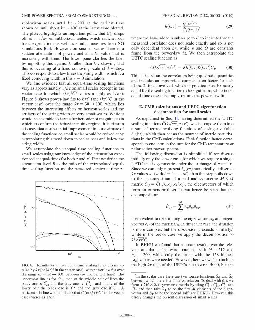
We find evidence that all equal-time scaling functionsvary as approximately 1=k� on small scales (except in the

vector case for which ðk�Þ2 ~CV varies roughly as 1=k�).

Figure 8 shows power-law fits to k� ~C (and ðk�Þ3 ~C in thevector case) over the range k� ¼ 30 ! 100, which liesbetween the interesting effects on horizon scales and theartifacts of the string width on very small scales. While itwould be desirable to have a further order of magnitude viawhich to confirm the behavior in this regime, it is clear inall cases that a substantial improvement in our estimate ofthe scaling functions on small scales would be arrived at byextrapolating this trend down to scales near and below thestring width.

We extrapolate the unequal time scaling functions tosmall scales using our knowledge of the attenuation expe-rienced at equal-times for both � and �0. First we define theattenuation level R as the ratio of the extrapolated equal-time scaling function and the measured version at time �:

Rðk; �Þ ¼ Qðk�Þ�p

~C�ðk�; 1Þ; (29)

where we have added a subscript to ~C to indicate that themeasured correlator does not scale exactly and so is notonly dependent upon k�, while p and Q are constantsfound from the power-law fit. We then extrapolate theUETC scaling function as

~Cðkffiffiffiffiffiffiffi��0

p; �=�0Þ ¼

ffiffiffiffiffiffiffiffiffiffiffiffiffiffiffiffiffiffiffiffiffiffiffiffiffiffiffiffiffiffiRðk; �ÞRðk; �0Þ

p~C�: (30)

This is based on the correlators being quadratic quantitiesand includes an appropriate compensation factor for eachof the 2 times involved, which in practice must be nearlyequal for the scaling function to be significant, while in theequal-time case this simply returns the power-law fit.

E. CMB calculations and UETC eigenfunctiondecomposition for small scales

As explained in Sec. II, having determined the UETC

scaling functions ~Cðk ffiffiffiffiffiffiffi��0

p; �=�0Þ, we decompose them into

a sum of terms involving functions of a single variable~cnðk�Þ, which then act as the sources of metric perturba-tions in the CMB calculations. Each function hence corre-sponds to one term in the sum for the CMB temperature orpolarization power spectra.The following discussion is simplified if we discuss

initially only the tensor case, for which we require a singleUETC that is symmetric under the exchange of � and �0.Since we can only represent ~cnðk�Þ numerically at discretek� values �i (with i ¼ 1; . . . ;M), then this step boils downto the decomposition of a real and symmetric M�M

matrix ~Cij ¼ ~Cð ffiffiffiffiffiffiffiffiffiffi�i�j

p; �i=�jÞ, the eigenvectors of which

form an orthonormal set. It can hence be seen that thedecomposition:

~C ij ¼XMn¼1

�n~cni~cnj; (31)

is equivalent to determining the eigenvalues �n and eigen-

vectors ~cni of the matrix ~Cij. In the scalar case, the situation

is more complex but the discussion proceeds similarly,3

while in the vector case we apply the decomposition to

k2ffiffiffiffiffiffiffi��0

p~C.

In BHKU we found that accurate results over the rele-vant angular scales were obtained with M ¼ 512 and�M ¼ 200, while only the terms with the 128 highestj�nj values were needed. However, here we wish to includethe high-k� tails of the UETCs out to k� 5000, but the

102

103

102

103

(kτ)

C

or

(kτ)

3 C

kτ

FIG. 8. Results for all five equal-time scaling functions multi-plied by k� [or ðk�Þ3 in the vector case], with power-law fits overthe range k� ¼ 50 ! 100 (between the two vertical lines). Theuppermost line is for ~CS

11, then of the middle pair of lines theblack one is ~CS

22 and the gray one is j ~CS12j, and finally of the

lower pair the black one is ~CV and the gray one if ~CT. Ahorizontal fit line would indicate that ~C (or ðk�Þ2 ~CV in the vectorcase) varies as 1=k�.

3In the scalar case there are two source functions ~S� and ~S�between which there is a finite correlation. To deal with this weform a 2M� 2M symmetric matrix by tiling ~CS

11,~CS12,

~CS21 and

~CS22 and then take ~S� to be the first M elements of the eigen-

vector and ~S� to be the second half (see BHKU). However, thisbarely changes the present discussion of small scales

CMB POWER SPECTRA FROM COSMIC STRINGS: . . . PHYSICAL REVIEW D 82, 065004 (2010)

065004-11

narrow width of the equal-time ridge requires �� � 1 andhence we would requireM 5000. Additionally, the smallamplitude of the tails implies that their signal is likely to becontained in eigenvectors with very low eigenvalues, andtherefore we would need to include all terms in our CMBcalculations. Because of the nature of the sources, eachEinstein-Boltzmann integration is much slower than thecorresponding primordially-seeded calculation requiredfor CMB predictions from inflation and hence this processwould be particularly time consuming. Further, the contri-butions to the CMB power spectrum in our target range2 � ‘ � 4000 from extremely high k� are minor, whileour knowledge of the UETCs on such scales is only viathe above power-law extrapolations.

We proceed instead by performing the decomposition insuch way that each ‘‘eigenvector’’ is localized in k�, sincewe then have an immediate understanding of how itcontributes to the CMB power spectra. First, we arrangefor all of the dominant horizon and superhorizon power(k� & 100) to be contained within a particular set ofeigenvectors, which then completely dominate the CMBtemperature power spectrum for multipoles ‘ & 1000, buttheir contributions decay for smaller angular scales.Second, the simple form of the UETC scaling functionson subhorizon scales allows us to obtain a knowledge ofthe CMB contributions from extremely high k� values bycombining our calculations for moderate k� values withapproximate scaling laws, as explained momentarily.

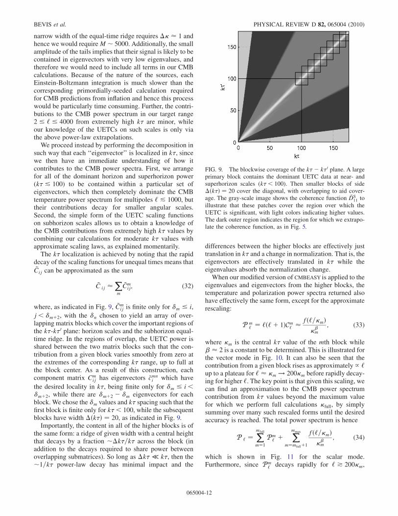
The k� localization is achieved by noting that the rapiddecay of the scaling functions for unequal times means that~Cij can be approximated as the sum

~C ij �Xm

~Cmij; (32)

where, as indicated in Fig. 9, ~Cmij is finite only for �m � i,

j < �mþ2, with the �n chosen to yield an array of over-lapping matrix blocks which cover the important regions ofthe k�-k�0 plane: horizon scales and the subhorizon equal-time ridge. In the regions of overlap, the UETC power isshared between the two matrix blocks such that the con-tribution from a given block varies smoothly from zero atthe extremes of the corresponding k� range, up to full atthe block center. As a result of this construction, eachcomponent matrix Cm

ij has eigenvectors ~cmni which have

the desired locality in k�, being finite only for �m � i <�mþ2, while there are �mþ2 � �m eigenvectors for eachblock. We chose the �m values and k� spacing such that thefirst block is finite only for k� < 100, while the subsequentblocks have width �ðk�Þ ¼ 20, as indicated in Fig. 9.

Importantly, the content in all of the higher blocks is ofthe same form: a ridge of given width with a central heightthat decays by a fraction �k�=k� across the block (inaddition to the decays required to share power betweenoverlapping submatrices). So long as �k� � k�, then the1=k� power-law decay has minimal impact and the

differences between the higher blocks are effectively justtranslation in k� and a change in normalization. That is, theeigenvectors are effectively translated in k� while theeigenvalues absorb the normalization change.When our modified version of CMBEASY is applied to the

eigenvalues and eigenvectors from the higher blocks, thetemperature and polarization power spectra returned alsohave effectively the same form, except for the approximaterescaling:

P m‘ ¼ ‘ð‘þ 1ÞCm‘ � fð‘=�mÞ

� m

; (33)

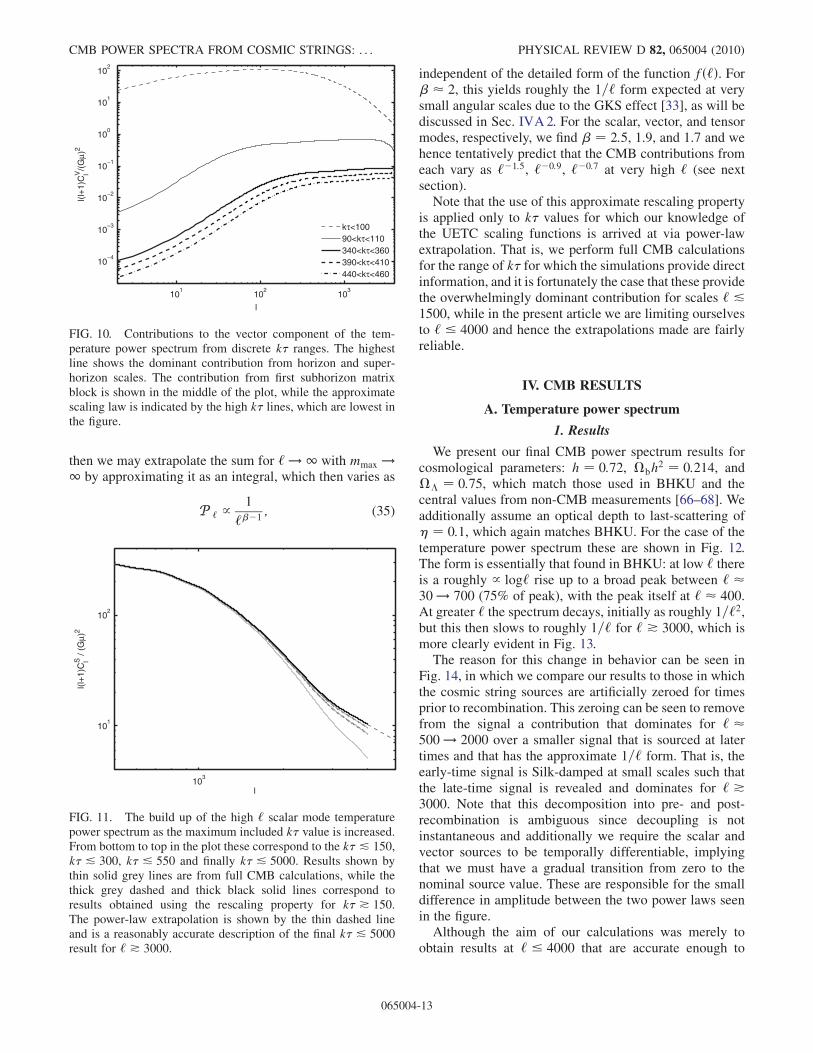
where �m is the central k� value of the mth block while � 2 is a constant to be determined. This is illustrated forthe vector mode in Fig. 10. It can also be seen that thecontribution from a given block rises as approximately / ‘up to a plateau for ‘ � �m ! 200�m before rapidly decay-ing for higher ‘. The key point is that given this scaling, wecan find an approximation to the CMB power spectrumcontribution from k� values beyond the maximum valuefor which we perform full calculations �full, by simplysumming over many such rescaled forms until the desiredaccuracy is reached. The total power spectrum is hence

P ‘ ¼Xmfull

m¼1

Pm‘ þ Xmmax

m¼mfullþ1

fð‘=�mÞ� m

; (34)

which is shown in Fig. 11 for the scalar mode.Furthermore, since Pm

‘ decays rapidly for ‘ * 200�m,

FIG. 9. The blockwise coverage of the k�� k�0 plane. A largeprimary block contains the dominant UETC data at near- andsuperhorizon scales (k� < 100). Then smaller blocks of side�ðk�Þ ¼ 20 cover the diagonal, with overlapping to aid cover-age. The gray-scale image shows the coherence function ~DS

11 to

illustrate that these patches cover the region over which theUETC is significant, with light colors indicating higher values.The dark outer region indicates the region for which we extrapo-late the coherence function, as in Fig. 5.

BEVIS et al. PHYSICAL REVIEW D 82, 065004 (2010)

065004-12

then we may extrapolate the sum for ‘ ! 1 with mmax !1 by approximating it as an integral, which then varies as

P ‘ / 1

‘ �1; (35)

independent of the detailed form of the function fð‘Þ. For � 2, this yields roughly the 1=‘ form expected at verysmall angular scales due to the GKS effect [33], as will bediscussed in Sec. IVA2. For the scalar, vector, and tensormodes, respectively, we find ¼ 2:5, 1.9, and 1.7 and wehence tentatively predict that the CMB contributions fromeach vary as ‘�1:5, ‘�0:9, ‘�0:7 at very high ‘ (see nextsection).Note that the use of this approximate rescaling property

is applied only to k� values for which our knowledge ofthe UETC scaling functions is arrived at via power-lawextrapolation. That is, we perform full CMB calculationsfor the range of k� for which the simulations provide directinformation, and it is fortunately the case that these providethe overwhelmingly dominant contribution for scales ‘ &1500, while in the present article we are limiting ourselvesto ‘ � 4000 and hence the extrapolations made are fairlyreliable.

IV. CMB RESULTS

A. Temperature power spectrum

1. Results

We present our final CMB power spectrum results forcosmological parameters: h ¼ 0:72, �bh

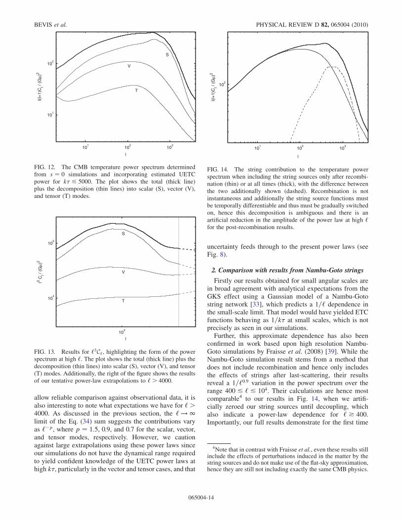
2 ¼ 0:214, and�� ¼ 0:75, which match those used in BHKU and thecentral values from non-CMB measurements [66–68]. Weadditionally assume an optical depth to last-scattering of� ¼ 0:1, which again matches BHKU. For the case of thetemperature power spectrum these are shown in Fig. 12.The form is essentially that found in BHKU: at low ‘ thereis a roughly / log‘ rise up to a broad peak between ‘ �30 ! 700 (75% of peak), with the peak itself at ‘ � 400.At greater ‘ the spectrum decays, initially as roughly 1=‘2,but this then slows to roughly 1=‘ for ‘ * 3000, which ismore clearly evident in Fig. 13.The reason for this change in behavior can be seen in

Fig. 14, in which we compare our results to those in whichthe cosmic string sources are artificially zeroed for timesprior to recombination. This zeroing can be seen to removefrom the signal a contribution that dominates for ‘ �500 ! 2000 over a smaller signal that is sourced at latertimes and that has the approximate 1=‘ form. That is, theearly-time signal is Silk-damped at small scales such thatthe late-time signal is revealed and dominates for ‘ *3000. Note that this decomposition into pre- and post-recombination is ambiguous since decoupling is notinstantaneous and additionally we require the scalar andvector sources to be temporally differentiable, implyingthat we must have a gradual transition from zero to thenominal source value. These are responsible for the smalldifference in amplitude between the two power laws seenin the figure.Although the aim of our calculations was merely to

obtain results at ‘ � 4000 that are accurate enough to

101

102

103

10−4

10−3

10−2

10−1

100

101

102

l

l(l+

1)C

lV/(

Gµ)

2

kτ<10090<kτ<110340<kτ<360390<kτ<410440<kτ<460

FIG. 10. Contributions to the vector component of the tem-perature power spectrum from discrete k� ranges. The highestline shows the dominant contribution from horizon and super-horizon scales. The contribution from first subhorizon matrixblock is shown in the middle of the plot, while the approximatescaling law is indicated by the high k� lines, which are lowest inthe figure.

103

101

102

l

l(l+

1)C

S l /

(Gµ)

2

FIG. 11. The build up of the high ‘ scalar mode temperaturepower spectrum as the maximum included k� value is increased.From bottom to top in the plot these correspond to the k� & 150,k� & 300, k� & 550 and finally k� & 5000. Results shown bythin solid grey lines are from full CMB calculations, while thethick grey dashed and thick black solid lines correspond toresults obtained using the rescaling property for k� * 150.The power-law extrapolation is shown by the thin dashed lineand is a reasonably accurate description of the final k� & 5000result for ‘ * 3000.

CMB POWER SPECTRA FROM COSMIC STRINGS: . . . PHYSICAL REVIEW D 82, 065004 (2010)

065004-13

allow reliable comparison against observational data, it isalso interesting to note what expectations we have for ‘ >4000. As discussed in the previous section, the ‘ ! 1limit of the Eq. (34) sum suggests the contributions varyas ‘�p, where p ¼ 1:5, 0.9, and 0.7 for the scalar, vector,and tensor modes, respectively. However, we cautionagainst large extrapolations using these power laws sinceour simulations do not have the dynamical range requiredto yield confident knowledge of the UETC power laws athigh k�, particularly in the vector and tensor cases, and that

uncertainty feeds through to the present power laws (seeFig. 8).

2. Comparison with results from Nambu-Goto strings

Firstly our results obtained for small angular scales arein broad agreement with analytical expectations from theGKS effect using a Gaussian model of a Nambu-Gotostring network [33], which predicts a 1=‘ dependence inthe small-scale limit. That model would have yielded ETCfunctions behaving as 1=k� at small scales, which is notprecisely as seen in our simulations.Further, this approximate dependence has also been

confirmed in work based upon high resolution Nambu-Goto simulations by Fraisse et al. (2008) [39]. While theNambu-Goto simulation result stems from a method thatdoes not include recombination and hence only includesthe effects of strings after last-scattering, their resultsreveal a 1=‘0:9 variation in the power spectrum over therange 400 & ‘ & 104. Their calculations are hence mostcomparable4 to our results in Fig. 14, when we artifi-cially zeroed our string sources until decoupling, whichalso indicate a power-law dependence for ‘ * 400.Importantly, our full results demonstrate for the first time

101

102

103

101

102

S

V

T

l

l(l+

1)C

l / (G

µ)2

FIG. 12. The CMB temperature power spectrum determinedfrom s ¼ 0 simulations and incorporating estimated UETCpower for k� & 5000. The plot shows the total (thick line)plus the decomposition (thin lines) into scalar (S), vector (V),and tensor (T) modes.

103

104

105

S

V

T

l

l3 Cl /

(Gµ)

2

FIG. 13. Results for ‘3C‘, highlighting the form of the powerspectrum at high ‘. The plot shows the total (thick line) plus thedecomposition (thin lines) into scalar (S), vector (V), and tensor(T) modes. Additionally, the right of the figure shows the resultsof our tentative power-law extrapolations to ‘ > 4000.

101

102

103

102

l

l(l+

1)C

l / (G

µ)2

FIG. 14. The string contribution to the temperature powerspectrum when including the string sources only after recombi-nation (thin) or at all times (thick), with the difference betweenthe two additionally shown (dashed). Recombination is notinstantaneous and additionally the string source functions mustbe temporally differentiable and thus must be gradually switchedon, hence this decomposition is ambiguous and there is anartificial reduction in the amplitude of the power law at high ‘for the post-recombination results.

4Note that in contrast with Fraisse et al., even these results stillinclude the effects of perturbations induced in the matter by thestring sources and do not make use of the flat-sky approximation,hence they are still not including exactly the same CMB physics.

BEVIS et al. PHYSICAL REVIEW D 82, 065004 (2010)

065004-14

at which angular scales this � 1=‘ dependence is valid,namely ‘ * 3000—scales finer than a few arc minutes.

At angular scales near the peak of the spectrum(‘ 400) there are no recently published results fromNambu-Goto simulations against which we can compareour results, with Contaldi et al. (1999) [40] providing theonly example of such work. However, this employedMinkowski space-time simulations plus now outdated cos-mological parameters and therefore a detailed comparisonis not appropriate. The basic form of our spectrum is ingood agreement with their results, although their powerspectrum shows a shift to higher ‘ compared to thosepresented here. Further, their results suggest that Nambu-Goto networks yield CMB predictions with a larger overallnormalization. This is also seen by comparing to powerspectra calculated from FRW Nambu-Goto simulationsand modern cosmological parameters, but which are validonly for discrete multipole ranges (and miss the ‘ 400peak) [38,69]. Nambu-Goto strings would require G� �0:7� 10�6 in order to fit observations at ‘ < 10 [38],while we would require G� ¼ 1:8� 10�6 to match theWMAP5 result at ‘ ¼ 10. This is not unexpected given thesimulation results and, as shown in Table I, Nambu-Gotocalculations yield higher string densities than field theo-retic ones, raising the power spectrum normalization andshifting power to smaller scales. We believe this densitydifference is because field theory simulations provide adecay channel, namely, radiative decay, which is not in-cluded the Nambu-Goto codes. Despite this, the Fraisseet al. result for ‘ð‘þ 1ÞC‘=ðG�Þ2 at ‘ ¼ 4000 is � 25,which compares favorably to our result of 20 at this multi-pole. This may be due to ambiguities associated with theirnoninclusion of recombination rather than a real agreementin the amplitude of the power law.

As discussed in the introduction, the USM is a computa-tionally cheap means of estimating the CMB power spec-trum, and this has also been used to study the stringcontribution at sub-WMAP angular scales with the USMparameters set to approximate a Nambu-Goto network.The published work [43] highlighted a 1=‘2 dependencenear ‘ 2000, but a more recent look at greater ‘prompted by our results does indeed reveal an approxi-mately 1=‘ variation in the USM power spectrum above‘ 3000 [70].

3. Comparison with the contribution from inflation

It is of course useful to compare the cosmic string powerspectrum with that from inflation, to which it should beadded.5 This comparison is eased if we give the stringcontribution an artificially high normalization such that it

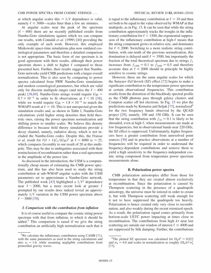
is equal to the inflationary contribution at ‘ ¼ 10 and thenset both to be equal to the value observed byWMAP at thatmultipole, as in Fig. 15. It can be seen that while the stringcontribution approximately tracks the troughs in the infla-tionary contribution for ‘ < 1500, the exponential suppres-sion of the inflationary contribution at high-‘ means thatthe string component grows in relative size, and dominatesfor ‘ * 2000. Switching to a more realistic string contri-bution, with one-tenth of the previous normalization, thisdomination is delayed until ‘ � 3500, but importantly thefraction of the total theoretical spectrum due to strings f‘increases from f1500 � 0:1 to f3500 ¼ 0:5 and thereforeaccurate data at ‘ * 2000 should in principle be highlysensitive to cosmic strings.However, these are the same angular scales for which

the Sunyaev-Zel’dovich (SZ) effect [72] begins to make asignificant contribution to the temperature power spectrumat certain observational frequencies. This contributionresults from the distortion of the blackbody spectral profileas the CMB photons pass through galaxy clusters andCompton scatter off hot electrons. In Fig. 15 we plot thepredictions made by Komatsu and Seljak [73], normalized6

for the two frequency bands observed by the QUADproject [29], namely, 100 and 150 GHz. It can be seenthat the string contribution with f10 � 0:1 is likely to beshrouded, even at high ‘, when measurements are made atlow frequencies, but in observational bands near 220 GHz,the SZ effect is suppressed. Unfortunately, higher frequen-cies have a greater contribution from unresolved pointsources [30] and in practice observations at a number offrequencies will be required in order to understand thefrequency-dependent contributions and remove them toyield a high sensitivity to the frequency-independent cos-mic string component from temperature power spectrummeasurements alone.

B. Polarization power spectra

CMB polarization anisotropies differ from those fortemperature in that they are created almost exclusivelyat recombination. Since the polarization is caused byThompson scattering in the presence of a quadrupoleanisotropy, the universe must be ionized in order to createit, but with Thompson scattering still weak enough forit not to have suppressed the quadrupole too heavily.Polarization is hence created only very close to recombi-nation, and also weakly during the recent reionized epoch.As a result, the polarization signal comes primarily fromhorizon-scale UETC power impacting at times close torecombination. The contributions from high k� near lastscattering are outside our window of interest ‘ � 4000 andare suppressed by Silk damping. Further, the contributions

5We calculate the inflationary contribution using CAMB [71],with the same parameters as used in the string calculations andalso ns ¼ 1:0, while assuming negligible contributions fromprimordial gravity waves.

6The plotted SZ spectrum was calculated for �bh2 ¼ 0:023

and 8 ¼ 0:8 and scales in normalization as roughly ð�bhÞ278

[73].

CMB POWER SPECTRA FROM COSMIC STRINGS: . . . PHYSICAL REVIEW D 82, 065004 (2010)

065004-15

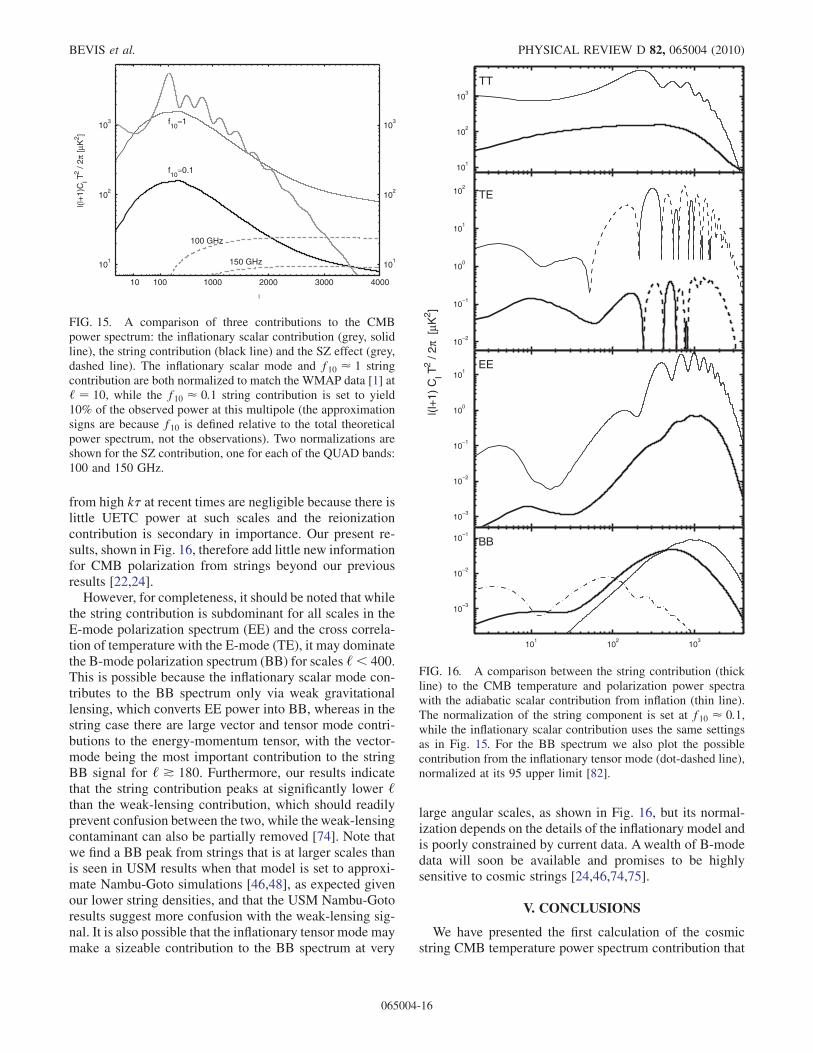
from high k� at recent times are negligible because there islittle UETC power at such scales and the reionizationcontribution is secondary in importance. Our present re-sults, shown in Fig. 16, therefore add little new informationfor CMB polarization from strings beyond our previousresults [22,24].

However, for completeness, it should be noted that whilethe string contribution is subdominant for all scales in theE-mode polarization spectrum (EE) and the cross correla-tion of temperature with the E-mode (TE), it may dominatethe B-mode polarization spectrum (BB) for scales ‘ < 400.This is possible because the inflationary scalar mode con-tributes to the BB spectrum only via weak gravitationallensing, which converts EE power into BB, whereas in thestring case there are large vector and tensor mode contri-butions to the energy-momentum tensor, with the vector-mode being the most important contribution to the stringBB signal for ‘ * 180. Furthermore, our results indicatethat the string contribution peaks at significantly lower ‘than the weak-lensing contribution, which should readilyprevent confusion between the two, while the weak-lensingcontaminant can also be partially removed [74]. Note thatwe find a BB peak from strings that is at larger scales thanis seen in USM results when that model is set to approxi-mate Nambu-Goto simulations [46,48], as expected givenour lower string densities, and that the USM Nambu-Gotoresults suggest more confusion with the weak-lensing sig-nal. It is also possible that the inflationary tensor mode maymake a sizeable contribution to the BB spectrum at very

large angular scales, as shown in Fig. 16, but its normal-ization depends on the details of the inflationary model andis poorly constrained by current data. Awealth of B-modedata will soon be available and promises to be highlysensitive to cosmic strings [24,46,74,75].

V. CONCLUSIONS

We have presented the first calculation of the cosmicstring CMB temperature power spectrum contribution that

1000 2000 3000 4000

101

102

103

l

10 100

101

102

103

l(l+

1)C

l T2 /

2π [µ

K2 ]

150 GHz

100 GHz

f10

≈0.1

f10

≈1

FIG. 15. A comparison of three contributions to the CMBpower spectrum: the inflationary scalar contribution (grey, solidline), the string contribution (black line) and the SZ effect (grey,dashed line). The inflationary scalar mode and f10 � 1 stringcontribution are both normalized to match the WMAP data [1] at‘ ¼ 10, while the f10 � 0:1 string contribution is set to yield10% of the observed power at this multipole (the approximationsigns are because f10 is defined relative to the total theoreticalpower spectrum, not the observations). Two normalizations areshown for the SZ contribution, one for each of the QUAD bands:100 and 150 GHz.

101

102

103

101

102

103

TT

101

102

103

10−2

10−1

100

101

102

TE

101

102

103

10−3

10−2

10−1

100

101

EE

101

102

103

10−3

10−2

10−1

BB

l(l+

1) C

l T2 /

2π [

µK2 ]

FIG. 16. A comparison between the string contribution (thickline) to the CMB temperature and polarization power spectrawith the adiabatic scalar contribution from inflation (thin line).The normalization of the string component is set at f10 � 0:1,while the inflationary scalar contribution uses the same settingsas in Fig. 15. For the BB spectrum we also plot the possiblecontribution from the inflationary tensor mode (dot-dashed line),normalized at its 95 upper limit [82].

BEVIS et al. PHYSICAL REVIEW D 82, 065004 (2010)

065004-16

is accurate over the multipole range ‘ ¼ 2 ! 4000, arange that encloses the scales probed by the Planck satellite(‘ ¼ 2 ! 2500) and additionally scales at which suborbi-tal data are becoming increasingly accurate. Further, weshow that at ‘ 3000 there is a knee in the power spectrumresult due to the exponential decay of the early time con-tribution at small angular scales, which then reveals thepost-recombination component. This late-time contribu-tion varies as roughly 1=‘, which is the basic expectationfor the GKS effect [33]. Our results yield values for thepower-law exponent for each of the scalar, vector andtensor contributions to the overall high-‘ behavior andcan, in principle, be used to estimate the temperaturecontribution from strings for ‘ > 4000. However thisextrapolation must be performed with caution since oursimulations do not have the dynamic range to yield thesepower laws with great confidence.

Our results indicate that the size of the cosmic stringsignal in the temperature power spectrum, relative to theadiabatic inflationary component, is roughly 10 timesgreater at ‘ � 3500 than it is at ‘ � 10 or ‘ � 400–1500and therefore small angular scales are particularly impor-tant for cosmic strings. While it is true that other con-tributions also become significant at small scales, forexample, the Sunyaev-Zel’dovich effect, such effects arefrequency dependent and hence can be identified and sub-tracted. Further, our results are not limited to temperatureanisotropies but include polarization also, which is of greatfuture importance for strings in the case of the B-mode. Wepresent a comparison of our temperature and polarizationresults to the latest data in a separate, shorter article [76].

Our simulations also yield greater knowledge of thescaling properties of Abelian Higgs string networks, withimprovements in the accuracy of results such as the scalingdensity and the UETCs. Additionally, we have measuredthe coherence function for Abelian Higgs strings for thefirst time, the form of which is important for calculations ofthis kind.

That our results stem from the Abelian Higgs modelmeans, of course, that they are not necessarily accurate for

cosmic superstrings (see e.g. [10] for a review). Thesesuperstrings may have intercommutation probabilities sig-nificantly lower than that for gauge strings and additionallymay form Y-shaped junctions, which do not form in theAbelian Higgs model for the parameters chosen here.While small-scale structure on the strings has been shownto lessen the impact of the intercommutation probability[77], the effect of Y-junctions on the network properties ishighly uncertain. Both effects are likely to increase thestring density and decrease the interstring distance,resulting in a shift of the peak in the CMB signal to greater‘ values. This may, therefore, enable superstrings to bedistinguished from conventional cosmic strings shoulda string component in the CMB be detected in futuredata.Finally, we note that the power spectrum is not a com-

plete statistical description of the anisotropies that wouldbe seeded by cosmic strings, since there would be a sig-nificant non-Gaussian character created by the GKS effect.Higher order moments such as the bispectrum, trispectrum,and skewness have been calculated [78–81], in addition torealizations of CMB maps [44,69]. While these calcula-tions are challenging and either do not include recombina-tion or are valid only for very limited multipole ranges,non-Gaussianity is an exciting channel for future cosmicstring constraint or detection.

ACKNOWLEDGMENTS

We acknowledge financial support from STFC (N. B.),the Swiss National Science Foundation (M.K.), theSpanish Consolider-Ingenio 2010 Programme CPAN(CSD2007-00042), and the Spanish Ministry of Scienceand Innovation FPA2009-10612 (J. U.). Numerical calcu-lations were performed using the U.K. National Cosmo-logy Supercomputer (COSMOS, supported by SGI/Intel,HEFCE, and STFC), the Imperial College HPC facilities,and the University of Sussex HPC Archimedes cluster.We thank Arttu Rajantie and Levon Pogosian for usefuldiscussions.

[1] M.R. Nolta et al. (WMAP), Astrophys. J. Suppl. Ser. 180,296 (2009).

[2] W. J. Percival et al., Mon. Not. R. Astron. Soc. 401, 2148(2010).

[3] N. Bevis, M. Hindmarsh, M. Kunz, and J. Urrestilla, Phys.Rev. Lett. 100, 021301 (2008).

[4] R. A. Battye, B. Garbrecht, and A. Moss, J. Cosmol.Astropart. Phys. 09 (2006) 007.

[5] A. A. Fraisse, J. Cosmol. Astropart. Phys. 03 (2007) 008.[6] M. Wyman, L. Pogosian, and I. Wasserman, Phys. Rev. D

72, 023513 (2005).

[7] A. Vilenkin and E. P. S. Shellard, Cosmic Strings andOther Topological Defects (Cambridge University Press,Cambridge, England, 1994).

[8] M. B. Hindmarsh and T.W. B. Kibble, Rep. Prog. Phys.58, 477 (1995).

[9] M. Sakellariadou, Lect. Notes Phys. 718, 247 (2007).[10] E. J. Copeland and T.W. B. Kibble, Proc. R. Soc. A 466,

623 (2010).[11] S. Sarangi and S. H.H. Tye, Phys. Lett. B 536, 185 (2002).[12] N. T. Jones, H. Stoica, and S.H. H. Tye, Phys. Lett. B 563,

6 (2003).

CMB POWER SPECTRA FROM COSMIC STRINGS: . . . PHYSICAL REVIEW D 82, 065004 (2010)

065004-17

[13] R. Jeannerot, J. Rocher, and M. Sakellariadou, Phys. Rev.D 68, 103514 (2003).

[14] T. Vachaspati and A. Achucarro, Phys. Rev. D 44, 3067(1991).

[15] M. Hindmarsh, Phys. Rev. Lett. 68, 1263 (1992).[16] A. Achucarro and T. Vachaspati, Phys. Rep. 327, 347

(2000).[17] A. Achucarro, P. Salmi, and J. Urrestilla, Phys. Rev. D 75,

121703 (2007).[18] U.-L. Pen, U. Seljak, and N. Turok, Phys. Rev. Lett. 79,

1611 (1997).[19] R. Durrer, M. Kunz, and A. Melchiorri, Phys. Rev. D 59,

123005 (1999).[20] N. Bevis, M. Hindmarsh, and M. Kunz, Phys. Rev. D 70,

043508 (2004).[21] M. Cruz, N. Turok, P. Vielva, E. Martinez-Gonzalez, and

M. Hobson, Science 318, 1612 (2007).[22] J. Urrestilla, N. Bevis, M. Hindmarsh, M. Kunz, and

A. R. Liddle, J. Cosmol. Astropart. Phys. 07 (2008) 010.[23] N. Bevis, M. Hindmarsh, M. Kunz, and J. Urrestilla, Phys.

Rev. D 75, 065015 (2007).[24] N. Bevis, M. Hindmarsh, M. Kunz, and J. Urrestilla, Phys.

Rev. D 76, 043005 (2007).[25] G. Hinshaw and others (WMAP), Astrophys. J. Suppl. Ser.

170, 288 (2007).[26] D. N. Spergel and others (WMAP), Astrophys. J. Suppl.

Ser. 170, 377 (2007).[27] J. L. Sievers et al. (CBI), arXiv:0901.4540.[28] C. L. Reichardt et al. (ACBAR), Astrophys. J. 694, 1200

(2009).[29] R. B. Friedman et al. (QUaD), Astrophys. J. 700, L187

(2009).[30] M. Lueker et al., Astrophys. J. 719, 1045 (2010).[31] J. Fowler et al. (The ACT), arXiv:1001.2934.[32] Planck satelite, ESA, http://www.rssd.esa.int/index.php?

project=Planck.[33] M. Hindmarsh, Astrophys. J. 431, 534 (1994).[34] T.W. B. Kibble, Nucl. Phys. B252, 227 (1985).[35] N. Kaiser and A. Stebbins, Nature (London) 310, 391

(1984).[36] A. Stebbins, Astrophys. J. 327, 584 (1988).[37] J. R. Gott, III, Astrophys. J. 288, 422 (1985).[38] M. Landriau and E. P. S. Shellard, Phys. Rev. D 69,

023003 (2004).[39] A. A. Fraisse, C. Ringeval, D.N. Spergel, and F. R.

Bouchet, Phys. Rev. D 78, 043535 (2008).[40] C. Contaldi, M. Hindmarsh, and J. Magueijo, Phys. Rev.

Lett. 82, 679 (1999).[41] A. Albrecht, R. A. Battye, and J. Robinson, Phys. Rev.

Lett. 79, 4736 (1997).[42] L. Pogosian and T. Vachaspati, Phys. Rev. D 60, 083504

(1999).[43] L. Pogosian, S. H.H. Tye, I. Wasserman, and M. Wyman J.

Cosmol. Astropart. Phys. 02 (2009) 013.[44] C. Ringeval, M. Sakellariadou, and F. Bouchet, J. Cosmol.

Astropart. Phys. 02 (2007) 023.[45] K. D. Olum and V. Vanchurin, Phys. Rev. D 75, 063521

(2007).[46] L. Pogosian and M. Wyman, Phys. Rev. D 77, 083509

(2008).

[47] R. Battye, B. Garbrecht, and A. Moss, Phys. Rev. D 81,123512 (2010).

[48] R. Battye and A. Moss, Phys. Rev. D 82, 023521(2010).

[49] G. Vincent, N.D. Antunes, and M. Hindmarsh, Phys. Rev.Lett. 80, 2277 (1998).

[50] M. Hindmarsh, S. Stuckey, and N. Bevis, Phys. Rev. D 79,123504 (2009).

[51] P. Bhattacharjee and G. Sigl, Phys. Rep. 327, 109 (2000).[52] U. Seljak and M. Zaldarriaga, Astrophys. J. 469, 437

(1996).[53] C. J. A. P. Martins and E. P. S. Shellard, Phys. Rev. D 73,

043515 (2006).[54] J. N. Moore, E. P. S. Shellard, and C. J. A. P. Martins, Phys.

Rev. D 65, 023503 (2001).[55] N. Turok, Phys. Rev. D 54, R3686 (1996).[56] M. Doran, J. Cosmol. Astropart. Phys. 10 (2005) 011.[57] R. Durrer and M. Kunz, Phys. Rev. D 57, R3199

(1998).[58] J.M. Bardeen, Phys. Rev. D 22, 1882 (1980).[59] R. Durrer, M. Kunz, and A. Melchiorri, Phys. Rep. 364, 1

(2002).[60] W. Hu and M. J. White, Phys. Rev. D 56, 596 (1997).[61] E. Bogomol’nyi, Sov. J. Nucl. Phys. 24, 449 (1976).[62] K. Kajantie, M. Karjalainen, M. Laine, J. Peisa, and

A. Rajantie, Phys. Lett. B 428, 334 (1998).[63] R. J. Scherrer and A. Vilenkin, Phys. Rev. D 58, 103501

(1998).[64] A. Rajantie, arXiv:hep-ph/0311262.[65] G. R. Vincent, M. Hindmarsh, and M. Sakellariadou, Phys.

Rev. D 55, 573 (1997).[66] W. L. Freedman et al., Astrophys. J. 553, 47 (2001).[67] D. Kirkman, D. Tytler, N. Suzuki, J.M. O’Meara, and

D. Lubin, Astrophys. J. Suppl. Ser. 149, 1 (2003).[68] R. A. Knop et al. (The Supernova Cosmology Project),

Astrophys. J. 598, 102 (2003).[69] M. Landriau and E. P. S. Shellard, arXiv:1004.2885.[70] L. Pogosian, S. H. H. Tye, I. Wasserman, and M. Wyman,

J. Cosmol. Astropart. Phys. 02 (2009) 013.[71] A. Lewis, A. Challinor, and A. Lasenby, Astrophys. J. 538,

473 (2000).[72] R. A. Sunyaev and Y.B. Zeldovich, Astrophys. Space Sci.

7, 3 (1970).[73] E. Komatsu and U. Seljak, Mon. Not. R. Astron. Soc. 336,

1256 (2002).[74] U. Seljak and A. Slosar, Phys. Rev. D 74, 063523 (2006).[75] J. Garcia-Bellido, R. Durrer, E. Fenu, D. G. Figueroa, and

M. Kunz, arXiv:1003.0299.[76] N. Bevis, M. Hindmarsh, M. Kunz, and J. Urrestilla

(unpublished).[77] A. Avgoustidis and E. P. S. Shellard, Phys. Rev. D 73,

041301 (2006).[78] M. Hindmarsh, C. Ringeval, and T. Suyama, Phys. Rev. D

80, 083501 (2009).[79] M. Hindmarsh, C. Ringeval, and T. Suyama, Phys. Rev. D

81, 063505 (2010).[80] D.M. Regan and E. P. S. Shellard, arXiv:0911.2491.[81] D. Yamauchi et al., J. Cosmol. Astropart. Phys. 05 (2010)

033.[82] E. Komatsu et al. (2010), arXiv:1001.4538.

BEVIS et al. PHYSICAL REVIEW D 82, 065004 (2010)

065004-18