PhotonsandtheElectromagneticField COPYRIGHTED MATERIAL · The foundations of a systematic quantum theory of fields were laid by Dirac in 1927 in his famous paper on ‘The Quantum

1

Photons and the Electromagnetic Field

1.1 Particles and Fields

The concept of photons as the quanta of the electromagnetic field dates back to the beginning

of the twentieth century. In order to explain the spectrum of black-body radiation, Planck, in

1900, postulated that the process of emission and absorption of radiation by atoms occurs

discontinuously in quanta. Einstein, by 1905, had arrived at a more drastic interpretation.

From a statistical analysis of the Planck radiation law and from the energetics of the

photoelectric effect, he concluded that it was not merely the atomic mechanism of emission

and absorption of radiation which is quantized, but that electromagnetic radiation itself

consists of photons. The Compton effect confirmed this interpretation.

The foundations of a systematic quantum theory of fields were laid by Dirac in 1927 in

his famous paper on ‘The Quantum Theory of the Emission and Absorption of Radiation’.

From the quantization of the electromagnetic field one is naturally led to the quantization

of any classical field, the quanta of the field being particles with well-defined properties.

The interactions between these particles are brought about by other fields whose quanta are

other particles. For example, we can think of the interaction between electrically charged

particles, such as electrons and positrons, as being brought about by the electromagnetic

field or as due to an exchange of photons. The electrons and positrons themselves can be

thought of as the quanta of an electron–positron field. An important reason for quantizing

such particle fields is to allow for the possibility that the number of particles changes as, for

example, in the creation or annihilation of electron–positron pairs.

These and other processes of course only occur through the interactions of fields.

The solution of the equations of the quantized interacting fields is extremely difficult.

If the interaction is sufficiently weak, one can employ perturbation theory. This has been

outstandingly successful in quantum electrodynamics, where complete agreement exists

between theory and experiment to an incredibly high degree of accuracy. Perturbation

Quantum Field Theory, Second Edition Franz Mandl and Graham Shaw

� 2010 John Wiley & Sons, Ltd

COPYRIG

HTED M

ATERIAL

theory has also very successfully been applied to weak interactions, and to strong interac-

tions at short distances, where they become relatively weak.

The most important modern perturbation-theoretic technique employs Feynman

diagrams, which are also extremely useful in many areas other than relativistic quantum

field theory. We shall later develop the Feynman diagram technique and apply it to

electromagnetic, weak and strong interactions. For this a Lorentz-covariant formulation

will be essential.

In this introductory chapter we employ a simpler non-covariant approach, which

suffices for many applications and brings out many of the ideas of field quantization.

We shall consider the important case of electrodynamics for which a complete classical

theory – Maxwell’s – exists. As quantum electrodynamics will be re-derived later, we shall

in this chapter, at times, rely on plausibility arguments rather than fully justify all steps.

1.2 The Electromagnetic Field in the Absence of Charges

1.2.1 The classical field

Classical electromagnetic theory is summed up in Maxwell’s equations. In the presence of

a charge density �(x, t) and a current density j(x, t), the electric and magnetic fields E and B

satisfy the equations

= • E ¼� (1:1a)

= ^ B¼ 1

cj þ 1

c

@E

@t(1:1b)

= • B ¼0 (1:1c)

= ^E ¼ � 1

c

@B

@t(1:1d)

where, as throughout this book, rationalized Gaussian (c.g.s.) units are being used.1

From the second pair of Maxwell’s equations [Eqs. (1.1c) and (1.1d)] follows the

existence of scalar and vector potentials �ðx; tÞ and A(x, t), defined by

B¼= ^ A; E¼ � =� � 1

c

@A

@t: (1:2)

Eqs. (1.2) do not determine the potentials uniquely, since for an arbitrary function f ðx; tÞthe transformation

� ! �0 ¼� þ 1

c

@f

@t; A ! A

0 ¼ A � =f (1:3)

leaves the fields E and B unaltered. The transformation (1.3) is known as a gauge

transformation of the second kind. Since all observable quantities can be expressed in

1 They are also called rationalized Lorentz–Heaviside units. In these units, the fine structure constant is given by�¼ e2/(4p�hc)� 1/137,whereas in unrationalized gaussian units � ¼e2

unrat=�hc, i.e. e¼ eunrat

p4pð Þ: Correspondingly for the fields E ¼Eunrat=

p4pð Þ, etc.

2 Quantum Field Theory

terms of E and B, it is a fundamental requirement of any theory formulated in terms of

potentials that it is gauge-invariant, i.e. that the predictions for observable quantities are

invariant under such gauge transformations.

Expressed in terms of the potentials, the second pair of Maxwell’s equations [Eqs. (1.1c)

and (1.1d)] are satisfied automatically, while the first pair [Eqs. (1.1a) and (1.1b)] become

�=2 �� 1

c

@

@t=• Að Þ ¼&� �1

c

@

@t

1

c

@�

@tþ =• A

� �¼� (1:4a)

&A þ =1

c

@�

@tþ =• A

� �¼ 1

cj (1:4b)

where

& � 1

c2

@2

@t2� =2: (1:5)

We now go on to consider the case of the free field, i.e. the absence of charges and

currents: �¼0; j¼0. We can then choose a gauge for the potentials such that

= • A ¼0: (1:6)

The condition (1.6) defines the Coulomb or radiation gauge. A vector field with vanishing

divergence, i.e. satisfying Eq. (1.6), is called a transverse field, since for a wave

A x; tð Þ ¼A0 ei k�x �!tð Þ

Eq. (1.6) gives

k • A ¼0; (1:7)

i.e. A is perpendicular to the direction of propagation k of the wave. In the Coulomb gauge,

the vector potential is a transverse vector. In this chapter we shall be employing the

Coulomb gauge.

In the absence of charges, Eq. (1.4a) now becomes =2�¼ 0 with the solution, which

vanishes at infinity, � � 0. Hence Eq. (1.4b) reduces to the wave equation

&A ¼0: (1:8)

The corresponding electric and magnetic fields are, from Eqs. (1.2), given by

B ¼= ^ A; E¼ �1

c

@A

@t; (1:9)

and, like A, are transverse fields. The solutions of Eq. (1.8) are the transverse electro-

magnetic waves in free space. These waves are often called the radiation field. Its energy is

given by

Hrad ¼1

2

ðE2 þ B2� �

d3x: (1:10)

In order to quantize the theory, we shall want to introduce canonically conjugate

coordinates (like x and px in non-relativistic quantum mechanics) for each degree of

Photons and the Electromagnetic Field 3

freedom and subject these to commutation relations. At a given instant of time t, the vector

potential A must be specified at every point x in space. Looked at from this viewpoint, the

electromagnetic field possesses a continuous infinity of degrees of freedom. The problem

can be simplified by considering the radiation inside a large cubic enclosure, of side L and

volume V¼ L3, and imposing periodic boundary conditions on the vector potential A at the

surfaces of the cube. The vector potential can then be represented as a Fourier series, i.e. it

is specified by the denumerable set of Fourier expansion coefficients, and we have

obtained a description of the field in terms of an infinite, but denumerable, number of

degrees of freedom. The Fourier analysis corresponds to finding the normal modes of the

radiation field, each mode being described independently of the others by a harmonic

oscillator equation. (All this is analogous to the Fourier analysis of a vibrating string.) This

will enable us to quantize the radiation field by taking over the quantization of the

harmonic oscillator from non-relativistic quantum mechanics.

With the periodic boundary conditions

A 0; y; z; tð Þ ¼A L; y; z; tð Þ; etc:; (1:11)

the functions

1pV

er kð Þ eik �x; r ¼1; 2; (1:12)

form a complete set of transverse orthonormal vector fields. Here the wave vectors k must

be of the form

k¼ 2pL

n1; n2; n3ð Þ; n1; n2; n3¼ 0; – 1; . . . ; (1:13)

so that the fields (1.12) satisfy the periodicity conditions (1.11). e1(k) and e2(k) are two

mutually perpendicular real unit vectors which are also orthogonal to k:

er kð Þ � es kð Þ ¼ �rs; er kð Þ � k ¼ 0; r; s ¼1; 2: (1:14)

The last of these conditions ensures that the fields (1.12) are transverse, satisfying the

Coulomb gauge condition (1.6) and (1.7).2

We can now expand the vector potential A(x, t) as a Fourier series

A x; tð Þ ¼X

k

Xr

�hc2

2V!k

� �1=2

er kð Þ ar k; tð Þeik �x þ a�r k; tð Þe� ik �x� �; (1:15)

where !k¼ c|k|. The summations with respect to r and k are over both polarization states

r¼ 1, 2 (for each k) and over all allowed momenta k. The factor to the left of er(k) has been

introduced for later convenience only. The form of the series (1.15) ensures that the vector

potential is real: A¼A*. Eq. (1.15) is an expansion of A(x, t) at each instant of time t. The

time-dependence of the Fourier expansion coefficients follows, since A must satisfy the

2 With this choice of er(k), Eqs. (1.12) represent linearly polarized fields. By taking appropriate complex linear combinations of et

and e2 one obtains circular or, in general, elliptic polarization.


wave equation (1.8). Substituting Eq. (1.15) in (1.8) and projecting out individual ampli-

tudes, one obtains

@2

@t2ar k; tð Þ ¼ � !2

kar k; tð Þ: (1:16)

These are the harmonic oscillator equations of the normal modes of the radiation field. It

will prove convenient to take their solutions in the form

ar k; tð Þ ¼ar kð Þ exp �i!ktð Þ; (1:17)

where the ar(k) are initial amplitudes at time t¼ 0.

Eq. (1.15) for the vector potential, with Eq. (1.17) and its complex conjugate substituted

for the amplitudes ar and a�r , represents our final result for the classical theory. We can

express the energy of the radiation field, Eq. (1.10), in terms of the amplitudes by

substituting Eqs. (1.9) and (1.15) in (1.10) and carrying out the integration over the volume

V of the enclosure. In this way one obtains

Hrad ¼X

k

Xr

�h!ka�r kð Þar kð Þ: (1:18)

Note that this is independent of time, as expected in the absence of charges and currents;

we could equally have written the time-dependent amplitudes (1.17) instead, since the time

dependence of ar and of a�r cancels.

As already stated, we shall quantize the radiation field by quantizing the individual

harmonic oscillator modes. As the interpretation of the quantized field theory in terms of

photons is intimately connected with the quantum treatment of the harmonic oscillator, we

shall summarize the latter.

1.2.2 Harmonic oscillator

The harmonic oscillator Hamiltonian is, in an obvious notation,

Hosc ¼p2

2mþ 1

2m!2q2;

with q and p satisfying the commutation relation [q, p]¼ i�h. We introduce the operators

a

a†

�¼ 1

2�hm!ð Þ1=2m!q – ipð Þ:

These satisfy the commutation relation

a; a†� �

¼1; (1:19)

and the Hamiltonian expressed in terms of a and a† becomes:

Hosc ¼1

2�h! a†a þ aa†� �

¼ �h! a†a þ 1

2

� �: (1:20)

This is essentially the operator

N � a†a; (1:21)


which is positive definite, i.e. for any state jCi

hCjNjCi ¼hC a†a Ci ¼haC jaCi � 0:

Hence, N possesses a lowest non-negative eigenvalue

�0 � 0:

It follows from the eigenvalue equation

Nj�i ¼�j�i

and Eq. (1.19) that

Naj�i ¼ � � 1ð Þaj�i; Na†j�i ¼ � þ 1ð Þa†j�i; (1:22)

i.e. a �j i and a† �j i are eigenfunctions of N belonging to the eigenvalues (� – 1) and (�þ 1),

respectively. Since �0 is the lowest eigenvalue we must have

a �0i ¼0;j (1:23)

and since

a†a �0j i ¼�0 �0j i;

Eq. (1.23) implies �0¼ 0. It follows from Eqs. (1.19) and (1.22) that the eigenvalues of N

are the integers n¼ 0, 1, 2, . . ., and that if njnh i ¼1, then the states n –1j i, defined by

a nj i¼ n1=2 n � 1j i; a† nj i ¼ n þ 1ð Þ1 =2n þ 1j i; (1:24)

are also normed to unity. If h0 0j i ¼1, the normed eigenfunctions of N are

nj i ¼a†� �nffiffiffiffi

n!p 0j i; n ¼ 0; 1; 2; . . . : (1:25)

These are also the eigenfunctions of the harmonic oscillator Hamiltonian (1.20) with the

energy eigenvalues

En ¼�h! n þ 1

2

� �; n ¼ 0; 1; 2; . . . : (1:26)

The operators a and a† are called lowering and raising operators because of the proper-

ties (1.24). We shall see that in the quantized field theory nj i represents a state with n

quanta. The operator aðchanging nj i into n � 1j iÞ will annihilate a quantum; simi-

larly, a†, will create a quantum.

So far we have considered one instant of time, say t¼ 0. We now discuss the equations

of motion in the Heisenberg picture.3 In this picture, the operators are functions of time. In

particular

i�hda tð Þ

dt¼ a tð Þ; Hosc½ � (1:27)

3 See the appendix to this chapter (Section 1.5) for a concise development of the Schrodinger, Heisenberg and interactionpictures.


with the initial condition a(0)¼ a, the lowering operator considered so far. Since Hosc is

time-independent, and a(t) and a†(t) satisfy the same commutation relation (1.19) as a and

a†, the Heisenberg equation of motion (1.27) reduces to

da tð Þdt¼ �i!a tð Þ

with the solution

a tð Þ ¼ a e� i!t: (1:28)

1.2.3 The quantized radiation field

The harmonic oscillator results we have derived can at once be applied to the radiation

field. Its Hamiltonian, Eq. (1.18), is a superposition of independent harmonic oscillator

Hamiltonians (1.20), one for each mode of the radiation field. [The order of the factors in

(1.18) is not significant and can be changed, since the ar and a�r are classical amplitudes.]

We therefore introduce commutation relations analogous to Eq. (1.19)

ar kð Þ; a†s k

0� �� ¼ �rs �kk

0

ar kð Þ; as k0� �� ¼ a†

r kð Þ; a†s k

0� �� ¼0

)(1:29)

and write the Hamiltonian (1.18) as

Hrad ¼X

k

Xr

�h!k a†r kð Þar kð Þ þ 1

2

� �: (1:30)

The operators

Nr kð Þ ¼a†r kð Þar kð Þ

then have eigenvalues nr(k)¼ 0, 1, 2, . . ., and eigenfunctions of the form (1.25)

nr kð Þj i ¼a†

r kð Þ� �nr kð Þffiffiffiffiffiffiffiffiffiffiffiffi

nr kð Þ!p 0j i: (1:31)

The eigenfunctions of the radiation Hamiltonian (1.30) are products of such states, i.e.

. . . nr kð Þ . . .j i ¼Yki

Yri

nrikið Þj i; (1:32)

with energy

Xk

Xr

�h!k nr kð Þ þ 1

2

� �: (1:33)

The interpretation of these equations is a straightforward generalization from one

harmonic oscillator to a superposition of independent oscillators, one for each radiation

mode (k, r). ar(k) operating on the state (1.32) will reduce the occupation number nr(k)


of the mode (k, r) by unity, leaving all other occupation numbers unaltered, i.e. from

Eq. (1.24):

ar kð Þj . . . nr kð Þ . . . i ¼ nr kð Þ½ �1=2 . . . ; nr kð Þ� 1; . . .i:j (1:34)

Correspondingly the energy (1.33) is reduced by �h!k ¼�hc kj j. We interpret ar(k) as an

annihilation (or destruction or absorption) operator, which annihilates one photon in the

mode (k, r), i.e. with momentum �hk, energy �h!k and linear polarization vector er(k).

Similarly, a†r kð Þ is interpreted as a creation operator of such a photon. The assertion that

ar(k) and a†r kð Þ are absorption and creation operators of photons with momentum �hk can

be justified by calculating the momentum of the radiation field. We shall see later that the

momentum operator of the field is given by

P ¼X

k

Xr

�hk Nr kð Þ þ 1

2

� �; (1:35)

which leads to the above interpretation. We shall not consider the more intricate problem

of the angular momentum of the photons, but only mention that circular polarization states

obtained by forming linear combinations

� 1ffiffiffi2p e1 kð Þ þ ie2 kð Þ½ �; 1ffiffiffi

2p e1 kð Þ � ie2 kð Þ½ �; (1:36)

are more appropriate for this. Remembering that (e1(k), e2(k), k) form a right-handed

Cartesian coordinate system, we see that these two combinations correspond to angular

momentum –�h in the direction k (analogous to the properties of the spherical harmonics

Y–11 ), i.e. they represent right- and left-circular polarization: the photon behaves like a

particle of spin 1. The third spin component is, of course, missing because of the transverse

nature of the photon field.

The state of lowest energy of the radiation field is the vacuum state 0j i, in which all

occupation numbers nr(k) are zero. According to Eqs. (1.30) or (1.33), this state has the

energy 12

�k�r�h!k. This is an infinite constant, which is of no physical significance: we

can eliminate it altogether by shifting the zero of the energy scale to coincide with the

vacuum state 0j i. This corresponds to replacing Eq. (1.30) by

Hrad ¼X

k

Xr

�h!ka†r kð Þ ar kð Þ: (1:37)

[The ‘extra’ term in Eq. (1.35) for the momentum will similarly be dropped. It actually

vanishes in any case due to symmetry in the k summation.]

The representation (1.32) in which states are specified by the occupation numbers nr(k)

is called the number representation. It is of great practical importance in calculating

transitions (possibly via intermediate states) between initial and final states containing

definite numbers of photons with well-defined properties. These ideas are, of course, not

restricted to photons, but apply generally to the particles of quantized fields. We shall have

to modify the formalism in one respect. We have seen that the photon occupation numbers

nr(k) can assume all values 0,1,2, . . . . Thus, photons satisfy Bose–Einstein statistics. They

are bosons. So a modification will be required to describe particles obeying Fermi–Dirac


statistics (fermions), such as electrons or muons, for which the occupation numbers are

restricted to the values 0 and 1.

We have quantized the electromagnetic field by replacing the classical amplitudes

ar and a�r in the vector potential (1.15) by operators, so that the vector potential and the

electric and magnetic fields become operators. In particular, the vector potential (1.15)

becomes, in the Heisenberg picture [cf. Eqs. (1.28) and (1.17)], the time-dependent operator

A x; tð Þ ¼Aþ x; tð Þ þ A � x; tð Þ; (1:38a)

with

Aþ x; tð Þ ¼X

k

Xr

�hc2

2V!k

� �1=2

er kð Þar kð Þ ei k�x � !ktð Þ; (1:38b)

A� x; tð Þ ¼X

k

Xr

�hc2

2V!k

� �1= 2

er kð Þa†r kð Þ e�i k�x � !ktð Þ: (1:38c)

The operator Aþ contains only absorption operators, A– only creation operators. Aþ and A–

are called the positive and negative frequency parts of A.4 The operators for E(x, t)

and B(x, t) follow from Eqs. (1.9). There is an important difference between a quantized

field theory and non-relativistic quantum mechanics. In the former it is the amplitudes (and

hence the fields) which are operators, and the position and time coordinates (x, t) are ordinary

numbers, whereas in the latter the position coordinates (but not the time) are operators.

Finally, we note that a state with a definite number v of photons (i.e. an eigenstate of

the total photon number operator N ¼�k�rNr kð ÞÞ cannot be a classical field, not even for

v ! 1. This is a consequence of the fact that E, like A, is linear in the creation and

absorption operators. Hence the expectation value of E in such a state vanishes. It is

possible to form so-called coherent states jci for which hcjEjci represents a transverse

wave and for which the relative fluctuation DE= c Ej jch i tends to zero as the number of

photons in the state, c Nj jch i, tends to infinity, i.e. in this limit the state cj i goes over into a

classical state of a well-defined field.5

1.3 The Electric Dipole Interaction

In the last section we quantized the radiation field. Since the occupation number operators

a†r kð Þar kð Þ commute with the radiation Hamiltonian (1.37), the occupation numbers nr(k)

are constants of the motion for the free field. For anything ‘to happen’ requires interactions

with charges and currents so that photons can be absorbed, emitted or scattered.

The complete description of the interaction of a system of charges (for example, an atom

or a nucleus) with an electromagnetic field is very complicated. In this section we shall

consider the simpler and, in practice, important special case of the interaction occurring via

4 This is like in non-relativistic quantum mechanics where a time-dependence e�i!t with ! ¼E=�h > 0 corresponds to a positiveenergy, i.e. a positive frequency.5 For a discussion of coherent states see R. Loudon, The Quantum Theory of Light, Clarendon Press, Oxford, 1973, pp. 148–153.See also Problem 1.1.


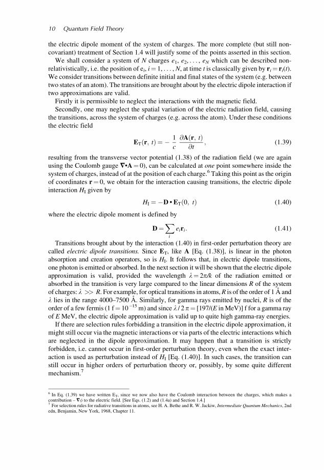
the electric dipole moment of the system of charges. The more complete (but still non-

covariant) treatment of Section 1.4 will justify some of the points asserted in this section.

We shall consider a system of N charges e1, e2, . . . , eN which can be described non-

relativistically, i.e. the position of ei, i¼ 1, . . . , N, at time t is classically given by ri¼ ri(t).

We consider transitions between definite initial and final states of the system (e.g. between

two states of an atom). The transitions are brought about by the electric dipole interaction if

two approximations are valid.

Firstly it is permissible to neglect the interactions with the magnetic field.

Secondly, one may neglect the spatial variation of the electric radiation field, causing

the transitions, across the system of charges (e.g. across the atom). Under these conditions

the electric field

ET r; tð Þ ¼ � 1

c

@A r; tð Þ@t

; (1:39)

resulting from the transverse vector potential (1.38) of the radiation field (we are again

using the Coulomb gauge =•A¼ 0), can be calculated at one point somewhere inside the

system of charges, instead of at the position of each charge.6 Taking this point as the origin

of coordinates r¼ 0, we obtain for the interaction causing transitions, the electric dipole

interaction HI given by

HI ¼ �D • ET 0; tð Þ (1:40)

where the electric dipole moment is defined by

D¼X

i

eiri: (1:41)

Transitions brought about by the interaction (1.40) in first-order perturbation theory are

called electric dipole transitions. Since ET, like A [Eq. (1.38)], is linear in the photon

absorption and creation operators, so is HI. It follows that, in electric dipole transitions,

one photon is emitted or absorbed. In the next section it will be shown that the electric dipole

approximation is valid, provided the wavelength l¼ 2p/k of the radiation emitted or

absorbed in the transition is very large compared to the linear dimensions R of the system

of charges: l >> R. For example, for optical transitions in atoms, R is of the order of 1 A and

l lies in the range 4000–7500 A. Similarly, for gamma rays emitted by nuclei, R is of the

order of a few fermis (1 f¼ 10 –15 m) and since l / 2p¼ [197/(E in MeV)] f for a gamma ray

of E MeV, the electric dipole approximation is valid up to quite high gamma-ray energies.

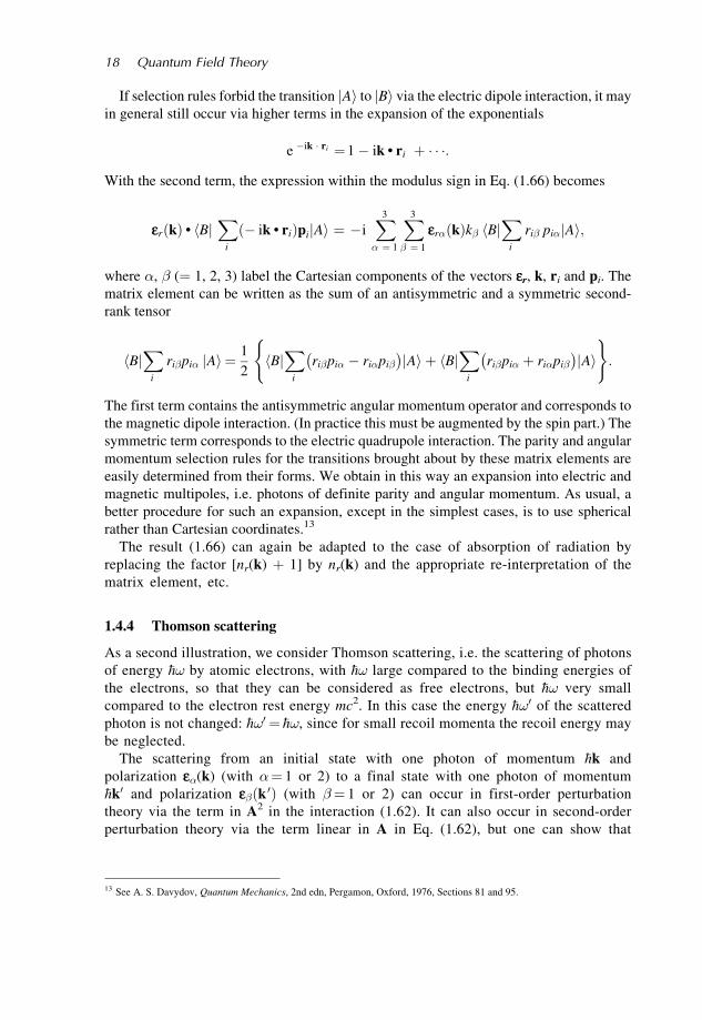
If there are selection rules forbidding a transition in the electric dipole approximation, it

might still occur via the magnetic interactions or via parts of the electric interactions which

are neglected in the dipole approximation. It may happen that a transition is strictly

forbidden, i.e. cannot occur in first-order perturbation theory, even when the exact inter-

action is used as perturbation instead of HI [Eq. (1.40)]. In such cases, the transition can

still occur in higher orders of perturbation theory or, possibly, by some quite different

mechanism.7

6 In Eq. (1.39) we have written ET, since we now also have the Coulomb interaction between the charges, which makes acontribution – =� to the electric field. [See Eqs. (1.2) and (1.4a) and Section 1.4.]7 For selection rules for radiative transitions in atoms, see H. A. Bethe and R. W. Jackiw, Intermediate Quantum Mechanics, 2ndedn, Benjamin, New York, 1968, Chapter 11.


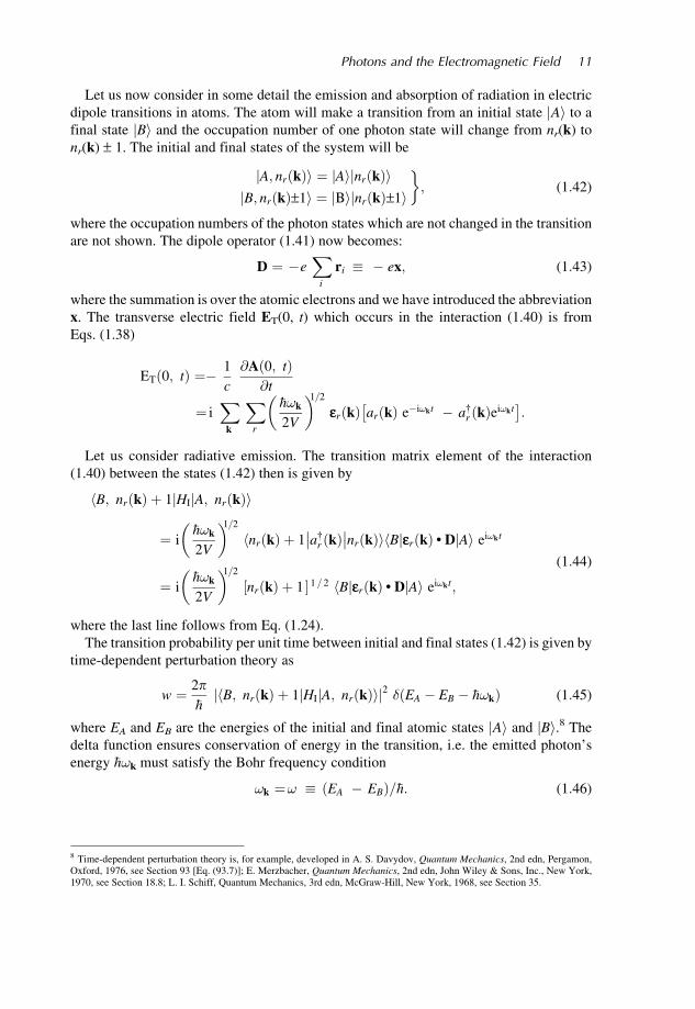
Let us now consider in some detail the emission and absorption of radiation in electric

dipole transitions in atoms. The atom will make a transition from an initial state Aj i to a

final state Bj i and the occupation number of one photon state will change from nr(k) to

nr(k) – 1. The initial and final states of the system will be

jA; nr kð Þi ¼ jAijnr kð ÞijB; nr kð Þ–1i ¼ jBijnr kð Þ–1i

�; (1:42)

where the occupation numbers of the photon states which are not changed in the transition

are not shown. The dipole operator (1.41) now becomes:

D ¼ �eX

i

ri � � ex; (1:43)

where the summation is over the atomic electrons and we have introduced the abbreviation

x. The transverse electric field ET(0, t) which occurs in the interaction (1.40) is from

Eqs. (1.38)

ET 0; tð Þ ¼� 1

c

@A 0; tð Þ@t

¼ iX

k

Xr

�h!k

2V

� �1=2er kð Þ ar kð Þ e�i!kt � a†

r kð Þei!kt� �

:

Let us consider radiative emission. The transition matrix element of the interaction

(1.40) between the states (1.42) then is given by

B; nr kð Þ þ 1 HIj jA; nr kð Þh i

¼ i�h!k

2V

� �1=2hnr kð Þ þ 1 a†

r kð Þ nr kð ÞihB er kð Þ • Dj jAi ei!kt

¼ i�h!k

2V

� �1=2nr kð Þ þ 1½ �1=2 hB er kð Þ • Dj jAi ei!kt;

(1:44)

where the last line follows from Eq. (1.24).

The transition probability per unit time between initial and final states (1.42) is given by

time-dependent perturbation theory as

w ¼ 2p�hhB; nr kð Þ þ 1 HIj jA; nr kð Þij j2 � EA � EB � �h!kð Þ (1:45)

where EA and EB are the energies of the initial and final atomic states Aj i and Bj i.8 The

delta function ensures conservation of energy in the transition, i.e. the emitted photon’s

energy �h!k must satisfy the Bohr frequency condition

!k ¼! � EA � EBð Þ=�h: (1:46)

8 Time-dependent perturbation theory is, for example, developed in A. S. Davydov, Quantum Mechanics, 2nd edn, Pergamon,Oxford, 1976, see Section 93 [Eq. (93.7)]; E. Merzbacher, Quantum Mechanics, 2nd edn, John Wiley & Sons, Inc., New York,1970, see Section 18.8; L. I. Schiff, Quantum Mechanics, 3rd edn, McGraw-Hill, New York, 1968, see Section 35.


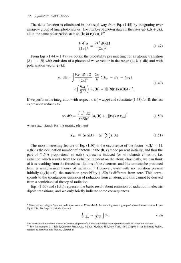
The delta function is eliminated in the usual way from Eq. (1.45) by integrating over

a narrow group of final photon states. The number of photon states in the interval (k, kþ dk),

all in the same polarization state (e1(k) or e2(k)), is9

V d3 k

2pð Þ3¼ Vk2 dk dO

2pð Þ3: (1:47)

From Eqs. (1.44)–(1.47) we obtain the probability per unit time for an atomic transition

Aj i ! Bj i with emission of a photon of wave vector in the range (k, k þ dk) and with

polarization vector er(k):

wr dO ¼ð

Vk2 dk dO

2pð Þ32p�h� EA � EB � �h!kð Þ

�h!k

2 V

� �nr kð Þ þ 1½ � hB er kð Þ•Dj jAij j2:

(1:49)

If we perform the integration with respect to k (¼!k/c) and substitute (1.43) for D, the last

expression reduces to

wr dO ¼ e2!3 dO8p2�hc3

nr kð Þ þ 1½ � er kð Þ•xBAj j2 (1:50)

where xBA stands for the matrix element

xBA � hBjxjAi ¼hBjX

i

rijAi: (1:51)

The most interesting feature of Eq. (1.50) is the occurrence of the factor [nr(k) þ 1].

nr(k) is the occupation number of photons in the (k, r) mode present initially, and thus the

part of (1.50) proportional to nr(k) represents induced (or stimulated) emission, i.e.

radiation which results from the radiation incident on the atom; classically, we can think

of it as resulting from the forced oscillations of the electrons, and this term can be produced

from a semiclassical theory of radiation.10 However, even with no radiation present

initially (nr(k)¼ 0), the transition probability (1.50) is different from zero. This corre-

sponds to the spontaneous emission of radiation from an atom, and this cannot be derived

from a semiclassical theory of radiation.

Eqs. (1.50) and (1.51) represent the basic result about emission of radiation in electric

dipole transitions, and we only briefly indicate some consequences.

9 Since we are using a finite normalization volume V, we should be summing over a group of allowed wave vectors k [seeEq. (1.13)]. For large V (strictly V!1)

1

V

Xk

! 1

2pð Þ3

ðd3k: (1:48)

The normalization volume V must of course drop out of all physically significant quantities such as transition rates etc.10 See, for example, L. I. Schiff, Quantum Mechanics, 3rd edn, McGraw-Hill, New York, 1968, Chapter 11, or Bethe and Jackiw,referred to earlier in this section, Chapter 10.


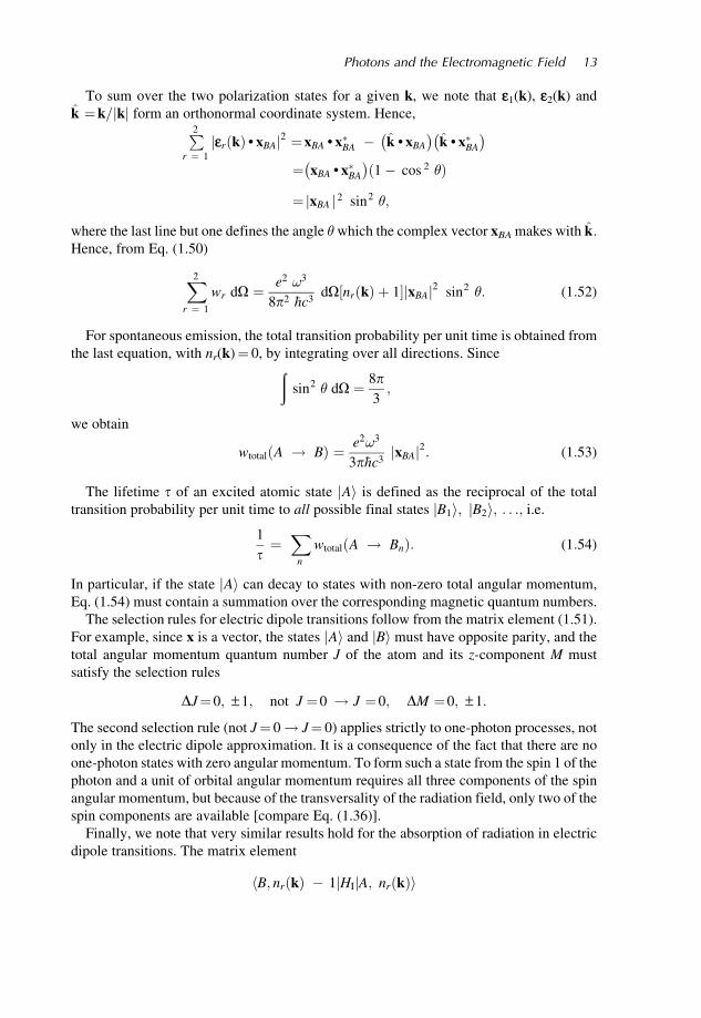
To sum over the two polarization states for a given k, we note that e1(k), e2(k) and

k ¼k=jkj form an orthonormal coordinate system. Hence,P2r ¼ 1

er kð Þ • xBAj j2 ¼xBA • x�BA � k • xBA

� �k • x�BA

� �¼ xBA • x�BA

� �1� cos 2 �ð Þ

¼ xBAj j 2 sin2 �;

where the last line but one defines the angle �which the complex vector xBA makes with k.

Hence, from Eq. (1.50)

X2

r ¼ 1

wr dO ¼ e2 !3

8p2 �hc3dO nr kð Þ þ 1½ � xBAj j2 sin2 �: (1:52)

For spontaneous emission, the total transition probability per unit time is obtained from

the last equation, with nr(k)¼ 0, by integrating over all directions. Sinceðsin2 � dO ¼ 8p

3;

we obtain

wtotal A ! Bð Þ ¼ e2!3

3p�hc3xBAj j2: (1:53)

The lifetime t of an excited atomic state Aj i is defined as the reciprocal of the total

transition probability per unit time to all possible final states B1i; B2i; . . .;jj i.e.

1

t¼X

n

wtotal A ! Bnð Þ: (1:54)

In particular, if the state Aj i can decay to states with non-zero total angular momentum,

Eq. (1.54) must contain a summation over the corresponding magnetic quantum numbers.

The selection rules for electric dipole transitions follow from the matrix element (1.51).

For example, since x is a vector, the states Aj i and Bj i must have opposite parity, and the

total angular momentum quantum number J of the atom and its z-component M must

satisfy the selection rules

DJ¼0; – 1; not J ¼0 ! J ¼0; DM ¼0; – 1:

The second selection rule (not J¼ 0! J¼ 0) applies strictly to one-photon processes, not

only in the electric dipole approximation. It is a consequence of the fact that there are no

one-photon states with zero angular momentum. To form such a state from the spin 1 of the

photon and a unit of orbital angular momentum requires all three components of the spin

angular momentum, but because of the transversality of the radiation field, only two of the

spin components are available [compare Eq. (1.36)].

Finally, we note that very similar results hold for the absorption of radiation in electric

dipole transitions. The matrix element

hB; nr kð Þ � 1 HIj jA; nr kð Þi


corresponding to Eq. (1.44) now involves the factor [nr(k)]1/2 instead of [nr(k)þ 1]1/2. Our

final result for emission, Eq. (1.50), also holds for absorption, with [nr(k)þ 1] replaced by

[nr(k)], dO being the solid angle defining the incident radiation, and the matrix element

xBA, Eq. (1.51), representing a transition from an atomic state Aj i with energy EA to a state

Bj i with energy EB > EA. Correspondingly, the frequency ! is defined by �h!¼EB – EA

instead of Eq. (1.46).

1.4 The Electromagnetic Field in the Presence of Charges

After the special case of the electric dipole interaction, we now want to consider the

general interaction of moving charges and an electromagnetic field. As this problem will

later be treated in a relativistically covariant way, we shall not give a rigorous complete

derivation, but rather stress the physical interpretation. As in the last section, the motion of

the charges will again be described non-relativistically. In Section 1.4.1 we shall deal with

the Hamiltonian formulation of the classical theory. This will enable us very easily to go

over to the quantized theory in Section 1.4.2. In Sections 1.4.3 and 1.4.4 we shall illustrate

the application of the theory for radiative transitions and Thomson scattering.

1.4.1 Classical electrodynamics

We would expect the Hamiltonian of a system of moving charges, such as an atom, in an

electromagnetic field to consist of three parts: a part referring to matter (i.e. the charges), a

part referring to the electromagnetic field and a part describing the interaction between

matter and field.

For a system of point masses mi, i¼ 1, . . . , N, with charges ei and position coordinates ri,

the Hamiltonian is

Hm ¼X

i

p2i

2mi

þ HC (1:55a)

where HC is the Coulomb interaction

HC �1

2

Xi; j

i 6¼ jð Þ

eiej

4p ri � rj

(1:55b)

and pi¼mi dri/dt is the kinetic momentum of the ith particle. This is the usual Hamiltonian

of atomic physics, for example.

The electromagnetic field in interaction with charges is described by Maxwell’s equa-

tions [Eqs. (1.1)]. We continue to use the Coulomb gauge, = • A¼ 0, so that the electric

field (1.2) decomposes into transverse and longitudinal fields

E ¼ET þ EL;

where

ET ¼ �1

c

@A

@t; EL ¼ � =�:


(A longitudinal field is defined by the condition = ^ EL¼ 0.) The magnetic field is given

by B¼= ^ A.

The total energy of the electromagnetic field

1

2

ðE2 þ B2� �

d3x

can be written

1

2

ðE2

T þ B2� �

d3x þ 1

2

ðE2

L d3x:

The last integral can be transformed, using Poisson’s equation =2 � ¼ � �; into

1

2

ðE2

L d3x ¼ 1

2

ð� x; tð Þ� x

0; t

� �4p x � x

0j j d3x d3x0: (1:56)

Thus the energy associated with the longitudinal field is the energy of the instantaneous

electrostatic interaction between the charges. With

� x; tð Þ ¼X

i

ei � x � ri tð Þð Þ

Eq. (1.56) reduces to

1

2

ðE2

L d3x¼ 1

2

Xi; j

eiej

4p ri � rj

¼ 1

2

Xi; j

i 6¼ j

eiej

4p ri � rj

� HC;

(1:57)

where, in the last line, we have dropped the infinite self-energy which occurs for point

charges. The term HC has already been included in the Hamiltonian Hm, Eqs. (1.55), so we

must take as additional energy of the electromagnetic field that of the transverse radiation

field

Hrad ¼1

2

ðE2

T þ B2� �

d3x: (1:58)

Eqs. (1.55) allow for the instantaneous Coulomb interaction of charges. To allow for the

interaction of moving charges with an electromagnetic field, one must replace the matter-

Hamiltonian (1.55a) by

H0

m ¼X

i

1

2mi

pi �ei

cAi

� �2

þ HC (1:59)

where Ai,¼A(ri, t) denotes the vector potential at the position ri of the charge ei at time t.

In Eq. (1.59) pi is the momentum coordinate canonically conjugate to the position

coordinate ri, in the sense of Lagrangian mechanics, and it is related to the velocity

vi¼ dri/dt of the ith particle by

pi ¼mivi þei

cAi:


It is only for A¼ 0 that this conjugate momentum reduces to the kinetic momentum mivi.

The justification for the form (1.59) for H0m is that it gives the correct equations of motion

for the charges (see Problem 1.2):

mi

dvi

dt¼ ei Ei þ

vi

c^ Bi

h i; (1:60)

where Ei and Bi are the electric and magnetic fields at the instantaneous position of the ith

charge.11

We can regroup the terms in Eq. (1.59) as

H0

m ¼ Hm þ HI (1:61)

where HI, the interaction Hamiltonian of matter and field, is given by

HI ¼X

i

� ei

2micpi • Ai þ Ai • pið Þ þ e2

i

2mic2A2

i

�

¼X

i

� ei

micAi • pi þ

e2i

2mic2A2

i

�:

(1:62)

In the quantum theory pi, the momentum canonically conjugate to ri, will become the operator

�i�h=i. Nevertheless, the replacement of pi • Ai by Ai • pi in the second line of Eq. (1.62) is

justified by our gauge condition =i • Ai ¼0. Eq. (1.62) represents the general interaction of

moving charges in an electromagnetic field (apart from HC). It does not include the interaction

of the magnetic moments, such as that due to the spin of the electron, with magnetic fields.

Combining the above results (1.55), (1.58), (1.59) and (1.62), we obtain for the complete

Hamiltonian

H ¼H0

m þ Hrad ¼Hm þ Hrad þ HI: (1:63)

Just as this Hamiltonian leads to the correct equations of motion (1.60) for charges, so it

also leads to the correct field equations (1.4), with =•A¼0, for the potentials.12

1.4.2 Quantum electrodynamics

The quantization of the system described by the Hamiltonian (1.63) is carried out by

subjecting the particles’ coordinates ri and canonically conjugate momenta pi to the usual

commutation relations (e.g. in the coordinate representation pi ! � i�h=i), and quantiz-

ing the radiation field, as in Section 1.2.3. The longitudinal electric field EL does not

provide any additional degrees of freedom, being completely determined via the first

Maxwell equation = • EL ¼� by the charges.

The interaction HI in Eq, (1.63) is usually treated as a perturbation which causes

transitions between the states of the non-interacting Hamiltonian

H0 ¼Hm þ Hrad: (1:64)

11 For the Lagrangian and Hamiltonian formulations of mechanics which are here used see, for example, H. Goldstein, ClassicalMechanics, 2nd edn, Addison-Wesley, Reading, Mass., 1980, in particular pp. 21–23 and 346.12 See W. Heitler, The Quantum Theory of Radiation, 3rd edn, Clarendon Press, Oxford, 1954, pp. 48–50.


The eigenstates of H0 are again of the form

A; . . . nr kð Þ . . .j i ¼ Aj i . . . nr kð Þ . . .j i;

with Aj i and . . . nr kð Þ . . .j i eigenstates of Hm and Hrad.

Compared with the electric dipole interaction (1.40), the interaction (1.62) differs in that

it contains a term quadratic in the vector potential. This results in two-photon processes in

first-order perturbation theory (i.e. emission or absorption of two photons or scattering). In

addition, the first term in (1.62) contains magnetic interactions and higher-order effects

due to the spatial variation of A(x, t), which are absent from the electric dipole interaction

(1.40). These aspects are illustrated in the applications to radiative transitions and

Thomson scattering which follow.

1.4.3 Radiative transitions in atoms

We consider transitions between two states of an atom with emission or absorption of one

photon. This problem was treated in Section 1.3 in the electric dipole approximation, but

now we shall use the interaction (1.62).

We shall consider the emission process between the initial and final states (1.42). Using

the expansion (1.38) of the vector potential, we obtain the matrix element for this transition

[which results from the term linear in A in Eq. (1.62)]

hB; nr kð Þ þ 1 HIj jA; nr kð Þi

¼� e

m

�h

2V!k

� �1=2

nr kð Þ þ 1½ �1=2 hBjer kð Þ •X

i

e�ik • ri pijAi ei!kt:(1:65)

Using this matrix element, one calculates the transition probability per unit time as in

Section 1.3. Instead of Eqs. (1.50) and (1.51), one obtains:

wr dO ¼ e2! dO8p2m2�hc3

nr kð Þ þ 1½ � er kð Þ•hBjX

i

e� ik • ri pi jAi

2

: (1:66)

These results go over into the electric dipole approximation if in the matrix elements in

Eqs. (1.65) and (1.66) we can approximate the exponential functions by unity:

e� ik • ri »1: (1:67)

This is justified provided the wavelength l¼ 2p / k of the radiation emitted in the transition is

very large compared to the linear dimensions R of the system of charges (in our case, of the

atom): l>> R. The atomic wavefunctions jAi and jBi restrict the effective values of ri to ri9R,

so that k • ri 9 kR << 1. We saw in Section 1.3 that this inequality is generously satisfied

for optical atomic transitions. From the equation of motion i�h _ri ¼ ri; H½ � and Eq. (1.46)

B pij jAh i ¼m B _rij jAh i ¼ � im! B rij jAh i:

Hence, in the approximation (1.67), Eqs. (1.65) and (1.66) reduce to the electric dipole

form, Eqs. (1.44) and (1.50).


If selection rules forbid the transition Aj i to Bj i via the electric dipole interaction, it may

in general still occur via higher terms in the expansion of the exponentials

e �ik � ri ¼1� ik • ri þ � � �:

With the second term, the expression within the modulus sign in Eq. (1.66) becomes

er kð Þ • Bh jX

i

� ik • rið Þpi Aj i ¼ �iX3

� ¼ 1

X3

� ¼ 1

er� kð Þk� Bh jX

i

ri� pi� Aj i;

where �, � (¼ 1, 2, 3) label the Cartesian components of the vectors er, k, ri and pi. The

matrix element can be written as the sum of an antisymmetric and a symmetric second-

rank tensor

Bh jX

i

ri�pi� Aj i ¼ 1

2Bh jX

i

ri�pi� � ri�pi�

� �Aj i þ Bh j

Xi

ri�pi� þ ri�pi�

� �Aj i

( ):

The first term contains the antisymmetric angular momentum operator and corresponds to

the magnetic dipole interaction. (In practice this must be augmented by the spin part.) The

symmetric term corresponds to the electric quadrupole interaction. The parity and angular

momentum selection rules for the transitions brought about by these matrix elements are

easily determined from their forms. We obtain in this way an expansion into electric and

magnetic multipoles, i.e. photons of definite parity and angular momentum. As usual, a

better procedure for such an expansion, except in the simplest cases, is to use spherical

rather than Cartesian coordinates.13

The result (1.66) can again be adapted to the case of absorption of radiation by

replacing the factor [nr(k) þ 1] by nr(k) and the appropriate re-interpretation of the

matrix element, etc.

1.4.4 Thomson scattering

As a second illustration, we consider Thomson scattering, i.e. the scattering of photons

of energy �h! by atomic electrons, with �h! large compared to the binding energies of

the electrons, so that they can be considered as free electrons, but �h! very small

compared to the electron rest energy mc2. In this case the energy �h!0 of the scattered

photon is not changed: �h!0 ¼ �h!, since for small recoil momenta the recoil energy may

be neglected.

The scattering from an initial state with one photon of momentum �hk and

polarization e�(k) (with �¼ 1 or 2) to a final state with one photon of momentum

�hk0 and polarization e� k 0ð Þ (with �¼ 1 or 2) can occur in first-order perturbation

theory via the term in A2 in the interaction (1.62). It can also occur in second-order

perturbation theory via the term linear in A in Eq. (1.62), but one can show that

13 See A. S. Davydov, Quantum Mechanics, 2nd edn, Pergamon, Oxford, 1976, Sections 81 and 95.


under our conditions the contribution of the second-order process is negligible.14 The

operator A2(0, t) can, from Eq. (1.38), be written

A2 0; tð Þ ¼Xk1k2

Xr; s

�hc2

2V !1 !2ð Þ1=2er k1ð Þ • es k2ð Þð Þ

ar k1ð Þe�i!1t þ a†r k1ð Þ eþ i!1t

� �as k2ð Þe�i!2t þ a†

s k2ð Þ eþi!2t� �

;

(1:68)

where !r� c|kr|, r¼ 1, 2. This operator can bring about the transition from the initial state

k; �j i to the final state k 0; �j i (we use a somewhat simplified, but unambiguous, notation)

in two ways: either of the factors in square parentheses can act to absorb the initial photon,

and the other factor then creates the final photon. One then obtains the matrix element for

this transition from Eq. (1.62)

hk 0 ; �j e2

2mc2A2 0; tð Þ jk; �i ¼ e2�h

2mV !! 0ð Þ1=2e� kð Þ • e�ðk

0 Þ ei !0 � !ð Þt

where ! ¼ c kj j and. ! 0 ¼ c k 0j j: The transition probability per unit time for a photon,

initially in the state jk; �i, to be scattered into an element of solid angle dW in the

direction k0, and with polarization e� k 0ð Þ, is given by

w� ! � k0� �

dO ¼ 2p�h

ðVk

02 dk0dO

2pð Þ3�ð�h! 0 � �h!Þ

e2�h

2mV

� �21

!! 0

� �e� kð Þ • e�ðk

0 Þ� � 2

¼ c

V

e2

4pmc2

� �2

e� kð Þ • e�ðk0 Þ

h i 2

dO

where k 0j j¼ kj j. Dividing this transition probability per unit time by the incident photon

flux (c/V), one obtains the corresponding differential cross-section

�� ! � ðk0 Þ dO ¼ r2

0 e� kð Þ • e�ðk0 Þ

h i2

dO; (1:69)

where the classical electron radius has been introduced by

r0 ¼e2

4pmc2¼2:818 fm: (1:70)

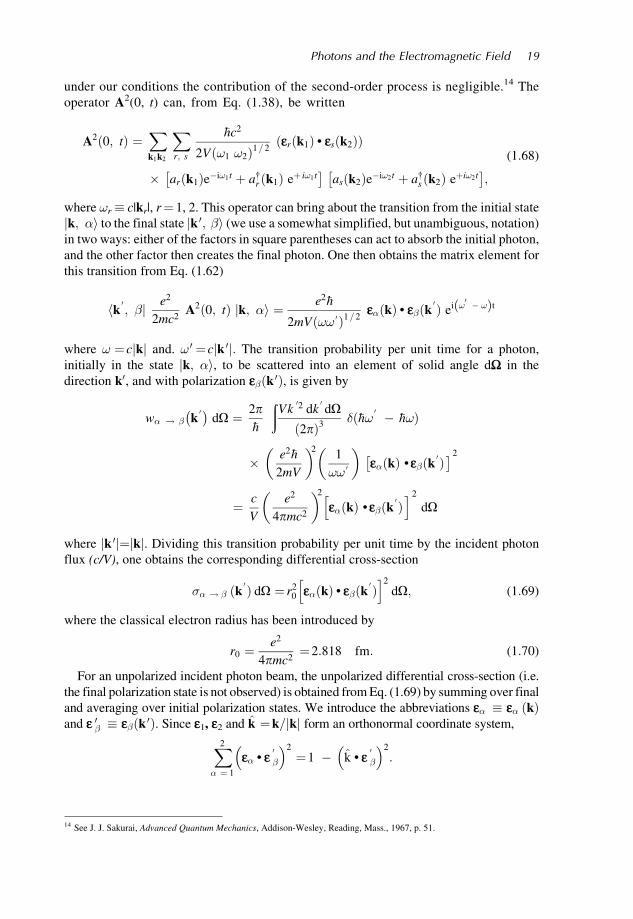
For an unpolarized incident photon beam, the unpolarized differential cross-section (i.e.

the final polarization state is not observed) is obtained from Eq. (1.69) by summing over final

and averaging over initial polarization states. We introduce the abbreviations e� � e� kð Þand e 0� � e� k 0ð Þ. Since e1, e2 and k ¼k= kj j form an orthonormal coordinate system,

X2

� ¼ 1

e� • e0

�

� �2

¼1 � k • e0

�

� �2

:

14 See J. J. Sakurai, Advanced Quantum Mechanics, Addison-Wesley, Reading, Mass., 1967, p. 51.


Similarly

X2

� ¼ 1

k • e0

�

� �2

¼ 1 � k • k0

� �2

¼ sin2 �

where � is the angle between the directions k and k0 of the incident and scattered photons,

i.e. the angle of scattering. From the last two equations

1

2

X2

� ¼ 1

X2

� ¼ 1

e� • e0

�

� �2

¼ 1

22 � sin2 ��

¼ 1

21þ cos2 ��

(1:71)

and hence the unpolarized differential cross-section for scattering through an angle � is

from Eq. (1.69) given as

� �ð Þ dO ¼ 1

2r2

0 1 þ cos2 ��

dO: (1:69a)

Integrating over angles, we obtain the total cross-section for Thomson scattering

�total ¼8p3

r20 ¼6:65 10�25 cm2: (1:72)

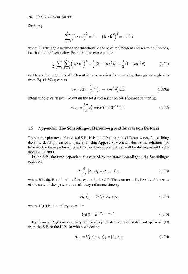
1.5 Appendix: The Schrodinger, Heisenberg and Interaction Pictures

These three pictures (abbreviated S.P., H.P. and I.P.) are three different ways of describing

the time development of a system. In this Appendix, we shall derive the relationships

between the three pictures. Quantities in these three pictures will be distinguished by the

labels S, H and I.

In the S.P., the time-dependence is carried by the states according to the Schrodinger

equation

i�hd

dtA; tiS ¼H A; tiS;j (1:73)

where H is the Hamiltonian of the system in the S.P. This can formally be solved in terms

of the state of the system at an arbitrary reference time t0

A; tj iS ¼US tð Þ jA; t0iS (1:74)

where US(t) is the unitary operator:

US tð Þ ¼ e�iH t � t0ð Þ =�h: (1:75)

By means of US(t) we can carry out a unitary transformation of states and operators (O)

from the S.P. to the H.P., in which we define

Aj iH ¼U†S tð Þ A; tj iS ¼ A; t0j iS (1:76)


and

OH tð Þ ¼U†S tð ÞOS US tð Þ: (1:77)

At t¼ t0, states and operators in the two pictures are the same. We see from Eq. (1.76)

that in the H.P. state, vectors are constant in time; the time-dependence is carried by the

Heisenberg operators. From Eq. (1.77)

HH ¼HS � H: (1:78)

Since the transformation from the S.P. to the H.P. is unitary, it ensures the invariance of

matrix elements and commutation relations:

ShB; tjOS A; tiS ¼ HhB; t OH tð Þ A; tiH;

(1:79)

and if O and P are two operators for which [OS, PS]¼ const., then [OH(t), PH(t)] equals the

same constant.

Differentation of Eq. (1.77) gives the Heisenberg equation of motion

i�hd

dtOH tð Þ ¼ OH tð Þ; H

� �: (1:80)

For an operator which is time dependent in the S.P. (corresponding to a quantity which

classically has an explicit time dependence), Eq. (1.80) is augmented to

i�hd

dtOH tð Þ ¼ i�h

@

@tOH tð Þ þ OH tð Þ; H

� �: (1:81)

We shall not be considering such operators.

The I.P. arises if the Hamiltonian is split into two parts

H ¼H0 þ HI: (1:82)

In quantum field theory, HI will describe the interaction between two fields, themselves

described by H0. [Note that the suffix I on HI stands for ‘interaction’. It does not label a

picture. Eq. (1.82) holds in any picture.] The I.P. is related to the S.P. by the unitary

transformation

U0 tð Þ ¼ e�iH0 t � t0ð Þ= �h (1:83)

i.e.

A; tj iI ¼U†0 tð Þ A; tj iS (1:84)

and

OI tð Þ ¼U†0 tð ÞOS U0 tð Þ: (1:85)

Thus the relation between I.P. and S.P. is similar to that between H.P. and S.P., but with the

unitary transformation U0 involving the non-interacting Hamiltonian H0, instead of U

involving the total Hamiltonian H. From Eq. (1.85):

HI0 ¼HS

0 � H0: (1:86)


Differentiating Eq. (1.85) gives the differential equation of motion of operators in the I.P.:

i�hd

dtOI tð Þ ¼ OI tð Þ; H0

� �: (1:87)

Substituting Eq. (1.84) into the Schrodinger equation (1.73), one obtains the equation of

motion of state vectors in the I.P.

i�hd

dtA; tiI ¼HI

I tð Þ A; tiI (1:88)

where

HII tð Þ ¼ eiH0 t � t0ð Þ=�h HS

I e�iH0 t � t0ð Þ= �h: (1:89)

Finally, from the above relations, one easily shows that the I.P. and H.P. are related by

OI tð Þ ¼U tð ÞOH tð ÞU† tð Þ (1:90)

A; tj iI ¼U tð Þ Aj iH (1:91)

where the unitary operator U(t) is defined by

U tð Þ ¼ eiH0 t � t0ð Þ= �h e�iH t � t0ð Þ=�h: (1:92)

The time development of the I.P. states follows from Eq. (1.91). From this equation

A; t1j iI ¼U t1ð Þ Aj iH ¼U t1ð ÞU† t2ð Þ A; t2j iI:

Hence

A; t1j iI ¼U t1; t2ð Þ A; t2j iI (1:93)

where the unitary operator U(t1, t2), defined by

U t1; t2ð Þ ¼U t1ð ÞU† t2ð Þ; (1:94)

satisfies the relations

U† t1; t2ð Þ ¼U t2; t1ð Þ (1:95a)

U t1; t2ð ÞU t2; t3ð Þ ¼U t1; t3ð Þ: (1:95b)

Problems

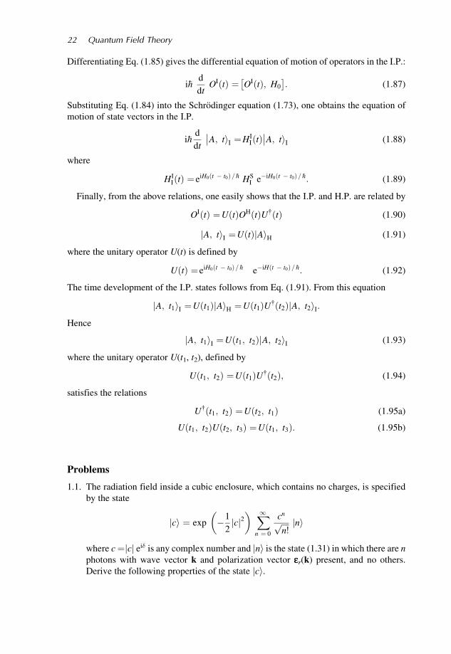
1.1. The radiation field inside a cubic enclosure, which contains no charges, is specified

by the state

cj i ¼ exp �1

2cj j2

� � X1n ¼ 0

cnffiffiffiffin!p nj i

where c¼ cj j ei� is any complex number and jni is the state (1.31) in which there are n

photons with wave vector k and polarization vector er(k) present, and no others.

Derive the following properties of the state cj i.


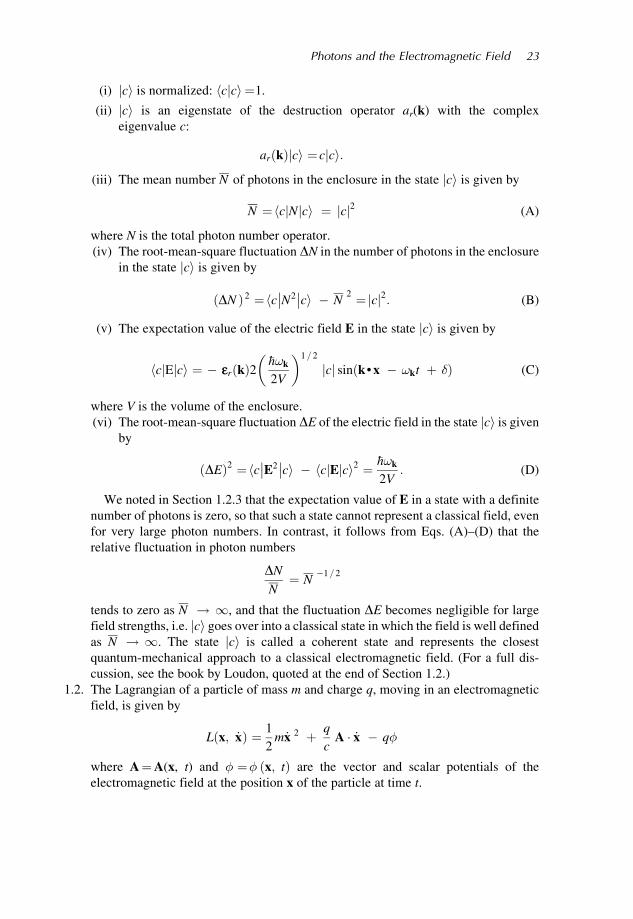
(i) cj i is normalized: cjch i ¼1.

(ii) cj i is an eigenstate of the destruction operator ar(k) with the complex

eigenvalue c:

ar kð Þ cj i ¼ c cj i:

(iii) The mean number N of photons in the enclosure in the state jci is given by

N ¼hcjNjci ¼ jcj2 (A)

where N is the total photon number operator.

(iv) The root-mean-square fluctuation DN in the number of photons in the enclosure

in the state cj i is given by

ðDN Þ2 ¼hc N2 ci � N

2 ¼jcj2: (B)

(v) The expectation value of the electric field E in the state cj i is given by

hcjEjci ¼ � er kð Þ2 �h!k

2V

� �1=2

jcj sin k• x � !kt þ �ð Þ (C)

where V is the volume of the enclosure.

(vi) The root-mean-square fluctuation DE of the electric field in the state cj i is given

by

DEð Þ2 ¼hc E2 ci � hcjEjci2 ¼ �h!k

2V: (D)

We noted in Section 1.2.3 that the expectation value of E in a state with a definite

number of photons is zero, so that such a state cannot represent a classical field, even

for very large photon numbers. In contrast, it follows from Eqs. (A)–(D) that the

relative fluctuation in photon numbers

DN

N¼ N

�1=2

tends to zero as N ! 1, and that the fluctuation DE becomes negligible for large

field strengths, i.e. jci goes over into a classical state in which the field is well defined

as N ! 1. The state cj i is called a coherent state and represents the closest

quantum-mechanical approach to a classical electromagnetic field. (For a full dis-

cussion, see the book by Loudon, quoted at the end of Section 1.2.)

1.2. The Lagrangian of a particle of mass m and charge q, moving in an electromagnetic

field, is given by

L x; _xð Þ ¼ 1

2m _x 2 þ q

cA � _x � q�

where A¼A(x, t) and � ¼� x; tð Þ are the vector and scalar potentials of the

electromagnetic field at the position x of the particle at time t.


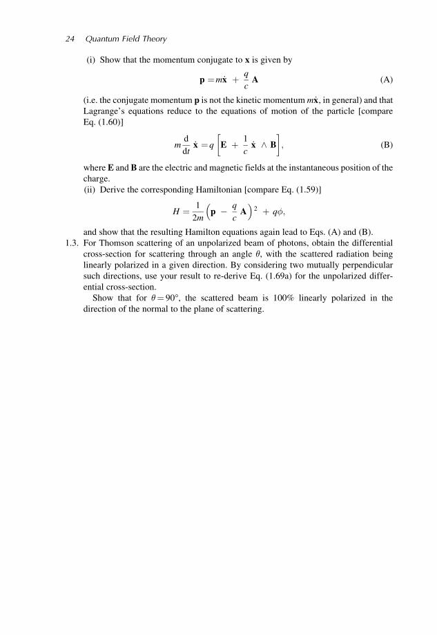
(i) Show that the momentum conjugate to x is given by

p ¼m _x þ q

cA (A)

(i.e. the conjugate momentum p is not the kinetic momentum m _x, in general) and that

Lagrange’s equations reduce to the equations of motion of the particle [compare

Eq. (1.60)]

md

dt_x ¼q E þ 1

c_x ^ B

� �; (B)

where E and B are the electric and magnetic fields at the instantaneous position of the

charge.

(ii) Derive the corresponding Hamiltonian [compare Eq. (1.59)]

H ¼ 1

2mp � q

cA

� �2 þ q�;

and show that the resulting Hamilton equations again lead to Eqs. (A) and (B).

1.3. For Thomson scattering of an unpolarized beam of photons, obtain the differential

cross-section for scattering through an angle �, with the scattered radiation being

linearly polarized in a given direction. By considering two mutually perpendicular

such directions, use your result to re-derive Eq. (1.69a) for the unpolarized differ-

ential cross-section.

Show that for �¼ 90�, the scattered beam is 100% linearly polarized in the

direction of the normal to the plane of scattering.


Documents

PhotonsandtheElectromagneticField COPYRIGHTED MATERIAL · The foundations of a systematic quantum theory of fields were laid by Dirac in 1927 in his famous paper on ‘The Quantum