Embed Size (px)
Citation preview
SCUOLA NORMALE SUPERIORE DI PISA
Perfezionamento in Matematica
XVIII ciclo, anni 2003-2005
PhD Thesis
Federica Dragoni
CARNOT-CARATHEODORY
METRICS AND VISCOSITY
SOLUTIONS
Advisor: Prof. Italo Capuzzo Dolcetta

Contents
Introduction. 5
1 Sub-Riemannian geometries. 11
1.1 Basic definitions and main properties. . . . . . . . . . . . . . . 11
1.1.1 Historical introduction and Dido’s problem. . . . . . . 11
1.1.2 Some new development: the visual cortex. . . . . . . . 15
1.1.3 Riemannian metrics. . . . . . . . . . . . . . . . . . . . 17
1.1.4 Carnot-Caratheodory metrics and the Hormander con-
dition. . . . . . . . . . . . . . . . . . . . . . . . . . . . 21
1.1.5 Notions equivalent to the Carnot-Caratheodory distance. 27
1.1.6 Chow’s Theorem. . . . . . . . . . . . . . . . . . . . . . 33
1.1.7 Relationship between the Carnot-Caratheodory dis-
tance and the Euclidean distance. . . . . . . . . . . . . 36
1.1.8 Sub-Riemannian geodesics. . . . . . . . . . . . . . . . . 39
1.1.9 The Grusin plane. . . . . . . . . . . . . . . . . . . . . . 44
1.2 Carnot groups. . . . . . . . . . . . . . . . . . . . . . . . . . . 49
1.2.1 Nilpotent Lie groups. . . . . . . . . . . . . . . . . . . . 49
1.2.2 Calculus on Carnot groups. . . . . . . . . . . . . . . . 53
1.3 The Heisenberg group. . . . . . . . . . . . . . . . . . . . . . . 56
1.3.1 The polarized Heisenberg group. . . . . . . . . . . . . . 57
1.3.2 The canonical Heisenberg group. . . . . . . . . . . . . 60
1.3.3 Equivalence of the two definitions. . . . . . . . . . . . . 64
2 Viscosity solutions and metric Hopf-Lax formula. 71
2.1 An introduction to the theory of viscosity solutions. . . . . . . 71
2.1.1 Viscosity solutions for continuous functions. . . . . . . 73
3
4 Contents.
2.1.2 Discontinuous viscosity solutions. . . . . . . . . . . . . 79
2.2 The generalized eikonal equation. . . . . . . . . . . . . . . . . 87
2.3 The Hopf-Lax function. . . . . . . . . . . . . . . . . . . . . . . 97
2.3.1 Optimal control theory and Hopf-Lax formula. . . . . . 97
2.3.2 Some properties of the Euclidean Hopf-Lax function. . 102
2.4 The metric Hopf-Lax function. . . . . . . . . . . . . . . . . . . 105
2.4.1 Properties of the metric Hopf-Lax function. . . . . . . 106
2.4.2 The Hopf-Lax solution for the Cauchy problem. . . . . 117
2.4.3 Examples and applications. . . . . . . . . . . . . . . . 122
3 Carnot-Caratheodory inf-convolutions. 127
3.1 Definition and basic properties. . . . . . . . . . . . . . . . . . 127
3.2 Inf-convolutions and logarithms of heat kernels. . . . . . . . . 131
3.2.1 The Euclidean approximation and the Large Deviation
Principle. . . . . . . . . . . . . . . . . . . . . . . . . . 132
3.2.2 Applicability of the Large Deviation Principle: the
proof of Varadhan for the Riemannian case. . . . . . . 136
3.3 Carnot-Caratheodory inf-convolutions and ultraparabolic
equations. . . . . . . . . . . . . . . . . . . . . . . . . . . . . . 141
3.3.1 Heat kernels for hypoelliptic operators. . . . . . . . . . 141
3.3.2 Limiting behavior of solutions of subelliptic heat equa-
tions. . . . . . . . . . . . . . . . . . . . . . . . . . . . . 145
A The Legendre-Fenchel transform. 157
Bibliography. 165

Introduction.
Sub-Riemannian geometries have many interesting applications in very dif-
ferent settings, as optimal control theory ([17, 26, 27]), calculus of variations
([2, 4]) or stochastic differential equations ([16]). Many physical phenomena
seem to induce in a natural way an associated sub-Riemannian structure, for
example, one can think of Berry’s phase problem, a swimming microorgan-
ism (studied in [75]), the optimal control in laser-induced population transfer
(see [20]) and the perceptual completion in the visual cortex ([35]). Sub-
Riemannian geometries (known also as Carnot-Caratheodory spaces) arise
whenever there are privileged and prohibited paths. In fact, the main differ-
ence between these geometries and the Riemannian geometries is the need to
move along some prescribed vector fields. A Sub-Riemannian metric is in-
deed a Riemannian metric defined only on a subbundle of the tangent bundle
to the manifold. More precisely, let X = X1, ..., Xm be a family of vector
fields, defined on a n-dimensional manifold M (with in general m ≤ n), a
sub-Riemannian metric is a Riemannian metric⟨,⟩
defined on the fibers of
H := Span(X ) ⊂ TM . A subbundle H is usually called distribution.
For sake of simplicity, from now on we will always assume thatM = Rn. This
in particular implies that the tanget space at any point x is equal to Rn and
the tangent bundle is isomorphic to R2 n. An admissible (or X -horizontal)
curve is any absolutely continuous curve γ : [0, T ] → Rn, such that
γ(t) ∈ Span(X1(γ(t)), ..., Xm(γ(t))), a.e. t ∈ [0, T ].
Since the Riemannian metric⟨,⟩
is defined along the fibers of H, for the
horizontal curves and, only for the horizontal curves, we can introduce a
6 Introduction.
length-functional as follows:
l(γ) =
∫ T
0
⟨γ(t), γ(t)
⟩ 12dt.
A sub-Riemannian (or Carnot-Caratheodory) distance on Rn can be de-
fined, for any x, y ∈ Rn, as
d(x, y) = infl(γ) | γ admissible curve joiningx to y. (1)
It is obvious that, whenever there are not admissible curves joining x to y,
then d(x, y) = +∞. For this purpose the Hormander condition is introduced.
In fact, in Carnot-Caratheodory spaces satisfying the Hormander condition,
it is always possible to join two given points by an admissible curve (Chow’s
Theorem, [17, 75]). Then the associated Carnot-Caratheodory distance is
finite. The Hormander condition (known also as bracket generating condi-
tion) is satisfied if the Lie algebra associated to the distribution H = Span(X )
spans the whole tangent space at any point of the manifold (that in this par-
ticular case is at any point equal to Rn). We recall that the bracket between
two vector fields X and Y is the vector field defined as [X, Y ] = XY − Y X,
acting by derivation on smooth real functions. The Lie algebra L(X ) associ-
ated to X = X1, ..., Xm is the set of all the brackets between elements of
X , so the Hormander condition holds, if and only if,
Span(L(X1(x), ..., Xm(x))
)= TxM = R
n, for any x ∈ Rn.
The first chapter is dedicated to the study of sub-Riemannian geometries
and topological and metric implications of the Hormander condition.
In the second chapter, we are interested in solving some first-order
nonlinear partial differential equations (PDEs) related to the Hormander
condition. Therefore we will introduce the theory of viscosity solutions
for continuous and discontinuous functions. Later we concentrate on the
two particular nonlinear PDEs: The eikonal equation and an evolution
Hamilton-Jacobi equation.
We first solve the generalized eikonal equation:
H0(x,Du) = 1, (2)
Introduction. 7
with vanishing condition at some fixed point y ∈ Rn and where H0(x, p) is
the geometrical Hamiltonian defined by
H0(x, p) = |σ(x)p|, (3)
with σ(x) Hormander-matrix (i.e. a m × n real-valued matrix with smooth
coefficiente and such that its rows satisfy the Hormander condition).
Later we consider an evolution Hamilton-Jacobi equation of the form:
ut + Φ(H0(x,Du)) = 0 (4)
where Φ is a suitable positive and convex function and H0(x, p) satisfies the
structural assumpiton (2). The main model for the PDE (4) is
ut +1
α|σ(x)Du|α = 0, with α > 1. (5)
We solve both the previous PDEs by using the Hormander condition and
suitable representative formulas. In order to solve the eikonal equation, fixed
the point y ∈ Rn, we define the minimal-time function
d(x, y) = infX(·)∈Fx,y
T (X(·)), (6)
where Fx,y is the set of all the trajectories joining x to y in a time T (X(·))which are solutions of the differential inclusion
X(t) ∈ ∂H0(X(t), 0) = σT (X(t))B1(0),
with B1(0) unit Euclidean ball in Rm centered at the origin.
It is possible to show under very weak assumptions that a minimal-time
distance is a generalized distance (i.e. a distance not always symmetric)
solving a Dynamical Programming Principle:
d(x, y) = infX(·)∈Fx,y
[t+ d(X(t), y)], for any 0 < t < d(x, y).
For our particular Hamiltonian in (3), the minimal-time distance turns out to
be equivalent to the Carnot-Caratheodory distance associated to the matrix
σ(x). By using the Dynamical Programming Principle, we prove that u(x) =
d(x, y) solves in the viscosity sense the corresponding eikonal equations on
8 Introduction.
Rn\y. By a sub-Riemanninan generalization of the Rademacher’s Theorem
(see [75, 77, 80]), the viscosity result implies that the Carnot-Caratheodory
distance is a almost everywhere solution, too (at least in Carnot groups).
To solve the eikonal equation is the key-point in order to solve the Cauchy
problem for Eq. (4) with lower semicontinuous initial data g(x). To get
the existence of a viscosity solution for this class of PDEs, we use a suitable
representative formula: the metric Hopf-Lax formula given by
u(t, x) = infy∈Rn
[g(y) + tΦ∗
(d(x, y)
t
)], (7)
where Φ∗ is the Legendre-Fenchel transform:
Φ∗(t) = sups≥0
st− Φ(s), for any t > 0.
When H0(x,Du) = |Du|, (7) is exactly the classic Hopf-Lax formula
studied in [7, 8, 47] in the continuous viscosity setting, and in [3] in the
semicontinuous case. The metric Hopf-Lax formula was first introduced by
Lu-Manfredi-Stroffolini [73] in the particular case of the Heisenberg group
and then generalized to general metric spaces by Capuzzo Dolcetta and Ishii
in [27] (see also [26, 25]).
We investigate some properties of function (7) and show that, whenever
g : Rn → R is lower semicontinuous, u(t, x) lower converges to g as t → 0+,
and it is locally Lipschitz continuous in x w.r.t the metric d(x, y). Moreover,
if the function g is bounded, the infimum in (7) is a minimum and the metric
Hopf-Lax function is locally Lipschitz continuous in t (in the Euclidean
sense) and non decreasing in t. The main result proved in the second chapter
is that u(t, x) given in (7) is a viscosity solution of the Cauchy problem for
Eq. (4) with lower semicontinuous initial data g(x).
The third chapter is devoted to investigating the metric inf-convolution.
The metric inf-convolution of some function g(x) is defined as the Hopf-Lax
function whenever Φ(t) = 12t2, i.e.
gt(x) = infy∈Rn
[g(y) +
d(x, y)2
2t
]. (8)
Introduction. 9
We show that functions (8) give a monotonously Lipschitz continuous ap-
proximation of the function g(x), as t → 0+ (assuming that g(x) is lower
semicontinuous and bounded in Rn), similarly to the known Euclidean case
(see [7, 24]). In particular we are interested in the limiting behavior of the
logarithm-transform for the solutions of some subelliptic heat problems:
wεt − ε
n∑
i,j=1
ai,j(x)∂2wε
∂xi∂xj= 0, x ∈ R
n, t > 0,
wε(0, x) = e−g(x)2ε , x ∈ R
n,
where A(x) =(ai,j(x)
)ni,j=1
= σt(x)σ(x) and σ(x) is a m×n-Hormander ma-
trix (with m ≤ n). It is well-known that, if σ(x) is a Hormander-matrix, then
the second-order differential operator Lu =∑n
i,j=1 ai,j(x)∂2u
∂xi∂xjis hypoellip-
tic, which means that, whenever f is smooth, the solutions of Lu = f are
smooth, too. Let d(x, y) be the Carnot-Caratheodory distance associated to
the Hormander-matrix σ(x), then the logarithm-transform of the solutions wε
converge to the Carnot-Caratheodory inf-convolution defined by (8). More
precisely, we show that
limε→0+
−2ε logwε(t, x) = gt(x),
for any g : Rn → R bounded and continuous. In order to prove the previous
limit, we use the integral representation (by heat kernel) of the solutions wε
and then we apply the Large Deviation Principle ([94]). The difficulty is to
verify the applicability of the Large Deviation Principle in the hypoelliptic
case. In particular, we need to generalize the result proved by Varadhan in
the uniformly elliptic setting in [93] to the subelliptic case. We give a new
proof which uses methods of measure theory and covers any known results
extending them up to the Hormander-case.
For the metric Hopf-Lax function and the metric inf-convolution, many
problems are still open. For example it would be very useful to find some
horizontal C1,1-approximation for continuous (or even semicontinuous)
functions, by using both the metric inf-convolutions and the corresponding
metric sup-convolutions, as it happens in the Euclidean case (see e.g. [24]).

10 Introduction.
Unfortunatelly nothing is at the moment known about the semiconcavity
or/and the semiconvexity for the metric inf/sup-convolutions functions. It
is even not known is the Carnot-Caratheodry distance or a power of the
distance could be semicovex or semiconcave in some suitable sense.
To find an horizontal C1,1-regularization by metric inf/sup-convolutions
would lead to many interesting applications in the study of uniqueness and
regularity for nonlinear first-order and second-order PDEs related to the
Hormander condition.
Acknowledgements. I want to express my gratitude towards my advi-
sor Prof. Italo Capuzzo Dolcetta and to Prof. Juan Manfredi who helped to
correct the first version of this thesis and suggested improvements.
I also like to thank Prof. Luigi Ambrosio for the many useful suggestions,
in particular concerning the proof of the Large Deviation Principle.
Chapter 1
Sub-Riemannian geometries.
In this first chapter we introduce and study a particular kind of degenerate
Riemannian geometries: the so called sub-Riemannian geometries.
The main characteristic of these geometries is that there are non-admissible
curves. Roughly speaking, one can think of a sub-Riemannian geometry as a
Riemannian metric on a manifold, with some constraints on the direction of
the motion. In fact, only the curves whose velocity belongs to a some given
subbundle of the tangent bundle are admissible.
1.1 Basic definitions and main properties.
1.1.1 Historical introduction and Dido’s problem.
To give a clear and complete historical overview of sub-Riemannian geome-
tries is impossible. In fact, these geometries have been developed in the
last hundred years in many different setting and by using various names.
Hence it is very hard to go back its origin to some particular work or
author: we just quote some of the most significant steps. A key result for
the sub-Riemannian geometries is given by the Chow’s Theorem, proved in
the end of thirties, independently by Chow’s [30] and by Rashevskii [82].
This result ensures that, under the bracket generating condition, it is always
possible to join any pair of points by a horizontal curve. So these two
authors can be considered as the “fathers” of the sub-Riemannian theory.
Nevertheless, Caratheodory have already got a version of Chow-Rashevskii’s
12 Chapter 1. Sub-Riemannian geometries.
result in 1909 for corank-one distributions (see [28]).
Indeed Caratheodory proved the reverse implication: the author showed that
in a connected manifold endowed with an analytic corank-one distribution if
there exist two points that cannot be connected by a horizontal curve, then
the distribution is integrable. We recall that an integrable distribution is
the opposite case to the bracket generating condition. In fact, a distribution
is bracket generating if and only if the associated Lie algebra spans all the
tangent space, at any point. A distribution is instead integrable if and
only if at any point there exists a hypersurface tangent everywhere to the
distribution. Therefore the distributions satisfying the bracket generating
condition are called completely non-integrable.
Caratheodory’s result is considered the first theorem in the sub-Riemannian
theory. Caratheodory applied this theorem to Carnot’s work about ther-
modynamics, getting the existence of integrating factors for the Pfaffian
equation. Many years after, Gromov and others started to use the name of
Carnot-Caratheodory metrics to indicate the sub-Riemannian case. One can
also find Sub-Riemannian metrics with the name of singular Riemannian
metrics (see, for example, [21, 53]) or nonholonomic metrics ([95]).
We want also to recall that sub-Riemannian theory is linked to the hypoel-
liptic PDEs theory. The origin of this theory can be traced back to a work
of Hormander published in 1967 ([55]) and so usually the bracket generating
condition is called the Hormander condition. Nevertheless in the seventies
hypoellipticity has been used in many works of Stein ([88]) and others,
without giving it a specific name.
The most famous example of a sub-Riemannian geometry is the Heisen-
berg group. Next we present a very famous problem for the calculus of
variation: the isoperimetric problem, known also ad Dido’s problem. This
minimizing problem in the plane can be in fact used to introduce the
1-dimensional Heisenberg group.
First let us tell something about this Phoenician myth of the foundation
of Carthage (in [18], you can find one of the most complete treatment of this
myth). The myth of Dido has been made famous by Virgil in the Aeneid
1.1. Basic definitions and main properties. 13
(IV) but it is much more ancient: in fact the first reference to this myth can
be found in the literary work of Timeo di Tauromenio (Storie, IV-V century
B.C.).
Elissa (that is the Phoenician name of Dido) was the daughter of the
Phoenician king Tiro. Her brother Pygmalion, after the death of their
father, killed her husband who was a rich and powerful priest of the God
Melkart. So she decided to leave with some followers and docked at the
African North coast. There she bought from Jarbas, the king of Messitania,
as much land as could be contained by an ox-skin. Dido cut the ox-skin in
many thin strips and then she stringed them together in order to get a very
long strip. Using this strip and the African coast she bounded her future
kingdom: Carthage (i.e. Qart Hashdat that, in Phoenician, means “ new
city”). Dido’s great idea consists in understanding that the biggest area can
be obtained using an arc of a circle.
Dido’s problem is the first example of a minimizing problem of calculus
of variations. Its dual formulation is the well-known isoperimetric problem.
Next we show that the isoperimetric problem in the plane can be easily solved
by the introduction of the (1-dimensional) Heisenberg group.
The isoperimetric problem can be easily rewritten in the following way.
Let γ : [0, T ] → R2 be a curve on the plain, that for sake of simplicity we
assume smooth closed and bounded, which we write as γ(t) = (x(t), y(t)). In
this simple case, the “perimeter” of the set delimited by the curve γ is the
Euclidean length of the curve, which is
l(γ) =
∫ T
0
‖γ(t)‖ dt,
with ‖γ(t)‖ =√x2(t) + y2(t).
To solve the isoperemetric problem means to minimize the previous length-
function with the constraint of a constant area.
Therefore, we fix a constant C > 0: the area of the domain in the plane,
delimited by the curve γ is given by the Stokes’ formula:
(A)1
2
∫ T
0
(x(t)y(t) − y(t)x(t))dt = C.
14 Chapter 1. Sub-Riemannian geometries.
The isoperemetric problem in the plane can be expressed by the minimization
problem:
min l(γ) | γ closed rectifiable curve, satisfying (A) (1.1)
The idea is now to define a “third dimension” z by lifting the constraint of
the constant area. This leads to a new constraint:
z =1
2(−yx+ xy). (1.2)
Note that the third dimension z is not a free dimension (i.e. it does not lead
to an independent variable) but it is related to x and y by Eq. (1.2). In other
words this means that only the curves whose derivatives satisfy (1.2) will be
considered. Any curve γ : [0, T ] → R3 satisfying (1.2) is called admissible
(or horizontal).
As we will see better in Sec.1.3, the kernel of the 1-form η(x, y, z) :=
dz − 12(xdy − ydx) gives rise to a sub-Riemannian geometry called the 1-
dimensional Heisenberg group.
We know, as Dido knew almost three-thousand years ago, that the solutions
of the isoperimetric problem in the plane are the arcs of circle. Using the
Heisenberg group we can easily verify this result (see Remark 1.117).
Proposition 1.1. The solutions of the isoperimetric problem (1.1) are the
projections on the two first-components of the geodesics (that are the hori-
zontal curves with minimal length) of the 1-dimensional Heisenberg group.
By looking at this example, we can sum up the following general idea: the
original constrained minimization problem can be written as a minimization
problem without any constraint but living in a higher-dimension space,
where constraints on the geometry have been introduced.
This is one of the most useful application of the theory of sub-Riemannian
geometries to the calculus of variations.
More information on the links between the Dido-isoperimetric problem
and the Heisenberg group can be found in [2] or also in [75], Sections I.1.1-
I.1.3.
1.1. Basic definitions and main properties. 15
1.1.2 Some new development: the visual cortex.
Recently Citti and Sarti introduced a very interesting new application (see
[33, 31, 32, 34, 35]). In particular by using of a sub-Riemannian geometry,
the so called roto-traslation geometry, they got important mathematical as
well as numerical results in the study of the image completion.
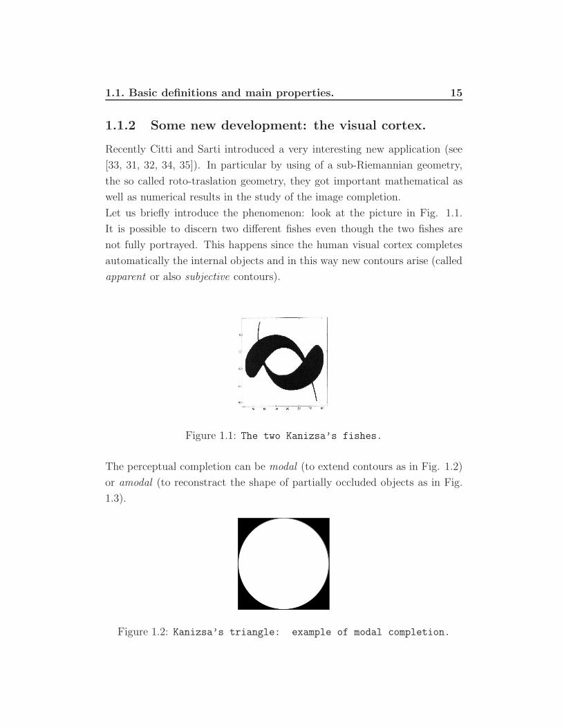
Let us briefly introduce the phenomenon: look at the picture in Fig. 1.1.
It is possible to discern two different fishes even though the two fishes are
not fully portrayed. This happens since the human visual cortex completes
automatically the internal objects and in this way new contours arise (called
apparent or also subjective contours).
Figure 1.1: The two Kanizsa’s fishes.
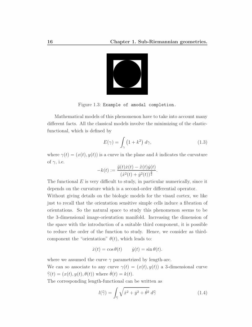
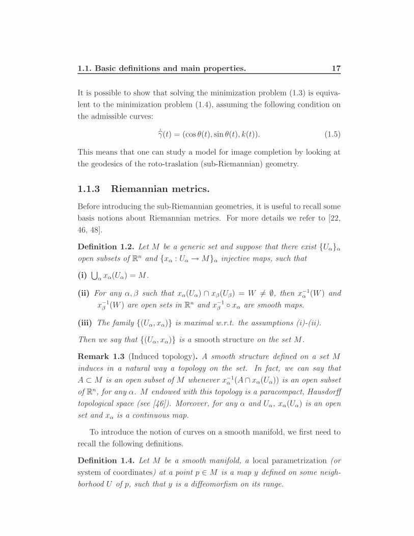
The perceptual completion can be modal (to extend contours as in Fig. 1.2)
or amodal (to reconstract the shape of partially occluded objects as in Fig.
1.3).
Figure 1.2: Kanizsa’s triangle: example of modal completion.
16 Chapter 1. Sub-Riemannian geometries.
Figure 1.3: Example of amodal completion.
Mathematical models of this phenomenon have to take into account many
different facts. All the classical models involve the minimizing of the elastic-
functional, which is defined by
E(γ) =
∫
γ
(1 + k2
)dγ, (1.3)
where γ(t) = (x(t), y(t)) is a curve in the plane and k indicates the curvature
of γ, i.e.
−k(t) :=y(t)x(t) − x(t)y(t)
(x2(t) + y2(t))32
.
The functional E is very difficult to study, in particular numerically, since it
depends on the curvature which is a second-order differential operator.
Without giving details on the biologic models for the visaul cortex, we like
just to recall that the orientation sensitive simple cells induce a fibration of
orientations. So the natural space to study this phenomenon seems to be
the 3-dimensional image-orientation manifold. Increasing the dimension of
the space with the introduction of a suitable third component, it is possible
to reduce the order of the function to study. Hence, we consider as third-
component the “orientation” θ(t), which leads to:
x(t) = cos θ(t) y(t) = sin θ(t).
where we assumed the curve γ parametrized by length-arc.
We can so associate to any curve γ(t) = (x(t), y(t)) a 3-dimensional curve
γ(t) = (x(t), y(t), θ(t)) where θ(t) = k(t).
The corresponding length-functional can be written as
l(γ) =
∫
bγ
√x2 + y2 + θ2 dγ (1.4)
1.1. Basic definitions and main properties. 17
It is possible to show that solving the minimization problem (1.3) is equiva-
lent to the minimization problem (1.4), assuming the following condition on
the admissible curves:
˙γ(t) = (cos θ(t), sin θ(t), k(t)). (1.5)
This means that one can study a model for image completion by looking at
the geodesics of the roto-traslation (sub-Riemannian) geometry.
1.1.3 Riemannian metrics.
Before introducing the sub-Riemannian geometries, it is useful to recall some
basis notions about Riemannian metrics. For more details we refer to [22,
46, 48].
Definition 1.2. Let M be a generic set and suppose that there exist Uαα
open subsets of Rn and xα : Uα → Mα injective maps, such that
(i)⋃
α xα(Uα) = M .
(ii) For any α, β such that xα(Uα) ∩ xβ(Uβ) = W 6= ∅, then x−1α (W ) and
x−1β (W ) are open sets in R
n and x−1β xα are smooth maps.
(iii) The family (Uα, xα) is maximal w.r.t. the assumptions (i)-(ii).
Then we say that (Uα, xα) is a smooth structure on the set M .
Remark 1.3 (Induced topology). A smooth structure defined on a set M
induces in a natural way a topology on the set. In fact, we can say that
A ⊂M is an open subset of M whenever x−1α (A∩ xα(Uα)) is an open subset
of Rn, for any α. M endowed with this topology is a paracompact, Hausdorff
topological space (see [46]). Moreover, for any α and Uα, xα(Uα) is an open
set and xα is a continuous map.
To introduce the notion of curves on a smooth manifold, we first need to
recall the following definitions.
Definition 1.4. Let M be a smooth manifold, a local parametrization (or
system of coordinates) at a point p ∈ M is a map y defined on some neigh-
borhood U of p, such that y is a diffeomorfism on its range.
18 Chapter 1. Sub-Riemannian geometries.
Definition 1.5. Let M1 and M2 be smooth manifolds with dimension n and
m respectively. A map φ : M1 → M2 is differentiable if and only if for any
p ∈M1 and for any local parametrization (V, y) at φ(p) ∈M2, there exists a
local parametrization (U, x) at p ∈M1 such that
(i) φ(x(U)) ⊂ y(V ),
(ii) y−1 φ x : U ⊂ Rn → V ⊂ Rm is a smooth map in x−1(p).
Next we introduce the notion of a curve on a smooth manifold.
Definition 1.6. Let M be a smooth manifold and I a real interval, then any
differentiable map γ : [0, T ] →M is a curve on M .
Let be γ(0) = p ∈ M and D be the set of all the functions which are
differentiable at the point p, then the following real functional
γ(0) : D −→ R
f 7−→ γ(0)f :=d(f γ)dt
∣∣t=0
(1.6)
is a tangent vector at the point p ∈M .
Definition 1.7. We call tangent space to the smooth manifold M at a point
p the set of all the tangent vectors at the point p, i.e.
TpM := γ(0)| γ(0) satisfying (1.6) and γ(0) = p. (1.7)
Remark 1.8. If M is a n-dimensional smooth manifold, then for any point
p ∈M the tangent space TpM is a n-dimensional space.
Definition 1.9. Let M be a smooth manifold, we call tangent bundle of M
the following 2n-dimensional vector space:
TM := (p, v)| p ∈M, v ∈ TpM. (1.8)
Let M1 and M2 be two different smooth manifolds and let φ : M1 → M2
be a differentiable map between the two manifolds. By definition, for any
p ∈ M1 and v ∈ TpM1 there exists a curve γ : I → M1 such that γ(0) = p
and γ(0) = v, so β := φ γ defines a curve on the smooth manifold M2
1.1. Basic definitions and main properties. 19
with β(0) = φ(p) ∈ M2. We can so define a linear map between the two
corresponding tangent bundles TM1 and TM2 by considering
dφp : TpM1 −→ Tφ(p)M2
v 7−→ dφp(v) := β(0). (1.9)
The previous map is well-defined, since it does not depend on the chosen
curve. More details on this remark can be found in [46].
Definition 1.10. Let M1 and M2 be two smooth manifolds and φ : M1 →M2
a differentiable map, the linear map dφp defined by (1.9) is called differential
of φ at the point p.
We now introduce the notion of a Riemannian metric, by using a system
of local coordinates.
Definition 1.11 (Riemannian metric). A Riemannian metric on a smooth
manifold M is an application from a point p ∈ M to an inner product 〈 , 〉pdefined on the tangent space TpM , which “changes in a differentiable way”,
i.e. such that, given a local coordinate map x : U ⊂ Rn → M around
p ∈ M and given a point q = x(x1, ..., xn) ∈ x(U), then, set ∂∂xi
(q) =
dxq(0, ..., 1, ..., 0), the following function
gi j(x1, ..., xn) :=
⟨∂
∂xi(q),
∂
∂xj(q)
⟩
q
,
is differentiable on whole U .
The function gi j is called local representation of the Riemannian metric
w.r.t. the system of local coordinates x : U ⊂ Rn →M .
Note also that a smooth manifold with a Riemannian metric defined on is
usually called Riemannian manifold.
Remark 1.12. In general we indicate an inner product simply as⟨,⟩
(i.e.
omitting the base-point).
Remark 1.13. To characterize a Riemannian metric, we can equivalently
require that for any couple of differential vector fields X, Y defined on the
smooth manifold M the function 〈X, Y 〉 is (locally) differentiable on M .
20 Chapter 1. Sub-Riemannian geometries.
The following theorem is one of the main result on the theory of Rieman-
nian manifolds.
Theorem 1.14 ([46]). On any Hausdorff, smooth manifold with a countable
basis, it is always possible to define a Riemannian metric on.
In order to introduce a notion of geodesics, we need first to define the
length of curves.
Definition 1.15. Let(M, 〈 , 〉
)be a Riemannian manifold and γ : [0, T ] →
M an absolutely continuous curve, we call length of the curve γ the following
real functional
l(γ) :=
∫ T
0
⟨γ(t), γ(t)
⟩ 12dt. (1.10)
Definition 1.16. Let(M, 〈 , 〉
)be a Riemannian manifold and p, q ∈ M ,
the (Riemannian) distance between these two points is defined as
d(p, q) := infl(γ) | γ a.c. curve, joining p to q. (1.11)
The geodesics are usually defined as the curves with vanishing acceler-
ation. To make formal this definition, we have to say what we mean by
acceleration, and so we need to introduce the so called Levi-Civita connec-
tion and covariant derivatives. Nevertheless, it is possible to show that all
the curves with minimum-length (i.e. curves realizing the distance (1.11)) are
geodesics. The inverse claim is not true. In fact, if one thinks of a sphere and
two its no-antipodal points, there are two different arcs of maximum-circle
joining them. Since any maximum-circle has vanishing acceleration, there
are two different geodesics joining these two points but only one realizes the
distance. Usually, the curves, minimizing the length are called minimizing
geodesics. By geodesics we will always refer to these minimizing curves.
Theorem 1.17 (Existence and uniqueness). Let M be a Riemannian man-
ifold and p0 ∈ M , for any ε > 0, there exists a neighborhood U of p0 such
that for any p ∈ U there exists a unique (minimizing) geodesic, joining p0 to
p with length less or equal to ε.
Moreover, if the Riemannian manifold M is complete, then there exists at
least a geodesic joining any pair of points.
1.1. Basic definitions and main properties. 21
In order to get some global existence-result, the assumption of complete-
ness is necessary. In fact, if one looks at R\0 with the Euclidean metric
there are not geodesics joining two opposite points p and −p.
1.1.4 Carnot-Caratheodory metrics and the Horman-
der condition.
The main difference between Riemannian and sub-Riemannian geometries is
that in the sub-Riemannian case not every curve is admissible. In this section
we want to introduce a rigorous mathematical defintion of sub-Riemannian
geometry and study their main properties.
Definition 1.18. Let M be a n-dimensional smooth manifold and r ≤ n,
a r-dimensional distribution H is a subbundle of the tangent bundle, i.e.
H := (p, v) | p ∈ M, v ∈ H(p), where H(p) is a r-dimensional subspace of
the tangent space at the point p.
Remark 1.19. Note that sometimes the dimension of the distribution (which
can be called also rank) can depend on the point p (see Example 1.22).
Nevertheless the main sub-Riemannian geometries are associated to rank-
constant distributions. E.g. the Heisenberg group and more in general any
Carnot group (see Sec.1.3 and Sec.1.2).
Definition 1.20 (Sub-Riemannian metric). Let M be a smooth manifold and
H ⊂ TM a distribution, a sub-Riemannian metric on M is a Riemannian
metric defined on the fibers of the subbundle H.
Definition 1.21 (Sub-Riemannian geometry). A sub-Riemannian geometry
is a tern(M,H, 〈 , 〉
), where M is a smooth manifold, H is a distribution,
and 〈 , 〉 is a Riemannian metric defined on H.
From now on, we indicate by X1, ..., Xm the vector fields spanning the
distribution H, i.e.
H(p) = Span(X1(p), ..., Xm(p)),
at any point p ∈M .
22 Chapter 1. Sub-Riemannian geometries.
Example 1.22. The Grusin plane is the sub-Riemannian geometry defined
on R2 by the distribution spanned by the two 2-dimensional vector fields
X(p) = (1, 0)t and Y (p) = (0, x1)t, with p = (x1, x2) ∈ R2, endowed with
the real Euclidean metric. Note that r(p) = 1, at the origin, while r(p) = 2,
otherwise.
It is possible to introduce a weak-linear-independent condition which
includes both the rank-constant distributions and the Grusin-type spaces
(which generalizes Example 1.22), assuming that for any p ∈ M there exist
1 ≤ r(p) ≤ m and 1 ≤ j1 < ... < jr(p) ≤ m such that
rankXj1(p), ..., Xjr(p)(p) = r(p), and Xj(p) = 0, ∀ j /∈ j1, ..., jr(p).
(1.12)
The fact that⟨,⟩
is defined only on H implies that we can define a notion
of length only for a particular class of curves.
Definition 1.23 (Horizontal curves). Let(M,H, 〈 , 〉
)be a sub-Riemannian
geometry and γ : [0, T ] → M an absolutely continuous, we say that γ is a
horizontal (or also admissible) curve if and only if
γ(t) ∈ Hγ(t), for a.e. t ∈ [0, t],
or equivalently, if there exists a measurable function h : [0, T ] → Rm such
that
γ(t) =m∑
i=1
hi(t)Xi(γ(t)), for a.e. t ∈ [0, t],
where h(t) = (h1(t), . . . , hm(t)).
For the horizontal curves and only for those, it is possible to define a
length-functional as
l(γ) :=
∫ T
0
‖γ(t)‖ dt, (1.13)
where ‖γ(t)‖ = 〈γ(t), γ(t)〉 12 .
Exactly as in the Riemannian case, by using the length for the horizontal
curves we can introduce a notion of distance on the manifold.
1.1. Basic definitions and main properties. 23
Definition 1.24 (Carnot-Caratheodory distance). We call sub-Riemannian
distance or also Carnot-Caratheodory distance the function d : M ×M →[0,+∞], defined by
d(p, q) := infl(γ)| γ horizontal curve joining p to q. (1.14)
Theorem 1.25. The function d(p, q) defined by (1.14) induces a distance on
the whole manifold M .
Proof. The symmetry is easy to show. In fact for any horizontal curve γ
which joins p to q in a time T , we can define the inverse curve γ(t) := γ(T−t).The curve γ is a horizontal curve joining q to p. Moreover l(γ) = l(γ) .
To show the triangular inequality, let us fix two points p, q ∈ M . First,
we consider the case d(p, q) < +∞. Given a third point z ∈ M , we can
always assume that d(p, z)d(z, q) < +∞. In fact, whenever d(p, z) = +∞or d(z, q) = +∞, the triangular inequality is trivially satisfied. Then, given
two horizontal curves γ1 and γ2 joining respectively p to z and z to q, we can
consider the attached path γ := γ1 ∨ γ2.
It is immediate to note that γ is still an horizontal curve. Moreover, γ joins
p to q and l(γ) ≤ l(γ1) + l(γ2). Therefore
d(p, q) ≤ d(p, z) + d(z, q). (1.15)
The remaining case d(p, q) = +∞ is trivail to prove. One has just to remark
that, for any third point z ∈ M , then d(p, z) = +∞ or d(z, q) = +∞. In
fact, if we assume that d(p, z)d(z, q) < +∞, then there exist two horizontal
curves γ1 and γ2, both having a finite length, joining respectively p to z and
z to q. So the attached curve γ (defined as above) is an horizontal curve
joining p to q and with l(γ), which implies d(p, q) ≤ l(γ) < +∞, which leads
to a contradiction.
Note that, since the length-functional is non-negative, then it d(p, q) ≥ 0
for any p, q ∈ M . We only remain to prove that d(p, q) = 0 if and only if
p = q. This result is a consequence of the local Euclidean estimate for Carnot-
Carateodory distances, which we are going to prove in the next subsection
24 Chapter 1. Sub-Riemannian geometries.
(see Lemma 1.44 and Remark 1.45). Therefore, so far we omit the proof of
this property.
Nevertheless it could happen that there is not any horizontal curve joining
two given points. In this case the sub-Riemannian distance between these
points is infinite. So we need to introduce a condition ensuring that the
distance between two points is always finite.
At this purpose, let us recall that given two vector fields X, Y defined on
some manifold M , the bracket between X and Y is the vector field defined
as [X, Y ] := XY − Y X, i.e. actioning on smooth functions f : M → R by
derivation as
[X, Y ](f) = X(Y (f)) − Y (X(f)).
Example 1.26. Let be M = R2, we set p = (x, y) ∈ R2, and consider the
two vector fields X(x, y) = (1, 0)t and Y (x, y) = (0, x)t. Then
[X, Y ](f) = x∂2
∂x∂yf(x, y) − ∂
∂yf(x, y) − x
∂2
∂y∂xf(x, y) = − ∂
∂yf(x, y).
By induction, a k-length bracket is a vector field defined as [Zi, Z(k−1)j ],
where Zi ∈ X, Y and Z(k−1)j is a bracket between X and Y with length
less or equal to k− 1. For example the 2-length-brackets between two vector
fields X and Y are given by [X, [X, Y ]], [X, [Y,X]], [Y, [X, Y ]], [Y, [Y,X]].
Note that [X, Y ] = −[Y,X], hence [X, Y ] = [Y,X] if and only if
[X, Y ] = 0, i.e. if and only if the two vector fields commute.
Let us consider a family of vector fields X = X1, ..., Xm spanning some
distribution H ⊂ TM , the associated Lie algebra is the set of all the brackets
between the vector fields of the family, i.e.
L(X ) := [Xi, X(k)j ] | X(k)
j k − length bracket ofX1, ..., Xm, k ∈ N.
Definition 1.27. Let M be a smooth manifold and H a distribution defined
on M . We say that the distribution is bracket-generating if and only if, at
any point, the Lie algebra L(X ) spans the whole tangent space.
1.1. Basic definitions and main properties. 25
Definition 1.28 (Hormander condition). We say that a sub-Riemannian
geometry satisfies the Hormander condition if and only if the associated dis-
tribution is bracket generating.
Theorem 1.29 (Chow’s Theorem). Let M be a smooth manifold and H a
bracket generating distribution defined on M . If M is connected, then there
exists a horizontal curve joining two given points of M .
From Chow’s Theorem it follows that, whenever a sub-Riemannian ge-
ometry satisfies the Hormander condition, the distance defined by (1.14) is
finite at any pair of points. In the Subsection 1.1.6, we are going to give
more details on Chow’s Theorem and show an easy proof in the particular
case of the Heisenberg group.
To introduce the notion of step of a bracket generating distribution, let us
introduce the following notion. Let H be a family of vector fields, we write:
L1 := Span(Z = X |X ∈ H),L2 := Span(Z = [X, Y ] |X, Y ∈ L1),. . . . . . . . . . . . . . . . . . . . .
Li = Span(Z = [X, Y ] |X ∈ H, Y ∈ Li−1).
(1.16)
Moreover, we indicate by Li(p) the vector space corresponding to Li evalu-
ated at the point p ∈M .
Definition 1.30 (Step of a distribution). Let X = X1, ..., Xm be a family
of vector fields defined on a smooth manifold M and H the distribution gen-
erated by X1, ..., Xm. Given p ∈ M , we call step of the distribution H at the
point p, and we indicate by k(p), the smallest natural number such that
k(p)⋃
i=1
Li(p) = TpM.
Example 1.31. Any Riemannian geometry is bracket generating with step
equal to 1 at any point. In fact(M,H,
⟨,⟩)
is a Riemannian manifold if
and only if H = TM (which means L1(p) = TpM for any p ∈M).
Example 1.32. The Heisenberg group is associated to a bracket generating
with step equal to 2 at any point (see Definition 1.106).
26 Chapter 1. Sub-Riemannian geometries.
Example 1.33. The Grusin plane is associated to a bracket generating with
step 2 at the origin, and with step 1 otherwise (see Definition 1.22).
The reverse implication of Chow’s Theorem (“finite distance implies the
Hormander condition”) holds only for analytic distributions but it is in gen-
eral false for smooth distributions, see the following counter-example.
Example 1.34. Look at the sub-Riemannian metric generated by the 2-
dimensional vector fields X = (1, 0)t and Y = (0, a(x))t, with a ∈ C∞(R)
such that a(x) = 0, if x ≤ 0, and a(x) > 0, if x > 0, so that X, Y are
smooth vector fields. The corresponding sub-Riemannian distance is finite.
Nevertheless, the associated distribution is not bracket generating. In fact, if
x ≤ 0, then Y = (0, 0)t and so Span(L(X, Y )(p)) = Span(X(p)) 6= R2.
Example 1.35. Let X and Y be as in the Example 1.34, but with a(x) = 1
if x ≥ 0, and a(x) = 0 if x < 0. In this case a 6∈ C∞(R), however, we can
use this example in order to investigate the previous one.
On the half-plane x < 0, we can move only in one direction, then the spanned
distribution is not bracket generating.
Nevertheless, it is easy to write explicitly the associated Carnot-Caratheodory
distance, that is
d((x, y), (x′, y′)) =
√|x− y|2 + |x′ − y′|2, x1 ≥ 0 x′ ≥ 0,
|x| + |x′| + |y − y′|, x < 0 x′ < 0,
|x| +√|x′|2 + |y − y′|2, x < 0 x′ ≥ 0,
|x′| +√
|x|2 + |y − y′|2, x ≥ 0 x′ < 0.
It is immediate to note that d(x, y) is a finite distance.
Remark 1.36 (Involutive distributions). The opposite case to the bracket
generating distributions is given by the so called involutive distributions. We
recall that a distribution H is said involutive if and only if [X, Y ] ∈ H, for
any X, Y ∈ H. By the Frobenius Theorem (see [50]), it is known that, if
M is a n-dimensional smooth manifold and H is a r-dimensional involutive
distribution defined on M , then, given p ∈ M , the set of all the horizontal
curves through a fixed point p, is an immerse r-dimensional submanifold,

1.1. Basic definitions and main properties. 27
called leaf. Therefore, if q ∈ M does not belong to the lift of p, there is not
any horizontal curve joining p to q. So, in this case, d(p, q) = +∞.
In particular, if r < n such a point q always exists.
1.1.5 Notions equivalent to the Carnot-Caratheodory
distance.
Next we want to intorduce a notion of distance equivalent to the Carnot-
Caratheodory distance. This new distance is very used in control theory and
so it is often called control distance (or also minimal time distance). Let
X = X1, ..., Xm be smooth vector fields generating a distribution H, we
recall that an absolutely continuous curve γ : [0, T ] →M is horizontal if and
only if
γ(t) =m∑
i=1
hi(t)Xi(γ(t)), a.e. t ∈ [0, T ], (1.17)
for suitable hi(t) measurable functions. We can think of (1.17) as a control
system, which we know to be well-posed whenever hi ∈ L1([0, T ]). We like
to recall that in control theory the functions hi are usually called control
functions while the solutions of (1.17) are called control paths.
Remark 1.37. If the vector fields X1, ..., Xm are linearly independent at any
point, then the coordinates hi are unique. Moreover the uniqueness still holds
if we assume the weak-linearly-independent-condition (1.12).
Under assumption (1.12), we can define the length of a horizontal curve
γ : [0, T ] →M , by using the local coordinates hi, i.e.
l(γ) =
∫ T
0
(h2
1(t) + ... + h2m(t)
) 12dt. (1.18)
Remark 1.38. In general, the control functions hi can be non-unique. In
such a case, we define the length-functional taking the infimum of (1.18) over
all the admissible coordinates hi. More precisely, h1, ..., hm are admissible
coordinates if and only if they satisfy (1.17) and, moreover, h1, ..., hm ∈L1([0, T ]) (otherwise the corresponding integral is equal to +∞). This implies
l(γ) = inf
∫ T
0
((h1(t))
2 + ... + (hm(t))2) 12 dt
∣∣∣∣hi ∈ L1([0, T ]) satisfying (1.17)
.

28 Chapter 1. Sub-Riemannian geometries.
We so can re-write the sub-Riemannian distance defined in (1.14) by us-
ing the local expression (1.18).
Next we introduce a definition of sub-Riemannian distance as suitable mini-
mal time function.
Definition 1.39. We say that a horizontal curve γ : [0, T ] → M is subunit
if and only if the coordinates given by (1.17) are such that
m∑
i=1
h2i (t) ≤ 1, a.e. t ∈ [0, T ].
Definition 1.40. For any x, y ∈ M , we look at the following minimal time
function:
d(x, y) = infT | ∃ γ : [0, T ] →M a.c. subunit hor. curve joining x to y.(1.19)
Proposition 1.41 ([76], Proposition 1.1.10). The function d(x, y) defines a
distance on the smooth manifold M .
We want to show that the minimal time distance d(x, y) is equivalent
to the Carnot-Carathodory distance. This is a consequence of the following
result.
Theorem 1.42 ([76]). Let γ be a horizontal curve and, let us assume for
sake of simplicity that T = 1. If h = (h1, ..., hm)t are the local coordinates of
γ w.r.t. X1, ..., Xm, then for any 1 ≤ p ≤ +∞ we can define a distance on
M by
dp(x, y) = inflp(γ) | γ : [0, 1] →M a.c. hor. curve joining x to y, (1.20)
with
lp(γ) := ‖h‖p =
(∫ 1
0
|h(t)|pdt) 1
p
, if 1 ≤ p < +∞,
ess. supt∈[0,1]
|h(t)|, if p = +∞,
where the essential supremum of h(t) is defined by
ess. supt∈[0,1]
|h(t)| = infM ≥ 0 | |h(t)| ≤M, a.e. t ∈ [0, 1]
.
Then dp(x, y) = d(x, y) for any x, y ∈M and for any 1 ≤ p ≤ +∞.
1.1. Basic definitions and main properties. 29
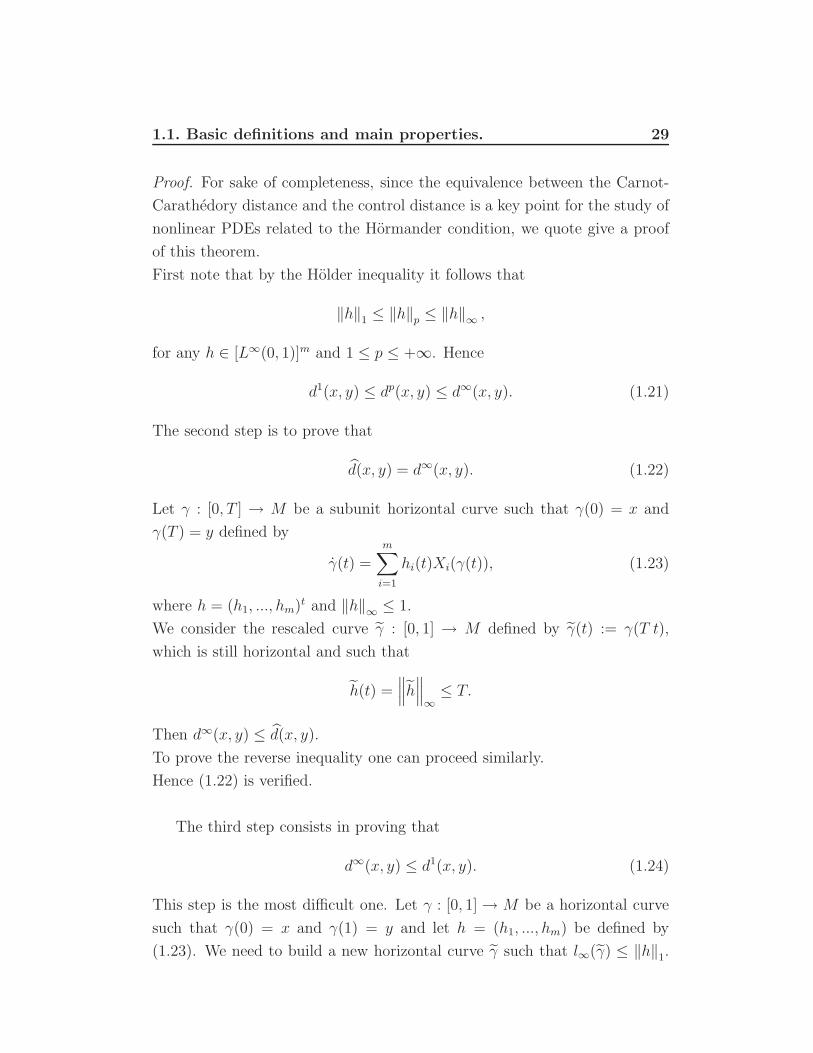
Proof. For sake of completeness, since the equivalence between the Carnot-
Carathedory distance and the control distance is a key point for the study of
nonlinear PDEs related to the Hormander condition, we quote give a proof
of this theorem.
First note that by the Holder inequality it follows that
‖h‖1 ≤ ‖h‖p ≤ ‖h‖∞ ,
for any h ∈ [L∞(0, 1)]m and 1 ≤ p ≤ +∞. Hence
d1(x, y) ≤ dp(x, y) ≤ d∞(x, y). (1.21)
The second step is to prove that
d(x, y) = d∞(x, y). (1.22)
Let γ : [0, T ] → M be a subunit horizontal curve such that γ(0) = x and
γ(T ) = y defined by
γ(t) =
m∑
i=1
hi(t)Xi(γ(t)), (1.23)
where h = (h1, ..., hm)t and ‖h‖∞ ≤ 1.
We consider the rescaled curve γ : [0, 1] → M defined by γ(t) := γ(T t),
which is still horizontal and such that
h(t) =∥∥∥h∥∥∥∞
≤ T.
Then d∞(x, y) ≤ d(x, y).
To prove the reverse inequality one can proceed similarly.
Hence (1.22) is verified.
The third step consists in proving that
d∞(x, y) ≤ d1(x, y). (1.24)
This step is the most difficult one. Let γ : [0, 1] → M be a horizontal curve
such that γ(0) = x and γ(1) = y and let h = (h1, ..., hm) be defined by
(1.23). We need to build a new horizontal curve γ such that l∞(γ) ≤ ‖h‖1.
30 Chapter 1. Sub-Riemannian geometries.
Suppose that ‖h‖1 > 0 and let φ : [0, 1] → [0, 1] be the following absolutely
continuous function:
φ(t) =1
‖h‖1
∫ t
0
|h(τ)|dτ,
φ is non decreasing and its “inverse function” ψ : [0, 1] → [0, 1] defined as
ψ(s) = inft ∈ [0, 1]|φ(t) = s
is a monotone function, too. So it is differentiable a.e. s ∈ [0, 1].
We want to prove that
φ(ψ(s))ψ(s) = 1, a.e. s ∈ [0, 1]. (1.25)
Therefore we define
B = t ∈ [0, 1] |φ is not differentiable in t
and
D = t ∈ [0, 1] |φ is not differentiable inψ(t).Since φ is an absolutely continuous function, it is such that vanishing-measure
sets go into vanishing-measure sets, i.e. |B| = 0 implies |φ(B)| = 0.
Moreover D ⊂ φ(B), so |D| = 0 and then we have (1.25).
So we can define γ(s) := γ(ψ(s)). Now, let be
E = t ∈ [0, 1] | γ is not differentiable inψ(t),
γ is absolutely continuous, then the previous argument shows also that |E| =
0. Hence
˙γ(s) = γ(ψ(s))ψ(s) =m∑
i=1
hi(ψ(s))ψ(s)Xi(γ(s)), a.e. s ∈ [0, 1].
If |h(ψ(s))| 6= 0, it is trivial to remark that
ψ(s) =1
φ(ψ(s)) =
‖h‖1
|h(s)| .
We can define
hi(s) =
‖h‖1
hi(ψ(s))
|h(ψ(s))| , if |h(ψ(s))| 6= 0,
0, if |h(ψ(s))| = 0.
1.1. Basic definitions and main properties. 31
Setting
˙γ(s) =
m∑
i=1
hi(s)Xi(γ(s)), a.e. s ∈ [0, 1],
we get a horizontal curve such that∥∥∥h∥∥∥∞
≤ ‖h‖1 ,
so that (1.24) holds. Hence, by estimate (1.21), we can conclude
d∞(x, y) = d1(x, y) = dp(x, y),
for any 1 ≤ p ≤ +∞, and, therefore, by (1.22), we get d(x, y) = dp(x, y), for
any x, y ∈M .
Corollary 1.43. The Carnot-Caratheodory distance d(x, y) defined by (1.14)
is equivalent to the minimal time distance d(x, y) defined by (1.19).
Proof. The Theorem 1.42 with p = 1 implies that d1(x, y) = d(x, y). We need
only to recall that the Euclidean norm of Rm is equivalent to the norm defined
as |(h1, ..., hm)| = |h1|+ ...+ |hm|. This implies that d1(x, y) is equivalent to
d(x, y) and then d(x, y) is so.
To conclude this subsection, we show an Euclidean estimate from be-
low for the sub-Riemannian distance d(x, y). Note that, since the distances
d(x, y) and d(x, y) are equivalent, the same estimate holds for d(x, y).
Lemma 1.44. Let M be a smooth manifold and X = X1, ..., Xm smooth
vector fields generating a distribution H and satisfying the Hormander condi-
tion with step equal to k ≥ 1. If d(x, y) is the minimal time distance defined
by (1.19), then for any K ⊂ M compact there exists a constant C > 0 such
that
C|x− y| ≤ d(x, y), for any x, y ∈ K. (1.26)
Proof. Let us fix a compact set K and choose 0 < ε << 1 such that
Kε =
z ∈ M
∣∣∣∣ minx∈K
|z − x| ≤ ε
⊂⊂ M.
At any point x ∈M we can define a n×m-matrix by
A(x) := [X1(x), ..., Xm(x)],
32 Chapter 1. Sub-Riemannian geometries.
and
M = supx∈Kε
‖A(x)‖ ,
where by ‖ ‖ we indicate the usual norm of matrices.
Fix x, y ∈ K and let γ : [0, T ] → M be a subunit horizontal curve such that
γ(0) = x and γ(T ) = y.
Note that, by the Hormander condition, such a curve γ always exists. Then
we set r = minε, |x− y| so that TM ≥ r (one can find a detailed proof of
this claim in [76], Lemma 1.1.8).
Therefore, if we choose r = ε and consider the diameter D of K defined as
D := sup|x− y| | x, y ∈ K,
we get
T ≥ ε
M≥ ε
MD|x− y|. (1.27)
While, if we choose r = |x− y|, we find
T ≥ |x− y|M
. (1.28)
Since γ is an arbitrary subunit horizontal curve joining x to y, from (1.27)
and (1.28) it follows that
d(x, y) ≥ min
1
M,ε
MD
|x− y|.
Passing to the limit, as ε → 0+ we get estimate (1.26).
Remark 1.45. From the previous estimate, it follows that the sub-
Riemannian distance d(x, y) is positive definite, so this remark concludes
the proof of Proposition 1.25.
In Sec.1.1.7 we will show that there exists also an Euclidean estimate
from above but it is an Holder-estimate while the estimate from below is
Lipschitz-estimate.

1.1. Basic definitions and main properties. 33
1.1.6 Chow’s Theorem.
Chow’s Theorem is the main result for bracket generating distributions. In
this subsection we want to give a sketch of the non-trivial proof of this re-
sult. Nevertheless, before proving the theorem in the general case, we like
to quote a very simple and nice proof by Gromov in [51], which holds in the
particular case of the 1-dimensional Heisenberg group. So we need to intro-
duce briefly the 1-dimensional Heisenberg group (more details will be given
in Sec.1.3). We call (1-dimensional) Heisenberg group the sub-Riemannian
geometry defined on R3 by the distribution H, associated to the vector fields
X =
1
0
−y2
, Y =
0
1x2
, for any (x, y, z) ∈ R
3,
and endowed with the standerd Euclidean metric (on R2).
Note that, if we consider the 1-form
η := dz − 1
2(xdy − ydx),
then H = ker(η).
We indicate the n-dimensional Hiesenberg group by Hn and by H
1 the 1-
dimensional Hiesenberg group.
Note that a curve γ : [0, T ] → R3 is H1-horizontal, if and only if, η(γ(t)) =
0, a.e. t ∈ [0, T ]. This definition is called the canonical definition of 1-
dimensional Heisenberg group.
There is also another definition: the polarized Heisenberg group. In Sec.1.3.3
we will show that these two definitions are indeed equivalent.
Gromov uses this second definition but we prefer to rewrite the Gromov’s
proof using the canonical definition.
Next we rewrite Chow’s Theorem in the particular case of the 1-dimensional
Heisenberg group.
Theorem 1.46. Given two points in R3, there exists an absolutely continuous
H1-horizontal curve joining them.
Proof. Let p = (x1, y1, z1) and q = (x2, y2, z2) be two given points of R3.
Let γ(t) = (x(t), y(t)) be a plane curve joining (x1, y1) to (x2, y2). For sake
34 Chapter 1. Sub-Riemannian geometries.
of simplicity we assume T = 1.
Remark that we can look only at the absolutely continuous curves with con-
stant curvature, i.e. we can assume that∫
eγ
xdy =
∫ 1
0
x(t)y(t)dt =1
2
∫ 1
0
(x(t)y(t) − y(t)x(t)
)dt = C,
for some C ∈ R.
Then we can define a curve in R3, setting γ(t) = (x(t), y(t), z(t)), where the
third-coordinate is given by
z(t) = z1 +1
2
∫ t
0
(x(s)y(s) − y(s)x(s)
)ds.
Obviously γ is an absolutely continuous curve in R3. Moreover, since z(0) =
z1 and z(1) = z1 − C, choosing C = z1 − z2, then γ joins p to q.
In order to conclude the proof, we need only to observe that, for a.e. t ∈ [0, 1],
it holds η(γ(t)) = 0 and so γ is a H1-horizontal curve.
To prove Theorem 1.29 in the general case is more difficult.
The general result was proved, almost contemporaneously but indipendently,
by Rashevsky in [82] (1938) and by Chow in [30] (1939). There are many
different proofs of this result. We choose to briefly sketch the proof given
in [17], by using the point-of-view of control theory. First we need to recall
some definitions. From now on we indicate by BdR(p) the open ball centered
at p with radius R, w.r.t. the metric d(x, y), i.e.
BdR(p) = q ∈M | d(p, q) < R.
Definition 1.47. Let M be a connected sub-Riemannian manifold and p ∈M , the accessible set Ap is the set of all the points of M joined to p by a
horizontal curve.
Definition 1.48. An immersed submanifold of a manifold M is a subset
A ⊂M endowed with a manifold structure such that
(i) the inclusion map i : A→M is an immersion,
(ii) any continuous map f : P → M , where P is a manifold, is continuous
when we consider the restriction map f : P → A, where A is endowed
with its manifold topology.
1.1. Basic definitions and main properties. 35
To prove Chow’s Theorem is equivalent to show that, under the Horman-
der condition, the accessible set of any points of the manifold coincides with
the manifold itself. The key is the following property for the accessible sets.
Theorem 1.49 (Sussmann-Stefan’s Theorem, [17]). Let M be a connected
smooth manifold, then for any p ∈ M the accessible set Ap is an immersed
submanifold.
By using Sussemann-Stefan’s Theorem, Chow’s Theorem follows imme-
diately.
Proof of Theorem 1.29. Fix p ∈M and look at the accessible set Ap.
Note that q ∈ Ap if and only if d(p, q) < +∞, so we can write Ap as union
of the open balls BdR(p). Then Ap is an open subset of M .
Moreover by Sussemann-Stefan’s Theorem we know that Ap is an immersed
submanifold of M , therefore the vectors fields X1, ...Xm can be seen also as
tangent bundles to the immersed submanifold, i.e.
X1, ...Xm ∈ TAp.
Remember that, if some vector fields belong to a tangent space, then also
their brackets belong to it. So
[Xi, Xj], [[Xi, Xj], Xk], ... ∈ TAp.
By the bracket generating condition, we have that TAp = TM , which in
particular implies that the two spaces have the same dimension. Since Ap is
an open immersed submanifold of M , whenever it has the same dimension
of the manifold, it must coincide with a connected component of M . M is
connected, so Ap = M and this conclude the proof of Chow’s Theorem.
36 Chapter 1. Sub-Riemannian geometries.
1.1.7 Relationship between the Carnot-Caratheodory
distance and the Euclidean distance.
Now we want to study the relationship between any sub-Riemannian
distance satisfying the Hormander condition and the Euclidean distance.
First, we show that both of these distances induce on Rn the same topology.
Then we prove the main (local) estimates for Carnot-Caratheodory distances.
One can find a proof of this topological result in [75] (Theorem 2.3,
Sec.I.2.5). There, the Author gets the equivalence of the two topologies,
directly from the Ball-box Theorem (Theorem 2.10, pages 29-30), fixing a
neighborhood basis in the sub-Riemannian topology and building a suitable
neighborhood basis in the original topology of the manifold. Nevertheless,
we choose to follow the approach given in [17].
So look at the control system (1.17) and let p be an initial point and Up T an
open neighborhood of the origin in L1([0, T ],Rm).
Definition 1.50. We call end-point map the function Ep : Up T → M ,
defined as h 7−→ xh(T ), where xh a solution of (1.17), w.r.t. the control
function h.
We quote the following result without giving any proof.
Theorem 1.51 (End-point mapping Theorem, [17]). Let M be a smooth
manifold, H a bracket generating distribution and d(x, y) the associated sub-
Riemannian distance. Then the end-point map is open.
By the End-point mapping Theorem, we can deduce the following result.
Theorem 1.52. Let M , H and d(x, y) be as in Theorem 1.51, then d(x, y)
induces on M the original topology defined on the manifold.
Proof. Note that BdR(p) is the image of the ball BR(0) in L1 under the end-
point map, then by the End-point mapping Theorem BdR(p) is an open set
in M .
In order to prove the inverse result, we need to fix a point p ∈ M and a
neighborhood U of p. Since the end-point map Ep is continuous at 0, so
1.1. Basic definitions and main properties. 37
there exists R > 0 such that Ep maps the ball BR(0) ⊂ L1 into U . Hence
any neighborhood U contains a ball BdR(p) and this concludes the proof.
The previous theorem applied in Rn endowed with the Euclidean topology
implies the compactness of the sub-Riemannian balls, whenever the associ-
ated distribution is bracket generating.
Corollary 1.53. Let H be a bracket generating distribution defined on Rn
and d(x, y) the associated sub-Riemannian distance. Then a closed d-ball
BdR(x) := y ∈ R
n | d(x, y) ≤ R, for some R > 0 and x ∈ Rn,
is compact in the n-dimensional Euclidean space.
Proof. Let τ1 be the topology induced by the metric d(x, y) and τ2 the Eu-
clidean topology. They are equivalent, if and only if, for any fixed x ∈ Rn,
there exist B1 and B2 neighborhood-basis, w.r.t. τ1 and τ2, respectively, such
that for all B ∈ B1 there exist U, V ∈ B2 with U ⊂ B ⊂ V .
We can set B1 = Bdε (x) | ε > 0 and B2 = Bε(x) | ε > 0, where we indicate
by Bdε (x) the ball w.r.t. the sub-Riemannian metric d(x, y), and by Bε(x)
the usual Euclidean ball, both of them centered at x, with radius ε. Then,
the equivalency of the two topologies implies that, for any x ∈ Rn and ε > 0,
there exist r, R > 0 such that
Br(x) ⊂ Bdε (x) ⊂ BR(x).
Therefore the d-balls are bounded sets, then Bdε (x) are compact w.r.t. the
Euclidean topology, for any ε > 0.
Remark 1.54. Remember that the two metrics induce the same topology but
they are not equivalent. In fact fixed y ∈ Rn, we get that the radii depend on
x and y. Hence, the two metrics in general are not equivalent.
Remark 1.55. Note that the Hormander condition is very important in order
to get the equivalence of the two topologies. In Example 1.35, we introduced
a finite sub-Riemannian distance, which does not satisfy the Hormander con-
dition. It is very easy to see that such a distance is discontinuous w.r.t. the
Euclidean topology. In fact, for any x < 0
lim|y|→0
d((x, 0), (x, y)) = 2|x| 6= 0.
38 Chapter 1. Sub-Riemannian geometries.
We give now the main estimates for Carnot-Caratheodory distances sat-
isfying the Hormander condition.
Theorem 1.56. Let d(x, y) be a sub-Riemannian distance defined on a
smooth manifold M and satisfying the Hormander condition with step k.
Then, for any compact K ⊂ M , there exist two constants C1 = C1(K) > 0
and C2 = C2(K) > 0 such that
C1|x− y| ≤ d(x, y) ≤ C2|x− y| 1k , (1.29)
for any x, y ∈ K.
Proof. The estimate from below is given in Lemma 1.44.
We remain to show the estimate from above using the Hormander condition
and introdusing a new distance equivalent to the Carnot-Caratheodory dis-
tance.
Let us recall that, thanks to the Hormander condition, any absolutely con-
tinuous curve γ satisfies
γ(t) =
n∑
i=1
hi(t)Yi(γ(t)), a.e. t, (1.30)
where hi are measurable functions and Yi is a basis of the tangent bundle
TM , where only brackets between the elements X1, ..., Xm and with length
less or equal to k, appear (for more details see e.g. [17]).
Let C(δ) be the set of all the absolutely continuous curves γ : [0, 1] → M
such that (1.30) holds with |hi(t)| < δs for i = 1, ..., n and Yi ∈ Ls (i.e. Yi is
a bracket with length equal to s). Then we define a distance ρ by
ρ(x, y) = infδ > 0| ∃ γ ∈ C(δ) : γ(0) = x, γ(1) = y.
Fixed a compact K and two points x, y ∈ K, there exists an absolutely
continuous curve γ : [0, 1] →M , joining x to y and such that |γ(t)| ≤ C|x−y|,for suitable constant C = C(K) and for a.e. t ∈ [0, 1].
From (1.30), it follows that
|hi(t)| ≤ C1|γ(t)| ≤ C2|x− y| = C2
(|x− y| 1s
)s,
1.1. Basic definitions and main properties. 39
whenever Yi ∈ Ls. Since 0 < s ≤ k, we have proved that
ρ(x, y) ≤ C|x− y| 1k .
The distance ρ is equivalent to the Carnot-Caratheodory distance d(x, y) (see
[78], Theorem 4) and this concludes the proof.
Remark 1.57. Estimate (1.29) implies that the two metrics are equivalent
whenever k = 1, that is the Riemannian case.
1.1.8 Sub-Riemannian geodesics.
In this subsection we are going to intorduce and study sub-Riemannian
geodesics.
Definition 1.58 (Geodesic). A minimizing geodesic (or simply geodesic)
between two points x and y is any absolutely continuous horizontal curve
which realizes the distance (1.14).
As we have briefly remarked in the section about the Dido’s problem and
the perceptual visual completion, sub-Riemannian geodesics can be used in
order to solve minimization problems of the calculus of variations.
Exactly as in the Riemannian case, the geodesics can be found also min-
imizing the energy E among all the horizontal curves instead of the length-
functional (1.13). Let us give more details on this point.
Definition 1.59. Let γ : [0, T ] → M be an absolutely continuous horizontal
curve, we call energy of γ the following functional:
E(γ) =
∫ T
0
1
2‖γ(t)‖2 dt =
1
2
∫ T
0
⟨γ(t), γ(t)
⟩dt. (1.31)
By the Cauchy-Schwartz inequality, it follows that
∫fg ≤
√∫f 2
√∫g2,
40 Chapter 1. Sub-Riemannian geometries.
with the identity true if and only if f = cg for some constant c.
If we apply the previous inequality to the functions f = ‖γ‖ and g = 1, we
get that, for any horizontal curve γ : [0, T ] → M , it holds
l(γ) =
∫ T
0
‖γ(t)‖ dt ≤√T
√∫ T
0
‖γ(t)‖2 dt =√T√
2E(γ).
From this remark, we find the following result.
Proposition 1.60 ([75]). A curve γ minimizes the energy-functional E
among all the horizontal curves joining q to p in a time T if and only if
γ minimizes the length-functional among all the horizontal curves joining q
to p, parameterized by the constant-time c = d(p, q)/T .
Since the length of a curve does not depend on the chosen parametriza-
tion, we can always restrict to looking at the infimum only among the curves
with the previous constant parametrization. Therefore, by Proposition
(1.60) it follows that minimizing the energy or minimizing the length is
equivalent.
We now introduce equations to compute the geodesics in sub-Riemannian
geometries. At this purpose, we need to associate a Hamiltonian to a given
sub-Riemannian geometry.
We define the map β : T ∗M → TM acting as p(βx(q)) = 〈〈p, q〉〉x, for any
p, q ∈ T ∗M and x ∈M , where by 〈〈 , 〉〉 we indicate the cometric associated
to the sub-Riemannian metric⟨,⟩
Remark 1.61 ([75]). The map β associated to a sub-Riemannian geometry(M,H,
⟨,⟩)
is uniquely defined by the following two conditions:
1. Im(βx) = Hx,
2. p(v) = 〈βx(p), v〉 for any v ∈ Hx and any p ∈ T ∗M .
Definition 1.62 (Hamiltonian). The quadratic form
H(x, p) =1
2〈p, p〉x (1.32)
is called sub-Riemannian Hamiltonian (or also kinetic energy).
1.1. Basic definitions and main properties. 41
Suppose that γ is a horizontal curve, then there exists p ∈ T ∗M such that
γ(t) = βγ(t)(p) and1
2‖γ‖2 = H(γ(t), p). (1.33)
By the uniqueness of the map β, we get the following characterization for
sub-Riemannian geometries.
Proposition 1.63 ([75], Proposition 1.10). Any sub-Riemannian geometry
is uniquely determinate by its Hamiltonian. Conversely, any non-negative
quadratic Hamiltonian with constant rank k ≥ 1 defines a unique sub-
Riemannian structure associated to a k-rank-constant distribution.
To get the equations of geodesics, we introduce the momentum.
Definition 1.64. Let X be a vector field defined on a smooth manifold M ,
we call momentum of X the following functional defined on the cotangent
space:
PX(x, p) = p(X(x)), (1.34)
for any p ∈ T ∗M and x ∈M .
Let Xαα be a family of vector fields spanning the distribution H. If
we look at some system of local coordinates xi defined on M , then we know
that it is possible to express the vector fields Xα as
Xα(x) =n∑
i=1
X iα(x)
∂
∂xi
.
The corresponding momentum can be written as
PXα(x, p) =
n∑
i=1
X iα(x)P ∂
∂xi
,
where P ∂∂xi
are the momenta w.r.t. the coordinates vector fields.
Set pi = P∂/∂xi, (xi, pi) is a system of local coordinates on the cotangent
bundle T ∗M , usually called canonic coordinates.
We define the matrix (gα δ)α,δ as
gα δ = 〈Xα(x), Xδ(x)〉x
42 Chapter 1. Sub-Riemannian geometries.
and we indicate by gαδ the coefficients of the inverse matrix.
We get so the following explicit formulation for the Hamiltonian H in (1.32):
H(x, p) =1
2
∑
α, δ
gαδ(x)Pα(x, p)Pδ(x, p). (1.35)
Remark 1.65. In particular, if Xαα is an orthonormal system w.r.t. the
sub-Riemannian metric⟨,⟩, then (1.35) can be simplified as
H(x, p) =1
2
∑
α
P 2α(x, p), (1.36)
or equivalently, using the canonic coordinates, as
H(x, p) =1
2
∑
α
〈Xα(x), p〉2 . (1.37)
By (1.37) we get the following system of first-order differential equations
(defined on the cotangent bundle T ∗M):
xi =∂H
∂pi,
pi = −∂H∂xi
.
(1.38)
Definition 1.66. The Hamiltonian system (1.38) is called equations of the
normal geodesics.
Theorem 1.67. Let ζ(t) =(γ(t), p(t)
)be a solution of the Hamiltonian
system (1.38). Then, any short enough arc of γ(t) is a geodesic.
Definition 1.68 (Normal geodesics). Let ζ(t) =(γ(t), p(t)
)be a solution
of the Hamiltonian system (1.38), γ(t) is called (sub-Riemannian) normal
geodesic.
Exactly as in the Riemannian case, not all the normal geodesics are (min-
imizing) geodesics.
Nevertheless in the Riemannian geometries, all the (minimizing) geodesics
satisfy the equations of normal geodesics, while in the sub-Riemannian case,
there exists geodesics that are not normal geodesics.
1.1. Basic definitions and main properties. 43
Remark 1.69 (Singular geodesics). In the sub-Riemannian case, there are
geodesics that are not normal geodesics, i.e. that cannot be found as solutions
of the Hamiltonian system (1.38). Note that, if ζ(t) solves the system (1.38),
then H(γ(t), p(t)) is constant. Any geodesic γ(t) solving
H(γ(t), p(t)) = 0,
is called singular geodesic. Such a geodesic does not solves the system (1.38).
(Recall that by p(t) we indicate the dual variable of γ(t)).
Singular geodesics are usually more difficult to study than normal
geodesics. Nevertheless, in the case of contact distributions, all the geodesics
are normal. We recall that a distribution H is a contact distribution if and
only if it is defined by the kernel of a single one-form η with the property
that the restriction on any vector space H(p), dη∣∣H(p)
, is symplectic (i.e. non
degenerate) for any point p ∈ M . E.g. the Heisenberg group is a contact
distribution. So the Heisenberg group does not have any singular geodesic.
Next we give two examples of distributions admitting singular geodesics.
Example 1.70. Let us assume M = R3, we define H as the distribution
spanned at any point (x, y, z) ∈ R3 by X1 = (1, 0, 0)t and X2 = (0, 1−x, x2)t.
We look at the horizontal curve γ : [0, T ] → R3 defined as γ(t) = (0, t, 0).
The associated Hamiltonian is
H((x, y, z), (p1, p2, p3)) = −1
2
(p2
1 + (p2(1 − x) + p3x2)2).
So it is easy to verify that γ does not satisfy the equation of normal geodesics.
Nevertheless, if the interval is small enough, then γ is a geodesic (see [72],
Sec.2.3).
Example 1.71 (Martinet distribution). Let be M = R3 and X1 =
(1, 0,−y2)t and X2 = (0, 1, 0) for (x, y, z) ∈ R3. The distribution Hspanned by the vector fields X1 and X2 is known as Martinet distribu-
tion. It is a bracket generating distribution with step equal to 3 (in fact,
[X1, X2] = (1, 0,−2y)t and [[X1, X2], X2] = (0, 0,−2)t). The existence of sin-
gular geodesics in the Martinet distribution is given in [75], Theorem III.3.4.
44 Chapter 1. Sub-Riemannian geometries.
To conclude this subsection, we recall a result of local and global existence
for sub-Riemannian geodesics (see e.g. [75]).
Theorem 1.72. Let M be a smooth manifold and H a bracket generating
distribution. Then
• local existence: for any p ∈M there exists a neighborhood U of p such
that, for any q ∈ U , there exists a geodesic joining p to q;
• global existence: if moreover M is connected and complete w.r.t. the
sub-Riemannian metric induced by H, for any pair of points p, q ∈ M
there exists a geodesic joining p to q.
In the Riemannian case, it is also well-known that geodesics are locally
unique. Some uniqueness results about sub-Riemannian geodesics can be
found in [89] or also in [75]. Nevertheless in sub-Riemannian geometries the
geodesics are in general not unique, even locally. We will show that in the
next subsection.
1.1.9 The Grusin plane.
In this subsection we study in detail the easiest example of a sub-Riemannian
geometry with non-constant-rank: the Grusin plane.
Definition 1.73. Sub-Riemannian geometries of Grusin-type are defined on
Rn (for n ≥ 2) by vector fields given, for any (x, y) ∈ Rn = Rm × Rk, as
X1(x, y) = ∂x1 , ..., Xm(x, y) = ∂xm , Y1(x, y) = |x|α∂y1 , ..., Yk(x, y) = |x|α∂yk,
with 1 ≤ m ≤ n− 1, k = n−m and α > 0, endowed with the m-dimensional
Euclidean metric.
The Grusin plain G2 corresponds to the case n = 2 and m = α = 1. More
precisely, G2 is the sub-Riemannian geometry induced on R2 by the vector
fields
X =
(1
0
), Y =
(0
x
), for (x, y) ∈ R
2.
1.1. Basic definitions and main properties. 45
Note that, at the origin (0, 0), Span(X, Y ) = Span(X) 6= R2.
Nevertheless [X, Y ] = (0, 1)t, so Span(X, Y, [X, Y ]) = R2 at any point
(x, y) ∈ R2. Therefore G2 satisfies the Hormander condition with step 2.
The associated sub-Riemannian metric can be explicitly written as
ds2 = dx2 +dy2
x2, (1.39)
whenever x 6= 0 (see [17]).
A curve across the y-axis has a finite length if and only if its velocity vector
is parallel to the x-axis.
In fact, the length of a horizontal curve γ : [0, T ] → R2 w.r.t. the Grusin
metric (1.39) can be written as
l(γ) =
∫ T
0
(x(t)2 +
y(t)2
x(t)2
)1/2
dt, (1.40)
with γ(t) = (x(t), y(t)).
Therefore if x(t0) = 0 for some t0 ∈ [0, T ], we get l(γ) < +∞ if and only
if y(t0) = 0, i.e. if and only if the velocity vector γ(t0) is parallel to the x-axis.
By (1.39) we can define a family of dilations w.r.t. the Grusin metric.
Definition 1.74 (Dilations). For any λ ∈ R, we define a family of dilations
δλ : G2 → G2 as
δλ(x, y) = (λx, λ2y).
Remark 1.75. For general sub-Riemannian geometries of Grusin-type (Def-
inition 1.73), a family of dilations is given by δλ(x, y) = (λx, λα+1y) for
(x, y) ∈ Rm × R
k.
We indicate by dG2(x, y) the sub-Riemannian distance defined minimizing
(1.40) over all the G2-horizontal curves, so it is easy to verify that, for any
(x, y), (x′, y′) ∈ G2 and λ ∈ R, it holds
dG2
(δλ(x, y), δλ(x
′, y′)) = |λ|dG2
((x, y), (x′, y′)
). (1.41)
By (1.41) we can deduce deduce the following “exact” estimate.

46 Chapter 1. Sub-Riemannian geometries.
Theorem 1.76 ([17]). Let G2 be the Grusin plane and dG2 the associated
sub-Riemannian distance then, for any (x, y) ∈ R2,
1
2
(|x| + |y| 12
)≤ dG2
((0, 0), (x, y)
)≤ 3(|x| + |y| 12
). (1.42)
Remark 1.77. The norm ‖(x, y)‖ = |x|+ |y| 12 is usually called the homoge-
neous norm of the Grusin plane.
Estimate (1.42) tells that the homogenous norm is equivalent to the Carnot-
Caratheodory norm ‖(x, y)‖C = dG2((0, 0), (x, y)).
Remark 1.78. Form estimate (1.42) it follows that the structure of the
Grusin plane is not isotropic. In fact, the ball centered at the origin and
with radius r > 0 is equivalent to the Euclidean rectangle (−r, r)× (−r2, r2).
to conclude the study of the Grusin plane, we compute explicitly the
geodesics starting from the origin.
Theorem 1.79. The geodesics starting from the origin in the Grusin plane
can be parameterized as
x(t) =a
bsin(b t),
y(t) =a2
b
(t
2− sin(2b t)
4b
),
(1.43)
for any a ∈ R and b 6= 0, and by
x(t) = at,
y(t) = 0,(1.44)
for any a ∈ R.
Proof. Using (1.37) we can write the Hamiltonian associated to G2:
H(x, y, p1, p2) = p21 + x2p2
2.
Then we get the following equations for the normal geodesics:
x = p1,
y = x2p2,(1.45)
1.1. Basic definitions and main properties. 47
and p1 = −xp2
2,
p2 = 0,(1.46)
with initial data x(0) = 0
y(0) = 0
p1(0) = a
p2(0) = b(1.47)
for any a, b ∈ R.
p2 = 0 implies p2 = b. By replacing this in the first equation of system (1.46),
we get
p1 = −b2x. (1.48)
By deriving (1.48) and using the first equation in (1.45) we find:
p1 = −b2p1. (1.49)
Assume b 6= 0, the solutions of (1.49) are
p1(t) = A cos(b t) +B sin(b t),
with A and B suitable real-constants.
By substituting the expression for p1(t) in (1.48), we get
x(t) = − p1(t)
b2=A sin(b t) − B cos(b t)
b.
Assumptions (1.47) imply that A = a and B = 0, so
x(t) =a
bsin(b t). (1.50)
Moreover, by (1.45) we can write
y(t) = bx2(t) =a2
bsin2(b t). (1.51)
By integratining with y(0) = 0, we can conclude
y(t) =a2
b
(t
2− sin(2b t)
4b
). (1.52)
It remains only to solve the case b = 0, which means y = 0, with initial
condition y(0) = 0: hence y(t) = 0.
Similarly p1(t) = a, which implies x(t) = a and x(0) = 0, then x(t) = at.
48 Chapter 1. Sub-Riemannian geometries.
Remark 1.80. Note that all the curves parameterized by (1.43) are horizon-
tal. In fact
γ(t) = a cos(b t)X(γ(t)) + a sin(b t)Y (γ(t)).
Remark 1.81. Using geodesics (1.43), we can parametrize the unit ball of
the Grusin plane. If we assume that the geodesics are all parameterized in
the unit interval [0, 1], then l(γ) = 1 whenever ‖Xγ(t)‖2 = a2 = 1. So the
unit ball can be written as
x(t) = ± sin(b t)
b,
y(t) =2bt− sin(2b t)
4b2,
with 0 < b ≤ 2π and 0 ≤ t < 1.
Next we show that geodesics starting from the origin are not locally
unique in the Grusin plane.
Look at a point (0, h) ∈ R2 with h 6= 0, we write the geodesics joining the ori-
gin to that point. As usually, we assume that the geodesics are parameterized
in [0, 1]. Therefore
0 = x(1) =a
bsin(b)
and
h = y(1) =a
b
(1
2− sin(2b t)
4b
).
Hence we find b = kπ and a = ±√
2kπh for k ∈ N, which implies
γ±k (t) =
xk(t) = ±√
2h
kπsin(kπ t),
yk(t) = h
(t− sin(2kπ t)
2kπ
).
(1.53)
All the curves parameterized by (1.53) (see Fig. 1.4), satisfy the equations
of normal geodesics in G2.
Note that l(γ±k ) =√
2kπh, so γ±k (t) minimize the length-functional only
when k = 1. This means that there exist two different (minimizing) geodesics
joining the origin to the point (0, h), for h 6= 0, i.e. γ+1 and γ−1 . This behavior
is very different from the Riemannian case.
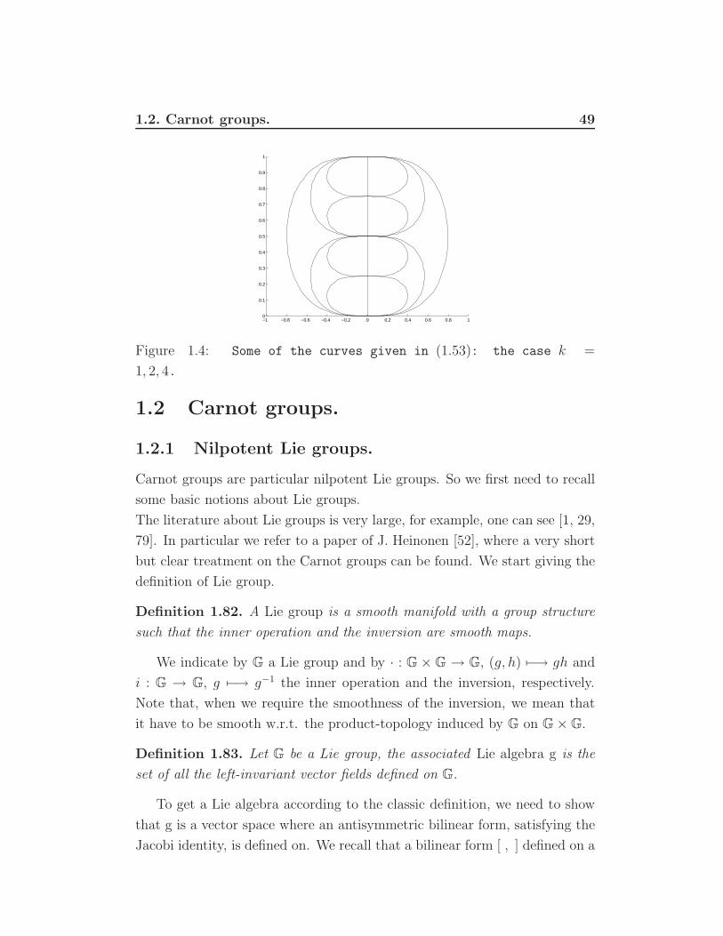
1.2. Carnot groups. 49
−1 −0.8 −0.6 −0.4 −0.2 0 0.2 0.4 0.6 0.8 10
0.1
0.2
0.3
0.4
0.5
0.6
0.7
0.8
0.9
1
Figure 1.4: Some of the curves given in (1.53): the case k =
1, 2, 4.
1.2 Carnot groups.
1.2.1 Nilpotent Lie groups.
Carnot groups are particular nilpotent Lie groups. So we first need to recall
some basic notions about Lie groups.
The literature about Lie groups is very large, for example, one can see [1, 29,
79]. In particular we refer to a paper of J. Heinonen [52], where a very short
but clear treatment on the Carnot groups can be found. We start giving the
definition of Lie group.
Definition 1.82. A Lie group is a smooth manifold with a group structure
such that the inner operation and the inversion are smooth maps.
We indicate by G a Lie group and by · : G × G → G, (g, h) 7−→ gh and
i : G → G, g 7−→ g−1 the inner operation and the inversion, respectively.
Note that, when we require the smoothness of the inversion, we mean that
it have to be smooth w.r.t. the product-topology induced by G on G × G.
Definition 1.83. Let G be a Lie group, the associated Lie algebra g is the
set of all the left-invariant vector fields defined on G.
To get a Lie algebra according to the classic definition, we need to show
that g is a vector space where an antisymmetric bilinear form, satisfying the
Jacobi identity, is defined on. We recall that a bilinear form [ , ] defined on a
50 Chapter 1. Sub-Riemannian geometries.
vector space V satisfies the Jacobi identity, if and only if, for any X, Y, Z ∈ V
the following identity holds:
[[X, Y ], Z] + [[Y, Z], X] + [[Z,X], Y ] = 0. (1.54)
Proposition 1.84. The set g of all the left-invariant vector fields (see Def-
inition 1.83) is a Lie algebra.
Proof. Let e be the unit-element of the group G, we can identify the Lie
algebra g with the tangent space at the point e, that we indicate by TeG,
associating to a vector X ∈ TeG, the left-invariant vector field Xg := LgX,
where Lg is the left translation w.r.t. the element g ∈ G. Therefore we can
see the Lie algebra g like a vector space and dim g = dim TeG = dim G.
It is trivial to check that the bracket [X, Y ] = XY − Y X defines on TeG an
antisymmetric bilinear form, which satisfies the Jacobi identity (1.54).
So we can conclude that g has the structure of a Lie algebra.
Proposition 1.85. If X ∈ g, there exists a unique 1-parameter subgroup
ΦX(t), called vector flux , defined on G, for all t ∈ R, by the system
d
dtΦX(t)
∣∣t=0
= X,
ΦX(0) = e.
Definition 1.86. Let G be a Lie group, the exponential map is the smooth
function given by
exp : g −→ G
X 7−→ ΦX(1).(1.55)
We recall some basic properties of the exponential map.
Theorem 1.87 ([91]). Let G be a Lie group and g the associated Lie algebra,
the exponential map defined by (1.55) is an analytic function. Moreover, it
is a diffeomorphism in a neighborhood of the origin.
Remark 1.88. The exponential map satisfies the following properties:
1. exp((t+ s)X
)= exp tX exp sX,
2. exp(−tX) = (exp tX)−1,
1.2. Carnot groups. 51
3. exp(X + Y ) 6= expX + exp Y .
The next result is very useful, since gives a formula in order to explicitly
compute many exponential maps.
Proposition 1.89 (Campbell-Hausdorff formula, [52]). For any X, Y ∈ g
the following formula holds:
expX exp Y = exp
(X + Y +
1
2[X, Y ] +R(X, Y )
), (1.56)
where R(X, Y ) is a remainder polynomial for a nilpotent Lie group, written
by all the possible non-vanishing k-brackets of X and Y with k ≥ 2.
Example 1.90 (Heisenberg group). The Heisenberg group is a Lie group
and the associated distribution is bracket generating with step 2.
Therefore R(X, Y ) = 0 for any X, Y ∈ g, and so formula (1.56) can be
rewritten as
expX exp Y = exp
(X + Y +
1
2XY − 1
2Y X
). (1.57)
Example 1.91 (Group of matrices). If G is a group of matrices, the expo-
nential map is the usual exponential matrix.
Definition 1.92 (Nilpotent groups). A group G is nilpotent if and only if
its central series defined as
G
(1) = G,
G(i+1) = [G,G(i)] = ghg−1h−1| g ∈ G, h ∈ G
(i), i ≥ 1,(1.58)
is finite, i.e. if and only if there exists k ∈ N such that
G(k+1) = 0 6= G
(k).
Moreover, in this case we say that G is nilpotent with step equal to k.
Remark 1.93. A group is nilpotent with step 1 if and only if it is an Abelian
group.
52 Chapter 1. Sub-Riemannian geometries.
Definition 1.94 (Nilpotent Lie algebra). A Lie algebra g is nilpotent with
step equal to k if and only if, setting
g(1) = g,
g(i+1) = [g, g(i)] = [X, Y ]|X ∈ g, Y ∈ g(i), i ≥ 1,(1.59)
there exists k ∈ N such that g(k+1) = 0 6= g(k).
Remark 1.95. Given a Lie group G, the associated Lie algebra is nilpotent
with step equal to k if and only if G is so.
Remark 1.96 (Nilpotent groups and sub-Riemannian geometries). Remark
that a Lie group is nilpotent with step k if and only if the associated Lie
algebra has a bracket generating sub-Riemannian structure with step k.
The following result is one of the main properties of the exponential map.
Proposition 1.97 ([52]). Let G be a Lie group, nilpotent and simply con-
nected, then the exponential map exp : g → G is a diffeomorphism.
Conversely, if g is a Lie algebra with finite dimension, then there exists a
unique Lie group G, simply connected, such that g is its associated Lie alge-
bra.
Remark 1.98. If G is a Lie group, nilpotent and simply connected, then it
is isomorphic to a closed unipotent subgroup of GL(n,R), where GL(n,R) is
the set of matrices with eigenvalues equal to 1. Then, there exists a system of
local coordinates where we can express it is an upper triangular matrix with
all the diagonal-elements equal to 1.
Using the Campbell-Hausdorff formula and the exponential map, we get
an easy interpretation for Lie groups.
Corollary 1.99. Let G be a Lie group, simply connected and nilpotent, then
by the exponential map we can identify G with the associated Lie algebra g
and, consequently, with Rn endowed with the polynomial operation, given by
the Campbell-Hausdorff formula, i.e. X ∗ Y := X + Y + 12[X, Y ] +R(X, Y ).
We are so able to give a geometric characterization for Abelian groups.
1.2. Carnot groups. 53
Remark 1.100. A group G is Abelian if and only if it is isomorphic to Rn
endowed with the usual (Euclidean) structure of group.
The coordinates defined by using the exponential map are usually called
canonic coordinates.
1.2.2 Calculus on Carnot groups.
In this subsection we study Carnot groups, refering to [52].
Definition 1.101 (Carnot group). A Carnot group is a Lie group, nilpotent
and simply connected, whose Lie algebra g admits a stratification, i.e. there
exist V1, ...Vk vector spaces such that
g = V1 ⊕ ...⊕ Vk.
Moreover g is endowed with the Carnot-Caratheodory metric associated to
V1.
A Lie group as in Definition 1.101 is also called homogeneous group or
stratified group. Moreover, we say that V1 generates the Lie algebra g, while
the vector spaces Vi for i ≥ 2 are called slices of g.
We now introduce a family of dilations on any Carnot group. Dilations imply
that any Carnot group is self-similar.
Definition 1.102. For λ > 0, a family of dilations on g is a family of
smooth maps δλ : g → g defined as dilations
δλ(X) = λiX, whenever X ∈ Vi. (1.60)
Applying the exponential map, we can rewritten the dilations given by
(1.60) as automorphisms of G, by setting δλ = exp−1 δλ exp. For sake of
simplicity, we still indicate δλ simply by δλ.
Note that we will indicate by dC(x, y) the Carnot-Caratheodory distance as-
sociated to a Carnot group G.
Since a Carnot-Caratheodory distance is defined minimizing the length-
functional over all the V1-horizontal curves (Definition 1.14), it follows im-
mediately that
dC(δλ(x), δλ(y)) = λdC(x, y), (1.61)
54 Chapter 1. Sub-Riemannian geometries.
for any x, y ∈ G and λ > 0.
Let G be a Carnot group and dC(x, y) the associated Carnot-Caratheodory
distance. Using the family of dilations δλ, we can define a norm on G, setting
‖x‖C := dC(0, x).
Moreover it is immediate to verify that:
‖x‖C = 0 ⇐⇒ x = 0,
‖λx‖C = dC(0, δλ(x)) = dC(δλ(0), δλ(x)) = λdC(0, x) = λ ‖x‖C .
It is possible to introduce a new norm on G equivalent to the Carnot-
Caratheodory norm ‖ ‖C but easier to compute, using the stratification-
property characterizing a Carnot group. In fact, we can write any point
x ∈ G as x = (x1, ..., xk) where xi ∈ Vi.
Definition 1.103. Let G be a Carnot group with stratification V1, ..., Vk, the
homogeneous norm is defined as
‖x‖ :=
(k∑
i=1
|xi|2k!i
) 12k!
, (1.62)
where |xi| is the usual r-dimensional Euclidean norm defined on the space
vector Vi with r = dimVi.
Example 1.104 (Homogeneous norm in the Heisenberg group). Since the
n-dimensional Heisenberg group Hn is a Carnot group with k = 2, by (1.62)
we get
‖(z, t)‖ =(|z|4 + t2
) 14 , z ∈ R
2n, t ∈ R. (1.63)
Note that
‖δλ(x)‖ = λ ‖x‖ , (1.64)
and ∥∥x−1∥∥ = ‖x‖ , (1.65)
where by x−1 we indicate the inverse element in the group G.
Using the homogeneous norm, we can define a left-invariant distance on G,
simply by taking for any x, y ∈ G
d(x, y) =∥∥x−1y
∥∥ . (1.66)
1.2. Carnot groups. 55
The function (1.66) is a distance on G and moreover it is left-invariant.
In fact, for any h ∈ G
d(hx, hy) =∥∥(hx)−1hy
∥∥ =∥∥x−1h−1hy
∥∥ =∥∥x−1y
∥∥ = d(x, y).
W.r.t. the dilations, the new distance defined in (1.66) has the same behavior
as the original Carnot-Caratheodory distance, i.e. for any x, y ∈ G
d(δλ(x), δλ(y)) = λd(x, y). (1.67)
We conclude by remarking that all the distances defined on a Carnot group
and satisfying (1.67) are equivalent.
The advantage of using the homogeneous distance instead of the Carnot-
Caratheodory distance is that the homogeneous distance is much simpler to
compute.
The main problem is that in some cases the homogeneous distance does not
satisfy a triangular inequality and so it does not induce a metric space on G.
Note that in the particular case of the Heisenberg group the homogeneous
norm (1.63) does satisfy the standard triangular inequality.
Remark 1.105 (Non-Euclidean nature of Carnot groups). There is a very
famous result by Stephen Semmes ([85]), which shows that a bi-Lipschitz
embedding of the Heisenberg group into an Euclidean space does not ex-
ist. The non-Euclidean behavior of the Carnot spaces is related to the non-
commutativity of the associated Lie algebras. In fact, if we assume that a
bi-Lipschitz emending exists, then the corresponding differential is an injec-
tive application between the two corresponding tangent spaces.
By the identification of a tangent space with the Lie algebra and using the
exponential map, we would find an isomorphism between a non-Abelian group
and an Abelian one, which gives the contradiction.

56 Chapter 1. Sub-Riemannian geometries.
1.3 The Heisenberg group.
The Heisenberg group is the most famous and the most studied sub-
Riemannian geometry.
The 1-dimensional Heisenberg algebra is the Lie algebra spanned by a
basis X, Y, Z satisfying the bracket-relations:
[X, Y ] = Z, [X,Z] = [Y, Z] = 0.
The origin of the name goes back to the fact that Heisenberg wrote down
the previous bracket-relations in his works about quantum mechanics.
x Some information on “Heisenberg’s quantum mechanics theory” can be
found in [75] (Chapter 13).
Next we give a formal definition of the n-dimensional Heisenberg group,
which is usually indicate by Hn.
Definition 1.106. Hn is the 2n + 1-dimensional Carnot group defined on
R2n+1 = Cn × R, by the following composition law
(z, t) · (z′, t′) =
(z + z′, t+ t′ +
1
2Im 〈z, z′〉
),
where Im 〈z, z′〉 is the imaginary part of the standard hermitian inner product
of Cn between z and z′.
In the next example we show that the operation defined above is non-
Abelian.
Example 1.107. Note that (1, 0, 0) · (0, 1, 0) = (1, 1, 1/2), while (0, 1, 0) ·(1, 0, 0) = (1, 1,−1/2).
The Heisenberg group is a bracket generating sub-Riemannian geometry
with step 2. Next we give two different definitions of this particular Carnot
group and we show that the two given definitions are indeed equivalent.
1.3. The Heisenberg group. 57
1.3.1 The polarized Heisenberg group.
Definition 1.108 (The polarized Heisenberg group). We call 1-dimensional
polarized Heisenberg group the sub-Riemannian geometry spanned on R3 by
the vector fields
X =
1
0
0
Y =
0
1
−x
(1.68)
endowed with the usual 2-dimensional Euclidean metric.
The bracket between X and Y gives the third dimension of the space: for
any smooth function f : R3 → R,
Zf := [X, Y ]f = X(Y f) − Y (Xf) = fxy − fz − xfxz − fyx + xfzx = −fz,
so that Z = (0, 0,−1)t.
This means that SpanX(p), Y (p), Z(p) = R3, for any p = (x, y, z) ∈ R
3,
which means that the distribution spanned by the vector fields (1.68) is
bracket generating with step 2.
Remark 1.109 ([17]). The associated sub-Riemannian metric can be written
as
ds2 = dx2 + dy2 +dz2
x2. (1.69)
By the family of dilations defined on this Carnot group, it is possible to
deduce the following estimate for the Carnot-Caratheodory.
Theorem 1.110. Let d(x, y) be the Carnot-Caratheodory distance defined
by (1.69), then for any (x, y, z) ∈ R3
1
3(|x| + |y| + |z| 12 ) ≤ d((0, 0, 0), (x, y, z)) ≤ 4(|x| + |y| + |z| 12 ). (1.70)
For a proof of the theorem see [17].
Remark 1.111. Estimate (1.70) shows that the sub-Riemannian ball cen-
tered at the origin with radius r > 0 is equivalent to the Euclidean hyper-
rectangle (−r, r) × (−r, r) × (−r2, r2).
This means that the Heisenberg geometry is an anisotropic geometry.

58 Chapter 1. Sub-Riemannian geometries.
By using the geodesic equations (1.38), we can compute the geodesics
starting from the origin. Applying (1.37), we find that the associated Hamil-
tonian is given by
H(x, y, z, p1, p2, p3) =1
2
(p2
1 + (p2 − xp3)2).
Recall that in the Heisenberg group there are not singular geodesics, the
geodesics in the polarized Heisenberg group are solutions of
x = p1
y = (p2 − xp3)
z = −x(p2 − xp3)
(1.71)
and
p1 = p3(p2 − xp3)
p2 = 0
p3 = 0
(1.72)
with initial data
x(0) = 0
y(0) = 0
z(0) = 0
p1(0) = a
p2(0) = b
p3(0) = c
(1.73)
for a, b, c ∈ R.
By (1.72) we get
p2 = b, p3 = c.
So the other equations can be rewritten as
x = p1,
y = b− cx,
z = −x(b − cx),
p1 = c(b− cx).
(1.74)
Deriving the first-equation in (1.74) and replacing that in the last equation,
we find:
x+ c2x− bc = 0. (1.75)
1.3. The Heisenberg group. 59
Assuming c 6= 0, the solutions of (1.75) with initial condition x(0) = 0 and
x(0) = p1(0) = a are
x(t) =a
csin(c t) +
b
c(1 − cos(c t)). (1.76)
From (1.76), it follows a first-order equation for the second-component of the
geodesics, more precisely
y = b− cx = b cos(c t) − a sin(c t).
By integrating with y(0) = 0, we get
y(t) =b
csin(c t) − a
c(1 − cos(c t)).
By the knowledge of x(t), we can also deduce an equation for the third-
component of the geodesics, i.e.
z = −x(b− cx) = −1
c(a sin(c t)+ b− b cos(c t))(b−a sin(c t)− b+ b cos(c t))
=a2
csin2(c t) +
b2
ccos2(c t) − ab
csin(2c t) +
ab
csin(c t) − b2
ccos(c t).
By integrating the previous equation with z(0) = 0, we find
z(t) =a2 + b2
2ct−a
2 − b2
4c2sin(2c t)+
ab
2c2cos(2c t)−ab
c2cos(c t)−b
2
c2sin(c t)+
ab
2c2.
We remain to solve the case c = 0. If c = 0 the system (1.74) can be rewritten
as
x = p1,
y = b,
z = −bx,p1 = 0.
It is easy to see that p1(t) = a and sox(t) = at,
y(t) = bt.
The third-component is deduced integrating z = −abt, i.e.
z(t) = −ab2t2.
To sum up, we have proved the following result.
60 Chapter 1. Sub-Riemannian geometries.
Theorem 1.112. The geodesics of the polarized Heisenberg group starting
from the origin are curves γ(t) = (γ1(t), γ2(t), γ3(t)) parameterized by
γ1(t) =a
csin(c t) +
b
c(1 − cos(c t)),
γ2(t) =b
csin(c t) − a
c(1 − cos(c t)),
γ3(t) =a2 + b2
2ct− a2 − b2
4c2sin(2c t) +
ab
2c2cos(2c t) − ab
c2cos(c t) − b2
c2sin(c t) +
ab
2c2,
(1.77)
for any a, b ∈ R and c 6= 0, and
γ1(t) = at,
γ2(t) = bt,
γ3(t) = −ab2t2,
(1.78)
for any a, b ∈ R.
Remark 1.113. The geodesics given in Theorem 1.112 are horizontal: in
fact γ3(t) = −γ1(t)γ2(t) for any t > 0.
1.3.2 The canonical Heisenberg group.
Definition 1.114 (Canonical Heisenberg group). We call 1-dimensional ex-
ponential Heisenberg group or also canonical Heisenberg group, the sub-
Riemannian geometry induced by the vector fields
X =
1
0
−y2
Y =
0
1x2
(1.79)
endowed with the usual 2-dimensional Euclidean metric.
Also in this case it is easy to note that the distribution is bracket
generating with step 2, since Z = [X, Y ] = (0, 0, 1)t.
Also for the canonical Heisenberg group we compute the geodesics. The
associated Hamiltonian is
H(x, y, z, p1, p2, p3) =(p1 −
y
2p3
)2
+(p2 +
x
2p3
)2
. (1.80)
1.3. The Heisenberg group. 61
The equations of the geodesics are
x = p1 −y
2p3,
y = p2 +x
2p3,
z =x
2p2 −
y
2p1 +
1
4(x2 + y2)p3,
(1.81)
and
p1 = −p3
2
(p2 +
x
2p3
),
p2 =p3
2
(p1 −
y
2p3
),
p3 = 0,
(1.82)
with initial data (1.73).
It is immediate that p3 = c, hence
p1 = −c2
(p2 +
c
2x)
= −c2y,
p2 =c
2
(p1 −
c
2y)
=c
2x.
(1.83)
By deriving (1.81) and using (1.83), we can deduce
x+ cy = 0,
y − cx = 0.(1.84)
We assume c 6= 0 and, for sake of simplicity, we set p = x and q = y.
So we have to study the first-order system
p+ cq = 0,
q − cp = 0.(1.85)
By the first-equation, we find q = −p/c, which implies q = −p/c.Replacing this in the second-equation of (1.85), we find
p+ c2p = 0. (1.86)
The solutions of (1.86) are
p(t) = k1 sin(c t) + k2 cos(c t),
62 Chapter 1. Sub-Riemannian geometries.
with k1 and k2 suitable constants. Since q = −p/c, then
q(t) = −k1 cos(c t) + k2 sin(c t).
Using the initial data (1.73), it follows that a = p1(0) = x(0) = p(0) and
b = q(0), so k1 = −b and k2 = a.
To sum up, the solutions of system (1.85) are given by
x(t) = −b sin(c t) + a cos(c t),
y(t) = b cos(c t) + a sin(c t).(1.87)
Simply integrating, we can conclude
x(t) =a
csin(c t) − b
c(1 − cos(c t)),
y(t) =b
csin(c t) +
a
c(1 − cos(c t)).
(1.88)
To find the third-component of the normal geodesics is not difficult. In fact,
by (1.88) we can write
z(t) =a2 + b2
2c(1 − cos(c t)), (1.89)
with z(0) = 0, which means
z(t) =a2 + b2
2c2(ct− sin(c t)). (1.90)
It remains only to solve (1.83) when c = 0. In this case the two first-
components are x(t) = at and y(t) = bt. So the equation for the third-
component can be written as
z = abt
2− ab
t
2= 0,
with vanishing initial condition z(0) = 0, which means z(t) = 0. Therefore
if c = 0 we have found that the usual Euclidean lines are geodesics.
In short, we have proved the following result.
1.3. The Heisenberg group. 63
Theorem 1.115. The geodesics of the canonical Heisenberg group starting
from the origin can be parameterized by
γ1(t) =a
csin(c t) − b
c(1 − cos(c t)),
γ2(t) =b
csin(c t) +
a
c(1 − cos(c t)),
γ3(t) =a2 + b2
2c2(ct− sin(c t)),
(1.91)
whenever c 6= 0, and by
γ1(t) = at,
γ2(t) = bt,
γ2(t) = 0,
(1.92)
for any a, b ∈ R.
Remark 1.116. It is immediate that all the previous curves are horizontal
and they are parameterized by arc-length whenever a2 + b2 = 1.
By the previous remark, we can give a parametrization for the unit ball in
the Heisenberg group. Looking at the geodesics parametrized by arc-length,
we can set a = cosφ and b = sinφ. The unit ball in the Heisenberg group
can be written as
x(t) =cos φ
csin(c t) − sin φ
c(1 − cos(c t)),
y(t) =sin φ
csin(c t) +
cosφ
c(1 − cos(c t)),
z(t) =ct− sin(c t)
2c2,
with 0 ≤ t < 1, 0 ≤ φ ≤ 2π and −2π ≤ c ≤ 2π.
Remark 1.117. To show Proposition 1.1, we only need to observe that the
projections of the Heisenberg geodesics (1.91) are circles, whenever they are
parameterized by arc-length (Fig. 1.6).
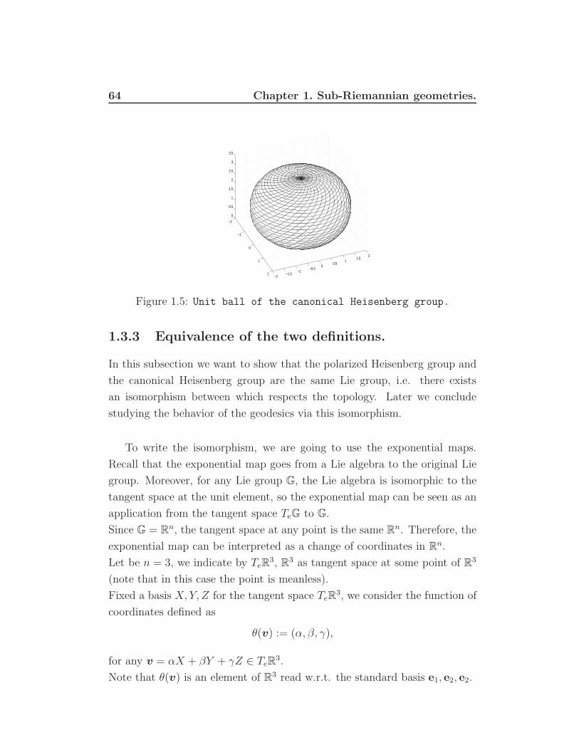
64 Chapter 1. Sub-Riemannian geometries.
−2
−1
0
1
2−2
−1.5−1
−0.50
0.51
1.52
0
0.5
1
1.5
2
2.5
3
3.5
Figure 1.5: Unit ball of the canonical Heisenberg group.
1.3.3 Equivalence of the two definitions.
In this subsection we want to show that the polarized Heisenberg group and
the canonical Heisenberg group are the same Lie group, i.e. there exists
an isomorphism between which respects the topology. Later we conclude
studying the behavior of the geodesics via this isomorphism.
To write the isomorphism, we are going to use the exponential maps.
Recall that the exponential map goes from a Lie algebra to the original Lie
group. Moreover, for any Lie group G, the Lie algebra is isomorphic to the
tangent space at the unit element, so the exponential map can be seen as an
application from the tangent space TeG to G.
Since G = Rn, the tangent space at any point is the same Rn. Therefore, the
exponential map can be interpreted as a change of coordinates in Rn.
Let be n = 3, we indicate by TeR3, R3 as tangent space at some point of R3
(note that in this case the point is meanless).
Fixed a basis X, Y, Z for the tangent space TeR3, we consider the function of
coordinates defined as
θ(v) := (α, β, γ),
for any v = αX + βY + γZ ∈ TeR3.
Note that θ(v) is an element of R3 read w.r.t. the standard basis e1, e2, e2.
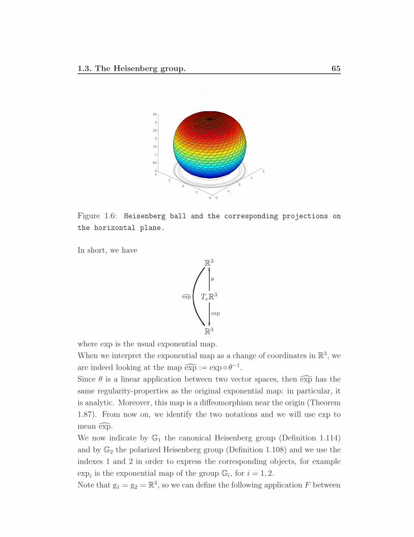
1.3. The Heisenberg group. 65
−2
−1
0
1
2
−2
−1
0
1
20
0.5
1
1.5
2
2.5
3
3.5
Figure 1.6: Heisenberg ball and the corresponding projections on
the horizontal plane.
In short, we have
R3
dexp
TeR3
exp
θ
OO
R3
where exp is the usual exponential map.
When we interpret the exponential map as a change of coordinates in R3, we
are indeed looking at the map exp := exp θ−1.
Since θ is a linear application between two vector spaces, then exp has the
same regularity-properties as the original exponential map: in particular, it
is analytic. Moreover, this map is a diffeomorphism near the origin (Theorem
1.87). From now on, we identify the two notations and we will use exp to
mean exp.
We now indicate by G1 the canonical Heisenberg group (Definition 1.114)
and by G2 the polarized Heisenberg group (Definition 1.108) and we use the
indexes 1 and 2 in order to express the corresponding objects, for example
expi is the exponential map of the group Gi, for i = 1, 2.
Note that g1 = g2 = R3, so we can define the following application F between
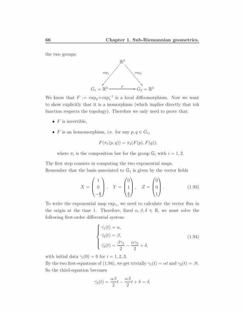
66 Chapter 1. Sub-Riemannian geometries.
the two groups:
R3
exp1
exp2
:::
::::
::::
::::
G1 = R3 F // G2 = R3
We know that F := exp2 exp−11 is a local diffeomorphism. Now we want
to show explicitly that it is a isomorphism (which implies directly that teh
function respects the topology). Therefore we only need to prove that:
• F is invertible,
• F is an homomorphism, i.e. for any p, q ∈ G1,
F (π1(p, q)) = π2(F (p), F (q)),
where πi is the composition law for the group Gi with i = 1, 2.
The first step consists in computing the two exponential maps.
Remember that the basis associated to G1 is given by the vector fields
X =
1
0
−y2
, Y =
0
1x2
, Z =
0
0
1
. (1.93)
To write the exponential map exp1, we need to calculate the vector flux in
the origin at the time 1. Therefore, fixed α, β, δ ∈ R, we must solve the
following first-order differential system:
γ1(t) = α,
γ2(t) = β,
γ3(t) =βγ1
2− αγ2
2+ δ,
(1.94)
with initial data γi(0) = 0 for i = 1, 2, 3.
By the two first-equations of (1.94), we get trivially γ1(t) = αt and γ2(t) = βt.
So the third-equation becomes
γ3(t) =αβ
2t− αβ
2t+ δ = δ.
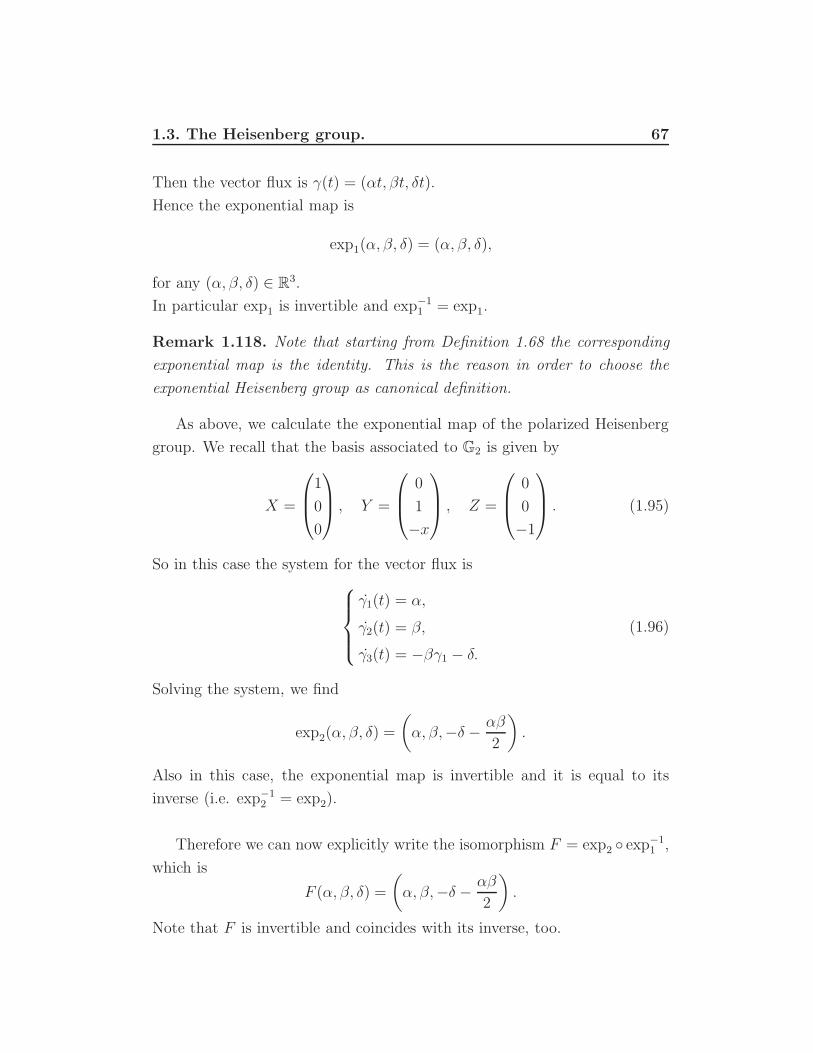
1.3. The Heisenberg group. 67
Then the vector flux is γ(t) = (αt, βt, δt).
Hence the exponential map is
exp1(α, β, δ) = (α, β, δ),
for any (α, β, δ) ∈ R3.
In particular exp1 is invertible and exp−11 = exp1.
Remark 1.118. Note that starting from Definition 1.68 the corresponding
exponential map is the identity. This is the reason in order to choose the
exponential Heisenberg group as canonical definition.
As above, we calculate the exponential map of the polarized Heisenberg
group. We recall that the basis associated to G2 is given by
X =
1
0
0
, Y =
0
1
−x
, Z =
0
0
−1
. (1.95)
So in this case the system for the vector flux is
γ1(t) = α,
γ2(t) = β,
γ3(t) = −βγ1 − δ.
(1.96)
Solving the system, we find
exp2(α, β, δ) =
(α, β,−δ − αβ
2
).
Also in this case, the exponential map is invertible and it is equal to its
inverse (i.e. exp−12 = exp2).
Therefore we can now explicitly write the isomorphism F = exp2 exp−11 ,
which is
F (α, β, δ) =
(α, β,−δ − αβ
2
).
Note that F is invertible and coincides with its inverse, too.
68 Chapter 1. Sub-Riemannian geometries.
We remain only to prove that F is an homomorphism from G1 to G2.
We need to find explicitly the two composition laws, by using the Campbell-
Hausdorff formula (1.57). First we calculate π1.
Let be p = (p1, p2, p3) and q = (q1, q2, q3), we set Xp = exp−11 p and Xq =
exp−11 q, then
Xp = p1X1 + p2Y1 + p3Z1
and analogously
Xq = q1X1 + q2Y1 + q3Z1.
Applying formula (1.57), we get
π1(p, q) = exp1Xp exp1Xq = exp1
(Xp +Xq +
1
2
[Xp, Xq
])
= exp1
(p1X1 + p2Y1 + p3Z1 + q1X1 + q2Y1 + q3Z1 +
p1q22Z1 −
p2q12Z1
)
= exp1
((p1 + q1)X1 + (p2 + q2)Y1 +
(p3 + q3 +
p1q22
− p2q12
)Z1
),
i.e.
π1(p, q) =
(p1 + q1, p2 + q2, p3 + q3 +
1
2(p1q2 − p2q1)
). (1.97)
Remark 1.119. Note that the composition law (1.97) is exactly the law given
in Definition 1.106.
To find the composition law of G2, we start from Xp = exp−12 p and
Xq = exp−12 q, which gives
Xp = p1X2 + p2Y2 +(−p3 −
p1p2
2
)Z2
and
Xq = q1X2 + q2Y2 +(−q3 −
q1q22
)Z2.
In this case, formula (1.57) gives
π2(p, q) = exp2 Xp exp2 Xq = exp2
(Xp + Xq +
1
2
[Xp,Xq
])= exp2
(p1X2+p2Y2
+
(−p3 −
p1p2
2
)Z2 + q1X2 + q2Y2 +
(−q3 −
q1q2
2
)Z2 +
p1q2
2Z2 −
p2q1
2Z2
)
= exp2
((p1 + q1)X2 + (p2 + q2)Y2 +
(−p3 −
p1p2
2− q3 −
q1q2
2+
p1q2
2− p2q1
2
)Z2
)
=
(p1 + q1, p2 + q2, p3 + q3 +
p1p2
2+
q1q2
2− p1q2
2+
p2q1
2− 1
2(p1 + q1)(p2 + q2)
).
1.3. The Heisenberg group. 69
Hence
π2(p, q) = (p1 + q1, p2 + q2, p3 + q3 − p1q2). (1.98)
By (1.97) and (1.98), it is easy to check that F is an homomorphism between
G1 and G2, in fact:
F(π1(p, q)
)= F
(p1 + q1, p2 + q2, p3 + q3 +
1
2(p1q2 − p2q1)
)
=
(p1 + q1, p2 + q2,−p3 − q3 −
1
2(p1q2 − p2q1) −
1
2(p1 + q1)(p2 + q2)
)
=(p1 + q1, p2 + q2,−p3 − q3 −
p1p2
2− q1q2
2− p1q2
).
On the other side,
π2
(F (p), F (q)
)= π2
((p1, p2,−p3 −
p1p2
2
),(q1, q2,−q3 −
q1q22
))
=(p1 + q1, p2 + q2,−p3 − q3 −
p1p2
2− q1q2
2− p1q2
).
Therefore
F(π1(p, q)
)= π2
(F (p), F (q)
)
and so F is the isomorphism between G1 and G2 which we are looking for.
We conclude showing that, by the application of F , the geodesics (1.91)
go into the geodesics (1.76) and, analogously, the geodesics (1.92) goes into
the geodesics (1.78).
It is immediate to note that F fixes the first-component and the second-
component of any curve. Nevertheless the two first-components of the cor-
responding geodesics are not the same. In fact, the parameter c depends on
the orientation of the vector field Z. So, if we want to compute the range
of geodesics associated to the same parameters, we must start by geodesic-
equations (1.91), rewritten w.r.t. −c, i.e.
γ(t) =
γ1(t) =a
csin ct+
b
c(1 − cos ct),
γ2(t) =b
csin ct− a
c(1 − cos ct),
γ3(t) = −a2 + b2
2c2(ct− sin ct).
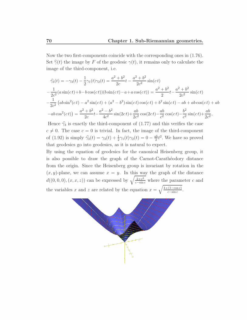
70 Chapter 1. Sub-Riemannian geometries.
Now the two first-components coincide with the corresponding ones in (1.76).
Set γ(t) the image by F of the geodesic γ(t), it remains only to calculate the
image of the third-component, i.e.
γ3(t) = −γ3(t) −1
2γ1(t)γ2(t) =
a2 + b2
2ct − a2 + b2
2c2sin(c t)
− 1
2c2(a sin(c t)+b−b cos(c t))(b sin(c t)−a+a cos(c t)) =
a2 + b2
2t− a2 + b2
2c2sin(c t)
− 1
2c2
(ab sin2(c t) − a2 sin(c t) + (a2 − b2) sin(c t) cos(c t) + b2 sin(c t) − ab + ab cos(c t) + ab
−ab cos2(c t))
=a2 + b2
2ct−a2 − b2
4c2sin(2c t)+
ab
2c2cos(2c t)−ab
c2cos(c t)−b2
c2sin(c t)+
ab
2c2,
Hence γ3 is exactly the third-component of (1.77) and this verifies the case
c 6= 0. The case c = 0 is trivial. In fact, the image of the third-component
of (1.92) is simply γ3(t) = γ3(t) + 12γ1(t)γ2(t) = 0 − ab
2t2. We have so proved
that geodesics go into geodesics, as it is natural to expect.
By using the equation of geodesics for the canonical Heisenberg group, it
is also possible to draw the graph of the Carnot-Caratheodory distance
from the origin. Since the Heisenberg group is invariant by rotation in the
(x, y)-plane, we can assume x = y. In this way the graph of the distance
d((0, 0, 0), (x, x, z)) can be expressed by√
2 z c2
c−sin cwhere the parameter c and
the variables x and z are related by the equation x =√
4 z (1−cos c)c−sin c
.
Chapter 2
Viscosity solutions and metric
Hopf-Lax formula.
2.1 An introduction to the theory of viscosity
solutions.
Let us start by a simple example: the 1-dimensional eikonal equation. We
consider the following Dirichlet problem:
|u′(x)| = 1, x ∈ (−1, 1),
u(−1) = u(1) = 0.(2.1)
It is easy to note that there are not classical solutions for Dirichlet problem
(2.1). In fact, given a function u ∈ C1([−1, 1]) such that u(−1) = u(1) = 0,
by Rolle’s Theorem there exists a point x0 ∈ (−1, 1) such that
u′(x0) =u(1) − u(−1)
2= 0.
So the euquation is not satisfied at the point x0. Moreover by continuity of
u′(x), |u′(x)| < 1 in some open neighborhood of x0. The condition u ∈ C1 is
clearly too strong to get general existence results for nonlinear PDEs.
Therefore the idea of looking at weaker notions of solutions for nonlinear
PDEs as the eikonal equation.
For example, if we look at the function u(x) = −|x|+ 1 (which is continuous
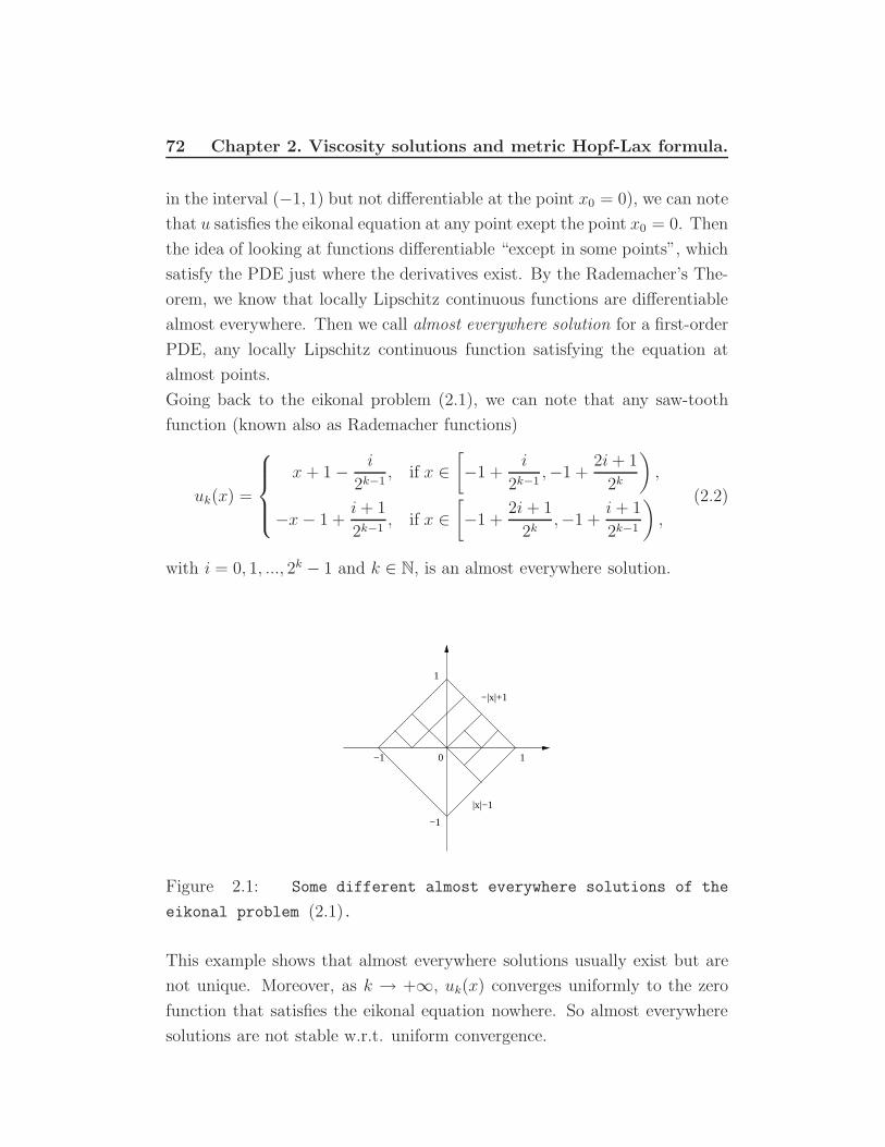
72 Chapter 2. Viscosity solutions and metric Hopf-Lax formula.
in the interval (−1, 1) but not differentiable at the point x0 = 0), we can note
that u satisfies the eikonal equation at any point exept the point x0 = 0. Then
the idea of looking at functions differentiable “except in some points”, which
satisfy the PDE just where the derivatives exist. By the Rademacher’s The-
orem, we know that locally Lipschitz continuous functions are differentiable
almost everywhere. Then we call almost everywhere solution for a first-order
PDE, any locally Lipschitz continuous function satisfying the equation at
almost points.
Going back to the eikonal problem (2.1), we can note that any saw-tooth
function (known also as Rademacher functions)
uk(x) =
x+ 1 − i
2k−1, if x ∈
[−1 +
i
2k−1,−1 +
2i+ 1
2k
),
−x− 1 +i+ 1
2k−1, if x ∈
[−1 +
2i+ 1
2k,−1 +
i+ 1
2k−1
),
(2.2)
with i = 0, 1, ..., 2k − 1 and k ∈ N, is an almost everywhere solution.
−1 1
1
−1
0
−|x|+1
|x|−1
Figure 2.1: Some different almost everywhere solutions of the
eikonal problem (2.1).
This example shows that almost everywhere solutions usually exist but are
not unique. Moreover, as k → +∞, uk(x) converges uniformly to the zero
function that satisfies the eikonal equation nowhere. So almost everywhere
solutions are not stable w.r.t. uniform convergence.
2.1. An introduction to the theory of viscosity solutions. 73
We are going to introduce a different notion of weak solutions which leads
to existence, uniqueness and stability for a large class of nonlinear PDEs:
the so called viscosity solutions.
Viscosity solutions for Hamilton-Jacobi first-order PDEs have been intro-
duced in the early ’80 by M.G. Crandall and P.L. Lions in [39] (see [40] for
the English version). In the following years, many authors have been worked
to develop this new theory, hence many results for existence, uniqueness
and regularity for first-order and second-order nonlinear PDEs have been
proved. Here we will concentrate in particular on first-order equations, for
more datails on the second-order case, we suggest to look at [23, 38].
2.1.1 Viscosity solutions for continuous functions.
We now introduce the classical theory of viscosity solutions for continuous
functions. This theory has been introduced by M.G. Crandall and P.L. Lions
in [39, 40] and then developed by H. Ishii, G. Barles, L.C. Evans and many
others. In particular, we suggest to see [7, 11, 47, 71] for a very useful and
clear treatment of viscosity theory for the Hamilton-Jacobi equations.
We begin giving the main definitions.
Definition 2.1. Let Ω ⊂ Rn be an open set and u : Ω → R a continuous
function and let us consider the first-order PDE
H(x, u(x), Du(x)) = 0, x ∈ Ω. (2.3)
(i) We say that u is a viscosity subsolution of (2.3) at a point x0 ∈ Ω if
and only if for any test function ϕ ∈ C1(Ω) such that u−ϕ has a local
maximum at x0, then
H(x0, u(x0), Dϕ(x0)) ≤ 0; (2.4)
(ii) We say that u is a viscosity supersolution of (2.3) at a point x0 ∈ Ω,
if and only if, for any test function ϕ ∈ C1(Ω) such that u − ϕ has a
local minimum at x0, then
H(x0, u(x0), Dϕ(x0)) ≥ 0; (2.5)

74 Chapter 2. Viscosity solutions and metric Hopf-Lax formula.
(iii) We say that u is a viscosity solution in the open set Ω if u is a viscosity
subsolution and a viscosity supersolution at any point x0 ∈ Ω.
Remark 2.2. An analogous definition holds for second-order PDEs.
Remark 2.3. If u(x) − ϕ(x) has a local maximum (resp. minimum) at x0,
we can assume that the maximum (resp. minimum) is zero and moreover, by
adding a suitable quadratic perturbation, we can suppose that the maximum
(resp. minimum) is strict (see [36], Lemma 1.1).
Example 2.4. We want to show that u(x) = |x| is the unique viscosity
solution of the eikonal equation
−|Du(x)| + 1 = 0, x ∈ (−1, 1). (2.6)
For the uniqueness see [7].
Note that, whenever x0 6= 0, x0 is an extremal-point for u − ϕ where the
function is differentiable, then D(ϕ− u)(x0) = 0, which means
Dϕ(x0) = Du(x0) = 1.
The problem occurs only at the point x0 = 0, where the modulus is not
differentiable. Let us first consider the subsolution property, i.e. x0 local
(strict) maximum point and assume u(0) = ϕ(0); then −|x| ≤ u(x)− u(0) ≤ϕ(x) − ϕ(0), near 0, which implies
1 ≥ ϕ(x) − ϕ(0)
x, for x < 0 and
ϕ(x) − ϕ(0)
x≥ −1, for x > 0.
Since ϕ ∈ C1, passing to the limit as x → 0, we can conclude |ϕ′(0)| ≤1. Therefore the subsolution condition (2.4) is satisfied at any point x0 ∈(−1, 1). To verify the supersolution condition, we assume that u−ϕ attends
a local maximum (equal to 0) at the point 0. Proceeding as above we find
D−ϕ(0) ≥ 1 and D+ϕ(0) ≤ −1, which means D−ϕ(0) 6= D+ϕ(0). Therefore
there cannot be C1-functions touching u(x) = −|x| + 1 from below, which
means the condition (2.5) is trivially verified.
Example 2.5. Similarly to the previous example, one can show that v(x) =
−u(x) = −|x| is a viscosity solution of
|Du(x)| − 1 = 0, x ∈ (−1, 1). (2.7)
2.1. An introduction to the theory of viscosity solutions. 75
Remark 2.6. Note that while u(x) = |x| does not satisfy Eq. (2.7) in the
viscosity sense. In fact, the function ϕ(x) = −x2+1 is a C1 function touching
u from above at 0. Nevertheless −|ϕ′(0)|+1 = 1 > 0, therefore the subsolution
property is not satisfied.
In fact, the equations H(x, u,Du) = 0 and −H(x, u,Du) = 0 are not in
general equivalent in the viscosity sense. It is very easy to show that, if u(x)
is a viscosity solution of H(x, u,Du) = 0, then v(x) = −u(x) is a viscosity
solution of −H(x,−v,−Dv) = 0.
In the next propositions we show that the definition of viscosity solutions
is consistent with the notion of classical solutions: in fact classical solutions
are viscosity solutions, too, and C1-viscosity solutions are also classic solu-
tions.
Proposition 2.7. Let Ω be an open set and u ∈ C1(Ω). Then u is a viscosity
solution if and only if u is a classical solution.
Proof. To prove that C1-viscosity solutions are also classical solutions is triv-
ial. In fact, we can choose, as test function, u itself and, therefore, it satisfies
the equation in the classical sense.
In order to get the inverse implication, we can observe that, for any test
function ϕ, if x0 is an extremal point of u − ϕ where both of the functions
are differentiable, then Du(x0) = Dϕ(x0). So if u satisfies the equation, any
test function does so and, therefore, u is a viscosity solution.
Remark 2.8. For second-order PDEs the consistence with classical solutions
is not always true. In this case, one has to assume that the equation is non-
increasing in the second-order variables (e.g. elliptic or degenerate elliptic
PDEs). Moreover, to ensure uniqueness at least of classical solutions, usually
we assume also a monotone-increasing dependence w.r.t. u.
The previous proposition can be written punctually, as follows.
Remark 2.9. If u is a viscosity solution at a point where it is differentiable,
then u satisfies the equation in the classical sense at that point (see [47],
Theorem 10.1.1 for a proof of this result).
76 Chapter 2. Viscosity solutions and metric Hopf-Lax formula.
Viscosity solutions are also consistent with almost everywhere solutions,
in the sense that any locally Lipschitz continuous viscosity solution satisfies
the PDE almost everywhere.
Proposition 2.10. Let Ω be an open set and u be a viscosity solution in Ω.
If u is Lipschitz in Ω (briefly u ∈ Lip(Ω)), then u is an almost everywhere
solution, too.
Proof. The result follows immediately by Remark 2.9 and the Rademacher’s
Theorem.
Remark 2.11. The reverse implication of Proposition 2.10 is in general not
true, as we have seen in the case of the eikonal equation.
Now we want to investigate the stability properties for viscosity solutions.
Proposition 2.12. Let Ω be an open set and u ∈ C(Ω) and suppose x0 is a
maximum point (resp. minimum point) for u − ϕ in Br(x0) ⊂ Ω, for some
ϕ ∈ C1(Ω). If un ∈ C(Ω) are such that
limn→∞
un(x) = u(x),
for any x ∈ Ω, let xn be a sequence of minimum points for un −ϕ in Br(x0),
then xn → x, as n→ ∞, and moreover
limn→∞
un(xn) = u(x0).
From the previous result the stability follows imediately.
Proposition 2.13. Let Hn and H be continuous in all the variables and such
that Hn → H, as n→ ∞. Let un be viscosity solutions of Hn(x, un, Dun) = 0
and
u(x) = limn→+∞
un(x).
If u is continuous, then u is a viscosity solution of H(x, u,Du) = 0.
The proofs of the two previous results are here omitted and we will give
those later directly in the semicontinuous case (see Proposition 2.23 and
Proposition 2.25).
2.1. An introduction to the theory of viscosity solutions. 77
Another important property of viscosity solutions is the behavior w.r.t.
the operations of infimum and supremum. Let us start by the easy case of
only two (or a finite number of) continuous functions.
Proposition 2.14.
1. Let u, v ∈ C(Ω) be two viscosity subsolutions of H(x, u,Du) = 0, then
u ∨ v is a viscosity subsolution of the same equation.
2. Let u, v ∈ C(Ω) be two viscosity supersolutions of H(x, u,Du) = 0,
then u ∧ v is a viscosity supersolution of the same equation.
The proof of the previous result is pretty easy (e.g. [7], Proposition 2.1).
The previous result can be generalized to inifinitly many functions.
Proposition 2.15.
1. Let F be a family of viscosity subsolutions of H(x, u,Du) = 0,
and define
u(x) := supv∈F
v(x).
If u is continuous, then u is a viscosity subsolution of the equation.
2. Let F be a family of viscosity supersolutions of H(x, v,Dv) = 0,
and define
u(x) := infv∈F
v(x).
If u is continuous, then it is a viscosity supersolutions of the same
equation.
We now omit the proof since we are going to give that directly for lower
semicontinuous viscosity solutions (see Proposition 2.26).
The behavior w.r.t. to the infimum (and the supremum respectively) is the
key point to get existence of viscosity solutions by the so called Perron’s
method [81]. In 1987 H. Ishii used for the first time the Perron’s method to
solve nonlinear first-order equations (Perron’s method for Hamilton-Jacobi
equations, Duke Math. J. 55). This method had been introduced in 1923
by Oskar Perron in order to find solutions for the Laplace equation and con-
sists in building a solution as the supremum of a suitable family of viscosity
78 Chapter 2. Viscosity solutions and metric Hopf-Lax formula.
subsolutions. Since the supremum of viscosity subsolutions is a viscosity sub-
solution, one has just to prove that it is a viscosity supersolution, too.
The Perron’s method can be sketched, as follows:
Theorem 2.16 (Perron’s Method). Let us assume that
1. Comparison principle for the equation holds, i.e. given u viscosity sub-
solution and v viscosity supersolution satisfying the same boundary con-
dition, then u ≤ v.
2. Suppose that there exist u and u which are, respectively, a viscosity
subsolution and a viscosity supersolution, satisfying the same boundary
condition.
We define
W (x) = supw(x) | u ≤ w ≤ u and w viscosity subsolution,
Then W (x) is a viscosity solution of the same equation, which satisfies the
same boundary condition satisfied by u and u.
The Perron’s method is one of the most used method in order to get
existence of solutions in the classical sense as well as in the viscosity sense.
However we quote the result without giving any proof since we will apply
a different method to prove existence for our class of PDEs, by the use of
a suitable representative formula, the so called Hopf-Lax function (we will
give many datails on this formula in Sec. 2.3).
Another method to get existence for nonlinear PDEs is the so called method
of the characteristics. We refer to [47] for more details on this method.
A last method for existence of viscosity solution we like to quote is the so
called vanishing viscosity approximation, which consists in adding to the
equation a “viscosity term”, i.e. a term of the form −ε∆u, for any ε > 0.
This leads often to an elliptic or parabolic PDE, which is usually easier to
solve than the starting Hamilton-Jacobi equation. Several times it is even
possible to get classical solutions for the family of approximating PDEs.
The limit of those classical solutions solves in the viscosity sense the starting
Hamilton-Jacobi equation. The name “viscosity solutions” comes exactly

2.1. An introduction to the theory of viscosity solutions. 79
from this idea. We will go back on the vanishing viscosity approximation in
the last section. More information can be found in [71] (Sec. 1.4 and Sec.
8), [47] (Sec. II.7.3), [36] (Theorem 3.1.) or [13, 87, 40]. See also [9] for a
similar method.
We conclude quoting some results conerning uniqueness. Whenever the
Hamiltonian satisfies some a coercive assumption or a Lipschitz assumption
w.r.t. the gradient-variable, uniqueness for the the Dirichlet problem or
the Cauchy problem can be found in [7, 11, 37, 41, 47, 71] and, only for
the evolution equation, in [36, 58], too. In particular, we like to quote a
pretty recent by A. Cutrı and G. Da Lio ([42]), which holds for the Cauchy
problem and Hamiltonians satisfying a very general Hormander condition
(which means for the kind of degenerate Hamiltonians we are going to treat
in this Thesis, see Sec. 2.4.2).
2.1.2 Discontinuous viscosity solutions.
There are different ways to define a notation of viscosity solutions, for discon-
tinuous functions. By Weirstrass Theorem, we know that in Rn any contin-
uous function attends maximum and minimum in a closed ball. This means
that it is sufficient to require lower semicontinuity for viscosity supersolution
(where we test at minimum points) and upper semicontinuous for viscosity
subsolutions (where instead we test at maximum points). If the function is
not continuous we can consider the right semicontinuous regularization of
the function to test the supersolution and subsolution conditions. This leads
to the following notion.
Definition 2.17. Let Ω ⊂ Rn be an open set and u : Ω → R be locally
bounded function.
1. We say that u is a (discontinuous) viscosity subsolution of
H(x, u,Du) = 0 if, defined the upper semicontinuous envelop of u
u∗(x) := infv(x)|v ∈ C(Ω) and v ≥ u in Ω = lim supr→0+
u(y)| |y−x| ≤ r,
u∗ is a viscosity subsolution of the equation.
80 Chapter 2. Viscosity solutions and metric Hopf-Lax formula.
2. We say that u is a (discontinuous) viscosity supersolution of
H(x, u,Du) = 0 if, defined the lower semicontinuous envelop of u
u∗(x) := supv(x)|v ∈ C(Ω) and v ≤ u in Ω = lim infr→0+
u(y)| |y−x| ≤ r,
u∗ is a viscosity supersolution of the equation.
3. We say that u is a (discontinuous) viscosity solution of H(x, u,Du) = 0
if u∗ is a viscosity subsolution of the equation and u∗ is a viscosity
supersolution of the equation.
Remark 2.18. Note that u∗ and u∗ are locally bounded and upper and lower
semicontinuous, respectively. Moreover u∗ ≤ u ≤ u∗.
This notion of discontinuous viscosity solutions is used in [57, 56, 12]
to get existence and uniqueness for a pretty large class of Hamilton-Jacobi
equations.
In this thesis we istead follow a different notion of discontinuous viscosity
solutions, which has been introduced by Barron and Jensen in [14, 15] and
then applied to Dirichlet problem by Barles in [10] and to the Cauchy problem
for bounded equations in infinite-dimensional spaces by Ishii in [59]. Some
objections concerning the use of upper and lower semicontinuous envelopes
to solve problems with discontinuous initial data can be found in [14]. We
only remark that we are going to look at lower semicontinuous initial data.
The easiest idea is so to apply directly the standard definition but testing
only at the minimum points. For Hamiltonian which are convex w.r.t. the
gradient, there is a very consistent way to do this. Let us give more details.
Definition 2.19. Let Ω be an open set and u be a lower semicontinuous
(briefly u ∈ LSC(Ω)), we say that u is a lower semicontinuous viscosity
solution (shorthly LSC-viscosity solutions) for Eq. (2.3) at some point x0 ∈ Ω
if and only if for any test function ϕ ∈ C1(Ω) such that u−ϕ attends a local
minimum at x0, then
H(x0, ϕ(x0), Dϕ(x0)) = 0. (2.8)
Remark 2.20. Note that Definition 2.19 differs from the standard viscosity
supersolution requirement because of the identity instead of the inequality.

2.1. An introduction to the theory of viscosity solutions. 81
Therefore Definition 2.19 is also called strong viscosity supersolution condi-
tion.
LSC-viscosity solutions satisfy almost all of the properties that we have
seen for continuous viscosity solutions. Moreover Definition 2.19 is consistent
with the standard definition of viscosity solutions (Definition 2.1).
A very nice proof of this result can be found in [10] (Theorem 2.1).
In [14] the authors have proved the consistence for evolution Hamitlon-Jacobi
equations of the form
ut(t, x) +H(x, u,Du) = 0, (2.9)
where by Du we indicate the gradient w.r.t. x, by assumeing that the Hamil-
tonian is Lipschitz w.r.t. the gradient. We will show that this assumption is
indeed not necessary for the consistence.
Theorem 2.21. Let be Ω = [0,+∞) × Rn and let H(x, z, p) = H(x, p) be
continuous in both of the variables and convex w.r.t. p. We assume that for
R > 0 there exists a family of modulus of continuity ωR(·) and a continuous
function f : [0,+∞) → [0,+∞) such that
|H(x, p) −H(y, p)| ≤ ωR(|x− y|)f(|p|) ∀x, y ∈ BR(0). (2.10)
Then, if u ∈ C(Ω) is a LSC-viscosity solution of Eq. (2.9), then u is a
standard viscosity solution (Definition 2.1).
Proof. It is immediate that if u ∈ C(Ω) is a strong viscosity supersolution
(i.e. Definition 2.19 holds) then u is in particular a viscosity supersolution.
So we need only to check that it is a viscosity subsolution, too, by using the
convexity of H w.r.t. the gradient.
So let ϕ ∈ C1(Ω) be such that u−ϕ attends a local maximum at (t0, x0), we
have to prove that
ϕt(t0, x0) +H(x0, Dϕ(t0, x0)) ≤ 0. (2.11)
Define φ = u − ϕ, we apply Theorem 1.1 in [14]: for any ε > 0 there exist
ψ ∈ C∞(Ω), αk and (tk, xk), with k = 1, ..., N < +∞, such that
82 Chapter 2. Viscosity solutions and metric Hopf-Lax formula.
(i) αk ≥ 0, for any k = 1, ..., N and∑N
k=1 αk = 1,
(ii) φ−ψ attends a minimum equal to 0 at any point (tk, xk), for k = 1, ..., N .
(iii) (tk, xk) ∈ Boε(1)ε1/2(s, y) for some (s, y) ∈ Boε(1)(t0, x0), where by oε(1)
we indicate a quantity going to 0 as ε → 0+.
(iv)∑N
k=1 αkψt(tk, xk) = 0 =∑N
k=1 αkDψ(tk, xk).
Since (tk, xk) are minimum points for u−ϕ−ψ and u satisfies the equation,
then ϕ = ϕ+ ψ is a test function touching from above at (tk, xk), hence
ϕt(tk, xk)+ψt(tk, xk)+H(xk, Dϕ(tk, xk)+Dψ(tk, xk)) = 0, for any k = 1, .., N.
We add and subtract ±ϕt(s, y), ±H(y,Dϕ(tk, xk)) and ±H(y,Dϕ(s, y) +
Dψ(tk, xk)), and we estimate the corresponding differences. By property
(iii) and using that ϕ ∈ C1(Ω), we get
ϕt(tk, xk) − ϕt(s, y) ≥ −oε(1)ε12 = −oε(1).
Moreover
|H(xk, Dϕ(tk, xk)) −H(y,Dϕ(tk, xk))| ≤ ω(|xk − y|)f(|Dϕ(tk, xk)|).
By property (iii) we know that (tk, xk) ∈ Boε(1)(s, y) and (s, y) ∈Boε(1)(t0, x0); hence (tk, xk) ∈ K compact subset of [0,+∞) × Rn for any
k = 1, ..., N . Since f and Dϕ are continuous, then f(|Dϕ(tk, xk)|) ≤ C for
any k = 1, ..., N , which implies
|H(xk, Dϕ(tk, xk)) −H(y,Dϕ(tk, xk))| ≤ Cω(|xk − y|) = oε(1).
We remain to estimate the last term, using the convexity ofH(x, p) w.r.t. the
gradient which implies that the Hamiltonian is locally Lipschitz continuous
w.r.t. the gradient. Note that (tk, xk), (s, y) ∈ Br(t0, x0), so by the local
Lipschitz continuity of H , we find
|H(y,Dϕ(tk, xk) +Dψ(tk, xk) −H(y,Dϕ(s, y) +Dψ(tk, xk)|≤ C|Dϕ(tx, xk) −Dϕ(s, y)| = oε(1).
2.1. An introduction to the theory of viscosity solutions. 83
To sum up, we have found the following estimate
oε(1) ≥ ϕt(s, y) + ψt(tk, xk) +H(y,Dϕ(s, y) +Dψ(tk, xk)).
Multiplying by αk ≥ 0 and summing over k = 1, ..., N , we can use the
convexity of H w.r.t. p, so that
N∑
k=1
αkoε(1) ≥N∑
k=1
αkϕt(s, y) +
N∑
k=1
αkψt(tk, xk)
+H
(y,
N∑
k=1
αkDϕ(s, y) +
N∑
k=1
αkDψ(tk, xk)
).
Using property (iv), we get
oε(1) ≥ ϕt(s, y) +H(y,Dϕ(s, y));
using that ϕ ∈ C1(Ω) and (s, y) ∈ Boε(1)(t0, x0), passing to the limit as
ε → 0+, we find (2.11).
Remark 2.22. The Hamiltonian H(x, p) = 1α|σ(x)p|α for α ≥ 1 satisfies all
the assumptions of Theorem 2.21 hold whenever σ(x) has smooth coefficients.
We now show some properties for LSC-viscosity solutions.
Proposition 2.23. Let u be a lower semicontinuous function, ϕ ∈ C1 and
x0 a minimum point for u − ϕ in Br(x0). Let un be a sequence of lower
semicontinuous functions such that
lim infn→∞
un(x) = u(x).
If xn is a sequence of minimum points for un −ϕ in Br(x0), then xn → x as
n→ ∞ and moreover
lim infn→∞
un(xn) = u(x0).
Proof. Without loss of generality, we can assume that the minimum in Br(x0)
is strict. Moreover Br(x0) is a compact set and so there exists a subsequence
of xn (which we still indicate by xn) which converges to some point y ∈

84 Chapter 2. Viscosity solutions and metric Hopf-Lax formula.
Br(x0).
We need only to check that y = x0. Note that
un(xn) − ϕ(xn) ≤ un(x) − ϕ(x), ∀x ∈ Br(x0).
Since un is lower semicontinuous for any n ∈ N and xn → y, passing to the
lower limit in the previous inequality, we find
u(y) − ϕ(y) ≤ lim infn→+∞
un(xn) − ϕ(y) ≤ u(x) − ϕ(x). (2.12)
Therefore y is a minimum point for u−ϕ in Br(x0). Since we have assumed
that the minimum is strict, then y = x0.
Moreover, writing (2.12) at the point x = x0, we get
u(x0) − ϕ(x0) ≤ lim infn→+∞
un(xn) − ϕ(x0) ≤ u(x0) − ϕ(x0).
We can so conclude that
lim infn→+∞
un(xn) = u(x0).
Remark 2.24. Without loss of generality we can assume un(xn) = ϕ(xn)
for any n, which implies u(x0) = ϕ(x0).
The previous lemma can be used to show the stability of LSC-viscosity
solutions.
Proposition 2.25. Let Hn(x, z, p) and H(x, z, p) be continuous Hamiltoni-
ans and assume that Hn(x, z, p) → H(x, z, p) as n → ∞. Let un be LSC-
viscosity solutions of Hn(x, un, Dun) = 0. Define
u(x) = lim infn→+∞
un(x).
If u is a lower semicontinuous function, then u is a LSC-viscosity solution
for the limit-equation H(x, u,Du) = 0.
Proof. Let ϕ ∈ C1 be such that u− ϕ attends a local strict minimum at x0,
which means there exists r > 0 such that
u(x0) − ϕ(x0) < u(x) − ϕ(x), ∀x ∈ Br(x0)\x0.
2.1. An introduction to the theory of viscosity solutions. 85
Since un are lower semicontinuous functions, there is a sequence of points xn
where un − ϕ attends minimum in Br(x0).
By Proposition 2.23 xn → x0; hence there exists n ∈ N such that for any
n > n, xn ∈ Br(x0) and
lim infn→+∞
un(xn) = u(x0).
We recall that ϕ(xn) = un(xn) and ϕ(x0) = u(x0) (see Remark 2.24): un are
LSC-viscosity solutions of Hn(x, un, Dun) = 0, so
Hn(xn, ϕ(xn), Dϕ(xn)) = 0.
Moreover ϕ ∈ C1 and H(x, z, p) continuous; hence passing to the limit as
n→ ∞, we get
H(x, ϕ(x0), Dϕ(x0)) = 0.
Next we study the behavior of LSC-viscosity solutions w.r.t. the infimum
and the supremum.
Proposition 2.26. Let v ∈ F be a family of LSC-viscosity solutions of
H(x, v,Dv) = 0 and u(x) = infv∈F v(x). If u is a lower semicontinuous
function, then it is a LSC-viscosity solution of the same equation.
Proof. Let ϕ ∈ C1 be such that u− ϕ has a local strict minimum at x0, i.e.
there exists r > 0 such that
u(x0) − ϕ(x0) < u(x) − ϕ(x), ∀x ∈ Br(x0)\x0.
Since u(x0) = infv(x0) | v ∈ F, for any n ∈ N there exists vn ∈ F such
that
vn(x0) < u(x0) +1
n.
Let xn be a sequence of minimum points for vn − ϕ in Br(x0), i.e.
vn(xn) − ϕ(xn) ≤ vn(x) − ϕ(x), ∀x ∈ Br(x0), (2.13)

86 Chapter 2. Viscosity solutions and metric Hopf-Lax formula.
we know that (up to a subsequence) xn → y for some point y ∈ Br(x0).
Writing (2.13) at the point x = x0, we find
u(xn) − ϕ(xn) ≤ vn(xn) − ϕ(xn) ≤ vn(x0) − ϕ(x0) < u(x0) +1
n− ϕ(x0).
Passing to the lower limit as n → +∞, and using the lower semicontinuity
of u and the continuity of test function ϕ, we conclude
u(y) − ϕ(y) ≤ u(x0) − ϕ(x0).
Therefore y is a minimum point of u− ϕ in Br(x0). Since x0 is a strict pint
of minimum, then x0 = y.
We now use that vn are LSC-viscosity solutions (with ϕ(xn) = un(xn)), i.e.
H(xn, ϕ(xn), Dϕ(xn)) = 0.
Passing to the limit as n→ +∞ and, recalling that ϕ(x0) = u(x0), we find
H(x0, u(x0), Dϕ(x0)) = 0.
We are going to look in particular at the Cauchy problem for an evolution
Hamilton-Jacobi equation:
ut +H(t, x, u,Du) = 0, in R
n × (0,+∞),
u = g, in Rn × 0,
(2.14)
with a lower semicontinuous initial data g.
For sake of simplicity, we prefer to re-write Definition 2.19 explicitly in the
evolution case
Definition 2.27. Let Ω be an open subset of Rn×(0,+∞) and u ∈ LSC(Ω),
u is a LSC-viscosity solution for the Hamilton-Jacobi equation (2.9), at the
point (t0, x0) if and only if, for any test function ϕ ∈ C1(Ω) such that u− ϕ
attends a local minimum at (t0, x0),
∂ϕ
∂t(t0, x0) +H(t0, x0, u(t0, x0), Dϕ(t0, x0)) = 0. (2.15)
2.2. The generalized eikonal equation. 87
In [14] the authors have proved that upper semicontinuous viscosity solu-
tions (defined testing the subsolution-property at the maximum points) for
a terminal-time Cauchy problem are unique, under suitable assumptions on
the Hamiltonians. In particular the Hamiltonian is assumed to be globally
Lipschitz w.r.t. the gradient. By this result, the uniqueness for LSC-viscosity
solutions of (2.14) follows immediately.
We like to quote also [10], where a uniqueness result for the stationary equa-
tion is proved, under almost the same conditions on the Hamiltonian. In the
same paper, it is possible to find a counter-example for the uniqueness in the
case of non-convex Hamiltonians. In particular the author explicitly builds
two different solutions for the following Cauchy problem:
∂u
∂t+ (x− t)
∣∣∣∣∂u
∂x
∣∣∣∣ = 0, in (0,+∞) × R
u(0, x) =
1, x ∈ (α, β)
−1, otherwise
with α, β ∈ R constants chosen in a suitable way.
The existence for LSC-viscosity solutions for the Cauchy problem (2.14) has
been proved in [3] in the simple case when H = H(p), by using the classic
Hopf-Lax formula.
To generalize the previous result we need first to solve the associated
eikonal equation.
2.2 The generalized eikonal equation.
In this section we study a generalized eikonal equation, with Hamiltonian of
Hormander’s type.
Generalized solutions and, in particular, viscosity solutions of eikonal equa-
tions have been studied by P.L. Lions in [71] for convex geometrical Hamil-
tonian, and by A. Siconolfi in [86] in the non convex case.
The easiest example of eikonal equation is |Du| = 1: the viscosity solutions
are Euclidean distances (see Example 2.4 for the 1-dimensional case).
For more general eikonal equations, it can be very difficult to write explicitly
88 Chapter 2. Viscosity solutions and metric Hopf-Lax formula.
the viscosity solutions. Nevertheless, under suitable assumptions, we can
build the viscosity solutions as minimal-time functions. We will in particular
show that these functions satisfy the definition of generalized distance.
Definition 2.28. A generalized distance is a non negative function d : Rn ×R
n → [0,+∞) satisfying
d(x, y) ≥ 0, ∀x, y ∈ Rn, d(y, y) = 0, ∀ y ∈ R
n, (2.16)
d(x, y) ≤ d(x, z) + d(z, y), ∀x, y, z ∈ Rn. (2.17)
In the previous definition we do not require neither the symmetry nor
the non-degenery (i.e. d(x, y) = 0 implies that x = y). E.g. the degenerate
distance associated to a Finsler metric is a generalized distance in the sense
of Definition 2.16 (see [43] for some details on Finsler metrics).
It is trivial that any finite distance is a generalized distance, too.
We now look at an eikonal equation
H0(x,Du(x)) = 1, (2.18)
where H0 is a geometrical Hamiltonian, i.e. H0 : R2n −→ [0,+∞) continuous
in both of the variables, convex and positively homogeneous of degree 1,
w.r.t. the gradient-variable.
Moreover we assume that there exists a smooth m×n-matrix σ(x) satisfying
the Hormander condition and such that
σt(x)B1(0) ⊂ ∂H0(x, 0), for any x ∈ Rn (2.19)
where σt(x) is the transpose matrix of σ(x), ∂H0(x, 0) is the subgradient of
the convex function p 7−→ H0(x, p) at the point (x, 0), and B1(0) is the closed
Euclidean unit ball in Rm (with m ≤ n).
Remark 2.29. For details on the Hormander condition we refer to Sec.
1.1. We recall that a matrix σ(x) = [X1(x), ..., Xm(x)]t satisfies the
Hormander condition if and only if the associated Lie algebra L(σ)(x) =
L(X1, ..., Xm
)(x) is equal to Rn at any x ∈ Rn.
2.2. The generalized eikonal equation. 89
Under the Hormander condition and assumprion (2.19), fixed a point
y ∈ Rn, we can build a generalized distance which is a viscosity solution of
the vanishing Dirichlet eikonal problem in Rn\y, i.e.H(x,Du(x)) = 1, R
n\y,u(y) = 0.
We look at the differential inclusion
X(t) ∈ ∂H0(X(t), 0), t ∈ (0,+∞). (2.20)
We recall that a solution of (2.20) is an absolutely continuous function
X : (0,+∞) → Rn satisfying (2.20) almost everywhere (see [6, 5]).
We indicate by Fx,y the set of all the solutionsX(·) of the differential inclusion
(2.20), joining x to y in some finite time, i.e. X(0) = x and X(T ) = y, for
some 0 ≤ T = T (X(·)) < +∞.
First note that assumption (2.19) implies that Fx,y 6= ∅, for any couple of
points x, y ∈ Rn. In fact, the set of all the solutions of (2.20) includes in
particular any solution of the following family of control systemsX(t) = σt(X(t))α(t), t ∈ (0,+∞),
X(0) = x,(2.21)
where the control α is a t-measurable function, with |α(t)| ≤ 1 for a.e. t > 0.
So, by Chow’s Theorem 1.29, we know that there exists a solution of (2.21),
joining x to y in a finite time, and then Fx,y 6= ∅.We define
d(x, y) := infX(·)∈Fx,y
T (X(·)), (2.22)
and show that the previous minimal-time function is a generalized distance.
Lemma 2.30. Let H0(x, p) be a geometrical Hamiltonian satisfying (2.19),
the minimal-time function defined by (2.22) is a generalized distance and
induces on Rn the Euclidean topology.
Proof. We have already remarked that the Hormander condition implies that
d(x, y) is finite in any couple of points. Also property (2.16) is immediate.
We must only check the triangle inequality (2.17). Let be
Ex,y := T = T (X(·)) |X(·) ∈ Fx,y.
90 Chapter 2. Viscosity solutions and metric Hopf-Lax formula.
For any T1 ∈ Ex,y and T2 ∈ Ey,z, for i = 1, 2 we indicate by Xi(·) the
trajectory w.r.t. Ti, and look at the path defined as
X(t) :=
X1(t), 0 ≤ t ≤ T1,
X2(t− T1), T1 ≤ t ≤ T1 + T2.
Then the path X(·) satisfies the differential inclusion (2.20) with X(0) = x
and X(T1 + T2) = z. So X(·) ∈ Fx,z, which means that T1 + T2 ∈ Ex,z.
Then d(x, z) ≤ T1 + T2 and, taking the infimum over Ex,y and Ey,z, we can
conclude that
d(x, z) ≤ d(x, y) + d(y, z).
By the Hormander-inclusion (2.19) d(x, y) induces on Rn the Euclidean topol-
ogy. The proof of this claim is very simlar to prove Theorem 1.52.
Remark 2.31. In general d(x, y) is not symmetric. In fact, let be X(·) ∈Fx,y, then the inverse path X(t) := X(T − t) may not satisfy (2.20).
Remark 2.32. The topological property tells that d(x, y) is continuous in
Rn, for any fixed y. This fact is very important in order to use d(x, y) for
solving a Hamilton-Jacobi-Cauchy problem (see Sec. 2.4.2).
Example 2.33. Without the Hormander condition the topology induced by
the distance may be different from the original one. E.g. the distance intro-
duced in Example 1.35) is finite but it is not continuous w.r.t. the Euclidean
topology defined on R2, and in fact the Hormander condition is not satisfied.
The Hormander condition implies always the topological property above (see
Theorem 1.52).
To prove that d(x, y) is a viscosity solution of the eikonal equation (2.18)
in Rn\y, we proceed as in [7], showing an associated Dynamical Program-
ming Principle.
Lemma 2.34 (Dynamical Programming Principle). Under the assumptions
of Lemma 2.30
d(x, y) = infX(·)∈Fx,y
[t+ d(X(t), y)], (2.23)
for any x, y ∈ Rn and 0 ≤ t ≤ d(x, y).
2.2. The generalized eikonal equation. 91
Proof. First we prove that
d(x, y) ≤ infX(·)∈Fx,y
[t+ d(X(t), y)]. (2.24)
Let be y ∈ Rn and be X(·) ∈ Fx,y, we fix z = X(t).
Since d(z, y) = infX(·)∈Fz,y T (X(·)), for any ε > 0 there exists X(·) ∈ Fz,y
such that
d(z, y) > T (X(·)) − ε.
We define
X(s) :=
X(s), 0 < s ≤ t,
X(s− t), t < s.
Note that X(·) ∈ Fx,y. So for any ε > 0
d(x, y) ≤ T (X(·)) = t+ T (X(·)) < t+ d(z, y) + ε.
Passing to the limit as ε → 0+, we find
d(x, y) ≤ t+ d(z, y) = t+ d(X(t), y).
Taking the infimum over X(·) ∈ Fx,y, we get (2.24).
We remain to prove the reverse inequality, i.e.
infX(·)∈Fx,y
[t+ d(X(t), y)] ≤ d(x, y). (2.25)
Fix y ∈ Rn and remark that for anyX(·) ∈ Fx,y and for any 0 ≤ t ≤ d(x, y) ≤T (X(·))
T (X(·)) ≥ t+ d(X(t), y).
Taking the infimum over X(·) ∈ Fx,y, we get (2.25) and therefore identity
(2.23).
Next we present some examples of geometrical Hamiltonians satisfying
our assumptions.
Note that any geometrical Hamiltonian H0(x, p) ≥ |σ(x)p| is such
that (2.19) holds. In fact, whenever H1(x, p) ≤ H2(x, p) and H1(x, 0) =
H2(x, 0) = 0, then ∂H1(x, 0) ⊂ ∂H2(x, 0). Using this remark we can build a
lot of interesting examples.
92 Chapter 2. Viscosity solutions and metric Hopf-Lax formula.
Example 2.35. The Hamiltonian H0(x, p) = |σ(x)p|m + λ|p|n is continuous
in all the variables, positively homogeneous of degree 1 and convex w.r.t. p
and satisfying (2.19), for any λ ≥ 0. More in general, given an invertible
n × n-matrix A(x), those assumptions are satisfied by any Hamiltonian like
H0(x, p) = |σ(x)p|m + λ|A(x)p|n .
Example 2.36. For ε > 0, the Hamiltonian
H0(x, p) =(|σ(x)p|2m + ε2|p|2n
) 12 ,
verifies our assumptions. In fact, it is continuous w.r.t. x and p, positively
homogeneous w.r.t. p and satisfying (2.19), since H0(x, p) ≥ |σ(x)p|m. We
have only to prove that it is convex w.r.t. p.
So let be λ ∈ [0, 1] and look at
H0(x, λp+ (1 − λ)q) =[λ2(|σ(x)p|2m + ε2|p|2n) + (1 − λ)2(|σ(x)q|2m + ε2|q|2n)+ 2λ(1 − λ)(
⟨σ(x)p, σ(x)q
⟩m
+ ε2⟨p, q⟩
n)]
12
=[λ2H0(x, p)2 + (1 − λ)2H0(x, q)
2 + 2λ(1 − λ)I]12 ,
with I =⟨σ(x)p, σ(x)q
⟩m
+ ε2⟨p, q⟩
n. Note that
2λH0(x, p)(1 − λ)H0(x, q) =
2λ(1 − λ)[|σ(x)p|2m|σ(x)q|2m + ε2|σ(x)p|2m|q|2n + ε4|p|2n|q|2n + ε2|σ(x)q|2m|p|2n]12
≥ 2λ(1 − λ)[|σ(x)p|2m|σ(x)q|2m + ε4|p|2n|q|2n + 2ε2|σ(x)p|m|σ(x)q|m|p|n|q|n]12 ,
since A2 + B2 ≥ 2AB, for any A,B ≥ 0 (setting A = ε|σ(x)p|m|q|n and
B = ε|σ(x)q|m|p|n).Applying the Cauchy-Schwartz inequality, we get
2λ(1−λ)H0(x, p)H0(x, q) = 2λ(1−λ)[(|σ(x)p|m|σ(x)q|m +ε2|p|n|q|n)2]12 ≥ I,
which gives
H0(x, λp + (1 − λ)q) ≤ λH0(x, p) + (1 − λ)H0(x, q).
To calculate the subdifferential of the previous examples is not trivial.
Looking at Example 2.35, we can be sure that σt(x)Bm1 (0) ∪ λBn
1 (0) ⊂∂H0(x, 0) but we are not able to get the identity.
While in the next example is easy to calculate the subdifferential, neverthe-
less we get a Hamiltonian not really interesting.
2.2. The generalized eikonal equation. 93
Example 2.37. Look at ∂H0(x, 0) = σt(x)Bm1 (0) ⊕ λ
(Bn
1 (0) ∩ Ker(σ(x))),
if we indicate by πKer(σ) the projection-map on the Ker(σ(x)), the associated
Hamiltonian is
H0(x, p) = |σ(x)p|m + λ|πKer(σ)(p)|n = |σ(x)p|m + λ|p− σt(x)p|n.
In order to prove, that we proceed exactly as in Lemma 2.38.
The main model of the generalized eikonal equation that we are going to
study is the horizontal eikonal equation:
|σ(x)Du(x)| = 1, x ∈ Rn, (2.26)
where σ(x) is a smooth m× n-matrix satisfying the Hormander condition.
We show that in this particular case the minimal-time distance defined by
(2.22) coincides with the Carnot-Caratheodory distance associated to the
matrix σ(x). We indicate by | · |m the Euclidean norm in Rm and by⟨· , ·⟩
mthe inner product in Rm.
Lemma 2.38. Let be H0(x, p) = |σ(x)p|m where σ(x) is a smooth m × n-
matrix satisfying the Hormander condition with rank equal to m, then
σt(x)B1(0) = ∂H0(x, 0),
for any x ∈ Rn. Therefore d(x, y) = dσ(x, y) for any x, y ∈ Rn.
Proof. Let be p ∈ σt(x)B1(0), then there exists α ∈ B1(0) such that p =
σt(x)α. By the Cauchy-Schwartz inequality, for any q ∈ Rn we get
⟨p, q⟩
n=⟨σt(x)α, q
⟩n
=⟨α, σ(x)q
⟩m≤ |α|m |σ(x)q|m ≤ |σ(x)q|m = H0(x, q).
Hence p ∈ ∂H(x, 0) and so we can conclude that σt(x)B1(0) ⊂ ∂H(x, 0).
In order to prove the reverse inequality, we fix x and omit to write the
dependence on it. Since rank(σ) = m, we can write Rn = Ker(σ) ⊕ Im(σt).
If v ∈ ∂H0(x, 0), then
⟨v, p⟩
n≤ H0(x, 0) = |σ(x) p|m, ∀ p ∈ R
n.
Choosing p ∈ Ker(σ) we get⟨v, p⟩
n≤ 0, that implies v ∈ Im(σt). So there
exists w ∈ Rm such that v = σtw. Hence
⟨σt(x)w, p
⟩n
=⟨w, σ(x) p
⟩m≤ |σ p|m, ∀ p ∈ R
n.

94 Chapter 2. Viscosity solutions and metric Hopf-Lax formula.
Since rank(σ) = m, there exists a p ∈ Rn such that σ(x) p = w, so
⟨w,w
⟩m
= |w|2m ≤ |w|m,
that implies w ∈ B1(0) ⊂ Rm.
Therefore v ∈ σt(x)B1(0), which concludes ∂H0(x, 0) ⊂ σt(x)B1(0).
Corollary 2.39. Under assumptions of Lemma 2.38, the minimal-time func-
tion (2.22) coincides with the Carnot-Caratheodory distance associated to the
matrix σ(x) (see Sec. 1.1.5, Definition 1.40)
We are going to prove that the Carnot-Caratheodory distance u(x) =
dσ(x, y) is a viscosity solution (and then an almost everywhere solution, too)
of the horizontal eikonal problem|σ(x)Du(x)| = 1, in R
n\y,u(y) = 0,
(2.27)
for any fixed y ∈ Rn.
We now give one of the main results of this section.
Theorem 2.40 ([44]). Let σ(x) be a smooth m × n-matrix as in Lemma
2.38, then the associated Carnot-Caratheodory distance dσ(x, y) is a viscosity
solution of the eikonal problem (2.27), for any fixed y ∈ Rn.
Proof. In order to prove the theorem, we use the expression of dσ(x, y) as
minimal-time function and the Dynamical Programming Priciple (Lemma
2.34).
We define u(x) = d(x, y) and prove first that u is a viscosity subsolution in
Rn\y.At this purpose, let be x 6= y and ϕ ∈ C1(Rn) be such that u−ϕ has a local
maximum at x, i.e. there exists R > 0 such that
ϕ(x) − ϕ(z) ≤ d(x, y) − d(z, y), ∀ z ∈ BR(x).
Let be α ∈ B1(0) and let Xα(·) be a solution of a control system with
constant control α, i.e.
Xα(t) = σt(Xα(t))α
Xα(0) = x
2.2. The generalized eikonal equation. 95
Note that, since σ ∈ C∞ andXα(·) ∈ C∞, then in particular Xα(0) = σt(x)α.
For time t small enough, then Xα(t) ∈ BR(x). Hence
ϕ(x) − ϕ(Xα(t)) ≤ d(x, y) − d(Xα(t), y) ≤ t+ d(Xα(t), y) − d(Xα(t), y) = t,
which impliesϕ(x) − ϕ(Xα(t))
t≤ 1.
Since Xα(·) is smooth, we can pass to the limit as t→ 0+, and get
−⟨Dϕ(x), Xα(0)
⟩n
= −⟨Dϕ(x), σt(x)α
⟩n
=⟨σ(x)Dϕ(x),−α
⟩m≤ 1,
(2.28)
for any |α|m ≤ 1. Taking the infimum for α ∈ B1(0), we can conclude
|σ(x)Dϕ(x)|m ≤ 1.
We remain to prove that u is a viscosity supersolution, too.
Fixed x 6= y, by Dynamical Programming Principle we know that for any
ε > 0 there exists Xε(·) ∈ Fx,y such that
d(x, y) > d(Xε(t), y) + t− εt. (2.29)
Let ϕ ∈ C1(Rn) be such that u − ϕ has a local minimum at x, i.e. there
exists R > 0 such that
d(x, y) − d(z, y) ≤ ϕ(x) − ϕ(z), ∀ z ∈ BR(x).
Xε is absolutely continuous, so for t small enough, Xε(t) ∈ BR(x), which
implies
d(x, y) − d(Xε(t), y) ≤ ϕ(x) − ϕ(Xε(t)). (2.30)
By using (2.29) in (2.30), we find
ϕ(x) − ϕ(Xε(t))
t≥ 1 − ε. (2.31)
Note that in general Xε is not differentiable so in order to conclude, we
cannot pass directly to the limit as t→ 0+.
Nevertheless by the absolutely continuity we can write
ϕ(x) − ϕ(Xε(t))
t= −1
t
∫ t
0
⟨Dϕ(Xε(s)
), Xε(s)
⟩nds
= −1
t
∫ t
0
⟨Dϕ(Xε(s)
), σt(Xε(s))α(s)
⟩nds
96 Chapter 2. Viscosity solutions and metric Hopf-Lax formula.
Now we add and subtract ±⟨Dϕ(Xε(s)
), σt(x)α(s)
⟩n
and
±⟨Dϕ(x), σt(x)α(s)
⟩n. Since the coefficients of σ(x) are smooth and
ϕ ∈ C1, and the absolutely continuity of Xε(s), for 0 < t << 1 we have
−1
t
∫ t
0
⟨Dϕ(Xε(s)
), σt(Xε(s))α(s)
⟩nds ≤ −1
t
∫ t
0
⟨Dϕ(x), σt(x)α(s)
⟩nds+o(1)
= −1
t
∫ t
0
⟨σ(x)Dϕ(x), α(s)
⟩mds+ o(1) ≤ |σ(x)Dϕ(x)|m + o(1), (2.32)
(in fact |α(s)|m = 1 a.e. s ∈ [0, T ]).
From (2.31) and (2.32), it follows that
1 − ε ≤ |σ(x)Dϕ(x)|m + o(1)
Passing to the limit as t→ 0+, we find
|σ(x)Dϕ(x)|m ≥ 1 − ε.
Passing then to the limit as ε → 0+, we can conclude |σ(x)Dϕ(x)|m ≥ 1.
Corollary 2.41. Note that σ(x)Du is the horizontal gradient Xu, made
w.r.t. the sub-Riemannian geometry induced by the lines of σ(x).
So whenever Rademacher’s Theorem holds, we get that the Carnot-
Caratheodory distance is an almost everywhere solution too, which means
that for any fixed y ∈ Rn,
|Xdσ(x, y)| = 1, a.e. x ∈ Rn.
Remark 2.42. In order to get the a.e. existence of the horizontal gradient
Xu starting from the local d-Lipschitz continuity, we need to use a suitable
sub-Riemannian generalization of Rademacher’s Theorem. Rademacher’s
Theorem was generalized by Pansu in 1989 ([80]) to the Carnot groups. In
[77] Monti and Serra-Cassano proved the same result under more general as-
sumptions on the vector fields Rademacher’s Theorem holds also in Carnor-
Caratheodory spaces. In particular they require that the vector fields have the
following structure:
Xj(x) = ∂j +n∑
i=m+1
αi j(x)∂i, for any j = 1, ..., m, (2.33)
which includes any Carnot groups but also Grusin-type spaces.
2.3. The Hopf-Lax function. 97
By using the same techniques applied in the proof of Theorem 2.40, we
can get the existence whenever the subdifferential of the Hamiltonian has the
form
∂H0(x, 0) = σt(x)Bm1 (0) + λAt(x)Bn
1 (0),
with A(x) invertible n× n matrix.
Moreover there exists a paper by Stefania Bortoletto ([19]) where a
Dynamical Programming Principle is used in order to prove that the
minimal-time function is an viscosity solution for the associated eikonal
equation. That work covers our case whenever the subdifferential of the
Hamiltonian is a global Lipschitz multi-function w.r.t. the space variable.
2.3 The Hopf-Lax function.
The Hopf-Lax formula has been introduced by Hopf, in 1965, in order to
solve a Cauchy problem for nonlinear first-order equations, in the context of
the almost everywhere solutions.
As we remarked in Sec. 2.1.1, the Hopf-Lax formula is also very useful to
prove existence of viscosity solutions for a Cauchy-Hamilton-Jacobi problems
as (2.14). This method is in particular very used in optimal control theory.
where the authors show that the formulas, introduced by Hopf, are viscosity
solutions of problem (2.14), in the simple case when H = H(p).
2.3.1 Optimal control theory and Hopf-Lax formula.
Let us start looking at a Hamilton-Jacobi-Bellman equation, which mans to
consider Hamiltonians of the form
H(x, p) = supa∈A
[−F (x, a) · p− L(x, a)], (2.34)
where A ⊂ Rm is a closed set, F : Rn × A → Rn and L : Rn × A → R are
Lipschitz continuous functions in the variable x, uniformly w.r.t. a ∈ A.
Remark 2.43. Since the Hamiltonian (2.34) is defined as envelope of func-
tions affine w.r.t. the gradient-variable p, then H(x, p) is convex w.r.t. p.

98 Chapter 2. Viscosity solutions and metric Hopf-Lax formula.
Starting from H(x, p) as in (2.34), we can associate to this a functional
in the following way: for any fixed function g : Rn → R,
J(t, x;α) :=
∫ t
0
L(y(s, x;α), α)ds+ g(y(t, x;α)), (2.35)
where y(t, x;α) are the solutions of the family of control systemsy(t) = F (y(t), α(t)),
y(0) = x,
with α : [0,+∞) → A measurable function. Note that α(t) is usually called
control function.
Definition 2.44. The value function associated to the functional J is
v(t, x) = infα∈A
J(t, x;α). (2.36)
We are interested in studying the value function (2.36) and show that this
is a viscosity solution for the Cauchy problem (2.14) with H(x, p) defined as
in (2.34).
Let us recall the following result of existence and uniqueness.
Theorem 2.45. Let H(x, p) be as in (2.34) and let us assume that the initial
data g is bounded and uniformly continuous. Then the value function (2.36)
is a viscosity solution for the Cauchy problem (2.14). Moreover, v(t, x) is the
unique continuous and bounded viscosity solution.
For a proof of the previous result we refer to [7] (Proposition I.3.5 and
Theorem I.3.7). We just point out that the following semigroup identity is
key, i.e. one needs first to prove that for any x ∈ Rn and 0 < τ ≤ t
v(t, x) = infα∈A
∫ τ
0
L(y(s, x;α), α(s))ds+ v(y(τ, x;α), t− τ)
.
We now consider a general Hamiltonian H = H(p), depending only on the
gradient variable and convex. We can represent H(p) as (2.34) by using
the Legendre-Fenchel transform (see Appendix A). The Legendre-Fenchel
transform is defined as
H∗(p) = supq∈Rn
[q · p−H(q)]. (2.37)
2.3. The Hopf-Lax function. 99
Whenever the Hamiltonian is convex, the Legendre-Fenchel transform is in-
volutive, which means H∗∗(p) = H(p). This implies
H(p) = supq∈Rn
[q · p−H∗(q)]. (2.38)
By using (2.37) we can associate to H(p) the following functional
J(t, x;α) =
∫ t
0
H∗(y(s, x;α))ds+ g(y(t, x;α)),
where y(t, x;α) are solutions of the family of control systems
y(t) = α(t),
y(0) = x,
i.e.
y(t, x;α) = x+
∫ t
0
α(s)ds.
To sum up we get the following (formal) representative formula, for the
solution of the Cauchy problem (2.14)
v(t, x) = infα∈A
∫ t
0
H∗(y(s, x;α))ds+ g(y(t, x;α))
. (2.39)
The difficulty in using directly formula (2.39) is that the formula is given by
an infumum in an infinite dimensional space.
Definition 2.46. We call Hopf-Lax function the following marginal func-
tion:
u(t, x) = infy∈Rn
[g(y) + tH∗
(x− y
t
)]. (2.40)
M. Bardi and L.C. Evans in [8] starting from a work by E. Hopf [54]
proved that the value function (2.39) coincides with the Hopf-Lax function
(2.40) and solves the Cauchy problem (2.14) in the viscosity sense, whenever
the Hamiltonian depends only on the gradient and it is convex. We briefly
mention that in [54] Hopf started by remarking that the solution of the
Cauchy problem with an affine initial data g(x) = α · x + β, (with α ∈ Rn
and β ∈ R) is given by the affine function
u(t, x) = g(x) − tH(Dg(x)).
100 Chapter 2. Viscosity solutions and metric Hopf-Lax formula.
So the idea is that whenever we start from a generic initial data g, we can
look for affine solutions of the form
vy,z(t, x) = g(z) + y · (x− z) − tH(y), (2.41)
varying y, z ∈ Rn.
For any y and z chosen, the function vy,z satisfies the evolutive equation
ut + H(Du) = 0 but not the initial data g(x). Hopf’s idea is to look as
candidate solutions at the envelopes of the affine functions (2.41), i.e.
u1(t, x) = infz∈Rn
supy∈Rn
vy,z(t, x) (2.42)
u2(t, x) = supy∈Rn
infz∈Rn
vy,z(t, x) (2.43)
and he proved that u1 and u2 are almost everywhere solutions (so called
L-solutions to indicate that they are Lipschitz continuous) for the Cauchy
problem (2.14) under suitable assumptions on the Hamiltonian and on the
initial datum (see Theorems 5a and 5b).
Using the formulas suggested by Hopf Bardi and Evans have proved the
following results.
Theorem 2.47 ([8], Theorem 2.1). If the Hamiltonian H = H(p) is a convex
function and g is uniformly Lipschitz continuous, then the function u1 defined
by (2.42) is the unique uniformly continuous viscosity solution for the Cauchy
problem (2.14).
Proof. We give only a sketch of this proof. First we can note (see [8], Lemma
2.1) that, set
x(t) = x−∫ t
0
z(s)ds,
for any z ∈ L1 = L1([0, t]; Rn) the unique uniformly continuous viscosity
solution of (2.14) is given by
u(t, x) = infz∈L1
∫ t
0
H∗(z(s))ds+ g(z(t))
= u(t, x). (2.44)
To get the result, it is sufficient to show that u1(t, x) = u(t, x).
We remark that the function defined in (2.42) can be rewritten as
u1(t, x) = infz∈Rn
[g(z) + tH∗
(x− z
t
)]. (2.45)
2.3. The Hopf-Lax function. 101
Choosing z = x(t) and by Jensen’s inequality, it follows that
u(t, x) ≥ u1(t, x).
On the other side, set z(s) = x−zt
for 0 ≤ s ≤ t, we get
u(t, x) ≤ infz∈Rn
[tH∗
(x− z
t
)+ g(z)
]= u1(t, x).
Therefore we can conclude u1 = u = u.
The proof of the next result is a bit more complicate and so we omit that
and refer directly to [8].
Theorem 2.48 ([8], Theorem 3.1). Assuming that the Hamiltonian
H(x, z, p) = H(p) is continuous and g is uniformly Lipschitz continuous
and convex, then the function u2 defined by (2.43) is the unique uniformly
continuous viscosity solution for the Cauchy problem (2.14).
From the two previous theorems, it is possible to deduce the following
result.
Theorem 2.49 ([8], Proposition 4.1). Let H(x, z, p) = H(p) be a continuous
and convex Hamiltonian and g a uniformly Lipschitz and convex initial da-
tum, then u1 = u2 =: u is the unique uniformly continuous viscosity solution
for the Cauchy problem (2.14).
Moreover, if we assume
|D2u| ∈ L∞(Rn),
then u is a classic solution of (2.14) and its second-order derivatives D2u,
Dut and utt are bounded in [0,+∞) × Rn+1.
We conclude remarking that the Hopf-Lax function (2.40) gives a repre-
sentative formula whenever the Hamiltonian depends only on the gradient
and the initial datum is continuous and bounded (see [7, 47]), or also if the
initial datum is merely lower semicontinuous (see [3]).
Our aim is to generalize this last result to Hamiltonians depending also on
the space (see Sec. 2.4.2).
102 Chapter 2. Viscosity solutions and metric Hopf-Lax formula.
2.3.2 Some properties of the Euclidean Hopf-Lax func-
tion.
In this subsection we recall some properties of the classic Hopf-Lax function
(2.40), refering mainly to [3, 47]. Since |x − y| is the Euclidean distance
between x and y, sometimes we call (2.40) Euclidean Hopf-Lax function.
First we remark that, for bounded and lower semicontinuous data g
(briefly g ∈ BLSC(Rn)), the infimum (2.40) is indeed a minimum.
Lemma 2.50. Let be g ∈ BLSC(Rn) (i.e. bounded and lower semicontinu-
ous), then for any x ∈ Rn and t > 0 the infimum in (2.40) is a minimum and
it is attended inside a closed ball centered at x and with radius R(t), depend-
ing only on the Hamiltonian. Moreover R(t) is a non-decreasing function for
t > 0.
So far we omit the proof and give this directly for the general metric
Hopf-Lax function (Lemma 2.63).
The idea to get most of the properties of the Hopf-Lax function is to play
in a suitable way with the point where the minimum is attended. Next we
will skip the proofs when they are similar to the corresponding metric result,
showing those directly in the general case.
First by simply choosing y = x in (2.40) we can observe that
u(t, x) ≤ g(x),
for any x ∈ Rn and t ≥ 0.
Moreover for any g ∈ LSC(Rn) (i.e. lower semicontinuous)
u(0, x) = g(x), ∀ x ∈ Rn,
and, if we assume that there exists some constant C > 0 such that
g(x) ≥ −C(1 + |x|),
then an analogously superlinear-estimate holds for the Hopf-Lax function:
More precisely, there exists a constant C ′ > 0 such that
u(t, x) ≥ −C ′(1 + t+ |x|).
2.3. The Hopf-Lax function. 103
For a proof of the previous results we refer to [3] (Theorem 5.2).
Then, using the geodesics, that in the Euclidean case are the straight
lines, it is possible to prove the following functional identity.
Lemma 2.51 ([47], Lemma 3.3.1). For any x ∈ Rn and 0 ≤ s < t, the
Hopf-Lax function u(t, x) defined by (2.40) satisfies
u(t, x) = miny∈Rn
u(s, y) + (t− s)H∗
(x− y
t− s
). (2.46)
Remark 2.52. From the functional identity (2.46) it follows that the Hopf-
Lax function is non-increasing in t > 0.
Moreover identity (2.46) is very useful in order to prove the local Lipschitz
continuity of u(t, x) in time (while the same regularity in space much easier
to get).
Proposition 2.53. Let be g ∈ BC(Rn) (i.e. bounded and continuous in Rn)
and let us assume that the Hamiltonian H(x, z, p) = H(p) is convex, then
the Hopf-Lax function (2.40) is locally Lipschitz continuous in [0,+∞)×Rn.
Proof. We first show the local Lipschitz continuity in space.
By Lemma 2.50 we can choose a point y where the Hopf-Lax function u(t, y)
attends the minimum, then
u(t, x) − u(t, y) ≤ g(y) + tH∗
(x− y
t
)− g(y) − tH∗
(y − y
t
)
= t
[H∗
(x− y
t
)−H∗
(y − y
t
)].
Since H∗(p) is convex, we can use that convex functions are always local
Lipschitz continuity to get the same regularity for the Hopf-Lax function.
The main problem is that the point y depends on t. Nevertheless, using the
non decreasing-property of the radius R(t) (see Lemma 2.50), it is possible
to show that, fixed a compact subset of (0,+∞)×Rn, there exists a compact
K ⊂ Rn which does not depend on t and such that x−yt
and y−yt
belong to K
104 Chapter 2. Viscosity solutions and metric Hopf-Lax formula.
(we will give more details on this claim proving the analogous result in the
general metric setting). Therefore
u(t, x) − u(t, y) ≤ tLiploc(H∗)
∣∣∣∣x− y − y + y
t
∣∣∣∣ = Liploc(H∗)|x− y|.
Swapping x and y, we get the local Lipschitz continuity in space. In order
to get the same regularity in time, we use the functional identity proved in
Lemma 2.51 and the local Lipschitz continuity w.r.t. x.
Without using the local Lipschitz continuity of the convex function H(p),
it is possible to get a global Lipschitz continuity starting from Lipschitz
initial data. The proof of this result is very easy and seems very close to the
previous one. Nevertheless, it is not applicable to the general metric case.
Proposition 2.54. Let be g ∈ Lip(Rn), then the Hopf-Lax function (2.40)
is locally Lipschitz continuous in [0,+∞) × Rn.
Proof. As above, we prove only the Lipschitz continuity in space. In fact, to
get the same regularity in time we only need to use Lemma 2.51.
To get the Lipschitz continuity w.r.t. x, we choose a point y ∈ Rn where the
minimum in u(t, y) is attended, so that
u(t, x) − u(t, y) ≤ g(z) + tH∗
(x− z
t
)− g(y) − tH∗
(y − y
t
),
for any z ∈ Rn.
Set z = x− y + y and using the Lipschitz continuity of g, we get
u(t, x)−u(t, y) ≤ g(x−y+y)−g(y) ≤ Lip(g)|−y+x−y+y| = Lip(g)|x−y|.
Swapping x and y we can conclude.
Remark 2.55. Proposition 2.54 still holds if the Hopf-Lax function is defined
starting from a generic function Φ = H∗ not necessary convex.
The previous proof cannot be applied to a non Euclidean setting. In fact
to delete the unknown point y, the commutativity of the operation plays an
important role.
2.4. The metric Hopf-Lax function. 105
We next recall a well-known link between the Hopf-Lax function and
problems of calculus of variations, using essentially the geodesic-properties
of the Euclidean space. We define
v(t, x) = inf
∫ t
0
H∗(γ(s))ds+ g(y)
∣∣∣∣γ : (0, t) → Rn a.c. with γ(0) = x
.
(2.47)
Proposition 2.56 ([47], Theorem 3.3.4). If x ∈ Rn and t > 0, then the
solution of the minimization problem (2.47) is the Hopf-Lax function (2.40).
We conclude the section recalling that for the Hopf-Lax function (2.40)
several properties of semiconcavity hold (see for example Lemma 3.3.3
and Lemma 3.3.4 in [47] or [24] Sec. 1.6). To generalize these properties
to the Carnot-Caratheodory case is not immediately. In fact, first one
would need to define a suitable notion of convexity (e.g. see [73] for a
definition of horizontal convexity) and investigate the property of the
Carnot-Caratheodory distance w.r.t. this notion.
In the next section we define the metric Hopf-Lax function and we
stuady the main properties of this formula
2.4 The metric Hopf-Lax function.
Now we want to define a metric Hopf-Lax formula associated to a generalized
distance d(x, y) (see Definition 2.28).
Definition 2.57. Let be g : Rn → R and Φ : [0,+∞) −→ [0+∞) be convex,
non-decreasing and such that Φ(0) = 0. The metric Hopf-Lax function (as-
sociated to the generalized distance d(x, y) and the function g(x)) is defined
as
u(t, x) = infy∈Rn
[g(y) + tΦ∗
(d(x, y)
t
)], (2.48)
where Φ∗ is the Legendre-Fenchel transform of Φ, i.e.
Φ∗(t) = sups≥0
ts− Φ(s).
106 Chapter 2. Viscosity solutions and metric Hopf-Lax formula.
Remark 2.58. Note that the Legendre-Fenchel transform of Φ is a posi-
tive function Φ∗ : [0,+∞) → [0,+∞] convex, non decreasing and such that
Φ∗(0) = 0 (see Appendix A, for more details).
2.4.1 Properties of the metric Hopf-Lax function.
We begin starting from an easy upper bound.
Remark 2.59. Set y = x in (2.48), we get u(t, x) ≤ g(x) for any t > 0.
Then we can deduce the behavior for large times of u(t, x)/t, in fact
lim supt→+∞
1
tu(t, x) ≤ 0.
From now on, we look at lower semicontinuous data g.
Moreover we indicate simply by d(x) the generalized distance from the origin
of Rn to a point x.
The next properties are very important in order to get the existence-result
proved in Sec. 2.4.2. To get these we need to require a d-superlinear estimate
for the datum g, i.e. we assume that there exists a constant C > 0 such that
g(x) ≥ −C(1 + d(x)), x ∈ Rn. (2.49)
Lemma 2.60. Let d(x, y) be a generalized distance inducing the Euclidean
topology on Rn and g ∈ LSC(Rn) be such that (2.49) holds. The metric
Hopf-Lax function (2.48) weak lower converges to g in the sense of Barles-
Perthame (see [3, 11]) i.e.
lim inf(t,x)→(0+,x)
u(t, x) = inf
lim infn→∞
u(tn, xn) | (tn, xn) → (0+, x)
= g(x). (2.50)
Proof. We begin remarking that the Hopf-Lax function (2.48) can be rewrit-
ten as
u(t, x) = infy∈Rn
[g(y) + sup
p≥0[pd(x, y) − tΦ(p)]
]. (2.51)
Using that Φ is non decreasing, it is easy to see that for any r ≥ 0
supp≥0
[d(x, y) p− tΦ(p)] ≥ maxp∈[0,r]
[d(x, y) p− tΦ(p)]
≥ d(x, y) maxp∈[0,r]
p− t maxp∈[0,r]
Φ(p) = d(x, y) r− tΦ(r). (2.52)

2.4. The metric Hopf-Lax function. 107
So (2.51) becomes
u(t, x) ≥ infy∈Rn
[g(y) + r d(x, y) − tΦ(r)] , ∀ r ≥ 0. (2.53)
We have assumed that the initial datum g satisfies the d-superlinear estimate
(2.49) from below; therefore using the triangle inequality
d(0, y) ≤ d(0, x) + d(x, y),
we get
u(t, x) ≥ infy∈Rn
[−C(1 + d(y)) + rd(x, y) − tΦ(r)]
≥ infy∈Rn
[(r − C) d(x, y) − C − C d(x) − tΦ(r)] , ∀ r ≥ 0. (2.54)
Moreover g is lower semicontinuous, so for any fixed ε > 0 there exists δ > 0
such that if d(x, y) < 2δ then
g(y) ≥ g(x) − ε. (2.55)
We can first choose r > C such that
(r − C
)δ − C(d(x) + δ) − C ≥ g(x)
and then τ > 0 such that
τΦ(r) ≤ ε.
Therefore for 0 < t ≤ τ and x ∈ Bd(x, δ) we get the following estimate:
(r − C
)d(x, y) − C − C d(x) − tΦ(r)
≥(r − C
)δ − C − C d(x) − Cδ − tΦ(r)
≥ g(x) − ε, ∀ y ∈ Rn\Bd
2δ(x).
Setting B = Bd2δ(x), we can conclude
infy∈Rn\B
[g(y) + tΦ∗
(d(x, y)
t
)]≥ g(x) − ε.
It remains to estimate the infimum inside the open ball B.
If we write (2.52) with r = 0, we get
g(y) + tΦ∗
(d(x, y)
t
)≥ g(y) − tΦ(0) = g(y),
108 Chapter 2. Viscosity solutions and metric Hopf-Lax formula.
since Φ(0) = 0.
Moreover we know that y ∈ B, i.e. d(x, y) < 2δ, then
g(y) ≥ g(x) − ε.
Therefore we can conclude that for any x ∈ Bdδ (x) and 0 ≤ t ≤ τ
u(t, x) ≥ g(x) − ε.
This means that
lim inf(t,x)→(0+,x)
u(t, x) ≥ g(x). (2.56)
To check the reverse inequality is not difficult. In fact, if we look at a sequence
(tn, x) with tn → 0+, we have
lim inf(t,x)→(0+,x)
u(t, x) ≤ lim infn→∞
u(tn, x). (2.57)
Since Φ ≥ 0, we note that
u(tn, x) = infy∈Rn
supp≥0
[g(y) + d(x, y)p− tnΦ(p)
]≤ inf
y∈Rnsupp≥0
[g(y) + d(x, y)p
]
≤ supp≥0
[g(x) + d(x, x)p
]= g(x).
So u(t, x) ≤ g(x) and then we can conclude that (2.57) holds.
Lemma 2.61. Under the assumptions of Lemma 2.60, there exists a constant
C ′ > 0 such that
u(t, x) ≥ −C ′(1 + d(x) + t). (2.58)
Proof. In order to prove this lemma, we need only to write the estimate
(2.54) with r = C > 0, i.e.
u(t, x) ≥ infy∈Rn
[−C d(x) − C − tΦ(C)] = −C d(x) − C − tΦ(C),
which gives (2.58) with C ′ = maxC,Φ(C).
Lemma 2.62. Under the assumptions of Lemma 2.60, the metric Hopf-Lax
function (2.48) is lower semicontinuous in [0,+∞) × Rn.
2.4. The metric Hopf-Lax function. 109
Proof. In order to prove that u is a lower semicontinuous function, we have
to show that its sublevel sets are closed.
We consider a sequence (tk, xk) such that u(tk, xk) ≤ γ for some γ ∈ R.
Assuming that (tk, xk) → (t, x), we have to prove that u(t, x) ≤ γ.
By Lemma 2.60 and using that g is lower semicontinuous, we can look only
at t > 0.
Let ynk be a minimizing sequence for the Hopf-Lax function u(tk, xk).
Since g and Φ∗ are lower semicontinuous functions and applying (2.54) with
r = 1 + C, we get the following inequality-chain
γ ≥ u(tk, xk) = lim infn→∞
[g(yn
k ) + tkΦ∗
(d(xk, y
nk )
tk
)]
≥ lim infn→∞
d(xk, ynk ) − C − C d(xk) − tkΦ(C). (2.59)
We want to show that the sequence ynk converges to some point yk, as
n→ +∞ for any fixed k > 0. Set K := C +Cd(xk) + tkΦ(C), by (2.59) and
using the definition of lower limit, we find that for any ε > 0 there exists
n(ε) ∈ N such that
d(xk, ynk ) ≤ K + γ + ε, ∀n ≥ n(ε).
We can choose ε = 1, then we have ynk ∈ Bk = Bd
R(xk) with R := K + γ + 1
for any n ≥ n(1). We have assumed that d(x, y) induces on Rn the Euclidean
topology, hence by Corollary 1.53 for any k > 0 fixed the closed d-ball Bk is
a compact set. This implies that ynkn attends a subsequence convergent to
some point yk ∈ Bk.
Remember that by assumptions xk → x and tk → t. Then, there exists
k ∈ N such that for any k > k we have xk ∈ Bd1(x) and tk < t+ 1. Therefore
yk ∈ BdR(x), where R = 1+ γ+C(d(x)+ 1)+C+Φ(C)(t+1)+1, for k > k.
Then there exists a subsequence, which we still indicate by yk, and a point
y ∈ BdR(x) such that yk → y, as k → +∞. In order to conclude the proof,
we need only to use the lower semicontinuity of g, Φ∗ and d(x, y).
In fact
γ ≥ u(tx, xk) = lim infk→+∞
[g(yk) + tkΦ
∗
(d(xk, yk)
tk
)]≥ g(y) + tΦ∗
(d(x, y)
t
)
≥ infy∈Rn
[g(y) + tΦ∗
(d(x, y)
t
)]= u(t, x),
110 Chapter 2. Viscosity solutions and metric Hopf-Lax formula.
so that the sublevels of u are closed sets.
Next we investigate the Lipschitz properties of the metric Hopf-Lax func-
tion (2.48). First, we show that for any datum g, bounded and lower semi-
continuous, the infimum in formula (2.48) is a minimum.
Lemma 2.63. Let d(x, y) be a generalized distance and g ∈ BLSC(Rn).
Then for any x ∈ Rn and t > 0 the infimum in (2.48) is a minimum.
Moreover, it is attended in a closed d-ball centered at x and with radius R(t)
depending on Φ and g and non decreasing w.r.t. t > 0.
Proof. We need only to prove that, for any x ∈ Rn and t > 0 fixed, there
exists a radius R(t) large enough so that
g(y) + tΦ∗
(d(x, y)
t
)≥ ‖g‖∞ , ∀ y ∈ R
n\BdR(t)(x). (2.60)
Then, since
u(t, x) ≤ g(x) ≤ ‖g‖∞ ,
the infimum is attended inside the closed d-ball BdR(t)(x) and so, by the lower
semicontinuity of the function f(y) = g(y) + tΦ∗(
d(x,y)t
), it is a minimum.
In order to prove (2.60), remark that Φ∗(τ) is convex, then there exists a
supporting line mτ + q. Moreover Φ∗(0) = 0 which implies q ≤ 0 and, by the
non-decreasing property of Φ∗, we can also assume m > 0. Chosen
R(t) =2 ‖g‖∞ − tq
m,
for any y ∈ Rn\Bd
R(t)(x) we have
g(y) + tΦ∗
(d(x, y)
t
)≥ g(y) +md(x, y) + tq ≥ −‖g‖∞ + 2 ‖g‖∞ = ‖g‖∞ .
Since q ≤ 0 and m > 0, we can conclude that R(t) is non-decreasing w.r.t.
t > 0.
Remark 2.64. When the convex function Φ is a power-function, i.e. Φ(t) =1αtα with α ≥ 1, then Φ∗(t) = 1
βtβ with β = α
α−1if α > 1, while if α = 1
Φ∗(t) =
0, 0 ≤ t ≤ 1,
+∞, t > 1.
2.4. The metric Hopf-Lax function. 111
So for (convex) power-functions, the Hopf-Lax function is given by
u(t, x) = infy∈Rn
[g(y) +
1
β
d(x, y)β
tβ−1
], (2.61)
whenever α > 1, and by
u(t, x) = inf g(y) | d(x, y) < t , (2.62)
whenever α = 1.
Moreover by simple calculations it is possible to show that infimum (2.61)
and infimum (2.62) are attended in the closed d-ball centered at x and with
radius R(t) = (2β)1β t
β−1β ‖g‖
1β∞ and R(t) = t, respectively.
Lemma 2.63 is very useful in order to prove the local Lipschitz continuity
for the metric Hopf-Lax function.
Recall that a function f : Rn → R is d-Lipschitz continuous w.r.t. a non
symmetric distance d(x, y), if and only if, there exists C > 0 such that
|f(x) − f(y)| ≤ Cmaxd(x, y), d(y, x).
Proposition 2.65. For any generalized distance d(x, y), fixed t > 0, the
metric Hopf-Lax function (2.48) is locally d-Lipschitz continuous w.r.t. x.
Proof. By Lemma 2.63, we can choose y such that
u(t, y) = g(y) + tΦ∗
(d(y, y)
t
).
Remark that Φ∗ is convex and so locally Lipschitz continuous. Hence, for
any K ⊂ Rn compact, there exists a constant C(K) > 0 such that
u(t, x) − u(t, y) ≤ C(K)|d(x, y) − d(y, y)|, ∀x, y ∈ K. (2.63)
From the triangle inequality (2.17), it follows that
|d(x, y) − d(y, y)| ≤ maxd(x, y), d(y, x).
So (2.63) becomes
u(t, x) − u(t, y) ≤ C(K) maxd(x, y), d(y, x).
Swapping x with y we conclude the proof.
112 Chapter 2. Viscosity solutions and metric Hopf-Lax formula.
In order to prove the local Lipschitz continuity w.r.t. t, we need to use
the geodesics. Therefore the next results hold in any length-space.
Nevertheless we look only at the Carnot-Caratheodory distances, so that we
do not need to define the length of curves by the variation, inside general
metric spaces.
We briefly recall that we call geodesics any absolutely continuous horizontal
curves which realize the minimum (1.14) (see Chapter 1, Definition 1.24).
In particular, for Carnot-Caratheodory distances satisfying the Hormander
condition, (Rn, d) is a length spaces, which means for any x, y ∈ Rn there
exists a geodesic γ joining x to y and such that l(γ) = d(x, y) (see Theorems
1.72). As in any length space we can assume that the geodesic γ : [0, T ] → Rn
is parameterized by arc-length, so l(γ) = T and d(γ(t), γ(s)) = |t − s| for
s, t ∈ [0, l(γ)] (see [89], Lemma 3.3).
In order to show the local Lipschitz continuity in t, we proceed as in [47].
First we prove a suitable functional identity.
Lemma 2.66 (Functional identity). Let d(x, y) be a Carnot-Caratheodory
distance satisfying the Hormander condition and g ∈ BLSC(Rn), then for
any 0 ≤ s < t the Hopf-Lax function (2.48) satisfies
u(t, x) = infy∈Rn
[u(s, y) + (t− s)Φ∗
(d(x, y)
t− s
)]. (2.64)
Proof. By the usual triangle inequality (2.17) and using the non decreasing-
property and the convexity of Φ∗, we get
Φ∗
(d(x, z)
t
)≤ Φ∗
(d(x, y) + d(y, z)
t
)= Φ∗
(t− s
t
d(x, y)
t− s+s
t
d(y, z)
s
)
≤(1 − s
t
)Φ∗
(d(x, y)
t− s
)+s
tΦ∗
(d(y, z)
s
),
for any x, y, z ∈ Rn.
Fixed x, then for any y we choose a minimum point z for u(s, y) (that exists,
by Lemma 2.63). Using such a point z, we get
u(t, x) ≤ g(z) + tΦ∗
(d(x, z)
t
)≤ u(s, y) + (t− s)Φ∗
(d(x, y)
t− s
).

2.4. The metric Hopf-Lax function. 113
Taking the infimum over y ∈ Rn, we find the following inequality
u(t, x) ≤ infy∈Rn
[u(s, y) + (t− s)Φ∗
(d(x, y)
t− s
)].
In order to prove the reverse inequality, we choose a minimum point w for
u(t, x). Let be T = d(x, w), there exists γ : [0, T ] → Rn such that γ(0) = x,
γ(T ) = w and d(γ(s), γ(t)) = t− s, for any 0 ≤ s ≤ t ≤ T .
We define y := γ(
T (t−s)t
)so that
d(x, y)
t− s=d(x, w)
t=d(y, w)
s,
getting the other required inequality. In fact,
infy∈Rn
[u(s, y) + (t− s)Φ∗
(d(x, y)
t− s
)]≤ u(s, y)+(t−s)Φ∗
(d(x, y)
t− s
)≤ g(w)
+ sΦ∗
(d(y, w)
s
)+(t−s)Φ∗
(d(x, y)
t− s
)= g(w)+ tΦ∗
(d(x, w)
t
)= u(t, x).
Remark 2.67. Choosing y = x in (2.64), by Lemma 2.66 we deduce that
the metric Hopf-Lax function (2.48) is non-increasing in t.
Proposition 2.68. Let be g ∈ BLSC(RN ) and let us assume that tΦ∗(
1t
)
is convex and non-increasing for t > 0. Then the Hopf-Lax function (2.48)
associated to a Carnot-Caratheodory distance satisfying the Hormander con-
dition is locally Lipschitz continuous in t > 0.
Proof. Since u(t, x) is non increasing in t, for any 0 ≤ s ≤ t
u(t, x) − u(s, x) ≤ 0.
So we only need to check the estimate from below.
Choosing a minimum point y = y(t) for u(t, x), then for any T1 ≤ s ≤ t ≤ T2
we find
0 ≥ u(t, x) − u(s, x) ≥ tΦ∗
(d(x, y)
t
)− sΦ∗
(d(x, y)
s
)= λ.

114 Chapter 2. Viscosity solutions and metric Hopf-Lax formula.
Fix t and let s be free.
If d(x, y) = 0, then u(t, x) = u(s, x) and so we have concluded.
Therefore we can assume d(x, y) 6= 0 and set
τ =t
d(x, y)and σ =
s
d(x, y),
so that
λ = d(x, y)
[τΦ∗
(1
τ
)− σΦ∗
(1
σ
)].
Using the local Lipschitz continuity, which is true for any convex function,
then for any T > 0 there exists C = C(T ) > 0 such that
λ ≥ −Cd(x, y)(τ − σ) = −C(t− s), T ≤ σ ≤ τ.
If we choose T = T1
R(T2), whenever s, t ∈ [T1, T2], then σ, τ ∈ [T ,+∞) (by
Lemma 2.63 and the non decreasing-property of the radius R(t),) so that
0 ≥ u(t, x) − u(s, x) ≥ −C(
T1
R(T2)
)(t− s),
for any T1 ≤ s ≤ t ≤ T2, and this concludes the proof.
Remark 2.69. If we look at Φ(t) = 1αtα with α > 1, by Remark 2.64, it is
immediate that tΦ∗(
1t
)is convex and non-increasing. More in general, this
property holds whenever Φ is strictly convex and there exists (Φ∗)′′(t). In
fact, from the dual formula for the first-order derivatives of strictly convex
functions the non-increasing property follows trivially. Moreover
(tΦ∗
(1
t
))′′
= (Φ∗)′′(
1
t
)1
t2,
since Φ∗ is strictly convex, then
(tΦ∗
(1
t
))′′
> 0.
An example of this kind of functions is Φ(t) = et − 1.
The case Φ(t) = t instead does not satisfy both the requirements.
2.4. The metric Hopf-Lax function. 115
In order to conclude the study of the properties of the metric Hopf-Lax
function, we point out a link with a problem of calculus of variations, exactly
as known in the Euclidean case (see Proposition 2.56).
Therefore we consider the minimization problem
v(t, x) = inf
∫ t
0
Φ∗(|γ(s)|)ds+ g(γ(t))
∣∣∣∣ γ a.c., horizontal, with γ(0) = x
.
(2.65)
Proposition 2.70. Let be g ∈ LSC(Rn) and d(x, y) be a Carnot-
Caratheodory distance satisfying the Hormander condition then the infimum
(2.65) coincides with the metric Hopf-Lax function (2.48).
Proof. By Jensen’s inequality, it follows immediately that
Φ∗
(1
t
∫ t
0
|γ(s)|ds)
≤ 1
t
∫ t
0
Φ∗(|γ(s)|)ds.
So for t > 0 and for all the a.c. horizontal curve γ : [0, t] → Rn joining x to
a point y ∈ Rn
g(y) + tΦ∗
(d(x, y)
t
)≤ g(y) + tΦ∗
(l(γ)
t
)≤ g(y) +
∫ t
0
Φ∗(|γ(s)|)ds.
Taking the infimum over y, we get u(t, x) ≤ v(t, x).
To prove the reverse inequality, we must use the length-structure of
the space.
Fix t > 0 and y ∈ Rn, there exists a geodesic γ parameterized by arc-length
and joining x to y.
Set T = d(x, y) and define γ(s) := γ(Tst
), then | ˙γ(s)| = Tt|γ(s)| = T
t, which
implies ∫ t
0
Φ∗(| ˙γ(s)|)ds =
∫ t
0
Φ∗
(T
t
)ds = tΦ∗
(d(x, y)
t
).
Adding g(y), we get
v(t, x) ≤ g(y) + tΦ∗
(d(x, y)
t
).
We can conclude by taking the infimum over y ∈ Rn.
116 Chapter 2. Viscosity solutions and metric Hopf-Lax formula.
Remark 2.71. By Lemma 2.63 and Proposition 2.70, for a Carnot-
Caratheodory distance satisfying the Hormander condition and g ∈BLSC(Rn), it is possible to express the value function of the minimization
problem (2.65) as a minimum in Rn.
Remark 2.72. It is not clear how to use the properties of the datum g in
order to get some regularity results for the Hopf-Lax function; in fact the
ideas used in [47] in the Euclidean case do not work in this is more general
case. In particular, we do not know if starting from a global d-Lipschitz
continuous datum g, then the Hopf-Lax function has the same regularity.
The Euclidean Hopf-Lax function is called inf-convolution of the function
g whenever H(t) = 12t2 and it is used to approximate the function g as
t→ 0+. Analogously, when Φ(t) = 12t2 we call the metric Hopf-Lax function
(2.48) metric inf-convolution with kernel the distance d(x, y). We will study
this special case in Chapter 3, looking in particular at Carnot-Caratheodory
distances satisfying the Hormander condition.
In Remark 2.64 we have explicitly calculate the metric Hopf-Lax function
for the convex power-functions Φ(t) = 1αtα, α > 1.
We conclude this subsection giving another example.
Example 2.73. Let us consider Φ(t) = et−1 for t ≤ 0. It is immediate that
Φ is a convex, positive, non-decreasing function, with Φ(0) = 0. In order to
write the associated metric Hopf-Lax function, we need only to calculate the
Legendre-Fenchel transform Φ∗(t), i.e. the supremum over s ∈ [0,+∞) of
the function
f(s) = st− es + 1,
for any t ≥ 0 fixed. First, we can note that
f(0) = 0 and lims→+∞
f(s) = −∞.
Moreover f ′(s) = t− es and so there exists s > 0 such that f ′(s) = 0 if and
only if t > 1. This implies sups≥0 f(s) = 0 whenever 0 ≤ t ≤ 1, and s = ln t
for t > 1. Then for t > 1
sups≥0
f(s) = f(ln t) = t ln t− t+ 1.
2.4. The metric Hopf-Lax function. 117
To sum up, the Hopf-Lax function is given by (2.48), where
Φ∗(t) =
0, 0 ≤ t ≤ 1,
t ln t− t+ 1, t > 1.
2.4.2 The Hopf-Lax solution for the Cauchy problem.
In this subsection we consider the Cauchy problem (2.14) for a Hamilton-
Jacobi equation, where the Hamiltonian depends on both the space-variable
and the gradient-variable, i.e.
ut +H(x,Du) = 0, in R
n × (0,+∞),
u = g, in Rn × 0.
(2.66)
with g ∈ LSC(Rn) and H(x, p) Hamiltonian with the form
H(x, p) = Φ(H0(x, p)),
where H0 is a geometrical Hamiltonian and Φ is a convex function.
More precisely, we assume that
(H1) H0 : R2n −→ [0,+∞) is continuous w.r.t. both of the variables, convex
and positively homogeneous of degree 1 w.r.t. p.
(H2) Φ : [0,+∞) −→ [0 +∞) is convex, C1, non-decreasing, with Φ(0) = 0
and limt→0+ Φ′(t) = 0.
The model is
Φ(H0(x, p)) =1
α|σ(x)p|α, (2.67)
with α > 1 and σ(x) m× n-matrix of Hormander-type.
Remark 2.74. The assumption limt→0+ Φ′(t) = 0 implies that Φ∗ is strictly
increasing (we will give more details on this claim in Appendix A).
In this subsection we want to prove that the metric Hopf-Lax function
(2.48) is a lower semicontinuous viscosity solution of the Hamilton-Jacobi-
Cauchy problem (2.66).
118 Chapter 2. Viscosity solutions and metric Hopf-Lax formula.
Theorem 2.75 ([44]). Assume that d(x, y) is a generalized distance inducing
on Rn the Euclidean topology. Assume also that, for any y, x 7→ d(x, y) is a
viscosity solution of the eikonal equation H0(x,Du(x)) = 1 in Rn\y.Let g ∈ LSC(Rn) be such that (2.49) holds and Φ satisfying (H2), then the
metric Hopf-Lax function (2.48) is a lower semicontinuous viscosity solution
of the Cauchy problem (2.66) and moreover the estimate (2.58) holds.
Proof. By Lemma 2.62 and Lemma 2.60, we know that u(t, x) is lower semi-
continuous in [0,+∞)× Rn and u assumes the initial datum g (in the lower
semicontinuous sense). Moreover by Lemma 2.61 estimate (2.61) holds. In
order to prove the theorem, it remains only to check that u satisfies Defini-
tion 2.27.
We show that u is a LSC-viscosity solution because it is infimum of LSC-
viscosity solutions of (2.9). So we must prove that, fixed y ∈ Rn, the following
function
vy(t, x) := g(y) + tΦ∗
(d(x, y)
t
)(2.68)
is a LSC-viscosity solution of the evolutive Hamilton-Jacobi equation (2.9).
First we need to introduce a strictly convex approximation of the convex
function Φ. To understand why we must proceed so, one can look at an
heuristic proof. In fact, we can compute the derivatives of vy assuming at
the everything is smooth. Then we can replace the derivatives in (2.9) and
search for the necessary conditions, so that vy satisfying the equation.
Set τ = d(x,y)t
> 0, then
vyt (t, x) = Φ∗(τ) − τ
(Φ∗)′
(τ); Dvy(t, x) =(Φ∗)′
(τ)Dd(x, y).
Using the homogeneous property of the eikonal Hamiltonian H0(x, p), we find
0 = Φ∗(τ) − τ(Φ∗)′
(τ) + Φ((
Φ∗)′
(τ)H0(x,Dd(x, y))).
Since d(x, y) is a solution of (2.18), we can write H0(x,Dd(x, y)) = 1 and so
the function vy is a solution of (2.9) if and only if the following dual formula
holds:
−Φ((
Φ∗)′
(τ))
= Φ∗(τ) − τ(Φ∗)′
(τ). (2.69)
Formula (2.69) is always true when Φ is a strictly convex function.
So we introduce a strictly convex approximation Φδ of the original convex

2.4. The metric Hopf-Lax function. 119
function Φ. Set
Φδ(s) := Φ(s) +δ
2s2, for δ > 0,
we prove that vyδ , defined replacing Φ∗
δ to Φ∗ in (2.68), is a lower semicontin-
uous viscosity solution of the corresponding Hamilton-Jacobi equation, that
is
vt(t, x) + Φδ
(H0(x,Dv(t, x)
)= 0, in (0,+∞) × R
n. (2.70)
It is immediate that vyδ is lower semicontinuous.
Let ϕ ∈ C1 be such that vyδ −ϕ has local minimum (of 0) at (t0, x0), i.e. there
exists r > 0 and 0 < t < t0 such that for any x ∈ Br(x0) and t0−t < t < t0+t
vyδ (t, x) − ϕ(t, x) ≥ vy
δ (t0, x0) − ϕ(t0, x0) = 0. (2.71)
Writing (2.71) at x = x0 , we get that T (t) := vyδ (t, x0)− ϕ(t, x0) has a local
minimum at t = t0. Moreover T ∈ C1, then T (t0) = 0, i.e.
ϕt(t0, x0) =(vy
δ (t, x))
t(t0, x0) = Φ∗
δ
(d(x0, y)
t0
)− t0
(Φ∗
δ
)′(d(x0, y)
t0
)d(x0, y)
t20.
(2.72)
Since Φδ is strictly convex, the dual formula (2.69) holds. Writing this for-
mula at the point s = d(x0,y)t0
, (2.72) becomes
ϕt(t0, x0) = −Φδ
((Φ∗
δ)′
(d(x0, y)
t0
)). (2.73)
We assume x0 6= y and check the requirement for viscosity solutions using
(2.73), i.e. we need to verify that
(Φ∗
δ
)′(d(x0, y)
t0
)= H0(x0, Dϕ(t0, x0)). (2.74)
Since x0 6= y, we can use the fact that d(x, y) is a viscosity solution of the
associated eikonal equation (2.18) at the point x0.
So, fixed t = t0 > 0, by (2.71) we have that for any x ∈ Br(x0)
Φ∗δ
(d(x, y)
t0
)− 1
t0ϕ(t0, x) ≥ Φ∗
δ
(d(x0, y)
t0
)− 1
t0ϕ(t0, x0) = 0. (2.75)
Note that in the previous inequality we have replaced the starting test func-
tion ϕ by the translated function ϕ = ϕ − t0g(y). In fact the equation
120 Chapter 2. Viscosity solutions and metric Hopf-Lax formula.
depends only on the derivatives of the solutions so testing by a function or
by a constant translation of the same funtion gives the same result. For sake
of simplicity, we call the translated test function still ϕ. Since Φ∗δ(t) is strictly
increasing for any t ≥ 0 (see Proposition A.6), then it is invertible and its
inverse function is still strictly increasing. Therefore by (2.75) we get
(Φ∗δ)
−1
(Φ∗
δ
(d(x, y)
t0
))≥ (Φ∗
δ)−1
(ϕ(t0, x)
t0
),
or equivalently
d(x, y) − t0(Φ∗
δ
)−1(ϕ(t0, x)
t0
)≥ 0, (2.76)
where we have extended (Φ∗)−1 by setting (Φ∗)−1(t) = 0 for any t ≤ 0.
Set k(x) := d(x, y) − t0(Φ∗
δ
)−1(ϕ(t0,x)t0
), (2.76) implies that k(x) has a local
minimum at x0. Let be
ψ(x) := t0(Φ∗
δ
)−1(ϕ(t0, x)
t0
),
we can use ψ as test function for the eikonal viscosity solution d(x, y), at the
point x0 (in fact ψ ∈ C1), so that
H0(x0, Dψ(x0)) = 1. (2.77)
By (2.75) we can remark that ϕ(t0, x0) = t0Φ∗(
d(x0,y)t0
)> 0. Since x0 6= y,
we can deduce that ϕ(t0, x) > 0 near x0, so that(Φ∗
δ
)−1(s) is strictly positive
and we are able to write
Dψ(x0) = t0D
[(Φ∗
δ
)−1(ϕ(t0, x)
t0
)]∣∣∣∣x=x0
=
[(Φ∗
δ
)′(d(x0, y)
t0
)]−1
Dϕ(t0, x0).
(2.78)
Replacing (2.78) in (2.77), we get
H0
(x0,
[(Φ∗
δ
)′(d(x0, y)
t0
)]−1
Dϕ(t0, x0)
)= 1.
Since H0(x, p) is positively homogeneous w.r.t. p, we get (2.74).
Now we remain to check identity (2.70) whenever x0 = y. By (2.73) it is
trivial that ϕt(t0, x0) = 0 so, using the homogeneous property of H0, we have

2.4. The metric Hopf-Lax function. 121
to prove that Dϕ(t0, x0) = 0.
In such a particular case, (2.71) at t0 becomes
g(x0) + t0Φ∗δ
(d(x, x0)
t0
)− ϕ(t0, x) ≥ g(x0) − ϕ(t0, x0) = 0.
We can translate ϕ of a constant g(x0) so that ϕ(x0) = g(x0)−ϕ(t0, x0) = 0.
Moreover subtracting a suitable quadratic perturbation, we can assume that
the test-function is strictly positive in Br(x0)\x0. In fact, if we look at
ψ(x) = ϕ(t0, x) − C|x− x0|2,
with C > maxBr(x0) ϕ(t0, x), then ψ(x0) = 0 and ψ(x) ≤ 0,
so ψ attends maximum at x0 and moreover ψ ∈ C1. Hence
Dψ(x0) = 0 but Dψ(x0) = Dϕ(t0, x0), so we can conclude that
−H0(x0, Dϕ(t0, x0)) = 0 = ϕt(t0, x0).
Therefore vyδ is a LSC-viscosity solution of the equation (2.70).
Now remark that vy is lower semicontinuous and is a pointwise-limit
of LSC-viscosity solutions of (2.70), in fact vyδ (t, x) → vy(t, x), as δ → 0+,
for any (t, x) ∈ (0,+∞) × Rn.
Set Hδ(x, p) = Φδ H0(x, p), it is immediate that Hδ → H , as δ → 0+.
Therefore, by Proposition 2.25, vy is a lower semicontinuous viscosity
solution of (2.9).
Recall that the metric Hopf-Lax function (2.48) is lower semicontinu-
ous (see Lemma 2.62). Then, since it is infimum of LSC-viscosity solutions
of (2.9), by Proposition 2.26 we can conclude that it is a LSC-viscosity
solution of the Hamilton-Jacobi equation (2.9).
Example 2.76. Examples of positive convex functions, satisfying all the as-
sumptions (H2) are Φ(t) = 1αtα (with α > 1) and Φ(t) = et − t − 1. While
the functions Φ(t) = t and Φ(t) = et −1 do not satisfy the assumptions since
limt→0+ Φ′(t) = 1, in both the cases. For some details on these examples see
Appendix A (Examples A.8, A.13, A.9 and A.11, respectively).
Using the eikonal solution built in Sec. 2.2 (Theorem 2.40), Theorem 2.75
gives the following general result for the existence.

122 Chapter 2. Viscosity solutions and metric Hopf-Lax formula.
Theorem 2.77 ([44]). Let be H(x, p) = Φ(|σ(x)p|), with σ(x) m × n
Hormander-matrix with smooth coefficients and Φ satisfying assumptions
(H2). If g ∈ LSC(Rn) is such that (2.49) holds, then the Hopf-Lax function
(2.48) is a viscosity solution of the Hamilton-Jacobi-Cauchy problem (2.66)
and moreover the d-superlinear estimate (2.58) holds.
2.4.3 Examples and applications.
We show that, whenever the initial datum g is continuous, the metric Hopf-
Lax function is so.
Proposition 2.78. If g ∈ C(Rn), then the Hopf-Lax function defined in
(2.48) is a continuous function in [0,+∞) × Rn.
Proof. By Lemma (2.62) we know that the Hopf-Lax function u(t, x) is lower
semicontinuous in [0,+∞)×Rn. So we only need to show that u(t, x) is also
upper semicontinuous, i.e. we want to prove that its upperlevel sets are
closed.
Fixed γ ∈ R, and let (tx, xk) be a sequence in the γ-upperlevel.
We must check that, if (tk, xk) → (t, x), as k → +∞, then u(t, x) ≥ γ.
As in the proof of Lemma 2.62, we can assume t > 0. By definition (2.48),
for any y ∈ Rn
u(tk, xk) ≤ g(y) + tkΦ∗
(d(xk, y)
tk
). (2.79)
The second member of (2.79) is continuous, so passing to the upper-limit,
we get
lim supk→+∞
u(tk, xk) ≤ g(y) + tΦ∗
(d(x, y)
t
). (2.80)
Taking the infimum of (2.80) over y ∈ Rn, we can conclude
γ ≤ lim supk→+∞
u(tk, xk) ≤ u(t, x).
Remark 2.79. By Theorem 2.21 it follows that, whenever the initial datum
g is continuous, the metric Hopf-Lax function is a classic viscosity solution,
following the usual definition of Crandall and Lions.
2.4. The metric Hopf-Lax function. 123
Now we show that when the Hamiltonian depends only on the gradient,
we find back the known (Euclidean) Hopf-Lax formula.
In fact, if we consider the Hamilton-Jacobi equation
ut +H(|Du|) = 0,
with H(p) continuous and convex, then we can set Φ = H .
The associated eikonal equation is |Du| = 1. We have already observed
that the (unique) viscosity solution of the previous eikonal equation (with
condition u(y) = 0) is the Euclidean distance d(x, y) = |x− y| (see Example
2.4).
Therefore in this case we can write formula (2.48) as
u(x, y) = infy∈Rn
[g(y) +H∗
( |x− y|t
)],
finding back the classic Hopf-Lax formula.
We apply now formula (2.48) to the model (2.67).
By Lemma 2.38, we know that the minimal-time function (2.22) is the
Carnot-Caratheodory distance d(x, y) associated to the matrix σ(x).
In particular, whenever σ(x) is a n × n-matrix (invertible and symmetric),
we get a Riemannian distance.
Now we want to pay particular attention to m × n- matrix of Hormander-
type. In this case we can observe that σ(x)Du is a different way to write
the horizontal gradient Xu, where Xu = (X1u, . . . , Xmu)T and σ(x) is the
matrix with rows Xi(x) for i = 1, . . . , m.
By Remark 2.64 we know that the metric Hopf-Lax function for the model
(2.67) (with α > 1) is given by (2.61).
To sum up, the Hopf-Lax function (2.61) solves (2.67) in the viscosity sense,
whenever α > 1, and the initial datum g is lower semicontinuous in Rn and
satisfies (2.49).
Moreover by Propositions 2.65 and Proposition 2.68 we know that
there exist ut and Xu for a.e. t > 0 and a.e. x ∈ Rn, whenever

124 Chapter 2. Viscosity solutions and metric Hopf-Lax formula.
g ∈ BLSC(Rn) and the Rademacher’s Theorem holds (see Remark 2.42 for
more details on this point). In fact,by using the local Lipschitz properties,
we get that the Hopf-Lax viscosity solution of (2.66) satisfies the equa-
tion a.e. (t, x) ∈ (0,+∞)×Rn and so it is an almost everywhere solution, too.
Finally, we look at the model problem (2.67) with α > 1 in a special
sub-Riemannian case: the 1-dimensional Heisenberg group.
We recall that the matrix σ(x) associated to the Heisenberg group can be
written as
σt(x, y) =
1 0
0 1
−y2
x2
.
We show that, for the Heisenberg group, the metric Hopf-Lax function (2.61)
coincides with the formula proved by Manfredi and Stroffolini in [74].
First note that
σ(x, y)Du =(ux −
y
2uz, uy +
x
2uz, uz
)t
= Xu,
where Xu is the usual horizontal gradient for the Heisenberg group H1.
So, in this case, the explicit expression for the Cauchy problem (2.66) is
ut +
1
α
((ux −
y
2uz
)2+(uy −
x
2uz
)2)α
2
= 0, in Rn × (0,+∞),
u = g, in Rn × 0.
Since H1 is a Carnot group, there is a group of dilations which are usually
indicated by δλ, for λ > 0 (see Sec. 1.2).
We want only to recall that, in the particular case of the Heisenberg group
H1, the dilations are
δλ(x, y, z) = (λx, λy, λ2z)
and the operation is defined by
(x, y, z) · (x′, y′, z′) =
(x+ x′, y + y′, z + z′ +
1
2(xy′ − x′y)
)
and so the inverse element is (x, y, z)−1 = (−x,−y,−z).
2.4. The metric Hopf-Lax function. 125
Then we get
1
tdH1
((x, y, z), (x1, y1, z1)
)=
= dH1
(δ 1
t(x, y, z), δ 1
t(x1, y1, z1)
)= dH1
((x
t,y
t,z
t2
),
(x1
t,y1
t,z1t2
)). (2.81)
Moreover, we know that
dH1
((x, y, z), (x1, y1, z1)
)= |(x, y, z)−1(x1, y1, z1)|H1,
where the Heisenberg norm is defined as |(x, y, z)|H1 := dH1((0, 0, 0), (x, y, z)).
By this remark, (2.81) gives us
1
tdH1
((x, y, z), (x1, y1, z1)
)=
∣∣∣∣(x1 − x
t,y1 − y
t,z1 − z + 1
2(x1y − xy1)
t2
)∣∣∣∣H1
.
To sum up, in the case of the 1-dimensional Heisenberg group, we can write
the Carnot-Caratheodory Hopf-Lax function (2.61), as
u(x1, y1, z1, t) =
= infR3
[g(x, y, z) +
t
β
( ∣∣∣∣(x1 − x
t,y1 − y
t,z1 − z + 1
2(x1y − xy1)
t2
)∣∣∣∣H1
)β]
getting the same formula found by Manfredi and Stroffolini.

126 Chapter 2. Viscosity solutions and metric Hopf-Lax formula.
Chapter 3
Carnot-Caratheodory
inf-convolutions.
3.1 Definition and basic properties.
The approximation by inf-convolutions is known, in semigroup theory, as
Yosida’s regularization and, in optimization theory, as Moreau’s regulariza-
tion. It very useful in order to prove many results in nonlinear analysis. For
example, we want to recall that the inf-convolutions are used by Barron and
Jensen in [14], in order to get the uniqueness of (upper semicontinuous) v.
solution of terminal-time Cauchy problems for evolutive Hamilton-Jacobi
equations, under a (global) Lipschitz assumption on the Hamiltonian, w.r.t.
the gradient.
We begin by defining the inf-convolutions in the classical setting and
quoting some related properties.
Definition 3.1. For any g : Rn → R, the inf-convolutions is the Hopf-Lax
function (2.40) with H(p) = 12|p|2 = H∗(p), that is
gt(x) = infy∈Rn
[g(y) +
|x− y|22t
]. (3.1)
Sometime, speaking about function (3.1), we say Euclidean inf-
convolution, since |x− y| means the Euclidean distance between x and y.
128 Chapter 3. Carnot-Caratheodory inf-convolutions.
For function (3.1) many properties holds. We recall only the main
ones. We assume that the function g is bounded and lower semicontinuous
(see [7], Lemma V.5.6).
Lemma 3.2. Let be g ∈ BLSC(Rn) and t > 0, then
(i) gt is locally Lipschitz continuous in Rn.
(ii) For any x ∈ Rn, gt(x) → g(x) as t→ 0+.
(iii) For any x ∈ Rn and t > 0, the infimum in (3.1) is a minimum and
it is attended in a closed ball centered at x and with radius R(t) =
t(2 ‖g‖∞)12 .
(iv) Let Mt(x) be the set of all the minimum-points of gt(x), then the sub-
differential ∂gt(x) is empty whenever Mt(x) is not a singleton while,
whenever Mt(x) = yt, then ∂gt(x) =2x−yt
t2
.
Remark 3.3. The results proved in [7] are more general than the previous
lemma. In fact, the authors study an approximation by inf-convolutions w.r.t.
both the space-variable and the time-variable. More precisely, for any ε, C >
0, the approximating function is defined as
gε(x, t) = infy∈Rn
[g(y) + e−Ct |x− y|2
ε2
].
Analogously, it is possible to study a more general definition of inf-
convolution, adding a quadratic perturbation in the time-variable, too, i.e.
gε(x, t) = inf
g(y) + e−Ct |x− y|2
ε2+
|t− s|2ε2
∣∣∣∣ y ∈ Rn, s ∈ (T1, T2)
,
given 0 < T1 < T2.
Both the previous marginal-functions are Lipschitz approximations of the
function g. Nevertheless, we are interested in studying only the simple ver-
sion defined by formula (3.1).
3.1. Definition and basic properties. 129
Remark 3.4 (sup-convolutions). For any function g : Rn → Rn, it is possible
to define the sup-convolution, that is
gt(x) = supy∈Rn
[g(y) − |x− y|2
2t
]. (3.2)
For the (Euclidean) sup-convolution, one can show the analogous properties
of the ones given in Lemma (3.2) (see for example [24]).
A first generalization of the Euclidean inf-convolution and sup-
convolution has been given by J.M. Lasry and P.L. Lions in [66]. There,
the authors are interested in finding a method to approximate bounded and
uniformly continuous functions, defined in an infinite-dimensional Hilbert
space H. In particular, setting | · |H the norm in the Hilbert space H, it is
possible to prove that for any t > 0
gt(x) = sup
z∈H
infy∈H
[g(y) +
1
2t|z − y|2
H− 1
t|z − x|2
H
]
and
gt(x) = infz∈H
supy∈H
[g(y)− 1
2t|z − y|2
H+
1
t|z − x|2
H
]
are elements of BC1,1(H) satisfying
supH
|∇gt|H ≤ Ct supH
|g|H,
supH
|∇gt(x) −∇gt(y)|H|x− y|−1H
≤ Ct supH
|g|H,
infH
g ≤ gt ≤ supH
g,
supH
|∇gt|H ≤ supz 6=y
|g(x) − g(y)|H|x− y|−1H
≤ +∞,
where gt is equal to gtand gt, respectively, and Ct > 0.
As t → 0+, both these approximations converge uniformly to g on H
and moreover gt≤ g ≤ gt. Finally, in [66], it is remarked that, if one
is interested in getting Lipschitz continuous regularizations (and not C1,1
regularizations), then it is sufficient to look at formulas (3.1) and (3.2) with
| · | = | · |H.
130 Chapter 3. Carnot-Caratheodory inf-convolutions.
We are interested in generalizing the inf-convolutions to bounded and
lower semicontinuous functions in finite-dimensional metric spaces. In
particular, we want to look at Rn endowed with a Carnot-Caratheodory
distance (satisfying the Hormander condition).
As we have already remarked, the Carnot-Caratheodory distances satisfying
the Hormander condition are finite distances on Rn.
To define a suitable metric approximations in this setting we need
only to apply the metric Hopf-Lax formula (2.48) with Φ(s) = 12s2 = Φ∗(s).
Definition 3.5. Let d(x, y) be a Carnot-Caratheodory distance satisfying
the Hormander condition, for any g : Rn → R and t > 0, we call
Carnot-Caratheodory inf-convolution (or simply Carnot-Caratheodory inf-
convolution) the function gt : Rn → R, defined as
gt(x) = infy∈Rn
[g(y) +
d(x, y)2
2t
]. (3.3)
Remark 3.6. Note that function (3.3) can be defined also by starting form
a generalized distance d(x, y) (and many of the properties still wiill be still
true). In the general metric case, (3.3) is called metric inf-convolution.
By applying the properties proved in Sec. 2.4.1 for the metric Hopf-Lax
formula, we can sum-up the following theorem.
Theorem 3.7. Let be g ∈ LSC(Rn), then the Carnot-Caratheodory inf-
convolution gt satisfies the following properties:
(i) gt ≤ g for any t > 0.
(ii) gt is locally d-Lipschitz w.r.t. x for t > 0. Hence gt is locally (Euclidean)
Holder continuous with exponent 1/k where k is the step of the Carnot-
Caratheodory distance d(x, y).
(iii) gt lower-converges to g, as t→ 0+.
(iv) If g(x) ≤ −C(1 + d(0, x)) for some constant C > 0, then
gt(x) ≤ −C ′(1 + t+ d(0, x)),
for any x ∈ Rn and t > 0, where C ′ = maxC, 12C2.

3.2. Inf-convolutions and logarithms of heat kernels. 131
(v) If g ∈ BLSC(Rn), then the infimum in (3.3) is attended at a point
which belongs to the closed Carnot-Caratheodory ball centered at x and
with radius R(t) = t12 ‖g‖ 1
2∞. Moreover gt is locally Lipschitz continuous
w.r.t. t > 0.
Proof. Property (i) has been proved in Remark 2.59.
Moreover by Proposition 2.65 gt is d-Lipschitz continuous w.r.t. x. Then,
by using the estimate (1.29) for Carnot-Caratheodory distances satisfying
the Hormander condition (see Chapter 1, Theorem 1.56), we can conclude
property (ii).
Property (iii) is given by Lemma 2.60 and property (iv) by Lemma 2.61.
Property (v) follows from Lemma 2.63 and Proposition 2.68.
To sum up, we want to point out that Carnot-Caratheodory inf-
convolutions given by (3.3) are Lipschitz functions (in the suitable metric)
and monotone approximations of the original bounded and lower semicon-
tinuous function.
Moreover, whenever the Rademacher’s Theorem holds (see 2.42), the Carnot-
Caratheodory inf-convolutions are almost everywhere horizontal differen-
tiable. More precisely, set u(t, x) = gt(x), ut and Xu = σ(x)Dxu exist
a.e. t > 0 and x ∈ Rn.
3.2 Inf-convolutions and logarithms of heat
kernels.
In this section we generalize to the Carnot-Caratheodory inf-convolutions a
convergence-result known in the corresponding Euclidean case. We follow an
idea recently introduced by I. Capuzzo Dolcetta [26].
More precisely the inf-convolution can be approximated by the logarithms of
suitable integral convolutions of the datum, i.e.
limε→0+
−2ε log
((4πεt)−
n2
∫
Rn
e−|x−y|2
4εt e−g(y)2ε dy
)= inf
y∈Rn
[g(y) +
|x− y|22t
].
In other words, this means to investigate the limiting behavior of solu-
tions wε of subelliptic heat equations (with conductivity ε > 0), and prove
132 Chapter 3. Carnot-Caratheodory inf-convolutions.
that −2ε logwε converges, as ε → 0+, to the Carnot-Caratheodory inf-
convolutions of the initial datum.
3.2.1 The Euclidean approximation and the Large De-
viation Principle.
Here we recall in details the result of convergence proved by Capuzzo Dolcetta
in [26]. We start looking at the Cauchy problem for the following Hamilton-
Jacobi equation
ut +
1
2|Du|2 = 0, x ∈ R
n, t > 0,
u(x, 0) = g(x), x ∈ Rn.
(3.4)
The idea is to regularize the problem (3.4) in a suitable way in order to get
a family of Cauchy problems for heat equations: in fact we know that heat
equations are solved by integral convolutions of the fundamental solutions
and the initial datum.
The first step consists in adding a (so called viscosity) term −ε∆ u with
ε > 0.
We so find a family of Cauchy problems for second-order PDEs with initial
data g: uε
t − ε∆uε +1
2|Duε|2 = 0, x ∈ R
n, t > 0,
uε(x, 0) = g(x), x ∈ Rn.
(3.5)
Using the Hopf-Cole transform wε := e−uε
2ε , it is possible to linearize the pre-
vious nonlinear equations. In fact, computing the corresponding derivatives,
we find that, whenever uε solves problem (3.5), its Hopf-Cole transform wε
solves the following Cauchy problems for the heat equation (with conductiv-
ity ε > 0): wε
t − ε∆wε = 0, x ∈ Rn, t > 0,
wε(x, 0) = gε(x), x ∈ Rn.
(3.6)
It is well-known that the solutions of problems (3.6) are given by convolutions
of the fundamental solution and the initial datum gε(x) (see for example [47],

3.2. Inf-convolutions and logarithms of heat kernels. 133
Section 2.3), i.e.
wε(t, x) = (4πεt)−n2
∫
Rn
e−|x−y|2
4εt e−g(y)2ε dy.
So by applying the anti-transform of Hopf-Cole and using the explicit formula
for the solutions of the heat problems (3.6), we can deduce the following
logarithmic representative formula for the solutions of the Cauchy problems
(3.5):
uε(t, x) = −2ε log
((4πεt)−
n2
∫
Rn
e−|x−y|2
4εt e−g(y)2ε dy
). (3.7)
It is natural to expect that as ε → 0+ the solutions uε(t, x) given in (3.7)
converge to the unique solution of the starting Cauchy problem (3.4).
By the Hopf-Lax formula (see [47] or [7]) we know that the (unique) solution
of the Cauchy problem (3.4) is the inf-convolution of the initial datum. In
[26], Capuzzo Dolcetta shows directly that
limε→0+
uε(t, x) = gt(x), (3.8)
where gt(x) is defined by (3.1) and g ∈ BC(Rn).
This means that the (Euclidean) inf-convolution can be seen as limit of
logarithms of suitable integral convolutions.
Limit (3.8) follows trivially from a Laplace-Varadhan’s type result,
which is an application of the Large Deviation Principle ([94]).
Let us give some details.
Definition 3.8 (Large Deviation Principle). Let P ε be a family of probability
measures defined on the Borel sets of some complete and separable metric
space X. We say that the family of probability measures P ε satisfies the
Large Deviation Principle if there exists a function (called rate function)
I : X → [0,+∞] such that
(i) I ∈ LSC(X),
(ii) for any k < +∞, the sublevel set x ∈ X | I(x) ≤ k is compact,
(iii) for any A ⊂ X open set, it holds
lim infε→0+
ε logP ε(A) ≥ − infx∈A
I(x),

134 Chapter 3. Carnot-Caratheodory inf-convolutions.
(iv) for any C ⊂ X closed set, it holds
lim supε→0+
ε logP ε(C) ≤ − infx∈C
I(x).
Theorem 3.9. Let X be a complete and separable metric space and P ε be a
family of probability measures satisfying the Large Deviation Principle, then
for any F ∈ BC(X)
limε→0+
ε log
(∫
X
exp
[F (x)
ε
]dP ε
)= sup
x∈X[F (x) − I(x)]. (3.9)
Proof. Let be F ∈ BC(Rn) and I(x) ≥ 0, then
supx∈X
[F (x) − I(x)] ≤∑
x∈X
F (x) < +∞.
So by the definition of supremum, for any δ > 0 there exists a point y ∈ X
such that
F (y) − I(y) ≥ supx∈X
[F (x) − I(x)] − δ
2.
F (x) is a continuous function, then we can find a neighborhood U of y such
that F (x) ≥ F (y)− δ2, which implies
lim infε→0+
ε log
(∫
X
exp
[F (x)
ε
]dP ε
)≥ lim inf
ε→0+ε log
(∫
U
exp
[F (x)
ε
]dP ε
)
≥ lim infε→0+
ε log
(exp
[F (y)
ε− δ
2ε
]P ε(U)
).
By applying property (iv) of the Large Deviation Principle (Definition 3.8),
we find
lim infε→0+
ε log
(∫
X
exp
[F (x)
ε
]dP ε
)≥ − inf
x∈UI(x) + F (y) − δ
2
≥ F (y) − I(y) − δ
2≥ sup
x∈X[F (x) − I(x)] − δ.
Passing to the limit as δ → 0+, we get
lim infε→0+
ε log
(∫
X
exp
[F (x)
ε
]dP ε
)≥ sup
x∈X[F (x) − I(x)].
3.2. Inf-convolutions and logarithms of heat kernels. 135
We remain to show the reverse inequality for the upper limit.
Since X is a separable space and F ∈ BC(X), then for any δ > 0 there exists
a finite number of closed sets K1, ..., KNδcovering X and such that
maxx,y∈Ki
|F (x) − F (y)| < δ.
Hence
∫
X
exp
[F (x)
ε
]dP ε ≤
Nδ∑
i=1
∫
Ki
exp
[F (x)
ε
]dP ε ≤
Nδ∑
i=1
∫
Ki
exp
[Fi + δ
ε
]dP ε,
where Fi = infx∈KiF (x) > −∞. Therefore
lim supε→0+
ε log
(∫
X
exp
[F (x)
ε
]dP ε
)
≤ supi=1,...,Nδ
lim supε→0+
ε log
(∫
X
exp
[Fi + δ
ε
]dP ε
)
= supi=1,...,Nδ
lim supε→0+
[Fi + δ + ε logP ε(Ki)].
Applying property (iii) of the Large Deviation Principle
supi=1,...,Nδ
lim supε→0+
[Fi + δ + ε logP ε(Ki)] ≤ supi=1,...,Nδ
[− infx∈Ki
I(x) + Fi + δ]
≤ supi=1,...,Nδ
supx∈Ki
[F (x) − I(x)] + δ ≤ supx∈X
[F (x) − I(x)] + δ
passing to the limit as δ → 0+, we get
lim supε→0+
ε log
(∫
X
exp
[F (x)
ε
]dP ε
)≤ sup
x∈X[F (x) − I(x)].
By the two found inequalities we can deduce
supx∈X
[F (x) − I(x)] ≤ lim infε→0+
ε log
(∫
X
exp
[F (x)
ε
]dP ε
)
≤ lim supε→0+
ε log
(∫
X
exp
[F (x)
ε
]dP ε
)≤ sup
x∈X[F (x) − I(x)],
which concludes the proof.
136 Chapter 3. Carnot-Caratheodory inf-convolutions.
If we can apply the limit (3.9) to the function F = −g/2, starting form
the gaussian measures
dP εt,x = (4πεt)−
n2 e−
|x−·|2
4εt dLn,
with rate function
It,x(y) =|x− y|2
4t,
then we get exactly the convergence result (3.8).
So we need only to show the applicability of the Large Deviation Principle.
Properties (i) and (ii) are trivially satisfied, then we must only verify the
estimates for the upper and lower limits in the closed and the open sets,
respectively. These are not trivial to prove. In the next subsection we re-
call briefly a paper of Varadhan [93] published in 1967, where the author
proved the applicability of the Large Deviation Principle but only up to the
Riemannian case.
3.2.2 Applicability of the Large Deviation Principle:
the proof of Varadhan for the Riemannian case.
To show properties (iii) and (iv) of Definition 3.8 is difficult even in the simple
Euclidean case. The difficulties arrise whenever the sets are unbounded.
Before recalling the ideas in the proof of Varadhan, we like to give an easy
proof for bounded sets, in the Euclidean case.
Lemma 3.10. Let B ⊂ Rn be a Borel and bounded set, then
limε→0+
ε log
[(4πεt)−
n2
∫
B
e−|x−y|2
4εt dy
]= − inf
y∈B
|x− y|24t
.
Proof. In order to prove the limit, we use the convergence in the bounded
sets of Lq-norms to the L∞-norm, as q → +∞.
Therefore, set q = 1/ε and note that(∫
B
e−|x−y|2
4εt dy
)ε
=
∥∥∥∥e−|x−·|2
4t
∥∥∥∥q, B
.
For any B Borel and bounded set, it is well-known (see, for example, [70])
that
limq→+∞
∥∥∥∥e−|x−·|2
4t
∥∥∥∥q, B
=
∥∥∥∥e−|x−·|2
4t
∥∥∥∥+∞, B
= supy∈B
e−|x−y|2
4t .
3.2. Inf-convolutions and logarithms of heat kernels. 137
By the continuity of the logarithm function, it follows that
limε→0+
log
(∫
B
e−|x−y|2
4εt dy
)ε
= limq→+∞
log
∥∥∥∥e−|x−·|2
4t
∥∥∥∥q, B
= − infy∈B
|x− y|24t
.
Moreover, it is easy to show that limε→0+ ε log(4πεt)−n2 = 0 and this remark
concludes the proof.
Next we quote the result proved by Varadhan in [93], recalling briefly
the main ideas. Later investigating the Carnot-Caratheodory case, we will
show how it could be possible to generalize these ideas in the more general
case. Nevertheless we will give a very different but simpler proof, following
the remarks from the proof of Lemma 3.10.
Let us define
Lεf = ε
n∑
i,j=1
ai,j(x)∂2f
∂xi∂xj,
and we indicate by pε(t, x, y) the heat kernel associated to the parabolic
equation∂pε
∂t= Lεpε. (3.10)
Moreover, we indicate by L and p(t, x, y) the operator Lε and the heat kernel
pε(t, x, y) when ε = 1. So in particular Lε = εL.
We assume that L is an uniformly elliptic operator, which means that for
any x ∈ Rn A(x) := (ai,j(x))i,j=1,...,n is a symmetric and positive definite
n× n-matrix, satisfying the following uniformly elliptic condition, i.e.
C1
n∑
i=1
ξ2i ≤
n∑
i,j=1
ai,j(x) ξi · ξj ≤ C2
n∑
i=1
ξ2i , (3.11)
for suitable positive and finite constants C1 and C2.
We also assume that the coefficients satisfy an uniform Holder-condition:
|ai,j(x) − ai,j(y)| ≤ M |x− y|h,
for some M > 0 and 0 < h ≤ 1.
Next, we need to define the family of probability measures and the

138 Chapter 3. Carnot-Caratheodory inf-convolutions.
distance associated to the equation (3.10).
So, for any B ⊂ Rn Borel set, we define
P εt,x(B) =
∫
B
pε(t, x, y)dy. (3.12)
Then, let Γ(x, y) be the set of all the curves joining x to y in some finite time
T , for any γ ∈ Γ(x, y), the length can be defined as
l(γ) =
∫ T
0
√[γ(t)
]TA−1(γ(t)) γ(t) dt. (3.13)
Remark 3.11. Note that for any x the inverse matrix A−1(x) exists since
we have assumed that A(x) is a positive definite matrix.
The distance associated to the operator L =∑m
i,j=1 ai,j(x)∂2
∂xi∂xjcan be
written as
d(x, y) = infl(γ) | γ ∈ Γ(x, y). (3.14)
Whenever L is an uniformly elliptic operator, then the associated distance is
a Riemannian distance.
We now quote the result of Varadhan.
Theorem 3.12. Let be x ∈ Rn and t > 0. Let P εt,x be the probability measures
defined by (3.12) and d(x, y) be distance defined in (3.14), then
(i) for any open set A ⊂ Rn
lim infε→0+
ε logP εt,x(A) ≥ − inf
y∈A
d(x, y)2
4t,
(ii) for any closed set C ⊂ Rn
lim supε→0+
ε logP εt,x(C) ≤ − inf
y∈C
d(x, y)2
4t.
Sketch of the proof [92].
The idea of the proof of Vardhan is to use the asymptotic behavior of
−4tp(t, x, y), as t→ 0+.
We need first to go from the behavior of the heat kernel pε(t, x, y) for small
conductivity ε to the behavior of the heat kernel p(t, x, y) for small times.
Then the next result holds.
3.2. Inf-convolutions and logarithms of heat kernels. 139
Lemma 3.13. For any ε, t > 0 and x, y ∈ Rn, we have
pε(t, x, y) = p(εt, x, y).
Proof. The proof follows form the uniqueness of solutions for the following
Cauchy problems. In fact, if the coefficients ai,j(x) do not depend on the
time-variable, for any x ∈ Rn fixed the function wε(t, x, y) := p(εt, x, y)
satisfies
∂wε
∂t− ε
n∑
i,j+1
ai,j(x)∂2f
∂yi∂yjwε = 0, y ∈ R
n, t > 0,
wε(0, x, y) = δx(y), y ∈ Rn.
(3.15)
So, by the uniqueness for Cauchy problems (3.15), we get the identity
pε(t, x, y) = p(εt, x, y).
The next step consists in using the theory of Markov processes.
In fact, it is possible to show that the following semigroup property (also
known as Chapman-Kolmogorov equation) holds:
pε(t+ s, x, y) =
∫
Rn
pε(t, x, z)pε(s, z, y)dz,
whenever pε is the heat kernel associated to an uniformly elliptic operator.
So, fixed a strictly increasing N -partition t1, ..., tN of [0, T ], one can define
the probability of a cylinder A = γ ∈ Γ(x, y) | γ(t1), ..., γ(tN) ∈ B as
P εt,x(A) =
∫
B
pε(t1, x, y1)pε(t2 − t1, y1, y2)...p
ε(tN − tN−1, yN−1, yN)dy1...dyN .
The Markov’s property let us show a link between the distance (3.14) and
the energy-functional
I(γ) =1
2
∫ T
0
[γ(t)
]TA−1(γ(t)) γ(t) dt. (3.16)
The functional (3.16) depends on the parametrization chosen for the curve γ
but it is minimum whenever the velocity is constant.
Instead the length-functional (3.13) does not depend on the chosen
parametrization: so to minimize this, we can look only at parameterizations
with constant velocity.
140 Chapter 3. Carnot-Caratheodory inf-convolutions.
Lemma 3.14. Let d(x, y) be defined by (3.14) and I be the energy-functional
(3.16), then for any 0 ≤ α < β ≤ T
infI(γ) | γ ∈ Γ(x, y), with γ(α) = x, γ(β) = y =d(x, y)2
2(β − α).
Proof. Let γ(t) be a curve joining x to y in a time β − α > 0 and set
γ(t) = (α1(t), ..., αn(t)). We have already remarked that it is possible to look
only at γ(t) such that∑n
i=1 αi(t)2 = C, for some C > 0.
This makes easy to calculate the corresponding functionals l(γ) and I(γ), i.e.
l(γ) = (β − α)C, I(γ) =1
2(β − α)C2.
Then I(γ) = l(γ)2
2(β−α): by taking the infimum, we conclude the proof.
By induction, it is easy to generalize the previous lemma to a generic
N -partition of [0, T ].
Lemma 3.15. Let d(x, y) be the distance defined by (3.14) and I be the
energy-functional (3.16) then, for any N-partition of [0, T ] 0 ≤ t1 < t2 <
... < tN ≤ T ,
it holds
infI(γ) | γ continuous curve : γ(ti) = xi, i = 1, .., N =1
2
N∑
i=1
d(xi+1, xi)2
tj+1 − tj.
To conclude the sketch of this proof, we recall the following pointwise-
limit of −2tp(t, x, y) as t→ 0+.
Theorem 3.16 ([92]). Let p(t, x, y) be the heat kernel associated to the
parabolic equation (3.10) with ε = 1 and d(x, y) be the Riemannian distance
defined by (3.14), then for any x and y punctually,
limτ→0+
4τ log p(τ, x, y) = −d(x, y)2. (3.17)
Moreover the previous convergence is uniform whenever d(x, y) is bounded.
Lemma 3.15 and Theorem 3.16 are used in order to prove the estimate
for the upper limit in closed and bounded sets.
3.3. Carnot-Caratheodory inf-convolutions and ultraparabolicequations. 141
Then, Varadhan investigates the limiting behavior outside large balls (see
[93], Lemma 3.2) and shows that this limit is small.
This leads to the estimate for the upper limit in closed set (Theorem 3.3)
and then we deduce the corresponding estimate for the lower limit in open
sets (Lemma 3.4. and Theorem 3.5).
In this chapter we study the Carnot-Caratheodory distance and we generalize
the result of Varadhan to hypoellitic operators.
3.3 Carnot-Caratheodory inf-convolutions
and ultraparabolic equations.
3.3.1 Heat kernels for hypoelliptic operators.
Before giving a representative formula for the solutions of (3.28), we recall
what a hypoelliptic operator is.
It is well-known that the solutions (in distributional sense) of an uniformly
elliptic equation Lu = f are smooth whenever f is so. Nevertheless, the
previous property holds for more general operators.
Definition 3.17. A differential operator L is hypoelliptic (or also subellip-
tic) if and only if the solutions of Lu = f are smooth, whenever f ∈ C∞.
The main example of hypoelliptic operators are the sums of squares of
Hormander vector fields, that are
L =
m∑
i=1
X2i , (3.18)
where X1, ..., Xm are smooth vector fields, satisfying the Hormander condi-
tion (see [55], Theorem 1.1).
The theory of hypoelliptic operators has been developed in many dif-
ferent setting. In particular we are interested in studying the heat kernel
associated to the subelliptic heat equation
∂u
∂t= Lu. (3.19)
142 Chapter 3. Carnot-Caratheodory inf-convolutions.
Definition 3.18. Whenever the operator L is hypoelliptic, the equation
(3.19) is usually called ultraparabolic.
It is well-known that the heat kernel p(t, x, y) for the heat equation ut =
∆u in Rn, is given by the following formula:
p(t, x, y) =1
(4πt)n2
exp
(−|x− y|2
4t
). (3.20)
Moreover, when L is uniformly elliptic, the equation (3.19) is parabolic and
so there exists an associated heat kernel. In general, it is not possible to write
an explicit formulation of the elliptic heat kernels but they satisfy almost the
same properties than (3.20).
From now on we indicate an heat kernel (in both the uniformly elliptic case
and the hypoelliptic one) by p(t, x, y).
Remark that any parabolic equations can be seen as an heat equation on a
Riemannian manifold M = (Rn, d), where d(x, y) is a suitable associated Rie-
mannian distance. So by Li-Yau’s Theorem ([69]), we know that in particular
the following exponential estimates hold
c
Ln(Bd(x,√t))
exp
(−d(x, y)
2
ct
)≤ p(t, x, y) ≤ C
Ln(Bd(x,√t))
exp
(−d(x, y)
2
Ct
),
(3.21)
with c, C > 0 suitable constants.
All the previous remarks about the uniformly elliptic heat kernels are
still true in the hypoelliptic case.
Next we introduce the definition of heat kernels and then we show exponen-
tial estimates similar to (3.21) for the hypoelliptic case (for details see [60]).
Let µ be a smooth, non-vanishing, measure on Rn.
We indicate by Ht the semigroup generated by L w.r.t. the measure µ, i.e.
Ht is the unique continuous family of operators defined on L1(dµ) and such
that, for any s, t > 0, all the following properties hold:
(i) Ht ·Hs = Ht+s,
(ii) Ht is semi-positive definite (i.e. f ≥ 0 implies Htf ≥ 0),

3.3. Carnot-Caratheodory inf-convolutions and ultraparabolicequations. 143
(iii) Ht1 = 1,
(iv) limt→0+ ‖t−1(Htf − f) −H0f‖L∞(Rn) = 0, for any f ∈ C2(Rn).
The heat kernel p(t, x, y) can be defined as the unique function such that
Htf(x) =
∫
M
p(t, x, y)f(y)dµ(y), for any t > 0 and f ∈ L1(dµ),
i.e. p(t, x, y) is the fundamental solution of the operator Lx =∑m
i=1X2i (x),
that is the unique solution of
Lx p(t, x, y) = δ(0,y)(t, x)
in [0,+∞) × Rn in the distribution sense.
An explicit formula for the heat kernel in the Heisenberg group is
given in [49]. For the general hypoelliptic case, one can find many details
about the properties of the fundamental solution in [62, 61]. There exists
also a more recent paper [65] by E. Lanconelli and A. Pascucci in the general
case where the operator depends on both the space and the time.
Remark 3.19. Recall that any hypoelleptic fundamental solution is smooth
outside the diagonal, then the corresponding heat kernel is smooth for any
t > 0 and x, y ∈ Rn.
We are now interested in giving some exponential estimates for the heat
kernel of sum of squares of Hormander vector fields.
Since we look at the usual Lebesgue measure on Rn, from now to on by µ
we will always mean the Lebesgue measure Ln. Nevertheless, most of the
next results hold also for general smooth non-vanishing measures defined on
connected manifolds.
Then, let d(x, y) be the Carnot-Caratheodory distance induced by
X1, ..., Xm on Rn, we indicate by Bd(x, r) the open ball in the metric d(x, y)
and by B(x, r) the usual Euclidean ball, both centered at x and with radius
equal to r > 0.
In [84] there is remarked that, by the Campbell-Hausdorff formula (1.56),

144 Chapter 3. Carnot-Caratheodory inf-convolutions.
if k ≥ 1 is the step of the distribution associated to X1, ..., Xm, then there
exists c > 0 such that for any r > 0 and x ∈ Rn the following inclusion
holds:
B(x, crk) ⊂ Bd(x, r). (3.22)
Exponential estimates for hypoelliptic heat kernels in the case of the horizon-
tal Lapalcian have been proved first by A. Sanchez-Calle in [84] for 0 < t ≤ 1
and d(x, y) < t12 , and then generalized by D.S. Jerison and A. Sanchez-Calle
in [60] for 0 < t ≤ 1 and x, y ∈ K compact, and, finally, by S. Kusuoka and
D. Stroock in [63], for 0 < t ≤ 1 and any x, y ∈ Rn.
We recall the most general result by S. Kusuoka and D. Stroock, which tells
that there exists M ∈ [1,+∞) such that
1
Mµ(Bd(x,√t))
e−Md(x,y)2
t ≤ p(t, x, y) ≤ M
µ(Bd(x,√t))
e−d(x,y)2
Mt . (3.23)
By the previous estimate and the inclusion (3.22), we can deduce an upper-
bound for hypoelliptic heat kernels, which will turn out to be very useful to
generalize the result of Varadhan, by using methods of measure theory.
Corollary 3.20. Let p(t, x, y) be the heat kernel associated to the hypoelliptic
operator (3.18) and k ≥ 1 be the step of the corresponding distribution. Then
there exist two constants C1, C2 > 0 such that
p(t, x, y) ≤ C1t− kn
2 e−C2d(x,y)2
t , (3.24)
for 0 < t ≤ 1 and x, y ∈ Rn.
Proof. By the inclusion (3.22) and the monotonicity of the Lebesgue measure,
we can deduce
µ(B(x, ctk2 )) ≤ µ(Bd(x, t
12 )).
Therefore the upper bound given in (3.23) implies (3.24) with C1 = Mωncn ,
where ωn is the measure of the unit Euclidean ball in Rn, and C2 = 1/M .
3.3. Carnot-Caratheodory inf-convolutions and ultraparabolicequations. 145
3.3.2 Limiting behavior of solutions of subelliptic heat
equations.
The aim of this section is to generalize the known Euclidean convergence to
the Carnot-Caratheodory case, following the ideas introduced by Capuzzo
Dolcetta in [26], and recalled in Sec. 3.2.1.
Therefore we start looking at the Cauchy problem for the Hamilton-Jacobi
equation: ut +
1
2|σ(x)Du|2 = 0, x ∈ R
n, t > 0,
u(0, x) = g(x), x ∈ Rn.
(3.25)
with g ∈ BC(Rn) and σ(x) m × n-matrix (with m ≤ n), satisfying the
Hormander condition.
In Theorem 2.77 we have proved that the metric Hopf-Lax function
(2.48) is a LSC-viscosity solution (and an almost everywhere solution, too)
for the Hamilton-Jacobi-Cauchy problem (3.25). In this particular case, the
Hopf-Lax function coincides with the Carnot-Caratheodory inf-convolution.
Moreover g ∈ BC(Rn), by applying Proposition 2.78 and Remark 2.79, the
Carnot-Caratheodory inf-convolutions is a viscosity solution in the classical
viscosity sense introduced by Crandall and Lions.
Moreover, whenever the initial data is continuous in Rn, the comparison
principle proved in [42] implies that the Carnot-Caratheodory inf-convolution
(3.3) is the unique viscosity solution of the Cauchy problem (3.25).
Next we approximate problem (3.25) by second-order PDEs. Let us
define
A(x) := σt(x)σ(x) = (ai,j(x))i,j,
for i, j = 1, ..., n. We introduce the following second-order operator:
Lu =n∑
i,j=1
ai,j(x)∂2u
∂xi∂xj
. (3.26)
Since σ(x) is am×n-matrix of Hormander-type, the operator L is hypoelliptic
and, it is usually known as horizontal Laplacian.

146 Chapter 3. Carnot-Caratheodory inf-convolutions.
By adding a second-order term −εLu, we can approximate (3.25) by the
following family of Cauchy problems:
uεt − ε
n∑
i,j=1
ai,j(x)∂2uε
∂xi∂xj
+1
2|σ(x)Duε|2 = 0, x ∈ R
n, t > 0,
uε(x, 0) = g(x), x ∈ Rn.
(3.27)
Using the Hopf-Cole transform wε = e−uε
2ε , we can linearize the Cauchy
problems (3.27). We first compute the derivatives of the Hopf-Cole transform:
wεt − ε
n∑
i,j=1
ai,j(x)∂2wε
∂xi∂xj
=
= −wε
2ε
(uε
t − ε
n∑
i,j=1
ai,j(x)∂2uε
∂xi∂xj+
1
2
n∑
i,j=1
ai,j(x)∂uε
∂xi
∂uε
∂xj
).
Note that
|σ(x)Duε|2 = σ(x)Duε · σ(x)Duε = σt(x)σ(x)Duε ·Duε
and using that A(x) = σt(x)σ(x), we can deduce
|σ(x)Duε|2 = A(x)Duε ·Duε =n∑
i,j=1
ai,j(x)∂uε
∂xi
∂uε
∂xj
.
Therefore, if uε is a solution of the Cauchy problem (3.27), then its Hopf-
Cole transform wε solves the following family of Cauchy problems for ultra-
parabolic second-order PDEs:
wεt − ε
n∑
i,j=1
ai,j(x)∂2wε
∂xi∂xj= 0, x ∈ R
n, t > 0,
wε(x, 0) = e−g(x)2ε := gε(x), x ∈ R
n.
(3.28)
By the theory for ultraparabolic equations recalled in the previous subsection,
we know that for any ε > 0 there exists an heat kernel pε(t, x, y) associated
to the hypoelliptic operator L. Then we can write the solution wε of the
Cauchy problem (3.28) as
wε(t, x) =
∫
Rn
pε(t, x, y)e−g(y)2ε dy. (3.29)

3.3. Carnot-Caratheodory inf-convolutions and ultraparabolicequations. 147
Applying the anti-transform of Hopf-Cole, we formally get the following so-
lutions for the approximating Cauchy problems (3.27):
uε(t, x) = −2ε log
(∫
Rn
pε(t, x, y)e−g(y)2ε dy
). (3.30)
One can expect that, as ε→ 0+, the previous formalas converge to the unique
solution of the original Hamilton-Jacobi-Cauchy problem (3.25), i.e. to the
Carnot-Caratheodory inf-convolution of g(x).
Exactly as in the Euclidean case, we are going to show this converge by
applying the Theorem 3.9.
The difficulty consists again in proving the properties for the lower limit and
the upper limit in Definition 3.8.
To this purpose, we fix x ∈ Rn and t > 0 and define the following probability
measures
P εt,x(B) :=
∫
B
pε(t, x, y)dy, (3.31)
for any B ⊂ Rn Borel set.
We want to show that the family of probability measures (3.31) satis-
fies the Large Deviation Principle with rate function
It,x(y) =d(x, y)2
4t. (3.32)
So we need to generalize the result proved by Varadhan in [93] for uniformly
elliptic operators (see Sec. 3.2.2).
We first give an idea how to generalize to the hypoelliptic case the
key-steps in the proof of the Varadhan.
We begin remarking that Lemma 3.13 still holds since the solution of
the Cauchy problem (3.15) is unique also starting from hypoelliptic opera-
tors (see for example [65]).
Moreover, the Markov’s property is true in the hypoelliptic case, too.
We then define the horizontal objects that we need. Let γ : [0, T ] → Rn be
148 Chapter 3. Carnot-Caratheodory inf-convolutions.
a σ-horizontal curve, we know that for i = 1, ..., m there exist measurable
functions hi such that
γ(t) =
m∑
i=1
hi(t)Xi(γ(t)), a.e. t ∈ [0, T ].
So we indicate by Γ(x, y) the set of all the absolutely continuous horizontal
curves joining x to y in a finite time T . The length-functional (3.13) and the
energy-functional (3.16) act on Γ(x, y), respectively, as
l(γ) =
∫ T
0
√h2
1(t) + ... + h2m(t)dt,
and
I(γ) =1
2
∫ T
0
[h21(t) + ...+ h2
m(t)]dt.
Then the distance defined by (3.14) is the Carnot-Caratheodory distance
associated to the matrix σ(x).
Remark that Lemma 3.14 and Lemma 3.15 hold in the Riemannian
case as well as in the sub-Riemannian case. In fact in both the cases
minimizing the energy-functional or the length-functional is exactly the
same thing (see [75]).
Theorem 3.16 is the main result in order to get the estimates for the
upper limit and the lower limit. That result has been generalized to the
hypoelliptic case first by Leandre in [67, 68], using probabilistic methods,
and then by S. Kusuoka and D. Stroock in [64], by a different and simpler
analytic proof. We quote the result below.
Theorem 3.21 ([67, 68, 64]). Let p(t, x, y) be the heat kernel of an hypoel-
liptic operator L and d(x, y) be the associated sub-Riemannian distance, then
for any x, y ∈ Rn
limτ→0+
4τ log p(τ, x, y) = −d(x, y)2. (3.33)
Moreover the previous limit is uniform whenever d(x, y) is bounded.

3.3. Carnot-Caratheodory inf-convolutions and ultraparabolicequations. 149
Using Lemma 3.13 and Theorem 3.21, we are able to show the applica-
bility of the Large Deviation Principle in the hypoelliptic case.
The proof of Varadhan seems to be applicable also in the sub-Riemannian
case. Nevertheless that proof is very technical and probabilistic. We want
to give a different and much shorter proof, using the same idea as one in
Lemma 3.10 and standard methods of measure theory.
So we are going to prove first the limit in bounded sets and then use that
result to investigate the limiting behavior in unbounded sets.
Lemma 3.22. Let pε(t, x, y) be the heat kernel associated to the hypoel-
liptic operator Lε u = ε∑n
i,j=1 ai,j(x)∂2 u
∂xj∂xi, where A(x) = (ai,j(x))
ni,j=1 =
σt(x)σ(x) and σ(x) is a m × n-matrix satisfying the Hormander condition.
If P εt,x and It,x are the family of probability measures and the rate function
defined in (3.31) and (3.32), then for any B ⊂ Rn bounded and Borel set
limε→0+
[P εt,x(B)]ε = e− infy∈B It,x(y). (3.34)
Proof. We fix t > 0, x ∈ Rn and a bounded and Borel set B ∈ Rn.
Since the exponential function is continuous, we can write the locally uniform
limit (3.33) as
limτ→0+
p(τ, x, y)τ = e−d(x,y)2
4 . (3.35)
Moreover (∫
B
p(τ, x, y)dy
)τ
=
(∫
B
[p(τ, x, y)τ ]1τ dy
)τ
,
so we set q = 1τ
and define
fq(y) := p
(1
q, x, y
)1q
.
We can then write
(∫
B
[p(τ, x, y)τ ]1τ dy
)τ
=
(∫
B
[p
(1
q, x, y
)1q
]q
dy
)1q
= ‖fq‖q,B ,
where by ‖ ‖q,B we indicate the usual Lq-norm in the set B with q ≥ 1.
By Lemma 3.13 and setting τ = εt, we easily get
limε→0+
[P εt,x(B)]ε = lim
τ→0+
(∫
B
p(τ, x, y)dy
)τt
= limq→+∞
‖fq‖1tq,B . (3.36)
150 Chapter 3. Carnot-Caratheodory inf-convolutions.
Note that, as ε → 0+, i.e. as q → +∞, the Lq-norm converges to the cor-
responding L∞-norm in bounded sets. Hence by limit (3.35) we can deduce
that
limq→+∞
fq(y) = f(y) := e−d(x,y)2
4 , local uniformly.
By the triangle inequality for the Lq-norm, it follows that
‖fq‖q,B ≤(∫
B
|fq(y) − f(y)|qdy)1
q
+
(∫
B
|f(y)|qdy)1
q
. (3.37)
Note that, if B is bounded, then
limq→+∞
(∫
B
|f(y)|qdy)1
q
= ‖f‖∞,B = supy∈B
|f(y)| = e− infy∈Bd(x,y)2
4 .
It remains to show that the first term of (3.37) goes to zero as q → +∞.
Using the locally uniform limit (3.35), this is immediate to prove. In fact,
0 ≤(∫
B
|fq(y) − f(y)|qdy) 1
q
≤ ‖fq − f‖∞,B [Ln(B)]1q −→ 0,
To sum up, we have proved that
limq→+∞
‖fq‖1tq,B ≤ e− infy∈B
d(x,y)2
4t .
In order to get the reverse inequality, we proceed analogously remarking that
‖fq‖q,B ≥(∫
B
|fq(y) − f(y)|qdy)1
q
−(∫
B
|f(y)|qdy)1
q
. (3.38)
From that we deduce
limq→+∞
‖fq‖1tq,B ≥ e− infy∈B
d(x,y)2
4t ,
getting so limit (3.34).
It is known that for general measures the convergence in bounded sets
gives directly the corresponding estimate for the lower limit in the opens sets.
The corresponding estimate for the upper limit in closed sets is instead much
more difficult to prove. Also in our case it is very easy to study the limiting
behavior in open unbounded sets, as we state in the following theorem.
3.3. Carnot-Caratheodory inf-convolutions and ultraparabolicequations. 151
Theorem 3.23. Let pε(t, x, y) be the heat kernel associated to the hypoelliptic
operator Lε = ε∑n
i,j=1 ai,j(x)∂2
∂xj∂xi, with A(x) = (ai,j(x))
ni,j=1 = σt(x)σ(x)
and σ(x) m × n-matrix satisfying the Hormander condition. If P εt,x and It,x
are the family of probability measures and the rate function defined in (3.31)
and (3.32), then for any A ⊂ Rn open set
lim infε→0+
[P εt,x(A)]ε ≥ e− infy∈A It,x(y). (3.39)
Proof. Let A ⊂ Rn be an open set, we want to prove that (3.39) holds.
We show this by approximation. In fact, if we set
AR := A ∩ BR(0),
then AR is a bounded open set and so we can apply the convergence result
proved in Lemma 3.22. Therefore
lim infε→0+
[P εt,x(A)]ε ≥ lim inf
ε→0+[P ε
t,x(AR)]ε = e− infy∈ARd(x,y)2
4t .
Taking the supremum over R > 0 and using the semicontinuity of the char-
acteristic function of open sets, we can immediately conclude that
lim infε→0+
[P εt,x(A)]ε ≥ sup
R>0e− infy∈AR
d(x,y)2
4t ≥ e− infy∈Ad(x,y)2
4t .
To get the corresponding estimate for the upper limit in closed unbounded
sets, one needs in general some equi-tight property.
Definition 3.24. We recall that a family of probability measures P ε is equi-
tight, if and only if, for any δ > 0 there exists a compact set K, such that
P ε(Rn\K) < δ.
It is easy to see that the probability power-measures µε = P εt,x are equi-
tight. Nevertheless the powers [P εt,x]
ε are not so. Therefore we need to
investigate the limiting behavior µε outside “large balls”.
To this purpose, it is useful the following “upper limit version” of De l’Hopital
Theorem.

152 Chapter 3. Carnot-Caratheodory inf-convolutions.
Lemma 3.25. Let f and g be two real-valued differentiable functions such
that
limx→0+
f(x) = limx→0+
g(x) = 0
(or equivalently = ±∞), then
lim supx→0+
f(x)
g(x)≤ lim sup
x→0+
f ′(x)
g′(x). (3.40)
Proof. Let be δ > 0 and x ∈ (0, δ), by the Cauchy Theorem, there exist two
points ξ(x), ζ(x) ∈ (0, δ) such that
f(x)
g(x)=f ′(ξ(x))
g′(ζ(x)).
Therefore
lim supx→0+
f(x)
g(x)= inf
δ>0sup
x∈(0,δ)
f(x)
g(x)= inf
δ>0sup
x∈(0,δ)
f ′(ξ(x))
g′(ζ(x))
≤ infδ>0
supx∈(0,δ)
f ′(x)
g′(x)= lim sup
x→0+
f ′(x)
g′(x).
The following lemma gives an equi-upper limit which plays the role of an
equi-tight property.
Lemma 3.26. For any δ ∈ (0, 1), there exists Rδ > 0 such that
lim supτ→0+
(∫
Rn\BdRδ
(x)
p(τ, x, y)dy
)τ
< δ.
Proof. Set B−R = Rn\Bd
R(x) with R > 0, we use the exponential estimate
(3.24), so that
lim supτ→0+
(∫
B−R
p(τ, x, y)dy
)τ
≤ lim supτ→0+
Cτ1 τ
−nk2
τ
(∫
B−R
e−C2d(x,y)2
τ dy
)τ
.
It is trivial that
limτ→0+
(C1τ−nk
2 )τ = 1.
3.3. Carnot-Caratheodory inf-convolutions and ultraparabolicequations. 153
Hence, it remains only to estimate
LR = lim supτ→0+
(∫
B−R
e−C2d(x,y)2
τ dy
)τ
.
By using the continuity of the logarithm function, we can look at logLR
instead of LR and apply Lemma 3.25 to the limit, so that we find
logLR = lim supτ→0+
log∫
B−R
e−C2d(x,y)2
τ dy
1τ
≤ lim supτ→0+
−τ 2
∫B−
Re−C2
d(x,y)2
τ C2d(x,y)2
τ2 dy∫
B−R
e−C2d(x,y)2
τ dy
= lim supτ→0+
−C2
∫B−
Re−C2
d(x,y)2
τ d(x, y)2dy∫
B−R
e−C2d(x,y)2
τ dy.
Since y ∈ Rn\Bd
R(x), then d(x, y) ≥ R. Therefore we get
logLR ≤ lim supτ→0+
−C2R2
∫B−
Re−C2
d(x,y)2
τ dy∫
B−R
e−C2d(x,y)2
τ dy= −C2R
2.
We can conclude that for any R > 0
lim supτ→0+
(∫
B−R
p(τ, x, y)dy
)τ
≤ e−C2R2
.
Now let us take 0 < δ < 1, we can choose Rδ >√
− log δC2
such that e−C2R2δ < δ
and this concludes the proof.
By the previous lemma, it is not difficult to show the upper limiting
estimate in closed unbounded sets.
Theorem 3.27. Let pε(t, x, y) be the heat kernel associated to the hypoelliptic
operator Lε = ε∑n
i,j=1 ai,j(x)∂2
∂xj∂xi, with A(x) = (ai,j(x))
ni,j=1 = σt(x)σ(x)
and σ(x) m × n-matrix satisfying the Hormander condition. If P εt,x and It,x
are the family of probability measures and the rate function defined in (3.31)
and (3.32), then for any C ⊂ Rn closed set
lim supε→0+
[P εt,x(C)]ε ≤ e− infy∈C It,x(y). (3.41)
154 Chapter 3. Carnot-Caratheodory inf-convolutions.
Proof. Let C be a closed set; by using Lemma 3.13, we can take τ = εt.
Then proving (3.41) is the same as proving that
lim supτ→0+
(∫
C
p(τ, x, y)dy
)τ
≤ e− infy∈Cd(x,y)2
4 . (3.42)
Then we fix δ ∈ (0, 1) and choose Rδ > 0 as in Lemma 3.26.
Since τ ∈ (0, 1), we can decompose C = Cδ ∪ Cδ with Cδ = C ∩ Bd
Rδ(x) and
Cδ = C\Bd
Rδ(x). This gives
lim supτ→0+
(∫
C
p(τ, x, y)dy
)τ
≤ lim supτ→0+
(∫
Cδ
p(τ, x, y)dy
)τ
+ lim supτ→0+
(∫
C−δ
p(τ, x, y)dy
)τ
.
By applying Lemma 3.22 in Cδ and Lemma 3.26 in C−δ , we can deduce the
following estimates:
lim supτ→0+
(∫
C
p(τ, x, y)dy
)τ
≤ e− infy∈Cδd(x,y)2
4 + δ ≤ e− infy∈Cd(x,y)2
4 + δ.
Passing to the limit in the previous inequality as δ → 0+, we find exactly
(3.42).
Using both Theorems 3.23 and 3.27, we can finally give the following
result.
Theorem 3.28 ([45]). Let be g ∈ BC(Rn) and d(x, y) be the Carnot-
Caratheodory distance associated to the Hormander-matrix σ(x). If
pε(t, x, y) is the heat kernel associated to the hypoelliptic operator Lε =
ε∑n
i,j=1 ai,j(x)∂2
∂xj∂xi, with A(x) = (ai,j(x))
ni,j=1 = σt(x)σ(x) and σ(x)
Hormander-matrix, then
limε→0+
−2ε log
∫
Rn
pε(t, x, y)e−g(y)2ε dy = inf
y∈Rn
[g(y) +
d(x, y)2
2t
]. (3.43)
Proof. In order to prove the result, we need only to apply Theorem 3.9
to the continuous and bounded function F = −g/2, w.r.t. the family of
probability measures defined by (3.31) and the rate function (3.32).
3.3. Carnot-Caratheodory inf-convolutions and ultraparabolicequations. 155
Properties (i) and (ii) hold, since d(x, y) is a Carnot-Caratheodory
distance satisfying the Hormander condition and so d(x, y) induces on
Rn the Euclidean topology (Theorem 1.52). This means that d(x, y) is
continuous and the sublevels are compact sets.
In order to get properties (iii) and (iv), it remains only to apply the
logarithm function (which is continuous and non decreasing) to the limiting
estimates given by Theorem 3.23 and Theorem 3.27.
We conclude the section remarking that Theorem 3.28 generalizes the
Euclidean result proved by I. Capuzzo Dolcetta to the hypoelliptic case.
Moreover, Theorem 3.28 let us also find back the known Euclidean and Rie-
mannian result of Varadhan by using a new analytic proof.

156
Appendix A
The Legendre-Fenchel
transform.
In this appendix we want to study some properties of the Legendre-Fenchel
transform, looking in particular at positive and convex functions. This allows
us to point out the meaning of assumptions (H2) in order to prove Theorem
2.75.
Definition A.1. Let F : R → R be a real-valued function, then the Legendre-
Fenchel transform (or LF transform) F ∗ : R → R is defined as
F ∗(t) = sups∈R
st− F (s). (A.1)
We like to recall that in physics, sometimes, formula (A.1) is called sim-
ply Legendre transform but this is not very exact. In fact, Legendre studied
such a formula using a very different formulation, which holds only for dif-
ferentiable (or, at least, convex) functions. More precisely, for differentiable
functions we can equivalently define formula (A.1) by setting
F ∗(t) = tx(t) − F (x(t)), (A.2)
where x(t) is found solving F ′(t) = t.
Nevertheless the main results in the non-differentiable and non-convex case
were developed by Fenchel by using exactly formula (A.1), hence the name.
158 Appendix A. The Legendre-Fenchel tranform.
The main property of the LF transform is given in the following trivial
result.
Remark A.2. The LF transform is a convex function.
We indicate by F ∗∗(t) the double LF transform (F ∗)∗(t).
Note that F ∗∗(t) = F (t) if and only if F (t) is convex. In such a case one can
say that the LF transform is involutive.
For the LF transform, many other properties hold. One can find more
information in [83, 90]. We want only to recall that the LF transform can
been defined also for functions F : Rn → R, simply by using the inner
product s · t in formula (A.1), but we are not interested in this kind of
generalization. Indeed we want to investigate the behavior of formula (A.1)
whenever F (t) is defined on some real result.
So let us take F : [a, b] → R with [a, b] ⊂ R, it is possible to extend the
function F (t) by setting F (t) = +∞, for any t ∈ R\[a, b]. This implies that,
whenever F (t) is convex in [a, b], the extended function F is convex in the
whole R. Moreover, the LF transform F∗(t) vanishes in R\[a, b] and so we
can look only at the restriction of F∗
on [a, b]. If we apply the previous
remarks to a function Φ(t) defined only for non-negative numbers, we find
the definition of Φ∗(t) used in studying the Hopf-Lax function (2.48). More
precisely we give the next definition.
Definition A.3. For any function Φ : [0,+∞) → [0,+∞), we call LF
transform of Φ(t) the function Φ∗ : [0,+∞) → R defined by
Φ∗(t) = sups≥0
st− Φ(s). (A.3)
Next we show some properties for the LF transform, which hold whenever
Φ(t) satisfies assumptions (H2). In particular we have used these properties
in order to prove Theorem 2.75.
Lemma A.4. Let Φ : [0,+∞) → [0,+∞) be non-decreasing, convex and
such that Φ(0) = 0, then the LF transform Φ∗(t) defined by formula (A.3) is
convex, non-negative and non decreasing with Φ∗(0) = 0.
Appendix A. The Legendre-Fenchel tranform. 159
Proof. We know that any LF transform is convex.
We can note that Φ(0) implies that Φ∗(t) ≥ 0 and Φ∗(0) = 0.
So we can conclude remarking that, punctually,
t1s− Φ(s) ≤ t2s− Φ(s),
for any s ≥ 0 and t1 ≤ t2; hence the non decreasing property follows.
Now we remain to explain the requirement on the derivative Φ′(t) at the
origin. To this purpose, we introduce a different way in order to extend the
original function Φ(t).
Remark A.5. For functions as in (H2), we can define the extended function
to the whole R by setting
Φ(t) =
Φ(t), t ≥ 0,
0, t < 0.
Φ is convex in the whole R, whenever Φ(t) is convex in [0,+∞). Then, the
LF transform Φ∗
is the same than (A.3) in [0,+∞), and it is eqaul to +∞otherwise.
The extended function Φ given in Remark A.5 is a continuous function,
since Φ ∈ C([0,+∞)) and Φ(0) = 0.
Moreover, starting from a function Φ ∈ C1(([0,+∞)), the extended function
Φ is C1 if and only if limt→0+ Φ′(t) = 0.
Form now on, by Φ we will always mean the extended function given in
Remark A.5 and we write Φ′(0) meaning limt→0+ Φ′(t).
The next proposition gives the key-property of the LF transform for strictly
convex functions satisfying assumptions (H2). Such a property has been
applied to the strictly convex regularization Φδ(t), in order to prove that the
metric Hopf-Lax function solves, in the viscosity sense, the Cauchy problem
(2.66) (Theorem 2.75).
Proposition A.6. Assume that Φ : [0,+∞) → [0,+∞) is C1, non decreas-
ing, strictly convex, such that Φ(0) = 0 and Φ′(0) = 0, then the LF transform
Φ∗(t), defined by formula (A.3), is strictly increasing in [0,+∞).
160 Appendix A. The Legendre-Fenchel tranform.
Proof. We need only to show that for any t > 0, we have Φ∗(t) > 0.
Hence this implies the proposition by using the other assumptions on Φ(t).
First we recall that Φ ∈ C1(R). Let us define ψ(s) = ts − Φ(s) and look at
t > 0, we can note that ψ ∈ C1(R) and ψ(0) = 0.
Moreover Φ′(0) = 0 implies that ψ′(0) = t > 0. Since Φ(t) is strictly convex,
then the function is superlinear, so that lims→+∞ ψ(s) = −∞. Therefore we
can conclude that for any fixed t > 0,
Φ∗(t) = sups≥0
ψ(s) > 0.
From the previous proposition the next result follows immediately.
Corollary A.7. Under assumptions of Proposition A.6, then the LF trans-
form Φ∗(t) is invertible in [0,+∞) and its inverse is strictly increasing, too.
Proof. By Proposition A.6 Φ∗(t) is invertible. We need only to remark that
since Φ∗(t) is strictly increasing, its inverse function is so: in fact
((Φ∗)−1)′(t) = ((Φ∗)′)−1(t) > 0.
We want to conclude pointing out the behavior of the LF transform (A.1)
at the non-differentiability points, in order to better understand the rule of
assumption Φ′(0) = 0 in geting a LF transform strictly monotone (and so
invertible).
First we remark that, whenever a convex function Φ(t) is differentiable at
some point x, then the subdifferential ∂Φ(x) is a single point. This means
that there exists a unique supporting line at the point x (ses Fig. A.1).

Appendix A. The Legendre-Fenchel tranform. 161
x
k
k
x
Figure A.1: LF transform at a point of differentiability.
Instead, whenever x is a point where the function is not differentiable,
there are infinite supporting lines at x. Let be l and k, respectively, the
minimum-slope and the maximum-slope of the supporting lines at x, then
the LF transform is a straight-line from l to k, with slope exactly equal to x
(see Fig. A.2).
x
slope=l slope=k
k−l
x
l k
Figure A.2: LF transform at a non-differentiability point.
Note that in our case the function Φ(t) can be not differentiable only at the
point x = 0. Then for non-negative points the LF transform is an horizontal
straight-line exactly in [0, k], with k = limt→0+ Φ′(t) ≥ 0. Hence, if we assume
k = 0, Φ∗(t) does not have any horizontal straight-line piece and therefore
Φ∗(t) is strictly increasing.
We conclude giving some examples and some counter-examples.
Example A.8. For any strictly convex power Φ(t) = 1αtα with α > 1 it is
immediate that all the previous assumptions are satisfied. In the following
pictures (Fig. A.3 and Fig. A.4), there are two different examples of strictly
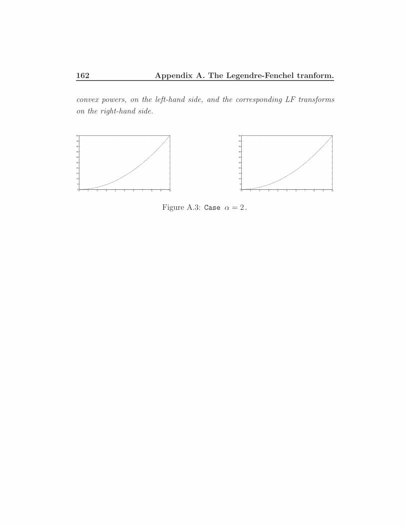
162 Appendix A. The Legendre-Fenchel tranform.
convex powers, on the left-hand side, and the corresponding LF transforms
on the right-hand side.
0 1 2 3 4 5 6 7 8 9 100
5
10
15
20
25
30
35
40
45
50
0 1 2 3 4 5 6 7 8 9 100
5
10
15
20
25
30
35
40
45
50
Figure A.3: Case α = 2.
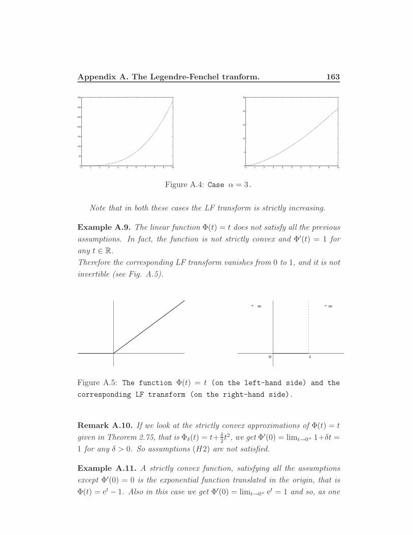
Appendix A. The Legendre-Fenchel tranform. 163
0 1 2 3 4 5 6 7 8 9 100
50
100
150
200
250
300
350
0 1 2 3 4 5 6 7 8 9 100
5
10
15
20
25
Figure A.4: Case α = 3.
Note that in both these cases the LF transform is strictly increasing.
Example A.9. The linear function Φ(t) = t does not satisfy all the previous
assumptions. In fact, the function is not strictly convex and Φ′(t) = 1 for
any t ∈ R.
Therefore the corresponding LF transform vanishes from 0 to 1, and it is not
invertible (see Fig. A.5).
10
+ 8 8+
Figure A.5: The function Φ(t) = t (on the left-hand side) and the
corresponding LF transform (on the right-hand side).
Remark A.10. If we look at the strictly convex approximations of Φ(t) = t
given in Theorem 2.75, that is Φδ(t) = t+ δ2t2, we get Φ′(0) = limt→0+ 1+δt =
1 for any δ > 0. So assumptions (H2) are not satisfied.
Example A.11. A strictly convex function, satisfying all the assumptions
except Φ′(0) = 0 is the exponential function translated in the origin, that is
Φ(t) = et − 1. Also in this case we get Φ′(0) = limt→0+ et = 1 and so, as one

164 Appendix A. The Legendre-Fenchel tranform.
0 1 2 3 4 5 6 7 8 9 100
0.5
1
1.5
2
2.5x 10
4
0 0.5 1 1.5 2 2.5 3 3.5 4 4.5 50
0.5
1
1.5
2
2.5
3
3.5
4
4.5
Figure A.6: The translated exponential function (on the left-hand
side) and its LF transform (on the right-hand side).
can see in Fig. A.6, the LF transform is not invertible in the interval [0, 1].
Remark A.12. For the functions given in Examples A.9 and A.11 the proof
of Theorem 2.75 does not hold.
Example A.13. We conclude giving an example of a non-standard function
satisfying (H2). So, let Φ(t) = et − t − 1, it is trivial that Φ(0) = 0 and
Φ′(0) = 1 − 1 = 0. Moreover Φ′(t) = et − 1 ≥ 0 and Φ′′(t) = et ≥ 1 > 0 for
any t ≥ 0, then Φ(t) is non decreasing and strictly convex.
0 0.5 1 1.5 2 2.5 3 3.5 4 4.5 50
50
100
150
0 0.5 1 1.5 2 2.5 3 3.5 4 4.5 50
1
2
3
4
5
6
Figure A.7: Φ(t) = et − t − 1 (on the left-hand side) and its LF
transform (on the right-hand side).
Bibliography
[1] J.F. Adams. Lectures on Lie Groups. Benjamin, New York, 1969.
[2] A. Agrachev, J.P. Gauthier. On the Dido problem and plane isoperimet-
ric problems. Acta Appl. Math. 57, N.3 (1999), 287-338.
[3] O. Alvarez, E.N. Barron, H. Ishii. Hopf-Lax formula for semicontinuous
data. Indiana University Math. J. 48, N.3 (1999), 993-1035.
[4] L. Ambrosio, S. Rigot. Optimal mass transportation in Heinsenberg
group. J. Funct. Anal. 208, N.2 (2004), 261-301.
[5] J.P. Aubin, A. Cellina. Differential Inclusions: Set-Valued Maps and
Viability Theory. Springer, Berlin, 1984.
[6] J.P. Aubin, H. Frankowska. Set-Valued Analysis. Birkhauser, Boston,
1990.
[7] M. Bardi, I. Capuzzo Dolcetta. Optimal Control and Viscosity Solutions
of Hamilton-Jacobi-Bellman Equations. Birkhauser, Boston, 1997.
[8] M. Bardi, L.C. Evans. On Hopf’s formulas for solutions of Hamilton-
Jacobi equations. Nonlinear Analysis Theory Methods and Applications
8, N.II (1984), 1373-1381.
[9] G. Barles. Existence results for first-order Hamilton-Jacobi equations.
Inst. H. Poincare Ann. Non Lineaire 1 (1984), 325-340.
[10] G. Barles. Discontinuous viscosity solutions of first-order Hamilton-
Jacobi equations: a guided visit. Nonlinear Anal. 20, N.9 (1993), 1123-
1134.
166 Bibliography.
[11] G. Barles. Solutions de Viscosite des Equations de Hamilton-Jacobi.
Springer-Verlag, Berlin, 1994.
[12] G. Barles, B. Perthame. Disontinuous solutions of deterministic optimal
stopping time problems. Math. Mod. Num. Analysis 21, N.4 (1987), 557-
579.
[13] G. Barles, B. Perthame. Exit time problems in optimal control and
vanishing viscosity method. SIAM J. Control Opt. 26, II (1988), 1133-
1148.
[14] E.N. Barron, R. Jensen. Semicontinuous viscosity solutions for
Hamilton-Jacobi equations with convex Hamiltonians. Comm. PDE 15,
N.12 (1990), 1173-1742.
[15] E.N. Barron, R. Jensen. Optimal control and semicontinuous viscosity
solutions. Proc. Am. Math. Soc. 133, N.2 (1991), 397-402.
[16] F. Baudoin. An introduction to the geometry of stochastic flows. Imperial
College press, London, 2004.
[17] A. Bellaıche. The tangent space in Sub-Riemmanian geometry, in Sub-
Riemannian Geometry, A. Bellaıche and J.J. Risler Editors, Basel,
Birkhauser, 1996.
[18] P. Bono, M.V. Tessitore. Il mito di Didone. Bruno Mondadori, Milano,
1998.
[19] S. Bortoletto. The Bellman equation for constrained deterministic opti-
mal control problems. Diff. Int. Eq. 6, N.4 (1993), 905-924.
[20] U. Boscain, G. Charlot, J.-P. Gauthier, S. Guerin, H.-R. Jauslin. Opti-
mal control in laser-induced population transfer for two- and three-level
quantum systems. J. Math. Physics 43, N.5 (2002).
[21] B.W. Brockett. Control Theory and Singular Riemannian Geometry,
New directions in applied mathematics. Springer, 1980.

Bibliography. 167
[22] H. Busemann. The Geometry of Geodesics. Academic Press, New York,
1955.
[23] X. Cabre, L.A. Caffarelli. Fully Nonlinear Elliptic Equations. AMS,
Colloquium Publications 45, Providence, 1995.
[24] P. Cannarsa, C. Sinestrari. Semiconcave Functions, Hamilton-Jacobi
Equations, and Optimal Control. Birkhauser, Boston, 2004.
[25] I. Capuzzo Dolcetta. The Hopf solution of Hamilton-Jacobi equations.
Elliptic and Parabolic Pb., 343-351, World Sci., River Edge, NJ, 2002.
[26] I. Capuzzo Dolcetta. Representations of solutions of Hamilton-Jacobi
equations. Progr. Nonlinear Diff. Eq. Appl. 54, Birkhauser, Basel, 2003.
[27] I. Capuzzo Dolcetta, H. Ishii. Hopf formulas for state dependent
Hamilton-Jacobi equations. preprint.
[28] C. Caratheodoty. Untersuchungen uber die grundlagen der thermody-
namik. Math. Ann. 67, N.3 (1909), 355-386.
[29] C. Chevalley. Theory of Lie Groups. Princeton University Press, Prince-
ton, 1946.
[30] W.L. Chow. Uber systeme von linearen partiellen differentialgleichungen
erster ordnung. Math. Ann. 117 (1939), 98-105.
[31] G. Citti, M. Manfredini. Blow-up in non-homogeneous Lie groups and
rectifiability. Huston J. Math. 31, N.2 (2005), 333-353.
[32] G. Citti, M. Manfredini. Uniform estimates of the fundamental solution
for a family of hypoelliptic operators,. Potential Analysis 25 (2006),
147-164.
[33] G. Citti, M. Manfredini, A. Sarti. From neural oscillations to variational
problems in the visual cortex. J. Physiology 97 (2003), 87-385.
[34] G. Citti, M. Manfredini, A. Sarti. Neuronal oscillation in the visual cor-
tex: Gamma-convergence to the Riemannian Mumford-Shah functional.
SIAM J. Math. Analysis 35, N.6 (2004), 1394-1419.
168 Bibliography.
[35] G. Citti, A. Sarti. A cortical based model of perceptual completion in the
roto-traslation space. Journal of Math. Imaging and Vision 24 (2006),
307-326.
[36] M.G. Crandall, L.C. Evans, P.L. Lions Some properties of viscosity so-
lutions of Hamilton-Jacobi equations. Trans. Am. Mat. Soc. 282 (1984),
487-502.
[37] M.G. Crandall, H. Ishii, P.L. Lions. Uniqueness of viscosity solutions of
Hamilton-Jacobi equations revisited. J. Math. Soc. Japan 39, N.4 (1987),
581-596.
[38] M.G. Crandall, H. Ishii, P.L. Lions. User’s guide to viscosity solutions
of second order partial differential equations. Bull. Am. Math. Soc. 27,
N.1 (1992), 1-67.
[39] M.G. Crandall, P.L. Lions. Condition d’unicite pour les solutions gener-
alisees des equations de Hamilton-Jacobi du premier ordre. C. R. Acad.
Sci. Paris Ser. I Math 292 (1981), 183-186.
[40] M.G. Crandall, P.L. Lions. Viscosity solutions of Hamiltonian-Jacobi
equations. Trans. Am. Math. Soc. 277 (1983), 1-42.
[41] M.G. Crandall, P.L. Lions. On existence and uniqueness of solutions
of Hamilton-Jacobi equations. Nonlinear Analysis Theory Appl. 10, N.4
(1986), 353-370.
[42] A. Cutrı, F. Da Lio. Comparison and uniqueness results for non-
coercitive first-order Hamilton-Jacobi equations. ESAIM-COCV 13, N.3
(2007), 484-502.
[43] A. Davini. Smooth approximation of weak Finsler metrics. Diff. Int. Eq.
18, N.5 (2005), 509-530.
[44] F. Dragoni. Metric Hopf-Lax formula with semicontinuous data. Discrete
and Continuous Dynamical Systems 17, N. 4 (2007), 713-729.
[45] F. Dragoni. Limiting behavior of solutions of subelliptic heat equations.
tNonlinear Diff. Equations and Applications 14, N.3-4 (2008), 429-443..
Bibliography. 169
[46] M.P. Do Carmo. Riemannian Geometry. Birkhauser, Basel, 1992.
[47] L.C. Evans. Partial Differential Equations. Am. Math. Soc., Providence
RI, 1988.
[48] S. Gallot, D. Hulin, J. Lafontaine. Riemannian Geometry. Springer-
Verlag, Berlin, 1990.
[49] B. Gaveau. Principe de moindre action, propagation de la chaleur et
estimees sous elliptiques sur certain groupes nilpotents. Acta Math. 139
(1977), 95-153.
[50] G. Gentili, F. Podesta, E. Vesentini. Lezioni di Geometria Differenziale.
Bollati Boringhieri, Torino, 1995.
[51] M. Gromov. Carnot-Caratheodory spaces seen from within, in Sub-
Riemannian Geometry, A. Bellaıche and J.J. Risler Editors, Basel,
Birkhauser, 1996.
[52] J. Heinonen. Calculus on Carnot Groups. Fall School in Analysis
(Jyvaskyla, 1994), 1-31.
[53] R. Hermann. Geodesics of singular Riemannian metrics. Bull. Am.
Math. Soc. 79 (1973), 780-782.
[54] E. Hopf. Generalized solutions of non-linear equations of first order. J.
Math. Mech. 14 (1965), 951-973.
[55] L. Hormander. Hypoelliptic second order differential operators. Acta
Math. 119 (1967), 147-171.
[56] H. Ishii. Hamilton-Jacobi equations. Bull. Fac. Sci. Eng. Chuo Univ. 28
(1985), 33-77.
[57] H. Ishii. Perron’s method for Hamilton-Jacobi equations. Duke Math. J.
55, N.2 (1987), 369-384.
[58] H. Ishii. Comparison results for Hamilton-Jacobi equations without
growth condition on solutions from above.Appl. Anal. 67 (1997), 357-372.

170 Bibliography.
[59] H. Ishii. A generalization of a theorem of Barron and Jensen and a
comparison theorem for lower semicontinuous viscosity solutions. Proc.
Roy. Soc. Edimburg Sect. A 131, N.1 (2001), 137-151.
[60] D.S. Jerison, A. Sanchez-Calle. Estimates for the heat kernel for a sum
of squares of vector fields. Indiana Univ. Math. J. 35, N.4 (1986), 835-
854.
[61] A.E. Kogoj, E. Lanconelli. X-elliptic operators and X-controll distances.
Ricerche di Matematica Supplemento 49 (2000), 223-243.
[62] A.E. Kogoj, E. Lanconelli. One-side Liouville theorems for a class of
hypoelliptic ultraparabolic equations. Geom. An. PDE several complex
variables 368 (2005), 305-312.
[63] S. Kusuoka, D. Stroock. Applications of Malliavin calculus, part III. J.
Fac. Sci. Univ. Tokyo Sect. 1A Math. 34, N.2 (1987), 391-442.
[64] S. Kusuoka, D. Stroock. Long time estimates for the heat kernel associ-
ated with a uniformly suelliptic symmetric second order operator. Ann.
Math. 127, N.1 (1998), 165-189.
[65] E. Lanconelli, A. Pascucci. On the fundamental solution for hypoelliptic
second order partial differential equations with non-negative character-
istic form. Ricerche Mat. 48, N.1 (1999), 81-106.
[66] J.M. Lasry, P.L. Lions. A remark on regularization in Hilbert spaces.
Israel J. of Math. 55, N.3 (1986), 257-266.
[67] R. Leandre. Majoration en temps petit de la densite d’une diffusion
degeneree. Prob. Theory Related Fields 74, N.2 (1987), 289-294.
[68] R. Leandre. Minoration en temps petit de la densite d’une diffusion
degeneree. Journal of Functional Analysis 74, N.2 (1987), 399-414.
[69] P. Li, S.T. Yau. On the parabolic kernel of the Schrodinger operator.
Acta Math. 156, N.3-4 (1986), 153-201.
[70] E.H. Lieb, M. Loss. Analysis. Am. Math. Soc., Providence, 1997.

Bibliography. 171
[71] P.L. Lions. Generalized Solutions of Hamilton-Jacobi Equations. Re-
search Notes in Mathematics 69, Pitman, 1982.
[72] W. Liu, H.J. Sussmann. Shortest paths for sub-Riemannian metrics on
rank-two distributions. Mem. Am. Math. Soc. 118 (1995), 0-104.
[73] G. Lu, J.J. Manfredi, B. Stroffolini. Convex functions on the Heisenberg
group. Calc. Var. 19 (2004), 1-22.
[74] J.J. Manfredi, B. Stroffolini. A version of the Hopf-Lax formula in the
Heisenberg group. Comm. in Part. Diff. Eq. 27, N.5-6 (2002), 1139-1159.
[75] R. Montgomery. A Tour of Subriemannian Geometries, Their Geodesics
and Application. Am. Math. Soc., United States of America, 2002.
[76] R. Monti. Distances, boundaries and surface measures in Carnot-
Caratheodory spaces. PDh Thesis, University of Trento, 1994.
www.unitn.it/dipartiment/mate/download/tesi dott.doc.
[77] R. Monti, F. Serra Cassano. Surface measures in Carnot-Caratheodory
spaces. Calc. Var. Part. Diff. Eq. 13, N.3 (2001), 339-376.
[78] A. Nagel, E.M. Stein, S. Wainger. Balls and metrics defined by vector
fields I: basic properties. Acta Math. 155 (1985), 103-147.
[79] K. Nomizu. Lie Gruops and Differential Geometry. Math. Soc. of Japan,
Tokyo, 1956.
[80] P. Pansu. Metriques de Carnot-Caratheodory et quasi isometries des
espaces symmetriques de rang un. Ann. Math. 129 (1989), 1-60.
[81] O. Perron. Eine neue Behandlung der Randwertufgabe fur ∆u = 0.
Math. Z. 18 (1923), 42-54.
[82] P.K. Rashevsky. Any two points of a totally nonholonomic space may be
connected by an admissible line. Uch. Zap. Ped. Inst. Im. Liebknechta
(Russian), Ser. Phys. Math. 2 (1938), 83-94.
[83] R.T. Rockafellar. Convex Analysis. Princeton University Press, Prince-
ton, 1997.
172 Bibliography.
[84] A. Sanchez-Calle. Fundamental solutions and geometry of the sum of
squares of vector fields. Invent. Math. 78 (1984), 143-160.
[85] S. Semmes. On the nonexistence of bi-Lipschitz parametrizations and
geometric about A∞-weights. Revista Matematıca Iberoamericana 12,
N.2 (1996) 337-410.
[86] A. Siconolfi. Metric character of Hamilton-Jacobi equations. Trans. Am.
Math. Soc. 355, N.5 (2003), 1987-2009.
[87] P.E. Souganidis. Existence of viscosity solutions of Hamilton-Jacobi
equations. J. Diff. Eq. 56 (1985), 345-390.
[88] E.M. Stein. Singular integrals and differentiability properties of func-
tions. Princeton University Press, Princeton, 1970.
[89] R.S. Strichartz. Sub-Riemannian geometry. Diff. Geom. 24 (1986), 221-
263.
[90] H. Touchette. Legendre-Fenchel transform in a nutshell.
www.maths.qmul.ac.uk/ ht/archive1/lfth2.pdf.
[91] V.S. Varadarajan. Lie Groups, Lie Algebras, and Their Rappresenta-
tions. Springer-Verlag, New York, 1984.
[92] S.R.S. Varadhan. On the behavior of the fundamental solution of the
heat equation with variable coefficients. Comm. Pure Appl. Math. 20
(1967), 431-455.
[93] S.R.S. Varadhan. Diffusion Processes in a Small Time Interval. Comm.
Pure Appl. Math. 20 (1967), 659-685.
[94] S.R.S. Varadhan. Large Deviations and Applications. Soc. for Industrial
and Applied Math., Philadelphia PA, 1984.
[95] A.M. Vershik, V. Ya Gershkovich. Nonholonomic dynamical systems,
geometry of distributions and variational problems, in Dynamical System
VII. V.I. Arnold, S.P. Novikov, Encyclopedia of Math. Sciences 16,
Springer, 1994.


![[Papercraft] Orca](https://img.dokumen.tips/doc/110x75/552887e04a7959d8448b4789/papercraft-orca.jpg)