Phantom black holes in Einstein-Maxwell-dilaton theory

Phantom black holes in Einstein-Maxwell-dilaton theory

Gerard Clement,1,* Julio C. Fabris,2,3,† and Manuel E. Rodrigues1,2,‡

1LAPTH, Laboratoire d’Annecy-le-Vieux de Physique Theorique,9, Chemin de Bellevue—BP 110, 74941 Annecy-le-Vieux CEDEX, France

2Universidade Federal do Espırito Santo, Centro de Ciencias Exatas—Departamento de Fısica,Av. Fernando Ferrari s/n—Campus de Goiabeiras, CEP29075-910—Vitoria/ES, Brazil

3IAP, Institut d’Astrophysique de Paris, 98bis, Bd Arago—75014 Paris, France(Received 3 February 2009; published 20 March 2009)

We obtain the general static, spherically symmetric solution for the Einstein-Maxwell-dilaton system in

four dimensions with a phantom coupling for the dilaton and/or the Maxwell field. This leads to new

classes of black hole solutions, with single or multiple horizons. Using the geodesic equations, we analyze

the corresponding Penrose diagrams revealing, in some cases, new causal structures.

DOI: 10.1103/PhysRevD.79.064021 PACS numbers: 04.70.Bw, 04.40.Nr, 11.25.Mj

I. INTRODUCTION

Effective gravity actions emerging from string andKaluza-Klein theories contain a rich structure where, be-side the usual Einstein-Hilbert term, there is a scalar field,generically called a dilaton, coupled to an electromagneticfield. The asymptotically flat static black hole solutions forthis Einstein-Maxwell-dilaton (EMD) system [1,2] differfrom the usual Reissner-Nordstrom solution of Einstein-Maxwell theory in that the inner horizon is singular for anonvanishing dilaton coupling. Nonasymptotic flat staticblack hole solutions have also been obtained in [3] andfurther studied in [4–6]. Brane configurations, leading alsoto black hole solutions, have been largely studied inRef. [7,8] using essentially the EMD theory.

The aim of the present work is to study the structures ofthe black holes of the EMD theory when a phantomcoupling is considered. This is done by allowing the scalarfield or the Maxwell field (or both) to have the ‘‘wrong’’sign [9]. The importance of such extension of the normal(nonphantom) EMD theory is twofold. First, from thetheoretical point of view, string theories admit ghost con-densation, leading to phantom-type fields [10]. In princi-ple, a phantom may lead to instability, mainly at thequantum level. But there are claims that these instabilitiescan be avoided [11]. The second motivation comes fromthe results of the observational programs of the evolutionof the Universe, specially the magnitude-versus-redshiftrelation for the supernovae type Ia, and the anisotropyspectrum of the cosmic microwave background radiation:both observational programs suggest that the universe to-day must be dominated by an exotic fluid with negativepressure. Moreover, there is some evidence that this fluidcan be phantom [12,13].

When the scalar field and/or the Maxwell field areallowed to contribute negatively to the total energy, the

energy conditions (and specially the null energy condition�þ p � 0) can be violated, and the appearance of somenew structures can be expected. This is the case of worm-hole solutions to Einstein-scalar [14] or Einstein-Maxwell-scalar [15] theory with a phantom scalar field. Anotherinstance is that of black hole solutions to Einstein theoryminimally coupled to a free scalar field, which are forbid-den by the no-hair theorem, but become possible if thekinetic term of the scalar field has the wrong sign (if thescalar field is phantom), as found both in 2þ 1 [16] and in3þ 1 dimensions [17]. These phantom black holes have allthe characteristics of the so-called cold black holes [18,19]:a degenerate horizon (implying a zero Hawking tempera-ture) and an infinite horizon surface. Indeed, these coldblack holes appeared in the context of scalar-tensor theory(e.g., in Brans-Dicke theory) in such circumstances that,after reexpressing the action in the Einstein frame, thescalar field comes out to be phantom.The nontrivial dilatonic coupling of the scalar field with

the electromagnetic term adds new classes of black holesolutions. In Refs. [9,20] some investigations on phantomblack holes in the context of EMD theory have been made,revealing some interesting new species of black holes. Forexample, in the case of a self-interacting scalar field in fourdimensions, a phantom field may lead to a completelyregular spacetime where the horizon hides an expanding,singularity-free universe [21]. Our goal here is to obtain themost general static black hole solutions when a phantomcoupling is allowed for both the scalar and electromagneticfields of the EMD theory.We will classify the different possible black hole solu-

tions coming out from the EMD theory for a phantomcoupling of either the dilaton field, of the Maxwell field,or of both. It is remarkable that many of these new blackholes have a degenerate horizon, hence a zero Hawkingtemperature. We will also analyze the causal structure ofthese black hole spacetimes. In some cases, the causalstructure is highly unusual, such that no two-dimensionalPenrose diagram can be constructed. Another possibility is

*[email protected]†[email protected]‡[email protected]

PHYSICAL REVIEW D 79, 064021 (2009)

1550-7998=2009=79(6)=064021(13) 064021-1 � 2009 The American Physical Society

http://dx.doi.org/10.1103/PhysRevD.79.064021

that of a spacetime with an infinite series of regular hori-zons separating successive nonisometric regions.Geodesically complete black hole spacetimes are alsoobtained.

This paper is organized as follows. In the next section wederive, following the procedure of [22], the general staticspherically symmetric solutions (phantom and nonphan-tom) of the EMD theory. In Sec. III the new black holesolutions are described in detail. The Penrose diagrams ofthese new solutions are constructed in Sec. IV. In Sec. V wepresent our conclusions.

II. GENERAL SOLUTION

Let us consider the following action:

S ¼Z

dx4ffiffiffiffiffiffiffi�g

p ½R� 2�1g��r�’r�’

þ �2e2�’F��F��; (2.1)

which is the sum of the usual Einstein-Hilbert gravitationalterm, a dilaton field kinetic term, and a term coupling theMaxwell Lagrangian density to the dilaton, with the cou-pling constant � real. The dilaton-gravity coupling con-stant �1 can take either the value �1 ¼ 1 (dilaton) or�1 ¼ �1 (antidilaton). The Maxwell-gravity couplingconstant �2 can take either the value �2 ¼ 1 (Maxwell)or �2 ¼ �1 (anti-Maxwell). This action leads to the fol-lowing field equations:

r�½e2�’F�� ¼ 0; (2.2)

h’ ¼ � 1

2�1�2�e

2�’F2; (2.3)

R�� ¼ 2�1r�’r�’þ 2�2e2�’

�1

4g��F

2 � F��F��

�:

(2.4)

Let us write the static, spherically symmetric metric as

dS2 ¼ e2�ðuÞdt2 � e2�ðuÞdu2 � e2ðuÞd�2: (2.5)

The metric function � can be changed at will by redefin-ing the radial coordinate. In the following we will assumethe harmonic coordinate condition

� ¼ 2þ �: (2.6)

We will also assume the Maxwell field to be purelyelectric (the purely magnetic case may be obtained fromthis by the electric-magnetic duality transformation ’ !�’, F ! e�2�’ � F). Integrating (2.2), we obtain

F10ðuÞ ¼ qe�2ð�’þ2þ�Þ ðF2 ¼ �2q2e�4�4�’Þ;(2.7)

with q a real integration constant. Replacing (2.7) intoequations, we obtain the second order equations

’00 ¼ ��1�2�q2e2!; (2.8)

�00 ¼ �2q2e2!; (2.9)

00 ¼ e2J � �2q2e2!; (2.10)

with

! ¼ �� ’; J ¼ �þ ; (2.11)

and the constraint equation

02 þ 20�0 � �1’02 ¼ e2J � �2q

2e2!: (2.12)

By taking linear combinations of the Eqs. (2.8), (2.9),and (2.10), this system can be partially integrated to

’ðuÞ ¼ ��1��ðuÞ þ ’1uþ ’0; (2.13)

!02 �Qe2! ¼ a2; (2.14)

J02 � e2J ¼ b2; (2.15)

where

�� ¼ ð1� �1�2Þ; Q ¼ �2�þq2; (2.16)

and the integration constants ’0, ’1 2 R, a, b 2 C.The general solution of (2.14) is:

!ðuÞ¼

8>>>>>><>>>>>>:

�lnj ffiffiffiffiffiffiffijQjpa�1cosh½aðu�u0Þ�j ða2Rþ;Q2R�Þ;

aðu�u0Þ ða2Rþ;Q¼0Þ;�lnj ffiffiffiffi

Qp

a�1sinh½aðu�u0Þ�j ða2Rþ;Q2RþÞ;�lnj ffiffiffiffi

Qp ðu�u0Þj ða¼0;Q2RþÞ;

�lnj ffiffiffiffiQ

p�a�1sin½ �aðu�u0Þ�j ða¼i �a; �a;Q2RþÞ

(2.17)

(u0 real constant). The general solution of (2.15) is:

JðuÞ ¼8<:� lnjb�1 sinh½bðu� u1Þ�j ðb 2 RþÞ;� lnju� u1j ðb ¼ 0Þ;� lnj �b�1 sin½ �bðu� u1Þ�j ðb ¼ i �b; �b 2 RþÞ

(2.18)

(u1 real constant).In this way, we have for �þ � 0 the general solution of

the theory given by the action (2.1):

dS2 ¼ e2�dt2 � e2�du2 � e2d�2;

�ðuÞ ¼ 2JðuÞ � �ðuÞ;ðuÞ ¼ JðuÞ � �ðuÞ;�ðuÞ ¼ ��1þ ð!ðuÞ þ �’1uþ �’0Þ;’ðuÞ ¼ ��1þ ð��1�!ðuÞ þ ’1uþ ’0Þ;

F ¼ �qe2!ðuÞdu ^ dt; (2.19)

where the integration constants should be related by theconstraint (2.12). We will analyze the case �þ ¼ 0 (�1 ¼

CLEMENT, FABRIS, AND RODRIGUES PHYSICAL REVIEW D 79, 064021 (2009)

064021-2

�1, �2 ¼ 1), for which the function !ðuÞ is linear, inSec. III B.

In the limit u ! u1, the function JðuÞ goes to þ1,corresponding from (2.18) to spacelike infinity. So thereare a priori two disjoint solution sectors u� u1 > 0 andu� u1 < 0. However the ansatz (2.5) is form-invariantunder the symmetry u� u1 ! �ðu� u1Þ, which allowsus to select e.g. the solution sector

u < u1: (2.20)

Invariance of the metric ansatz under translations of theradial coordinate u also enables us to fix e.g. the integrationconstant

u1 ¼ 0: (2.21)

The solution (2.19) then depends on the 6 parametersðq; a; b; u0; ’0; ’1Þ which are related by the constraintequation following from (2.12),

�þb2 ¼ a2 þ �1’21: (2.22)

Moreover, two of the parameters may be fixed by im-posing that at infinity the space-time is Minkowskian andthe dilaton field vanishes. Hence, we end up with threeindependent parameters. Later, imposing the analyticity ofthe solution across the horizon, the number of free parame-ters will be reduced to only two.

All solutions written above with �1 and �2 positive (thenonphantom case) have already been determined previ-ously (see for example [22] and references therein). Toour knowledge, only the phantom solutions with nonde-generate horizon have already been determined.

III. NEW BLACK HOLE SOLUTIONS

From (2.17) and (2.18), with u < 0 according to (2.20),we have 15 different solutions which combine to form thesolution (2.19). The first and second solutions (2.17) arenecessarily phantom (�1 ¼ �1 and/or �2 ¼ �1). Theother ones can be normal (�1 ¼ �2 ¼ 1), or phantom,(�1 ¼ �2 ¼ �1, �2 > 1 or �1 ¼ ��2 ¼ �1, �2 < 1).As for the function JðuÞ, only the first solution (2.18)occurs in the normal case. This is because if b ¼ i �b ( �breal)1 the constraint (2.22) can be written

a2 þ �b2 ¼ ��1ð’21 þ �2 �b2Þ; (3.1)

implying �1 ¼ �1 (antidilaton case). In this section wewill discuss the new black hole solutions, classified accord-ing to the type of the solution (2.17) for !ðuÞ.

A. The cosh solution

The metric function e2� for the choice of the first solu-tion (2.17) can vanish only for u ! �1, corresponding tothe event horizon. The third solution (2.18) for J obviously

leads to a metric which is defined only in finite intervals (inbetween zeroes of the sine), so it cannot have a horizon. Asfor the second solution (2.18), it can be written

dS2 ¼ e2�dt2 � e�2�ðdr2 þ r2d�2Þ ðr ¼ �1=uÞ;(3.2)

showing that the horizon u ! �1 (r ¼ 0) is actuallysingular. So we restrict ourselves to the first solution(2.18).To study the near-horizon behavior of the metric, it is

useful to transform to a radial coordinate proportional tothe near-horizon geodesic affine parameter. From theLagrangian for geodesic motion

L ¼ 1

2g�� _x

� _x�; (3.3)

we obtain the first integral for geodesic motion in theequatorial plane

e4J _u2 ¼ E2 � e2�½þ L2e�2�; (3.4)

where E is the momentum conjugate to time (energy), L isthe momentum conjugate to the azimutal angle (angularmomentum), and ¼ 1 for timelike geodesics, ¼ 0 fornull geodesics and ¼ �1 for spacelike geodesics. On theevent horizon this equation becomes

ds� e2Jdu� b2e2budu: (3.5)

This suggests performing the coordinate transformation

x ¼ e2bðu�u0Þ; (3.6)

leading to the line element

dS2 ¼ cxn

ð1þ xmÞ2=�þdt2 � 4b2x1x

1�nð1þ xmÞ2=�þ

cðx� x1Þ2

��

x1dx2

xðx� x1Þ2þ d�2

�; (3.7)

where according to (2.20) x < x1, with x1 ¼ e�2bu0 , c > 0is a constant which can be fixed so that the metric isasymptotically Minkowskian, and

m ¼ a

b; n ¼ mð1þ � �’1Þ

�þ(3.8)

( �’1 ¼ ’1=a). This spacetime is asymptotically flat, withthe spatial infinity at x ¼ x1 (u ¼ 0) and the event horizonat x ¼ 0. It is clear that the metric is analytic near the eventhorizon only if m and n are positive integers [16,18].The definition of n and the constraint Eq. (2.22) may be

rewritten as

1þ � �’1 ¼ �þn

m; 1þ �1 �’

21 ¼

�þm2

: (3.9)

The first equation relates the integration constant �’1 tothe black hole quantum numbers n and m. Eliminating thisconstant between the two relations (3.9), we obtain the1This includes the case b ¼ 0.

PHANTOM BLACK HOLES IN EINSTEIN-MAXWELL- . . . PHYSICAL REVIEW D 79, 064021 (2009)

064021-3

relation

m ¼ n� �ffiffiffiffiffiffiffiffiffiffiffiffiffiffiffiffiffiffiffiffiffiffiffi�1ð1� n2Þ

q: (3.10)

The implications of this relation depend on the value ofthe horizon degeneracy degree n. If n ¼ 1 (nondegeneratehorizon), then necessarily also m ¼ 1; this can occur forany real � (with�1 and�2 such that�2�þ < 0). But if n �2 (degenerate horizon), which is only possible in the anti-dilaton case�1 ¼ �1, then relation (3.10) gives the dilatoncoupling constant � in terms of the black hole ‘‘quantumnumbers’’ m and n:

�2 ¼ ðm� nÞ2n2 � 1

: (3.11)

This is such that �2 < 1 (�2 ¼ �1) if 1 � m � 2n� 1,and �2 > 1 (�2 ¼ þ1) if m � 2n.

Conversely, for a given value of the model parameters in(2.1), there are three possibilities. Either �1¼þ1 or�1¼�1 but � does not belong to the discrete set of values(3.11), and the only black hole solution is nondegenerate(m ¼ n ¼ 1); or �1 ¼ �1 and � � 0 belongs to this dis-crete set (with the appropriate sign for �2), and we havetwo distinct black hole solutions, one degenerate, the othernondegenerate. Finally there is the third possibility � ¼ 0with �1 ¼ �2 ¼ �1, leading to a tower of degenerateblack hole solutions with m ¼ n above the ground non-degenerate black holem ¼ n ¼ 1. Let us note that this lastcase corresponds to the (nondilatonic) Einstein-anti-Maxwell theory with an additional massless scalar fieldcoupled repulsively to gravity. Recall that in the normalcase (�1 ¼ þ1), the second Eq. (3.9) with �þ ¼ 1 has theonly solution m ¼ 1 with �’1 ¼ 0, leading to the Reissner-Nordstrom black hole with constant scalar field. This is thewell-known no-hair theorem, which is no longer true in thepresent phantom (antiscalar) case.

To put the cosh solution in a more familiar form, we usethe coordinate transformation [22],

u ¼ 1

ðrþ � r�Þ ln�fþf�

�; f� ¼ 1� r�

r; (3.12)

with

r� ¼ � 2a

1þ e2au0ðrþ � r� ¼ 2aÞ: (3.13)

The coordinate x defined by (3.6) is related to r by

xm ¼ � r�fþrþf�

: (3.14)

In the case of a nondegenerate horizon (n ¼ m ¼ 1), thesolution takes the following form:

dS2 ¼ fþf��=�þ� dt2 � f�1þ f�ð��=�þÞ� dr2

� r2f1�ð��=�þÞ� d�2;

F ¼ � q

r2dr ^ dt; e�2�’ ¼ f1�ð��=�þÞ� ; (3.15)

where we have chosen the integration constants so that atspatial infinity the metric is Minkowskian and the dilatonvanishes, i.e. ’0 ¼ !ð0Þ ¼ 0 in (2.19). The correspondingblack hole mass M and charge q are

M ¼ 1

2

�rþ þ ��

�þr�

�; q ¼ �

ffiffiffiffiffiffiffiffiffiffiffiffirþr��2�þ

s: (3.16)

The solution (3.15) has the same form as the normalblack hole solution of [1,2], the only difference being thathere we have rþ > 0 but r� < 0. It was previously ob-tained by analytic continuation of the normal solution byGibbons and Rasheed [9] in the cases (�2 ¼ �1, �1 ¼þ1), and �1 ¼ �1 with �2 ¼ þ1 (for a2 > 1) or �2 ¼�1 (for a2 < 1), and was later generalized to higher-dimensional black holes (in the antidilaton case �1 ¼ �1with �2 ¼ þ1) by Gao and Zhang [20], and to higher-dimensional black branes by Grojean et al. [7].For the case of a degenerate horizon (�1 ¼ �1), per-

forming the transformation (3.12), we obtain the form(valid only outside the horizon, r > rþ)

dS2 ¼ gnþg��n� dt2 � ðrþ � r�Þ2m2

g1�nþ g1þn��ðgþ � g�Þ2

��ðrþ � r�Þ2ðgþg�Þ1�2m

m2r4ðgþ � g�Þ2dr2 þ d�2

�; (3.17)

F ¼ � q

r2dr ^ dt; e�2�’ ¼ gm�nþ gmþn�� ; (3.18)

where g� ¼ f1=m� , and

� ¼ 2m

�þ¼ 2mð1� n2Þ

ðm� nÞ2 þ 1� n2; (3.19)

with the mass and charge

M ¼ 1

2m½nrþ þ ð�� nÞr��; q ¼ �

ffiffiffiffiffiffiffiffiffiffiffiffirþr��2�þ

s: (3.20)

B. The linear solution

In the special case � ¼ �1 and �1 ¼ �1, the constant�þ vanishes, and !ðuÞ is given by the second solution(2.17), which depends linearly on the u coordinate. Inthis case, the functions �ðuÞ and’ðuÞ in (2.19) are replacedby

�ðuÞ ¼ �1uþ �0 þ q12e2aðu�u0Þ; (3.21)


064021-4

’ðuÞ ¼ ��ð�1 � aÞuþ ð�0 þ au0Þ þ q1

2e2aðu�u0Þ

�;

(3.22)

where �0 and �1 are integration constants, and q1 ¼�2q

2=2a2. Choosing again the sinh solution in (2.18),and performing the coordinate transformation (3.6), weobtain the metric,

dS2 ¼ cxn exp½q1xm�dt2 � 4b2x1x1�n

cðx� x1Þ2exp½�q1x

m�

��

x1dx2


�;

(3.23)

where again x1 ¼ e�2bu0 , c > 0, and

m ¼ a

b; n ¼ �1

b: (3.24)

As in the case of the cosh solution, the space-time isasymptotically flat, with the spatial infinity at x ¼ x1 andthe event horizon at x ¼ 0. Again, for the metric to beanalytic near the event horizon, the constantsm and nmustbe positive integers. These are not independent, because ofthe constraint (2.22) which now reads

b2 � að2�1 � aÞ ¼ 0 ) mð2n�mÞ ¼ 1: (3.25)

This is just the relation (3.11) for �2 ¼ 1, and it is clearthat its only solution in terms of integers is m ¼ n ¼ 1.Performing the transformations x ¼ x1fþ, with fþ ¼ 1�rþ=r, rþ ¼ 2b, we recover the linear solution previouslydiscussed by Gibbons and Rasheed [9] and by Gao andZhang [20]:

dS2 ¼ fþ exp½q1ðfþ � 1Þ�dt2 � exp½�q1ðfþ � 1Þ�

��dr2

fþþ r2d�2

�; (3.26)

F ¼ � q

r2dr ^ dt; e�2�’ ¼ exp½�q1ðfþ � 1Þ�;

(3.27)

with

M ¼ 1þ q12

rþ; q ¼ �rþffiffiffiffiffiffiffiffiffiffiffi�2q12

r: (3.28)

C. The phantom sinh solutions

The third solution (2.17) leads to a larger spectrum ofphantom black holes, with �1 < 0 (�1 > 0 with Q> 0implies �2 > 0, leading to normal black holes). The eventhorizon can correspond either to u ! �1, with only thefirst solution (2.18) for JðuÞ, or (if �þ < 0) to u ¼ u0, withthe three possibilities (2.18). There is also in the first casethe possibility of a nonasymptotical flat black hole space-

time when the singularity u ¼ u0 of the metric coincideswith spacelike infinity u ¼ 0 [8].We first consider the case where JðuÞ is given by the first

expression of (2.18). Performing as in the cosh case thecoordinate transformation (3.6), we obtain the followingline element:

dS2 ¼ cxn

j1� xmj2=�þdt2 � 4b2x1x

1�nj1� xmj2=�þ

cðx� x1Þ2

��

x1dx2


�;

(3.29)

where again x < x1 with x1 ¼ e�2bu0 , and c > 0. Thereal numbers m and n, given by (3.8), are again related by(3.10). There are three possibilities according to the rela-tive values of x1 and 1.(a) If x1 < 1 (u0 > 0), the event horizon is located at

x ¼ 0. As in the cosh case, this is regular if both mand n are integer. The discussion on the possibilityof degenerate horizons is identical to that followingEq. (3.10), provided that �2 is replaced by ��2

(�2�þ is positive in the sinh case). Performing thecoordinate transformation (3.12), with

r� ¼ � 2a

1� e2au0ðrþ � r� ¼ 2aÞ; (3.30)

we recover in the case m ¼ n ¼ 1 the metric (3.15),with now 0< r� < rþ. These solutions were pre-viously obtained in [9]. For the cases with degener-ate horizon (�1 ¼ �1, n � 2), we obtain thefunctional form (3.17).

(b) In the intermediate case x1 ¼ 1 (u0 ¼ 0), the eventhorizon is located, as in the first case, at x ¼ 0, withm and n integer. However the resulting solution is nolonger asymptotically flat [8]. Performing the coor-

dinate transformation x ¼ fþ with rþ ¼ 2bc�1=2

and rescaling the time coordinate, (3.29) becomes:

dS2 ¼ fnþð1� fmþÞ2=�þ

dt2 � ð1� fmþÞ2=�þ

fnþ� ½dr2 þ rðr� rþÞd�2�: (3.31)

This has the asymptotic behavior

dS2 ��r

rþ

�2=�þ

dt2 ��r

rþ

��2=�þðdr2 þ r2d�2Þ;ðr ! 1Þ (3.32)

with 0< �þ � 1 for �2>0, and �þ<0 for �2 < 0.(c) If x1 > 1 (u0<0), then the spacetime is asymptoti-

cally flat, but the event horizon is located at x¼1,provided �þ<0, implying both �1<0 and �2<0,together with �2>1. This is regular if �þ ¼ �2=p,i.e.


064021-5

�2 ¼ pþ 2

p; (3.33)

with p positive integer (but m and n no longernecessarily integer).This possibility also occurs when the second or thirdsolution (2.18) are combined with the third solution(2.17) with u0 < 0. In these cases the coordinatetransformation (3.6) leads to an unwieldy form ofthe metric. A more manageable expression for themetric in these three cases with u0 < 0 is

dS2 ¼ chpdt2 � c�1h�pe2Jðe2Jdu2 þ d�2Þ;(3.34)

with

hðuÞ ¼ e��’1u sinhaðu� u0Þ; (3.35)

e2JðuÞ ¼ b2

sinh2bu; or

1

u2; or

�b2

sin2 �bu:

(3.36)

D. The a ¼ 0 solutions

If u0 � 0, the event horizon is again at u ! �1 pro-vided JðuÞ is given by the first or second solution (2.18). Inthe first case (b2 > 0), the coordinate transformation (3.6)puts the metric in a form similar to (3.29), with n ¼ð�=�þÞð’1=bÞ and m ! 0, so that xm is replaced by alogarithm, which is clearly nonanalytic. So this possibilitydoes not lead to a regular black hole. In the case a ¼ b ¼ 0(implying ’1 ¼ 0), the coordinate transformation u ¼�1=r leads to the metric

dS2 ¼�

u0r

1þ u0r

�2=�þ

dt2

��

u0r

1þ u0r

��2=�þðdr2 þ r2d�2Þ; (3.37)

which is analytic if �þ ¼ 2=ðpþ 1Þ (p positive integer),implying �2 > 0, so that the phantom case corresponds to�1 < 0, and

�2 ¼ p� 1

pþ 1: (3.38)

Note that this is a special case of relation (3.11) for m ¼1, n ¼ p.

If on the other hand u0 < 0, the event horizon is at u ¼u0 and is regular if �þ ¼ �2=p with p a positive integer.Again, this implies �1 < 0, �2 < 0, and �2 > 1. The con-straint (2.22) reduces in this case to b2 ¼ p’2

1=2 � 0. Theresulting metric is of the form (3.34) with

hðuÞ ¼ e��’1uðu� u0Þ: (3.39)

For b ¼ 0 (’1 ¼ 0), the coordinate transformation u ¼�1=r leads to the particularly simple form of the metric

dS2 ¼ fpþdt2 � f�pþ ðdr2 þ r2d�2Þ; (3.40)

with rþ �1=u0.

E. The sin solution

In this case the metric is only defined in finite intervalsand so cannot have a horizon at u ! �1. Again, the eventhorizon can only be at u ¼ u0 < 0, and is regular if �þ ¼�2=p (p positive integer). The constraint (2.22) becomesin this case

2b2

p¼ �a2 þ ’2

1; (3.41)

so that necessarily b2 > 0, corresponding to the first solu-tion (2.18) for JðuÞ. The resulting metric can be put in theform (3.34), with

hðuÞ ¼ e��’1uj sin �aðu� u0Þj; (3.42)

e2JðuÞ ¼ b2

sinh2bu: (3.43)

IV. GEODESICS AND THE PENROSE DIAGRAMS

A. The cosh solution

The global structure of the new black hole spacetimesmay be determined by analyzing the geodesic Eq. (3.4),written in terms of the x coordinate of (3.7),

4b2x21 _x2

ðx� x1Þ4¼ E2 � cxn

ð1þ xmÞ2=�þ

��þ L2cxn�1ðx� x1Þ2

4b2x1ð1þ xmÞ2=�þ

�; (4.1)

together with the conformal form of the metric (3.7),

dS2 ¼ HðxÞ½dt2 � dy2 � FðxÞd�2�; (4.2)

with

dy ¼ � 2bx1c

x�nð1þ xmÞ2=�þ

ðx� x1Þ2dx; (4.3)

HðxÞ ¼ cxn

ð1þ xmÞ2=�þ; (4.4)

FðxÞ ¼ 4b2x1c2

x1�2nð1þ xmÞ4=�þ

ðx� x1Þ2: (4.5)

The various limits which should be analyzed are x ! x1(the spatial infinity), x ! 0 (the event horizon), as well aspossible coordinate singularities at x ! �1 and x ! �1.In the limit x ! x1, we obtain y ! �1, with FðxÞ ¼ y2

and H ¼ cst, showing that the metric (4.2) is asymptoti-


064021-6

cally Minkowskian. In the limit x ! 0, on the other hand,we obtain y ! �1 and H ! 0. This characterizes a hori-zon, in the present case the event horizon of the black holewhich, as previously discussed, is regular for all integervalues of n and m.

The analysis of the other possible coordinate singular-ities, at x ! �1 or x ! �1 depends on the parity of m.Let us summarize the different cases.

(1) m even. In this case, the metric (4.2) is regular atx ¼ �1, which corresponds to a finite value of y.The nature of the coordinate singularity at x ! �1depends on the value of �þ.

(a) If �þ < 0, (�2 > 1, which implies from (3.10) n <ðm2 þ 1Þ=2m, i.e. n � m=2) then H ! 1 and y !0. Hence, this is a center, a singularity where thegeodesics stop. If n is odd the Penrose diagram issimilar to the Schwarzschild diagram (Fig. 1), sincethere is an inversion of the light cone due to thechange of signature ðþ ��Þ ! ð�þ��Þ. If nis even, the two-dimensional light cone remainsunchanged, so that the Penrose diagram is similarto the extreme Reissner-Nordstrom diagram (Fig. 2).However the full four-dimensional signature doeschange when the horizon is crossed, ðþ ��Þ !ðþ�þþÞ, so that geodesic motion in this space-time should differ significantly from that in extremeReissner-Nordstrom spacetime (see the discussionin [18]).

(b) If �þ > 0 (n > m=2), we note that Eq. (3.10) im-plies

�þ ¼ 2m=ðnþ 1Þ � ðm� 1Þ2=ðn2 � 1Þ< 2m=ðnþ 1Þ;

so that y ! 1 with H ! 0, corresponding to ahorizon. To analyze whether geodesics can be con-tinued through this horizon, we rewrite the geodesicEq. (4.1) in terms of the transformed coordinate z ¼�1=x,

4b2z21 _z2

ðz�z1Þ4¼E2�cð�1Þnz�nþ2m=�þ

ð1þzmÞ2=�þ

��þL2cð�1Þnz�n�1þ2m=�þðz�z1Þ2

4b2z1ð1þzmÞ2=�þ

�(4.6)

(z1 ¼ �1=x1). This is not analytic at z ¼ 0, wheregeodesics terminate (singular horizon), unless

2m=�þ ¼ nþ p; (4.7)

with p a positive integer. In view of the definition of�þ and of (3.10), this implies the equation

ðnþ pÞðm� nÞ2 ¼ ðnþ p� 2mÞðn2 � 1Þ; (4.8)

which can be solved in terms of integers only ifeither

�Þ m ¼ n ¼ 1 ðp arbitraryÞ;Þ m ¼ p ¼ 1 ðn arbitraryÞ;�Þ m ¼ n ¼ p ð� ¼ 0Þ

(4.9)

(the first two possibilities are excluded for m even).So generically this case corresponds to a null singu-larity, leading to the diagram of Fig. 3 if n is odd, orFig. 4 (with the signature ðþ �þþÞ in region II) ifn is even.

FIG. 1. Penrose diagram for the cosh solution with n odd andm even (�þ < 0) or m odd (�þ <�2 or �þ > 0); for the linearsolution with n ¼ m ¼ 1 and q1 < 0; for the sinh solution with nodd and m odd (u0 � 0, �þ < 0) or m even (u0 � 0, �þ <�2or u0 > 0, �þ > 0), or with b ¼ 0 (u0 < 0, �þ ¼ �2=p, �� >1) and p odd; and for the a ¼ 0 solution with b ¼ 0 (u0 > 0,�þ ¼ 2=ðpþ 1Þ) and p even or with b2 � 0 (u0 < 0, �þ ¼�2=p) and p odd. The central singularity is represented by adouble line.

FIG. 2. Penrose diagram for the cosh solution with n even andm even (�þ < 0) or m odd (�þ <�2 or �þ > 0); for the sinhsolution with n even and m odd (u0 � 0, �þ < 0) or m even(u0 � 0, �þ <�2 or u0 > 0, �þ > 0), or with b ¼ 0 (u0 < 0,�þ ¼ �2=p, �� > 1) and p even; and for the a ¼ 0 solutionwith b ¼ 0 (u0 > 0, �þ ¼ 2=ðpþ 1Þ) and p odd or with b2 � 0(u0 < 0, �þ ¼ �2=p) and p even.

FIG. 3. Penrose diagram for the cosh solution with n odd andm even (�þ > 0) or m odd (� 2 � �þ < 0); and for the sinhsolution with n odd andm odd (u0 > 0, �þ > 0) orm even (u0 �0, �2< �þ < 0), or u0 < 0 and �þ ¼ �2=p with p odd (b2 >0 or b ¼ 0 and �� <�1).


064021-7

(c) In the case �þ ¼ 1 with m ¼ n ¼ p even integer(Einstein-anti-Maxwell-anti-scalar case � ¼ 0,�1 ¼ �2 ¼ �1), x ! �1 is a regular horizon.The metric (3.7) is in this case

dS2 ¼ cxn

ð1þ xnÞ2 dt2 � 4b2x1x

1�nð1þ xnÞ2cðx� x1Þ2

��

x1dx2


�: (4.10)

This is form-invariant under the combined inversionx ! z ¼ 1=x, x1 ! z1 ¼ 1=x1, which transformsinto each other the two horizons x ¼ 0, z ¼ 0 andthe two spacelike infinities x ¼ x1, z ¼ z1. Thisstructure is illustrated in the diagram of Fig. 5,which differs from the Penrose diagram for Kerrspacetime in that the two horizons are evenly degen-erate, and the signature in region II is ðþ �þþÞ.This space-time is geodesically complete.

(2) m odd. In this case, there is a coordinate singularityat x ¼ �1. Near this region, putting x ¼ �1þ z

with z ! 0, we find H � z�2=�þ and y� z2=�þþ1,with the geodesic equation

4b2x21 _z2

ð1þ x1Þ4’ E2 � c0z�2=�þ

�� L2c0ð1þ x1Þ2

4b2x1z�2=�þ

�(4.11)

(c0 ¼ ð�1Þncm�2=�þ). Now we find the followingstructures:

(a) For �þ <�2, H ! 0 and y ! 0, so that x ¼ �1corresponds to a singularity, and the Penrose dia-gram is that of Schwarzschild (Fig. 1) for n odd andthat of extreme Reissner-Nordstrom (Fig. 2) for neven.

(b) For �2 � �þ < 0, H ! 0 and y ! 1, so that x ¼�1 corresponds to a horizon. However, unless�2=�þ ¼ p, with p a positive integer, this horizonis singular (null singularity). The correspondingPenrose diagram is represented by Fig. 3 if n isodd, and by Fig. 4 if n is even.

(c) The case �þ ¼ �2=p with p integer (�1 ¼ �1,�2 ¼ þ1, �2 ¼ ðpþ 2Þ=p) leads, from (3.10), tothe equation

pðm� nÞ2 ¼ ðpþ 2Þðn2 � 1Þ; (4.12)

which can be solved in terms of integers in twosubcases. A first solution is

m ¼ n ¼ 1; (4.13)

and p an arbitrary integer; in this subcase the metric(3.15) takes the simple analytic form

dS2 ¼ fþf�ðpþ1Þ� dt2 � f�1þ fpþ1� dr2 � r2fpþ2� d�2;

(4.14)

with the inner horizon at r ¼ 0> r�. The othersolution is

m ¼ 2nþ 1; p ¼ n� 1: (4.15)

In both subcases the geodesics can be continueduntil x ! �1 (r ¼ r�). In this limit, we obtainH�xnþmp!1 and y� x�n�mp�1 ! 0, correspondingto a singularity. In the first subcase (4.13), the maxi-mally extended spacetime is represented by a dia-gram (Fig. 6) similar to that of Reissner-Nordstrom

FIG. 5. Penrose diagram for the cosh solution with �þ ¼ 1,m ¼ n even.

FIG. 6. Penrose diagram for the cosh solution with m ¼ n ¼ 1and �þ ¼ �2=p with p odd; and for the sinh solution with u0 >0 and �þ ¼ 2=ðpþ 1Þ (m ¼ n ¼ 1) with p odd or �þ ¼2=ðnþ 1Þ (m ¼ 1) with n odd or �þ ¼ 1 with m ¼ n odd, orwith u0 < 0 (b2 > 0, m ¼ n ¼ 1) and �þ ¼ �2=p) with p odd.

FIG. 4. Penrose diagram for the cosh solution with n even andm even (�þ > 0) or m odd (� 2 � �þ < 0); for the linearsolution with n ¼ m ¼ 1 and q1 > 0; and for the sinh solutionwith n even and m odd (u0 > 0, �þ > 0) or m even (u0 � 0,�2< �þ < 0), or u0 < 0 and �þ ¼ �2=p with p even (b2 > 0or b ¼ 0 and �� <�1).


064021-8

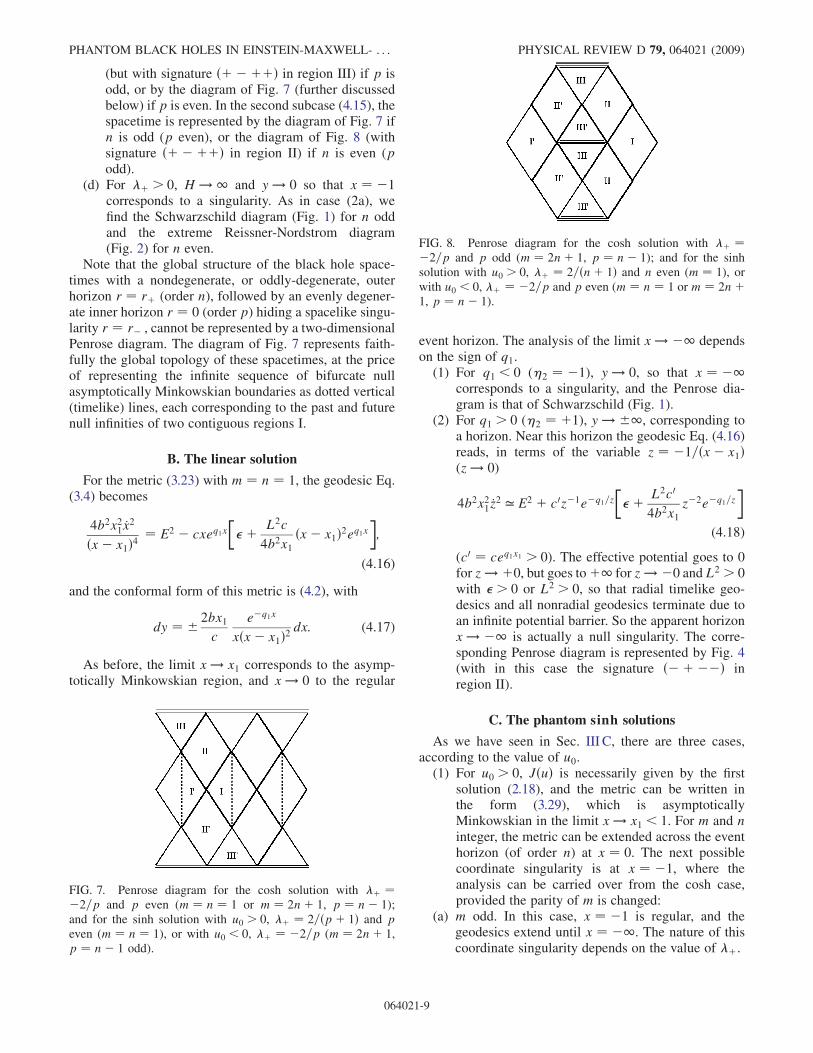
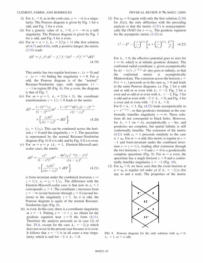
(but with signature ðþ �þþÞ in region III) if p isodd, or by the diagram of Fig. 7 (further discussedbelow) if p is even. In the second subcase (4.15), thespacetime is represented by the diagram of Fig. 7 ifn is odd (p even), or the diagram of Fig. 8 (withsignature ðþ �þþÞ in region II) if n is even (podd).

(d) For �þ > 0, H ! 1 and y ! 0 so that x ¼ �1corresponds to a singularity. As in case (2a), wefind the Schwarzschild diagram (Fig. 1) for n oddand the extreme Reissner-Nordstrom diagram(Fig. 2) for n even.

Note that the global structure of the black hole space-times with a nondegenerate, or oddly-degenerate, outerhorizon r ¼ rþ (order n), followed by an evenly degener-ate inner horizon r ¼ 0 (order p) hiding a spacelike singu-larity r ¼ r� , cannot be represented by a two-dimensionalPenrose diagram. The diagram of Fig. 7 represents faith-fully the global topology of these spacetimes, at the priceof representing the infinite sequence of bifurcate nullasymptotically Minkowskian boundaries as dotted vertical(timelike) lines, each corresponding to the past and futurenull infinities of two contiguous regions I.

B. The linear solution

For the metric (3.23) with m ¼ n ¼ 1, the geodesic Eq.(3.4) becomes

4b2x21 _x2

ðx� x1Þ4¼ E2 � cxeq1x

�þ L2c

4b2x1ðx� x1Þ2eq1x

�;

(4.16)

and the conformal form of this metric is (4.2), with

dy ¼ � 2bx1c

e�q1x

xðx� x1Þ2dx: (4.17)

As before, the limit x ! x1 corresponds to the asymp-totically Minkowskian region, and x ! 0 to the regular

event horizon. The analysis of the limit x ! �1 dependson the sign of q1.(1) For q1 < 0 (�2 ¼ �1), y ! 0, so that x ¼ �1

corresponds to a singularity, and the Penrose dia-gram is that of Schwarzschild (Fig. 1).

(2) For q1 > 0 (�2 ¼ þ1), y ! �1, corresponding toa horizon. Near this horizon the geodesic Eq. (4.16)reads, in terms of the variable z ¼ �1=ðx� x1Þ(z ! 0)

4b2x21 _z2 ’ E2 þ c0z�1e�q1=z

�þ L2c0

4b2x1z�2e�q1=z

�(4.18)

(c0 ¼ ceq1x1 > 0). The effective potential goes to 0for z ! þ0, but goes toþ1 for z ! �0 and L2 > 0with > 0 or L2 > 0, so that radial timelike geo-desics and all nonradial geodesics terminate due toan infinite potential barrier. So the apparent horizonx ! �1 is actually a null singularity. The corre-sponding Penrose diagram is represented by Fig. 4(with in this case the signature ð� þ��Þ inregion II).

C. The phantom sinh solutions

As we have seen in Sec. III C, there are three cases,according to the value of u0.(1) For u0 > 0, JðuÞ is necessarily given by the first

solution (2.18), and the metric can be written inthe form (3.29), which is asymptoticallyMinkowskian in the limit x ! x1 < 1. For m and ninteger, the metric can be extended across the eventhorizon (of order n) at x ¼ 0. The next possiblecoordinate singularity is at x ¼ �1, where theanalysis can be carried over from the cosh case,provided the parity of m is changed:

(a) m odd. In this case, x ¼ �1 is regular, and thegeodesics extend until x ¼ �1. The nature of thiscoordinate singularity depends on the value of �þ.

FIG. 7. Penrose diagram for the cosh solution with �þ ¼�2=p and p even (m ¼ n ¼ 1 or m ¼ 2nþ 1, p ¼ n� 1);and for the sinh solution with u0 > 0, �þ ¼ 2=ðpþ 1Þ and peven (m ¼ n ¼ 1), or with u0 < 0, �þ ¼ �2=p (m ¼ 2nþ 1,p ¼ n� 1 odd).

FIG. 8. Penrose diagram for the cosh solution with �þ ¼�2=p and p odd (m ¼ 2nþ 1, p ¼ n� 1); and for the sinhsolution with u0 > 0, �þ ¼ 2=ðnþ 1Þ and n even (m ¼ 1), orwith u0 < 0, �þ ¼ �2=p and p even (m ¼ n ¼ 1 or m ¼ 2nþ1, p ¼ n� 1).


064021-9

(i) For �þ < 0, as in the cosh case, x ¼ �1 is a singu-larity. The Penrose diagram is given by Fig. 1 for nodd, and Fig. 2 for n even.

(ii) For a generic value of �þ > 0, x ¼ �1 is a nullsingularity. The Penrose diagram is given by Fig. 3for n odd, and Fig. 4 for n even.

(iii) For m ¼ n ¼ 1, �þ ¼ 2=ðpþ 1Þ (the first solutionof (4.7) and (4.8)), with p positive integer, the metric(3.15) reads

dS2 ¼ fþfp�dt2 � f�1þ f�p� dr2 � r2f�pþ1� d�2:

(4.19)

This metric has two regular horizons rþ (x ¼ 0) andr� (x ¼ �1) hiding the singularity r ¼ 0. For podd, the Penrose diagram is of the ‘‘normal’’Reissner-Nordstrom type, with signature ðþ ��Þ in region III (Fig. 6). For p even, the diagramis that of Fig. 7.

(iv) For m ¼ p ¼ 1, �þ ¼ 2=ðnþ 1Þ, the coordinatetransformation x ¼ 1=z < 0 leads to the metric

dS2 ¼ ð�1Þnþ1cz

ð1� zÞnþ1dt2 � ð�1Þnþ14b2z1ð1� zÞnþ1

cðz� z1Þ2

��

z1dx2

zðz� z1Þ2þ d�2

�; (4.20)

(z1 ¼ 1=x1). This can be continued across the hori-zon z ¼ 0 until the singularity z ¼ 1. The spacetimeis represented by the normal Reissner-Nordstromdiagram (Fig. 6) if n is odd, and by Fig. 8 if n is even.

(v) For m ¼ n ¼ p (�þ ¼ 1, Einstein-Maxwell-anti-scalar case), the metric

dS2 ¼ cxn

ð1� xnÞ2 dt2 � 4b2x1x

1�nð1� xnÞ2cðx� x1Þ2

��

x1dx2


�; (4.21)

is form-invariant under the combined inversion x !z ¼ 1=x, x1 ! z1 ¼ 1=x1. The difference with theEinstein-Maxwell-scalar case is that now to x1 < 1corresponds z1 > 1. The coordinate z increases fromz ¼ �1 (event horizon) through z ¼ 0 (second ho-rizon) to the singularity z ¼ 1. As n is odd, thePenrose diagram is again of the normal Reissner-Nordstrom type (Fig. 6).

(b) m even. In this case, there is a coordinate singularityat x ¼ �1. Putting x ¼ �1þ z, we obtain for thegeodesic equation near z ¼ 0 the form (4.11).Therefore the analysis proceeds as in case (2) ofSec. IVA, except for the case �þ ¼ �2=p whichdoes not occur in the present case becausem is even.It follows that x ¼ �1 is in all cases a true singu-larity, which is null for �2 � �þ < 0.

(2) For u0 ¼ 0 (again with only the first solution (2.18)for JðuÞ), the only difference with the precedinganalysis is that the metric (3.31) is nonasymptoti-cally flat (NAF) for x ! x1. The geodesic equationfor the asymptotic metric (3.32) is:

_r 2 � E2 ��r

rþ

�2=�þ

�þ

�r

rþ

�2=�þ L2

r2

�: (4.22)

For �þ < 0, the effective potential goes to zero forr ! 1, which is at infinite geodesic distance. Theconformal radial coordinate y, given asymptotically

by dy� ðr=rþÞ�2=�þdr also goes to infinity, so thatthe conformal metric is asymptoticallyMinkowskian. The extension across the horizon x ¼0 (r ¼ rþ) proceeds as in the case u0 > 0 and leadsto the same Penrose diagrams, i.e. Fig. 1 for n oddand m odd or m even with �þ <�2, Fig. 2 for neven and m odd or m even with �þ <�2, Fig. 3 forn odd andm even with�2 � �þ < 0, and Fig. 4 forn even and m even with �2 � �þ < 0.For 0< �þ < 1, Eq. (4.22) leads asymptotically to

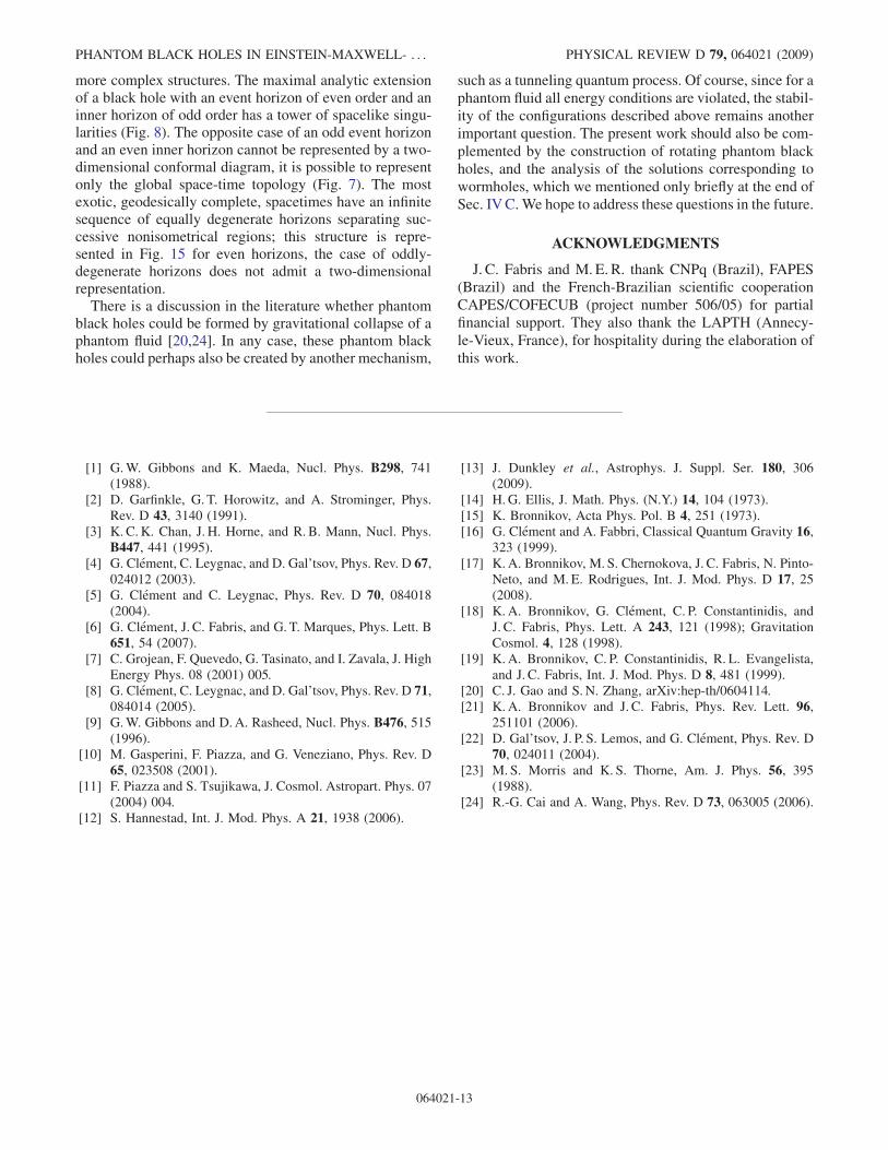
s� r1�1=�þ , so that geodesics terminate at the con-formally timelike singularity r ! 1. These solu-tions do not correspond to black holes. However,for �þ ¼ 1 (m ¼ n), asymptotically s� lnr, andgeodesics are complete, but spatial infinity is stillconformally timelike. The extension of the metric(4.21) with x1 ¼ 1 proceeds similarly to the caseu > u0. Form ¼ n odd, this metric is regular at x ¼�1 and form-invariant under the combined inver-sion x ! z ¼ 1=x, leading after extension throughthe two horizons x ¼ 0 and z ¼ 0 to a geodesicallycomplete spacetime (Fig. 9). For m ¼ n even, thespacetime has a single horizon x ¼ 0 and a confor-mally timelike singularity x ¼ �1 (Fig. 10).

(3) For u0 < 0, we have seen that the event horizon atu ¼ u0 is regular (of order p) if �þ ¼ �2=p (forany m and n real). The properties of the metric

FIG. 9. Penrose diagram for the sinh solution with u0 ¼ 0,�þ ¼ 1, m ¼ n odd.


064021-10

inside the event horizon (u < u0) depend on thesolution (2.18) for JðuÞ.

(a) First solution (2.18). The form of the metric (3.29)shows that x ¼ 0 (u ! �1) is a horizon, which isregular if m and n are positive integers. Because�þ ¼ �2=p, these must satisfy Eq. (4.12). So thereare three possibilities:

(i) For m and n generics, u ¼ �1 is a null singularity.The Penrose diagram is given by Fig. 3 for p odd,and Fig. 4 for p even.

(ii) For m ¼ n ¼ 1, geodesics terminate at the singular-ity x ! �1. The Penrose diagram is given by Fig. 6for p odd, and by Fig. 8 for p even.

(iii) For m ¼ 2nþ 1, p ¼ n� 1, the singularity is againat x ! �1. The Penrose diagram is now given byFig. 7 for p odd, and by Fig. 8 for p even.

(b) Second solution (2.18). The metric is (3.34) withb ¼ 0 and ’1 ¼ �a (which follows from (2.22)),leading to

hðuÞ ¼ ea�u sinhaðu� u0Þ: (4.23)

The associated geodesic equation is

_r 2 ¼ E2 � chp½� L2chp=r2�; (4.24)

with r ¼ �1=u > 0. Near the singularity r ¼ 0

(u ! �1), hðrÞ ’ eð1��Þa=r=2, so that the analysisfollows closely that made in Sec. IVB. Taking intoaccount �2 > 1, there are two possibilities:

(i) If �� > 1, hðrÞ diverges, leading to a spacelikesingularity if p is odd (Fig. 1), or a timelike singu-larity if p is even (Fig. 2).

(ii) If �� <�1, hðrÞ vanishes, signalling a horizon.However the effective potential in (4.24) diverges

for r ! �0 (hðrÞ ’ eð1�Þa=jrj=2), so r ¼ 0 is ac-tually a null singularity. The Penrose diagram isgiven by Fig. 3 if p is odd, and Fig. 4 if p is even.

(c) Third solution (2.18). In (3.34), e2J ¼ �b2=sin2 �bu. Sothe metric has apparent singularities at u ¼ usk k�= �b (k integer). Putting u ¼ usk þ z, the metric

near z ¼ 0 goes to the asymptotically flat form

dS2 ¼ c0dt2 � c0�1ðz�4dz2 þ z�2d�2Þ; (4.25)

with c0 ¼ chpðusÞ. So, in a generic solution sectorusk < u < uskþ1

which does not contain u0, we have

a geodesically complete, horizonless spacetime withtwo asymptotic regions—a Lorentzian wormhole[23] generalizing the � ¼ 0 Bronnikov wormholeof Einstein-Maxwell-anti-scalar theory [15]. In thesolution sector which contains u0, the spacetime isstill geodesically complete with a horizon of orderp. The corresponding Penrose diagrams are given inFig. 11 for p odd, and Fig. 12 for p even.

D. The a ¼ 0 solutions

We have seen in Subsect. III D that there are two regularblack hole cases:(1) For u0 � 0, a ¼ b ¼ 0, the metric is given by (3.37)

with �þ ¼ 2=ðpþ 1Þ. This has a horizon of order(pþ 1) at r ¼ 0 (u ! �1), and a singularity atr ¼ �1=u0. Therefore, for u0 > 0 the Penrose dia-gram is given by Fig. 1 if p is even, and Fig. 2 if p isodd.For u0 ¼ 0, (3.37) is replaced by the nonasymptoti-cally flat metric

dS2 ¼�r

rþ

�pþ1

dt2 ��r

rþ

��ðpþ1Þðdr2 þ r2d�2Þ:(4.26)

The two-dimensional reduced metric is similar tothat of the ‘‘first-class’’ black holes of [16].Spacelike infinity r ! 1 is conformally timelike.For p even, geodesics cross the odd horizon r ¼ 0and terminate at the conformally spacelike singular-ity r ! �1 (Fig. 13). For p odd, r ! �r is an

FIG. 10. Penrose diagram for the sinh solution with u0 ¼ 0,�þ ¼ 1, m ¼ n even.

FIG. 11. Penrose diagram for the sinh solution with u0 < 0(b2 < 0) and �þ ¼ �2=p, p odd.

FIG. 12. Penrose diagram for the sinh solution with u0 < 0(b2 < 0) and �þ ¼ �2=p, p even.


064021-11

isometry of the metric (4.26). The Penrose diagramof these geodesically complete spacetimes is givenin Fig. 14.

(2) For u0 < 0, the metric is (3.34) with hðuÞ given by(3.39). This has a horizon of order p at u ¼ u0 and acoordinate singularity at u ! �1. If b2 > 0 (’1 �0), the metric written in terms of the coordinate xcontains again a nonanalytic logarithm, so that u !�1 (x ¼ 0) is a true singularity. If b2 ¼ 0, themetric reduces to (3.40), which is clearly singularfor u ! �1 (r ¼ 0). In both cases, the Penrosediagram is given by Fig. 1 if p is odd, and Fig. 2if p is even.

E. The sin solution

As seen in Sec. (III E), for this case the only possibilityleading to black holes occurs for the first solution (2.18) forJðuÞ, and is of the form (3.34) with hðuÞ given by (3.42).This can be rewritten as

hðuÞ ¼ e��’1u sin �aðu� usÞ; (4.27)

for us < u < 0, where us ¼ u0 þ k�= �a, with ��= �a <us < 0. The asymptotically Minkowskian (for u ! 0)spacetime therefore presents an infinite series of regularhorizons u ¼ us, u ¼ us � �= �a, u ¼ us � 2�= �a, � � � , allof order p, separating successive regions I, II, and III, � � �which are all different (because of the nonperiodic func-

tions e2JðuÞ and e��’1u). This spacetime is geodesicallycomplete. For p even, the successive regions all have thesame light-cone orientation. The corresponding Penrosediagram is represented in Fig. 15. On the other hand, forp odd, the light-cone orientations alternate between suc-cessive regions, so that geodesics can wind around indef-initely. It is not possible to draw a flat Penrose diagram forthis case.

V. CONCLUSIONS

We have determined in this paper the general static,spherically symmetric solutions for the four-dimensionalEMD theory when the scalar field and/or the electromag-netic field are allowed to violate the null energy condition.The general solution given by (2.17) contains nine classesof asymptotically flat phantom black holes: the ‘‘cosh’’solution, the ‘‘linear’’ solution, the ‘‘sinh’’ solution withu0 > 0, the ‘‘sinh’’ solution with u0 < 0 (three classes), the‘‘a ¼ 0’’ solution with u0 > 0, the ‘‘a ¼ 0’’ solution withu0 < 0, and the ‘‘sin’’ solution. There are also two classesof nonasymptotically flat phantom black holes, corre-sponding to the sinh and the a ¼ 0 solutions with u0 ¼ 0.The event horizon of these black holes can be either

nondegenerate or degenerate. Besides the previouslyknown phantom black holes with a single event horizon[9,20], which occur for generic values of the dilatoniccoupling constant, we have obtained for certain discretevalues of this coupling constant new phantom black holeswith a single event horizon, as well as cold black holes,with a degenerate event horizon. A noteworthy conse-quence of the violation of the null energy condition isthat, for the special case of a vanishing dilaton couplingconstant, there is an infinite sequence of black holes withmultiple event horizons, of the cosh type in the Einstein-anti-Maxwell-anti-scalar case, and of the sinh type in theEinstein-Maxwell-anti-scalar case.We have paid special attention to the study of the causal

structures of these phantom black holes. In total, we havefound 16 different types of causal structures. Many caseslead to Penrose diagrams similar to those of the ‘‘classical’’Schwarzschild, Reissner-Nordstrom, or extreme Reissner-Nordstrom black holes. However, there are new causalstructures. Some of them differ from the preceding bythe fact that the central spacelike or timelike singularityis replaced by a null singularity (Figs. 3 and 4), or that nullinfinity is replaced by timelike infinity (Figs. 10 and 13). Anumber of these spacetimes are geodesically complete withone degenerate horizon (Figs. 11, 12, and 14) or twoequally degenerate horizons (Figs. 5 and 9). We also found

FIG. 13. Penrose diagram for the a ¼ 0 solution (b ¼ 0, u0 ¼0, �þ ¼ 2=ðpþ 1Þ) with p even.

FIG. 14. Penrose diagram for the a ¼ 0 solution (b ¼ 0, u0 ¼0, �þ ¼ 2=ðpþ 1Þ) with p odd.

FIG. 15. Penrose diagram for the sin solution with �þ ¼�2=p, p even.


064021-12

more complex structures. The maximal analytic extensionof a black hole with an event horizon of even order and aninner horizon of odd order has a tower of spacelike singu-larities (Fig. 8). The opposite case of an odd event horizonand an even inner horizon cannot be represented by a two-dimensional conformal diagram, it is possible to representonly the global space-time topology (Fig. 7). The mostexotic, geodesically complete, spacetimes have an infinitesequence of equally degenerate horizons separating suc-cessive nonisometrical regions; this structure is repre-sented in Fig. 15 for even horizons, the case of oddly-degenerate horizons does not admit a two-dimensionalrepresentation.

There is a discussion in the literature whether phantomblack holes could be formed by gravitational collapse of aphantom fluid [20,24]. In any case, these phantom blackholes could perhaps also be created by another mechanism,

such as a tunneling quantum process. Of course, since for aphantom fluid all energy conditions are violated, the stabil-ity of the configurations described above remains anotherimportant question. The present work should also be com-plemented by the construction of rotating phantom blackholes, and the analysis of the solutions corresponding towormholes, which we mentioned only briefly at the end ofSec. IVC.We hope to address these questions in the future.

ACKNOWLEDGMENTS

J. C. Fabris and M. E. R. thank CNPq (Brazil), FAPES(Brazil) and the French-Brazilian scientific cooperationCAPES/COFECUB (project number 506/05) for partialfinancial support. They also thank the LAPTH (Annecy-le-Vieux, France), for hospitality during the elaboration ofthis work.

[1] G.W. Gibbons and K. Maeda, Nucl. Phys. B298, 741(1988).

[2] D. Garfinkle, G. T. Horowitz, and A. Strominger, Phys.Rev. D 43, 3140 (1991).

[3] K. C.K. Chan, J. H. Horne, and R. B. Mann, Nucl. Phys.B447, 441 (1995).

[4] G. Clement, C. Leygnac, and D. Gal’tsov, Phys. Rev. D 67,024012 (2003).

[5] G. Clement and C. Leygnac, Phys. Rev. D 70, 084018(2004).

[6] G. Clement, J. C. Fabris, and G. T. Marques, Phys. Lett. B651, 54 (2007).

[7] C. Grojean, F. Quevedo, G. Tasinato, and I. Zavala, J. HighEnergy Phys. 08 (2001) 005.

[8] G. Clement, C. Leygnac, and D. Gal’tsov, Phys. Rev. D 71,084014 (2005).

[9] G.W. Gibbons and D.A. Rasheed, Nucl. Phys. B476, 515(1996).

[10] M. Gasperini, F. Piazza, and G. Veneziano, Phys. Rev. D65, 023508 (2001).

[11] F. Piazza and S. Tsujikawa, J. Cosmol. Astropart. Phys. 07(2004) 004.

[12] S. Hannestad, Int. J. Mod. Phys. A 21, 1938 (2006).

[13] J. Dunkley et al., Astrophys. J. Suppl. Ser. 180, 306(2009).

[14] H. G. Ellis, J. Math. Phys. (N.Y.) 14, 104 (1973).[15] K. Bronnikov, Acta Phys. Pol. B 4, 251 (1973).[16] G. Clement and A. Fabbri, Classical Quantum Gravity 16,

323 (1999).[17] K. A. Bronnikov, M. S. Chernokova, J. C. Fabris, N. Pinto-

Neto, and M. E. Rodrigues, Int. J. Mod. Phys. D 17, 25(2008).

[18] K. A. Bronnikov, G. Clement, C. P. Constantinidis, andJ. C. Fabris, Phys. Lett. A 243, 121 (1998); GravitationCosmol. 4, 128 (1998).

[19] K. A. Bronnikov, C. P. Constantinidis, R. L. Evangelista,and J. C. Fabris, Int. J. Mod. Phys. D 8, 481 (1999).

[20] C. J. Gao and S.N. Zhang, arXiv:hep-th/0604114.[21] K. A. Bronnikov and J. C. Fabris, Phys. Rev. Lett. 96,

251101 (2006).[22] D. Gal’tsov, J. P. S. Lemos, and G. Clement, Phys. Rev. D

70, 024011 (2004).[23] M. S. Morris and K. S. Thorne, Am. J. Phys. 56, 395

(1988).[24] R.-G. Cai and A. Wang, Phys. Rev. D 73, 063005 (2006).


064021-13

Documents

Phantom black holes in Einstein-Maxwell-dilaton theory