Embed Size (px)
Citation preview
ANL-95/11
PETSc Users ManualRevision 3.2
byS. Balay, J. Brown, K. Buschelman, V. Eijkhout, W. Gropp, D. Kaushik,M. Knepley, L. Curfman McInnes, B. Smith, and H. ZhangMathematics and Computer Science Division, Argonne National Laboratory
Sept 2011
This work was supported by the Office of Advanced Scientific Computing Research,Office of Science, U.S. Department of Energy, under Contract DE-AC02-06CH11357.
1
Availability of This Report
This report is available, at no cost, at http://www.osti.gov/bridge. It is also available on paper to the U.S. Department of Energy and its contractors, for a processing fee, from: U.S. Department of Energy Office of Scientific and Technical Information
P.O. Box 62 Oak Ridge, TN 37831-0062 phone (865) 576-8401 fax (865) 576-5728 [email protected]
Disclaimer
This report was prepared as an account of work sponsored by an agency of the United States Government. Neither the United States Government nor any agency thereof, nor UChicago Argonne, LLC, nor any of their employees or officers, makes any warranty, express
or implied, or assumes any legal liability or responsibility for the accuracy, completeness, or usefulness of any information, apparatus, product, or process disclosed, or represents that its use would not infringe privately owned rights. Reference herein to any specific commercial product, process, or service by trade name, trademark, manufacturer, or otherwise, does not necessarily constitute or imply its endorsement, recommendation, or favoring by the United States Government or any agency thereof. The views and opinions of document authors expressed herein do not necessarily state or reflect those of the United States Government or any agency thereof,
Argonne National Laboratory, or UChicago Argonne, LLC.
About Argonne National Laboratory
Argonne is a U.S. Department of Energy laboratory managed by UChicago Argonne, LLC under contract DE-AC02-06CH11357. The Laboratory’s main facility is outside Chicago, at 9700 South Cass Avenue, Argonne, Illinois 60439. For information about Argonne and its pioneering science and technology programs, see www.anl.gov.
Figure 1:
2
Abstract:
This manual describes the use of PETSc for the numerical solution of partial differential equations andrelated problems on high-performance computers. The Portable, Extensible Toolkit for Scientific Compu-tation (PETSc) is a suite of data structures and routines that provide the building blocks for the implemen-tation of large-scale application codes on parallel (and serial) computers. PETSc uses the MPI standard forall message-passing communication.
PETSc includes an expanding suite of parallel linear, nonlinear equation solvers and time integratorsthat may be used in application codes written in Fortran, C, C++, Python, and MATLAB (sequential).PETSc provides many of the mechanisms needed within parallel application codes, such as parallel matrixand vector assembly routines. The library is organized hierarchically, enabling users to employ the levelof abstraction that is most appropriate for a particular problem. By using techniques of object-orientedprogramming, PETSc provides enormous flexibility for users.
PETSc is a sophisticated set of software tools; as such, for some users it initially has a much steeperlearning curve than a simple subroutine library. In particular, for individuals without some computer sciencebackground, experience programming in C, C++ or Fortran and experience using a debugger such as gdbor dbx, it may require a significant amount of time to take full advantage of the features that enable efficientsoftware use. However, the power of the PETSc design and the algorithms it incorporates may make theefficient implementation of many application codes simpler than “rolling them” yourself.
• For many tasks a package such as MATLAB is often the best tool; PETSc is not intended for theclasses of problems for which effective MATLAB code can be written. PETSc also has a MATLABinterface, so portions of your code can be written in MATLAB to “try out” the PETSc solvers. Theresulting code will not be scalable however because currently MATLAB is inherently not scalable.
• PETSc should not be used to attempt to provide a “parallel linear solver” in an otherwise sequentialcode. Certainly all parts of a previously sequential code need not be parallelized but the matrixgeneration portion must be parallelized to expect any kind of reasonable performance. Do not expectto generate your matrix sequentially and then “use PETSc” to solve the linear system in parallel.
Since PETSc is under continued development, small changes in usage and calling sequences of routineswill occur. PETSc is supported; see the web site http://www.mcs.anl.gov/petsc for information on contactingsupport.
A http://www.mcs.anl.gov/petsc/petsc-as/publications may be found a list of publications and web sitesthat feature work involving PETSc.
We welcome any reports of corrections for this document.
3

4
Getting Information on PETSc:
On-line:• Manual pages–example usage docs/index.html or http://www.mcs.anl.gov/petsc/petsc-as/documentation
• Installing PETSc http://www.mcs.anl.gov/petsc/petsc-as/documentation/installation.html
In this manual:• Basic introduction, page 19
• Assembling vectors, page 43; and matrices, 57
• Linear solvers, page 71
• Nonlinear solvers, page 91
• Timestepping (ODE) solvers, page 115
• Index, page 197
5

6

Acknowledgments:
We thank all PETSc users for their many suggestions, bug reports, and encouragement. We especially thankDavid Keyes for his valuable comments on the source code, functionality, and documentation for PETSc.
Some of the source code and utilities in PETSc have been written by
• Asbjorn Hoiland Aarrestad - the explicit Runge-Kutta implementations;
• Mark Adams - scalability features of MPIBAIJ matrices;
• G. Anciaux and J. Roman - the interfaces to the partitioning packages PTScotch, Chaco, and Party;
• Allison Baker - the flexible GMRES code and LGMRES;
• Chad Carroll - Win32 graphics;
• Ethan Coon - the PetscBag and many bug fixes;
• Cameron Cooper - portions of the VecScatter routines;
• Paulo Goldfeld - balancing Neumann-Neumann preconditioner;
• Matt Hille;
• Joel Malard - the BICGStab(l) implementation;
• Paul Mullowney, enhancements to portions of the Nvidia GPU interface;
• Dave May - the GCR implementation
• Peter Mell - portions of the DA routines;
• Richard Mills - the AIJPERM matrix format for the Cray X1 and universal F90 array interface;
• Victor Minden - the NVidia GPU interface;
• Todd Munson - the LUSOL (sparse solver in MINOS) interface and several Krylov methods;
• Adam Powell - the PETSc Debian package,
• Robert Scheichl - the MINRES implementation,
• Kerry Stevens - the pthread based Vec and Mat classes plus the various thread pools
• Karen Toonen - designed and implemented much of the PETSc web pages,
• Desire Nuentsa Wakam - the deflated GMRES implementation,
• Liyang Xu - the interface to PVODE (now Sundials/CVODE).
PETSc uses routines from
• BLAS;
• LAPACK;
7
• LINPACK - dense matrix factorization and solve; converted to C using f2c and then hand-optimizedfor small matrix sizes, for block matrix data structures;
• MINPACK - see page 111, sequential matrix coloring routines for finite difference Jacobian evalua-tions; converted to C using f2c;
• SPARSPAK - see page 79, matrix reordering routines, converted to C using f2c;
• libtfs - the efficient, parallel direct solver developed by Henry Tufo and Paul Fischer for the directsolution of a coarse grid problem (a linear system with very few degrees of freedom per processor).
PETSc interfaces to the following external software:
• ADIC/ADIFOR - automatic differentiation for the computation of sparse Jacobians,http://www.mcs.anl.gov/adic, http://www.mcs.anl.gov/adifor,
• Chaco - A graph partitioning package, http://www.cs.sandia.gov/CRF/chac.html
• ESSL - IBM’s math library for fast sparse direct LU factorization,
• Euclid - parallel ILU(k) developed by David Hysom, accessed through the Hypre interface,
• Hypre - the LLNL preconditioner library, http://www.llnl.gov/CASC/hypre
• LUSOL - sparse LU factorization code (part of MINOS) developed by Michael Saunders, SystemsOptimization Laboratory, Stanford University, http://www.sbsi-sol-optimize.com/,
• Mathematica - see page ??,
• MATLAB - see page 127,
• MUMPS - see page 88, MUltifrontal Massively Parallel sparse direct Solver developed by PatrickAmestoy, Iain Duff, Jacko Koster, and Jean-Yves L’Excellent,http://www.enseeiht.fr/lima/apo/MUMPS/credits.html,
• ParMeTiS - see page 68, parallel graph partitioner, http://www-users.cs.umn.edu/ karypis/metis/,
• Party - A graph partitioning package,http://www.uni-paderborn.de/fachbereich/AG/monien/RESEARCH/PART/party.html,
• PaStiX - Parallel LU and Cholesky solvers,
• Prometheus - Scalable unstructured finite element solver http://www.columbia.edu/ ma2325/prometheus/,
• PLAPACK - Parallel Linear Algebra Package, http://www.cs.utexas.edu/users/plapack/,
• PTScotch - A graph partitioning package, http://www.labri.fr/Perso/ pelegrin/scotch/
• SPAI - for parallel sparse approximate inverse preconditiong, http://www.sam.math.ethz.ch/ grote/s-pai/,
• SPOOLES - see page 88, SParse Object Oriented Linear Equations Solver, developed by CleveAshcraft, http://www.netlib.org/linalg/spooles/spooles.2.2.html,
• Sundial/CVODE - see page 119, parallel ODE integrator, http://www.llnl.gov/CASC/sundials/,
8

• SuperLU and SuperLU Dist - see page 88, the efficient sparse LU codes developed by Jim Demmel,Xiaoye S. Li, and John Gilbert, http://www.nersc.gov/ xiaoye/SuperLU,
• Trilinos/ML - Sandia’s main multigrid preconditioning package, http://software.sandia.gov/trilinos/,
• UMFPACK - see page 88, developed by Timothy A. Davis, http://www.cise.ufl.edu/research/sparse/umfpack/.
These are all optional packages and do not need to be installed to use PETSc.PETSc software is developed and maintained with
• Mecurial revision control system
• Emacs editor
PETSc documentation has been generated using
• the text processing tools developed by Bill Gropp
• c2html
• pdflatex
• python
9

10
Contents
Abstract 3
I Introduction to PETSc 17
1 Getting Started 191.1 Suggested Reading . . . . . . . . . . . . . . . . . . . . . . . . . . . . . . . . . . . . . . . 201.2 Running PETSc Programs . . . . . . . . . . . . . . . . . . . . . . . . . . . . . . . . . . . 221.3 Writing PETSc Programs . . . . . . . . . . . . . . . . . . . . . . . . . . . . . . . . . . . . 231.4 Simple PETSc Examples . . . . . . . . . . . . . . . . . . . . . . . . . . . . . . . . . . . . 241.5 Referencing PETSc . . . . . . . . . . . . . . . . . . . . . . . . . . . . . . . . . . . . . . . 361.6 Directory Structure . . . . . . . . . . . . . . . . . . . . . . . . . . . . . . . . . . . . . . . 36
II Programming with PETSc 39
2 Vectors and Distributing Parallel Data 412.1 Creating and Assembling Vectors . . . . . . . . . . . . . . . . . . . . . . . . . . . . . . . . 412.2 Basic Vector Operations . . . . . . . . . . . . . . . . . . . . . . . . . . . . . . . . . . . . 432.3 Indexing and Ordering . . . . . . . . . . . . . . . . . . . . . . . . . . . . . . . . . . . . . 45
2.3.1 Application Orderings . . . . . . . . . . . . . . . . . . . . . . . . . . . . . . . . . 452.3.2 Local to Global Mappings . . . . . . . . . . . . . . . . . . . . . . . . . . . . . . . 46
2.4 Structured Grids Using Distributed Arrays . . . . . . . . . . . . . . . . . . . . . . . . . . . 472.4.1 Creating Distributed Arrays . . . . . . . . . . . . . . . . . . . . . . . . . . . . . . 482.4.2 Local/Global Vectors and Scatters . . . . . . . . . . . . . . . . . . . . . . . . . . . 492.4.3 Local (Ghosted) Work Vectors . . . . . . . . . . . . . . . . . . . . . . . . . . . . . 502.4.4 Accessing the Vector Entries for DMDA Vectors . . . . . . . . . . . . . . . . . . . 502.4.5 Grid Information . . . . . . . . . . . . . . . . . . . . . . . . . . . . . . . . . . . . 51
2.5 Software for Managing Vectors Related to Unstructured Grids . . . . . . . . . . . . . . . . 522.5.1 Index Sets . . . . . . . . . . . . . . . . . . . . . . . . . . . . . . . . . . . . . . . . 522.5.2 Scatters and Gathers . . . . . . . . . . . . . . . . . . . . . . . . . . . . . . . . . . 532.5.3 Scattering Ghost Values . . . . . . . . . . . . . . . . . . . . . . . . . . . . . . . . 542.5.4 Vectors with Locations for Ghost Values . . . . . . . . . . . . . . . . . . . . . . . . 55
3 Matrices 573.1 Creating and Assembling Matrices . . . . . . . . . . . . . . . . . . . . . . . . . . . . . . . 57
3.1.1 Sparse Matrices . . . . . . . . . . . . . . . . . . . . . . . . . . . . . . . . . . . . . 583.1.2 Dense Matrices . . . . . . . . . . . . . . . . . . . . . . . . . . . . . . . . . . . . . 623.1.3 Block Matrices . . . . . . . . . . . . . . . . . . . . . . . . . . . . . . . . . . . . . 63
11
3.2 Basic Matrix Operations . . . . . . . . . . . . . . . . . . . . . . . . . . . . . . . . . . . . 653.3 Matrix-Free Matrices . . . . . . . . . . . . . . . . . . . . . . . . . . . . . . . . . . . . . . 653.4 Other Matrix Operations . . . . . . . . . . . . . . . . . . . . . . . . . . . . . . . . . . . . 673.5 Partitioning . . . . . . . . . . . . . . . . . . . . . . . . . . . . . . . . . . . . . . . . . . . 68
4 KSP: Linear Equations Solvers 714.1 Using KSP . . . . . . . . . . . . . . . . . . . . . . . . . . . . . . . . . . . . . . . . . . . 714.2 Solving Successive Linear Systems . . . . . . . . . . . . . . . . . . . . . . . . . . . . . . . 734.3 Krylov Methods . . . . . . . . . . . . . . . . . . . . . . . . . . . . . . . . . . . . . . . . . 73
4.3.1 Preconditioning within KSP . . . . . . . . . . . . . . . . . . . . . . . . . . . . . . 744.3.2 Convergence Tests . . . . . . . . . . . . . . . . . . . . . . . . . . . . . . . . . . . 754.3.3 Convergence Monitoring . . . . . . . . . . . . . . . . . . . . . . . . . . . . . . . . 764.3.4 Understanding the Operator’s Spectrum . . . . . . . . . . . . . . . . . . . . . . . . 774.3.5 Other KSP Options . . . . . . . . . . . . . . . . . . . . . . . . . . . . . . . . . . . 77
4.4 Preconditioners . . . . . . . . . . . . . . . . . . . . . . . . . . . . . . . . . . . . . . . . . 784.4.1 ILU and ICC Preconditioners . . . . . . . . . . . . . . . . . . . . . . . . . . . . . 784.4.2 SOR and SSOR Preconditioners . . . . . . . . . . . . . . . . . . . . . . . . . . . . 794.4.3 LU Factorization . . . . . . . . . . . . . . . . . . . . . . . . . . . . . . . . . . . . 794.4.4 Block Jacobi and Overlapping Additive Schwarz Preconditioners . . . . . . . . . . 804.4.5 Shell Preconditioners . . . . . . . . . . . . . . . . . . . . . . . . . . . . . . . . . . 814.4.6 Combining Preconditioners . . . . . . . . . . . . . . . . . . . . . . . . . . . . . . 824.4.7 Multigrid Preconditioners . . . . . . . . . . . . . . . . . . . . . . . . . . . . . . . 83
4.5 Solving Block Matrices . . . . . . . . . . . . . . . . . . . . . . . . . . . . . . . . . . . . . 854.6 Solving Singular Systems . . . . . . . . . . . . . . . . . . . . . . . . . . . . . . . . . . . . 884.7 Using PETSc to interface with external linear solvers . . . . . . . . . . . . . . . . . . . . . 88
5 SNES: Nonlinear Solvers 915.1 Basic SNES Usage . . . . . . . . . . . . . . . . . . . . . . . . . . . . . . . . . . . . . . . 91
5.1.1 Nonlinear Function Evaluation . . . . . . . . . . . . . . . . . . . . . . . . . . . . . 995.1.2 Jacobian Evaluation . . . . . . . . . . . . . . . . . . . . . . . . . . . . . . . . . . 99
5.2 The Nonlinear Solvers . . . . . . . . . . . . . . . . . . . . . . . . . . . . . . . . . . . . . 1005.2.1 Line Search Techniques . . . . . . . . . . . . . . . . . . . . . . . . . . . . . . . . 1005.2.2 Trust Region Methods . . . . . . . . . . . . . . . . . . . . . . . . . . . . . . . . . 101
5.3 General Options . . . . . . . . . . . . . . . . . . . . . . . . . . . . . . . . . . . . . . . . . 1015.3.1 Convergence Tests . . . . . . . . . . . . . . . . . . . . . . . . . . . . . . . . . . . 1015.3.2 Convergence Monitoring . . . . . . . . . . . . . . . . . . . . . . . . . . . . . . . . 1025.3.3 Checking Accuracy of Derivatives . . . . . . . . . . . . . . . . . . . . . . . . . . . 102
5.4 Inexact Newton-like Methods . . . . . . . . . . . . . . . . . . . . . . . . . . . . . . . . . . 1035.5 Matrix-Free Methods . . . . . . . . . . . . . . . . . . . . . . . . . . . . . . . . . . . . . . 1035.6 Finite Difference Jacobian Approximations . . . . . . . . . . . . . . . . . . . . . . . . . . 1115.7 Variational Inequalities . . . . . . . . . . . . . . . . . . . . . . . . . . . . . . . . . . . . . 113
6 TS: Scalable ODE and DAE Solvers 1156.1 Basic TS Usage . . . . . . . . . . . . . . . . . . . . . . . . . . . . . . . . . . . . . . . . . 116
6.1.1 Solving Time-dependent Problems . . . . . . . . . . . . . . . . . . . . . . . . . . . 1176.1.2 Solving Differential Algebraic Equations . . . . . . . . . . . . . . . . . . . . . . . 1186.1.3 Using Implicit-Explicit (IMEX) methods for multi-rate problems . . . . . . . . . . . 1196.1.4 Using Sundials from PETSc . . . . . . . . . . . . . . . . . . . . . . . . . . . . . . 1196.1.5 Solving Steady-State Problems with Pseudo-Timestepping . . . . . . . . . . . . . . 120
12
6.1.6 Using the Explicit Runge-Kutta timestepper with variable timesteps . . . . . . . . . 121
7 High Level Support for Multigrid with DMMG 123
8 Using ADIC and ADIFOR with PETSc 1258.1 Work arrays inside the local functions . . . . . . . . . . . . . . . . . . . . . . . . . . . . . 125
9 Using MATLAB with PETSc 1279.1 Dumping Data for MATLAB . . . . . . . . . . . . . . . . . . . . . . . . . . . . . . . . . . 1279.2 Sending Data to Interactive Running MATLAB Session . . . . . . . . . . . . . . . . . . . . 1279.3 Using the MATLAB Compute Engine . . . . . . . . . . . . . . . . . . . . . . . . . . . . . 1289.4 Using PETSc objects directly in MATLAB . . . . . . . . . . . . . . . . . . . . . . . . . . . 129
10 PETSc for Fortran Users 13110.1 Differences between PETSc Interfaces for C and Fortran . . . . . . . . . . . . . . . . . . . 131
10.1.1 Include Files . . . . . . . . . . . . . . . . . . . . . . . . . . . . . . . . . . . . . . 13110.1.2 Error Checking . . . . . . . . . . . . . . . . . . . . . . . . . . . . . . . . . . . . . 13210.1.3 Array Arguments . . . . . . . . . . . . . . . . . . . . . . . . . . . . . . . . . . . . 13210.1.4 Calling Fortran Routines from C (and C Routines from Fortran) . . . . . . . . . . . 13310.1.5 Passing Null Pointers . . . . . . . . . . . . . . . . . . . . . . . . . . . . . . . . . . 13310.1.6 Duplicating Multiple Vectors . . . . . . . . . . . . . . . . . . . . . . . . . . . . . . 13410.1.7 Matrix, Vector and IS Indices . . . . . . . . . . . . . . . . . . . . . . . . . . . . . 13410.1.8 Setting Routines . . . . . . . . . . . . . . . . . . . . . . . . . . . . . . . . . . . . 13410.1.9 Compiling and Linking Fortran Programs . . . . . . . . . . . . . . . . . . . . . . . 13410.1.10 Routines with Different Fortran Interfaces . . . . . . . . . . . . . . . . . . . . . . . 13510.1.11 Fortran90 . . . . . . . . . . . . . . . . . . . . . . . . . . . . . . . . . . . . . . . . 135
10.2 Sample Fortran77 Programs . . . . . . . . . . . . . . . . . . . . . . . . . . . . . . . . . . 135
III Additional Information 149
11 Profiling 15111.1 Basic Profiling Information . . . . . . . . . . . . . . . . . . . . . . . . . . . . . . . . . . . 151
11.1.1 Interpreting -log summary Output: The Basics . . . . . . . . . . . . . . . . . . . 15111.1.2 Interpreting -log summary Output: Parallel Performance . . . . . . . . . . . . . 15211.1.3 Using -log mpe with Upshot/Jumpshot . . . . . . . . . . . . . . . . . . . . . . . 154
11.2 Profiling Application Codes . . . . . . . . . . . . . . . . . . . . . . . . . . . . . . . . . . 15511.3 Profiling Multiple Sections of Code . . . . . . . . . . . . . . . . . . . . . . . . . . . . . . 15611.4 Restricting Event Logging . . . . . . . . . . . . . . . . . . . . . . . . . . . . . . . . . . . 15711.5 Interpreting -log info Output: Informative Messages . . . . . . . . . . . . . . . . . . . 15711.6 Time . . . . . . . . . . . . . . . . . . . . . . . . . . . . . . . . . . . . . . . . . . . . . . . 15811.7 Saving Output to a File . . . . . . . . . . . . . . . . . . . . . . . . . . . . . . . . . . . . . 15811.8 Accurate Profiling: Overcoming the Overhead of Paging . . . . . . . . . . . . . . . . . . . 158
12 Hints for Performance Tuning 16112.1 Compiler Options . . . . . . . . . . . . . . . . . . . . . . . . . . . . . . . . . . . . . . . . 16112.2 Profiling . . . . . . . . . . . . . . . . . . . . . . . . . . . . . . . . . . . . . . . . . . . . . 16112.3 Aggregation . . . . . . . . . . . . . . . . . . . . . . . . . . . . . . . . . . . . . . . . . . . 16112.4 Efficient Memory Allocation . . . . . . . . . . . . . . . . . . . . . . . . . . . . . . . . . . 162
12.4.1 Sparse Matrix Assembly . . . . . . . . . . . . . . . . . . . . . . . . . . . . . . . . 162
13
12.4.2 Sparse Matrix Factorization . . . . . . . . . . . . . . . . . . . . . . . . . . . . . . 16212.4.3 PetscMalloc() Calls . . . . . . . . . . . . . . . . . . . . . . . . . . . . . . . . . . . 162
12.5 Data Structure Reuse . . . . . . . . . . . . . . . . . . . . . . . . . . . . . . . . . . . . . . 16212.6 Numerical Experiments . . . . . . . . . . . . . . . . . . . . . . . . . . . . . . . . . . . . . 16312.7 Tips for Efficient Use of Linear Solvers . . . . . . . . . . . . . . . . . . . . . . . . . . . . 16312.8 Detecting Memory Allocation Problems . . . . . . . . . . . . . . . . . . . . . . . . . . . . 16312.9 System-Related Problems . . . . . . . . . . . . . . . . . . . . . . . . . . . . . . . . . . . . 164
13 Other PETSc Features 16713.1 PETSc on a process subset . . . . . . . . . . . . . . . . . . . . . . . . . . . . . . . . . . . 16713.2 Runtime Options . . . . . . . . . . . . . . . . . . . . . . . . . . . . . . . . . . . . . . . . 167
13.2.1 The Options Database . . . . . . . . . . . . . . . . . . . . . . . . . . . . . . . . . 16713.2.2 User-Defined PetscOptions . . . . . . . . . . . . . . . . . . . . . . . . . . . . . . . 16813.2.3 Keeping Track of Options . . . . . . . . . . . . . . . . . . . . . . . . . . . . . . . 169
13.3 Viewers: Looking at PETSc Objects . . . . . . . . . . . . . . . . . . . . . . . . . . . . . . 16913.4 Debugging . . . . . . . . . . . . . . . . . . . . . . . . . . . . . . . . . . . . . . . . . . . . 17013.5 Error Handling . . . . . . . . . . . . . . . . . . . . . . . . . . . . . . . . . . . . . . . . . 17113.6 Incremental Debugging . . . . . . . . . . . . . . . . . . . . . . . . . . . . . . . . . . . . . 17213.7 Complex Numbers . . . . . . . . . . . . . . . . . . . . . . . . . . . . . . . . . . . . . . . 17313.8 Emacs Users . . . . . . . . . . . . . . . . . . . . . . . . . . . . . . . . . . . . . . . . . . . 17413.9 Vi and Vim Users . . . . . . . . . . . . . . . . . . . . . . . . . . . . . . . . . . . . . . . . 17413.10Eclipse Users . . . . . . . . . . . . . . . . . . . . . . . . . . . . . . . . . . . . . . . . . . 17513.11Qt Creator . . . . . . . . . . . . . . . . . . . . . . . . . . . . . . . . . . . . . . . . . . . . 17513.12Developers Studio Users . . . . . . . . . . . . . . . . . . . . . . . . . . . . . . . . . . . . 17713.13XCode Users (The Apple GUI Development System . . . . . . . . . . . . . . . . . . . . . 17713.14Parallel Communication . . . . . . . . . . . . . . . . . . . . . . . . . . . . . . . . . . . . 17713.15Graphics . . . . . . . . . . . . . . . . . . . . . . . . . . . . . . . . . . . . . . . . . . . . . 178
13.15.1 Windows as PetscViewers . . . . . . . . . . . . . . . . . . . . . . . . . . . . . . . 17813.15.2 Simple PetscDrawing . . . . . . . . . . . . . . . . . . . . . . . . . . . . . . . . . . 17813.15.3 Line Graphs . . . . . . . . . . . . . . . . . . . . . . . . . . . . . . . . . . . . . . . 17913.15.4 Graphical Convergence Monitor . . . . . . . . . . . . . . . . . . . . . . . . . . . . 18113.15.5 Disabling Graphics at Compile Time . . . . . . . . . . . . . . . . . . . . . . . . . . 181
14 Makefiles 18314.1 Our Makefile System . . . . . . . . . . . . . . . . . . . . . . . . . . . . . . . . . . . . . . 183
14.1.1 Makefile Commands . . . . . . . . . . . . . . . . . . . . . . . . . . . . . . . . . . 18314.1.2 Customized Makefiles . . . . . . . . . . . . . . . . . . . . . . . . . . . . . . . . . 184
14.2 PETSc Flags . . . . . . . . . . . . . . . . . . . . . . . . . . . . . . . . . . . . . . . . . . . 18414.2.1 Sample Makefiles . . . . . . . . . . . . . . . . . . . . . . . . . . . . . . . . . . . . 184
14.3 Limitations . . . . . . . . . . . . . . . . . . . . . . . . . . . . . . . . . . . . . . . . . . . 187
15 Unimportant and Advanced Features of Matrices and Solvers 18915.1 Extracting Submatrices . . . . . . . . . . . . . . . . . . . . . . . . . . . . . . . . . . . . . 18915.2 Matrix Factorization . . . . . . . . . . . . . . . . . . . . . . . . . . . . . . . . . . . . . . 18915.3 Unimportant Details of KSP . . . . . . . . . . . . . . . . . . . . . . . . . . . . . . . . . . 19115.4 Unimportant Details of PC . . . . . . . . . . . . . . . . . . . . . . . . . . . . . . . . . . . 192
14

16 Unstructured Grids in PETSc 19516.1 Sections: Vectors on Unstructured Grids . . . . . . . . . . . . . . . . . . . . . . . . . . . . 195
16.1.1 Defining Sections . . . . . . . . . . . . . . . . . . . . . . . . . . . . . . . . . . . . 19516.1.2 Updating Values . . . . . . . . . . . . . . . . . . . . . . . . . . . . . . . . . . . . 196
Index 197
Bibliography 209
15

16
Part I
Introduction to PETSc
17

Chapter 1
Getting Started
The Portable, Extensible Toolkit for Scientific Computation (PETSc) has successfully demonstrated that theuse of modern programming paradigms can ease the development of large-scale scientific application codesin Fortran, C, C++, and Pyton. Begun several years ago, the software has evolved into a powerful set oftools for the numerical solution of partial differential equations and related problems on high-performancecomputers. PETSc is also callable directly from MATLAB (sequential) to allow “trying out” PETSc’ssolvers from prototype MATLAB code.
PETSc consists of a variety of libraries (similar to classes in C++), which are discussed in detail inParts II and III of the users manual. Each library manipulates a particular family of objects (for instance,vectors) and the operations one would like to perform on the objects. The objects and operations in PETScare derived from our long experiences with scientific computation. Some of the PETSc modules deal with
• index sets (IS), including permutations, for indexing into vectors, renumbering, etc;
• vectors (Vec);
• matrices (Mat) (generally sparse);
• managing interactions between mesh data structures and vectors and matrices (DM);
• over fifteen Krylov subspace methods (KSP);
• dozens of preconditioners, including multigrid, block solvers, and sparse direct solvers (PC);
• nonlinear solvers (SNES); and
• timesteppers for solving time-dependent (nonlinear) PDEs, including support for differential algebraicequations (TS).
Each consists of an abstract interface (simply a set of calling sequences) and one or more implementationsusing particular data structures. Thus, PETSc provides clean and effective codes for the various phasesof solving PDEs, with a uniform approach for each class of problems. This design enables easy compar-ison and use of different algorithms (for example, to experiment with different Krylov subspace methods,preconditioners, or truncated Newton methods). Hence, PETSc provides a rich environment for modelingscientific applications as well as for rapid algorithm design and prototyping.
The libraries enable easy customization and extension of both algorithms and implementations. Thisapproach promotes code reuse and flexibility, and separates the issues of parallelism from the choice ofalgorithms. The PETSc infrastructure creates a foundation for building large-scale applications.
It is useful to consider the interrelationships among different pieces of PETSc. Figure 2 is a diagram ofsome of these pieces; Figure 3 presents several of the individual parts in more detail. These figures illustrate
19
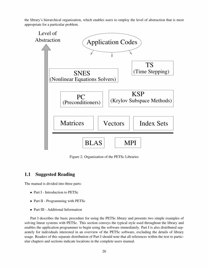
the library’s hierarchical organization, which enables users to employ the level of abstraction that is mostappropriate for a particular problem.
Matrices Vectors Index Sets
Level of
Abstraction Application Codes
BLAS
SNES
MPI
KSP(Krylov Subspace Methods)
TS(Time Stepping)
(Nonlinear Equations Solvers)
(Preconditioners)PC
Figure 2: Organization of the PETSc Libraries
1.1 Suggested Reading
The manual is divided into three parts:
• Part I - Introduction to PETSc
• Part II - Programming with PETSc
• Part III - Additional Information
Part I describes the basic procedure for using the PETSc library and presents two simple examples ofsolving linear systems with PETSc. This section conveys the typical style used throughout the library andenables the application programmer to begin using the software immediately. Part I is also distributed sep-arately for individuals interested in an overview of the PETSc software, excluding the details of libraryusage. Readers of this separate distribution of Part I should note that all references within the text to partic-ular chapters and sections indicate locations in the complete users manual.
20
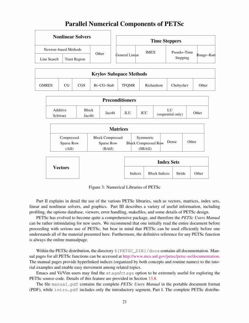
Krylov Subspace Methods
CG CGS OtherChebychevRichardsonTFQMRBi−CG−StabGMRES
VectorsOtherStrideBlock Indices
Index Sets
Indices
Block Compressed
Sparse Row
(BAIJ)
Symmetric
Block Compressed Row
(SBAIJ)
Compressed
Sparse Row
(AIJ)
OtherDense
Matrices
IMEX Pseudo−Time
Stepping
Time Steppers
General Linear Runge−Kutta
Block
Jacobi
Additive
Schwarz (sequential only)LU
Parallel Numerical Components of PETSc
Jacobi ILU ICC Other
Preconditioners
Newton−based Methods
Trust RegionLine Search
Other
Nonlinear Solvers
Figure 3: Numerical Libraries of PETSc
Part II explains in detail the use of the various PETSc libraries, such as vectors, matrices, index sets,linear and nonlinear solvers, and graphics. Part III describes a variety of useful information, includingprofiling, the options database, viewers, error handling, makefiles, and some details of PETSc design.
PETSc has evolved to become quite a comprehensive package, and therefore the PETSc Users Manualcan be rather intimidating for new users. We recommend that one initially read the entire document beforeproceeding with serious use of PETSc, but bear in mind that PETSc can be used efficiently before oneunderstands all of the material presented here. Furthermore, the definitive reference for any PETSc functionis always the online manualpage.
Within the PETSc distribution, the directory ${PETSC_DIR}/docs contains all documentation. Man-ual pages for all PETSc functions can be accessed at http://www.mcs.anl.gov/petsc/petsc-as/documentation.The manual pages provide hyperlinked indices (organized by both concepts and routine names) to the tuto-rial examples and enable easy movement among related topics.
Emacs and Vi/Vim users may find the etags/ctags option to be extremely useful for exploring thePETSc source code. Details of this feature are provided in Section 13.8.
The file manual.pdf contains the complete PETSc Users Manual in the portable document format(PDF), while intro.pdf includes only the introductory segment, Part I. The complete PETSc distribu-
21
tion, users manual, manual pages, and additional information are also available via the PETSc home pageat http://www.mcs.anl.gov/petsc. The PETSc home page also contains details regarding installation, newfeatures and changes in recent versions of PETSc, machines that we currently support, and a FAQ list forfrequently asked questions.
Note to Fortran Programmers: In most of the manual, the examples and calling sequences are given for theC/C++ family of programming languages. We follow this convention because we recommend that PETScapplications be coded in C or C++. However, pure Fortran programmers can use most of the functionalityof PETSc from Fortran, with only minor differences in the user interface. Chapter 10 provides a discussionof the differences between using PETSc from Fortran and C, as well as several complete Fortran examples.This chapter also introduces some routines that support direct use of Fortran90 pointers.Note to Python Programmers: To program with PETSc in Python you need to install the PETSc4py pack-age developed by Lisandro Dalcin. This can be done by configuring PETSc with the option --download-petsc4py. See the PETSc installation guide for more details http://www.mcs.anl.gov/petsc/petsc-as/documentation/installation.html.Note to MATLAB Programmers: To program with PETSc in MATLAB read the information in src/mat-lab/classes/PetscInitialize.m. Numerious examples are given in src/matlab/classes/examples/tutorials. Runthe program demo in that directory.
1.2 Running PETSc Programs
Before using PETSc, the user must first set the environmental variable PETSC_DIR, indicating the full pathof the PETSc home directory. For example, under the UNIX bash shell a command of the form
export PETSC DIR=$HOME/petsc
can be placed in the user’s .bashrc or other startup file. In addition, the user must set the environmentalvariable PETSC_ARCH to specify the architecture. Note that PETSC_ARCH is just a name selected by theinstaller to refer to the libraries compiled for a particular set of compiler options and machine type. Usingdifferent PETSC_ARCH allows one to manage several different sets of libraries easily.
All PETSc programs use the MPI (Message Passing Interface) standard for message-passing commu-nication [14]. Thus, to execute PETSc programs, users must know the procedure for beginning MPI jobson their selected computer system(s). For instance, when using the MPICH implementation of MPI [9] andmany others, the following command initiates a program that uses eight processors:
mpiexec -np 8 ./petsc program name petsc options
PETSc also comes with a script
$PETSC DIR/bin/petscmpiexec -np 8 ./petsc program name petsc options
that uses the information set in ${PETSC_DIR}/${PETSC_ARCH}/conf/petscvariables to au-tomatically use the correct mpiexec for your configuration.
All PETSc-compliant programs support the use of the -h or -help option as well as the -v or -version option.
Certain options are supported by all PETSc programs. We list a few particularly useful ones below; acomplete list can be obtained by running any PETSc program with the option -help.
• -log_summary - summarize the program’s performance
• -fp_trap - stop on floating-point exceptions; for example divide by zero
• -malloc_dump - enable memory tracing; dump list of unfreed memory at conclusion of the run
22
• -malloc_debug - enable memory tracing (by default this is activated for debugging versions)
• -start_in_debugger [noxterm,gdb,dbx,xxgdb] [-display name] - start all pro-cesses in debugger
• -on_error_attach_debugger [noxterm,gdb,dbx,xxgdb] [-display name] - startdebugger only on encountering an error
• -info - print a great deal of information about what the programming is doing as it runs
• -options_file filename - read options from a file
See Section 13.4 for more information on debugging PETSc programs.
1.3 Writing PETSc Programs
Most PETSc programs begin with a call to
PetscInitialize(int *argc,char ***argv,char *file,char *help);
which initializes PETSc and MPI. The arguments argc and argv are the command line arguments deliv-ered in all C and C++ programs. The argument file optionally indicates an alternative name for the PETScoptions file, .petscrc, which resides by default in the user’s home directory. Section 13.2 provides detailsregarding this file and the PETSc options database, which can be used for runtime customization. The finalargument, help, is an optional character string that will be printed if the program is run with the -helpoption. In Fortran the initialization command has the form
call PetscInitialize(character(*) file,integer ierr)
PetscInitialize() automatically calls MPI_Init() if MPI has not been not previously initialized. In certaincircumstances in which MPI needs to be initialized directly (or is initialized by some other library), theuser can first call MPI_Init() (or have the other library do it), and then call PetscInitialize(). By default,PetscInitialize() sets the PETSc “world” communicator, given by PETSC COMM WORLD, to MPI_COMM_WORLD.
For those not familar with MPI, a communicator is a way of indicating a collection of processes that willbe involved together in a calculation or communication. Communicators have the variable type MPI_Comm.In most cases users can employ the communicator PETSC COMM WORLD to indicate all processes in agiven run and PETSC COMM SELF to indicate a single process.
MPI provides routines for generating new communicators consisting of subsets of processors, thoughmost users rarely need to use these. The book Using MPI, by Lusk, Gropp, and Skjellum [10] providesan excellent introduction to the concepts in MPI, see also the MPI homepage http://www.mcs.anl.gov/mpi/.Note that PETSc users need not program much message passing directly with MPI, but they must be familarwith the basic concepts of message passing and distributed memory computing.
All PETSc routines return an integer indicating whether an error has occurred during the call. The errorcode is set to be nonzero if an error has been detected; otherwise, it is zero. For the C/C++ interface, theerror variable is the routine’s return value, while for the Fortran version, each PETSc routine has as its finalargument an integer error variable. Error tracebacks are discussed in the following section.
All PETSc programs should call PetscFinalize() as their final (or nearly final) statement, as given belowin the C/C++ and Fortran formats, respectively:
PetscFinalize();call PetscFinalize(ierr)
23
This routine handles options to be called at the conclusion of the program, and calls MPI_Finalize()if PetscInitialize() began MPI. If MPI was initiated externally from PETSc (by either the user or anothersoftware package), the user is responsible for calling MPI_Finalize().
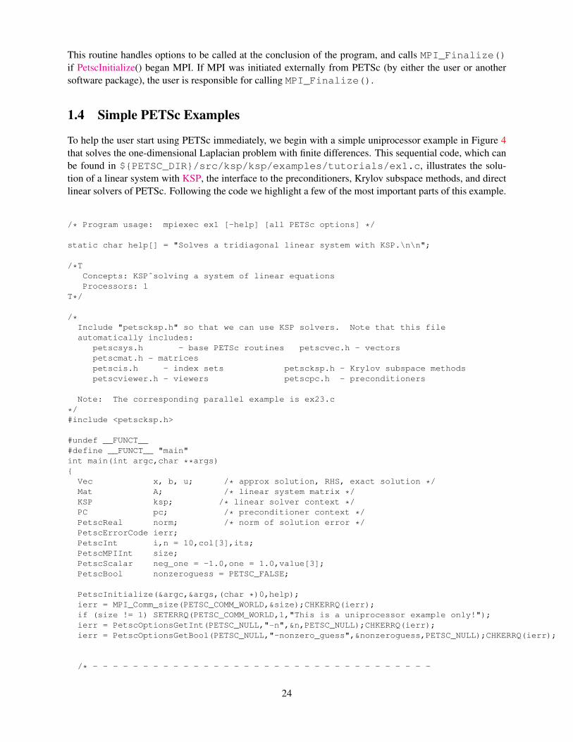
1.4 Simple PETSc Examples
To help the user start using PETSc immediately, we begin with a simple uniprocessor example in Figure 4that solves the one-dimensional Laplacian problem with finite differences. This sequential code, which canbe found in ${PETSC_DIR}/src/ksp/ksp/examples/tutorials/ex1.c, illustrates the solu-tion of a linear system with KSP, the interface to the preconditioners, Krylov subspace methods, and directlinear solvers of PETSc. Following the code we highlight a few of the most important parts of this example.
/* Program usage: mpiexec ex1 [-help] [all PETSc options] */
static char help[] = "Solves a tridiagonal linear system with KSP.\n\n";
/*TConcepts: KSPˆsolving a system of linear equationsProcessors: 1
T*/
/*Include "petscksp.h" so that we can use KSP solvers. Note that this fileautomatically includes:
petscsys.h - base PETSc routines petscvec.h - vectorspetscmat.h - matricespetscis.h - index sets petscksp.h - Krylov subspace methodspetscviewer.h - viewers petscpc.h - preconditioners
Note: The corresponding parallel example is ex23.c
*/#include <petscksp.h>
#undef __FUNCT__#define __FUNCT__ "main"int main(int argc,char **args){
Vec x, b, u; /* approx solution, RHS, exact solution */Mat A; /* linear system matrix */KSP ksp; /* linear solver context */PC pc; /* preconditioner context */PetscReal norm; /* norm of solution error */PetscErrorCode ierr;PetscInt i,n = 10,col[3],its;PetscMPIInt size;PetscScalar neg_one = -1.0,one = 1.0,value[3];PetscBool nonzeroguess = PETSC_FALSE;
PetscInitialize(&argc,&args,(char *)0,help);ierr = MPI_Comm_size(PETSC_COMM_WORLD,&size);CHKERRQ(ierr);if (size != 1) SETERRQ(PETSC_COMM_WORLD,1,"This is a uniprocessor example only!");ierr = PetscOptionsGetInt(PETSC_NULL,"-n",&n,PETSC_NULL);CHKERRQ(ierr);ierr = PetscOptionsGetBool(PETSC_NULL,"-nonzero_guess",&nonzeroguess,PETSC_NULL);CHKERRQ(ierr);
/* - - - - - - - - - - - - - - - - - - - - - - - - - - - - - - - - - -
24
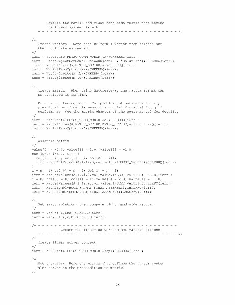
Compute the matrix and right-hand-side vector that definethe linear system, Ax = b.
- - - - - - - - - - - - - - - - - - - - - - - - - - - - - - - - - - */
/*Create vectors. Note that we form 1 vector from scratch andthen duplicate as needed.
*/ierr = VecCreate(PETSC_COMM_WORLD,&x);CHKERRQ(ierr);ierr = PetscObjectSetName((PetscObject) x, "Solution");CHKERRQ(ierr);ierr = VecSetSizes(x,PETSC_DECIDE,n);CHKERRQ(ierr);ierr = VecSetFromOptions(x);CHKERRQ(ierr);ierr = VecDuplicate(x,&b);CHKERRQ(ierr);ierr = VecDuplicate(x,&u);CHKERRQ(ierr);
/*Create matrix. When using MatCreate(), the matrix format canbe specified at runtime.
Performance tuning note: For problems of substantial size,preallocation of matrix memory is crucial for attaining goodperformance. See the matrix chapter of the users manual for details.
*/ierr = MatCreate(PETSC_COMM_WORLD,&A);CHKERRQ(ierr);ierr = MatSetSizes(A,PETSC_DECIDE,PETSC_DECIDE,n,n);CHKERRQ(ierr);ierr = MatSetFromOptions(A);CHKERRQ(ierr);
/*Assemble matrix
*/value[0] = -1.0; value[1] = 2.0; value[2] = -1.0;for (i=1; i<n-1; i++) {col[0] = i-1; col[1] = i; col[2] = i+1;ierr = MatSetValues(A,1,&i,3,col,value,INSERT_VALUES);CHKERRQ(ierr);
}i = n - 1; col[0] = n - 2; col[1] = n - 1;ierr = MatSetValues(A,1,&i,2,col,value,INSERT_VALUES);CHKERRQ(ierr);i = 0; col[0] = 0; col[1] = 1; value[0] = 2.0; value[1] = -1.0;ierr = MatSetValues(A,1,&i,2,col,value,INSERT_VALUES);CHKERRQ(ierr);ierr = MatAssemblyBegin(A,MAT_FINAL_ASSEMBLY);CHKERRQ(ierr);ierr = MatAssemblyEnd(A,MAT_FINAL_ASSEMBLY);CHKERRQ(ierr);
/*Set exact solution; then compute right-hand-side vector.
*/ierr = VecSet(u,one);CHKERRQ(ierr);ierr = MatMult(A,u,b);CHKERRQ(ierr);
/* - - - - - - - - - - - - - - - - - - - - - - - - - - - - - - - - - -Create the linear solver and set various options
- - - - - - - - - - - - - - - - - - - - - - - - - - - - - - - - - - *//*
Create linear solver context
*/ierr = KSPCreate(PETSC_COMM_WORLD,&ksp);CHKERRQ(ierr);
/*Set operators. Here the matrix that defines the linear systemalso serves as the preconditioning matrix.
*/
25
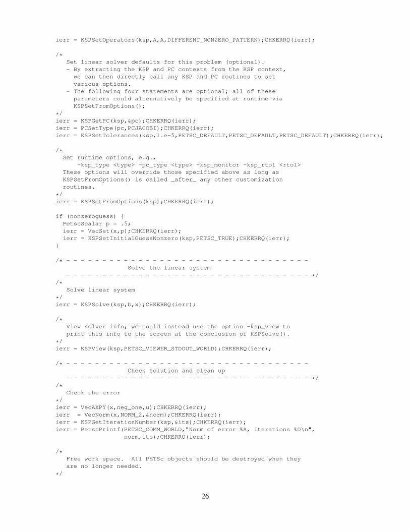
ierr = KSPSetOperators(ksp,A,A,DIFFERENT_NONZERO_PATTERN);CHKERRQ(ierr);
/*Set linear solver defaults for this problem (optional).- By extracting the KSP and PC contexts from the KSP context,
we can then directly call any KSP and PC routines to setvarious options.
- The following four statements are optional; all of theseparameters could alternatively be specified at runtime viaKSPSetFromOptions();
*/ierr = KSPGetPC(ksp,&pc);CHKERRQ(ierr);ierr = PCSetType(pc,PCJACOBI);CHKERRQ(ierr);ierr = KSPSetTolerances(ksp,1.e-5,PETSC_DEFAULT,PETSC_DEFAULT,PETSC_DEFAULT);CHKERRQ(ierr);
/*Set runtime options, e.g.,
-ksp_type <type> -pc_type <type> -ksp_monitor -ksp_rtol <rtol>These options will override those specified above as long asKSPSetFromOptions() is called _after_ any other customizationroutines.
*/ierr = KSPSetFromOptions(ksp);CHKERRQ(ierr);
if (nonzeroguess) {PetscScalar p = .5;ierr = VecSet(x,p);CHKERRQ(ierr);ierr = KSPSetInitialGuessNonzero(ksp,PETSC_TRUE);CHKERRQ(ierr);
}
/* - - - - - - - - - - - - - - - - - - - - - - - - - - - - - - - - - -Solve the linear system
- - - - - - - - - - - - - - - - - - - - - - - - - - - - - - - - - - *//*
Solve linear system
*/ierr = KSPSolve(ksp,b,x);CHKERRQ(ierr);
/*View solver info; we could instead use the option -ksp_view toprint this info to the screen at the conclusion of KSPSolve().
*/ierr = KSPView(ksp,PETSC_VIEWER_STDOUT_WORLD);CHKERRQ(ierr);
/* - - - - - - - - - - - - - - - - - - - - - - - - - - - - - - - - - -Check solution and clean up
- - - - - - - - - - - - - - - - - - - - - - - - - - - - - - - - - - *//*
Check the error
*/ierr = VecAXPY(x,neg_one,u);CHKERRQ(ierr);ierr = VecNorm(x,NORM_2,&norm);CHKERRQ(ierr);ierr = KSPGetIterationNumber(ksp,&its);CHKERRQ(ierr);ierr = PetscPrintf(PETSC_COMM_WORLD,"Norm of error %A, Iterations %D\n",
norm,its);CHKERRQ(ierr);
/*Free work space. All PETSc objects should be destroyed when theyare no longer needed.
*/
26
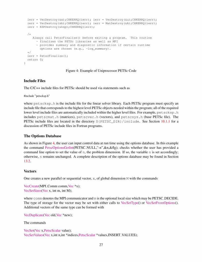
ierr = VecDestroy(&x);CHKERRQ(ierr); ierr = VecDestroy(&u);CHKERRQ(ierr);ierr = VecDestroy(&b);CHKERRQ(ierr); ierr = MatDestroy(&A);CHKERRQ(ierr);ierr = KSPDestroy(&ksp);CHKERRQ(ierr);
/*Always call PetscFinalize() before exiting a program. This routine
- finalizes the PETSc libraries as well as MPI- provides summary and diagnostic information if certain runtimeoptions are chosen (e.g., -log_summary).
*/ierr = PetscFinalize();return 0;
}
Figure 4: Example of Uniprocessor PETSc Code
Include Files
The C/C++ include files for PETSc should be used via statements such as
#include ”petscksp.h”
where petscksp.h is the include file for the linear solver library. Each PETSc program must specify aninclude file that corresponds to the highest level PETSc objects needed within the program; all of the requiredlower level include files are automatically included within the higher level files. For example, petscksp.hincludes petscmat.h (matrices), petscvec.h (vectors), and petscsys.h (base PETSc file). ThePETSc include files are located in the directory ${PETSC_DIR}/include. See Section 10.1.1 for adiscussion of PETSc include files in Fortran programs.
The Options Database
As shown in Figure 4, the user can input control data at run time using the options database. In this examplethe command PetscOptionsGetInt(PETSC NULL,”-n”,&n,&flg); checks whether the user has provided acommand line option to set the value of n, the problem dimension. If so, the variable n is set accordingly;otherwise, n remains unchanged. A complete description of the options database may be found in Section13.2.
Vectors
One creates a new parallel or sequential vector, x, of global dimension M with the commands
VecCreate(MPI Comm comm,Vec *x);VecSetSizes(Vec x, int m, int M);
where comm denotes the MPI communicator and m is the optional local size which may be PETSC DECIDE.The type of storage for the vector may be set with either calls to VecSetType() or VecSetFromOptions().Additional vectors of the same type can be formed with
VecDuplicate(Vec old,Vec *new);
The commands
VecSet(Vec x,PetscScalar value);VecSetValues(Vec x,int n,int *indices,PetscScalar *values,INSERT VALUES);
27
respectively set all the components of a vector to a particular scalar value and assign a different value toeach component. More detailed information about PETSc vectors, including their basic operations, scatter-ing/gathering, index sets, and distributed arrays, is discussed in Chapter 2.
Note the use of the PETSc variable type PetscScalar in this example. The PetscScalar is simply definedto be double in C/C++ (or correspondingly double precision in Fortran) for versions of PETSc thathave not been compiled for use with complex numbers. The PetscScalar data type enables identical code tobe used when the PETSc libraries have been compiled for use with complex numbers. Section 13.7 discussesthe use of complex numbers in PETSc programs.
Matrices
Usage of PETSc matrices and vectors is similar. The user can create a new parallel or sequential matrix, A,which has M global rows and N global columns, with the routines
MatCreate(MPI Comm comm,Mat *A);MatSetSizes(Mat A,int m,int n,int M,int N);
where the matrix format can be specified at runtime. The user could alternatively specify each processes’number of local rows and columns using m and n. Generally one then sets the ”type” of the matrix, with, forexample,
MatSetType(Mat A,MATAIJ);
This causes the matrix to used the compressed sparse row storage format to store the matrix entries. SeeMatType for a list of all matrix types. Values can then be set with the command
MatSetValues(Mat A,int m,int *im,int n,int *in,PetscScalar *values,INSERT VALUES);
After all elements have been inserted into the matrix, it must be processed with the pair of commands
MatAssemblyBegin(Mat A,MAT FINAL ASSEMBLY);MatAssemblyEnd(Mat A,MAT FINAL ASSEMBLY);
Chapter 3 discusses various matrix formats as well as the details of some basic matrix manipulation routines.
Linear Solvers
After creating the matrix and vectors that define a linear system, Ax = b, the user can then use KSP tosolve the system with the following sequence of commands:
KSPCreate(MPI Comm comm,KSP *ksp);KSPSetOperators(KSP ksp,Mat A,Mat PrecA,MatStructure flag);KSPSetFromOptions(KSP ksp);KSPSolve(KSP ksp,Vec b,Vec x);KSPDestroy(KSP ksp);
The user first creates the KSP context and sets the operators associated with the system (linear system matrixand optionally different preconditioning matrix). The user then sets various options for customized solution,solves the linear system, and finally destroys the KSP context. We emphasize the command KSPSetFro-mOptions(), which enables the user to customize the linear solution method at runtime by using the optionsdatabase, which is discussed in Section 13.2. Through this database, the user not only can select an iter-ative method and preconditioner, but also can prescribe the convergence tolerance, set various monitoringroutines, etc. (see, e.g., Figure 8).
Chapter 4 describes in detail the KSP package, including the PC and KSP packages for preconditionersand Krylov subspace methods.
28
Nonlinear Solvers
Most PDE problems of interest are inherently nonlinear. PETSc provides an interface to tackle the nonlinearproblems directly called SNES. Chapter 5 describes the nonlinear solvers in detail. We recommend mostPETSc users work directly with SNES, rather than using PETSc for the linear problem within a nonlinearsolver.
Error Checking
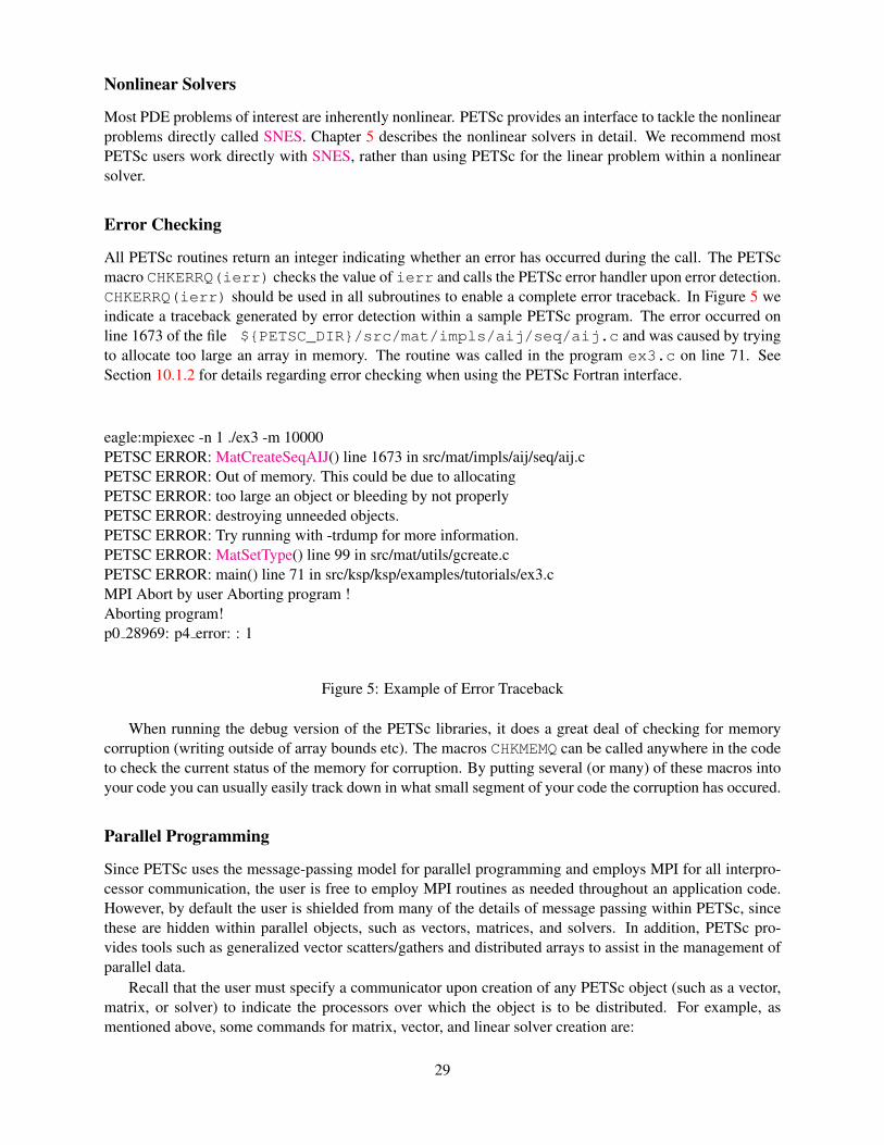
All PETSc routines return an integer indicating whether an error has occurred during the call. The PETScmacro CHKERRQ(ierr) checks the value of ierr and calls the PETSc error handler upon error detection.CHKERRQ(ierr) should be used in all subroutines to enable a complete error traceback. In Figure 5 weindicate a traceback generated by error detection within a sample PETSc program. The error occurred online 1673 of the file ${PETSC_DIR}/src/mat/impls/aij/seq/aij.c and was caused by tryingto allocate too large an array in memory. The routine was called in the program ex3.c on line 71. SeeSection 10.1.2 for details regarding error checking when using the PETSc Fortran interface.
eagle:mpiexec -n 1 ./ex3 -m 10000PETSC ERROR: MatCreateSeqAIJ() line 1673 in src/mat/impls/aij/seq/aij.cPETSC ERROR: Out of memory. This could be due to allocatingPETSC ERROR: too large an object or bleeding by not properlyPETSC ERROR: destroying unneeded objects.PETSC ERROR: Try running with -trdump for more information.PETSC ERROR: MatSetType() line 99 in src/mat/utils/gcreate.cPETSC ERROR: main() line 71 in src/ksp/ksp/examples/tutorials/ex3.cMPI Abort by user Aborting program !Aborting program!p0 28969: p4 error: : 1
Figure 5: Example of Error Traceback
When running the debug version of the PETSc libraries, it does a great deal of checking for memorycorruption (writing outside of array bounds etc). The macros CHKMEMQ can be called anywhere in the codeto check the current status of the memory for corruption. By putting several (or many) of these macros intoyour code you can usually easily track down in what small segment of your code the corruption has occured.
Parallel Programming
Since PETSc uses the message-passing model for parallel programming and employs MPI for all interpro-cessor communication, the user is free to employ MPI routines as needed throughout an application code.However, by default the user is shielded from many of the details of message passing within PETSc, sincethese are hidden within parallel objects, such as vectors, matrices, and solvers. In addition, PETSc pro-vides tools such as generalized vector scatters/gathers and distributed arrays to assist in the management ofparallel data.
Recall that the user must specify a communicator upon creation of any PETSc object (such as a vector,matrix, or solver) to indicate the processors over which the object is to be distributed. For example, asmentioned above, some commands for matrix, vector, and linear solver creation are:
29
MatCreate(MPI Comm comm,Mat *A);VecCreate(MPI Comm comm,Vec *x);KSPCreate(MPI Comm comm,KSP *ksp);
The creation routines are collective over all processors in the communicator; thus, all processors in thecommunicator must call the creation routine. In addition, if a sequence of collective routines is being used,they must be called in the same order on each processor.
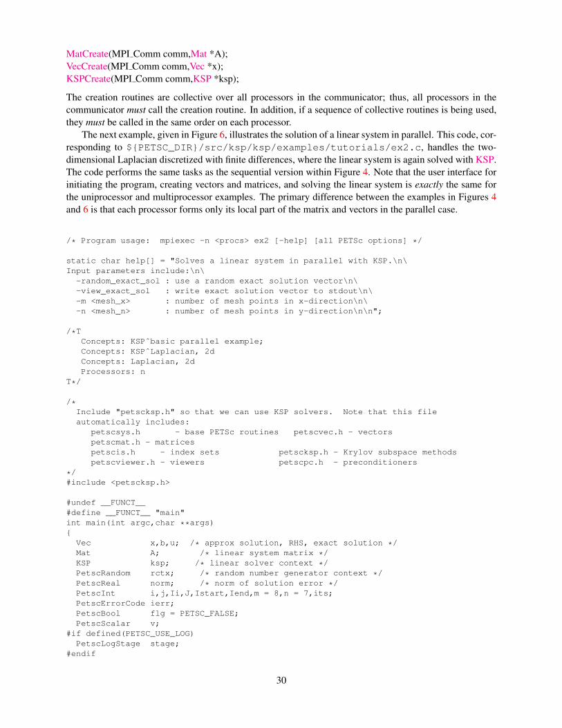
The next example, given in Figure 6, illustrates the solution of a linear system in parallel. This code, cor-responding to ${PETSC_DIR}/src/ksp/ksp/examples/tutorials/ex2.c, handles the two-dimensional Laplacian discretized with finite differences, where the linear system is again solved with KSP.The code performs the same tasks as the sequential version within Figure 4. Note that the user interface forinitiating the program, creating vectors and matrices, and solving the linear system is exactly the same forthe uniprocessor and multiprocessor examples. The primary difference between the examples in Figures 4and 6 is that each processor forms only its local part of the matrix and vectors in the parallel case.
/* Program usage: mpiexec -n <procs> ex2 [-help] [all PETSc options] */
static char help[] = "Solves a linear system in parallel with KSP.\n\Input parameters include:\n\
-random_exact_sol : use a random exact solution vector\n\-view_exact_sol : write exact solution vector to stdout\n\-m <mesh_x> : number of mesh points in x-direction\n\-n <mesh_n> : number of mesh points in y-direction\n\n";
/*TConcepts: KSPˆbasic parallel example;Concepts: KSPˆLaplacian, 2dConcepts: Laplacian, 2dProcessors: n
T*/
/*Include "petscksp.h" so that we can use KSP solvers. Note that this fileautomatically includes:
petscsys.h - base PETSc routines petscvec.h - vectorspetscmat.h - matricespetscis.h - index sets petscksp.h - Krylov subspace methodspetscviewer.h - viewers petscpc.h - preconditioners
*/#include <petscksp.h>
#undef __FUNCT__#define __FUNCT__ "main"int main(int argc,char **args){
Vec x,b,u; /* approx solution, RHS, exact solution */Mat A; /* linear system matrix */KSP ksp; /* linear solver context */PetscRandom rctx; /* random number generator context */PetscReal norm; /* norm of solution error */PetscInt i,j,Ii,J,Istart,Iend,m = 8,n = 7,its;PetscErrorCode ierr;PetscBool flg = PETSC_FALSE;PetscScalar v;
#if defined(PETSC_USE_LOG)PetscLogStage stage;
#endif
30
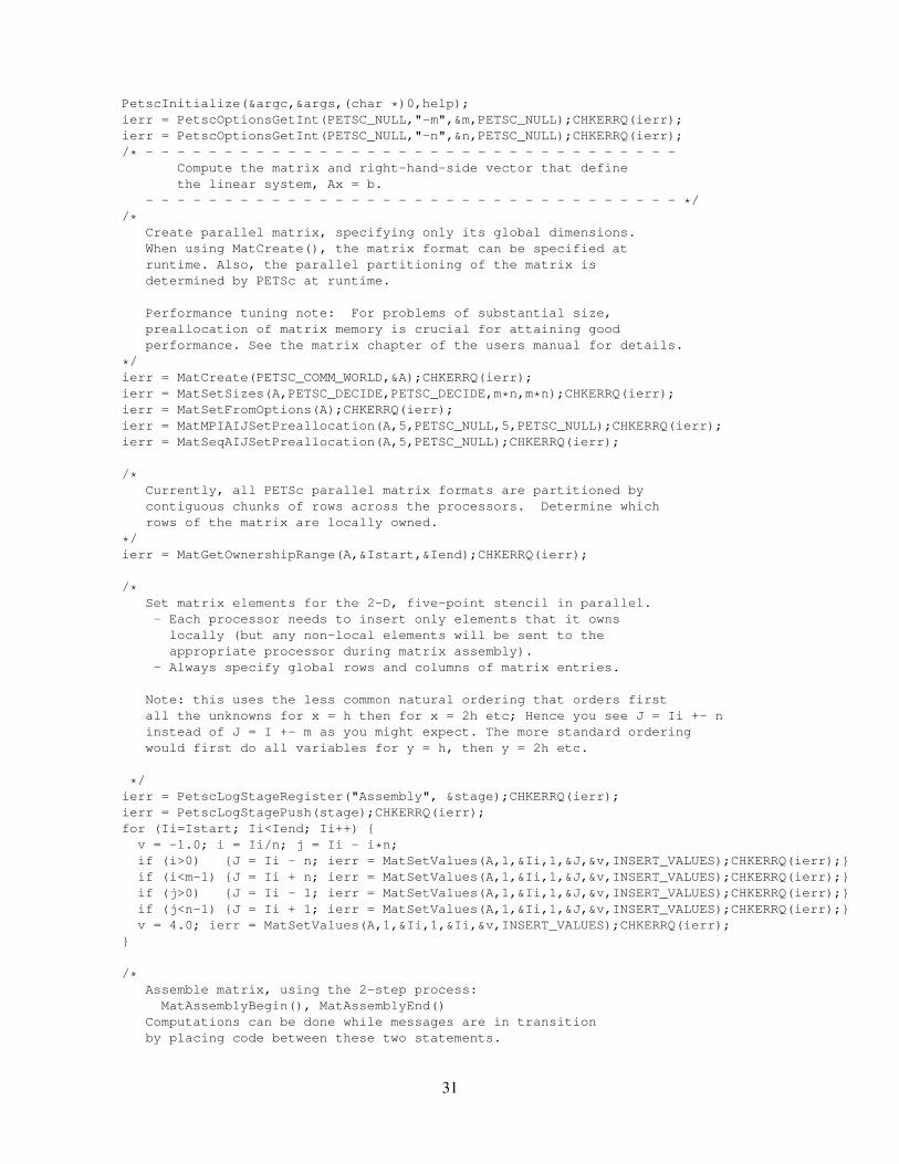
PetscInitialize(&argc,&args,(char *)0,help);ierr = PetscOptionsGetInt(PETSC_NULL,"-m",&m,PETSC_NULL);CHKERRQ(ierr);ierr = PetscOptionsGetInt(PETSC_NULL,"-n",&n,PETSC_NULL);CHKERRQ(ierr);/* - - - - - - - - - - - - - - - - - - - - - - - - - - - - - - - - - -
Compute the matrix and right-hand-side vector that definethe linear system, Ax = b.
- - - - - - - - - - - - - - - - - - - - - - - - - - - - - - - - - - *//*
Create parallel matrix, specifying only its global dimensions.When using MatCreate(), the matrix format can be specified atruntime. Also, the parallel partitioning of the matrix isdetermined by PETSc at runtime.
Performance tuning note: For problems of substantial size,preallocation of matrix memory is crucial for attaining goodperformance. See the matrix chapter of the users manual for details.
*/ierr = MatCreate(PETSC_COMM_WORLD,&A);CHKERRQ(ierr);ierr = MatSetSizes(A,PETSC_DECIDE,PETSC_DECIDE,m*n,m*n);CHKERRQ(ierr);ierr = MatSetFromOptions(A);CHKERRQ(ierr);ierr = MatMPIAIJSetPreallocation(A,5,PETSC_NULL,5,PETSC_NULL);CHKERRQ(ierr);ierr = MatSeqAIJSetPreallocation(A,5,PETSC_NULL);CHKERRQ(ierr);
/*Currently, all PETSc parallel matrix formats are partitioned bycontiguous chunks of rows across the processors. Determine whichrows of the matrix are locally owned.
*/ierr = MatGetOwnershipRange(A,&Istart,&Iend);CHKERRQ(ierr);
/*Set matrix elements for the 2-D, five-point stencil in parallel.- Each processor needs to insert only elements that it owns
locally (but any non-local elements will be sent to theappropriate processor during matrix assembly).
- Always specify global rows and columns of matrix entries.
Note: this uses the less common natural ordering that orders firstall the unknowns for x = h then for x = 2h etc; Hence you see J = Ii +- ninstead of J = I +- m as you might expect. The more standard orderingwould first do all variables for y = h, then y = 2h etc.
*/ierr = PetscLogStageRegister("Assembly", &stage);CHKERRQ(ierr);ierr = PetscLogStagePush(stage);CHKERRQ(ierr);for (Ii=Istart; Ii<Iend; Ii++) {v = -1.0; i = Ii/n; j = Ii - i*n;if (i>0) {J = Ii - n; ierr = MatSetValues(A,1,&Ii,1,&J,&v,INSERT_VALUES);CHKERRQ(ierr);}if (i<m-1) {J = Ii + n; ierr = MatSetValues(A,1,&Ii,1,&J,&v,INSERT_VALUES);CHKERRQ(ierr);}if (j>0) {J = Ii - 1; ierr = MatSetValues(A,1,&Ii,1,&J,&v,INSERT_VALUES);CHKERRQ(ierr);}if (j<n-1) {J = Ii + 1; ierr = MatSetValues(A,1,&Ii,1,&J,&v,INSERT_VALUES);CHKERRQ(ierr);}v = 4.0; ierr = MatSetValues(A,1,&Ii,1,&Ii,&v,INSERT_VALUES);CHKERRQ(ierr);
}
/*Assemble matrix, using the 2-step process:
MatAssemblyBegin(), MatAssemblyEnd()Computations can be done while messages are in transitionby placing code between these two statements.
31
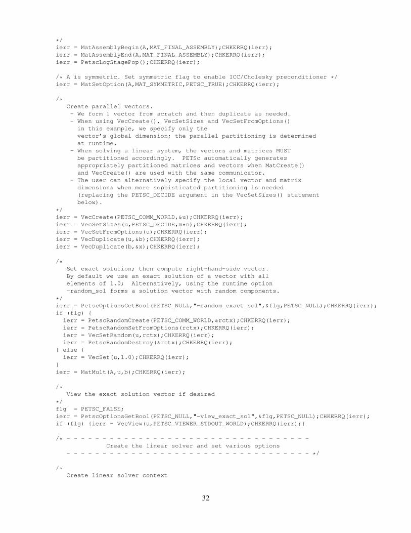
*/ierr = MatAssemblyBegin(A,MAT_FINAL_ASSEMBLY);CHKERRQ(ierr);ierr = MatAssemblyEnd(A,MAT_FINAL_ASSEMBLY);CHKERRQ(ierr);ierr = PetscLogStagePop();CHKERRQ(ierr);
/* A is symmetric. Set symmetric flag to enable ICC/Cholesky preconditioner */ierr = MatSetOption(A,MAT_SYMMETRIC,PETSC_TRUE);CHKERRQ(ierr);
/*Create parallel vectors.- We form 1 vector from scratch and then duplicate as needed.- When using VecCreate(), VecSetSizes and VecSetFromOptions()
in this example, we specify only thevector’s global dimension; the parallel partitioning is determinedat runtime.
- When solving a linear system, the vectors and matrices MUSTbe partitioned accordingly. PETSc automatically generatesappropriately partitioned matrices and vectors when MatCreate()and VecCreate() are used with the same communicator.
- The user can alternatively specify the local vector and matrixdimensions when more sophisticated partitioning is needed(replacing the PETSC_DECIDE argument in the VecSetSizes() statementbelow).
*/ierr = VecCreate(PETSC_COMM_WORLD,&u);CHKERRQ(ierr);ierr = VecSetSizes(u,PETSC_DECIDE,m*n);CHKERRQ(ierr);ierr = VecSetFromOptions(u);CHKERRQ(ierr);ierr = VecDuplicate(u,&b);CHKERRQ(ierr);ierr = VecDuplicate(b,&x);CHKERRQ(ierr);
/*Set exact solution; then compute right-hand-side vector.By default we use an exact solution of a vector with allelements of 1.0; Alternatively, using the runtime option-random_sol forms a solution vector with random components.
*/ierr = PetscOptionsGetBool(PETSC_NULL,"-random_exact_sol",&flg,PETSC_NULL);CHKERRQ(ierr);if (flg) {ierr = PetscRandomCreate(PETSC_COMM_WORLD,&rctx);CHKERRQ(ierr);ierr = PetscRandomSetFromOptions(rctx);CHKERRQ(ierr);ierr = VecSetRandom(u,rctx);CHKERRQ(ierr);ierr = PetscRandomDestroy(&rctx);CHKERRQ(ierr);
} else {ierr = VecSet(u,1.0);CHKERRQ(ierr);
}ierr = MatMult(A,u,b);CHKERRQ(ierr);
/*View the exact solution vector if desired
*/flg = PETSC_FALSE;ierr = PetscOptionsGetBool(PETSC_NULL,"-view_exact_sol",&flg,PETSC_NULL);CHKERRQ(ierr);if (flg) {ierr = VecView(u,PETSC_VIEWER_STDOUT_WORLD);CHKERRQ(ierr);}
/* - - - - - - - - - - - - - - - - - - - - - - - - - - - - - - - - - -Create the linear solver and set various options
- - - - - - - - - - - - - - - - - - - - - - - - - - - - - - - - - - */
/*Create linear solver context
32
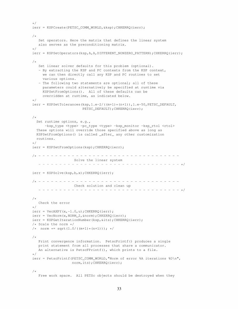
*/ierr = KSPCreate(PETSC_COMM_WORLD,&ksp);CHKERRQ(ierr);
/*Set operators. Here the matrix that defines the linear systemalso serves as the preconditioning matrix.
*/ierr = KSPSetOperators(ksp,A,A,DIFFERENT_NONZERO_PATTERN);CHKERRQ(ierr);
/*Set linear solver defaults for this problem (optional).- By extracting the KSP and PC contexts from the KSP context,
we can then directly call any KSP and PC routines to setvarious options.
- The following two statements are optional; all of theseparameters could alternatively be specified at runtime viaKSPSetFromOptions(). All of these defaults can beoverridden at runtime, as indicated below.
*/ierr = KSPSetTolerances(ksp,1.e-2/((m+1)*(n+1)),1.e-50,PETSC_DEFAULT,
PETSC_DEFAULT);CHKERRQ(ierr);
/*Set runtime options, e.g.,
-ksp_type <type> -pc_type <type> -ksp_monitor -ksp_rtol <rtol>These options will override those specified above as long asKSPSetFromOptions() is called _after_ any other customizationroutines.
*/ierr = KSPSetFromOptions(ksp);CHKERRQ(ierr);
/* - - - - - - - - - - - - - - - - - - - - - - - - - - - - - - - - - -Solve the linear system
- - - - - - - - - - - - - - - - - - - - - - - - - - - - - - - - - - */
ierr = KSPSolve(ksp,b,x);CHKERRQ(ierr);
/* - - - - - - - - - - - - - - - - - - - - - - - - - - - - - - - - - -Check solution and clean up
- - - - - - - - - - - - - - - - - - - - - - - - - - - - - - - - - - */
/*Check the error
*/ierr = VecAXPY(x,-1.0,u);CHKERRQ(ierr);ierr = VecNorm(x,NORM_2,&norm);CHKERRQ(ierr);ierr = KSPGetIterationNumber(ksp,&its);CHKERRQ(ierr);/* Scale the norm *//* norm *= sqrt(1.0/((m+1)*(n+1))); */
/*Print convergence information. PetscPrintf() produces a singleprint statement from all processes that share a communicator.An alternative is PetscFPrintf(), which prints to a file.
*/ierr = PetscPrintf(PETSC_COMM_WORLD,"Norm of error %A iterations %D\n",
norm,its);CHKERRQ(ierr);
/*Free work space. All PETSc objects should be destroyed when they
33
are no longer needed.
*/ierr = KSPDestroy(&ksp);CHKERRQ(ierr);ierr = VecDestroy(&u);CHKERRQ(ierr); ierr = VecDestroy(&x);CHKERRQ(ierr);ierr = VecDestroy(&b);CHKERRQ(ierr); ierr = MatDestroy(&A);CHKERRQ(ierr);
/*Always call PetscFinalize() before exiting a program. This routine
- finalizes the PETSc libraries as well as MPI- provides summary and diagnostic information if certain runtimeoptions are chosen (e.g., -log_summary).
*/ierr = PetscFinalize();return 0;
}
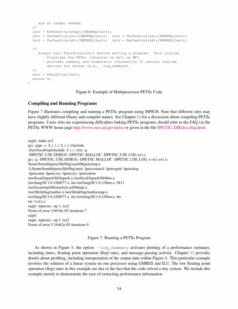
Figure 6: Example of Multiprocessor PETSc Code
Compiling and Running Programs
Figure 7 illustrates compiling and running a PETSc program using MPICH. Note that different sites mayhave slightly different library and compiler names. See Chapter 14 for a discussion about compiling PETScprograms. Users who are experiencing difficulties linking PETSc programs should refer to the FAQ via thePETSc WWW home page http://www.mcs.anl.gov/petsc or given in the file $PETSC DIR/docs/faq.html.
eagle: make ex2gcc -pipe -c -I../../../ -I../../..//include-I/usr/local/mpi/include -I../../..//src -g-DPETSC USE DEBUG -DPETSC MALLOC -DPETSC USE LOG ex1.cgcc -g -DPETSC USE DEBUG -DPETSC MALLOC -DPETSC USE LOG -o ex1 ex1.o/home/bsmith/petsc/lib/libg/sun4/libpetscksp.a-L/home/bsmith/petsc/lib/libg/sun4 -lpetscstencil -lpetscgrid -lpetscksp-lpetscmat -lpetscvec -lpetscsys -lpetscdraw/usr/local/lapack/lib/lapack.a /usr/local/lapack/lib/blas.a/usr/lang/SC1.0.1/libF77.a -lm /usr/lang/SC1.0.1/libm.a -lX11/usr/local/mpi/lib/sun4/ch p4/libmpi.a/usr/lib/debug/malloc.o /usr/lib/debug/mallocmap.o/usr/lang/SC1.0.1/libF77.a -lm /usr/lang/SC1.0.1/libm.a -lmrm -f ex1.oeagle: mpiexec -np 1 ./ex2Norm of error 3.6618e-05 iterations 7eagle:eagle: mpiexec -np 2 ./ex2Norm of error 5.34462e-05 iterations 9
Figure 7: Running a PETSc Program
As shown in Figure 8, the option -log_summary activates printing of a performance summary,including times, floating point operation (flop) rates, and message-passing activity. Chapter 11 providesdetails about profiling, including interpretation of the output data within Figure 8. This particular exampleinvolves the solution of a linear system on one processor using GMRES and ILU. The low floating pointoperation (flop) rates in this example are due to the fact that the code solved a tiny system. We include thisexample merely to demonstrate the ease of extracting performance information.
34
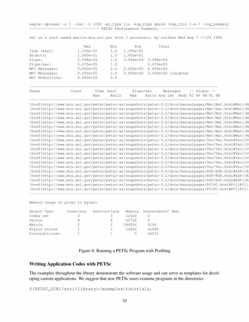
eagle> mpiexec -n 1 ./ex1 -n 1000 -pc_type ilu -ksp_type gmres -ksp_rtol 1.e-7 -log_summary-------------------------------- PETSc Performance Summary: -------------------------------
ex1 on a sun4 named merlin.mcs.anl.gov with 1 processor, by curfman Wed Aug 7 17:24 1996
Max Min Avg TotalTime (sec): 1.150e-01 1.0 1.150e-01Objects: 1.900e+01 1.0 1.900e+01Flops: 3.998e+04 1.0 3.998e+04 3.998e+04Flops/sec: 3.475e+05 1.0 3.475e+05MPI Messages: 0.000e+00 0.0 0.000e+00 0.000e+00MPI Messages: 0.000e+00 0.0 0.000e+00 0.000e+00 (lengths)MPI Reductions: 0.000e+00 0.0
--------------------------------------------------------------------------------------Phase Count Time (sec) Flops/sec Messages -- Global --
Max Ratio Max Ratio Avg len Redc %T %F %M %L %R--------------------------------------------------------------------------------------\href{http://www.mcs.anl.gov/petsc/petsc-as/snapshots/petsc-3.2/docs/manualpages/Mat/Mat.html#Mat}{Mat}\findex{Mat} Mult 2 2.553e-03 1.0 3.9e+06 1.0 0.0 0.0 0.0 2 25 0 0 0\href{http://www.mcs.anl.gov/petsc/petsc-as/snapshots/petsc-3.2/docs/manualpages/Mat/Mat.html#Mat}{Mat}\findex{Mat} AssemblyBegin 1 2.193e-05 1.0 0.0e+00 0.0 0.0 0.0 0.0 0 0 0 0 0\href{http://www.mcs.anl.gov/petsc/petsc-as/snapshots/petsc-3.2/docs/manualpages/Mat/Mat.html#Mat}{Mat}\findex{Mat} AssemblyEnd 1 5.004e-03 1.0 0.0e+00 0.0 0.0 0.0 0.0 4 0 0 0 0\href{http://www.mcs.anl.gov/petsc/petsc-as/snapshots/petsc-3.2/docs/manualpages/Mat/Mat.html#Mat}{Mat}\findex{Mat} GetOrdering 1 3.004e-03 1.0 0.0e+00 0.0 0.0 0.0 0.0 3 0 0 0 0\href{http://www.mcs.anl.gov/petsc/petsc-as/snapshots/petsc-3.2/docs/manualpages/Mat/Mat.html#Mat}{Mat}\findex{Mat} ILUFctrSymbol 1 5.719e-03 1.0 0.0e+00 0.0 0.0 0.0 0.0 5 0 0 0 0\href{http://www.mcs.anl.gov/petsc/petsc-as/snapshots/petsc-3.2/docs/manualpages/Mat/Mat.html#Mat}{Mat}\findex{Mat} LUFactorNumer 1 1.092e-02 1.0 2.7e+05 1.0 0.0 0.0 0.0 9 7 0 0 0\href{http://www.mcs.anl.gov/petsc/petsc-as/snapshots/petsc-3.2/docs/manualpages/Mat/Mat.html#Mat}{Mat}\findex{Mat} Solve 2 4.193e-03 1.0 2.4e+06 1.0 0.0 0.0 0.0 4 25 0 0 0\href{http://www.mcs.anl.gov/petsc/petsc-as/snapshots/petsc-3.2/docs/manualpages/Mat/Mat.html#Mat}{Mat}\findex{Mat} SetValues 1000 2.461e-02 1.0 0.0e+00 0.0 0.0 0.0 0.0 21 0 0 0 0\href{http://www.mcs.anl.gov/petsc/petsc-as/snapshots/petsc-3.2/docs/manualpages/Vec/Vec.html#Vec}{Vec}\findex{Vec} Dot 1 60e-04 1.0 9.7e+06 1.0 0.0 0.0 0.0 0 5 0 0 0\href{http://www.mcs.anl.gov/petsc/petsc-as/snapshots/petsc-3.2/docs/manualpages/Vec/Vec.html#Vec}{Vec}\findex{Vec} Norm 3 5.870e-04 1.0 1.0e+07 1.0 0.0 0.0 0.0 1 15 0 0 0\href{http://www.mcs.anl.gov/petsc/petsc-as/snapshots/petsc-3.2/docs/manualpages/Vec/Vec.html#Vec}{Vec}\findex{Vec} Scale 1 1.640e-04 1.0 6.1e+06 1.0 0.0 0.0 0.0 0 3 0 0 0\href{http://www.mcs.anl.gov/petsc/petsc-as/snapshots/petsc-3.2/docs/manualpages/Vec/Vec.html#Vec}{Vec}\findex{Vec} Copy 1 3.101e-04 1.0 0.0e+00 0.0 0.0 0.0 0.0 0 0 0 0 0\href{http://www.mcs.anl.gov/petsc/petsc-as/snapshots/petsc-3.2/docs/manualpages/Vec/Vec.html#Vec}{Vec}\findex{Vec} Set 3 5.029e-04 1.0 0.0e+00 0.0 0.0 0.0 0.0 0 0 0 0 0\href{http://www.mcs.anl.gov/petsc/petsc-as/snapshots/petsc-3.2/docs/manualpages/Vec/Vec.html#Vec}{Vec}\findex{Vec} AXPY 3 8.690e-04 1.0 6.9e+06 1.0 0.0 0.0 0.0 1 15 0 0 0\href{http://www.mcs.anl.gov/petsc/petsc-as/snapshots/petsc-3.2/docs/manualpages/Vec/Vec.html#Vec}{Vec}\findex{Vec} MAXPY 1 2.550e-04 1.0 7.8e+06 1.0 0.0 0.0 0.0 0 5 0 0 0\href{http://www.mcs.anl.gov/petsc/petsc-as/snapshots/petsc-3.2/docs/manualpages/KSP/KSP.html#KSP}{KSP}\findex{KSP} Solve 1 1.288e-02 1.0 2.2e+06 1.0 0.0 0.0 0.0 11 70 0 0 0\href{http://www.mcs.anl.gov/petsc/petsc-as/snapshots/petsc-3.2/docs/manualpages/KSP/KSP.html#KSP}{KSP}\findex{KSP} SetUp 1 2.669e-02 1.0 1.1e+05 1.0 0.0 0.0 0.0 23 7 0 0 0\href{http://www.mcs.anl.gov/petsc/petsc-as/snapshots/petsc-3.2/docs/manualpages/KSP/KSP.html#KSP}{KSP}\findex{KSP} GMRESOrthog 1 1.151e-03 1.0 3.5e+06 1.0 0.0 0.0 0.0 1 10 0 0 0\href{http://www.mcs.anl.gov/petsc/petsc-as/snapshots/petsc-3.2/docs/manualpages/PC/PC.html#PC}{PC}\findex{PC} SetUp 1 2.4e-02 1.0 1.5e+05 1.0 0.0 0.0 0.0 18 7 0 0 0\href{http://www.mcs.anl.gov/petsc/petsc-as/snapshots/petsc-3.2/docs/manualpages/PC/PC.html#PC}{PC}\findex{PC} Apply 2 4.474e-03 1.0 2.2e+06 1.0 0.0 0.0 0.0 4 25 0 0 0--------------------------------------------------------------------------------------
Memory usage is given in bytes:
Object Type Creations Destructions Memory Descendants’ Mem.Index set 3 3 12420 0Vector 8 8 65728 0Matrix 2 2 184924 4140Krylov Solver 1 1 16892 41080Preconditioner 1 1 0 64872
Figure 8: Running a PETSc Program with Profiling
Writing Application Codes with PETSc
The examples throughout the library demonstrate the software usage and can serve as templates for devel-oping custom applications. We suggest that new PETSc users examine programs in the directories
${PETSC_DIR}/src/<library>/examples/tutorials,
35
where <library> denotes any of the PETSc libraries (listed in the following section), such as snes orksp. The manual pages located at
$PETSC DIR/docs/index.html orhttp://www.mcs.anl.gov/petsc/petsc-as/documentation
provide indices (organized by both routine names and concepts) to the tutorial examples.To write a new application program using PETSc, we suggest the following procedure:
1. Install and test PETSc according to the instructions at the PETSc web site.
2. Copy one of the many PETSc examples in the directory that corresponds to the class of problem ofinterest (e.g., for linear solvers, see ${PETSC_DIR}/src/ksp/ksp/examples/tutorials).
3. Copy the corresponding makefile within the example directory; compile and run the example program.
4. Use the example program as a starting point for developing a custom code.
1.5 Referencing PETSc
When referencing PETSc in a publication please cite the following:
@Unpublished{petsc-home-page,Author = ”Satish Balay and William D. Gropp and Lois C. McInnes and Barry F. Smith”,Title = ”PETSc home page”,Note = ”http://www.mcs.anl.gov/petsc”,Year = ”2008”}
@TechReport{petsc-manual,Author = ”Satish Balay and William D. Gropp and Lois C. McInnes and Barry F. Smith”,Title = ”PETSc Users Manual”,Number = ”ANL-95/11 - Revision 3.2”,Institution = ”Argonne National Laboratory”,Year = ”2011”}
@InProceedings{petsc-efficient,Author = ”Satish Balay and William D. Gropp and Lois C. McInnes and Barry F. Smith”,Title = ”Efficienct Management of Parallelism in Object Oriented Numerical Software Libraries”,Booktitle = ”Modern Software Tools in Scientific Computing”,Editor = ”E. Arge and A. M. Bruaset and H. P. Langtangen”,Pages = ”163–202”,Publisher = ”Birkhauser Press”,Year = ”1997”}
1.6 Directory Structure
We conclude this introduction with an overview of the organization of the PETSc software. The root direc-tory of PETSc contains the following directories:
• docs - All documentation for PETSc. The files manual.pdf contains the hyperlinked users man-ual, suitable for printing or on-screen viewering. Includes the subdirectory
- manualpages (on-line manual pages).
36
• bin - Utilities and short scripts for use with PETSc, including
– petscmpiexec (utility for setting running MPI jobs),
• conf - Base PETSc makefile that defines the standard make variables and rules used by PETSc
• include - All include files for PETSc that are visible to the user.
• include/finclude - PETSc include files for Fortran programmers using the .F suffix (recom-mended).
• include/private - Private PETSc include files that should not be used by application program-mers.
• share - Some small test matrices in data files
• src - The source code for all PETSc libraries, which currently includes
– vec - vectors,
∗ is - index sets,
– mat - matrices,
– dm - data management between meshes and vectors and matrices,
– ksp - complete linear equations solvers,
∗ ksp - Krylov subspace accelerators,∗ pc - preconditioners,
– snes - nonlinear solvers
– ts - ODE solvers and timestepping,
– sys - general system-related routines,
∗ plog - PETSc logging and profiling routines,∗ draw - simple graphics,
– contrib - contributed modules that use PETSc but are not part of the official PETSc package.We encourage users who have developed such code that they wish to share with others to let usknow by writing to [email protected].
Each PETSc source code library directory has the following subdirectories:
• examples - Example programs for the component, including
– tutorials - Programs designed to teach users about PETSc. These codes can serve as tem-plates for the design of custom applications.
– tests - Programs designed for thorough testing of PETSc. As such, these codes are not in-tended for examination by users.
• interface - The calling sequences for the abstract interface to the component. Code here does notknow about particular implementations.
• impls - Source code for one or more implementations.
• utils - Utility routines. Source here may know about the implementations, but ideally will not knowabout implementations for other components.
37

38
Part II
Programming with PETSc
39

Chapter 2
Vectors and Distributing Parallel Data
The vector (denoted by Vec) is one of the simplest PETSc objects. Vectors are used to store discrete PDEsolutions, right-hand sides for linear systems, etc. This chapter is organized as follows:
• (Vec) Sections 2.1 and 2.2 - basic usage of vectors
• Section 2.3 - management of the various numberings of degrees of freedom, vertices, cells, etc.
– (AO) Mapping between different global numberings
– (ISLocalToGlobalMapping) Mapping between local and global numberings
• (DM) Section 2.4 - management of grids
• (IS, VecScatter) Section 2.5 - management of vectors related to unstructured grids
2.1 Creating and Assembling Vectors
PETSc currently provides two basic vector types: sequential and parallel (MPI based). To create a sequentialvector with m components, one can use the command
VecCreateSeq(PETSC COMM SELF,int m,Vec *x);
To create a parallel vector one can either specify the number of components that will be stored on eachprocess or let PETSc decide. The command
VecCreateMPI(MPI Comm comm,int m,int M,Vec *x);
creates a vector that is distributed over all processes in the communicator, comm, where m indicates thenumber of components to store on the local process, and M is the total number of vector components. Eitherthe local or global dimension, but not both, can be set to PETSC DECIDE to indicate that PETSc shoulddetermine it. More generally, one can use the routines
VecCreate(MPI Comm comm,Vec *v);VecSetSizes(Vec v, int m, int M);VecSetFromOptions(Vec v);
which automatically generates the appropriate vector type (sequential or parallel) over all processes in comm.The option -vec_type mpi can be used in conjunction with VecCreate() and VecSetFromOptions() tospecify the use of MPI vectors even for the uniprocess case.
41
We emphasize that all processes in comm must call the vector creation routines, since these routines arecollective over all processes in the communicator. If you are not familar with MPI communicators, see thediscussion in Section 1.3 on page 23. In addition, if a sequence of VecCreateXXX() routines is used,they must be called in the same order on each process in the communicator.
One can assign a single value to all components of a vector with the command
VecSet(Vec x,PetscScalar value);
Assigning values to individual components of the vector is more complicated, in order to make it possibleto write efficient parallel code. Assigning a set of components is a two-step process: one first calls
VecSetValues(Vec x,int n,int *indices,PetscScalar *values,INSERT VALUES);
any number of times on any or all of the processes. The argument n gives the number of components beingset in this insertion. The integer array indices contains the global component indices, and values is thearray of values to be inserted. Any process can set any components of the vector; PETSc insures that they areautomatically stored in the correct location. Once all of the values have been inserted with VecSetValues(),one must call
VecAssemblyBegin(Vec x);
followed by
VecAssemblyEnd(Vec x);
to perform any needed message passing of nonlocal components. In order to allow the overlap of communi-cation and calculation, the user’s code can perform any series of other actions between these two calls whilethe messages are in transition.
Example usage of VecSetValues() may be found in ${PETSC_DIR}/src/vec/vec/examples/tutorials/ex2.c or ex2f.F.
Often, rather than inserting elements in a vector, one may wish to add values. This process is also donewith the command
VecSetValues(Vec x,int n,int *indices, PetscScalar *values,ADD VALUES);
Again one must call the assembly routines VecAssemblyBegin() and VecAssemblyEnd() after all of the val-ues have been added. Note that addition and insertion calls to VecSetValues() cannot be mixed. Instead, onemust add and insert vector elements in phases, with intervening calls to the assembly routines. This phasedassembly procedure overcomes the nondeterministic behavior that would occur if two different processesgenerated values for the same location, with one process adding while the other is inserting its value. (Inthis case the addition and insertion actions could be performed in either order, thus resulting in differentvalues at the particular location. Since PETSc does not allow the simultaneous use of INSERT VALUESand ADD VALUES this nondeterministic behavior will not occur in PETSc.)
You can called VecGetValues() to pull local values from a vector (but not off-process values), an alter-native method for extracting some components of a vector are the vector scatter routines. See Section 2.5.2for details; see also below for VecGetArray().
One can examine a vector with the command
VecView(Vec x,PetscViewer v);
To print the vector to the screen, one can use the viewer PETSC VIEWER STDOUT WORLD, whichensures that parallel vectors are printed correctly to stdout. To display the vector in an X-window, onecan use the default X-windows viewer PETSC VIEWER DRAW WORLD, or one can create a viewer withthe routine PetscViewerDrawOpenX(). A variety of viewers are discussed further in Section 13.3.
To create a new vector of the same format as an existing vector, one uses the command
42
VecDuplicate(Vec old,Vec *new);
To create several new vectors of the same format as an existing vector, one uses the command
VecDuplicateVecs(Vec old,int n,Vec **new);
This routine creates an array of pointers to vectors. The two routines are very useful because they allowone to write library code that does not depend on the particular format of the vectors being used. Instead,the subroutines can automatically correctly create work vectors based on the specified existing vector. Asdiscussed in Section 10.1.6, the Fortran interface for VecDuplicateVecs() differs slightly.
When a vector is no longer needed, it should be destroyed with the command
VecDestroy(Vec *x);
To destroy an array of vectors, use the command
VecDestroyVecs(PetscInt n,Vec **vecs);
Note that the Fortran interface for VecDestroyVecs() differs slightly, as described in Section 10.1.6.It is also possible to create vectors that use an array provided by the user, rather than having PETSc
internally allocate the array space. Such vectors can be created with the routines
VecCreateSeqWithArray(PETSC COMM SELF,int n,PetscScalar *array,Vec *V);
and
VecCreateMPIWithArray(MPI Comm comm,int n,int N,PetscScalar *array,Vec *vv);
Note that here one must provide the value n, it cannot be PETSC DECIDE and the user is responsible forproviding enough space in the array; n*sizeof(PetscScalar).
2.2 Basic Vector Operations
As listed in Table 1, we have chosen certain basic vector operations to support within the PETSc vectorlibrary. These operations were selected because they often arise in application codes. The NormTypeargument to VecNorm() is one of NORM 1, NORM 2, or NORM INFINITY. The 1-norm is
∑i |xi|, the
2-norm is (∑
i x2i )1/2 and the infinity norm is maxi |xi|.
For parallel vectors that are distributed across the processes by ranges, it is possible to determine aprocess’s local range with the routine
VecGetOwnershipRange(Vec vec,int *low,int *high);
The argument low indicates the first component owned by the local process, while high specifies onemore than the last owned by the local process. This command is useful, for instance, in assembling parallelvectors.
On occasion, the user needs to access the actual elements of the vector. The routine VecGetArray()returns a pointer to the elements local to the process:
VecGetArray(Vec v,PetscScalar **array);
When access to the array is no longer needed, the user should call
VecRestoreArray(Vec v, PetscScalar **array);
43
Function Name OperationVecAXPY(Vec y,PetscScalar a,Vec x); y = y + a ∗ xVecAYPX(Vec y,PetscScalar a,Vec x); y = x+ a ∗ yVecWAXPY(Vec w,PetscScalar a,Vec x,Vec y); w = a ∗ x+ yVecAXPBY(Vec y,PetscScalar a,PetscScalar b,Vec x); y = a ∗ x+ b ∗ yVecScale(Vec x, PetscScalar a); x = a ∗ xVecDot(Vec x, Vec y, PetscScalar *r); r = x′ ∗ yVecTDot(Vec x, Vec y, PetscScalar *r); r = x′ ∗ yVecNorm(Vec x,NormType type, PetscReal *r); r = ||x||type
VecSum(Vec x, PetscScalar *r); r =∑xi
VecCopy(Vec x, Vec y); y = xVecSwap(Vec x, Vec y); y = x while x = yVecPointwiseMult(Vec w,Vec x,Vec y); wi = xi ∗ yi
VecPointwiseDivide(Vec w,Vec x,Vec y); wi = xi/yi
VecMDot(Vec x,int n,Vec y[],PetscScalar *r); r[i] = x′ ∗ y[i]VecMTDot(Vec x,int n,Vec y[],PetscScalar *r); r[i] = x′ ∗ y[i]VecMAXPY(Vec y,int n, PetscScalar *a, Vec x[]); y = y +
∑i ai ∗ x[i]
VecMax(Vec x, int *idx, PetscReal *r); r = maxxi
VecMin(Vec x, int *idx, PetscReal *r); r = minxi
VecAbs(Vec x); xi = |xi|VecReciprocal(Vec x); xi = 1/xi
VecShift(Vec x,PetscScalar s); xi = s+ xi
VecSet(Vec x,PetscScalar alpha); xi = α
Table 1: PETSc Vector Operations
Minor differences exist in the Fortran interface for VecGetArray() and VecRestoreArray(), as discussedin Section 10.1.3. It is important to note that VecGetArray() and VecRestoreArray() do not copy the vectorelements; they merely give users direct access to the vector elements. Thus, these routines require essentiallyno time to call and can be used efficiently.
The number of elements stored locally can be accessed with
VecGetLocalSize(Vec v,int *size);
The global vector length can be determined by
VecGetSize(Vec v,int *size);
In addition to VecDot() and VecMDot() and VecNorm(), PETSc provides split phase versions of thesethat allow several independent inner products and/or norms to share the same communication (thus improv-ing parallel efficiency). For example, one may have code such as
VecDot(Vec x,Vec y,PetscScalar *dot);VecMDot(Vec x,PetscInt nv, Vec y[],PetscScalar *dot);VecNorm(Vec x,NormType NORM 2,PetscReal *norm2);VecNorm(Vec x,NormType NORM 1,PetscReal *norm1);
This code works fine, the problem is that it performs three separate parallel communication operations.Instead one can write
44
VecDotBegin(Vec x,Vec y,PetscScalar *dot);VecMDotBegin(Vec x, PetscInt nv,Vec y[],PetscScalar *dot);VecNormBegin(Vec x,NormType NORM 2,PetscReal *norm2);VecNormBegin(Vec x,NormType NORM 1,PetscReal *norm1);VecDotEnd(Vec x,Vec y,PetscScalar *dot);VecMDotEnd(Vec x, PetscInt nv,Vec y[],PetscScalar *dot);VecNormEnd(Vec x,NormType NORM 2,PetscReal *norm2);VecNormEnd(Vec x,NormType NORM 1,PetscReal *norm1);
With this code, the communication is delayed until the first call to VecxxxEnd() at which a single MPIreduction is used to communicate all the required values. It is required that the calls to the VecxxxEnd()are performed in the same order as the calls to the VecxxxBegin(); however if you mistakenly make thecalls in the wrong order PETSc will generate an error, informing you of this. There are additional routinesVecTDotBegin() and VecTDotEnd(), VecMTDotBegin(), VecMTDotEnd().
Note: these routines use only MPI 1 functionality; so they do not allow you to overlap computation andcommunication (assuming no threads are spawned within a MPI process). Once MPI 2 implementations aremore common we’ll improve these routines to allow overlap of inner product and norm calculations withother calculations. Also currently these routines only work for the PETSc built in vector types.
2.3 Indexing and Ordering
When writing parallel PDE codes there is extra complexity caused by having multiple ways of indexing(numbering) and ordering objects such as vertices and degrees of freedom. For example, a grid generatoror partitioner may renumber the nodes, requiring adjustment of the other data structures that refer to theseobjects; see Figure 10. In addition, local numbering (on a single process) of objects may be different thanthe global (cross-process) numbering. PETSc provides a variety of tools that help to manage the mappingamong the various numbering systems. The two most basic are the AO (application ordering), which enablesmapping between different global (cross-process) numbering schemes and the ISLocalToGlobalMapping,which allows mapping between local (on-process) and global (cross-process) numbering.
2.3.1 Application Orderings
In many applications it is desirable to work with one or more “orderings” (or numberings) of degrees offreedom, cells, nodes, etc. Doing so in a parallel environment is complicated by the fact that each processcannot keep complete lists of the mappings between different orderings. In addition, the orderings used inthe PETSc linear algebra routines (often contiguous ranges) may not correspond to the “natural” orderingsfor the application.
PETSc provides certain utility routines that allow one to deal cleanly and efficiently with the variousorderings. To define a new application ordering (called an AO in PETSc), one can call the routine
AOCreateBasic(MPI Comm comm,int n,const int apordering[],const int petscordering[],AO *ao);
The arrays apordering and petscordering, respectively, contain a list of integers in the applicationordering and their corresponding mapped values in the PETSc ordering. Each process can provide whateversubset of the ordering it chooses, but multiple processes should never contribute duplicate values. Theargument n indicates the number of local contributed values.
For example, consider a vector of length five, where node 0 in the application ordering corresponds tonode 3 in the PETSc ordering. In addition, nodes 1, 2, 3, and 4 of the application ordering correspond,respectively, to nodes 2, 1, 4, and 0 of the PETSc ordering. We can write this correspondence as
0, 1, 2, 3, 4→ 3, 2, 1, 4, 0.
45
The user can create the PETSc-AO mappings in a number of ways. For example, if using two processes,one could call
AOCreateBasic(PETSC COMM WORLD,2,{0,3},{3,4},&ao);
on the first process and
AOCreateBasic(PETSC COMM WORLD,3,{1,2,4},{2,1,0},&ao);
on the other process.Once the application ordering has been created, it can be used with either of the commands
AOPetscToApplication(AO ao,int n,int *indices);AOApplicationToPetsc(AO ao,int n,int *indices);
Upon input, the n-dimensional array indices specifies the indices to be mapped, while upon output,indices contains the mapped values. Since we, in general, employ a parallel database for the AO map-pings, it is crucial that all processes that called AOCreateBasic() also call these routines; these routinescannot be called by just a subset of processes in the MPI communicator that was used in the call to AOCre-ateBasic().
An alternative routine to create the application ordering, AO, is
AOCreateBasicIS(IS apordering,IS petscordering,AO *ao);
where index sets (see 2.5.1) are used instead of integer arrays.The mapping routines
AOPetscToApplicationIS(AO ao,IS indices);AOApplicationToPetscIS(AO ao,IS indices);
will map index sets (IS objects) between orderings. Both the AOXxxToYyy() and AOXxxToYyyIS()routines can be used regardless of whether the AO was created with a AOCreateBasic() or AOCreateBasi-cIS().
The AO context should be destroyed with AODestroy(AO *ao) and viewed with AOView(AO ao,PetscViewerviewer).
Although we refer to the two orderings as “PETSc” and “application” orderings, the user is free to usethem both for application orderings and to maintain relationships among a variety of orderings by employingseveral AO contexts.
The AOxxToxx() routines allow negative entries in the input integer array. These entries are notmapped; they simply remain unchanged. This functionality enables, for example, mapping neighbor liststhat use negative numbers to indicate nonexistent neighbors due to boundary conditions, etc.
2.3.2 Local to Global Mappings
In many applications one works with a global representation of a vector (usually on a vector obtained withVecCreateMPI()) and a local representation of the same vector that includes ghost points required for localcomputation. PETSc provides routines to help map indices from a local numbering scheme to the PETScglobal numbering scheme. This is done via the following routines
ISLocalToGlobalMappingCreate(MPI Comm comm,int N,int* globalnum,PetscCopyMode mode,ISLocalToGlobalMapping* ctx);ISLocalToGlobalMappingApply(ISLocalToGlobalMapping ctx,int n,int *in,int *out);ISLocalToGlobalMappingApplyIS(ISLocalToGlobalMapping ctx,IS isin,IS* isout);ISLocalToGlobalMappingDestroy(ISLocalToGlobalMapping *ctx);
46
Here N denotes the number of local indices, globalnum contains the global number of each local number,and ISLocalToGlobalMapping is the resulting PETSc object that contains the information needed to applythe mapping with either ISLocalToGlobalMappingApply() or ISLocalToGlobalMappingApplyIS().
Note that the ISLocalToGlobalMapping routines serve a different purpose than the AO routines. In theformer case they provide a mapping from a local numbering scheme (including ghost points) to a globalnumbering scheme, while in the latter they provide a mapping between two global numbering schemes. Infact, many applications may use both AO and ISLocalToGlobalMapping routines. The AO routines are firstused to map from an application global ordering (that has no relationship to parallel processing etc.) tothe PETSc ordering scheme (where each process has a contiguous set of indices in the numbering). Then inorder to perform function or Jacobian evaluations locally on each process, one works with a local numberingscheme that includes ghost points. The mapping from this local numbering scheme back to the global PETScnumbering can be handled with the ISLocalToGlobalMapping routines.
If one is given a list of indices in a global numbering, the routine
ISGlobalToLocalMappingApply(ISLocalToGlobalMapping ctx,ISGlobalToLocalMappingType type,int nin,int idxin[],int *nout,int idxout[]);
will provide a new list of indices in the local numbering. Again, negative values in idxin are left un-mapped. But, in addition, if type is set to IS_GTOLM_MASK , then nout is set to nin and all globalvalues in idxin that are not represented in the local to global mapping are replaced by -1. When type isset to IS_GTOLM_DROP, the values in idxin that are not represented locally in the mapping are not in-cluded in idxout, so that potentially nout is smaller than nin. One must pass in an array long enough tohold all the indices. One can call ISGlobalToLocalMappingApply() with idxout equal to PETSC NULLto determine the required length (returned in nout) and then allocate the required space and call ISGlobal-ToLocalMappingApply() a second time to set the values.
Often it is convenient to set elements into a vector using the local node numbering rather than the globalnode numbering (e.g., each process may maintain its own sublist of vertices and elements and number themlocally). To set values into a vector with the local numbering, one must first call
VecSetLocalToGlobalMapping(Vec v,ISLocalToGlobalMapping ctx);
and then call
VecSetValuesLocal(Vec x,int n,const int indices[],const PetscScalar values[],INSERT VALUES);
Now the indices use the local numbering, rather than the global, meaning the entries lie in [0, n) wheren is the local size of the vector.
2.4 Structured Grids Using Distributed Arrays
Distributed arrays (DMDAs), which are used in conjunction with PETSc vectors, are intended for use withlogically regular rectangular grids when communication of nonlocal data is needed before certain localcomputations can occur. PETSc distributed arrays are designed only for the case in which data can bethought of as being stored in a standard multidimensional array; thus, DMDAs are not intended for paral-lelizing unstructured grid problems, etc. DAs are intended for communicating vector (field) information;they are not intended for storing matrices.
For example, a typical situation one encounters in solving PDEs in parallel is that, to evaluate a localfunction, f(x), each process requires its local portion of the vector x as well as its ghost points (thebordering portions of the vector that are owned by neighboring processes). Figure 9 illustrates the ghostpoints for the seventh process of a two-dimensional, regular parallel grid. Each box represents a process;the ghost points for the seventh process’s local part of a parallel array are shown in gray.
47
Box-type stencil Star-type stencil
Proc 6
Proc 0 Proc 0Proc 1 Proc 1
Proc 6
Figure 9: Ghost Points for Two Stencil Types on the Seventh Process
2.4.1 Creating Distributed Arrays
The PETSc DMDA object manages the parallel communication required while working with data storedin regular arrays. The actual data is stored in approriately sized vector objects; the DMDA object onlycontains the parallel data layout information and communication information, however it may be used tocreate vectors and matrices with the proper layout.
One creates a distributed array communication data structure in two dimensions with the command
DMDACreate2d(MPI Comm comm,DMDABoundaryType xperiod,DMDABoundaryType yperiod,DMDAStencilType st,int M,int N,int m,int n,int dof,int s,int *lx,int *ly,DM *da);
The arguments M and N indicate the global numbers of grid points in each direction, while m and n denotethe process partition in each direction; m*n must equal the number of processes in the MPI communicator,comm. Instead of specifying the process layout, one may use PETSC DECIDE for m and n so that PETScwill determine the partition using MPI. The type of periodicity of the array is specified by xperiod andyperiod, which can be DMDA BOUNDARY NONE (no periodicity), DMDA BOUNDARY PERIODIC(periodic in that direction), DMDA BOUNDARY GHOSTED , or DMDA BOUNDARY MIRROR. Theargument dof indicates the number of degrees of freedom at each array point, and s is the stencil width(i.e., the width of the ghost point region). The optional arrays lx and ly may contain the number ofnodes along the x and y axis for each cell, i.e. the dimension of lx is m and the dimension of ly is n; orPETSC NULL may be passed in.
Two types of distributed array communication data structures can be created, as specified by st. Star-type stencils that radiate outward only in the coordinate directions are indicated by DMDA STENCIL STAR,while box-type stencils are specified by DA STENCIL BOX. For example, for the two-dimensional case,DA STENCIL STAR with width 1 corresponds to the standard 5-point stencil, while DMDA STENCIL BOXwith width 1 denotes the standard 9-point stencil. In both instances the ghost points are identical, the onlydifference being that with star-type stencils certain ghost points are ignored, decreasing substantially thenumber of messages sent. Note that the DMDA STENCIL STAR stencils can save interprocess communi-cation in two and three dimensions.
These DMDA stencils have nothing directly to do with any finite difference stencils one might chose touse for a discretization; they only ensure that the correct values are in place for application of a user-definedfinite difference stencil (or any other discretization technique).
The commands for creating distributed array communication data structures in one and three dimensionsare analogous:
48
DMDACreate1d(MPI Comm comm,DMDABoundaryType xperiod,int M,int w,int s,int *lc,DM *inra);DMDACreate3d(MPI Comm comm,DMDABoundaryType xperiod,DMDABoundaryType yperiod,
DMDABoundaryType zperiod, DMDAStencilType stencil type,int M,int N,int P,int m,int n,int p,int w,int s,int *lx,int *ly,int *lz,DM *inra);
The routines to create distributed arrays are collective, so that all processes in the communicator comm mustcall DACreateXXX().
2.4.2 Local/Global Vectors and Scatters
Each DMDA object defines the layout of two vectors: a distributed global vector and a local vector thatincludes room for the appropriate ghost points. The DMDA object provides information about the size andlayout of these vectors, but does not internally allocate any associated storage space for field values. Instead,the user can create vector objects that use the DMDA layout information with the routines
DMCreateGlobalVector(DM da,Vec *g);DMCreateLocalVector(DM da,Vec *l);
These vectors will generally serve as the building blocks for local and global PDE solutions, etc. If additionalvectors with such layout information are needed in a code, they can be obtained by duplicating l or g viaVecDuplicate() or VecDuplicateVecs().
We emphasize that a distributed array provides the information needed to communicate the ghost valueinformation between processes. In most cases, several different vectors can share the same communicationinformation (or, in other words, can share a given DMDA). The design of the DMDA object makes thiseasy, as each DMDA operation may operate on vectors of the appropriate size, as obtained via DMCreate-LocalVector() and DMCreateGlobalVector() or as produced by VecDuplicate(). As such, the DMDA scat-ter/gather operations (e.g., DMGlobalToLocalBegin()) require vector input/output arguments, as discussedbelow.
PETSc currently provides no container for multiple arrays sharing the same distributed array communi-cation; note, however, that the dof parameter handles many cases of interest.
At certain stages of many applications, there is a need to work on a local portion of the vector, includingthe ghost points. This may be done by scattering a global vector into its local parts by using the two-stagecommands
DMGlobalToLocalBegin(DM da,Vec g,InsertMode iora,Vec l);DMGlobalToLocalEnd(DM da,Vec g,InsertMode iora,Vec l);
which allow the overlap of communication and computation. Since the global and local vectors, givenby g and l, respectively, must be compatible with the distributed array, da, they should be generatedby DMCreateGlobalVector() and DMCreateLocalVector() (or be duplicates of such a vector obtained viaVecDuplicate()). The InsertMode can be either ADD VALUES or INSERT VALUES.
One can scatter the local patches into the distributed vector with the command
DMLocalToGlobalBegin(DM da,Vec l,InsertMode mode,Vec g); DMLocalToGlobalEnd(DM da,Vec l,InsertMode mode,Vec g);
Note that this function is not subdivided into beginning and ending phases, since it is purely local.A third type of distributed array scatter is from a local vector (including ghost points that contain irrele-
vant values) to a local vector with correct ghost point values. This scatter may be done by commands
DMDALocalToLocalBegin(DM da,Vec l1,InsertMode iora,Vec l2);DMDALocalToLocalEnd(DM da,Vec l1,InsertMode iora,Vec l2);
49
Since both local vectors, l1 and l2, must be compatible with the distributed array, da, they should begenerated by DMCreateLocalVector() (or be duplicates of such vectors obtained via VecDuplicate()). TheInsertMode can be either ADD_VALUES or INSERT_VALUES.
It is possible to directly access the vector scatter contexts (see below) used in the local-to-global (ltog),global-to-local (gtol), and local-to-local (ltol) scatters with the command
DMDAGetScatter(DM da,VecScatter *ltog,VecScatter *gtol,VecScatter *ltol);
Most users should not need to use these contexts.
2.4.3 Local (Ghosted) Work Vectors
In most applications the local ghosted vectors are only needed during user “function evaluations”. PETScprovides an easy light-weight (requiring essentially no CPU time) way to obtain these work vectors andreturn them when they are no longer needed. This is done with the routines
DMGetLocalVector(DM da,Vec *l);.... use the local vector lDMRestoreLocalVector(DM da,Vec *l);
2.4.4 Accessing the Vector Entries for DMDA Vectors
PETSc provides an easy way to set values into the DMDA Vectors and access them using the natural gridindexing. This is done with the routines
DMDAVecGetArray(DM da,Vec l,void *array);... use the array indexing it with 1 or 2 or 3 dimensions... depending on the dimension of the DMDADMDAVecRestoreArray(DM da,Vec l,void *array);
where array is a multidimensional C array with the same dimension as da. The vector l can be either aglobal vector or a local vector. The array is accessed using the usual global indexing on the entire grid,but the user may only refer to the local and ghost entries of this array as all other entries are undefined. Forexample for a scalar problem in two dimensions one could do
PetscScalar **f,**u;...DMDAVecGetArray(DM da,Vec local,(void*)&u);DMDAVecGetArray(DM da,Vec global,(void*)&f);...f[i][j] = u[i][j] - ......DMDAVecRestoreArray(DM da,Vec local,(void*)&u);DMDAVecRestoreArray(DM da,Vec global,(void*)&f);
See ${PETSC_DIR}/src/snes/examples/tutorials/ex5.c for a complete example and see${PETSC_DIR}/src/snes/examples/tutorials/ex19.c for an example for a multi-componentPDE.
50
2.4.5 Grid Information
The global indices of the lower left corner of the local portion of the array as well as the local array size canbe obtained with the commands
DMDAGetCorners(DM da,int *x,int *y,int *z,int *m,int *n,int *p);DMDAGetGhostCorners(DM da,int *x,int *y,int *z,int *m,int *n,int *p);
The first version excludes any ghost points, while the second version includes them. The routine DMDAGet-GhostCorners() deals with the fact that subarrays along boundaries of the problem domain have ghost pointsonly on their interior edges, but not on their boundary edges.
When either type of stencil is used, DMDA STENCIL STAR or DA STENCIL BOX, the local vectors(with the ghost points) represent rectangular arrays, including the extra corner elements in the DMDA STENCIL STARcase. This configuration provides simple access to the elements by employing two- (or three-) dimensionalindexing. The only difference between the two cases is that when DMDA STENCIL STAR is used, the ex-tra corner components are not scattered between the processes and thus contain undefined values that shouldnot be used.
To assemble global stiffness matrices, one needs either
• the global node number of each local node including the ghost nodes. This number may be determinedby using the command
DMDAGetGlobalIndices(DM da,int *n,int *idx[]);
The output argument n contains the number of local nodes, including ghost nodes, while idx containsa list of length n containing the global indices that correspond to the local nodes. Either parametermay be omitted by passing PETSC NULL. Note that the Fortran interface differs slightly; see Sec-tion 10.1.3 for details.
• or to set up the vectors and matrices so that their entries may be added using the local numbering.This is done by first calling
DMDAGetISLocalToGlobalMapping(DM da,ISLocalToGlobalMapping *map);
followed by
VecSetLocalToGlobalMapping(Mat A,ISLocalToGlobalMapping map);MatSetLocalToGlobalMapping(Mat A,ISLocalToGlobalMapping map);
Now entries may be added to the vector and matrix using the local numbering and VecSetValuesLo-cal() and MatSetValuesLocal().
Since the global ordering that PETSc uses to manage its parallel vectors (and matrices) does not usuallycorrespond to the “natural” ordering of a two- or three-dimensional array, the DMDA structure provides anapplication ordering AO (see Section 2.3.1) that maps between the natural ordering on a rectangular gridand the ordering PETSc uses to parallize. This ordering context can be obtained with the command
DMDAGetAO(DM da,AO *ao);
In Figure 10 we indicate the orderings for a two-dimensional distributed array, divided among four pro-cesses.
The example ${PETSC_DIR}/src/snes/examples/tutorials/ex5.c, illustrates the use ofa distributed array in the solution of a nonlinear problem. The analogous Fortran program is${PETSC_DIR}/src/snes/examples/tutorials/ex5f.F; see Chapter 5 for a discussion ofthe nonlinear solvers.
51
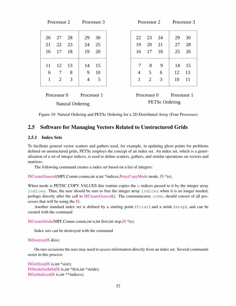
Processor 2 Processor 3
22 23 24 29 3026 27 28 29 30
Processor 2 Processor 3
21 22 23 24 25
16 17 18 19 20
11 12 13 14 15
6 7 8 9 10
1 2 3 4 5
19 20 21 27 28
16 17 18 25 26
Natural Ordering PETSc Ordering
Processor 1Processor 0Processor 1Processor 0
7 8 9 14 15
4 5 6 12 13
1 2 3 10 11
Figure 10: Natural Ordering and PETSc Ordering for a 2D Distributed Array (Four Processes)
2.5 Software for Managing Vectors Related to Unstructured Grids
2.5.1 Index Sets
To facilitate general vector scatters and gathers used, for example, in updating ghost points for problemsdefined on unstructured grids, PETSc employs the concept of an index set. An index set, which is a gener-alization of a set of integer indices, is used to define scatters, gathers, and similar operations on vectors andmatrices.
The following command creates a index set based on a list of integers:
ISCreateGeneral(MPI Comm comm,int n,int *indices,PetscCopyMode mode, IS *is);
When mode is PETSC COPY VALUES this routine copies the n indices passed to it by the integer arrayindices. Thus, the user should be sure to free the integer array indices when it is no longer needed,perhaps directly after the call to ISCreateGeneral(). The communicator, comm, should consist of all pro-cesses that will be using the IS.
Another standard index set is defined by a starting point (first) and a stride (step), and can becreated with the command
ISCreateStride(MPI Comm comm,int n,int first,int step,IS *is);
Index sets can be destroyed with the command
ISDestroy(IS &is);
On rare occasions the user may need to access information directly from an index set. Several commandsassist in this process:
ISGetSize(IS is,int *size);ISStrideGetInfo(IS is,int *first,int *stride);ISGetIndices(IS is,int **indices);
52
The function ISGetIndices() returns a pointer to a list of the indices in the index set. For certain index sets,this may be a temporary array of indices created specifically for a given routine. Thus, once the user finishesusing the array of indices, the routine
ISRestoreIndices(IS is, int **indices);
should be called to ensure that the system can free the space it may have used to generate the list of indices.A blocked version of the index sets can be created with the command
ISCreateBlock(MPI Comm comm,int bs,int n,int *indices,PetscCopyMode mode, IS *is);
This version is used for defining operations in which each element of the index set refers to a block ofbs vector entries. Related routines analogous to those described above exist as well, including ISBlock-GetIndices(), ISBlockGetSize(), ISBlockGetLocalSize(), ISGetBlockSize(). See the man pages for details.
2.5.2 Scatters and Gathers
PETSc vectors have full support for general scatters and gathers. One can select any subset of the com-ponents of a vector to insert or add to any subset of the components of another vector. We refer to theseoperations as generalized scatters, though they are actually a combination of scatters and gathers.
To copy selected components from one vector to another, one uses the following set of commands:
VecScatterCreate(Vec x,IS ix,Vec y,IS iy,VecScatter *ctx);VecScatterBegin(VecScatter ctx,Vec x,Vec y,INSERT VALUES,SCATTER FORWARD);VecScatterEnd(VecScatter ctx,Vec x,Vec y,INSERT VALUES,SCATTER FORWARD);VecScatterDestroy(VecScatter *ctx);
Here ix denotes the index set of the first vector, while iy indicates the index set of the destination vector.The vectors can be parallel or sequential. The only requirements are that the number of entries in the indexset of the first vector, ix, equal the number in the destination index set, iy, and that the vectors be longenough to contain all the indices referred to in the index sets. The argument INSERT VALUES specifiesthat the vector elements will be inserted into the specified locations of the destination vector, overwritingany existing values. To add the components, rather than insert them, the user should select the optionADD VALUES instead of INSERT VALUES.
To perform a conventional gather operation, the user simply makes the destination index set, iy, be astride index set with a stride of one. Similarly, a conventional scatter can be done with an initial (sending)index set consisting of a stride. The scatter rotines are collective operations (i.e. all processes that own aparallel vector must call the scatter routines). When scattering from a parallel vector to sequential vectors,each process has its own sequential vector that receives values from locations as indicated in its own indexset. Similarly, in scattering from sequential vectors to a parallel vector, each process has its own sequentialvector that makes contributions to the parallel vector.
Caution: When INSERT VALUES is used, if two different processes contribute different values to thesame component in a parallel vector, either value may end up being inserted. When ADD VALUES is used,the correct sum is added to the correct location.
In some cases one may wish to “undo” a scatter, that is perform the scatter backwards switching theroles of the sender and receiver. This is done by using
VecScatterBegin(VecScatter ctx,Vec y,Vec x,INSERT VALUES,SCATTER REVERSE);VecScatterEnd(VecScatter ctx,Vec y,Vec x,INSERT VALUES,SCATTER REVERSE);
Note that the roles of the first two arguments to these routines must be swapped whenever the SCAT-TER REVERSE option is used.
53
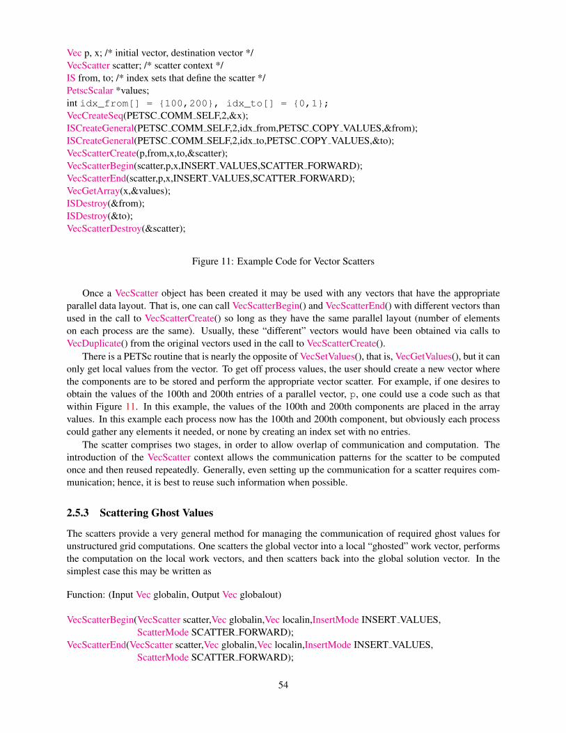
Vec p, x; /* initial vector, destination vector */VecScatter scatter; /* scatter context */IS from, to; /* index sets that define the scatter */PetscScalar *values;int idx_from[] = {100,200}, idx_to[] = {0,1};VecCreateSeq(PETSC COMM SELF,2,&x);ISCreateGeneral(PETSC COMM SELF,2,idx from,PETSC COPY VALUES,&from);ISCreateGeneral(PETSC COMM SELF,2,idx to,PETSC COPY VALUES,&to);VecScatterCreate(p,from,x,to,&scatter);VecScatterBegin(scatter,p,x,INSERT VALUES,SCATTER FORWARD);VecScatterEnd(scatter,p,x,INSERT VALUES,SCATTER FORWARD);VecGetArray(x,&values);ISDestroy(&from);ISDestroy(&to);VecScatterDestroy(&scatter);
Figure 11: Example Code for Vector Scatters
Once a VecScatter object has been created it may be used with any vectors that have the appropriateparallel data layout. That is, one can call VecScatterBegin() and VecScatterEnd() with different vectors thanused in the call to VecScatterCreate() so long as they have the same parallel layout (number of elementson each process are the same). Usually, these “different” vectors would have been obtained via calls toVecDuplicate() from the original vectors used in the call to VecScatterCreate().
There is a PETSc routine that is nearly the opposite of VecSetValues(), that is, VecGetValues(), but it canonly get local values from the vector. To get off process values, the user should create a new vector wherethe components are to be stored and perform the appropriate vector scatter. For example, if one desires toobtain the values of the 100th and 200th entries of a parallel vector, p, one could use a code such as thatwithin Figure 11. In this example, the values of the 100th and 200th components are placed in the arrayvalues. In this example each process now has the 100th and 200th component, but obviously each processcould gather any elements it needed, or none by creating an index set with no entries.
The scatter comprises two stages, in order to allow overlap of communication and computation. Theintroduction of the VecScatter context allows the communication patterns for the scatter to be computedonce and then reused repeatedly. Generally, even setting up the communication for a scatter requires com-munication; hence, it is best to reuse such information when possible.
2.5.3 Scattering Ghost Values
The scatters provide a very general method for managing the communication of required ghost values forunstructured grid computations. One scatters the global vector into a local “ghosted” work vector, performsthe computation on the local work vectors, and then scatters back into the global solution vector. In thesimplest case this may be written as
Function: (Input Vec globalin, Output Vec globalout)
VecScatterBegin(VecScatter scatter,Vec globalin,Vec localin,InsertMode INSERT VALUES,ScatterMode SCATTER FORWARD);
VecScatterEnd(VecScatter scatter,Vec globalin,Vec localin,InsertMode INSERT VALUES,ScatterMode SCATTER FORWARD);
54

/* For example, do local calculations from localin to localout */VecScatterBegin(VecScatter scatter,Vec localout,Vec globalout,InsertMode ADD VALUES,
ScatterMode SCATTER REVERSE);VecScatterEnd(VecScatter scatter,Vec localout,Vec globalout,InsertMode ADD VALUES,
ScatterMode SCATTER REVERSE);
2.5.4 Vectors with Locations for Ghost Values
There are two minor drawbacks to the basic approach described above:
• the extra memory requirement for the local work vector, localin, which duplicates the memory inglobalin, and
• the extra time required to copy the local values from localin to globalin.
An alternative approach is to allocate global vectors with space preallocated for the ghost values; thismay be done with either
VecCreateGhost(MPI Comm comm,int n,int N,int nghost,int *ghosts,Vec *vv)
or
VecCreateGhostWithArray(MPI Comm comm,int n,int N,int nghost,int *ghosts,PetscScalar *array,Vec *vv)
Here n is the number of local vector entries, N is the number of global entries (or PETSC NULL) andnghost is the number of ghost entries. The array ghosts is of size nghost and contains the globalvector location for each local ghost location. Using VecDuplicate() or VecDuplicateVecs() on a ghostedvector will generate additional ghosted vectors.
In many ways a ghosted vector behaves just like any other MPI vector created by VecCreateMPI(), thedifference is that the ghosted vector has an additional “local” representation that allows one to access theghost locations. This is done through the call to
VecGhostGetLocalForm(Vec g,Vec *l);
The vector l is a sequential representation of the parallel vector g that shares the same array space (andhence numerical values); but allows one to access the “ghost” values past “the end of the” array. Note thatone access the entries in l using the local numbering of elements and ghosts, while they are accessed in gusing the global numbering.
A common usage of a ghosted vector is given by
VecGhostUpdateBegin(Vec globalin,InsertMode INSERT VALUES,ScatterMode SCATTER FORWARD);
VecGhostUpdateEnd(Vec globalin,InsertMode INSERT VALUES,ScatterMode SCATTER FORWARD);
VecGhostGetLocalForm(Vec globalin,Vec *localin);VecGhostGetLocalForm(Vec globalout,Vec *localout);/*Do local calculations from localin to localout*/VecGhostRestoreLocalForm(Vec globalin,Vec *localin);VecGhostRestoreLocalForm(Vec globalout,Vec *localout);VecGhostUpdateBegin(Vec globalout,InsertMode ADD VALUES,
55

ScatterMode SCATTER REVERSE);VecGhostUpdateEnd(Vec globalout,InsertMode ADD VALUES,
ScatterMode SCATTER REVERSE);
The routines VecGhostUpdateBegin() and VecGhostUpdateEnd() are equivalent to the routines VecScat-terBegin() and VecScatterEnd() above except that since they are scattering into the ghost locations, they donot need to copy the local vector values, which are already in place. In addition, the user does not haveto allocate the local work vector, since the ghosted vector already has allocated slots to contain the ghostvalues.
The input arguments INSERT VALUES and SCATTER FORWARD cause the ghost values to be cor-rectly updated from the appropriate process. The arguments ADD VALUES and SCATTER REVERSEupdate the “local” portions of the vector from all the other processes’ ghost values. This would be appropri-ate, for example, when performing a finite element assembly of a load vector.
Section 3.5 discusses the important topic of partitioning an unstructured grid.
56
Chapter 3
Matrices
PETSc provides a variety of matrix implementations because no single matrix format is appropriate for allproblems. Currently we support dense storage and compressed sparse row storage (both sequential andparallel versions), as well as several specialized formats. Additional formats can be added.
This chapter describes the basics of using PETSc matrices in general (regardless of the particular formatchosen) and discusses tips for efficient use of the several simple uniprocess and parallel matrix types. Theuse of PETSc matrices involves the following actions: create a particular type of matrix, insert values into it,process the matrix, use the matrix for various computations, and finally destroy the matrix. The applicationcode does not need to know or care about the particular storage formats of the matrices.
3.1 Creating and Assembling Matrices
The simplest routine for forming a PETSc matrix, A, is followed by
MatCreate(MPI Comm comm,Mat *A) MatSetSizes(Mat A,int m,int n,int M,int N)
This routine generates a sequential matrix when running one process and a parallel matrix for two or moreprocesses; the particular matrix format is set by the user via options database commands. The user specifieseither the global matrix dimensions, given by M and N or the local dimensions, given by m and nwhile PETSccompletely controls memory allocation. This routine facilitates switching among various matrix types, forexample, to determine the format that is most efficient for a certain application. By default, MatCreate()employs the sparse AIJ format, which is discussed in detail Section 3.1.1. See the manual pages for furtherinformation about available matrix formats.
To insert or add entries to a matrix, one can call a variant of MatSetValues(), either
MatSetValues(Mat A,int m,const int idxm[],int n,const int idxn[],const PetscScalar values[],INSERT VALUES);
or
MatSetValues(Mat A,int m,const int idxm[],int n,const int idxn[],const PetscScalar values[],ADD VALUES);
This routine inserts or adds a logically dense subblock of dimension m*n into the matrix. The integer indicesidxm and idxn, respectively, indicate the global row and column numbers to be inserted. MatSetValues()uses the standard C convention, where the row and column matrix indices begin with zero regardless ofthe storage format employed. The array values is logically two-dimensional, containing the values thatare to be inserted. By default the values are given in row major order, which is the opposite of the For-tran convention, meaning that the value to be put in row idxm[i] and column idxn[j] is located invalues[i*n+j]. To allow the insertion of values in column major order, one can call the command
57
MatSetOption(Mat A,MAT COLUMN ORIENTED,PETSC TRUE);
Warning: Several of the sparse implementations do not currently support the column-oriented option.This notation should not be a mystery to anyone. For example, to insert one matrix into another when
using MATLAB, one uses the command A(im,in) = B; where im and in contain the indices for therows and columns. This action is identical to the calls above to MatSetValues().
When using the block compressed sparse row matrix format (MATSEQBAIJ or MATMPIBAIJ), one caninsert elements more efficiently using the block variant, MatSetValuesBlocked() or MatSetValuesBlocked-Local().
The function MatSetOption() accepts several other inputs; see the manual page for details.After the matrix elements have been inserted or added into the matrix, they must be processed (also
called assembled) before they can be used. The routines for matrix processing are
MatAssemblyBegin(Mat A,MAT FINAL ASSEMBLY);MatAssemblyEnd(Mat A,MAT FINAL ASSEMBLY);
By placing other code between these two calls, the user can perform computations while messages are intransit. Calls to MatSetValues() with the INSERT VALUES and ADD VALUES options cannot be mixedwithout intervening calls to the assembly routines. For such intermediate assembly calls the second routineargument typically should be MAT_FLUSH_ASSEMBLY, which omits some of the work of the full assemblyprocess. MAT_FINAL_ASSEMBLY is required only in the last matrix assembly before a matrix is used.
Even though one may insert values into PETSc matrices without regard to which process eventuallystores them, for efficiency reasons we usually recommend generating most entries on the process wherethey are destined to be stored. To help the application programmer with this task for matrices that aredistributed across the processes by ranges, the routine
MatGetOwnershipRange(Mat A,int *first row,int *last row);
informs the user that all rows from first_row to last_row-1 (since the value returned in last_rowis one more than the global index of the last local row) will be stored on the local process.
In the sparse matrix implementations, once the assembly routines have been called, the matrices arecompressed and can be used for matrix-vector multiplication, etc. Inserting new values into the matrixat this point will be expensive, since it requires copies and possible memory allocation. Thus, wheneverpossible one should completely set the values in the matrices before calling the final assembly routines.
If one wishes to repeatedly assemble matrices that retain the same nonzero pattern (such as within anonlinear or time-dependent problem), the option
MatSetOption(Mat A,MAT NO NEW NONZERO LOCATIONS,PETSC TRUE);
should be specified after the first matrix has been fully assembled. This option ensures that certain datastructures and communication information will be reused (instead of regenerated) during successive steps,thereby increasing efficiency. See ${PETSC_DIR}/src/ksp/ksp/examples/tutorials/ex5.c for a simple example of solving two linear systems that use the same matrix data structure.
3.1.1 Sparse Matrices
The default matrix representation within PETSc is the general sparse AIJ format (also called the Yale sparsematrix format or compressed sparse row format, CSR). This section discusses tips for efficiently using thismatrix format for large-scale applications. Additional formats (such as block compressed row and blockdiagonal storage, which are generally much more efficient for problems with multiple degrees of freedomper node) are discussed below. Beginning users need not concern themselves initially with such details andmay wish to proceed directly to Section 3.2. However, when an application code progresses to the point oftuning for efficiency and/or generating timing results, it is crucial to read this information.
58
Sequential AIJ Sparse Matrices
In the PETSc AIJ matrix formats, we store the nonzero elements by rows, along with an array of correspond-ing column numbers and an array of pointers to the beginning of each row. Note that the diagonal matrixentries are stored with the rest of the nonzeros (not separately).
To create a sequential AIJ sparse matrix, A, with m rows and n columns, one uses the command
MatCreateSeqAIJ(PETSC COMM SELF,int m,int n,int nz,int *nnz,Mat *A);
where nz or nnz can be used to preallocate matrix memory, as discussed below. The user can set nz=0and nnz=PETSC NULL for PETSc to control all matrix memory allocation.
The sequential and parallel AIJ matrix storage formats by default employ i-nodes (identical nodes)when possible. We search for consecutive rows with the same nonzero structure, thereby reusing matrixinformation for increased efficiency. Related options database keys are -mat_no_inode (do not useinodes) and -mat_inode_limit <limit> (set inode limit (max limit=5)). Note that problems witha single degree of freedom per grid node will automatically not use I-nodes.
By default the internal data representation for the AIJ formats employs zero-based indexing. For com-patibility with standard Fortran storage, thus enabling use of external Fortran software packages such asSPARSKIT, the option -mat_aij_oneindex enables one-based indexing, where the stored row andcolumn indices begin at one, not zero. All user calls to PETSc routines, regardless of this option, usezero-based indexing.
Preallocation of Memory for Sequential AIJ Sparse Matrices
The dynamic process of allocating new memory and copying from the old storage to the new is intrinsicallyvery expensive. Thus, to obtain good performance when assembling an AIJ matrix, it is crucial to preallocatethe memory needed for the sparse matrix. The user has two choices for preallocating matrix memory viaMatCreateSeqAIJ().
One can use the scalar nz to specify the expected number of nonzeros for each row. This is generallyfine if the number of nonzeros per row is roughly the same throughout the matrix (or as a quick and easy firststep for preallocation). If one underestimates the actual number of nonzeros in a given row, then during theassembly process PETSc will automatically allocate additional needed space. However, this extra memoryallocation can slow the computation,
If different rows have very different numbers of nonzeros, one should attempt to indicate (nearly) theexact number of elements intended for the various rows with the optional array, nnz of length m, where m isthe number of rows, for example
int nnz[m];nnz[0] = <nonzeros in row 0>nnz[1] = <nonzeros in row 1>....nnz[m-1] = <nonzeros in row m-1>
In this case, the assembly process will require no additional memory allocations if the nnz estimates arecorrect. If, however, the nnz estimates are incorrect, PETSc will automatically obtain the additional neededspace, at a slight loss of efficiency.
Using the array nnz to preallocate memory is especially important for efficient matrix assembly if thenumber of nonzeros varies considerably among the rows. One can generally set nnz either by knowingin advance the problem structure (e.g., the stencil for finite difference problems on a structured grid) or byprecomputing the information by using a segment of code similar to that for the regular matrix assembly.The overhead of determining the nnz array will be quite small compared with the overhead of the inherently
59

expensive mallocs and moves of data that are needed for dynamic allocation during matrix assembly. Alwaysguess high if exact value is not known (since extra space is cheaper than too little).
Thus, when assembling a sparse matrix with very different numbers of nonzeros in various rows, onecould proceed as follows for finite difference methods:
- Allocate integer array nnz.- Loop over grid, counting the expected number of nonzeros for the row(s)
associated with the various grid points.- Create the sparse matrix via MatCreateSeqAIJ() or alternative.- Loop over the grid, generating matrix entries and inserting in matrix via MatSetValues().
For (vertex-based) finite element type calculations, an analogous procedure is as follows:
- Allocate integer array nnz.- Loop over vertices, computing the number of neighbor vertices, which determines the
number of nonzeros for the corresponding matrix row(s).- Create the sparse matrix via MatCreateSeqAIJ() or alternative.- Loop over elements, generating matrix entries and inserting in matrix via MatSetValues().
The -info option causes the routines MatAssemblyBegin() and MatAssemblyEnd() to print informa-tion about the success of the preallocation. Consider the following example for the MATSEQAIJ matrixformat:
MatAssemblyEnd SeqAIJ:Matrix size 10 X 10; storage space:20 unneeded, 100 usedMatAssemblyEnd SeqAIJ:Number of mallocs during MatSetValues is 0
The first line indicates that the user preallocated 120 spaces but only 100 were used. The second lineindicates that the user preallocated enough space so that PETSc did not have to internally allocate additionalspace (an expensive operation). In the next example the user did not preallocate sufficient space, as indicatedby the fact that the number of mallocs is very large (bad for efficiency):
MatAssemblyEnd SeqAIJ:Matrix size 10 X 10; storage space:47 unneeded, 1000 usedMatAssemblyEnd SeqAIJ:Number of mallocs during MatSetValues is 40000
Although at first glance such procedures for determining the matrix structure in advance may seemunusual, they are actually very efficient because they alleviate the need for dynamic construction of thematrix data structure, which can be very expensive.
Parallel AIJ Sparse Matrices
Parallel sparse matrices with the AIJ format can be created with the command
MatCreateMPIAIJ(MPI Comm comm,int m,int n,int M,int N,int d nz,int *d nnz, int o nz,int *o nnz,Mat *A);
A is the newly created matrix, while the arguments m, M, and N, indicate the number of local rows andthe number of global rows and columns, respectively. In the PETSc partitioning scheme, all the matrixcolumns are local and n is the number of columns corresponding to local part of a parallel vector. Either thelocal or global parameters can be replaced with PETSC DECIDE, so that PETSc will determine them. Thematrix is stored with a fixed number of rows on each process, given by m, or determined by PETSc if m isPETSC DECIDE.
60
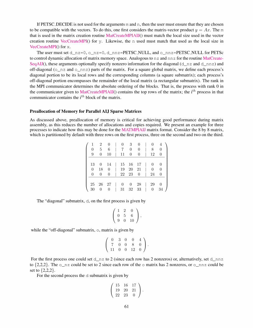
If PETSC DECIDE is not used for the arguments m and n, then the user must ensure that they are chosento be compatible with the vectors. To do this, one first considers the matrix-vector product y = Ax. The mthat is used in the matrix creation routine MatCreateMPIAIJ() must match the local size used in the vectorcreation routine VecCreateMPI() for y. Likewise, the n used must match that used as the local size inVecCreateMPI() for x.
The user must set d_nz=0, o_nz=0, d_nnz=PETSC NULL, and o_nnz=PETSC NULL for PETScto control dynamic allocation of matrix memory space. Analogous to nz and nnz for the routine MatCreate-SeqAIJ(), these arguments optionally specify nonzero information for the diagonal (d_nz and d_nnz) andoff-diagonal (o_nz and o_nnz) parts of the matrix. For a square global matrix, we define each process’sdiagonal portion to be its local rows and the corresponding columns (a square submatrix); each process’soff-diagonal portion encompasses the remainder of the local matrix (a rectangular submatrix). The rank inthe MPI communicator determines the absolute ordering of the blocks. That is, the process with rank 0 inthe communicator given to MatCreateMPIAIJ() contains the top rows of the matrix; the ith process in thatcommunicator contains the ith block of the matrix.
Preallocation of Memory for Parallel AIJ Sparse Matrices
As discussed above, preallocation of memory is critical for achieving good performance during matrixassembly, as this reduces the number of allocations and copies required. We present an example for threeprocesses to indicate how this may be done for the MATMPIAIJ matrix format. Consider the 8 by 8 matrix,which is partitioned by default with three rows on the first process, three on the second and two on the third.
1 2 0 | 0 3 0 | 0 40 5 6 | 7 0 0 | 8 09 0 10 | 11 0 0 | 12 0
13 0 14 | 15 16 17 | 0 00 18 0 | 19 20 21 | 0 00 0 0 | 22 23 0 | 24 0
25 26 27 | 0 0 28 | 29 030 0 0 | 31 32 33 | 0 34
The “diagonal” submatrix, d, on the first process is given by 1 2 0
0 5 69 0 10
,
while the “off-diagonal” submatrix, o, matrix is given by 0 3 0 0 47 0 0 8 011 0 0 12 0
.
For the first process one could set d_nz to 2 (since each row has 2 nonzeros) or, alternatively, set d_nnzto {2,2,2}. The o_nz could be set to 2 since each row of the o matrix has 2 nonzeros, or o_nnz could beset to {2,2,2}.
For the second process the d submatrix is given by 15 16 1719 20 2122 23 0
.
61
Thus, one could set d_nz to 3, since the maximum number of nonzeros in each row is 3, or alternativelyone could set d_nnz to {3,3,2}, thereby indicating that the first two rows will have 3 nonzeros while thethird has 2. The corresponding o submatrix for the second process is 13 0 14 0 0
0 18 0 0 00 0 0 24 0
so that one could set o_nz to 2 or o_nnz to {2,1,1}.
Note that the user never directly works with the d and o submatrices, except when preallocating storagespace as indicated above. Also, the user need not preallocate exactly the correct amount of space; as long asa sufficiently close estimate is given, the high efficiency for matrix assembly will remain.
As described above, the option -info will print information about the success of preallocation duringmatrix assembly. For the MATMPIAIJ and MATMPIBAIJ formats, PETSc will also list the number ofelements owned by on each process that were generated on a different process. For example, the statements
MatAssemblyBegin MPIAIJ:Stash has 10 entries, uses 0 mallocsMatAssemblyBegin MPIAIJ:Stash has 3 entries, uses 0 mallocsMatAssemblyBegin MPIAIJ:Stash has 5 entries, uses 0 mallocs
indicate that very few values have been generated on different processes. On the other hand, the statements
MatAssemblyBegin MPIAIJ:Stash has 100000 entries, uses 100 mallocsMatAssemblyBegin MPIAIJ:Stash has 77777 entries, uses 70 mallocs
indicate that many values have been generated on the “wrong” processes. This situation can be very inef-ficient, since the transfer of values to the “correct” process is generally expensive. By using the commandMatGetOwnershipRange() in application codes, the user should be able to generate most entries on theowning process.
Note: It is fine to generate some entries on the “wrong” process. Often this can lead to cleaner, simpler,less buggy codes. One should never make code overly complicated in order to generate all values locally.Rather, one should organize the code in such a way that most values are generated locally.
3.1.2 Dense Matrices
PETSc provides both sequential and parallel dense matrix formats, where each process stores its entries in acolumn-major array in the usual Fortran style. To create a sequential, dense PETSc matrix, A of dimensionsm by n, the user should call
MatCreateSeqDense(PETSC COMM SELF,int m,int n,PetscScalar *data,Mat *A);
The variable data enables the user to optionally provide the location of the data for matrix storage (intendedfor Fortran users who wish to allocate their own storage space). Most users should merely set data toPETSC NULL for PETSc to control matrix memory allocation. To create a parallel, dense matrix, A, theuser should call
MatCreateMPIDense(MPI Comm comm,int m,int n,int M,int N,PetscScalar *data,Mat *A)
The arguments m, n, M, and N, indicate the number of local rows and columns and the number of global rowsand columns, respectively. Either the local or global parameters can be replaced with PETSC DECIDE, sothat PETSc will determine them. The matrix is stored with a fixed number of rows on each process, givenby m, or determined by PETSc if m is PETSC DECIDE.
PETSc does not provide parallel dense direct solvers. Our focus is on sparse iterative solvers.
62
3.1.3 Block Matrices
Block matrices arise when coupling variables with different meaning, especially when solving problemswith constraints (e.g. incompressible flow) and “multi-physics” problems. Usually the number of blocks issmall and each block is partitioned in parallel. We illustrate for a 3 × 3 system with components labeleda, b, c. With some numbering of unknowns, the matrix could be written as Aaa Aab Aac
Aba Abb Abc
Aca Acb Acc
.There are two fundamentally different ways that this matrix could be stored, as a single assembled sparsematrix where entries from all blocks are merged together (“monolithic”), or as separate assembled matri-ces for each block (“nested”). These formats have different performance characteristics depending on theoperation being performed. In particular, many preconditioners require a monolithic format, but some thatare very effective for solving block systems (see Section 4.5) are more efficient when a nested format isused. In order to stay flexible, we would like to be able to use the same code to assemble block matrices inboth monolithic and nested formats. Additionally, for software maintainability and testing, especially in amulti-physics context where different groups might be responsible for assembling each of the blocks, it isdesirable to be able to use exactly the same code to assemble a single block independently as to assemble itas part of a larger system. To do this, we introduce the four spaces shown in Figure 12.
• The monolithic global space is the space in which the Krylov and Newton solvers operate, withcollective semantics across the entire block system.
• The split global space splits the blocks apart, but each split still has collective semantics.
• The split local space adds ghost points and sperates the blocks. Operations in this space can beperformed with no parallel communication. This is often the most natural, and certainly the mostpowerful, space for matrix assembly code.
• The monolithic local space can be thought of as adding ghost points to the monolithic global space,but it is often more natural to use it simply as a concatenation of split local spaces on each process. Itis not common to explicitly manipulate vectors or matrices in this space (at least not during assembly),but it is a useful for declaring which part of a matrix is being assembled.
The key to format-independent assembly is the function
MatGetLocalSubMatrix(Mat A,IS isrow,IS iscol,Mat *submat);
which provides a “view” submat into a matrix A that operates in the monolithic global space. The submattransforms from the split local space defined by iscol to the split local space defined by isrow. The indexsets specify the parts of the monolithic local space that submat should operate in. If a nested matrix formatis used, then MatGetLocalSubMatrix() finds the nested block and returns it without making any copies. Inthis case, submat is fully functional and has a parallel communicator. If a monolithic matrix format is used,then MatGetLocalSubMatrix() returns a proxy matrix on PETSC_COMM_SELF that does not provide valuesor implement MatMult(), but does implement MatSetValuesLocal() and, if isrow,iscol have a constantblock size, MatSetValuesBlockedLocal(). Note that although submat may not be a fully functional matrixand the caller does not even know a priori which communicator it will reside on, it always implements thelocal assembly functions (which are not collective). The index sets isrow,iscol can be obtained usingDMCompositeGetLocalISs() if DMComposite is being used. DMComposite can also be used to creatematrices, in which case the MATNEST format can be specified using -prefix_dm_mat_type nestand MATAIJ can be specified using -prefix_dm_mat_type aij. See $PETSC_DIR/src/snes/examples/tutorials/ex28.c for a simple example using this interface.
63
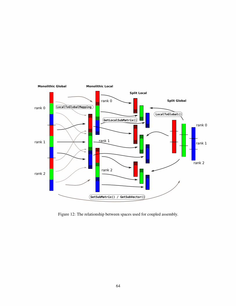
rank 0
rank 2
rank 1
rank 0
rank 1
rank 2
LocalToGlobalMapping
Monolithic Global Monolithic Local
Split Local
GetLocalSubMatrix()
Split Global
GetSubMatrix() / GetSubVector()
LocalToGlobal()
rank 0
rank 1
rank 2
Figure 12: The relationship between spaces used for coupled assembly.
64
3.2 Basic Matrix Operations
Table 2 summarizes basic PETSc matrix operations. We briefly discuss a few of these routines in more detailbelow.
The parallel matrix can multiply a vector with n local entries, returning a vector with m local entries.That is, to form the product
MatMult(Mat A,Vec x,Vec y);
the vectors x and y should be generated with
VecCreateMPI(MPI Comm comm,n,N,&x);VecCreateMPI(MPI Comm comm,m,M,&y);
By default, if the user lets PETSc decide the number of components to be stored locally (by passing inPETSC DECIDE as the second argument to VecCreateMPI() or using VecCreate()), vectors and matrices ofthe same dimension are automatically compatible for parallel matrix-vector operations.
Along with the matrix-vector multiplication routine, there is a version for the transpose of the matrix,
MatMultTranspose(Mat A,Vec x,Vec y);
There are also versions that add the result to another vector:
MatMultAdd(Mat A,Vec x,Vec y,Vec w);MatMultTransposeAdd(Mat A,Vec x,Vec y,Vec w);
These routines, respectively, produce w = A ∗ x + y and w = AT ∗ x + y . In C it is legal for the vectorsy and w to be identical. In Fortran, this situation is forbidden by the language standard, but we allow itanyway.
One can print a matrix (sequential or parallel) to the screen with the command
MatView(Mat mat,PETSC VIEWER STDOUT WORLD);
Other viewers can be used as well. For instance, one can draw the nonzero stucture of the matrix into thedefault X-window with the command
MatView(Mat mat,PETSC VIEWER DRAW WORLD);
Also one can use
MatView(Mat mat,PetscViewer viewer);
where viewer was obtained with PetscViewerDrawOpen(). Additional viewers and options are given inthe MatView() man page and Section 13.3.
The NormType argument to MatNorm() is one of NORM 1, NORM INFINITY, and NORM FROBENIUS.
3.3 Matrix-Free Matrices
Some people like to use matrix-free methods, which do not require explicit storage of the matrix, for thenumerical solution of partial differential equations. To support matrix-free methods in PETSc, one can usethe following command to create a Mat structure without ever actually generating the matrix:
MatCreateShell(MPI Comm comm,int m,int n,int M,int N,void *ctx,Mat *mat);
65
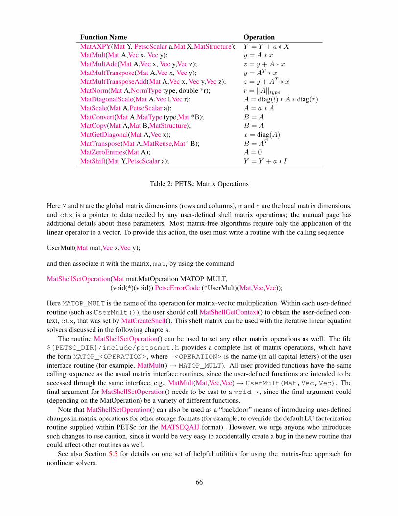
Function Name OperationMatAXPY(Mat Y, PetscScalar a,Mat X,MatStructure); Y = Y + a ∗XMatMult(Mat A,Vec x, Vec y); y = A ∗ xMatMultAdd(Mat A,Vec x, Vec y,Vec z); z = y +A ∗ xMatMultTranspose(Mat A,Vec x, Vec y); y = AT ∗ xMatMultTransposeAdd(Mat A,Vec x, Vec y,Vec z); z = y +AT ∗ xMatNorm(Mat A,NormType type, double *r); r = ||A||type
MatDiagonalScale(Mat A,Vec l,Vec r); A = diag(l) ∗A ∗ diag(r)MatScale(Mat A,PetscScalar a); A = a ∗AMatConvert(Mat A,MatType type,Mat *B); B = AMatCopy(Mat A,Mat B,MatStructure); B = AMatGetDiagonal(Mat A,Vec x); x = diag(A)MatTranspose(Mat A,MatReuse,Mat* B); B = AT
MatZeroEntries(Mat A); A = 0MatShift(Mat Y,PetscScalar a); Y = Y + a ∗ I
Table 2: PETSc Matrix Operations
Here M and N are the global matrix dimensions (rows and columns), m and n are the local matrix dimensions,and ctx is a pointer to data needed by any user-defined shell matrix operations; the manual page hasadditional details about these parameters. Most matrix-free algorithms require only the application of thelinear operator to a vector. To provide this action, the user must write a routine with the calling sequence
UserMult(Mat mat,Vec x,Vec y);
and then associate it with the matrix, mat, by using the command
MatShellSetOperation(Mat mat,MatOperation MATOP MULT,(void(*)(void)) PetscErrorCode (*UserMult)(Mat,Vec,Vec));
Here MATOP_MULT is the name of the operation for matrix-vector multiplication. Within each user-definedroutine (such as UserMult()), the user should call MatShellGetContext() to obtain the user-defined con-text, ctx, that was set by MatCreateShell(). This shell matrix can be used with the iterative linear equationsolvers discussed in the following chapters.
The routine MatShellSetOperation() can be used to set any other matrix operations as well. The file${PETSC_DIR}/include/petscmat.h provides a complete list of matrix operations, which havethe form MATOP_<OPERATION>, where <OPERATION> is the name (in all capital letters) of the userinterface routine (for example, MatMult() → MATOP_MULT). All user-provided functions have the samecalling sequence as the usual matrix interface routines, since the user-defined functions are intended to beaccessed through the same interface, e.g., MatMult(Mat,Vec,Vec)→ UserMult(Mat,Vec,Vec). Thefinal argument for MatShellSetOperation() needs to be cast to a void *, since the final argument could(depending on the MatOperation) be a variety of different functions.
Note that MatShellSetOperation() can also be used as a “backdoor” means of introducing user-definedchanges in matrix operations for other storage formats (for example, to override the default LU factorizationroutine supplied within PETSc for the MATSEQAIJ format). However, we urge anyone who introducessuch changes to use caution, since it would be very easy to accidentally create a bug in the new routine thatcould affect other routines as well.
See also Section 5.5 for details on one set of helpful utilities for using the matrix-free approach fornonlinear solvers.
66
3.4 Other Matrix Operations
In many iterative calculations (for instance, in a nonlinear equations solver), it is important for efficiencypurposes to reuse the nonzero structure of a matrix, rather than determining it anew every time the matrix isgenerated. To retain a given matrix but reinitialize its contents, one can employ
MatZeroEntries(Mat A);
This routine will zero the matrix entries in the data structure but keep all the data that indicates where thenonzeros are located. In this way a new matrix assembly will be much less expensive, since no memoryallocations or copies will be needed. Of course, one can also explicitly set selected matrix elements to zeroby calling MatSetValues().
By default, if new entries are made in locations where no nonzeros previously existed, space will beallocated for the new entries. To prevent the allocation of additional memory and simply discard those newentries, one can use the option
MatSetOption(Mat A,MAT NO NEW NONZERO LOCATIONS,PETSC TRUE);
Once the matrix has been assembled, one can factor it numerically without repeating the ordering or thesymbolic factorization. This option can save some computational time, although it does require that thefactorization is not done in-place.
In the numerical solution of elliptic partial differential equations, it can be cumbersome to deal withDirichlet boundary conditions. In particular, one would like to assemble the matrix without regard to bound-ary conditions and then at the end apply the Dirichlet boundary conditions. In numerical analysis classes thisprocess is usually presented as moving the known boundary conditions to the right-hand side and then solv-ing a smaller linear system for the interior unknowns. Unfortunately, implementing this requires extractinga large submatrix from the original matrix and creating its corresponding data structures. This process canbe expensive in terms of both time and memory.
One simple way to deal with this difficulty is to replace those rows in the matrix associated with knownboundary conditions, by rows of the identity matrix (or some scaling of it). This action can be done with thecommand
MatZeroRows(Mat A,PetscInt numRows,PetscInt rows[],PetscScalar diag value,Vec x,Vec b),
or equivalently,
MatZeroRowsIS(Mat A,IS rows,PetscScalar diag value,Vec x,Vec b);
For sparse matrices this removes the data structures for certain rows of the matrix. If the pointer diag_value is PETSC NULL, it even removes the diagonal entry. If the pointer is not null, it uses that givenvalue at the pointer location in the diagonal entry of the eliminated rows.
One nice feature of this approach is that when solving a nonlinear problem such that at each iteration theDirichlet boundary conditions are in the same positions and the matrix retains the same nonzero structure,the user can call MatZeroRows() in the first iteration. Then, before generating the matrix in the seconditeration the user should call
MatSetOption(Mat A,MAT NO NEW NONZERO LOCATIONS,PETSC TRUE);
From that point, no new values will be inserted into those (boundary) rows of the matrix.The functions MatZeroRowsLocal() and MatZeroRowsLocalIS() can also be used if for each process
one provides the Dirichlet locations in the local numbering of the matrix. A drawback of MatZeroRows() isthat it destroys the symmetry of a matrix. Thus one can use
67
MatZeroRowsColumns(Mat A,PetscInt numRows,PetscInt rows[],PetscScalar diag value,Vec x,Vec b),
or equivalently,
MatZeroRowsColumnsIS(Mat A,IS rows,PetscScalar diag value,Vec x,Vec b);
Note that with all of these for a given assembled matrix it can be only called once to update the x and bvector. It cannot be used if one wishes to solve multiple right hand side problems for the same matrix sincethe matrix entries needed for updating the b vector are removed in its first use.
Once the zeroed rows are removed the new matrix has possibly many rows with only a diagonal entryaffecting the parallel load balancing. The PCREDISTRIBUTE preconditioner removes all the zeroed rows(and associated columns and adjusts the right hand side based on the removed columns) and then rebalancesthe resulting rows of smaller matrix across the processes. Thus one can use MatZeroRows() to set theDirichlet points and then solve with the preconditioner PCREDISTRIBUTE. Note if the original matrix wassymmetric the smaller solved matrix will also be symmetric.
Another matrix routine of interest is
MatConvert(Mat mat,MatType newtype,Mat *M)
which converts the matrix mat to new matrix, M, that has either the same or different format. Set newtypeto MATSAME to copy the matrix, keeping the same matrix format. See ${PETSC_DIR}/include/petscmat.h for other available matrix types; standard ones are MATSEQDENSE, MATSEQAIJ, MATMPIAIJ,MATSEQBAIJ and MATMPIBAIJ.
In certain applications it may be necessary for application codes to directly access elements of a matrix.This may be done by using the the command (for local rows only)
MatGetRow(Mat A,int row, int *ncols,const PetscInt (*cols)[],const PetscScalar (*vals)[]);
The argument ncols returns the number of nonzeros in that row, while cols and vals returns the columnindices (with indices starting at zero) and values in the row. If only the column indices are needed (andnot the corresponding matrix elements), one can use PETSC NULL for the vals argument. Similarly,one can use PETSC NULL for the cols argument. The user can only examine the values extracted withMatGetRow(); the values cannot be altered. To change the matrix entries, one must use MatSetValues().
Once the user has finished using a row, he or she must call
MatRestoreRow(Mat A,int row,int *ncols,int **cols,PetscScalar **vals);
to free any space that was allocated during the call to MatGetRow().
3.5 Partitioning
For almost all unstructured grid computation, the distribution of portions of the grid across the process’swork load and memory can have a very large impact on performance. In most PDE calculations the gridpartitioning and distribution across the processes can (and should) be done in a “pre-processing” step beforethe numerical computations. However, this does not mean it need be done in a separate, sequential program,rather it should be done before one sets up the parallel grid data structures in the actual program. PETSc pro-vides an interface to the ParMETIS (developed by George Karypis; see the docs/installation/index.htm filefor directions on installing PETSc to use ParMETIS) to allow the partitioning to be done in parallel. PETScdoes not currently provide directly support for dynamic repartitioning, load balancing by migrating matrixentries between processes, etc. For problems that require mesh refinement, PETSc uses the “rebuild the datastructure” approach, as opposed to the “maintain dynamic data structures that support the insertion/deletionof additional vector and matrix rows and columns entries” approach.
68

Partitioning in PETSc is organized around the MatPartitioning object. One first creates a parallel matrixthat contains the connectivity information about the grid (or other graph-type object) that is to be partitioned.This is done with the command
MatCreateMPIAdj(MPI Comm comm,int mlocal,int n,const int ia[],const int ja[],int *weights,Mat *Adj);
The argument mlocal indicates the number of rows of the graph being provided by the given process, n isthe total number of columns; equal to the sum of all the mlocal. The arguments ia and ja are the rowpointers and column pointers for the given rows, these are the usual format for parallel compressed sparserow storage, using indices starting at 0, not 1.
1
2 3
4
5
0
0
12
3
Figure 13: Numbering on Simple Unstructured Grid
This, of course, assumes that one has already distributed the grid (graph) information among the pro-cesses. The details of this initial distribution is not important; it could be simply determined by assigning tothe first process the first n0 nodes from a file, the second process the next n1 nodes, etc.
For example, we demonstrate the form of the ia and ja for a triangular grid where we(1) partition by element (triangle)
• Process 0, mlocal = 2, n = 4, ja = {2, 3, |3}, ia = {0, 2, 3}
• Process 1, mlocal = 2, n = 4, ja = {0, |0, 1}, ia = {0, 1, 3}
Note that elements are not connected to themselves and we only indicate edge connections (in some contextssingle vertex connections between elements may also be included). We use a | above to denote the transitionbetween rows in the matrix.
and (2) partition by vertex.
• Process 0, mlocal = 3, n = 6, ja = {3, 4, |4, 5, |3, 4, 5}, ia = {0, 2, 4, 7}
• Process 1, mlocal = 3, n = 6, ja = {0, 2, 4, |0, 1, 2, 3, 5, |1, 2, 4}, ia = {0, 3, 8, 11}.
Once the connectivity matrix has been created the following code will generate the renumbering requiredfor the new partition
69

MatPartitioningCreate(MPI Comm comm,MatPartitioning *part);MatPartitioningSetAdjacency(MatPartitioning part,Mat Adj);MatPartitioningSetFromOptions(MatPartitioning part);MatPartitioningApply(MatPartitioning part,IS *is);MatPartitioningDestroy(MatPartitioning *part);MatDestroy(Mat *Adj);ISPartitioningToNumbering(IS is,IS *isg);
The resulting isg contains for each local node the new global number of that node. The resulting iscontains the new process number that each local node has been assigned to.
Now that a new numbering of the nodes has been determined one must renumber all the nodes andmigrate the grid information to the correct process. The command
AOCreateBasicIS(isg,PETSC NULL,&ao);
generates, see Section 2.3.1, an AO object that can be used in conjunction with the is and gis to move therelevant grid information to the correct process and renumber the nodes etc.
PETSc does not currently provide tools that completely manage the migration and node renumbering,since it will be dependent on the particular data structure you use to store the grid information and the typeof grid information that you need for your application. We do plan to include more support for this in thefuture, but designing the appropriate general user interface and providing a scalable implementation that canbe used for a wide variety of different grids requires a great deal of time.
70
Chapter 4
KSP: Linear Equations Solvers
The object KSP is the heart of PETSc, because it provides uniform and efficient access to all of the package’slinear system solvers, including parallel and sequential, direct and iterative. KSP is intended for solvingnonsingular systems of the form
Ax = b, (4.1)
where A denotes the matrix representation of a linear operator, b is the right-hand-side vector, and x is thesolution vector. KSP uses the same calling sequence for both direct and iterative solution of a linear system.In addition, particular solution techniques and their associated options can be selected at runtime.
The combination of a Krylov subspace method and a preconditioner is at the center of most modernnumerical codes for the iterative solution of linear systems. See, for example, [7] for an overview of thetheory of such methods. KSP creates a simplified interface to the lower-level KSP and PC modules withinthe PETSc package. The KSP package, discussed in Section 4.3, provides many popular Krylov subspaceiterative methods; the PC module, described in Section 4.4, includes a variety of preconditioners. Althoughboth KSP and PC can be used directly, users should employ the interface of KSP.
4.1 Using KSP
To solve a linear system with KSP, one must first create a solver context with the command
KSPCreate(MPI Comm comm,KSP *ksp);
Here comm is the MPI communicator, and ksp is the newly formed solver context. Before actually solvinga linear system with KSP, the user must call the following routine to set the matrices associated with thelinear system:
KSPSetOperators(KSP ksp,Mat Amat,Mat Pmat,MatStructure flag);
The argument Amat, representing the matrix that defines the linear system, is a symbolic place holder forany kind of matrix. In particular, KSP does support matrix-free methods. The routine MatCreateShell()in Section 3.3 provides further information regarding matrix-free methods. Typically the preconditioningmatrix (i.e., the matrix from which the preconditioner is to be constructed), Pmat, is the same as the matrixthat defines the linear system, Amat; however, occasionally these matrices differ (for instance, when apreconditioning matrix is obtained from a lower order method than that employed to form the linear systemmatrix). The argument flag can be used to eliminate unnecessary work when repeatedly solving linearsystems of the same size with the same preconditioning method; when solving just one linear system, thisflag is ignored. The user can set flag as follows:
71
• SAME_NONZERO_PATTERN - the preconditioning matrix has the same nonzero structure duringsuccessive linear solves,
• DIFFERENT_NONZERO_PATTERN - the preconditioning matrix does not have the same nonzerostructure during successive linear solves,
• SAME_PRECONDITIONER - the preconditioner matrix is identical to that of the previous linear solve.
If the structure of a matrix is not known a priori, one should use the flag DIFFERENT_NONZERO_PATTERN.
Much of the power of KSP can be accessed through the single routine
KSPSetFromOptions(KSP ksp);
This routine accepts the options -h and -help as well as any of the KSP and PC options discussed below.To solve a linear system, one sets the rhs and solution vectors using and executes the command
KSPSolve(KSP ksp,Vec b,Vec x);
where b and x respectively denote the right-hand-side and solution vectors. On return, the iteration numberat which the iterative process stopped can be obtained using
KSPGetIterationNumber(KSP ksp, int *its);
Note that this does not state that the method converged at this iteration: it can also have reached the maxi-mum number of iterations, or have diverged. Section 4.3.2 gives more details regarding convergence testing.Note that multiple linear solves can be performed by the same KSP context. Once the KSP context is nolonger needed, it should be destroyed with the command
KSPDestroy(KSP *ksp);
The above procedure is sufficient for general use of the KSP package. One additional step is required forusers who wish to customize certain preconditioners (e.g., see Section 4.4.4) or to log certain performancedata using the PETSc profiling facilities (as discussed in Chapter 11). In this case, the user can optionallyexplicitly call
KSPSetUp(KSP ksp)
before calling KSPSolve() to perform any setup required for the linear solvers. The explicit call of thisroutine enables the separate monitoring of any computations performed during the set up phase, such asincomplete factorization for the ILU preconditioner.
The default solver within KSP is restarted GMRES, preconditioned for the uniprocess case with ILU(0),and for the multiprocess case with the block Jacobi method (with one block per process, each of whichis solved with ILU(0)). A variety of other solvers and options are also available. To allow applicationprogrammers to set any of the preconditioner or Krylov subspace options directly within the code, weprovide routines that extract the PC and KSP contexts,
KSPGetPC(KSP ksp,PC *pc);
The application programmer can then directly call any of the PC or KSP routines to modify the correspond-ing default options.
To solve a linear system with a direct solver (currently supported by PETSc for sequential matrices,and by several external solvers through PETSc interfaces (see Section 4.7)) one may use the options -ksp_type preonly -pc_type lu (see below).
By default, if a direct solver is used, the factorization is not done in-place. This approach prevents theuser from the unexpected surprise of having a corrupted matrix after a linear solve. The routine PCFactorSe-tUseInPlace(), discussed below, causes factorization to be done in-place.
72
4.2 Solving Successive Linear Systems
When solving multiple linear systems of the same size with the same method, several options are available.To solve successive linear systems having the same preconditioner matrix (i.e., the same data structurewith exactly the same matrix elements) but different right-hand-side vectors, the user should simply callKSPSolve,() multiple times. The preconditioner setup operations (e.g., factorization for ILU) will be doneduring the first call to KSPSolve() only; such operations will not be repeated for successive solves.
To solve successive linear systems that have different preconditioner matrices (i.e., the matrix elementsand/or the matrix data structure change), the user must call KSPSetOperators() and KSPSolve() for eachsolve. See Section 4.1 for a description of various flags for KSPSetOperators() that can save work for suchcases.
4.3 Krylov Methods
The Krylov subspace methods accept a number of options, many of which are discussed below. First, to setthe Krylov subspace method that is to be used, one calls the command
KSPSetType(KSP ksp,KSPType method);
The type can be one of KSPRICHARDSON, KSPCHEBYCHEV, KSPCG, KSPGMRES, KSPTCQMR,KSPBCGS, KSPCGS, KSPTFQMR, KSPCR, KSPLSQR, KSPBICG, or KSPPREONLY. The KSP methodcan also be set with the options database command -ksp_type, followed by one of the options richardson,chebychev, cg, gmres, tcqmr, bcgs, cgs, tfqmr, cr, lsqr, bicg, or preonly. There aremethod-specific options for the Richardson, Chebychev, and GMRES methods:
KSPRichardsonSetScale(KSP ksp,double damping factor);KSPChebychevSetEigenvalues(KSP ksp,double emax,double emin);KSPGMRESSetRestart(KSP ksp,int max steps);
The default parameter values are damping_factor=1.0, emax=0.01, emin=100.0, and max_steps=30. The GMRES restart and Richardson damping factor can also be set with the options -ksp_gmres_restart <n> and -ksp_richardson_scale <factor>.
The default technique for orthogonalization of the Hessenberg matrix in GMRES is the unmodified(classical) Gram-Schmidt method, which can be set with
KSPGMRESSetOrthogonalization(KSP ksp,KSPGMRESClassicalGramSchmidtOrthogonalization);
or the options database command -ksp_gmres_classicalgramschmidt. By default this will notuse iterative refinement to improve the stability of the orthogonalization. This can be changed with theoption
KSPGMRESSetCGSRefinementType(KSP ksp,KSPGMRESCGSRefinementType type)
or via the options database with
-ksp gmres cgs refinement type none,ifneeded,always
The values for KSPGMRESCGSRefinementType are KSP_GMRES_CGS_REFINEMENT_NONE, KSP_GMRES_CGS_REFINEMENT_IFNEEDED and KSP_GMRES_CGS_REFINEMENT_ALWAYS.
One can also use modifed Gram-Schmidt, by setting the orthogonalization routine, KSPGMRESModi-fiedGramSchmidtOrthogonalization(), by using the command line option -ksp_gmres_modifiedgram-schmidt.
For the conjugate gradient method with complex numbers, there are two slightly different algorithmsdepending on whether the matrix is Hermitian symmetric or truly symmetric (the default is to assume that itis Hermitian symmetric). To indicate that it is symmetric, one uses the command
73
KSPCGSetType(KSP ksp,KSPCGType KSP_CG_SYMMETRIC);
Note that this option is not valid for all matrices.The LSQR algorithm does not involve a preconditioner, any preconditioner set to work with the KSP
object is ignored if LSQR was selected.By default, KSP assumes an initial guess of zero by zeroing the initial value for the solution vector that
is given; this zeroing is done at the call to KSPSolve() (or KSPSolve()). To use a nonzero initial guess, theuser must call
KSPSetInitialGuessNonzero(KSP ksp,PetscBool flg);
4.3.1 Preconditioning within KSP
Since the rate of convergence of Krylov projection methods for a particular linear system is strongly de-pendent on its spectrum, preconditioning is typically used to alter the spectrum and hence accelerate theconvergence rate of iterative techniques. Preconditioning can be applied to the system (4.1) by
(M−1L AM−1
R ) (MRx) = M−1L b, (4.2)
where ML and MR indicate preconditioning matrices (or, matrices from which the preconditioner is to beconstructed). If ML = I in (4.2), right preconditioning results, and the residual of (4.1),
r ≡ b−Ax = b−AM−1R MRx,
is preserved. In contrast, the residual is altered for left (MR = I) and symmetric preconditioning, as givenby
rL ≡M−1L b−M−1
L Ax = M−1L r.
By default, all KSP implementations use left preconditioning. Right preconditioning can be activated forsome methods by using the options database command -ksp_pc_side right or calling the routine
KSPSetPCSide(KSP ksp,PCSide PC RIGHT);
Attempting to use right preconditioning for a method that does not currently support it results in an errormessage of the form
KSPSetUp Richardson:No right preconditioning for KSPRICHARDSON
We summarize the defaults for the residuals used in KSP convergence monitoring within Table 3. Detailsregarding specific convergence tests and monitoring routines are presented in the following sections. Thepreconditioned residual is used by default for convergence testing of all left-preconditioned KSP methods.For the conjugate gradient, Richardson, and Chebyshev methods the true residual can be used by the optionsdatabase command ksp_norm_type unpreconditioned or by calling the routine
KSPSetNormType(KSP ksp,KSP NORM UNPRECONDITIONED);
Note: the bi-conjugate gradient method requires application of both the matrix and its transpose plusthe preconditioner and its transpose. Currently not all matrices and preconditioners provide this support andthus the KSPBICG cannot always be used.
74
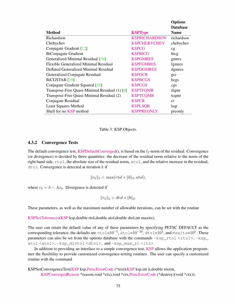
OptionsDatabase
Method KSPType NameRichardson KSPRICHARDSON richardsonChebychev KSPCHEBYCHEV chebychevConjugate Gradient [12] KSPCG cgBiConjugate Gradient KSPBICG bicgGeneralized Minimal Residual [16] KSPGMRES gmresFlexible Generalized Minimal Residual KSPFGMRES fgmresDeflated Generalized Minimal Residual KSPDGMRES dgmresGeneralized Conjugate Residual KSPGCR gcrBiCGSTAB [19] KSPBCGS bcgsConjugate Gradient Squared [18] KSPCGS cgsTranspose-Free Quasi-Minimal Residual (1) [8] KSPTFQMR tfqmrTranspose-Free Quasi-Minimal Residual (2) KSPTCQMR tcqmrConjugate Residual KSPCR crLeast Squares Method KSPLSQR lsqrShell for no KSP method KSPPREONLY preonly
Table 3: KSP Objects.
4.3.2 Convergence Tests
The default convergence test, KSPDefaultConverged(), is based on the l2-norm of the residual. Convergence(or divergence) is decided by three quantities: the decrease of the residual norm relative to the norm of theright hand side, rtol, the absolute size of the residual norm, atol, and the relative increase in the residual,dtol. Convergence is detected at iteration k if
‖rk‖2 < max(rtol ∗ ‖b‖2, atol),
where rk = b−Axk. Divergence is detected if
‖rk‖2 > dtol ∗ ‖b‖2.
These parameters, as well as the maximum number of allowable iterations, can be set with the routine
KSPSetTolerances(KSP ksp,double rtol,double atol,double dtol,int maxits);
The user can retain the default value of any of these parameters by specifying PETSC DEFAULT as thecorresponding tolerance; the defaults are rtol=10−5, atol=10−50, dtol=105, and maxits=105. Theseparameters can also be set from the options database with the commands -ksp_rtol <rtol>, -ksp_atol <atol>, -ksp_divtol <dtol>, and -ksp_max_it <its>.
In addition to providing an interface to a simple convergence test, KSP allows the application program-mer the flexibility to provide customized convergence-testing routines. The user can specify a customizedroutine with the command
KSPSetConvergenceTest(KSP ksp,PetscErrorCode (*test)(KSP ksp,int it,double rnorm,KSPConvergedReason *reason,void *ctx),void *ctx,PetscErrorCode (*destroy)(void *ctx));
75
The final routine argument, ctx, is an optional context for private data for the user-defined convergenceroutine, test. Other test routine arguments are the iteration number, it, and the residual’s l2 norm,rnorm. The routine for detecting convergence, test, should set reason to positive for convergence, 0 forno convergence, and negative for failure to converge. A list of possible KSPConvergedReason is given ininclude/petscksp.h. You can use KSPGetConvergedReason() after KSPSolve() to see why conver-gence/divergence was detected.
4.3.3 Convergence Monitoring
By default, the Krylov solvers run silently without displaying information about the iterations. The user canindicate that the norms of the residuals should be displayed by using -ksp_monitor within the optionsdatabase. To display the residual norms in a graphical window (running under X Windows), one should use -ksp_monitor_draw [x,y,w,h], where either all or none of the options must be specified. Applicationprogrammers can also provide their own routines to perform the monitoring by using the command
KSPMonitorSet(KSP ksp,PetscErrorCode (*mon)(KSP ksp,int it,double rnorm,void *ctx),void *ctx,PetscErrorCode (*mondestroy)(void**));
The final routine argument, ctx, is an optional context for private data for the user-defined monitoring rou-tine, mon. Other mon routine arguments are the iteration number (it) and the residual’s l2 norm (rnorm).A helpful routine within user-defined monitors is PetscObjectGetComm((PetscObject)ksp,MPI_Comm *comm), which returns in comm the MPI communicator for the KSP context. See section 1.3for more discussion of the use of MPI communicators within PETSc.
Several monitoring routines are supplied with PETSc, including
KSPMonitorDefault(KSP,int,double, void *);KSPMonitorSingularValue(KSP,int,double, void *);KSPMonitorTrueResidualNorm(KSP,int,double, void *);
The default monitor simply prints an estimate of the l2-norm of the residual at each iteration. The routineKSPMonitorSingularValue() is appropriate only for use with the conjugate gradient method or GMRES,since it prints estimates of the extreme singular values of the preconditioned operator at each iteration.Since KSPMonitorTrueResidualNorm() prints the true residual at each iteration by actually computing theresidual using the formula r = b−Ax, the routine is slow and should be used only for testing or convergencestudies, not for timing. These monitors may be accessed with the command line options -ksp_monitor,-ksp_monitor_singular_value, and -ksp_monitor_true_residual.
To employ the default graphical monitor, one should use the commands
PetscDrawLG lg;KSPMonitorLGCreate(char *display,char *title,int x,int y,int w,int h,PetscDrawLG *lg);KSPMonitorSet(KSP ksp,KSPMonitorLG,lg,0);
When no longer needed, the line graph should be destroyed with the command
KSPMonitorLGDestroy(PetscDrawLG *lg);
The user can change aspects of the graphs with the PetscDrawLG*() and PetscDrawAxis*() rou-tines. One can also access this functionality from the options database with the command -ksp_monitor_draw [x,y,w,h]. , where x, y, w, h are the optional location and size of the window.
One can cancel hardwired monitoring routines for KSP at runtime with -ksp_monitor_cancel.Unless the Krylov method converges so that the residual norm is small, say 10−10, many of the final
digits printed with the -ksp_monitor option are meaningless. Worse, they are different on different
76
machines; due to different round-off rules used by, say, the IBM RS6000 and the Sun Sparc. This makestesting between different machines difficult. The option -ksp_monitor_short causes PETSc to printfewer of the digits of the residual norm as it gets smaller; thus on most of the machines it will always printthe same numbers making cross system testing easier.
4.3.4 Understanding the Operator’s Spectrum
Since the convergence of Krylov subspace methods depends strongly on the spectrum (eigenvalues) of thepreconditioned operator, PETSc has specific routines for eigenvalue approximation via the Arnoldi or Lanc-zos iteration. First, before the linear solve one must call
KSPSetComputeEigenvalues(KSP ksp,PETSC TRUE);
Then after the KSP solve one calls
KSPComputeEigenvalues(KSP ksp, int n,double *realpart,double *complexpart,int *neig);
Here, n is the size of the two arrays and the eigenvalues are inserted into those two arrays. Neig is thenumber of eigenvalues computed; this number depends on the size of the Krylov space generated duringthe linear system solution, for GMRES it is never larger than the restart parameter. There is an additionalroutine
KSPComputeEigenvaluesExplicitly(KSP ksp, int n,double *realpart,double *complexpart);
that is useful only for very small problems. It explicitly computes the full representation of the precondi-tioned operator and calls LAPACK to compute its eigenvalues. It should be only used for matrices of sizeup to a couple hundred. The PetscDrawSP*() routines are very useful for drawing scatter plots of theeigenvalues.
The eigenvalues may also be computed and displayed graphically with the options data base com-mands -ksp_plot_eigenvalues and -ksp_plot_eigenvalues_explicitly. Or they canbe dumped to the screen in ASCII text via -ksp_compute_eigenvalues and -ksp_compute_eigenvalues_explicitly.
4.3.5 Other KSP Options
To obtain the solution vector and right hand side from a KSP context, one uses
KSPGetSolution(KSP ksp,Vec *x);KSPGetRhs(KSP ksp,Vec *rhs);
During the iterative process the solution may not yet have been calculated or it may be stored in a differentlocation. To access the approximate solution during the iterative process, one uses the command
KSPBuildSolution(KSP ksp,Vec w,Vec *v);
where the solution is returned in v. The user can optionally provide a vector in w as the location to storethe vector; however, if w is PETSC NULL, space allocated by PETSc in the KSP context is used. Oneshould not destroy this vector. For certain KSP methods, (e.g., GMRES), the construction of the solution isexpensive, while for many others it requires not even a vector copy.
Access to the residual is done in a similar way with the command
KSPBuildResidual(KSP ksp,Vec t,Vec w,Vec *v);
Again, for GMRES and certain other methods this is an expensive operation.
77
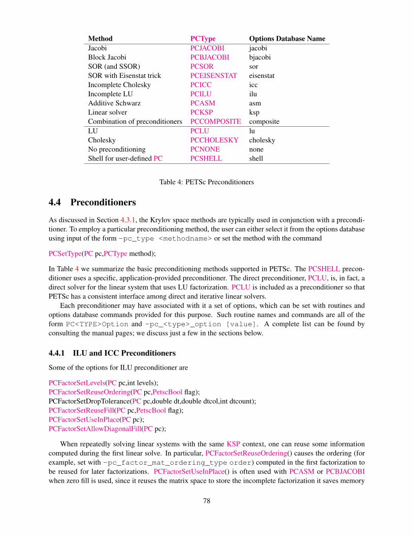
Method PCType Options Database NameJacobi PCJACOBI jacobiBlock Jacobi PCBJACOBI bjacobiSOR (and SSOR) PCSOR sorSOR with Eisenstat trick PCEISENSTAT eisenstatIncomplete Cholesky PCICC iccIncomplete LU PCILU iluAdditive Schwarz PCASM asmLinear solver PCKSP kspCombination of preconditioners PCCOMPOSITE compositeLU PCLU luCholesky PCCHOLESKY choleskyNo preconditioning PCNONE noneShell for user-defined PC PCSHELL shell
Table 4: PETSc Preconditioners
4.4 Preconditioners
As discussed in Section 4.3.1, the Krylov space methods are typically used in conjunction with a precondi-tioner. To employ a particular preconditioning method, the user can either select it from the options databaseusing input of the form -pc_type <methodname> or set the method with the command
PCSetType(PC pc,PCType method);
In Table 4 we summarize the basic preconditioning methods supported in PETSc. The PCSHELL precon-ditioner uses a specific, application-provided preconditioner. The direct preconditioner, PCLU, is, in fact, adirect solver for the linear system that uses LU factorization. PCLU is included as a preconditioner so thatPETSc has a consistent interface among direct and iterative linear solvers.
Each preconditioner may have associated with it a set of options, which can be set with routines andoptions database commands provided for this purpose. Such routine names and commands are all of theform PC<TYPE>Option and -pc_<type>_option [value]. A complete list can be found byconsulting the manual pages; we discuss just a few in the sections below.
4.4.1 ILU and ICC Preconditioners
Some of the options for ILU preconditioner are
PCFactorSetLevels(PC pc,int levels);PCFactorSetReuseOrdering(PC pc,PetscBool flag);PCFactorSetDropTolerance(PC pc,double dt,double dtcol,int dtcount);PCFactorSetReuseFill(PC pc,PetscBool flag);PCFactorSetUseInPlace(PC pc);PCFactorSetAllowDiagonalFill(PC pc);
When repeatedly solving linear systems with the same KSP context, one can reuse some informationcomputed during the first linear solve. In particular, PCFactorSetReuseOrdering() causes the ordering (forexample, set with -pc_factor_mat_ordering_type order) computed in the first factorization tobe reused for later factorizations. PCFactorSetUseInPlace() is often used with PCASM or PCBJACOBIwhen zero fill is used, since it reuses the matrix space to store the incomplete factorization it saves memory
78
and copying time. Note that in-place factorization is not appropriate with any ordering besides natural andcannot be used with the drop tolerance factorization. These options may be set in the database with
-pc_factor_levels <levels>-pc_factor_reuse_ordering-pc_factor_reuse_fill-pc_factor_in_place-pc_factor_nonzeros_along_diagonal-pc_factor_diagonal_fill
See Section 12.4.2 for information on preallocation of memory for anticipated fill during factorization.By alleviating the considerable overhead for dynamic memory allocation, such tuning can significantlyenhance performance.
PETSc supports incomplete factorization preconditioners for several matrix types for sequential matrix(for example MATSEQAIJ, MATSEQBAIJ, MATSEQSBAIJ).
4.4.2 SOR and SSOR Preconditioners
PETSc provides only a sequential SOR preconditioner that can only be used on sequential matrices or as thesubblock preconditioner when using block Jacobi or ASM preconditioning (see below).
The options for SOR preconditioning are
PCSORSetOmega(PC pc,double omega);PCSORSetIterations(PC pc,int its,int lits);PCSORSetSymmetric(PC pc,MatSORType type);
The first of these commands sets the relaxation factor for successive over (under) relaxation. The secondcommand sets the number of inner iterations its and local iterations lits (the number of smoothingsweeps on a process before doing a ghost point update from the other processes) to use between steps of theKrylov space method. The total number of SOR sweeps is given by its*lits. The third command setsthe kind of SOR sweep, where the argument type can be one of SOR_FORWARD_SWEEP, SOR_BACKWARD_SWEEP or SOR_SYMMETRIC_SWEEP, the default being SOR_FORWARD_SWEEP. Setting the typeto be SOR_SYMMETRIC_SWEEP produces the SSOR method. In addition, each process can locally andindependently perform the specified variant of SOR with the types SOR_LOCAL_FORWARD_SWEEP, SOR_LOCAL_BACKWARD_SWEEP, and SOR_LOCAL_SYMMETRIC_SWEEP. These variants can also be setwith the options -pc_sor_omega <omega>, -pc_sor_its <its>, -pc_sor_lits <lits>,-pc_sor_backward, -pc_sor_symmetric, -pc_sor_local_forward, -pc_sor_local_backward, and -pc_sor_local_symmetric.
The Eisenstat trick [5] for SSOR preconditioning can be employed with the method PCEISENSTAT(-pc_type eisenstat). By using both left and right preconditioning of the linear system, this vari-ant of SSOR requires about half of the floating-point operations for conventional SSOR. The option -pc_eisenstat_no_diagonal_scaling) (or the routine PCEisenstatNoDiagonalScaling()) turns offdiagonal scaling in conjunction with Eisenstat SSOR method, while the option -pc_eisenstat_omega<omega> (or the routine PCEisenstatSetOmega(PC pc,double omega)) sets the SSOR relaxation coeffi-cient, omega, as discussed above.
4.4.3 LU Factorization
The LU preconditioner provides several options. The first, given by the command
PCFactorSetUseInPlace(PC pc);
79
causes the factorization to be performed in-place and hence destroys the original matrix. The optionsdatabase variant of this command is -pc_factor_in_place. Another direct preconditioner optionis selecting the ordering of equations with the command
-pc_factor_mat_ordering_type <ordering>
The possible orderings are
• MATORDERINGNATURAL - Natural
• MATORDERINGND - Nested Dissection
• MATORDERING1WD - One-way Dissection
• MATORDERINGRCM - Reverse Cuthill-McKee
• MATORDERINGQMD - Quotient Minimum Degree
These orderings can also be set through the options database by specifying one of the following: -pc_factor_mat_ordering_type natural, or nd, or 1wd, or rcm, or qmd. In addition, see MatGe-tOrdering(), discussed in Section 15.2.
The sparse LU factorization provided in PETSc does not perform pivoting for numerical stability (sincethey are designed to preserve nonzero structure), thus occasionally a LU factorization will fail with azero pivot when, in fact, the matrix is non-singular. The option -pc_factor_nonzeros_along_diagonal <tol> will often help eliminate the zero pivot, by preprocessing the the column ordering toremove small values from the diagonal. Here, tol is an optional tolerance to decide if a value is nonzero;by default it is 1.e− 10.
In addition, Section 12.4.2 provides information on preallocation of memory for anticipated fill dur-ing factorization. Such tuning can significantly enhance performance, since it eliminates the considerableoverhead for dynamic memory allocation.
4.4.4 Block Jacobi and Overlapping Additive Schwarz Preconditioners
The block Jacobi and overlapping additive Schwarz methods in PETSc are supported in parallel; however,only the uniprocess version of the block Gauss-Seidel method is currently in place. By default, the PETScimplentations of these methods employ ILU(0) factorization on each individual block ( that is, the defaultsolver on each subblock is PCType=PCILU, KSPType=KSPPREONLY); the user can set alternative linearsolvers via the options -sub_ksp_type and -sub_pc_type. In fact, all of the KSP and PC optionscan be applied to the subproblems by inserting the prefix -sub_ at the beginning of the option name. Theseoptions database commands set the particular options for all of the blocks within the global problem. Inaddition, the routines
PCBJacobiGetSubKSP(PC pc,int *n local,int *first local,KSP **subksp);PCASMGetSubKSP(PC pc,int *n local,int *first local,KSP **subksp);
extract the KSP context for each local block. The argument n_local is the number of blocks on the callingprocess, and first_local indicates the global number of the first block on the process. The blocks arenumbered successively by processes from zero through gb − 1, where gb is the number of global blocks.The array of KSP contexts for the local blocks is given by subksp. This mechanism enables the user to setdifferent solvers for the various blocks. To set the appropriate data structures, the user must explicitly callKSPSetUp() before calling PCBJacobiGetSubKSP() or PCASMGetSubKSP(). For further details, see theexample ${PETSC_DIR}/src/ksp/ksp/examples/tutorials/ex7.c.
80
The block Jacobi, block Gauss-Seidel, and additive Schwarz preconditioners allow the user to set thenumber of blocks into which the problem is divided. The options database commands to set this value are-pc_bjacobi_blocks n and -pc_bgs_blocks n, and, within a program, the corresponding routinesare
PCBJacobiSetTotalBlocks(PC pc,int blocks,int *size);PCASMSetTotalSubdomains(PC pc,int n,IS *is);PCASMSetType(PC pc,PCASMType type);
The optional argument size, is an array indicating the size of each block. Currently, for certain parallelmatrix formats, only a single block per process is supported. However, the MATMPIAIJ and MATMPIBAIJformats support the use of general blocks as long as no blocks are shared among processes. The is argumentcontains the index sets that define the subdomains.
The object PCASMType is one of PC_ASM_BASIC, PC_ASM_INTERPOLATE, PC_ASM_RESTRICT, PC_ASM_NONE and may also be set with the options database -pc_asm_type [basic, interpolate,restrict, none]. The type PC_ASM_BASIC (or -pc_asm_type basic) corresponds to the stan-dard additive Schwarz method that uses the full restriction and interpolation operators. The type PC_ASM_RESTRICT (or -pc_asm_type restrict) uses a full restriction operator, but during the interpo-lation process ignores the off-process values. Similarly, PC_ASM_INTERPOLATE (or -pc_asm_typeinterpolate) uses a limited restriction process in conjunction with a full interpolation, while PC_ASM_NONE (or -pc_asm_type none) ignores off-process valies for both restriction and interpolation. TheASM types with limited restriction or interpolation were suggested by Xiao-Chuan Cai and Marcus Sarkis[3]. PC_ASM_RESTRICT is the PETSc default, as it saves substantial communication and for many prob-lems has the added benefit of requiring fewer iterations for convergence than the standard additive Schwarzmethod.
The user can also set the number of blocks and sizes on a per-process basis with the commands
PCBJacobiSetLocalBlocks(PC pc,int blocks,int *size);PCASMSetLocalSubdomains(PC pc,int N,IS *is);
For the ASM preconditioner one can use the following command to set the overlap to compute in con-structing the subdomains.
PCASMSetOverlap(PC pc,int overlap);
The overlap defaults to 1, so if one desires that no additional overlap be computed beyond what may havebeen set with a call to PCASMSetTotalSubdomains() or PCASMSetLocalSubdomains(), then overlapmust be set to be 0. In particular, if one does not explicitly set the subdomains in an application code,then all overlap would be computed internally by PETSc, and using an overlap of 0 would result in anASM variant that is equivalent to the block Jacobi preconditioner. Note that one can define initial indexsets is with any overlap via PCASMSetTotalSubdomains() or PCASMSetLocalSubdomains(); the routinePCASMSetOverlap() merely allows PETSc to extend that overlap further if desired.
4.4.5 Shell Preconditioners
The shell preconditioner simply uses an application-provided routine to implement the preconditioner. Toset this routine, one uses the command
PCShellSetApply(PC pc,PetscErrorCode (*apply)(PC,Vec,Vec));
Often a preconditioner needs access to an application-provided data structured. For this, one should use
PCShellSetContext(PC pc,void *ctx);
81
to set this data structure and
PCShellGetContext(PC pc,void **ctx);
to retrieve it in apply. The three routine arguments of apply() are the PC, the input vector, and theoutput vector, respectively.
For a preconditioner that requires some sort of “setup” before being used, that requires a new setupeverytime the operator is changed, one can provide a “setup” routine that is called everytime the operator ischanged (usually via KSPSetOperators()).
PCShellSetSetUp(PC pc,PetscErrorCode (*setup)(PC));
The argument to the “setup” routine is the same PC object which can be used to obtain the operators withPCGetOperators() and the application-provided data structure that was set with PCShellSetContext().
4.4.6 Combining Preconditioners
The PC type PCCOMPOSITE allows one to form new preconditioners by combining already defined pre-conditioners and solvers. Combining preconditioners usually requires some experimentation to find a com-bination of preconditioners that works better than any single method. It is a tricky business and is not rec-ommended until your application code is complete and running and you are trying to improve performance.In many cases using a single preconditioner is better than a combination; an exception is the multigrid/mul-tilevel preconditioners (solvers) that are always combinations of some sort, see Section 4.4.7.
Let B1 and B2 represent the application of two preconditioners of type type1 and type2. The pre-conditioner B = B1 +B2 can be obtained with
PCSetType(pc,PCCOMPOSITE);PCCompositeAddPC(pc,type1);PCCompositeAddPC(pc,type2);
Any number of preconditioners may added in this way.This way of combining preconditioners is called additive, since the actions of the preconditioners are
added together. This is the default behavior. An alternative can be set with the option
PCCompositeSetType(PC pc,PCCompositeType PC COMPOSITE MULTIPLICATIVE);
In this form the new residual is updated after the application of each preconditioner and the next precondi-tioner applied to the next residual. For example, with two composed preconditioners: B1 and B2; y = Bxis obtained from
y = B1x
w1 = x−Ayy = y +B2w1
Loosely, this corresponds to a Gauss-Siedel iteration, while additive corresponds to a Jacobi iteration.Under most circumstances the multiplicative form requires one-half the number of iterations as the
additive form; but the multiplicative form does require the application of A inside the preconditioner.In the multiplicative version, the calculation of the residual inside the preconditioner can be done in two
ways: using the original linear system matrix or using the matrix used to build the preconditioners B1, B2,etc. By default it uses the “preconditioner matrix”, to use the true matrix use the option
PCCompositeSetUseTrue(PC pc);
82
The individual preconditioners can be accessed (in order to set options) via
PCCompositeGetPC(PC pc,int count,PC *subpc);
For example, to set the first sub preconditioners to use ILU(1)
PC subpc;PCCompositeGetPC(pc,0,&subpc);PCFactorSetFill(subpc,1);
These various options can also be set via the options database. For example, -pc_type composite-pc_composite_pcs jacobi,ilu causes the composite preconditioner to be used with two precon-ditioners: Jacobi and ILU. The option -pc_composite_type multiplicative initiates the multi-plicative version of the algorithm, while -pc_composite_type additive the additive version. Usingthe true preconditioner is obtained with the option -pc_composite_true. One sets options for thesubpreconditioners with the extra prefix -sub_N_ where N is the number of the subpreconditioner. Forexample, -sub_0_pc_ifactor_fill 0.
PETSc also allows a preconditioner to be a complete linear solver. This is achieved with the PCKSPtype.
PCSetType(PC pc,PCKSP PCKSP);PCKSPGetKSP(pc,&ksp);/* set any KSP/PC options */
From the command line one can use 5 iterations of bi-CG-stab with ILU(0) preconditioning as the precondi-tioner with -pc_type ksp -ksp_pc_type ilu -ksp_ksp_max_it 5 -ksp_ksp_type bcgs.
By default the inner KSP preconditioner uses the outer preconditioner matrix as the matrix to be solvedin the linear system; to use the true matrix use the option
PCKSPSetUseTrue(PC pc);
or at the command line with -pc_ksp_true.Naturally one can use a KSP preconditioner inside a composite preconditioner. For example, -pc_
type composite -pc_composite_pcs ilu,ksp -sub_1_pc_type jacobi -sub_1_ksp_max_it 10 uses two preconditioners: ILU(0) and 10 iterations of GMRES with Jacobi preconditioning.Though it is not clear whether one would ever wish to do such a thing.
4.4.7 Multigrid Preconditioners
A large suite of routines is available for using multigrid as a preconditioner. In the PC framework theuser is required to provide the coarse grid solver, smoothers, restriction, and interpolation, as well as thecode to calculate residuals. The PC package allows all of that to be wrapped up into a PETSc compliantpreconditioner. We fully support both matrix-free and matrix-based multigrid solvers. See also Chapter7 for a higher level interface to the multigrid solvers for linear and nonlinear problems using the DMMGobject.
A multigrid preconditioner is created with the four commands
KSPCreate(MPI Comm comm,KSP *ksp);KSPGetPC(KSP ksp,PC *pc);PCSetType(PC pc,PCMG);PCMGSetLevels(pc,int levels,MPI Comm *comms);
A large number of parameters affect the multigrid behavior. The command
83
PCMGSetType(PC pc,PCMGType mode);
indicates which form of multigrid to apply [17].For standard V or W-cycle multigrids, one sets the mode to be PC_MG_MULTIPLICATIVE; for
the additive form (which in certain cases reduces to the BPX method, or additive multilevel Schwarz, ormultilevel diagonal scaling), one uses PC_MG_ADDITIVE as the mode. For a variant of full multigrid, onecan use PC_MG_FULL, and for the Kaskade algorithm PC_MG_KASKADE. For the multiplicative and fullmultigrid options, one can use a W-cycle by calling
PCMGSetCycleType(PC pc,PCMGCycleType ctype);
with a value of PC_MG_CYCLE_W for ctype. The commands above can also be set from the optionsdatabase. The option names are -pc_mg_type [multiplicative, additive, full, kaskade],and -pc_mg_cycle_type <ctype>.
The user can control the amount of pre- and postsmoothing by using either the options -pc_mg_smoothup m and -pc_mg_smoothdown n or the routines
PCMGSetNumberSmoothUp(PC pc,int m);PCMGSetNumberSmoothDown(PC pc,int n);
The multigrid routines, which determine the solvers and interpolation/restriction operators that are used,are mandatory. To set the coarse grid solver, one must call
PCMGGetCoarseSolve(PC pc,KSP *ksp);
and set the appropriate options in ksp. Similarly, the smoothers are set by calling
PCMGGetSmoother(PC pc,int level,KSP *ksp);
and setting the various options in ksp. To use a different pre- and postsmoother, one should call the fol-lowing routines instead.
PCMGGetSmootherUp(PC pc,int level,KSP *upksp);
and
PCMGGetSmootherDown(PC pc,int level,KSP *downksp);
Use
PCMGSetInterpolation(PC pc,int level,Mat P);
and
PCMGSetRestriction(PC pc,int level,Mat R);
to define the intergrid transfer operations. If only one of these is set, it’s transpose will be used for the other.It is possible for these interpolation operations to be matrix free (see Section 3.3), he or she should
make sure that these operations are defined for the (matrix-free) matrices passed in. Note that this system isarranged so that if the interpolation is the transpose of the restriction, you can pass the same mat argumentto both PCMGSetRestriction() and PCMGSetInterpolation().
On each level except the coarsest, one must also set the routine to compute the residual. The followingcommand suffices:
PCMGSetResidual(PC pc,int level,PetscErrorCode (*residual)(Mat,Vec,Vec,Vec),Mat mat);
84
The residual() function can be set to be PCMGDefaultResidual() if one’s operator is stored in a Mat format.In certain circumstances, where it is much cheaper to calculate the residual directly, rather than through theusual formula b−Ax, the user may wish to provide an alternative.
Finally, the user may provide three work vectors for each level (except on the finest, where only theresidual work vector is required). The work vectors are set with the commands
PCMGSetRhs(PC pc,int level,Vec b);PCMGSetX(PC pc,int level,Vec x);PCMGSetR(PC pc,int level,Vec r);
The PC references these vectors so you should call VecDestroy() when you are finished with them. If any ofthese vectors are not provided, the preconditioner will allocate them.
One can control the KSP and PC options used on the various levels (as well as the coarse grid) using theprefix mg_levels_ (mg_coarse_ for the coarse grid). For example,
-mg levels ksp type cg
will cause the CG method to be used as the Krylov method for each level. Or
-mg levels pc type ilu -mg levels pc factor levels 2
will cause the the ILU preconditioner to be used on each level with two levels of fill in the incompletefactorization.
4.5 Solving Block Matrices
Block matrices represent an important class of problems in numerical linear algebra and offer the possibilityof far more efficient iterative solvers than just treating the entire matrix as black box. In this section we areusing the common linear algebra definition of block matrices where matrices are divided in a small (two,three or so) number of very large blocks. Where the blocks arise naturally from the underlying physicsor discretization of the problem, for example, the velocity and pressure. Under a certain numbering ofunknowns the matrix can be written as
A00 A01 A02 A03
A10 A11 A12 A13
A20 A21 A22 A23
A30 A31 A32 A33
.Where each Aij is an entire block. In a parallel computer the matrices are not stored explicitly this wayhowever, each process will own some of the rows of A0∗, A1∗ etc. On a process the blocks may be storedone block followed by another
A0000 A0001 A0002 ... A0100 A0102 ...A0010 A0011 A0012 ... A0110 A0112 ...A0020 A0021 A0022 ... A0120 A0122 ......
A1000 A1001 A1002 ... A1100 A1102 ...A1010 A1011 A1012 ... A1110 A1112 ......
85
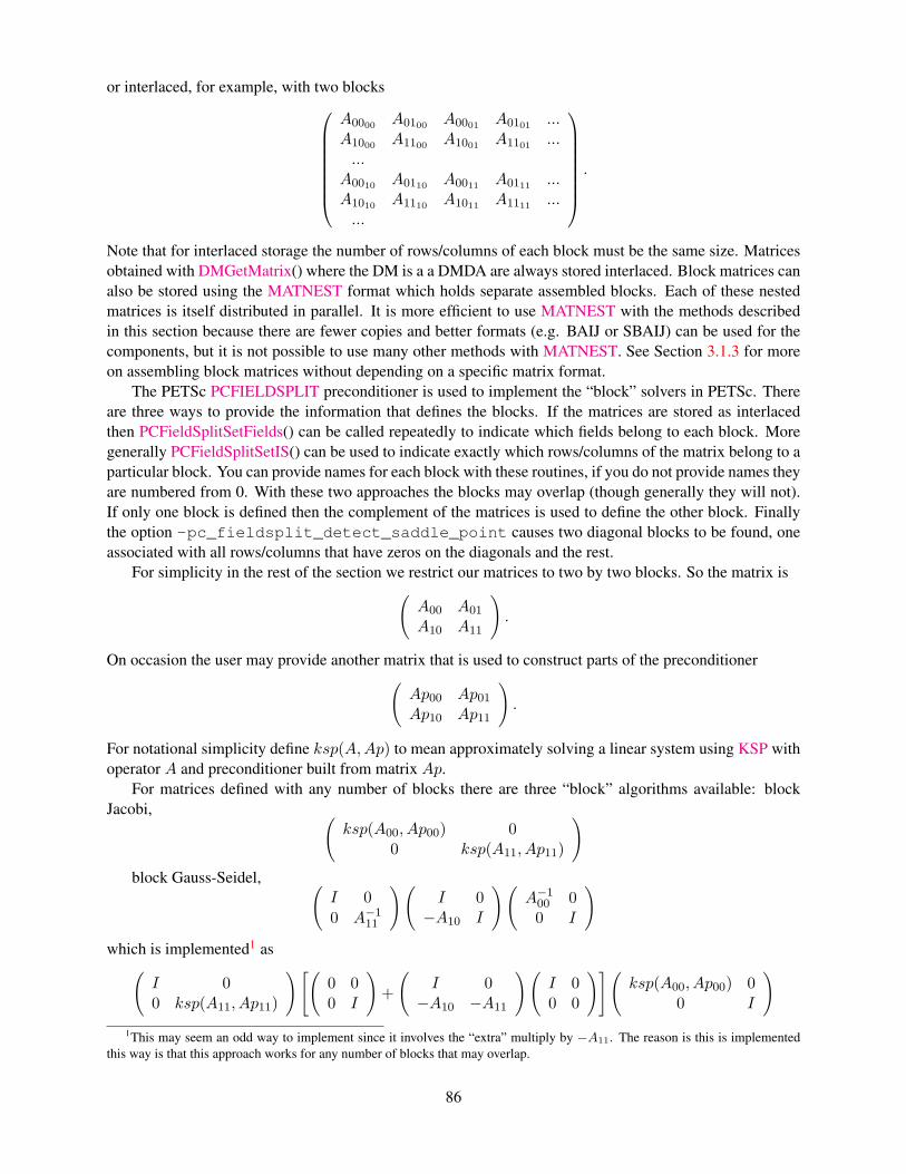
or interlaced, for example, with two blocks
A0000 A0100 A0001 A0101 ...A1000 A1100 A1001 A1101 ......
A0010 A0110 A0011 A0111 ...A1010 A1110 A1011 A1111 ......
.
Note that for interlaced storage the number of rows/columns of each block must be the same size. Matricesobtained with DMGetMatrix() where the DM is a a DMDA are always stored interlaced. Block matrices canalso be stored using the MATNEST format which holds separate assembled blocks. Each of these nestedmatrices is itself distributed in parallel. It is more efficient to use MATNEST with the methods describedin this section because there are fewer copies and better formats (e.g. BAIJ or SBAIJ) can be used for thecomponents, but it is not possible to use many other methods with MATNEST. See Section 3.1.3 for moreon assembling block matrices without depending on a specific matrix format.
The PETSc PCFIELDSPLIT preconditioner is used to implement the “block” solvers in PETSc. Thereare three ways to provide the information that defines the blocks. If the matrices are stored as interlacedthen PCFieldSplitSetFields() can be called repeatedly to indicate which fields belong to each block. Moregenerally PCFieldSplitSetIS() can be used to indicate exactly which rows/columns of the matrix belong to aparticular block. You can provide names for each block with these routines, if you do not provide names theyare numbered from 0. With these two approaches the blocks may overlap (though generally they will not).If only one block is defined then the complement of the matrices is used to define the other block. Finallythe option -pc_fieldsplit_detect_saddle_point causes two diagonal blocks to be found, oneassociated with all rows/columns that have zeros on the diagonals and the rest.
For simplicity in the rest of the section we restrict our matrices to two by two blocks. So the matrix is(A00 A01
A10 A11
).
On occasion the user may provide another matrix that is used to construct parts of the preconditioner(Ap00 Ap01
Ap10 Ap11
).
For notational simplicity define ksp(A,Ap) to mean approximately solving a linear system using KSP withoperator A and preconditioner built from matrix Ap.
For matrices defined with any number of blocks there are three “block” algorithms available: blockJacobi, (
ksp(A00, Ap00) 00 ksp(A11, Ap11)
)block Gauss-Seidel, (
I 00 A−1
11
)(I 0−A10 I
)(A−1
00 00 I
)which is implemented1 as(
I 00 ksp(A11, Ap11)
)[(0 00 I
)+
(I 0−A10 −A11
)(I 00 0
)](ksp(A00, Ap00) 0
0 I
)1This may seem an odd way to implement since it involves the “extra” multiply by −A11. The reason is this is implemented
this way is that this approach works for any number of blocks that may overlap.
86
and symmetric block Gauss-Seidel(A−1
00 00 I
)(I −A01
0 I
)(A00 00 A−1
11
)(I 0−A10 I
)(A−1
00 00 I
).
These can be access with -pc_fieldsplit_type <additive,multiplicative,symmetric_multiplicative> or the function PCFieldSplitSetType(). The option prefixes for the internal KSPs aregiven by -fieldsplit_name_.
For two by two blocks only there are another family of solvers, based on Schur complements. Theinverse of the Schur complement factorization is[(
I 0A10A
−100 I
)(A00 00 S
)(I A−1
00 A01
0 I
)]−1
(I A−1
00 A01
0 I
)−1(A−1
00 00 S−1
)(I 0
A10A−100 I
)−1
(I −A−1
00 A01
0 I
)(A−1
00 00 S−1
)(I 0
−A10A−100 I
)
(A−1
00 00 I
)(I −A01
0 I
)(A00 00 S−1
)(I 0−A10 I
)(A−1
00 00 I
).
The preconditioner is accessed with -pc_fieldsplit_type schur and is implemented as(ksp(A00, Ap00) 0
0 I
)(I −A01
0 I
)(I 00 ksp(S, Sp)
)(I 0
−A10ksp(A00, Ap00) I
).
Where S = A11 −A10ksp(A00, Ap00)A01 is the approximate Schur complement. By default Sp is Ap11.There are several variants of the Schur complement preconditioner obtained by dropping some of
the terms, these can be obtained with -pc_fieldsplit_schur_factorization_type <diag,lower,upper,full> or NOTE WE NEED TO ADD A FUNCTIONAL INTERFACE. Note that thediag form uses the preconditioner(
ksp(A00, Ap00) 00 −ksp(S, Sp)
)since the Schur complement for saddle point problems is negative definite. IS THIS ALWAYS TRUE,SHOULD THERE BE A FLAG TO SET THE SIGN?
You can use the PCLSC preconditioner for the Schur complement with -pc_fieldsplit_typeschur -fieldsplit_1_pc_type lsc. This uses for the preconditioner to S the operator
ksp(A10A01, A10A01)A10A00A01ksp(A10A01, A10A01)
which, of course, introduces two additional inner solves for each application of the Schur complement. Theoptions prefix for this inner KSP is -fieldsplit_1_lsc_. Instead of constructing the matrix A10A01
the user can provide their own matrix. This is done by attaching the matrix/matrices to the Sp matrix theyprovide with
PetscObjectCompose((PetscObject)Sp,”LSC L”,(PetscObject)L);PetscObjectCompose((PetscObject)Sp,”LSC Lp”,(PetscObject)Lp);
87
4.6 Solving Singular Systems
Sometimes one is required to solver linear systems that are singular. That is systems with the matrix has anull space. For example, the discretization of the Laplacian operator with Neumann boundary conditions asa null space of the constant functions. PETSc has tools to help solve these systems.
First, one must know what the null space is and store it using an orthonormal basis in an array of PETScVecs. (The constant functions can be handled separately, since they are such a common case). Create aMatNullSpace object with the command
MatNullSpaceCreate(MPI Comm,PetscBool hasconstants,int dim,Vec *basis,MatNullSpace *nsp);
Here dim is the number of vectors in basis and hasconstants indicates if the null space contains theconstant functions. (If the null space contains the constant functions you do not need to include it in thebasis vectors you provide).
One then tells the KSP object you are using what the null space is with the call
KSPSetNullSpace(KSP ksp,MatNullSpace nsp);
The PETSc solvers will now handle the null space during the solution process.But if one chooses a direct solver (or an incomplete factorization) it may still detect a zero pivot.
You can run with the additional options -pc_factor_shift_nonzero <dampingfactor> or -pc_factor_shift_nonzero <dampingfactor> to prevent the zero pivot. A good choice for thedamping factor is 1.e-10.
4.7 Using PETSc to interface with external linear solvers
PETSc interfaces to several external linear solvers (see Acknowledgments). To use these solvers, one needsto:
1. Run ./configure with the additional options --download-packagename. For eg: --download-superlu_dist --download-parmetis (SuperLU DIST needs ParMetis) or --download-mumps --download-scalapack --download-blacs (MUMPS requires ScaLAPACK andBLACS).
2. Build the PETSc libraries.
3. Use the runtime option: -ksp_type preonly -pc_type <pctype> -pc_factor_mat_solver_package <packagename>. For eg: -ksp_type preonly -pc_type lu -pc_factor_mat_solver_package superlu_dist.
88
MatType PCType MatSolverPackage Package(-pc_factor_mat_solver_package)
seqaij lu MATSOLVERESSL esslseqaij lu MATSOLVERLUSOL lusolseqaij lu MATSOLVERMATLAB matlabaij lu MATSOLVERMUMPS mumpsaij choleskysbaij choleskympidense lu MATSOLVERPLAPACK plapackmpidense choleskyaij lu MATSOLVERSPOOLES spoolessbaij choleskyseqaij lu MATSOLVERSUPERLU superluaij lu MATSOLVERSUPERLU DIST superlu_distseqaij lu MATSOLVERUMFPACK umfpack
Table 5: Options for External Solvers
The default and available input options for each external software can be found by specifying -help (or-h) at runtime.
As an alternative to using runtime flags to employ these external packages, procedural calls are providedfor some packages. For example, following procedural calls are equivalent to runtime options -ksp_typepreonly -pc_type lu -pc_factor_mat_solver_package mumps -mat_mumps_icntl_7 2:
KSPSetType(ksp,KSPPREONLY);KSPGetPC(ksp,&pc);PCSetType(pc,PCLU);PCFactorSetMatSolverPackage(pc,MATSOLVERMUMPS);PCFactorGetMatrix(pc,&F);icntl=7; ival = 2;MatMumpsSetIcntl(F,icntl,ival);
One can also create matrices with the appropriate capabilities by calling MatCreate() followed by Mat-SetType() specifying the desired matrix type from Table 5. These matrix types inherit capabilities fromtheir PETSc matrix parents: seqaij, mpiaij, etc. As a result, the preallocation routines MatSeqAIJSetPre-allocation(), MatMPIAIJSetPreallocation(), etc. and any other type specific routines of the base class aresupported. One can also call MatConvert() inplace to convert the matrix to and from its base class with-out performing an expensive data copy. MatConvert() cannot be called on matrices that have already beenfactored.
In Table 5, the base class aij refers to the fact that inheritance is based on MATSEQAIJ when con-structed with a single process communicator, and from MATMPIAIJ otherwise. The same holds for baij andsbaij. For codes that are intended to be run as both a single process or with multiple processes, dependingon the mpiexec command, it is recommended that both sets of preallocation routines are called for thesecommunicator morphing types. The call for the incorrect type will simply be ignored without any harm ormessage.
89

90
Chapter 5
SNES: Nonlinear Solvers
The solution of large-scale nonlinear problems pervades many facets of computational science and demandsrobust and flexible solution strategies. The SNES library of PETSc provides a powerful suite of data-structure-neutral numerical routines for such problems. Built on top of the linear solvers and data structuresdiscussed in preceding chapters, SNES enables the user to easily customize the nonlinear solvers accordingto the application at hand. Also, the SNES interface is identical for the uniprocess and parallel cases; theonly difference in the parallel version is that each process typically forms only its local contribution tovarious matrices and vectors.
The SNES class includes methods for solving systems of nonlinear equations of the form
F (x) = 0, (5.1)
where F : <n → <n. Newton-like methods provide the core of the package, including both line search andtrust region techniques, which are discussed further in Section 5.2. Following the PETSc design philosophy,the interfaces to the various solvers are all virtually identical. In addition, the SNES software is completelyflexible, so that the user can at runtime change any facet of the solution process.
The general form of the n-dimensional Newton’s method for solving (5.1) is
xk+1 = xk − [F ′(xk)]−1F (xk), k = 0, 1, . . . , (5.2)
where x0 is an initial approximation to the solution and F ′(xk), the Jacobian, is nonsingular at each itera-tion. In practice, the Newton iteration (5.2) is implemented by the following two steps:
1. (Approximately) solve F ′(xk)∆xk = −F (xk). (5.3)
2. Update xk+1 = xk + ∆xk. (5.4)
5.1 Basic SNES Usage
In the simplest usage of the nonlinear solvers, the user must merely provide a C, C++, or Fortran routine toevaluate the nonlinear function of Equation (5.1). The corresponding Jacobian matrix can be approximatedwith finite differences. For codes that are typically more efficient and accurate, the user can provide aroutine to compute the Jacobian; details regarding these application-provided routines are discussed below.To provide an overview of the use of the nonlinear solvers, we first introduce a complete and simple examplein Figure 14, corresponding to ${PETSC_DIR}/src/snes/examples/tutorials/ex1.c.
static char help[] = "Newton’s method for a two-variable system, sequential.\n\n";
91
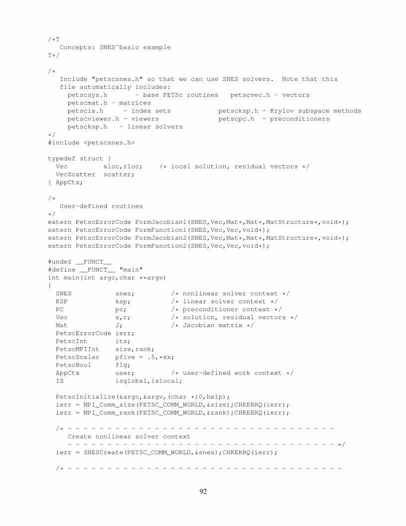
/*TConcepts: SNESˆbasic example
T*/
/*Include "petscsnes.h" so that we can use SNES solvers. Note that thisfile automatically includes:
petscsys.h - base PETSc routines petscvec.h - vectorspetscmat.h - matricespetscis.h - index sets petscksp.h - Krylov subspace methodspetscviewer.h - viewers petscpc.h - preconditionerspetscksp.h - linear solvers
*/#include <petscsnes.h>
typedef struct {Vec xloc,rloc; /* local solution, residual vectors */VecScatter scatter;
} AppCtx;
/*User-defined routines
*/extern PetscErrorCode FormJacobian1(SNES,Vec,Mat*,Mat*,MatStructure*,void*);extern PetscErrorCode FormFunction1(SNES,Vec,Vec,void*);extern PetscErrorCode FormJacobian2(SNES,Vec,Mat*,Mat*,MatStructure*,void*);extern PetscErrorCode FormFunction2(SNES,Vec,Vec,void*);
#undef __FUNCT__#define __FUNCT__ "main"int main(int argc,char **argv){
SNES snes; /* nonlinear solver context */KSP ksp; /* linear solver context */PC pc; /* preconditioner context */Vec x,r; /* solution, residual vectors */Mat J; /* Jacobian matrix */PetscErrorCode ierr;PetscInt its;PetscMPIInt size,rank;PetscScalar pfive = .5,*xx;PetscBool flg;AppCtx user; /* user-defined work context */IS isglobal,islocal;
PetscInitialize(&argc,&argv,(char *)0,help);ierr = MPI_Comm_size(PETSC_COMM_WORLD,&size);CHKERRQ(ierr);ierr = MPI_Comm_rank(PETSC_COMM_WORLD,&rank);CHKERRQ(ierr);
/* - - - - - - - - - - - - - - - - - - - - - - - - - - - - - - - - - -Create nonlinear solver context- - - - - - - - - - - - - - - - - - - - - - - - - - - - - - - - - - */
ierr = SNESCreate(PETSC_COMM_WORLD,&snes);CHKERRQ(ierr);
/* - - - - - - - - - - - - - - - - - - - - - - - - - - - - - - - - - - -
92
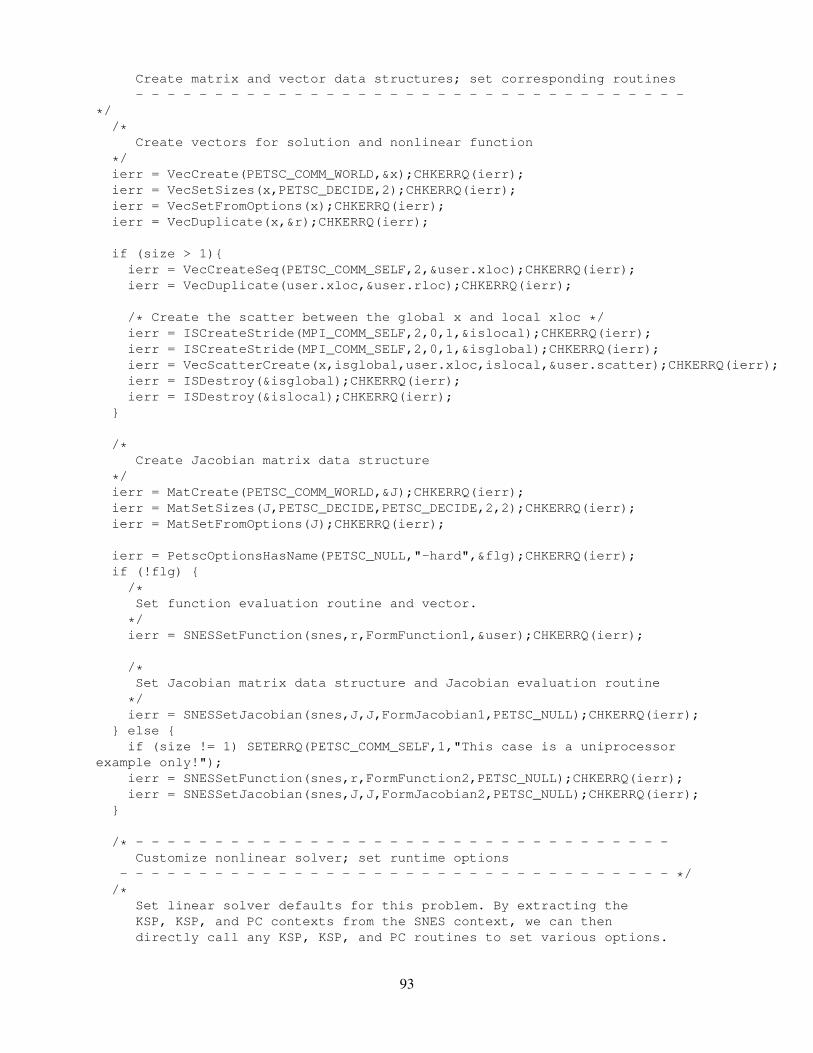
Create matrix and vector data structures; set corresponding routines- - - - - - - - - - - - - - - - - - - - - - - - - - - - - - - - - - -
*//*
Create vectors for solution and nonlinear function
*/ierr = VecCreate(PETSC_COMM_WORLD,&x);CHKERRQ(ierr);ierr = VecSetSizes(x,PETSC_DECIDE,2);CHKERRQ(ierr);ierr = VecSetFromOptions(x);CHKERRQ(ierr);ierr = VecDuplicate(x,&r);CHKERRQ(ierr);
if (size > 1){ierr = VecCreateSeq(PETSC_COMM_SELF,2,&user.xloc);CHKERRQ(ierr);ierr = VecDuplicate(user.xloc,&user.rloc);CHKERRQ(ierr);
/* Create the scatter between the global x and local xloc */ierr = ISCreateStride(MPI_COMM_SELF,2,0,1,&islocal);CHKERRQ(ierr);ierr = ISCreateStride(MPI_COMM_SELF,2,0,1,&isglobal);CHKERRQ(ierr);ierr = VecScatterCreate(x,isglobal,user.xloc,islocal,&user.scatter);CHKERRQ(ierr);ierr = ISDestroy(&isglobal);CHKERRQ(ierr);ierr = ISDestroy(&islocal);CHKERRQ(ierr);
}
/*Create Jacobian matrix data structure
*/ierr = MatCreate(PETSC_COMM_WORLD,&J);CHKERRQ(ierr);ierr = MatSetSizes(J,PETSC_DECIDE,PETSC_DECIDE,2,2);CHKERRQ(ierr);ierr = MatSetFromOptions(J);CHKERRQ(ierr);
ierr = PetscOptionsHasName(PETSC_NULL,"-hard",&flg);CHKERRQ(ierr);if (!flg) {
/*Set function evaluation routine and vector.
*/ierr = SNESSetFunction(snes,r,FormFunction1,&user);CHKERRQ(ierr);
/*Set Jacobian matrix data structure and Jacobian evaluation routine
*/ierr = SNESSetJacobian(snes,J,J,FormJacobian1,PETSC_NULL);CHKERRQ(ierr);
} else {if (size != 1) SETERRQ(PETSC_COMM_SELF,1,"This case is a uniprocessor
example only!");ierr = SNESSetFunction(snes,r,FormFunction2,PETSC_NULL);CHKERRQ(ierr);ierr = SNESSetJacobian(snes,J,J,FormJacobian2,PETSC_NULL);CHKERRQ(ierr);
}
/* - - - - - - - - - - - - - - - - - - - - - - - - - - - - - - - - - -Customize nonlinear solver; set runtime options
- - - - - - - - - - - - - - - - - - - - - - - - - - - - - - - - - - - *//*
Set linear solver defaults for this problem. By extracting theKSP, KSP, and PC contexts from the SNES context, we can thendirectly call any KSP, KSP, and PC routines to set various options.
93
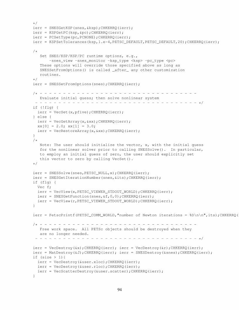
*/ierr = SNESGetKSP(snes,&ksp);CHKERRQ(ierr);ierr = KSPGetPC(ksp,&pc);CHKERRQ(ierr);ierr = PCSetType(pc,PCNONE);CHKERRQ(ierr);ierr = KSPSetTolerances(ksp,1.e-4,PETSC_DEFAULT,PETSC_DEFAULT,20);CHKERRQ(ierr);
/*Set SNES/KSP/KSP/PC runtime options, e.g.,
-snes_view -snes_monitor -ksp_type <ksp> -pc_type <pc>These options will override those specified above as long asSNESSetFromOptions() is called _after_ any other customizationroutines.
*/ierr = SNESSetFromOptions(snes);CHKERRQ(ierr);
/* - - - - - - - - - - - - - - - - - - - - - - - - - - - - - - - - - -Evaluate initial guess; then solve nonlinear system
- - - - - - - - - - - - - - - - - - - - - - - - - - - - - - - - - - - */if (!flg) {
ierr = VecSet(x,pfive);CHKERRQ(ierr);} else {
ierr = VecGetArray(x,&xx);CHKERRQ(ierr);xx[0] = 2.0; xx[1] = 3.0;ierr = VecRestoreArray(x,&xx);CHKERRQ(ierr);
}/*
Note: The user should initialize the vector, x, with the initial guessfor the nonlinear solver prior to calling SNESSolve(). In particular,to employ an initial guess of zero, the user should explicitly setthis vector to zero by calling VecSet().
*/
ierr = SNESSolve(snes,PETSC_NULL,x);CHKERRQ(ierr);ierr = SNESGetIterationNumber(snes,&its);CHKERRQ(ierr);if (flg) {
Vec f;ierr = VecView(x,PETSC_VIEWER_STDOUT_WORLD);CHKERRQ(ierr);ierr = SNESGetFunction(snes,&f,0,0);CHKERRQ(ierr);ierr = VecView(r,PETSC_VIEWER_STDOUT_WORLD);CHKERRQ(ierr);
}
ierr = PetscPrintf(PETSC_COMM_WORLD,"number of Newton iterations = %D\n\n",its);CHKERRQ(ierr);
/* - - - - - - - - - - - - - - - - - - - - - - - - - - - - - - - - - -Free work space. All PETSc objects should be destroyed when theyare no longer needed.
- - - - - - - - - - - - - - - - - - - - - - - - - - - - - - - - - - - */
ierr = VecDestroy(&x);CHKERRQ(ierr); ierr = VecDestroy(&r);CHKERRQ(ierr);ierr = MatDestroy(&J);CHKERRQ(ierr); ierr = SNESDestroy(&snes);CHKERRQ(ierr);if (size > 1){
ierr = VecDestroy(&user.xloc);CHKERRQ(ierr);ierr = VecDestroy(&user.rloc);CHKERRQ(ierr);ierr = VecScatterDestroy(&user.scatter);CHKERRQ(ierr);
}
94

ierr = PetscFinalize();return 0;
}/* ------------------------------------------------------------------- */#undef __FUNCT__#define __FUNCT__ "FormFunction1"/*
FormFunction1 - Evaluates nonlinear function, F(x).
Input Parameters:. snes - the SNES context. x - input vector. ctx - optional user-defined context
Output Parameter:. f - function vector
*/PetscErrorCode FormFunction1(SNES snes,Vec x,Vec f,void *ctx){
PetscErrorCode ierr;PetscScalar *xx,*ff;AppCtx *user = (AppCtx*)ctx;Vec xloc=user->xloc,floc=user->rloc;VecScatter scatter=user->scatter;MPI_Comm comm;PetscMPIInt size,rank;PetscInt rstart,rend;
ierr = PetscObjectGetComm((PetscObject)snes,&comm);CHKERRQ(ierr);ierr = MPI_Comm_size(comm,&size);CHKERRQ(ierr);ierr = MPI_Comm_rank(comm,&rank);CHKERRQ(ierr);if (size > 1){
/*This is a ridiculous case for testing intermidiate steps from sequential
code development to parallel implementation.(1) scatter x into a sequetial vector;(2) each process evaluates all values of floc;(3) scatter floc back to the parallel f.
*/ierr = VecScatterBegin(scatter,x,xloc,INSERT_VALUES,SCATTER_FORWARD);CHKERRQ(ierr);ierr = VecScatterEnd(scatter,x,xloc,INSERT_VALUES,SCATTER_FORWARD);CHKERRQ(ierr);
ierr = VecGetOwnershipRange(f,&rstart,&rend);CHKERRQ(ierr);ierr = VecGetArray(xloc,&xx);CHKERRQ(ierr);ierr = VecGetArray(floc,&ff);CHKERRQ(ierr);ff[0] = xx[0]*xx[0] + xx[0]*xx[1] - 3.0;ff[1] = xx[0]*xx[1] + xx[1]*xx[1] - 6.0;ierr = VecRestoreArray(floc,&ff);CHKERRQ(ierr);ierr = VecRestoreArray(xloc,&xx);CHKERRQ(ierr);
ierr = VecScatterBegin(scatter,floc,f,INSERT_VALUES,SCATTER_REVERSE);CHKERRQ(ierr);ierr = VecScatterEnd(scatter,floc,f,INSERT_VALUES,SCATTER_REVERSE);CHKERRQ(ierr);
} else {/*Get pointers to vector data.
95
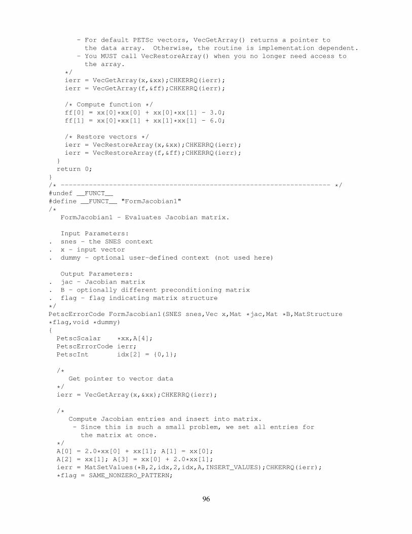
- For default PETSc vectors, VecGetArray() returns a pointer tothe data array. Otherwise, the routine is implementation dependent.
- You MUST call VecRestoreArray() when you no longer need access tothe array.
*/ierr = VecGetArray(x,&xx);CHKERRQ(ierr);ierr = VecGetArray(f,&ff);CHKERRQ(ierr);
/* Compute function */ff[0] = xx[0]*xx[0] + xx[0]*xx[1] - 3.0;ff[1] = xx[0]*xx[1] + xx[1]*xx[1] - 6.0;
/* Restore vectors */ierr = VecRestoreArray(x,&xx);CHKERRQ(ierr);ierr = VecRestoreArray(f,&ff);CHKERRQ(ierr);
}return 0;
}/* ------------------------------------------------------------------- */#undef __FUNCT__#define __FUNCT__ "FormJacobian1"/*
FormJacobian1 - Evaluates Jacobian matrix.
Input Parameters:. snes - the SNES context. x - input vector. dummy - optional user-defined context (not used here)
Output Parameters:. jac - Jacobian matrix. B - optionally different preconditioning matrix. flag - flag indicating matrix structure
*/PetscErrorCode FormJacobian1(SNES snes,Vec x,Mat *jac,Mat *B,MatStructure
*flag,void *dummy){
PetscScalar *xx,A[4];PetscErrorCode ierr;PetscInt idx[2] = {0,1};
/*Get pointer to vector data
*/ierr = VecGetArray(x,&xx);CHKERRQ(ierr);
/*Compute Jacobian entries and insert into matrix.- Since this is such a small problem, we set all entries for
the matrix at once.
*/A[0] = 2.0*xx[0] + xx[1]; A[1] = xx[0];A[2] = xx[1]; A[3] = xx[0] + 2.0*xx[1];ierr = MatSetValues(*B,2,idx,2,idx,A,INSERT_VALUES);CHKERRQ(ierr);
*flag = SAME_NONZERO_PATTERN;
96
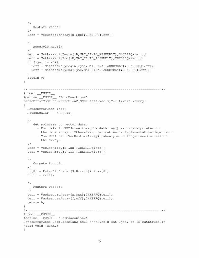
/*Restore vector
*/ierr = VecRestoreArray(x,&xx);CHKERRQ(ierr);
/*Assemble matrix
*/ierr = MatAssemblyBegin(*B,MAT_FINAL_ASSEMBLY);CHKERRQ(ierr);ierr = MatAssemblyEnd(*B,MAT_FINAL_ASSEMBLY);CHKERRQ(ierr);if (*jac != *B){ierr = MatAssemblyBegin(*jac,MAT_FINAL_ASSEMBLY);CHKERRQ(ierr);ierr = MatAssemblyEnd(*jac,MAT_FINAL_ASSEMBLY);CHKERRQ(ierr);
}return 0;
}
/* ------------------------------------------------------------------- */#undef __FUNCT__#define __FUNCT__ "FormFunction2"PetscErrorCode FormFunction2(SNES snes,Vec x,Vec f,void *dummy){
PetscErrorCode ierr;PetscScalar *xx,*ff;
/*Get pointers to vector data.
- For default PETSc vectors, VecGetArray() returns a pointer tothe data array. Otherwise, the routine is implementation dependent.
- You MUST call VecRestoreArray() when you no longer need access tothe array.
*/ierr = VecGetArray(x,&xx);CHKERRQ(ierr);ierr = VecGetArray(f,&ff);CHKERRQ(ierr);
/*Compute function
*/ff[0] = PetscSinScalar(3.0*xx[0]) + xx[0];ff[1] = xx[1];
/*Restore vectors
*/ierr = VecRestoreArray(x,&xx);CHKERRQ(ierr);ierr = VecRestoreArray(f,&ff);CHKERRQ(ierr);return 0;
}/* ------------------------------------------------------------------- */#undef __FUNCT__#define __FUNCT__ "FormJacobian2"PetscErrorCode FormJacobian2(SNES snes,Vec x,Mat *jac,Mat *B,MatStructure
*flag,void *dummy){
97
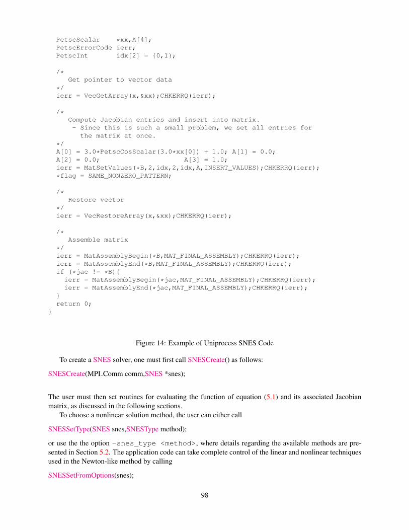
PetscScalar *xx,A[4];PetscErrorCode ierr;PetscInt idx[2] = {0,1};
/*Get pointer to vector data
*/ierr = VecGetArray(x,&xx);CHKERRQ(ierr);
/*Compute Jacobian entries and insert into matrix.- Since this is such a small problem, we set all entries for
the matrix at once.
*/A[0] = 3.0*PetscCosScalar(3.0*xx[0]) + 1.0; A[1] = 0.0;A[2] = 0.0; A[3] = 1.0;ierr = MatSetValues(*B,2,idx,2,idx,A,INSERT_VALUES);CHKERRQ(ierr);
*flag = SAME_NONZERO_PATTERN;
/*Restore vector
*/ierr = VecRestoreArray(x,&xx);CHKERRQ(ierr);
/*Assemble matrix
*/ierr = MatAssemblyBegin(*B,MAT_FINAL_ASSEMBLY);CHKERRQ(ierr);ierr = MatAssemblyEnd(*B,MAT_FINAL_ASSEMBLY);CHKERRQ(ierr);if (*jac != *B){ierr = MatAssemblyBegin(*jac,MAT_FINAL_ASSEMBLY);CHKERRQ(ierr);ierr = MatAssemblyEnd(*jac,MAT_FINAL_ASSEMBLY);CHKERRQ(ierr);
}return 0;
}
Figure 14: Example of Uniprocess SNES Code
To create a SNES solver, one must first call SNESCreate() as follows:
SNESCreate(MPI Comm comm,SNES *snes);
The user must then set routines for evaluating the function of equation (5.1) and its associated Jacobianmatrix, as discussed in the following sections.
To choose a nonlinear solution method, the user can either call
SNESSetType(SNES snes,SNESType method);
or use the the option -snes_type <method>, where details regarding the available methods are pre-sented in Section 5.2. The application code can take complete control of the linear and nonlinear techniquesused in the Newton-like method by calling
SNESSetFromOptions(snes);
98
This routine provides an interface to the PETSc options database, so that at runtime the user can selecta particular nonlinear solver, set various parameters and customized routines (e.g., specialized line searchvariants), prescribe the convergence tolerance, and set monitoring routines. With this routine the user canalso control all linear solver options in the KSP, and PC modules, as discussed in Chapter 4.
After having set these routines and options, the user solves the problem by calling
SNESSolve(SNES snes,Vec b,Vec x);
where x indicates the solution vector. The user should initialize this vector to the initial guess for thenonlinear solver prior to calling SNESSolve(). In particular, to employ an initial guess of zero, the usershould explicitly set this vector to zero by calling VecSet(). Finally, after solving the nonlinear system (orseveral systems), the user should destroy the SNES context with
SNESDestroy(SNES *snes);
5.1.1 Nonlinear Function Evaluation
When solving a system of nonlinear equations, the user must provide a vector, f, for storing the function ofEquation (5.1), as well as a routine that evaluates this function at the vector x. This information should beset with the command
SNESSetFunction(SNES snes,Vec f,PetscErrorCode (*FormFunction)(SNES snes,Vec x,Vec f,void *ctx),void *ctx);
The argument ctx is an optional user-defined context, which can store any private, application-specificdata required by the function evaluation routine; PETSC NULL should be used if such information is notneeded. In C and C++, a user-defined context is merely a structure in which various objects can be stashed; inFortran a user context can be an integer array that contains both parameters and pointers to PETSc objects.${PETSC_DIR}/src/snes/examples/tutorials/ex5.c and ${PETSC_DIR}/src/snes/examples/tutorials/ex5f.F give examples of user-defined application contexts in C and Fortran,respectively.
5.1.2 Jacobian Evaluation
The user must also specify a routine to form some approximation of the Jacobian matrix, A, at the currentiterate, x, as is typically done with
SNESSetJacobian(SNES snes,Mat A,Mat B,PetscErrorCode (*FormJacobian)(SNES snes,Vec x,Mat *A,Mat *B,MatStructure *flag,void *ctx),void *ctx);
The arguments of the routine FormJacobian() are the current iterate, x; the Jacobian matrix, A; thepreconditioner matrix, B (which is usually the same as A); a flag indicating information about the precon-ditioner matrix structure; and an optional user-defined Jacobian context, ctx, for application-specific data.The options for flag are identical to those for the flag of KSPSetOperators(), discussed in Section 4.1.Note that the SNES solvers are all data-structure neutral, so the full range of PETSc matrix formats (includ-ing “matrix-free” methods) can be used. Chapter 3 discusses information regarding available matrix formatsand options, while Section 5.5 focuses on matrix-free methods in SNES. We briefly touch on a few detailsof matrix usage that are particularly important for efficient use of the nonlinear solvers.
A common usage paradigm is to assemble the problem Jacobian in the preconditioner storage B, ratherthan A. In the case where they are identical, as in many simulations, this makes no difference. However, itallows us to check the analytic Jacobian we construct in FormJacobian() by passing the -snes_mf_operator flag. This causes PETSc to approximate the Jacobian using finite differencing of the function
99
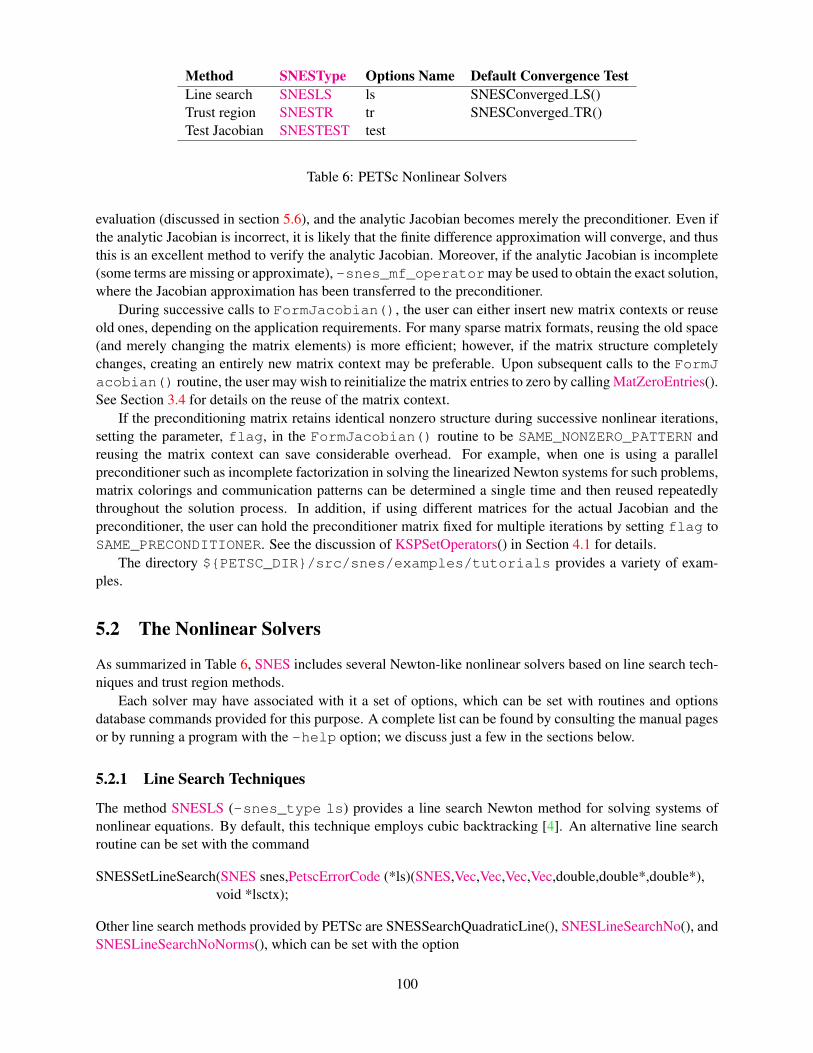
Method SNESType Options Name Default Convergence TestLine search SNESLS ls SNESConverged LS()Trust region SNESTR tr SNESConverged TR()Test Jacobian SNESTEST test
Table 6: PETSc Nonlinear Solvers
evaluation (discussed in section 5.6), and the analytic Jacobian becomes merely the preconditioner. Even ifthe analytic Jacobian is incorrect, it is likely that the finite difference approximation will converge, and thusthis is an excellent method to verify the analytic Jacobian. Moreover, if the analytic Jacobian is incomplete(some terms are missing or approximate), -snes_mf_operatormay be used to obtain the exact solution,where the Jacobian approximation has been transferred to the preconditioner.
During successive calls to FormJacobian(), the user can either insert new matrix contexts or reuseold ones, depending on the application requirements. For many sparse matrix formats, reusing the old space(and merely changing the matrix elements) is more efficient; however, if the matrix structure completelychanges, creating an entirely new matrix context may be preferable. Upon subsequent calls to the FormJacobian() routine, the user may wish to reinitialize the matrix entries to zero by calling MatZeroEntries().See Section 3.4 for details on the reuse of the matrix context.
If the preconditioning matrix retains identical nonzero structure during successive nonlinear iterations,setting the parameter, flag, in the FormJacobian() routine to be SAME_NONZERO_PATTERN andreusing the matrix context can save considerable overhead. For example, when one is using a parallelpreconditioner such as incomplete factorization in solving the linearized Newton systems for such problems,matrix colorings and communication patterns can be determined a single time and then reused repeatedlythroughout the solution process. In addition, if using different matrices for the actual Jacobian and thepreconditioner, the user can hold the preconditioner matrix fixed for multiple iterations by setting flag toSAME_PRECONDITIONER. See the discussion of KSPSetOperators() in Section 4.1 for details.
The directory ${PETSC_DIR}/src/snes/examples/tutorials provides a variety of exam-ples.
5.2 The Nonlinear Solvers
As summarized in Table 6, SNES includes several Newton-like nonlinear solvers based on line search tech-niques and trust region methods.
Each solver may have associated with it a set of options, which can be set with routines and optionsdatabase commands provided for this purpose. A complete list can be found by consulting the manual pagesor by running a program with the -help option; we discuss just a few in the sections below.
5.2.1 Line Search Techniques
The method SNESLS (-snes_type ls) provides a line search Newton method for solving systems ofnonlinear equations. By default, this technique employs cubic backtracking [4]. An alternative line searchroutine can be set with the command
SNESSetLineSearch(SNES snes,PetscErrorCode (*ls)(SNES,Vec,Vec,Vec,Vec,double,double*,double*),void *lsctx);
Other line search methods provided by PETSc are SNESSearchQuadraticLine(), SNESLineSearchNo(), andSNESLineSearchNoNorms(), which can be set with the option
100
-snes_ls [cubic, quadratic, basic, basicnonorms]
The line search routines involve several parameters, which are set to defaults that are reasonable for manyapplications. The user can override the defaults by using the options -snes_ls_alpha <alpha>,-snes_ls_maxstep <max>, and -snes_ls_steptol <tol>.
5.2.2 Trust Region Methods
The trust region method in SNES for solving systems of nonlinear equations, SNESTR (-snes_typetr), is taken from the MINPACK project [13]. Several parameters can be set to control the variation of thetrust region size during the solution process. In particular, the user can control the initial trust region radius,computed by
∆ = ∆0‖F0‖2,by setting ∆0 via the option -snes_tr_delta0 <delta0>.
5.3 General Options
This section discusses options and routines that apply to all SNES solvers and problem classes. In particular,we focus on convergence tests, monitoring routines, and tools for checking derivative computations.
5.3.1 Convergence Tests
Convergence of the nonlinear solvers can be detected in a variety of ways; the user can even specify acustomized test, as discussed below. The default convergence routines for the various nonlinear solverswithin SNES are listed in Table 6; see the corresponding manual pages for detailed descriptions. Eachof these convergence tests involves several parameters, which are set by default to values that should bereasonable for a wide range of problems. The user can customize the parameters to the problem at hand byusing some of the following routines and options.
One method of convergence testing is to declare convergence when the norm of the change in the solutionbetween successive iterations is less than some tolerance, stol. Convergence can also be determined basedon the norm of the function Such a test can use either the absolute size of the norm, atol, or its relativedecrease, rtol, from an initial guess. The following routine sets these parameters, which are used in manyof the default SNES convergence tests:
SNESSetTolerances(SNES snes,double atol,double rtol,double stol,int its,int fcts);
This routine also sets the maximum numbers of allowable nonlinear iterations, its, and function evalu-ations, fcts. The corresponding options database commands for setting these parameters are -snes_atol <atol>, -snes_rtol <rtol>, -snes_stol <stol>, -snes_max_it <its>, and-snes_max_funcs <fcts>. A related routine is SNESGetTolerances().
Convergence tests for trust regions methods often use an additional parameter that indicates the min-imium allowable trust region radius. The user can set this parameter with the option -snes_trtol<trtol> or with the routine
SNESSetTrustRegionTolerance(SNES snes,double trtol);
Users can set their own customized convergence tests in SNES by using the command
SNESSetConvergenceTest(SNES snes,PetscErrorCode (*test)(SNES snes,int it,double xnorm,double gnorm,double f,SNESConvergedReason reason,void *cctx),void *cctx,PetscErrorCode (*destroy)(void *cctx));
101
The final argument of the convergence test routine, cctx, denotes an optional user-defined context forprivate data. When solving systems of nonlinear equations, the arguments xnorm, gnorm, and f are thecurrent iterate norm, current step norm, and function norm, respectively. SNESConvergedReason shouldbe set positive for convergence and negative for divergence. See include/petscsnes.h for a list ofvalues for SNESConvergedReason.
5.3.2 Convergence Monitoring
By default the SNES solvers run silently without displaying information about the iterations. The user caninitiate monitoring with the command
SNESMonitorSet(SNES snes,PetscErrorCode (*mon)(SNES,int its,double norm,void* mctx),void *mctx,PetscErrorCode (*monitordestroy)(void**));
The routine, mon, indicates a user-defined monitoring routine, where its and mctx respectively denote theiteration number and an optional user-defined context for private data for the monitor routine. The argumentnorm is the function norm.
The routine set by SNESMonitorSet() is called once after every successful step computation withinthe nonlinear solver. Hence, the user can employ this routine for any application-specific computations thatshould be done after the solution update. The option -snes_monitor activates the default SNES monitorroutine, SNESMonitorDefault(), while -snes_monitor_draw draws a simple line graph of the residualnorm’s convergence.
Once can cancel hardwired monitoring routines for SNES at runtime with -snes_monitor_cancel.
As the Newton method converges so that the residual norm is small, say 10−10, many of the finaldigits printed with the -snes_monitor option are meaningless. Worse, they are different on differentmachines; due to different round-off rules used by, say, the IBM RS6000 and the Sun Sparc. This makestesting between different machines difficult. The option -snes_monitor_short causes PETSc to printfewer of the digits of the residual norm as it gets smaller; thus on most of the machines it will always printthe same numbers making cross process testing easier.
The routines
SNESGetSolution(SNES snes,Vec *x);SNESGetFunction(SNES snes,Vec *r,void *ctx,
int(**func)(SNES,Vec,Vec,void*));
return the solution vector and function vector from a SNES context. These routines are useful, for instance,if the convergence test requires some property of the solution or function other than those passed with routinearguments.
5.3.3 Checking Accuracy of Derivatives
Since hand-coding routines for Jacobian matrix evaluation can be error prone, SNES provides easy-to-usesupport for checking these matrices against finite difference versions. In the simplest form of comparison,users can employ the option -snes_type test to compare the matrices at several points. Althoughnot exhaustive, this test will generally catch obvious problems. One can compare the elements of the twomatrices by using the option -snes_test_display , which causes the two matrices to be printed tothe screen.
Another means for verifying the correctness of a code for Jacobian computation is running the problemwith either the finite difference or matrix-free variant, -snes_fd or -snes_mf. see Section 5.6 or Section5.5). If a problem converges well with these matrix approximations but not with a user-provided routine, theproblem probably lies with the hand-coded matrix.
102
5.4 Inexact Newton-like Methods
Since exact solution of the linear Newton systems within (5.2) at each iteration can be costly, modifica-tions are often introduced that significantly reduce these expenses and yet retain the rapid convergence ofNewton’s method. Inexact or truncated Newton techniques approximately solve the linear systems usingan iterative scheme. In comparison with using direct methods for solving the Newton systems, iterativemethods have the virtue of requiring little space for matrix storage and potentially saving significant com-putational work. Within the class of inexact Newton methods, of particular interest are Newton-Krylovmethods, where the subsidiary iterative technique for solving the Newton system is chosen from the class ofKrylov subspace projection methods. Note that at runtime the user can set any of the linear solver optionsdiscussed in Chapter 4, such as -ksp_type <ksp_method> and -pc_type <pc_method>, to setthe Krylov subspace and preconditioner methods.
Two levels of iterations occur for the inexact techniques, where during each global or outer Newtoniteration a sequence of subsidiary inner iterations of a linear solver is performed. Appropriate control of theaccuracy to which the subsidiary iterative method solves the Newton system at each global iteration is crit-ical, since these inner iterations determine the asymptotic convergence rate for inexact Newton techniques.While the Newton systems must be solved well enough to retain fast local convergence of the Newton’siterates, use of excessive inner iterations, particularly when ‖xk−x∗‖ is large, is neither necessary nor eco-nomical. Thus, the number of required inner iterations typically increases as the Newton process progresses,so that the truncated iterates approach the true Newton iterates.
A sequence of nonnegative numbers {ηk} can be used to indicate the variable convergence criterion.In this case, when solving a system of nonlinear equations, the update step of the Newton process remainsunchanged, and direct solution of the linear system is replaced by iteration on the system until the residuals
r(i)k = F ′(xk)∆xk + F (xk)
satisfy
‖r(i)k ‖
‖F (xk)‖≤ ηk ≤ η < 1.
Here x0 is an initial approximation of the solution, and ‖ · ‖ denotes an arbitrary norm in <n .By default a constant relative convergence tolerance is used for solving the subsidiary linear systems
within the Newton-like methods of SNES. When solving a system of nonlinear equations, one can insteademploy the techniques of Eisenstat and Walker [6] to compute ηk at each step of the nonlinear solver byusing the option -snes_ksp_ew_conv . In addition, by adding one’s own KSP convergence test (seeSection 4.3.2), one can easily create one’s own, problem-dependent, inner convergence tests.
5.5 Matrix-Free Methods
The SNES class fully supports matrix-free methods. The matrices specified in the Jacobian evaluation rou-tine need not be conventional matrices; instead, they can point to the data required to implement a particularmatrix-free method. The matrix-free variant is allowed only when the linear systems are solved by an it-erative method in combination with no preconditioning (PCNONE or -pc_type none), a user-providedpreconditioner matrix, or a user-provided preconditioner shell (PCSHELL, discussed in Section 4.4); thatis, obviously matrix-free methods cannot be used if a direct solver is to be employed.
The user can create a matrix-free context for use within SNES with the routine
MatCreateSNESMF(SNES snes,Mat *mat);
103
This routine creates the data structures needed for the matrix-vector products that arise within Krylov spaceiterative methods [2] by employing the matrix type MATSHELL, discussed in Section 3.3. The defaultSNES matrix-free approximations can also be invoked with the command -snes_mf. Or, one can retainthe user-provided Jacobian preconditioner, but replace the user-provided Jacobian matrix with the defaultmatrix free variant with the option -snes_mf_operator.
See also
MatCreateMFFD(Vec x, Mat *mat);
for users who need a matrix-free matrix but are not using SNES.The user can set one parameter to control the Jacobian-vector product approximation with the command
MatMFFDSetFunctionError(Mat mat,double rerror);
The parameter rerror should be set to the square root of the relative error in the function evaluations, erel;the default is 10−8, which assumes that the functions are evaluated to full double precision accuracy. Thisparameter can also be set from the options database with
-snes mf err <err>
In addition, SNES provides a way to register new routines to compute the differencing parameter (h);see the manual page for MatMFFDSetType() and MatMFFDRegisterDynamic). We currently provide twodefault routines accessible via
-snes mf type <default or wp>
For the default approach there is one “tuning” parameter, set with
MatMFFDDSSetUmin(Mat mat,PetscReal umin);
This parameter, umin (or umin), is a bit involved; its default is 10−6 . The Jacobian-vector product isapproximated via the formula
F ′(u)a ≈ F (u+ h ∗ a)− F (u)h
where h is computed via
h = erel ∗ uTa/||a||22 if|u′a| > umin ∗ ||a||1= erel ∗ umin ∗ sign(uTa) ∗ ||a||1/||a||22 otherwise.
This approach is taken from Brown and Saad [2]. The parameter can also be set from the options databasewith
-snes mf umin <umin>
The second approach, taken from Walker and Pernice, [15], computes h via
h =√
1 + ||u||erel
||a||
This has no tunable parameters, but note that inside the nonlinear solve for the entire linear iterative processu does not change hence
√1 + ||u|| need be computed only once. This information may be set with the
options
MatMFFDWPSetComputeNormU(Mat mat,PetscBool );
104
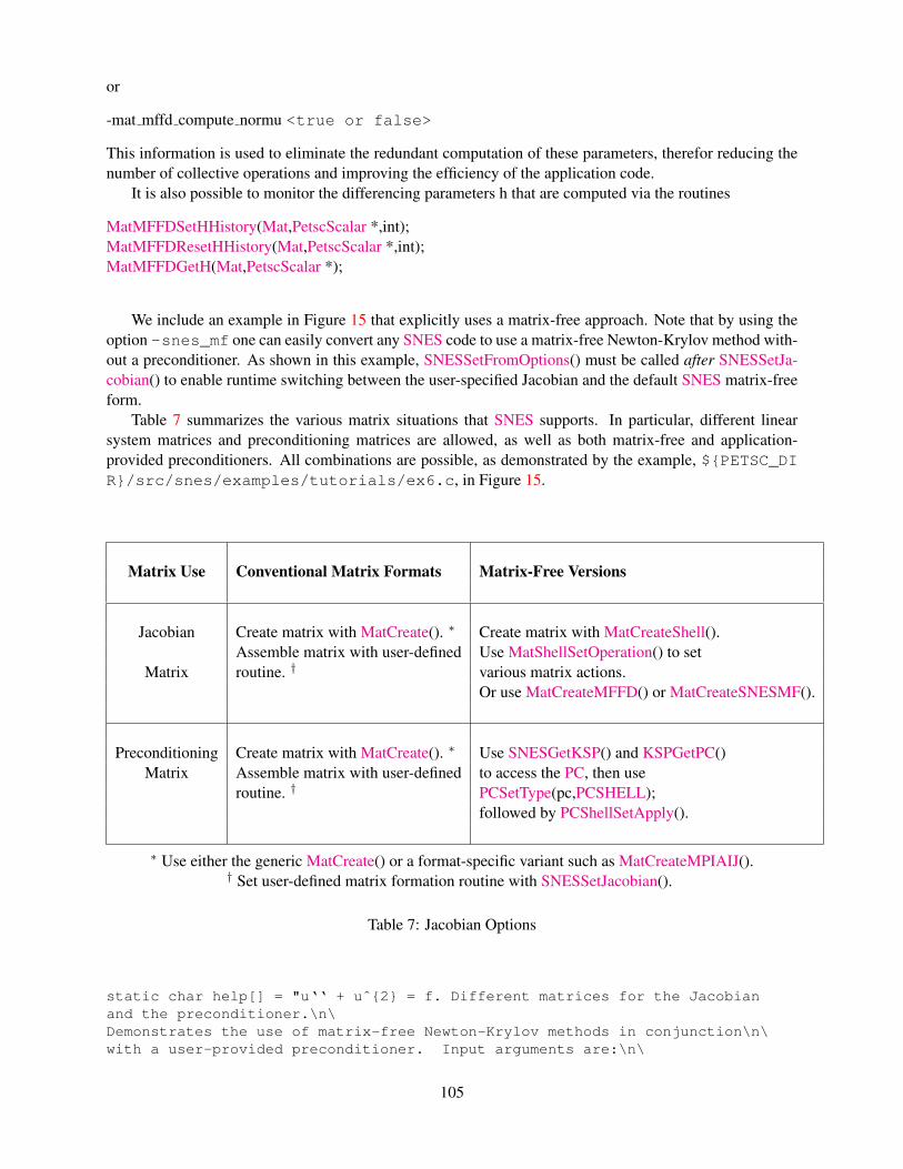
or
-mat mffd compute normu <true or false>
This information is used to eliminate the redundant computation of these parameters, therefor reducing thenumber of collective operations and improving the efficiency of the application code.
It is also possible to monitor the differencing parameters h that are computed via the routines
MatMFFDSetHHistory(Mat,PetscScalar *,int);MatMFFDResetHHistory(Mat,PetscScalar *,int);MatMFFDGetH(Mat,PetscScalar *);
We include an example in Figure 15 that explicitly uses a matrix-free approach. Note that by using theoption -snes_mf one can easily convert any SNES code to use a matrix-free Newton-Krylov method with-out a preconditioner. As shown in this example, SNESSetFromOptions() must be called after SNESSetJa-cobian() to enable runtime switching between the user-specified Jacobian and the default SNES matrix-freeform.
Table 7 summarizes the various matrix situations that SNES supports. In particular, different linearsystem matrices and preconditioning matrices are allowed, as well as both matrix-free and application-provided preconditioners. All combinations are possible, as demonstrated by the example, ${PETSC_DIR}/src/snes/examples/tutorials/ex6.c, in Figure 15.
Matrix Use Conventional Matrix Formats Matrix-Free Versions
Jacobian Create matrix with MatCreate(). ∗ Create matrix with MatCreateShell().Assemble matrix with user-defined Use MatShellSetOperation() to set
Matrix routine. † various matrix actions.Or use MatCreateMFFD() or MatCreateSNESMF().
Preconditioning Create matrix with MatCreate(). ∗ Use SNESGetKSP() and KSPGetPC()Matrix Assemble matrix with user-defined to access the PC, then use
routine. † PCSetType(pc,PCSHELL);followed by PCShellSetApply().
∗ Use either the generic MatCreate() or a format-specific variant such as MatCreateMPIAIJ().† Set user-defined matrix formation routine with SNESSetJacobian().
Table 7: Jacobian Options
static char help[] = "u‘‘ + uˆ{2} = f. Different matrices for the Jacobianand the preconditioner.\n\Demonstrates the use of matrix-free Newton-Krylov methods in conjunction\n\with a user-provided preconditioner. Input arguments are:\n\
105
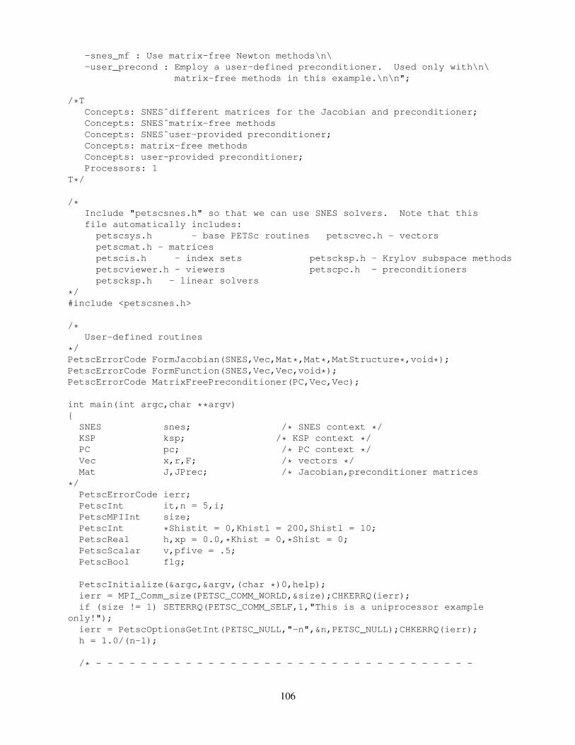
-snes_mf : Use matrix-free Newton methods\n\-user_precond : Employ a user-defined preconditioner. Used only with\n\
matrix-free methods in this example.\n\n";
/*TConcepts: SNESˆdifferent matrices for the Jacobian and preconditioner;Concepts: SNESˆmatrix-free methodsConcepts: SNESˆuser-provided preconditioner;Concepts: matrix-free methodsConcepts: user-provided preconditioner;Processors: 1
T*/
/*Include "petscsnes.h" so that we can use SNES solvers. Note that thisfile automatically includes:
petscsys.h - base PETSc routines petscvec.h - vectorspetscmat.h - matricespetscis.h - index sets petscksp.h - Krylov subspace methodspetscviewer.h - viewers petscpc.h - preconditionerspetscksp.h - linear solvers
*/#include <petscsnes.h>
/*User-defined routines
*/PetscErrorCode FormJacobian(SNES,Vec,Mat*,Mat*,MatStructure*,void*);PetscErrorCode FormFunction(SNES,Vec,Vec,void*);PetscErrorCode MatrixFreePreconditioner(PC,Vec,Vec);
int main(int argc,char **argv){
SNES snes; /* SNES context */KSP ksp; /* KSP context */PC pc; /* PC context */Vec x,r,F; /* vectors */Mat J,JPrec; /* Jacobian,preconditioner matrices
*/PetscErrorCode ierr;PetscInt it,n = 5,i;PetscMPIInt size;PetscInt *Shistit = 0,Khistl = 200,Shistl = 10;PetscReal h,xp = 0.0,*Khist = 0,*Shist = 0;PetscScalar v,pfive = .5;PetscBool flg;
PetscInitialize(&argc,&argv,(char *)0,help);ierr = MPI_Comm_size(PETSC_COMM_WORLD,&size);CHKERRQ(ierr);if (size != 1) SETERRQ(PETSC_COMM_SELF,1,"This is a uniprocessor example
only!");ierr = PetscOptionsGetInt(PETSC_NULL,"-n",&n,PETSC_NULL);CHKERRQ(ierr);h = 1.0/(n-1);
/* - - - - - - - - - - - - - - - - - - - - - - - - - - - - - - - - - -
106
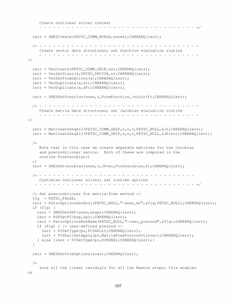
Create nonlinear solver context- - - - - - - - - - - - - - - - - - - - - - - - - - - - - - - - - - */
ierr = SNESCreate(PETSC_COMM_WORLD,&snes);CHKERRQ(ierr);
/* - - - - - - - - - - - - - - - - - - - - - - - - - - - - - - - - - - -Create vector data structures; set function evaluation routine- - - - - - - - - - - - - - - - - - - - - - - - - - - - - - - - - - -
*/
ierr = VecCreate(PETSC_COMM_SELF,&x);CHKERRQ(ierr);ierr = VecSetSizes(x,PETSC_DECIDE,n);CHKERRQ(ierr);ierr = VecSetFromOptions(x);CHKERRQ(ierr);ierr = VecDuplicate(x,&r);CHKERRQ(ierr);ierr = VecDuplicate(x,&F);CHKERRQ(ierr);
ierr = SNESSetFunction(snes,r,FormFunction,(void*)F);CHKERRQ(ierr);
/* - - - - - - - - - - - - - - - - - - - - - - - - - - - - - - - - - - -Create matrix data structures; set Jacobian evaluation routine- - - - - - - - - - - - - - - - - - - - - - - - - - - - - - - - - - -
*/
ierr = MatCreateSeqAIJ(PETSC_COMM_SELF,n,n,3,PETSC_NULL,&J);CHKERRQ(ierr);ierr = MatCreateSeqAIJ(PETSC_COMM_SELF,n,n,1,PETSC_NULL,&JPrec);CHKERRQ(ierr);
/*Note that in this case we create separate matrices for the Jacobianand preconditioner matrix. Both of these are computed in theroutine FormJacobian()
*/ierr = SNESSetJacobian(snes,J,JPrec,FormJacobian,0);CHKERRQ(ierr);
/* - - - - - - - - - - - - - - - - - - - - - - - - - - - - - - - - - -Customize nonlinear solver; set runtime options
- - - - - - - - - - - - - - - - - - - - - - - - - - - - - - - - - - - */
/* Set preconditioner for matrix-free method */flg = PETSC_FALSE;ierr = PetscOptionsGetBool(PETSC_NULL,"-snes_mf",&flg,PETSC_NULL);CHKERRQ(ierr);if (flg) {
ierr = SNESGetKSP(snes,&ksp);CHKERRQ(ierr);ierr = KSPGetPC(ksp,&pc);CHKERRQ(ierr);ierr = PetscOptionsHasName(PETSC_NULL,"-user_precond",&flg);CHKERRQ(ierr);if (flg) { /* user-defined precond */
ierr = PCSetType(pc,PCSHELL);CHKERRQ(ierr);ierr = PCShellSetApply(pc,MatrixFreePreconditioner);CHKERRQ(ierr);
} else {ierr = PCSetType(pc,PCNONE);CHKERRQ(ierr);}}
ierr = SNESSetFromOptions(snes);CHKERRQ(ierr);
/*Save all the linear residuals for all the Newton steps; this enables
us
107
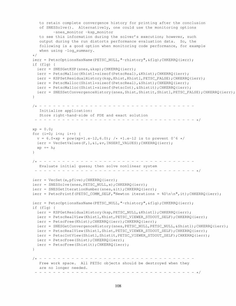
to retain complete convergence history for printing after the conclusionof SNESSolve(). Alternatively, one could use the monitoring options
-snes_monitor -ksp_monitorto see this information during the solver’s execution; however, suchoutput during the run distorts performance evaluation data. So, thefollowing is a good option when monitoring code performance, for examplewhen using -log_summary.
*/ierr = PetscOptionsHasName(PETSC_NULL,"-rhistory",&flg);CHKERRQ(ierr);if (flg) {
ierr = SNESGetKSP(snes,&ksp);CHKERRQ(ierr);ierr = PetscMalloc(Khistl*sizeof(PetscReal),&Khist);CHKERRQ(ierr);ierr = KSPSetResidualHistory(ksp,Khist,Khistl,PETSC_FALSE);CHKERRQ(ierr);ierr = PetscMalloc(Shistl*sizeof(PetscReal),&Shist);CHKERRQ(ierr);ierr = PetscMalloc(Shistl*sizeof(PetscInt),&Shistit);CHKERRQ(ierr);ierr = SNESSetConvergenceHistory(snes,Shist,Shistit,Shistl,PETSC_FALSE);CHKERRQ(ierr);
}
/* - - - - - - - - - - - - - - - - - - - - - - - - - - - - - - - - - -Initialize application:Store right-hand-side of PDE and exact solution
- - - - - - - - - - - - - - - - - - - - - - - - - - - - - - - - - - - */
xp = 0.0;for (i=0; i<n; i++) {
v = 6.0*xp + pow(xp+1.e-12,6.0); /* +1.e-12 is to prevent 0ˆ6 */ierr = VecSetValues(F,1,&i,&v,INSERT_VALUES);CHKERRQ(ierr);xp += h;
}
/* - - - - - - - - - - - - - - - - - - - - - - - - - - - - - - - - - -Evaluate initial guess; then solve nonlinear system
- - - - - - - - - - - - - - - - - - - - - - - - - - - - - - - - - - - */
ierr = VecSet(x,pfive);CHKERRQ(ierr);ierr = SNESSolve(snes,PETSC_NULL,x);CHKERRQ(ierr);ierr = SNESGetIterationNumber(snes,&it);CHKERRQ(ierr);ierr = PetscPrintf(PETSC_COMM_SELF,"Newton iterations = %D\n\n",it);CHKERRQ(ierr);
ierr = PetscOptionsHasName(PETSC_NULL,"-rhistory",&flg);CHKERRQ(ierr);if (flg) {
ierr = KSPGetResidualHistory(ksp,PETSC_NULL,&Khistl);CHKERRQ(ierr);ierr = PetscRealView(Khistl,Khist,PETSC_VIEWER_STDOUT_SELF);CHKERRQ(ierr);ierr = PetscFree(Khist);CHKERRQ(ierr);CHKERRQ(ierr);ierr = SNESGetConvergenceHistory(snes,PETSC_NULL,PETSC_NULL,&Shistl);CHKERRQ(ierr);ierr = PetscRealView(Shistl,Shist,PETSC_VIEWER_STDOUT_SELF);CHKERRQ(ierr);ierr = PetscIntView(Shistl,Shistit,PETSC_VIEWER_STDOUT_SELF);CHKERRQ(ierr);ierr = PetscFree(Shist);CHKERRQ(ierr);ierr = PetscFree(Shistit);CHKERRQ(ierr);
}
/* - - - - - - - - - - - - - - - - - - - - - - - - - - - - - - - - - -Free work space. All PETSc objects should be destroyed when theyare no longer needed.
- - - - - - - - - - - - - - - - - - - - - - - - - - - - - - - - - - - */
108
ierr = VecDestroy(&x);CHKERRQ(ierr); ierr = VecDestroy(&r);CHKERRQ(ierr);ierr = VecDestroy(&F);CHKERRQ(ierr); ierr = MatDestroy(&J);CHKERRQ(ierr);ierr = MatDestroy(&JPrec);CHKERRQ(ierr); ierr = SNESDestroy(&snes);CHKERRQ(ierr);ierr = PetscFinalize();
return 0;}/* ------------------------------------------------------------------- *//*
FormInitialGuess - Forms initial approximation.
Input Parameters:user - user-defined application contextX - vector
Output Parameter:X - vector
*/PetscErrorCode FormFunction(SNES snes,Vec x,Vec f,void *dummy){
PetscScalar *xx,*ff,*FF,d;PetscErrorCode ierr;PetscInt i,n;
ierr = VecGetArray(x,&xx);CHKERRQ(ierr);ierr = VecGetArray(f,&ff);CHKERRQ(ierr);ierr = VecGetArray((Vec)dummy,&FF);CHKERRQ(ierr);ierr = VecGetSize(x,&n);CHKERRQ(ierr);d = (PetscReal)(n - 1); d = d*d;ff[0] = xx[0];for (i=1; i<n-1; i++) {
ff[i] = d*(xx[i-1] - 2.0*xx[i] + xx[i+1]) + xx[i]*xx[i] - FF[i];}ff[n-1] = xx[n-1] - 1.0;ierr = VecRestoreArray(x,&xx);CHKERRQ(ierr);ierr = VecRestoreArray(f,&ff);CHKERRQ(ierr);ierr = VecRestoreArray((Vec)dummy,&FF);CHKERRQ(ierr);return 0;
}/* ------------------------------------------------------------------- *//*
FormJacobian - This routine demonstrates the use of differentmatrices for the Jacobian and preconditioner
Input Parameters:. snes - the SNES context. x - input vector. ptr - optional user-defined context, as set by SNESSetJacobian()
Output Parameters:. A - Jacobian matrix. B - different preconditioning matrix. flag - flag indicating matrix structure
*/
109
PetscErrorCode FormJacobian(SNES snes,Vec x,Mat *jac,Mat *prejac,MatStructure
*flag,void *dummy){
PetscScalar *xx,A[3],d;PetscInt i,n,j[3];PetscErrorCode ierr;
ierr = VecGetArray(x,&xx);CHKERRQ(ierr);ierr = VecGetSize(x,&n);CHKERRQ(ierr);d = (PetscReal)(n - 1); d = d*d;
/* Form Jacobian. Also form a different preconditioning matrix thathas only the diagonal elements. */
i = 0; A[0] = 1.0;ierr = MatSetValues(*jac,1,&i,1,&i,&A[0],INSERT_VALUES);CHKERRQ(ierr);ierr = MatSetValues(*prejac,1,&i,1,&i,&A[0],INSERT_VALUES);CHKERRQ(ierr);for (i=1; i<n-1; i++) {
j[0] = i - 1; j[1] = i; j[2] = i + 1;A[0] = d; A[1] = -2.0*d + 2.0*xx[i]; A[2] = d;ierr = MatSetValues(*jac,1,&i,3,j,A,INSERT_VALUES);CHKERRQ(ierr);ierr = MatSetValues(*prejac,1,&i,1,&i,&A[1],INSERT_VALUES);CHKERRQ(ierr);
}i = n-1; A[0] = 1.0;ierr = MatSetValues(*jac,1,&i,1,&i,&A[0],INSERT_VALUES);CHKERRQ(ierr);ierr = MatSetValues(*prejac,1,&i,1,&i,&A[0],INSERT_VALUES);CHKERRQ(ierr);
ierr = MatAssemblyBegin(*jac,MAT_FINAL_ASSEMBLY);CHKERRQ(ierr);ierr = MatAssemblyBegin(*prejac,MAT_FINAL_ASSEMBLY);CHKERRQ(ierr);ierr = MatAssemblyEnd(*jac,MAT_FINAL_ASSEMBLY);CHKERRQ(ierr);ierr = MatAssemblyEnd(*prejac,MAT_FINAL_ASSEMBLY);CHKERRQ(ierr);
ierr = VecRestoreArray(x,&xx);CHKERRQ(ierr);
*flag = SAME_NONZERO_PATTERN;return 0;
}/* ------------------------------------------------------------------- *//*
MatrixFreePreconditioner - This routine demonstrates the use of auser-provided preconditioner. This code implements just the nullpreconditioner, which of course is not recommended for general use.
Input Parameters:+ pc - preconditioner- x - input vector
Output Parameter:. y - preconditioned vector
*/PetscErrorCode MatrixFreePreconditioner(PC pc,Vec x,Vec y){
PetscErrorCode ierr;ierr = VecCopy(x,y);CHKERRQ(ierr);return 0;
}
110

Figure 15: Example of Uniprocess SNES Code - Both Conventional and Matrix-Free Jacobians
5.6 Finite Difference Jacobian Approximations
PETSc provides some tools to help approximate the Jacobian matrices efficiently via finite differences.These tools are intended for use in certain situations where one is unable to compute Jacobian matrices ana-lytically, and matrix-free methods do not work well without a preconditioner, due to very poor conditioning.The approximation requires several steps:
• First, one colors the columns of the (not yet built) Jacobian matrix, so that columns of the same colordo not share any common rows.
• Next, one creates a MatFDColoring data structure that will be used later in actually computing theJacobian.
• Finally, one tells the nonlinear solvers of SNES to use the SNESDefaultComputeJacobianColor()routine to compute the Jacobians.
A code fragment that demonstrates this process is given below.
ISColoring iscoloring;MatFDColoring fdcoloring;MatStructure str;/*This initializes the nonzero structure of the Jacobian. This is artificialbecause clearly if we had a routine to compute the Jacobian we wouldn’tneed to use finite differences.*/FormJacobian(snes,x,&J,&J,&str,&user);/*Color the matrix, i.e. determine groups of columns that share no commonrows. These columns in the Jacobian can all be computed simulataneously.*/MatGetColoring(J,MATCOLORINGSL,&iscoloring);/*Create the data structure that SNESDefaultComputeJacobianColor() usesto compute the actual Jacobians via finite differences.*/MatFDColoringCreate(J,iscoloring,&fdcoloring);ISColoringDestroy(&iscoloring);MatFDColoringSetFromOptions(fdcoloring);/*Tell SNES to use the routine SNESDefaultComputeJacobianColor()to compute Jacobians.*/SNESSetJacobian(snes,J,J,SNESDefaultComputeJacobianColor,fdcoloring);
Of course, we are cheating a bit. If we do not have an analytic formula for computing the Jacobian,then how do we know what its nonzero structure is so that it may be colored? Determining the structureis problem dependent, but fortunately, for most structured grid problems (the class of problems for which
111
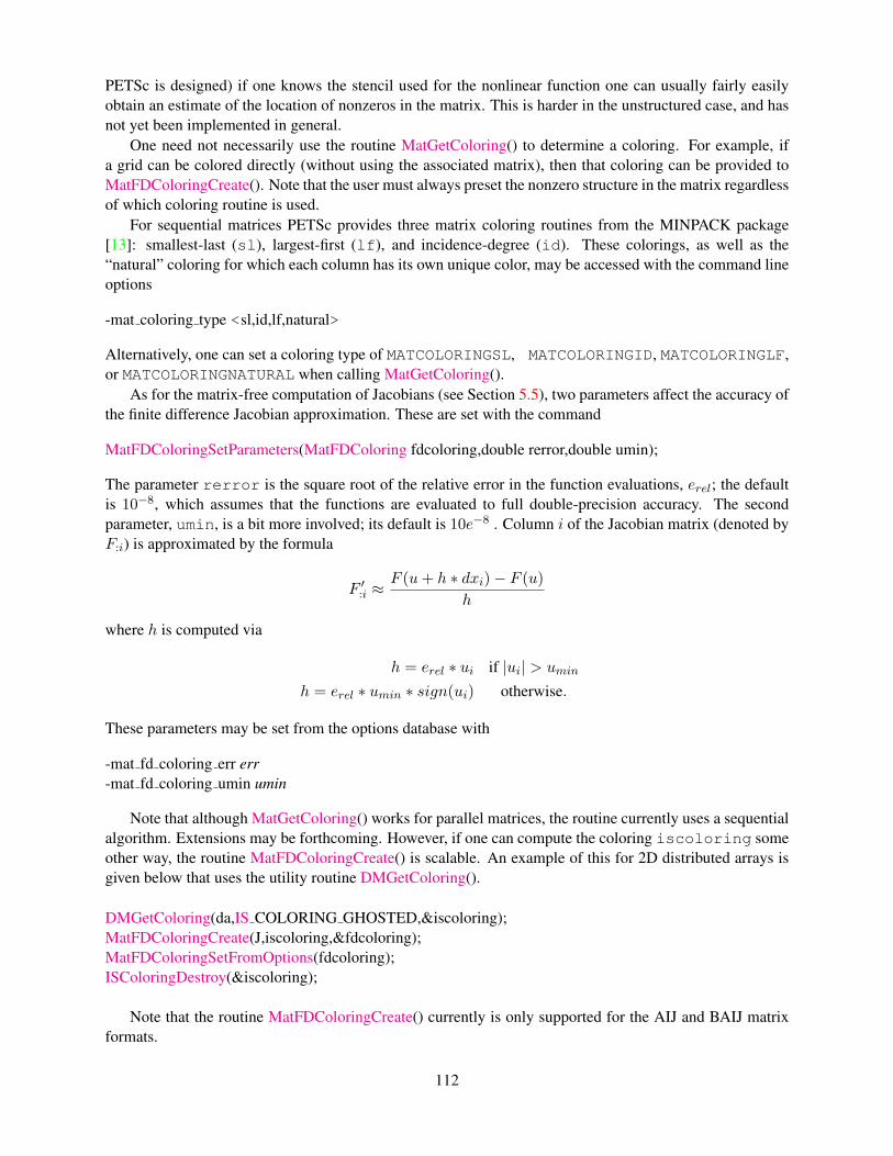
PETSc is designed) if one knows the stencil used for the nonlinear function one can usually fairly easilyobtain an estimate of the location of nonzeros in the matrix. This is harder in the unstructured case, and hasnot yet been implemented in general.
One need not necessarily use the routine MatGetColoring() to determine a coloring. For example, ifa grid can be colored directly (without using the associated matrix), then that coloring can be provided toMatFDColoringCreate(). Note that the user must always preset the nonzero structure in the matrix regardlessof which coloring routine is used.
For sequential matrices PETSc provides three matrix coloring routines from the MINPACK package[13]: smallest-last (sl), largest-first (lf), and incidence-degree (id). These colorings, as well as the“natural” coloring for which each column has its own unique color, may be accessed with the command lineoptions
-mat coloring type <sl,id,lf,natural>
Alternatively, one can set a coloring type of MATCOLORINGSL, MATCOLORINGID, MATCOLORINGLF,or MATCOLORINGNATURAL when calling MatGetColoring().
As for the matrix-free computation of Jacobians (see Section 5.5), two parameters affect the accuracy ofthe finite difference Jacobian approximation. These are set with the command
MatFDColoringSetParameters(MatFDColoring fdcoloring,double rerror,double umin);
The parameter rerror is the square root of the relative error in the function evaluations, erel; the defaultis 10−8, which assumes that the functions are evaluated to full double-precision accuracy. The secondparameter, umin, is a bit more involved; its default is 10e−8 . Column i of the Jacobian matrix (denoted byF:i) is approximated by the formula
F ′:i ≈F (u+ h ∗ dxi)− F (u)
h
where h is computed via
h = erel ∗ ui if |ui| > umin
h = erel ∗ umin ∗ sign(ui) otherwise.
These parameters may be set from the options database with
-mat fd coloring err err-mat fd coloring umin umin
Note that although MatGetColoring() works for parallel matrices, the routine currently uses a sequentialalgorithm. Extensions may be forthcoming. However, if one can compute the coloring iscoloring someother way, the routine MatFDColoringCreate() is scalable. An example of this for 2D distributed arrays isgiven below that uses the utility routine DMGetColoring().
DMGetColoring(da,IS COLORING GHOSTED,&iscoloring);MatFDColoringCreate(J,iscoloring,&fdcoloring);MatFDColoringSetFromOptions(fdcoloring);ISColoringDestroy(&iscoloring);
Note that the routine MatFDColoringCreate() currently is only supported for the AIJ and BAIJ matrixformats.
112
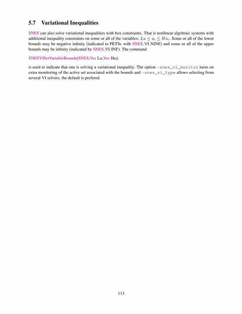
5.7 Variational Inequalities
SNES can also solve variational inequalities with box constraints. That is nonlinear algebraic systems withadditional inequality constraints on some or all of the variables: Lu ≤ ui ≤ Hui. Some or all of the lowerbounds may be negative infinity (indicated to PETSc with SNES VI NINF) and some or all of the upperbounds may be infinity (indicated by SNES VI INF). The command
SNESVISetVariableBounds(SNES,Vec Lu,Vec Hu);
is used to indicate that one is solving a variational inequality. The option -snes_vi_monitor turns onextra monitoring of the active set associated with the bounds and -snes_vi_type allows selecting fromseveral VI solvers, the default is prefered.
113

114
Chapter 6
TS: Scalable ODE and DAE Solvers
The TS library provides a framework for the scalable solution of ODEs and DAEs arising from the dis-cretization of time-dependent PDEs, and of steady-state problems using pseudo-timestepping.
Time-Dependent Problems: Consider the ODE
ut = F (u, t),
where u is a finite-dimensional vector, usually obtained from discretizing a PDE with finite differences,finite elements, etc. For example, in the backward Euler method, discretizing the heat equation
ut = uxx
with centered finite differences results in
(ui)t =ui+1 − 2ui + ui−1
h2;
or with piecewise linear finite elements approximation u(x, t) .=∑
i ξi(t)φi(x) yields semi-discrete equa-tion
Bξ′(t) = Aξ(t)
and discrete equation(B − dtnA)un+1 = Aun,
in whichun
i = ξi(tn) .= u(xi, tn),
ξ′(tn+1) .=un+1
i − uni
dtn,
A is the stiffness matrix and B is the mass matrix.The TS library provides code to solve these equations (currently using the forward or backward Euler
method) as well as an interface to other sophisticated ODE solvers, in a clean and easy manner, where theuser need only provide code for the evaluation of F (u, t) and (optionally) its associated Jacobian matrix.
Steady-State Problems: In addition, TS provides a general code for performing pseudo timestepping witha variable timestep at each physical node point. For example, instead of directly attacking the steady-stateproblem
F (u) = 0,
we can use pseudo-transient continuation by solving
ut = F (u).
115
Using time differencing
ut.=un+1 − un
dtn
with the backward Euler method, we obtain nonlinear equations at a series of pseudo-timesteps
1dtn
B(un+1 − un) = F (un+1).
For this problem the user must provide F (u), the time steps dtn and the left-hand-side matrix B (or op-tionally, if the timestep is position independent and B is the identity matrix, a scalar timestep), as well asoptionally the Jacobian of F (u).
More generally, this can be applied to implicit ODE and DAE for which the transient form is
F (u, u) = 0.
See Section 6.1.2 for details on this formulation.
6.1 Basic TS Usage
The user first creates a TS object with the command
int TSCreate(MPI Comm comm,TSProblemType problemtype,TS *ts);
The TSProblemType is one of TS_LINEAR or TS_NONLINEAR, to indicate whether F (u, t) is given by amatrix A, or A(t), or a function F (u, t).
One can set the solution method with the routine
TSSetType(TS ts,TSType type);
Currently supported types are TSEULER, TSRK (Runge-Kutta), TSBEULER, TSCN (Crank-Nicolson),TSTHETA, TSGL (generalized linear), TSPSEUDO, and TSSUNDIALS (only if the Sundials package isinstalled), or the command line option-ts_type euler,rk,beuler,cn,theta,gl,pseudo,sundials.
Set the initial time and timestep with the command
TSSetInitialTimeStep(TS ts,double time,double dt);
One can change the timestep with the command
TSSetTimeStep(TS ts,double dt);
can determine the current timestep with the routine
TSGetTimeStep(TS ts,double* dt);
Here, “current” refers to the timestep being used to attempt to promote the solution form un to un+1.One sets the total number of timesteps to run or the total time to run (whatever is first) with the command
TSSetDuration(TS ts,int maxsteps,double maxtime);
One performs the request number of time steps with
TSSolve(TS ts,Vec X,PetscReal *ftime);
The solve call implicitly sets up the timestep context; this can be done explicitly with
116
TSSetUp(TS ts);
One destroys the context with
TSDestroy(TS *ts);
and views it with
TSView(TS ts,PetscViewer viewer);
In place of TSSolve(), a single step can be taken using
TSStep(TS ts);
6.1.1 Solving Time-dependent Problems
To set up TS for solving an ODE, one must set the following:
• Solution:
TSSetSolution(TS ts, Vec initialsolution);
The vector initialsolution should contain the “initial conditions” for the ODE.
• Function:
• For linear functions (solved with implicit timestepping), the user must call
TSSetMatrices(TS ts,Mat A,PetscErrorCode (*frhs)(TS,PetscReal,Mat*,Mat*,MatStructure*,void*),Mat B,PetscErrorCode (*flhs)(TS,PetscReal,Mat*,Mat*,MatStructure*,void*),MatStructure flag,void *ctx)
The matrices A and B are right and left hand-side matrix respectively. The functions frhs and flhsare used to form the matrices A and B at each timestep if the matrices are time dependent. If thematrices do not depend on time, the user should pass in PETSC NULL. The variable ctx allowsusers to pass in an application context that is passed to the frhs() or flhs() function wheneverthey are called, as the final argument. The user must provide the matrices A. If B is an identitymatrix, the user should pass in PETSC NULL. If the right-hand side is provided only as a linearfunction, the user must construct a MATSHELL matrix. Note that this is the same interface as that forSNESSetJacobian().
• For nonlinear problems (or linear problems solved using explicit timestepping methods) theuser passes the function with the routine
TSSetRHSFunction(TS ts,Vec R,PetscErrorCode (*f)(TS,double,Vec,Vec,void*),void *fP);
The vector R is an optional location to store the result. The arguments to the function f() are thetimestep context, the current time, the input for the function, the output for the function, and the(optional) user-provided context variable fP.
• Jacobian: For nonlinear problems the user must also provide the (approximate) Jacobian matrix ofF(u,t) and a function to compute it at each Newton iteration. This is done with the command
117
TSSetRHSJacobian(TS ts,Mat A, Mat P,PetscErrorCode (*fjac)(TS,double,Vec,Mat*,Mat*,MatStructure*,void*),void *fP);
The arguments for the function fjac() are the timestep context, the current time, the location wherethe Jacobian is to be computed, the Jacobian matrix, an alternative approximate Jacobian matrix usedas a preconditioner, and the optional user-provided context, passed in as fP. The user must provide theJacobian as a matrix; thus, if using a matrix-free approach is used, the user must create a MATSHELLmatrix. Again, note the similarity to SNESSetJacobian().
Similar to SNESDefaultComputeJacobianColor() is the routine TSDefaultComputeJacobianColor() andTSDefaultComputeJacobian() that corresponds to SNESDefaultComputeJacobian().
6.1.2 Solving Differential Algebraic Equations
The interface for solving time dependent problems given in the implicit form
F (t, u, u) = 0, u(t0) = u0
is slightly different. In general, this is a differential algebraic equation (DAE), but if the matrix Fu(t) =∂F/∂u is nonsingular then it is an ODE and can be transformed to the standard explicit form, although thistransformation may not lead to efficient algorithms. For ODE with nontrivial mass matrices such as arise inFEM, the implicit/DAE interface significantly reduces overhead to prepare the system for algebraic solvers(SNES/KSP) by having the user assemble the correctly shifted matrix. Therefore this interface is also usefulfor ODE systems.
To solve a DAE, instead of TSSetRHSFunction() and TSSetRHSJacobian(), one uses:
• Function F (t, u, u)
TSSetIFunction(TS ts,Vec R,PetscErrorCode (*f)(TS,PetscReal,Vec,Vec,Vec,void*),void *funP);
The vector R is an optional location to store the residual. The arguments to the function f() are thetimestep contex, current time, input state u, input time derivative u, and the (optional) user-providedcontext funP.
• Jacobian Fu + aFu
Unless one is using matrix-free methods without preconditioning, the user must also provide an (ap-proximate) Jacobian matrix of G(u) = F (t, u, w + au). This form for G arises because the timeintegrator internally approximates u by w + au where the positive “shift” a and vector w depend onthe integration method, step size, and past states. The function that evaluates G′(u) = Fu + aFu isset with
TSSetIJacobian(TS ts,Mat A,Mat B,PetscErrorCode (*fjac)(TS,PetscReal,Vec,Vec,PetscReal,Mat*,Mat*,MatStructure*,void*),void *jacP);
The arguments for the function fjac() are the timestep contex, current time, input state u, inputderivative u, shift a, matrix A, preconditioning matrix B, flag describing structure of preconditioningmatrix (see the discussion of KSPSetOperators() in Section 4.1 for details), and the (optional) user-provided context jacP.
118
6.1.3 Using Implicit-Explicit (IMEX) methods for multi-rate problems
The methods of the last section can be generalized for problems with multiple time scales using the form
G(t, u, u) = F (t, u), u(t0) = u0 (6.1)
where G will be treated implicitly using a method suitable for stiff problems and F will be treated explic-itly when using an IMEX method like TSARKIMEX. G is typically linear or weakly nonlinear while Fmay have very strong nonlinearities such as arise in non-oscillatory methods for hyperbolic PDE. The userprovides three pieces of information, the APIs for which have been described above.
• “Slow” part F (t, u) using TSSetRHSFunction().
• “Stiff” part G(t, u, u) using TSSetIFunction().
• Jacobian J(t, u, u) = Gu + aGu using TSSetIJacobian(). An assembled Jacobian is optional and canbe approximated using finite differencing.
To solve Equation 6.1 using fully implicit methods, the user may also provide the Jacobian Fu.
6.1.4 Using Sundials from PETSc
Sundials is a parallel ODE solver developed by Hindmarsh et al. at LLNL. The TS library provides aninterface to use the CVODE component of Sundials directly from PETSc. (To install PETSc to use Sundials,see the installation guide, docs/installation/index.htm.)
To use the Sundials integrators, call
TSSetType(TS ts,TSType TSSUNDIALS);
or use the command line option -ts_type sundials.Sundials’ CVODE solver comes with two main integrator families, Adams and BDF (backward differ-
entiation formula). One can select these with
TSSundialsSetType(TS ts,TSSundialsLmmType [SUNDIALS ADAMS,SUNDIALS BDF]);
or the command line option -ts_sundials_type <adams,bdf>. BDF is the default.Sundials does not use the SNES library within PETSc for its nonlinear solvers, so one cannot change
the nonlinear solver options via SNES. Rather, Sundials uses the preconditioners within the PC package ofPETSc, which can be accessed via
TSSundialsGetPC(TS ts,PC *pc);
The user can then directly set preconditioner options; alternatively, the usual runtime options can be em-ployed via -pc_xxx.
Finally, one can set the Sundials tolerances via
TSSundialsSetTolerance(TS ts,double abs,double rel);
where abs denotes the absolute tolerance and rel the relative tolerance.Other PETSc-Sundials options include
TSSundialsSetGramSchmidtType(TS ts,TSSundialsGramSchmidtType type);
where type is either SUNDIALS_MODIFIED_GS or SUNDIALS_UNMODIFIED_GS. This may be setvia the options data base with -ts_sundials_gramschmidt_type <modifed,unmodified>.
The routine
TSSundialsSetGMRESRestart(TS ts,int restart);
sets the number of vectors in the Krylov subpspace used by GMRES. This may be set in the options databasewith -ts_sundials_gmres_restart restart.
119
6.1.5 Solving Steady-State Problems with Pseudo-Timestepping
For solving steady-state problems with pseudo-timestepping one proceeds as follows.
• Provide the function F(u) with the routine
TSSetRHSFunction(TS ts,PetscErrorCode (*f)(TS,double,Vec,Vec,void*),void *fP);
The arguments to the function f() are the timestep context, the current time, the input for the func-tion, the output for the function and the (optional) user-provided context variable fP.
• Provide the (approximate) Jacobian matrix of F(u,t) and a function to compute it at each Newtoniteration. This is done with the command
TSSetRHSJacobian(TS ts,Mat A, Mat B,PetscErrorCode (*f)(TS,double,Vec,Mat*,Mat*,MatStructure*,void*),void *fP);
The arguments for the function f() are the timestep context, the current time, the location where theJacobian is to be computed, the Jacobian matrix, an alternative approximate Jacobian matrix used asa preconditioner, and the optional user-provided context, passed in as fP. The user must provide theJacobian as a matrix; thus, if using a matrix-free approach, one must create a MATSHELL matrix.
In addition, the user must provide a routine that computes the pseudo-timestep. This is slightly differentdepending on if one is using a constant timestep over the entire grid, or it varies with location.
• For location-independent pseudo-timestepping, one uses the routine
TSPseudoSetTimeStep(TS ts,int(*dt)(TS,double*,void*),void* dtctx);
The function dt is a user-provided function that computes the next pseudo-timestep. As a defaultone can use TSPseudoDefaultTimeStep(TS,double*,void*) for dt. This routine updates the pseudo-timestep with one of two strategies: the default
dtn = dtincrement ∗ dtn−1 ∗ ||F (un−1)||||F (un)||
or, the alternative,
dtn = dtincrement ∗ dt0 ∗||F (u0)||||F (un)||
which can be set with the call
TSPseudoIncrementDtFromInitialDt(TS ts);
or the option -ts_pseudo_increment_dt_from_initial_dt. The value dtincrement is bydefault 1.1, but can be reset with the call
TSPseudoSetTimeStepIncrement(TS ts,double inc);
or the option -ts_pseudo_increment <inc>.
• For location-dependent pseudo-timestepping, the interface function has not yet been created.
120
6.1.6 Using the Explicit Runge-Kutta timestepper with variable timesteps
The Explicit Runge-Kutta timestepper with variable timesteps is an implementation of standard Runge-Kuttausing Dormand-Prince 5(4). It is easy to change this table if needed. Since the time-stepper is using variabletimesteps, the “TSSetInitialTimeStep()” function is not used.
Setting the tolerance with
TSRKSetTolerance(TS ts,double tolerance)
or -ts_rk_tol defines the global tolerance, for the whole time period. The tolerance for each timestep iscalculated relatively to the size of the timestep.
The error in each timestep is calculated using the two solutions given from Dormand-Prince 5(4). Thelocal error is calculated from the 2-norm from the difference of the two solutions.
Other timestep features:
• The next timestep can be maximum 5 times the present timestep
• The smallest timestep can be 1e-14 (to avoid machine precision errors)
More details about the solver and code examples can be found at http://www.parallab.uib.no/projects/molecul/matrix/.
121

122
Chapter 7
High Level Support for Multigrid withDMMG
This infrastructure will be replaced in the next PETSc release. DO NOT USE IT.PETSc provides an easy to use high-level interface for multigrid on a single structured grid using the
PETSc DMDA object (or the DMComposite object) to decompose the grid across the processes. ThisDMMG code is built on top of the lower level PETSc multigrid interface provided in the PCType of MG,see Section 4.4.7. Currently we only provide piecewise linear and piecewise constant interpolation, but canadd more if needed. The DMMG routines only provide linear multigrid but they can be used easily witheither KSP (for linear problems) or SNES (for nonlinear problems).
For linear problems the examples src/ksp/ksp/examples/tutorials/ex22.c and ex25.ccan be used to guide your development. We give a short summary here.
DMMG *dmmg;DM da;Vec soln;/* Create the DMDA that stores information about the coarsest grid you wish to use */ierr = DMDACreate3d(PETSC COMM WORLD,DMDA NONPERIODIC,DMDA STENCIL STAR,3,3,3,PETSC DECIDE,PETSC DECIDE,PETSC DECIDE,1,1,0,0,0,&da);CHKERRQ(ierr);/* Create the DMMG data structure */- the second argument indicates the number of levels you wish to use andcan be changed with the option -dmmg nlevelsierr = DMMGCreate(PETSC COMM WORLD,3,PETSC NULL,&dmmg);CHKERRQ(ierr);/* Tell the DMMG object to use the da to define the coarsest grid */ierr = DMMGSetDM(dmmg,(DM)da);/* Tell the DMMG we are solving a linear problem (hence KSP) and provide thecallback function to compute the right hand side and matrices for each level */ierr = DMMGSetKSP(dmmg,ComputeRHS,ComputeMatrix);CHKERRQ(ierr);/* Solve the problem */ierr = DMMGSolve(dmmg);CHKERRQ(ierr);/* One can access the solution with */soln = DMMGGetx(dmmg);ierr = DMMGDestroy(dmmg);CHKERRQ(ierr);ierr = DMDestroy(&da);CHKERRQ(ierr);
The option -ksp_monitor and -mg_levels_ksp_monitor and optionally -mg_coarse_ksp_monitor causes the DMMG code to print the residual norms for each level of the solver to the screen so
123
that the coarser the grid the more indented the print out. The option -dmmg_grid_sequence causesthe DMMG solve to use grid sequencing to generate the initial guess by solving the same problem on theprevious coarser grid; this often results in a much faster time to solution.
The solver (smoother) used on each level but the coarsest can be controled via the options database withany PC or KSP option prefixed as -mg_levels_[pc/ksp]_. The solver options on the finest grid canbe set with -mg_coarse_[pc/ksp]_. The DMMG has many other options that can view by running theDMMG program with the option -help. You should generally run your code with the option -ksp_viewto see exactly what solvers are being used.
For nonlinear problems one replaces the DMMGSetKSP() with
DMMGSetSNES(DMMG *dmmg,PetscErrorCode (*function)(SNES,Vec,Vec,void*),PetscErrorCode (*jacobian)(SNES,Vec,Mat*,Mat*,MatStructure*,void*))
or the prefered approach
DMMGSetSNESLocal(DMMG *dmmg,PetscErrorCode (*localfunction)(DMDALocalInfo *info,void *x,void *f,void* appctx),PetscErrorCode (*localjacobian)(DMDALocalInfo *,void *x,Mat J,void *appctx),ad function,ad mf function);
The ad_function and ad_mf_function are described in the next chapter. See examples src/snes/examples/tutorials/ex18.c and ex19.c for complete details.
For scalar problems (problems with one degree of freedom per node), the localfunction x andf arguments are simply multi-dimensional arrays of double precision (or complex) numbers (according tothe dimension of the grid) that should be indexed using global i, j, k indices on the entire grid. For multi-component problems you must create a C struct with an entry for each component and the x and f argumentsare appropriately dimensioned arrays of that struct. For example, for a 3d scalar problem the function wouldbe
int localfunction(DMDALocalInfo *info,double ***x, double ***f,void *ctx)
For a 2d multi-component problem with u, v, and p components one would write
typedef struct {PetscScalar u,v,p;} Field;...int localfunction(DMDALocalInfo *info,Field **x,Field **f,void *ctx)
For many nonlinear problems it is too difficult to compute the Jacobian analytically, thus if jacobianor localjacobian is not provided, (indicated by passing in a PETSC NULL) the DMMG will computethe sparse Jacobian reasonably efficiently automatically using finite differencing. See the next chapter oncomputing the Jacobian via automatic differentiation. The option -dmmg_jacobian_mf_fd causes thecode to not compute the Jacobian explicitly but rather to use differences to apply the matrix vector productof the Jacobian.
The usual option -snes_monitor can be used to monitor the progress of the nonlinear solver. Theusual -snes_ options may be used to control the nonlinearr solves. Again we recommend using the option-dmmg_grid_sequence and -snes_view for most runs.
124
Chapter 8
Using ADIC and ADIFOR with PETSc
Automatic differentiation is an incredible technique to generate code that computes Jacobians and otherdifferentives directly from code that only evaluates the function. For structured grid problems, via theDMMG interface (see Chapter 7) PETSc provides a way to use ADIFOR and ADIC to compute the sparseJacobians or perform matrix free vector products with them. See src/snes/examples/tutorials/ex18.c and ex5f.F for example usage.
First one indicates the functions for which one needs Jacobians by adding in the comments in the code
/* Process adiC(maximum number colors): FormFunctionLocal FormFunctionLocali */
where one lists the functions. In Fortran use
! Process adifor: FormFunctionLocal
Next one uses the call
DMMGSetSNESLocal(DMMG *dmmg,PetscErrorCode (*localfunction)(DMDALocalInfo *info,void *x,void *f,void* appctx),PETSC NULL,ad localfunction,ad mf localfunction);
where the names of the last two functions are obtained by prepending an ad_ and ad_mf_ in front of thefunction name. In Fortran, this is done by prepending a g_ and m_.
Two useful options are -dmmg_jacobian_mf_ad and -dmmg_jacobian_mf_ad_operator,with the former is uses the matrix-free automatic differentiation to apply the operator and to define thepreconditioner operator. The latter form uses the matrix-free for the matrix-vector product but still computesthe Jacobian (by default with finite differences) used to construct the preconditioner.
8.1 Work arrays inside the local functions
In C you can call DMDAGetArray() to get work arrays (this is low overhead). In Fortran you can pro-vide a FormFunctionLocal() that had local arrays that have hardwired sizes that are large enough orsomehow allocate space and pass it into an inner FormFunctionLocal() that is the one you differentiate; thissecond approach will require some hand massaging. For example,
subroutine TrueFormFunctionLocal(info,x,f,ctx,ierr)double precision x(gxs:gxe,gys:gye),f(xs:xe,ys:ye)DMDA info(DMDA LOCAL INFO SIZE)integer ctxPetscErrorCode ierr
125

double precision work(gxs:gxe,gys:gye).... do the work ....returnsubroutine FormFunctionLocal(info,x,f,ctx,ierr)double precision x(*),f(*)DMDA info(DMDA LOCAL INFO SIZE)PetscErrorCode ierrinteger ctxdouble precision work(10000)call TrueFormFunctionLocal(info,x,f,work,ctx,ierr)return
126
Chapter 9
Using MATLAB with PETSc
There are four basic ways to use MATLAB with PETSc: (1) dumping files to be read into MATLAB, (2)automatically sending data from a running PETSc program to a MATLAB process where you may inter-actively type MATLAB commands (or run scripts), (3) automatically sending data back and forth betweenPETSc and MATLAB where MATLAB commands are issued not interactively but from a script or thePETSc program and (4) directly in MATLAB using PETSc objects.
9.1 Dumping Data for MATLAB
One can dump PETSc matrices and vectors to the screen (and thus save in a file via > filename.m) ina format that MATLAB can read in directly. This is done with the command line options -vec_view_matlab or -mat_view_matlab. This causes the PETSc program to print the vectors and matrices everytime a VecAssemblyXXX() and MatAssemblyXXX() is called. To provide finer control over when and whatvectors and matrices are dumped one can use the VecView() and MatView() functions with a viewer typeof ASCII (see PetscViewerASCIIOpen(), PETSC_VIEWER_STDOUT_WORLD, PETSC_VIEWER_STDOUT_SELF, or PETSC_VIEWER_STDOUT_(MPI_Comm)). Before calling the viewer set the output typewith, for example,
PetscViewerSetFormat(PETSC VIEWER STDOUT WORLD,PETSC VIEWER ASCII MATLAB);VecView(A,PETSC VIEWER STDOUT WORLD);
or
PetscViewerPushFormat(PETSC VIEWER STDOUT WORLD,PETSC VIEWER ASCII MATLAB);MatView(B,PETSC VIEWER STDOUT WORLD);
The name of each PETSc variable printed for MATLAB may be set with
PetscObjectSetName((PetscObject)A,”name”);
If no name is specified, the object is given a default name using PetscObjectName.
9.2 Sending Data to Interactive Running MATLAB Session
One creates a viewer to MATLAB via
PetscViewerSocketOpen(MPI Comm,char *machine,int port,PetscViewer *v);
(port is usally set to PETSC_DEFAULT, use PETSC NULL for the machine if the MATLAB interactivesession is running on the same machine as the PETSc program) and then sends matrices or vectors via
127
VecView(Vec A,v);MatView(Mat B,v);
One can also send arrays or integer arrays via PetscIntView(), PetscRealView() and PetscScalarView(). Onemay start the MATLAB program manually or use the PETSc command PetscStartMATLAB(MPI_Comm,char *machine,char *script,FILE **fp); where machine and script may be PETSC NULL.
To receive the objects in MATLAB you must first make sure that ${PETSC_DIR}/bin/matlab isin your MATLAB path. Use p = sopen; (or p = sopen(portnum) if you provided a port number inyour call to PetscViewerSocketOpen()), then a = PetscBinaryRead(p); returns the object you havepassed from PETSc. PetscBinaryRead() may be called any number of times. Each call should correspond onthe PETSc side with viewing a single vector or matrix. You many call sclose() to close the connectionfrom MATLAB. It is also possible to start your PETSc program from MATLAB via launch().
9.3 Using the MATLAB Compute Engine
One creates access to the MATLAB engine via
PetscMatlabEngineCreate(MPI Comm comm,char *machine,PetscMatlabEngine *e);
where machine is the name of the machine hosting MATLAB (PETSC NULL may be used for localhost).One can send objects to MATLAB via
PetscMatlabEnginePut(PetscMatlabEngine e,PetscObject obj);
One can get objects via
PetscMatlabEngineGet(PetscMatlabEngine e,PetscObject obj);.
Similarly one can send arrays via
PetscMatlabEnginePutArray(PetscMatlabEngine e,int m,int n,PetscScalar *array,char *name);
and get them back via
PetscMatlabEngineGetArray(PetscMatlabEngine e,int m,int n,PetscScalar *array,char *name);
One cannot use MATLAB interactively in this mode but you can send MATLAB commands via
PetscMatlabEngineEvaluate(PetscMatlabEngine,”format”,...);
where format has the usual printf() format. For example,
PetscMatlabEngineEvaluate(PetscMatlabEngine,”x = %g *y + z;”,avalue);
The name of each PETSc variable passed to Matlab may be set with
PetscObjectSetName((PetscObject)A,”name”);
Text responses can be returned from MATLAB via
PetscMatlabEngineGetOutput(PetscMatlabEngine,char **);
or
PetscMatlabEnginedPrintOutput(PetscMatlabEngine,FILE*).
There is a short-cut to starting the MATLAB engine with PETSC_MATLAB_ENGINE_(MPI_Comm).
128

9.4 Using PETSc objects directly in MATLAB
PETSc must be configured with --with-shared-libraries --with-matlab-engine --with-matlab [--download-f2cblaslapack]. The option --download-f2cblaslapack must beused if using 64bit MATLAB on LINUX or 64bit MATLAB and the --download-ml external packageon Apple Mac OS X. You can build with or without MPI, but cannot run on more than one process There iscurrently no MPI in the API, the MPI Comm is not in any of the argument lists but otherwise the argumentlists try to mimic the C binding. Add ${PETSC_DIR}/bin/matlab/classes to your MATLAB path.
In MATLAB use help PETSc to get started using PETSc from MATLAB once you have setup PETSc tosupport MATLAB.
129

130
Chapter 10
PETSc for Fortran Users
Most of the functionality of PETSc can be obtained by people who program purely in Fortran 77 or Fortran90. The PETSc Fortran interface works with both F77 and F90 compilers.
Since Fortran77 does not provide type checking of routine input/output parameters, we find that many er-rors encountered within PETSc Fortran programs result from accidentally using incorrect calling sequences.Such mistakes are immediately detected during compilation when using C/C++. Thus, using a mixture ofC/C++ and Fortran often works well for programmers who wish to employ Fortran for the core numericalroutines within their applications. In particular, one can effectively write PETSc driver routines in C/C++,thereby preserving flexibility within the program, and still use Fortran when desired for underlying numeri-cal computations. With Fortran 90 compilers we now can provide some type checking from Fortran.
10.1 Differences between PETSc Interfaces for C and Fortran
Only a few differences exist between the C and Fortran PETSc interfaces, all of which are due to Fortran77 syntax limitations. Since PETSc is primarily written in C, the FORTRAN 90 dynamic allocation is noteasily accessible. All Fortran routines have the same names as the corresponding C versions, and PETSccommand line options are fully supported. The routine arguments follow the usual Fortran conventions; theuser need not worry about passing pointers or values. The calling sequences for the Fortran version are inmost cases identical to the C version, except for the error checking variable discussed in Section 10.1.2 anda few routines listed in Section 10.1.10.
10.1.1 Include Files
The Fortran include files for PETSc are located in the directory ${PETSC_DIR}/include/fincludeand should be used via statements such as the following:
#include ”finclude/includefile.h”
Since one must be very careful to include each file no more than once in a Fortran routine, applicationprogrammers must manually include each file needed for the various PETSc libraries within their program.This approach differs from the PETSc C/C++ interface, where the user need only include the highest levelfile, for example, petscsnes.h, which then automatically includes all of the required lower level files.As shown in the examples of Section 10.2, in Fortran one must explicitly list each of the include files. Onemust employ the Fortran file suffix .F rather than .f. This convention enables use of the CPP preprocessor,which allows the use of the #include statements that define PETSc objects and variables. (Familarity withthe CPP preprocessor is not needed for writing PETSc Fortran code; one can simply begin by copying aPETSc Fortran example and its corresponding makefile.)
131
For some of the Fortran 90 functionality of PETSc and type checking of PETSc function calls you canuse
#include ”finclude/includefile.h #include ”finclude/includefile.h90”
See the manual page UsingFortran for how you can use PETSc Fortran module files in your code.
10.1.2 Error Checking
In the Fortran version, each PETSc routine has as its final argument an integer error variable, in contrastto the C convention of providing the error variable as the routine’s return value. The error code is set tobe nonzero if an error has been detected; otherwise, it is zero. For example, the Fortran and C variants ofKSPSolve() are given, respectively, below, where ierr denotes the error variable:
call KSPSolve(KSP ksp,Vec b,Vec x,PetscErrorCode ierr)KSPSolve(KSP ksp,Vec b,Vec x);
Fortran programmers can check these error codes with CHKERRQ(ierr), which terminates all pro-cesses when an error is encountered. Likewise, one can set error codes within Fortran programs by usingSETERRQ(comm,ierr,p,’ ’), which again terminates all processes upon detection of an error. Notethat complete error tracebacks with CHKERRQ() and SETERRQ(), as described in Section 1.4 for C rou-tines, are not directly supported for Fortran routines; however, Fortran programmers can easily use the errorcodes in writing their own tracebacks. For example, one could use code such as the following:
call KSPSolve(ksp,b,x,ierr)if ( ierr .ne. 0) thenprint*, ’Error in routine ...’returnendif
The most common reason for crashing PETSc Fortran code is forgetting the final ierr argument.
10.1.3 Array Arguments
Since Fortran 77 does not allow arrays to be returned in routine arguments, all PETSc routines that returnarrays, such as VecGetArray(), MatGetArray(), ISGetIndices(), and DMDAGetGlobalIndices() are definedslightly differently in Fortran than in C. Instead of returning the array itself, these routines accept as inputa user-specified array of dimension one and return an integer index to the actual array used for data storagewithin PETSc. The Fortran interface for several routines is as follows:
double precision xx v(1), aa v(1)PetscErrorCode ierrinteger ss v(1), dd v(1), nlocPetscOffset ss i, xx i, aa i, dd iVec xMat AIS sDM dcall VecGetArray(x,xx v,xx i,ierr)call MatGetArray(A,aa v,aa i,ierr)call ISGetIndices(s,ss v,ss i,ierr)call DMDAGetGlobalIndices(d,nloc,dd v,dd i,ierr)
132
To access array elements directly, both the user-specified array and the integer index must then be usedtogether. For example, the following Fortran program fragment illustrates directly setting the values ofa vector array instead of using VecSetValues(). Note the (optional) use of the preprocessor #definestatement to enable array manipulations in the conventional Fortran manner.
#define xx a(ib) xx v(xx i + (ib))double precision xx v(1)PetscOffset xx iPetscErrorCode ierrinteger i, nVec xcall VecGetArray(x,xx v,xx i,ierr)call VecGetLocalSize(x,n,ierr)do 10, i=1,nxx a(i) = 3*i + 110 continuecall VecRestoreArray(x,xx v,xx i,ierr)
Figure 17 contains an example of using VecGetArray() within a Fortran routine.Since in this case the array is accessed directly from Fortran, indexing begins with 1, not 0 (unless the
array is declared as xx_v(0:1)). This is different from the use of VecSetValues() where, indexing alwaysstarts with 0.
Note: If using VecGetArray(), MatGetArray(), ISGetIndices(), or DMDAGetGlobalIndices() from For-tran, the user must not compile the Fortran code with options to check for “array entries out of bounds” (e.g.,on the IBM RS/6000 this is done with the -C compiler option, so never use the -C option with this).
10.1.4 Calling Fortran Routines from C (and C Routines from Fortran)
Different machines have different methods of naming Fortran routines called from C (or C routines calledfrom Fortran). Most Fortran compilers change all the capital letters in Fortran routines to small. On somemachines, the Fortran compiler appends an underscore to the end of each Fortran routine name; for example,the Fortran routine Dabsc() would be called from C with dabsc_(). Other machines change all theletters in Fortran routine names to capitals.
PETSc provides two macros (defined in C/C++) to help write portable code that mixes C/C++ and For-tran. They are PETSC_HAVE_FORTRAN_UNDERSCORE and PETSC_HAVE_FORTRAN_CAPS , whichare defined in the file ${PETSC_DIR}/${PETSC_ARCH}/include/petscconf.h. The macros areused, for example, as follows:
#if defined(PETSC HAVE FORTRAN CAPS)#define dabsc DMDABSC#elif !defined(PETSC HAVE FORTRAN UNDERSCORE)#define dabsc dabsc#endif.....dabsc (&n,x,y); /* call the Fortran function */
10.1.5 Passing Null Pointers
In several PETSc C functions, one has the option of passing a 0 (null) argument (for example, the fifthargument of MatCreateSeqAIJ()). From Fortran, users must pass PETSC_NULL_XXX to indicate a null ar-gument (where XXX is INTEGER, DOUBLE, CHARACTER, or SCALAR depending on the type of argument
133
required); passing 0 from Fortran will crash the code. Note that the C convention of passing PETSC NULL(or 0) cannot be used. For example, when no options prefix is desired in the routine PetscOptionsGetInt(),one must use the following command in Fortran:
call PetscOptionsGetInt(PETSC NULL CHARACTER,’-name’,N,flg,ierr)
This Fortran requirement is inconsistent with C, where the user can employ PETSC NULL for all nullarguments.
10.1.6 Duplicating Multiple Vectors
The Fortran interface to VecDuplicateVecs() differs slightly from the C/C++ variant because Fortran doesnot allow arrays to be returned in routine arguments. To create n vectors of the same format as an existingvector, the user must declare a vector array, v_new of size n. Then, after VecDuplicateVecs() has beencalled, v_new will contain (pointers to) the new PETSc vector objects. When finished with the vectors, theuser should destroy them by calling VecDestroyVecs(). For example, the following code fragment duplicatesv_old to form two new vectors, v_new(1) and v_new(2).
Vec v old, v new(2)integer ierrPetscScalar alpha....call VecDuplicateVecs(v old,2,v new,ierr)alpha = 4.3call VecSet(v new(1),alpha,ierr)alpha = 6.0call VecSet(v new(2),alpha,ierr)....call VecDestroyVecs(2,&v new,ierr)
10.1.7 Matrix, Vector and IS Indices
All matrices, vectors and IS in PETSc use zero-based indexing, regardless of whether C or Fortran is beingused. The interface routines, such as MatSetValues() and VecSetValues(), always use zero indexing. SeeSection 3.2 for further details.
10.1.8 Setting Routines
When a function pointer is passed as an argument to a PETSc function, such as the test in KSPSetConver-genceTest(), it is assumed that this pointer references a routine written in the same language as the PETScinterface function that was called. For instance, if KSPSetConvergenceTest() is called from C, the test argu-ment is assumed to be a C function. Likewise, if it is called from Fortran, the test is assumed to be writtenin Fortran.
10.1.9 Compiling and Linking Fortran Programs
Figure 23 shows a sample makefile that can be used for PETSc programs. In this makefile, one can compileand run a debugging version of the Fortran program ex3.Fwith the actions make ex3 and make runex3,respectively. The compilation command is restated below:
134
ex3: ex3.o-${FLINKER} -o ex3 ex3.o ${PETSC_LIB}${RM} ex3.o
10.1.10 Routines with Different Fortran Interfaces
The following Fortran routines differ slightly from their C counterparts; see the manual pages and previousdiscussion in this chapter for details:
PetscInitialize(char *filename,int ierr)PetscError(MPI COMM,int err,char *message,int ierr)VecGetArray(), MatGetArray()ISGetIndices(), DMDAGetGlobalIndices()VecDuplicateVecs(), VecDestroyVecs()PetscOptionsGetString()
The following functions are not supported in Fortran:
PetscFClose(), PetscFOpen(), PetscFPrintf(), PetscPrintf()PetscPopErrorHandler(), PetscPushErrorHandler()PetscInfo()PetscSetDebugger()VecGetArrays(), VecRestoreArrays()PetscViewerASCIIGetPointer(), PetscViewerBinaryGetDescriptor()PetscViewerStringOpen(), PetscViewerStringSPrintf()PetscOptionsGetStringArray()
10.1.11 Fortran90
PETSc includes limited support for direct use of Fortran90 pointers. Current routines include:
VecGetArrayF90(), VecRestoreArrayF90()VecDuplicateVecsF90(), VecDestroyVecsF90()DMDAGetGlobalIndicesF90()MatGetArrayF90(), MatRestoreArrayF90()ISGetIndicesF90(), ISRestoreIndicesF90()
See the manual pages for details and pointers to example programs. To use the routines VecGetArrayF90(),VecRestoreArrayF90() VecDuplicateVecsF90(), and VecDestroyVecsF90(), one must use the Fortran90 vec-tor include file,
#include ”finclude/petscvec.h90”
Analogous include files for other libraries are petscdm.h90, petscmat.h90, and petscis.h90.Unfortunately, these routines currently work only on certain machines with certain compilers. They
currently work with the SGI, Solaris, the Cray T3E, the IBM and the NAG Fortran 90 compiler.
10.2 Sample Fortran77 Programs
Sample programs that illustrate the PETSc interface for Fortran are given in Figures 16 – 19, correspondingto ${PETSC_DIR}/src/vec/vec/examples/tests/ex19f.F, ${PETSC_DIR}/src/vec/vec/examples/tutorials/ex4f.F,
135
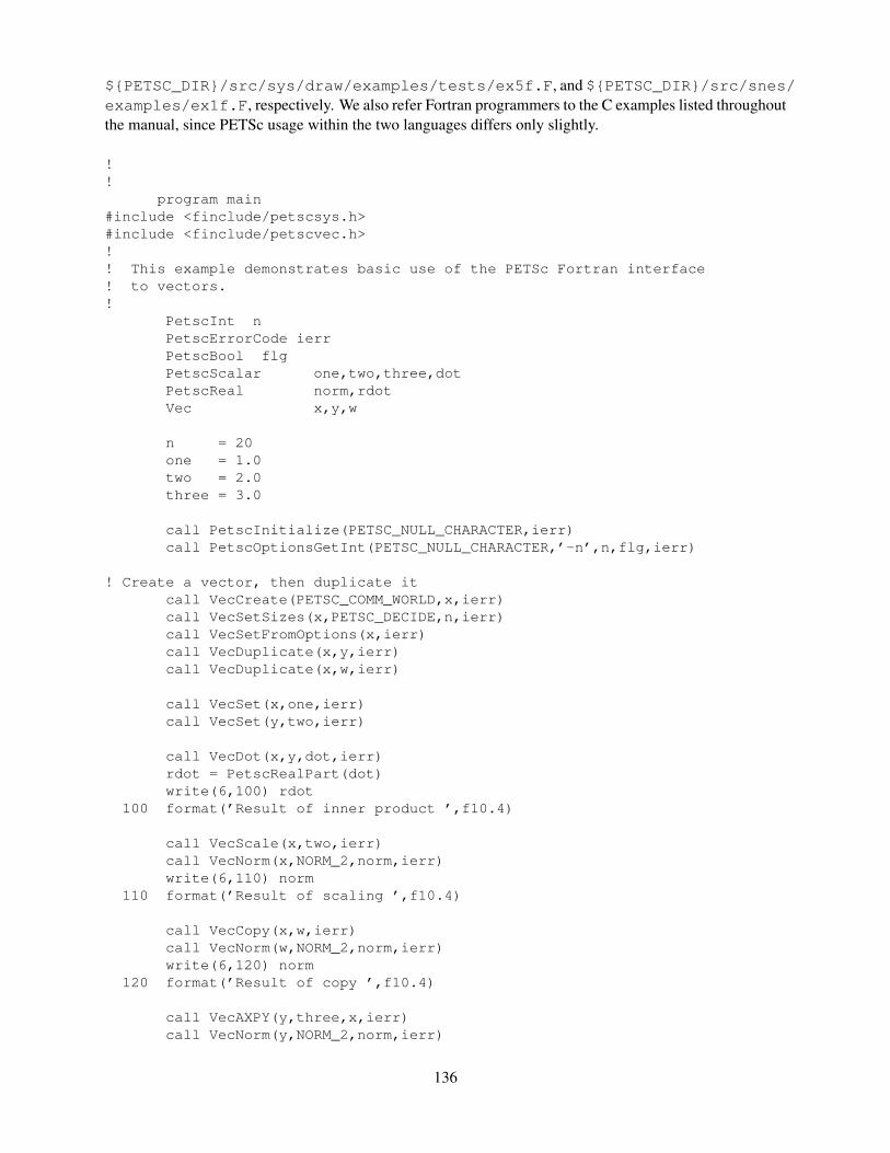
${PETSC_DIR}/src/sys/draw/examples/tests/ex5f.F, and ${PETSC_DIR}/src/snes/examples/ex1f.F, respectively. We also refer Fortran programmers to the C examples listed throughoutthe manual, since PETSc usage within the two languages differs only slightly.
!!
program main#include <finclude/petscsys.h>#include <finclude/petscvec.h>!! This example demonstrates basic use of the PETSc Fortran interface! to vectors.!
PetscInt nPetscErrorCode ierrPetscBool flgPetscScalar one,two,three,dotPetscReal norm,rdotVec x,y,w
n = 20one = 1.0two = 2.0three = 3.0
call PetscInitialize(PETSC_NULL_CHARACTER,ierr)call PetscOptionsGetInt(PETSC_NULL_CHARACTER,’-n’,n,flg,ierr)
! Create a vector, then duplicate itcall VecCreate(PETSC_COMM_WORLD,x,ierr)call VecSetSizes(x,PETSC_DECIDE,n,ierr)call VecSetFromOptions(x,ierr)call VecDuplicate(x,y,ierr)call VecDuplicate(x,w,ierr)
call VecSet(x,one,ierr)call VecSet(y,two,ierr)
call VecDot(x,y,dot,ierr)rdot = PetscRealPart(dot)write(6,100) rdot
100 format(’Result of inner product ’,f10.4)
call VecScale(x,two,ierr)call VecNorm(x,NORM_2,norm,ierr)write(6,110) norm
110 format(’Result of scaling ’,f10.4)
call VecCopy(x,w,ierr)call VecNorm(w,NORM_2,norm,ierr)write(6,120) norm
120 format(’Result of copy ’,f10.4)
call VecAXPY(y,three,x,ierr)call VecNorm(y,NORM_2,norm,ierr)
136
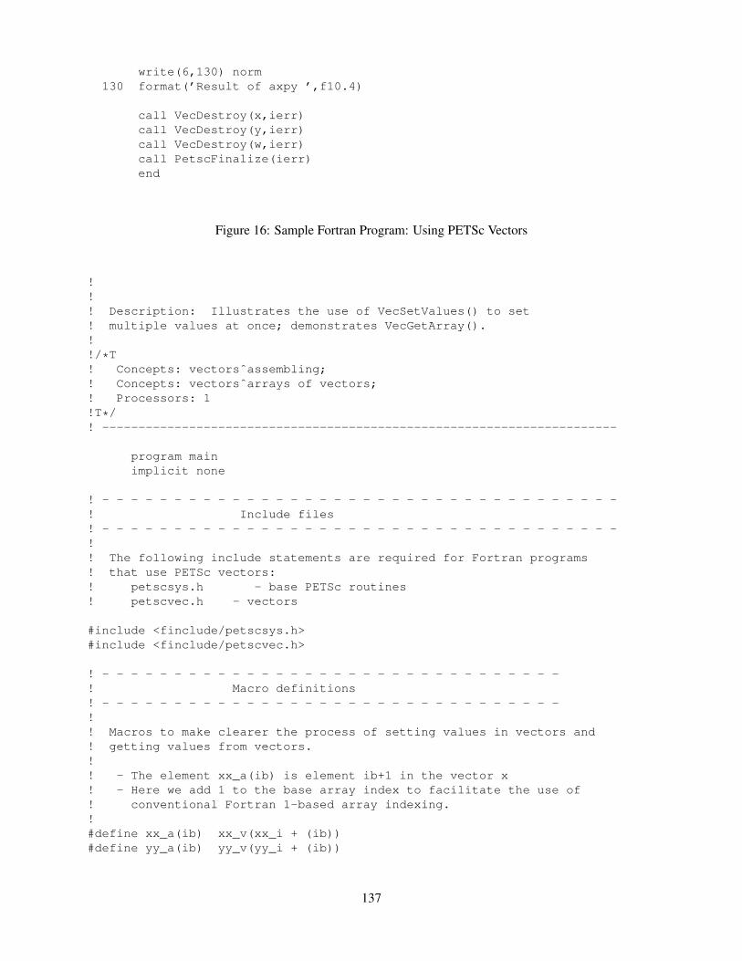
write(6,130) norm130 format(’Result of axpy ’,f10.4)
call VecDestroy(x,ierr)call VecDestroy(y,ierr)call VecDestroy(w,ierr)call PetscFinalize(ierr)end
Figure 16: Sample Fortran Program: Using PETSc Vectors
!!! Description: Illustrates the use of VecSetValues() to set! multiple values at once; demonstrates VecGetArray().!!/*T! Concepts: vectorsˆassembling;! Concepts: vectorsˆarrays of vectors;! Processors: 1!T*/! -----------------------------------------------------------------------
program mainimplicit none
! - - - - - - - - - - - - - - - - - - - - - - - - - - - - - - - - - - - -! Include files! - - - - - - - - - - - - - - - - - - - - - - - - - - - - - - - - - - - -!! The following include statements are required for Fortran programs! that use PETSc vectors:! petscsys.h - base PETSc routines! petscvec.h - vectors
#include <finclude/petscsys.h>#include <finclude/petscvec.h>
! - - - - - - - - - - - - - - - - - - - - - - - - - - - - - - - -! Macro definitions! - - - - - - - - - - - - - - - - - - - - - - - - - - - - - - - -!! Macros to make clearer the process of setting values in vectors and! getting values from vectors.!! - The element xx_a(ib) is element ib+1 in the vector x! - Here we add 1 to the base array index to facilitate the use of! conventional Fortran 1-based array indexing.!#define xx_a(ib) xx_v(xx_i + (ib))#define yy_a(ib) yy_v(yy_i + (ib))
137
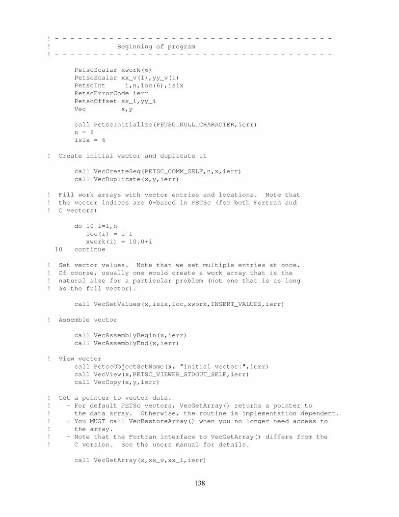
! - - - - - - - - - - - - - - - - - - - - - - - - - - - - - - - - - - - -! Beginning of program! - - - - - - - - - - - - - - - - - - - - - - - - - - - - - - - - - - - -
PetscScalar xwork(6)PetscScalar xx_v(1),yy_v(1)PetscInt i,n,loc(6),isixPetscErrorCode ierrPetscOffset xx_i,yy_iVec x,y
call PetscInitialize(PETSC_NULL_CHARACTER,ierr)n = 6isix = 6
! Create initial vector and duplicate it
call VecCreateSeq(PETSC_COMM_SELF,n,x,ierr)call VecDuplicate(x,y,ierr)
! Fill work arrays with vector entries and locations. Note that! the vector indices are 0-based in PETSc (for both Fortran and! C vectors)
do 10 i=1,nloc(i) = i-1xwork(i) = 10.0*i
10 continue
! Set vector values. Note that we set multiple entries at once.! Of course, usually one would create a work array that is the! natural size for a particular problem (not one that is as long! as the full vector).
call VecSetValues(x,isix,loc,xwork,INSERT_VALUES,ierr)
! Assemble vector
call VecAssemblyBegin(x,ierr)call VecAssemblyEnd(x,ierr)
! View vectorcall PetscObjectSetName(x, "initial vector:",ierr)call VecView(x,PETSC_VIEWER_STDOUT_SELF,ierr)call VecCopy(x,y,ierr)
! Get a pointer to vector data.! - For default PETSc vectors, VecGetArray() returns a pointer to! the data array. Otherwise, the routine is implementation dependent.! - You MUST call VecRestoreArray() when you no longer need access to! the array.! - Note that the Fortran interface to VecGetArray() differs from the! C version. See the users manual for details.
call VecGetArray(x,xx_v,xx_i,ierr)
138
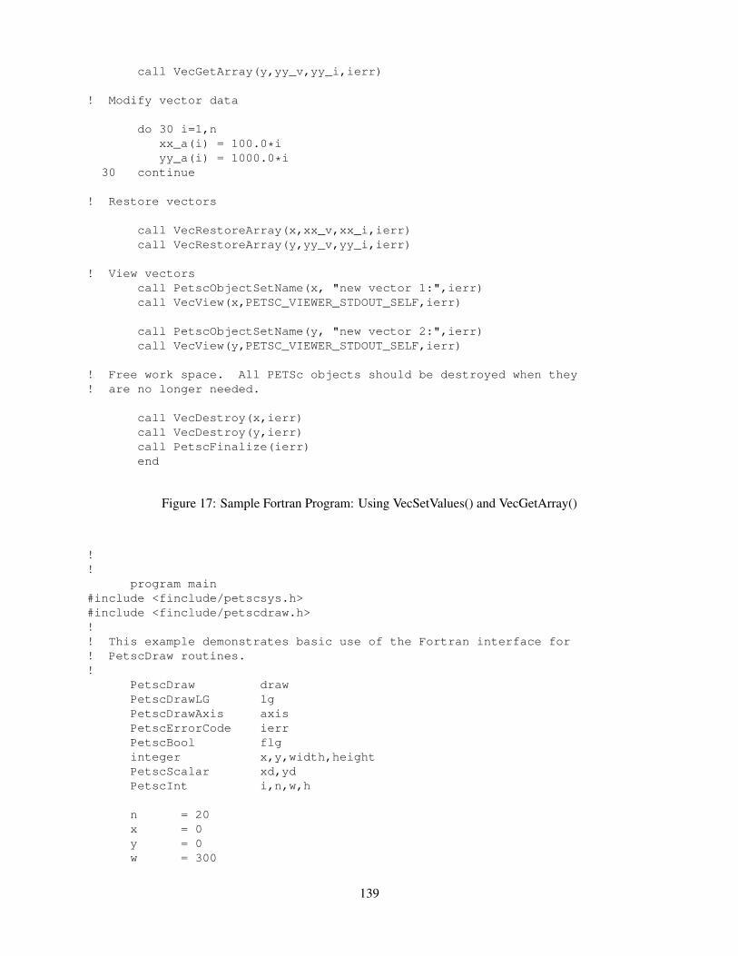
call VecGetArray(y,yy_v,yy_i,ierr)
! Modify vector data
do 30 i=1,nxx_a(i) = 100.0*iyy_a(i) = 1000.0*i
30 continue
! Restore vectors
call VecRestoreArray(x,xx_v,xx_i,ierr)call VecRestoreArray(y,yy_v,yy_i,ierr)
! View vectorscall PetscObjectSetName(x, "new vector 1:",ierr)call VecView(x,PETSC_VIEWER_STDOUT_SELF,ierr)
call PetscObjectSetName(y, "new vector 2:",ierr)call VecView(y,PETSC_VIEWER_STDOUT_SELF,ierr)
! Free work space. All PETSc objects should be destroyed when they! are no longer needed.
call VecDestroy(x,ierr)call VecDestroy(y,ierr)call PetscFinalize(ierr)end
Figure 17: Sample Fortran Program: Using VecSetValues() and VecGetArray()
!!
program main#include <finclude/petscsys.h>#include <finclude/petscdraw.h>!! This example demonstrates basic use of the Fortran interface for! PetscDraw routines.!
PetscDraw drawPetscDrawLG lgPetscDrawAxis axisPetscErrorCode ierrPetscBool flginteger x,y,width,heightPetscScalar xd,ydPetscInt i,n,w,h
n = 20x = 0y = 0w = 300
139
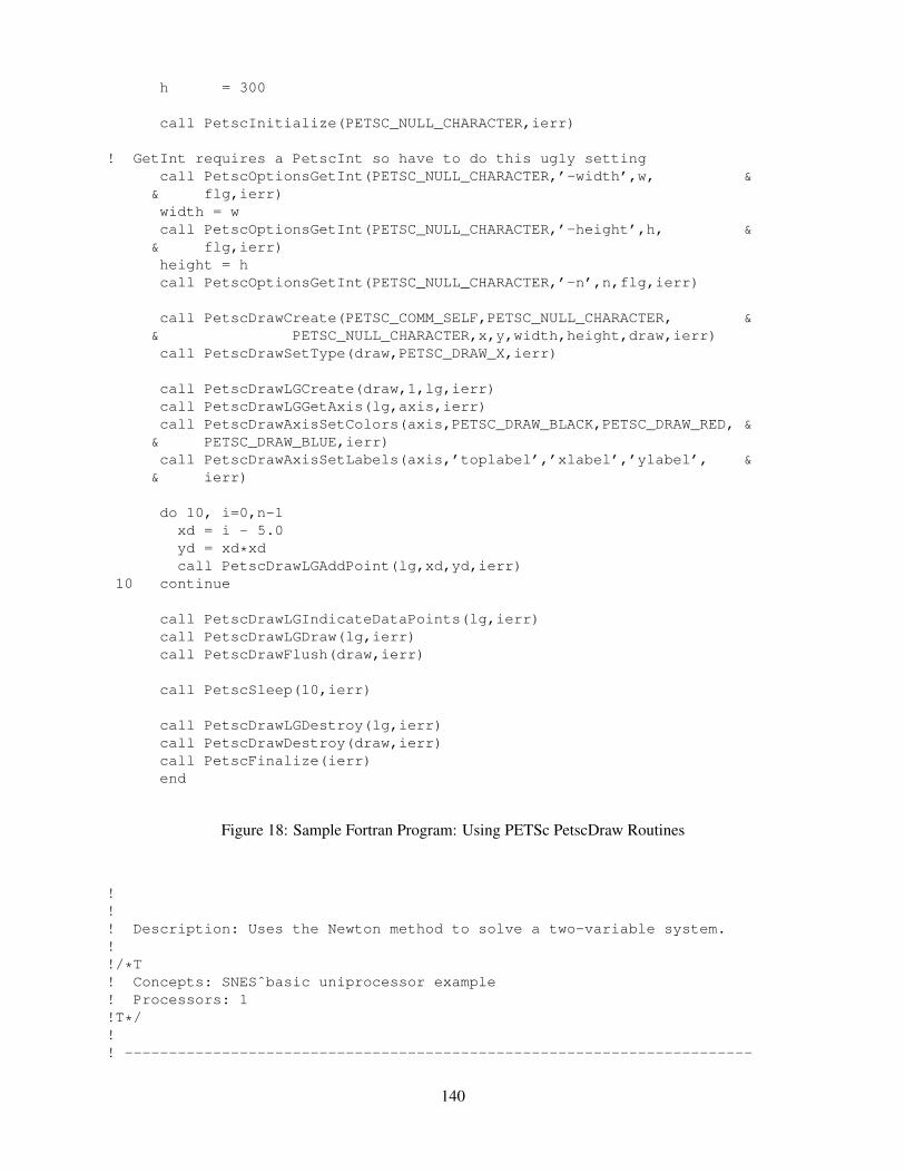
h = 300
call PetscInitialize(PETSC_NULL_CHARACTER,ierr)
! GetInt requires a PetscInt so have to do this ugly settingcall PetscOptionsGetInt(PETSC_NULL_CHARACTER,’-width’,w, && flg,ierr)width = wcall PetscOptionsGetInt(PETSC_NULL_CHARACTER,’-height’,h, && flg,ierr)height = hcall PetscOptionsGetInt(PETSC_NULL_CHARACTER,’-n’,n,flg,ierr)
call PetscDrawCreate(PETSC_COMM_SELF,PETSC_NULL_CHARACTER, && PETSC_NULL_CHARACTER,x,y,width,height,draw,ierr)call PetscDrawSetType(draw,PETSC_DRAW_X,ierr)
call PetscDrawLGCreate(draw,1,lg,ierr)call PetscDrawLGGetAxis(lg,axis,ierr)call PetscDrawAxisSetColors(axis,PETSC_DRAW_BLACK,PETSC_DRAW_RED, && PETSC_DRAW_BLUE,ierr)call PetscDrawAxisSetLabels(axis,’toplabel’,’xlabel’,’ylabel’, && ierr)
do 10, i=0,n-1xd = i - 5.0yd = xd*xdcall PetscDrawLGAddPoint(lg,xd,yd,ierr)
10 continue
call PetscDrawLGIndicateDataPoints(lg,ierr)call PetscDrawLGDraw(lg,ierr)call PetscDrawFlush(draw,ierr)
call PetscSleep(10,ierr)
call PetscDrawLGDestroy(lg,ierr)call PetscDrawDestroy(draw,ierr)call PetscFinalize(ierr)end
Figure 18: Sample Fortran Program: Using PETSc PetscDraw Routines
!!! Description: Uses the Newton method to solve a two-variable system.!!/*T! Concepts: SNESˆbasic uniprocessor example! Processors: 1!T*/!! -----------------------------------------------------------------------
140
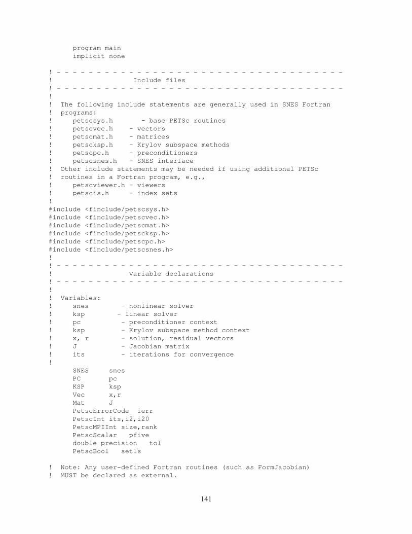
program mainimplicit none
! - - - - - - - - - - - - - - - - - - - - - - - - - - - - - - - - - - - -! Include files! - - - - - - - - - - - - - - - - - - - - - - - - - - - - - - - - - - - -!! The following include statements are generally used in SNES Fortran! programs:! petscsys.h - base PETSc routines! petscvec.h - vectors! petscmat.h - matrices! petscksp.h - Krylov subspace methods! petscpc.h - preconditioners! petscsnes.h - SNES interface! Other include statements may be needed if using additional PETSc! routines in a Fortran program, e.g.,! petscviewer.h - viewers! petscis.h - index sets!#include <finclude/petscsys.h>#include <finclude/petscvec.h>#include <finclude/petscmat.h>#include <finclude/petscksp.h>#include <finclude/petscpc.h>#include <finclude/petscsnes.h>!! - - - - - - - - - - - - - - - - - - - - - - - - - - - - - - - - - - - -! Variable declarations! - - - - - - - - - - - - - - - - - - - - - - - - - - - - - - - - - - - -!! Variables:! snes - nonlinear solver! ksp - linear solver! pc - preconditioner context! ksp - Krylov subspace method context! x, r - solution, residual vectors! J - Jacobian matrix! its - iterations for convergence!
SNES snesPC pcKSP kspVec x,rMat JPetscErrorCode ierrPetscInt its,i2,i20PetscMPIInt size,rankPetscScalar pfivedouble precision tolPetscBool setls
! Note: Any user-defined Fortran routines (such as FormJacobian)! MUST be declared as external.
141
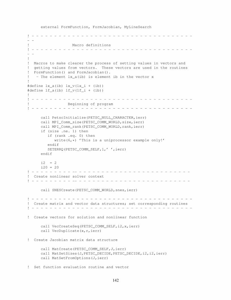
external FormFunction, FormJacobian, MyLineSearch
! - - - - - - - - - - - - - - - - - - - - - - - - - - - - - - - - - - - -- -! Macro definitions! - - - - - - - - - - - - - - - - - - - - - - - - - - - - - - - - - - - -- -!! Macros to make clearer the process of setting values in vectors and! getting values from vectors. These vectors are used in the routines! FormFunction() and FormJacobian().! - The element lx_a(ib) is element ib in the vector x!#define lx_a(ib) lx_v(lx_i + (ib))#define lf_a(ib) lf_v(lf_i + (ib))!! - - - - - - - - - - - - - - - - - - - - - - - - - - - - - - - - - - - -! Beginning of program! - - - - - - - - - - - - - - - - - - - - - - - - - - - - - - - - - - - -
call PetscInitialize(PETSC_NULL_CHARACTER,ierr)call MPI_Comm_size(PETSC_COMM_WORLD,size,ierr)call MPI_Comm_rank(PETSC_COMM_WORLD,rank,ierr)if (size .ne. 1) then
if (rank .eq. 0) thenwrite(6,*) ’This is a uniprocessor example only!’
endifSETERRQ(PETSC_COMM_SELF,1,’ ’,ierr)
endif
i2 = 2i20 = 20
! - - - - - - - - - -- - - - - - - - - - - - - - - - - - - - - - - - - -! Create nonlinear solver context! - - - - - - - - - -- - - - - - - - - - - - - - - - - - - - - - - - - -
call SNESCreate(PETSC_COMM_WORLD,snes,ierr)
! - - - - - - - - - - - - - - - - - - - - - - - - - - - - - - - - - - - -! Create matrix and vector data structures; set corresponding routines! - - - - - - - - - - - - - - - - - - - - - - - - - - - - - - - - - - - -
! Create vectors for solution and nonlinear function
call VecCreateSeq(PETSC_COMM_SELF,i2,x,ierr)call VecDuplicate(x,r,ierr)
! Create Jacobian matrix data structure
call MatCreate(PETSC_COMM_SELF,J,ierr)call MatSetSizes(J,PETSC_DECIDE,PETSC_DECIDE,i2,i2,ierr)call MatSetFromOptions(J,ierr)
! Set function evaluation routine and vector
142
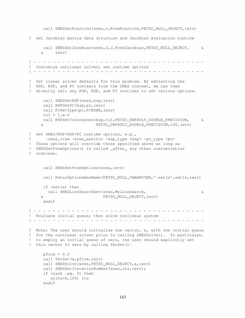
call SNESSetFunction(snes,r,FormFunction,PETSC_NULL_OBJECT,ierr)
! Set Jacobian matrix data structure and Jacobian evaluation routine
call SNESSetJacobian(snes,J,J,FormJacobian,PETSC_NULL_OBJECT, && ierr)
! - - - - - - - - - - - - - - - - - - - - - - - - - - - - - - - - - - - -! Customize nonlinear solver; set runtime options! - - - - - - - - - - - - - - - - - - - - - - - - - - - - - - - - - - - -
! Set linear solver defaults for this problem. By extracting the! KSP, KSP, and PC contexts from the SNES context, we can then! directly call any KSP, KSP, and PC routines to set various options.
call SNESGetKSP(snes,ksp,ierr)call KSPGetPC(ksp,pc,ierr)call PCSetType(pc,PCNONE,ierr)tol = 1.e-4call KSPSetTolerances(ksp,tol,PETSC_DEFAULT_DOUBLE_PRECISION, &
& PETSC_DEFAULT_DOUBLE_PRECISION,i20,ierr)
! Set SNES/KSP/KSP/PC runtime options, e.g.,! -snes_view -snes_monitor -ksp_type <ksp> -pc_type <pc>! These options will override those specified above as long as! SNESSetFromOptions() is called _after_ any other customization! routines.
call SNESSetFromOptions(snes,ierr)
call PetscOptionsHasName(PETSC_NULL_CHARACTER,’-setls’,setls,ierr)
if (setls) thencall SNESLineSearchSet(snes,MyLineSearch, &
& PETSC_NULL_OBJECT,ierr)endif
! - - - - - - - - - - - - - - - - - - - - - - - - - - - - - - - - - - - -! Evaluate initial guess; then solve nonlinear system! - - - - - - - - - - - - - - - - - - - - - - - - - - - - - - - - - - - -
! Note: The user should initialize the vector, x, with the initial guess! for the nonlinear solver prior to calling SNESSolve(). In particular,! to employ an initial guess of zero, the user should explicitly set! this vector to zero by calling VecSet().
pfive = 0.5call VecSet(x,pfive,ierr)call SNESSolve(snes,PETSC_NULL_OBJECT,x,ierr)call SNESGetIterationNumber(snes,its,ierr);if (rank .eq. 0) then
write(6,100) itsendif
143
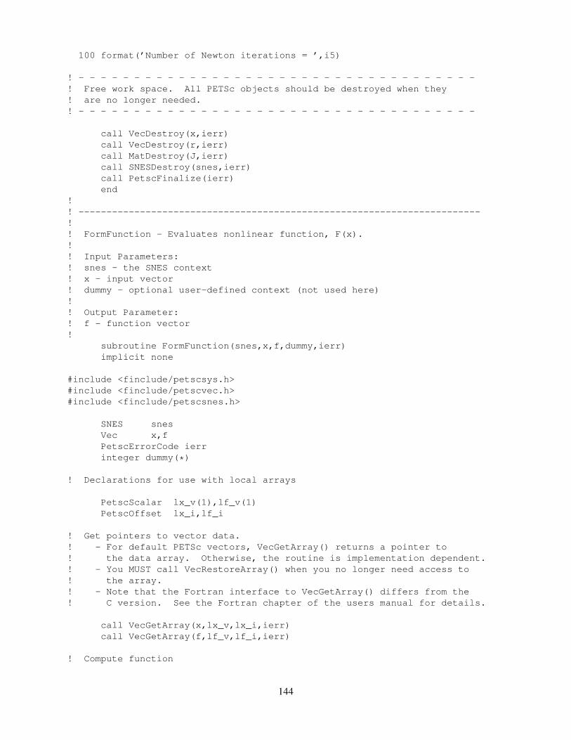
100 format(’Number of Newton iterations = ’,i5)
! - - - - - - - - - - - - - - - - - - - - - - - - - - - - - - - - - - - -! Free work space. All PETSc objects should be destroyed when they! are no longer needed.! - - - - - - - - - - - - - - - - - - - - - - - - - - - - - - - - - - - -
call VecDestroy(x,ierr)call VecDestroy(r,ierr)call MatDestroy(J,ierr)call SNESDestroy(snes,ierr)call PetscFinalize(ierr)end
!! ------------------------------------------------------------------------!! FormFunction - Evaluates nonlinear function, F(x).!! Input Parameters:! snes - the SNES context! x - input vector! dummy - optional user-defined context (not used here)!! Output Parameter:! f - function vector!
subroutine FormFunction(snes,x,f,dummy,ierr)implicit none
#include <finclude/petscsys.h>#include <finclude/petscvec.h>#include <finclude/petscsnes.h>
SNES snesVec x,fPetscErrorCode ierrinteger dummy(*)
! Declarations for use with local arrays
PetscScalar lx_v(1),lf_v(1)PetscOffset lx_i,lf_i
! Get pointers to vector data.! - For default PETSc vectors, VecGetArray() returns a pointer to! the data array. Otherwise, the routine is implementation dependent.! - You MUST call VecRestoreArray() when you no longer need access to! the array.! - Note that the Fortran interface to VecGetArray() differs from the! C version. See the Fortran chapter of the users manual for details.
call VecGetArray(x,lx_v,lx_i,ierr)call VecGetArray(f,lf_v,lf_i,ierr)
! Compute function
144
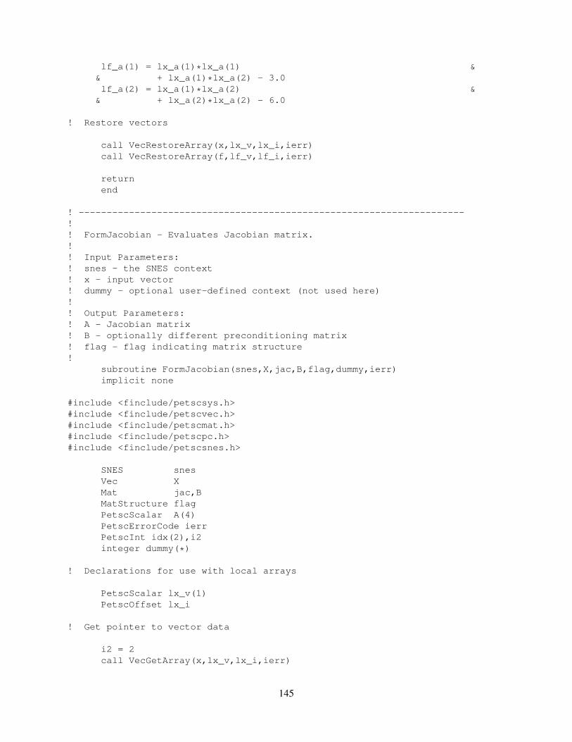
lf_a(1) = lx_a(1)*lx_a(1) && + lx_a(1)*lx_a(2) - 3.0lf_a(2) = lx_a(1)*lx_a(2) &
& + lx_a(2)*lx_a(2) - 6.0
! Restore vectors
call VecRestoreArray(x,lx_v,lx_i,ierr)call VecRestoreArray(f,lf_v,lf_i,ierr)
returnend
! ---------------------------------------------------------------------!! FormJacobian - Evaluates Jacobian matrix.!! Input Parameters:! snes - the SNES context! x - input vector! dummy - optional user-defined context (not used here)!! Output Parameters:! A - Jacobian matrix! B - optionally different preconditioning matrix! flag - flag indicating matrix structure!
subroutine FormJacobian(snes,X,jac,B,flag,dummy,ierr)implicit none
#include <finclude/petscsys.h>#include <finclude/petscvec.h>#include <finclude/petscmat.h>#include <finclude/petscpc.h>#include <finclude/petscsnes.h>
SNES snesVec XMat jac,BMatStructure flagPetscScalar A(4)PetscErrorCode ierrPetscInt idx(2),i2integer dummy(*)
! Declarations for use with local arrays
PetscScalar lx_v(1)PetscOffset lx_i
! Get pointer to vector data
i2 = 2call VecGetArray(x,lx_v,lx_i,ierr)
145
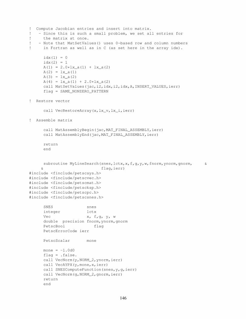
! Compute Jacobian entries and insert into matrix.! - Since this is such a small problem, we set all entries for! the matrix at once.! - Note that MatSetValues() uses 0-based row and column numbers! in Fortran as well as in C (as set here in the array idx).
idx(1) = 0idx(2) = 1A(1) = 2.0*lx_a(1) + lx_a(2)A(2) = lx_a(1)A(3) = lx_a(2)A(4) = lx_a(1) + 2.0*lx_a(2)call MatSetValues(jac,i2,idx,i2,idx,A,INSERT_VALUES,ierr)flag = SAME_NONZERO_PATTERN
! Restore vector
call VecRestoreArray(x,lx_v,lx_i,ierr)
! Assemble matrix
call MatAssemblyBegin(jac,MAT_FINAL_ASSEMBLY,ierr)call MatAssemblyEnd(jac,MAT_FINAL_ASSEMBLY,ierr)
returnend
subroutine MyLineSearch(snes,lctx,x,f,g,y,w,fnorm,ynorm,gnorm, && flag,ierr)
#include <finclude/petscsys.h>#include <finclude/petscvec.h>#include <finclude/petscmat.h>#include <finclude/petscksp.h>#include <finclude/petscpc.h>#include <finclude/petscsnes.h>
SNES snesinteger lctxVec x, f,g, y, wdouble precision fnorm,ynorm,gnormPetscBool flagPetscErrorCode ierr
PetscScalar mone
mone = -1.0d0flag = .false.call VecNorm(y,NORM_2,ynorm,ierr)call VecAYPX(y,mone,x,ierr)call SNESComputeFunction(snes,y,g,ierr)call VecNorm(g,NORM_2,gnorm,ierr)returnend
146

Figure 19: Sample Fortran Program: Using PETSc Nonlinear Solvers
147

148

Part III
Additional Information
149

Chapter 11
Profiling
PETSc includes a consistent, lightweight scheme to allow the profiling of application programs. The PETScroutines automatically log performance data if certain options are specified at runtime. The user can alsolog information about application codes for a complete picture of performance. In addition, as describedin Section 11.1.1, PETSc provides a mechanism for printing informative messages about computations.Section 11.1 introduces the various profiling options in PETSc, while the remainder of the chapter focuseson details such as monitoring application codes and tips for accurate profiling.
11.1 Basic Profiling Information
If an application code and the PETSc libraries have been configured with --with-debugging=1, thedefault, then various kinds of profiling of code between calls to PetscInitialize() and PetscFinalize() can beactivated at runtime. The profiling options include the following:
• -log_summary - Prints an ASCII version of performance data at program’s conclusion. Thesestatistics are comprehensive and concise and require little overhead; thus, -log_summary is in-tended as the primary means of monitoring the performance of PETSc codes.
• -info [infofile] - Prints verbose information about code to stdout or an optional file. Thisoption provides details about algorithms, data structures, etc. Since the overhead of printing suchoutput slows a code, this option should not be used when evaluating a program’s performance.
• -log_trace [logfile] - Traces the beginning and ending of all PETSc events. This option,which can be used in conjunction with -info, is useful to see where a program is hanging withoutrunning in the debugger.
As discussed in Section 11.1.3, additional profilng can be done with MPE.
11.1.1 Interpreting -log summary Output: The Basics
As shown in Figure 8 (in Part I), the option -log_summary activates printing of profile data to standardoutput at the conclusion of a program. Profiling data can also be printed at any time within a program bycalling PetscLogView().
We print performance data for each routine, organized by PETSc libraries, followed by any user-definedevents (discussed in Section 11.2). For each routine, the output data include the maximum time and floatingpoint operation (flop) rate over all processes. Information about parallel performance is also included, asdiscussed in the following section.
151
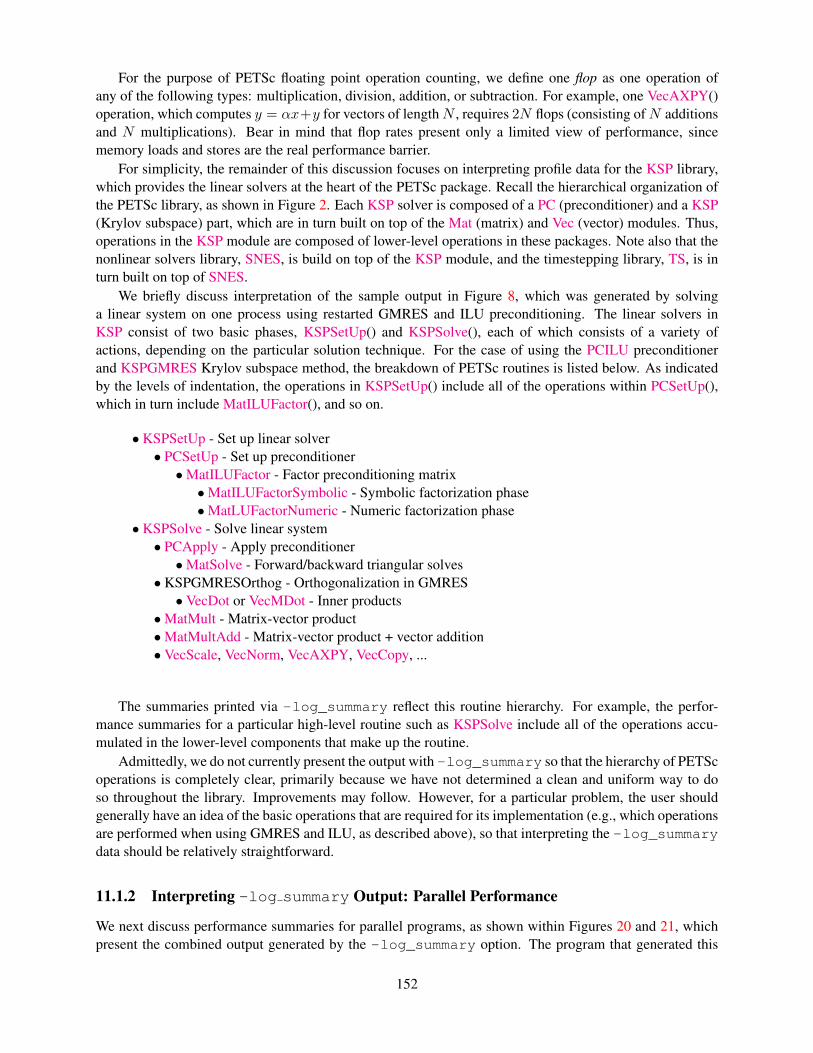
For the purpose of PETSc floating point operation counting, we define one flop as one operation ofany of the following types: multiplication, division, addition, or subtraction. For example, one VecAXPY()operation, which computes y = αx+y for vectors of lengthN , requires 2N flops (consisting ofN additionsand N multiplications). Bear in mind that flop rates present only a limited view of performance, sincememory loads and stores are the real performance barrier.
For simplicity, the remainder of this discussion focuses on interpreting profile data for the KSP library,which provides the linear solvers at the heart of the PETSc package. Recall the hierarchical organization ofthe PETSc library, as shown in Figure 2. Each KSP solver is composed of a PC (preconditioner) and a KSP(Krylov subspace) part, which are in turn built on top of the Mat (matrix) and Vec (vector) modules. Thus,operations in the KSP module are composed of lower-level operations in these packages. Note also that thenonlinear solvers library, SNES, is build on top of the KSP module, and the timestepping library, TS, is inturn built on top of SNES.
We briefly discuss interpretation of the sample output in Figure 8, which was generated by solvinga linear system on one process using restarted GMRES and ILU preconditioning. The linear solvers inKSP consist of two basic phases, KSPSetUp() and KSPSolve(), each of which consists of a variety ofactions, depending on the particular solution technique. For the case of using the PCILU preconditionerand KSPGMRES Krylov subspace method, the breakdown of PETSc routines is listed below. As indicatedby the levels of indentation, the operations in KSPSetUp() include all of the operations within PCSetUp(),which in turn include MatILUFactor(), and so on.
• KSPSetUp - Set up linear solver• PCSetUp - Set up preconditioner•MatILUFactor - Factor preconditioning matrix•MatILUFactorSymbolic - Symbolic factorization phase•MatLUFactorNumeric - Numeric factorization phase
• KSPSolve - Solve linear system• PCApply - Apply preconditioner•MatSolve - Forward/backward triangular solves
• KSPGMRESOrthog - Orthogonalization in GMRES• VecDot or VecMDot - Inner products
•MatMult - Matrix-vector product•MatMultAdd - Matrix-vector product + vector addition• VecScale, VecNorm, VecAXPY, VecCopy, ...
The summaries printed via -log_summary reflect this routine hierarchy. For example, the perfor-mance summaries for a particular high-level routine such as KSPSolve include all of the operations accu-mulated in the lower-level components that make up the routine.
Admittedly, we do not currently present the output with -log_summary so that the hierarchy of PETScoperations is completely clear, primarily because we have not determined a clean and uniform way to doso throughout the library. Improvements may follow. However, for a particular problem, the user shouldgenerally have an idea of the basic operations that are required for its implementation (e.g., which operationsare performed when using GMRES and ILU, as described above), so that interpreting the -log_summarydata should be relatively straightforward.
11.1.2 Interpreting -log summary Output: Parallel Performance
We next discuss performance summaries for parallel programs, as shown within Figures 20 and 21, whichpresent the combined output generated by the -log_summary option. The program that generated this
152
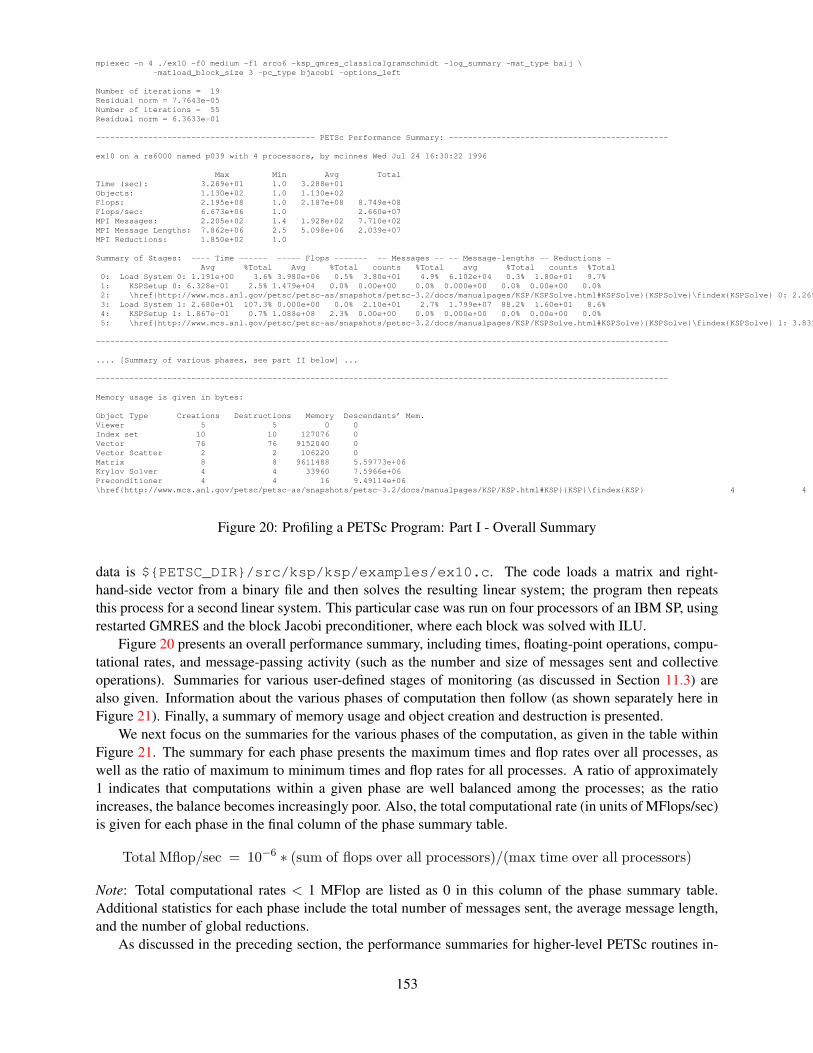
mpiexec -n 4 ./ex10 -f0 medium -f1 arco6 -ksp_gmres_classicalgramschmidt -log_summary -mat_type baij \-matload_block_size 3 -pc_type bjacobi -options_left
Number of iterations = 19Residual norm = 7.7643e-05Number of iterations = 55Residual norm = 6.3633e-01
---------------------------------------------- PETSc Performance Summary: ----------------------------------------------
ex10 on a rs6000 named p039 with 4 processors, by mcinnes Wed Jul 24 16:30:22 1996
Max Min Avg TotalTime (sec): 3.289e+01 1.0 3.288e+01Objects: 1.130e+02 1.0 1.130e+02Flops: 2.195e+08 1.0 2.187e+08 8.749e+08Flops/sec: 6.673e+06 1.0 2.660e+07MPI Messages: 2.205e+02 1.4 1.928e+02 7.710e+02MPI Message Lengths: 7.862e+06 2.5 5.098e+06 2.039e+07MPI Reductions: 1.850e+02 1.0
Summary of Stages: ---- Time ------ ----- Flops ------- -- Messages -- -- Message-lengths -- Reductions -Avg %Total Avg %Total counts %Total avg %Total counts %Total
0: Load System 0: 1.191e+00 3.6% 3.980e+06 0.5% 3.80e+01 4.9% 6.102e+04 0.3% 1.80e+01 9.7%1: KSPSetup 0: 6.328e-01 2.5% 1.479e+04 0.0% 0.00e+00 0.0% 0.000e+00 0.0% 0.00e+00 0.0%2: \href{http://www.mcs.anl.gov/petsc/petsc-as/snapshots/petsc-3.2/docs/manualpages/KSP/KSPSolve.html#KSPSolve}{KSPSolve}\findex{KSPSolve} 0: 2.269e-01 0.9% 1.340e+06 0.0% 1.52e+02 19.7% 9.405e+03 0.0% 3.90e+01 21.1%3: Load System 1: 2.680e+01 107.3% 0.000e+00 0.0% 2.10e+01 2.7% 1.799e+07 88.2% 1.60e+01 8.6%4: KSPSetup 1: 1.867e-01 0.7% 1.088e+08 2.3% 0.00e+00 0.0% 0.000e+00 0.0% 0.00e+00 0.0%5: \href{http://www.mcs.anl.gov/petsc/petsc-as/snapshots/petsc-3.2/docs/manualpages/KSP/KSPSolve.html#KSPSolve}{KSPSolve}\findex{KSPSolve} 1: 3.831e+00 15.3% 2.217e+08 97.1% 5.60e+02 72.6% 2.333e+06 11.4% 1.12e+02 60.5%
------------------------------------------------------------------------------------------------------------------------
.... [Summary of various phases, see part II below] ...
------------------------------------------------------------------------------------------------------------------------
Memory usage is given in bytes:
Object Type Creations Destructions Memory Descendants’ Mem.Viewer 5 5 0 0Index set 10 10 127076 0Vector 76 76 9152040 0Vector Scatter 2 2 106220 0Matrix 8 8 9611488 5.59773e+06Krylov Solver 4 4 33960 7.5966e+06Preconditioner 4 4 16 9.49114e+06\href{http://www.mcs.anl.gov/petsc/petsc-as/snapshots/petsc-3.2/docs/manualpages/KSP/KSP.html#KSP}{KSP}\findex{KSP} 4 4 0 1.71217e+07
Figure 20: Profiling a PETSc Program: Part I - Overall Summary
data is ${PETSC_DIR}/src/ksp/ksp/examples/ex10.c. The code loads a matrix and right-hand-side vector from a binary file and then solves the resulting linear system; the program then repeatsthis process for a second linear system. This particular case was run on four processors of an IBM SP, usingrestarted GMRES and the block Jacobi preconditioner, where each block was solved with ILU.
Figure 20 presents an overall performance summary, including times, floating-point operations, compu-tational rates, and message-passing activity (such as the number and size of messages sent and collectiveoperations). Summaries for various user-defined stages of monitoring (as discussed in Section 11.3) arealso given. Information about the various phases of computation then follow (as shown separately here inFigure 21). Finally, a summary of memory usage and object creation and destruction is presented.
We next focus on the summaries for the various phases of the computation, as given in the table withinFigure 21. The summary for each phase presents the maximum times and flop rates over all processes, aswell as the ratio of maximum to minimum times and flop rates for all processes. A ratio of approximately1 indicates that computations within a given phase are well balanced among the processes; as the ratioincreases, the balance becomes increasingly poor. Also, the total computational rate (in units of MFlops/sec)is given for each phase in the final column of the phase summary table.
Total Mflop/sec = 10−6 ∗ (sum of flops over all processors)/(max time over all processors)
Note: Total computational rates < 1 MFlop are listed as 0 in this column of the phase summary table.Additional statistics for each phase include the total number of messages sent, the average message length,and the number of global reductions.
As discussed in the preceding section, the performance summaries for higher-level PETSc routines in-
153
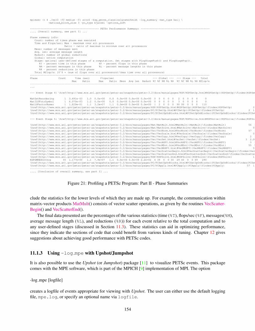
mpiexec -n 4 ./ex10 -f0 medium -f1 arco6 -ksp_gmres_classicalgramschmidt -log_summary -mat_type baij \-matload_block_size 3 -pc_type bjacobi -options_left
---------------------------------------------- PETSc Performance Summary: ----------------------------------------------.... [Overall summary, see part I] ...
Phase summary info:Count: number of times phase was executedTime and Flops/sec: Max - maximum over all processors
Ratio - ratio of maximum to minimum over all processorsMess: number of messages sentAvg. len: average message lengthReduct: number of global reductionsGlobal: entire computationStage: optional user-defined stages of a computation. Set stages with PLogStagePush() and PLogStagePop().
%T - percent time in this phase %F - percent flops in this phase%M - percent messages in this phase %L - percent message lengths in this phase%R - percent reductions in this phase
Total Mflop/s: 10ˆ6 * (sum of flops over all processors)/(max time over all processors)------------------------------------------------------------------------------------------------------------------------Phase Count Time (sec) Flops/sec --- Global --- --- Stage --- Total
Max Ratio Max Ratio Mess Avg len Reduct %T %F %M %L %R %T %F %M %L %R Mflop/s------------------------------------------------------------------------------------------------------------------------...
--- Event Stage 4: \href{http://www.mcs.anl.gov/petsc/petsc-as/snapshots/petsc-3.2/docs/manualpages/KSP/KSPSetUp.html#KSPSetUp}{KSPSetUp}\findex{KSPSetUp} 1
MatGetReordering 1 3.491e-03 1.0 0.0e+00 0.0 0.0e+00 0.0e+00 0.0e+00 0 0 0 0 0 2 0 0 0 0 0MatILUFctrSymbol 1 6.970e-03 1.2 0.0e+00 0.0 0.0e+00 0.0e+00 0.0e+00 0 0 0 0 0 3 0 0 0 0 0MatLUFactorNumer 1 1.829e-01 1.1 3.2e+07 1.1 0.0e+00 0.0e+00 0.0e+00 1 2 0 0 0 90 99 0 0 0 110\href{http://www.mcs.anl.gov/petsc/petsc-as/snapshots/petsc-3.2/docs/manualpages/KSP/KSPSetUp.html#KSPSetUp}{KSPSetUp}\findex{KSPSetUp} 2 1.989e-01 1.1 2.9e+07 1.1 0.0e+00 0.0e+00 0.0e+00 1 2 0 0 0 99 99 0 0 0 102\href{http://www.mcs.anl.gov/petsc/petsc-as/snapshots/petsc-3.2/docs/manualpages/PC/PCSetUp.html#PCSetUp}{PCSetUp}\findex{PCSetUp} 2 1.952e-01 1.1 2.9e+07 1.1 0.0e+00 0.0e+00 0.0e+00 1 2 0 0 0 97 99 0 0 0 104\href{http://www.mcs.anl.gov/petsc/petsc-as/snapshots/petsc-3.2/docs/manualpages/PC/PCSetUpOnBlocks.html#PCSetUpOnBlocks}{PCSetUpOnBlocks}\findex{PCSetUpOnBlocks} 1 1.930e-01 1.1 3.0e+07 1.1 0.0e+00 0.0e+00 0.0e+00 1 2 0 0 0 96 99 0 0 0 105
--- Event Stage 5: \href{http://www.mcs.anl.gov/petsc/petsc-as/snapshots/petsc-3.2/docs/manualpages/KSP/KSPSolve.html#KSPSolve}{KSPSolve}\findex{KSPSolve} 1
\href{http://www.mcs.anl.gov/petsc/petsc-as/snapshots/petsc-3.2/docs/manualpages/Mat/MatMult.html#MatMult}{MatMult}\findex{MatMult} 56 1.199e+00 1.1 5.3e+07 1.0 1.1e+03 4.2e+03 0.0e+00 5 28 99 23 0 30 28 99 99 0 201\href{http://www.mcs.anl.gov/petsc/petsc-as/snapshots/petsc-3.2/docs/manualpages/Mat/MatSolve.html#MatSolve}{MatSolve}\findex{MatSolve} 57 1.263e+00 1.0 4.7e+07 1.0 0.0e+00 0.0e+00 0.0e+00 5 27 0 0 0 33 28 0 0 0 187\href{http://www.mcs.anl.gov/petsc/petsc-as/snapshots/petsc-3.2/docs/manualpages/Vec/VecNorm.html#VecNorm}{VecNorm}\findex{VecNorm} 57 1.528e-01 1.3 2.7e+07 1.3 0.0e+00 0.0e+00 2.3e+02 1 1 0 0 31 3 1 0 0 51 81\href{http://www.mcs.anl.gov/petsc/petsc-as/snapshots/petsc-3.2/docs/manualpages/Vec/VecScale.html#VecScale}{VecScale}\findex{VecScale} 57 3.347e-02 1.0 4.7e+07 1.0 0.0e+00 0.0e+00 0.0e+00 0 1 0 0 0 1 1 0 0 0 184\href{http://www.mcs.anl.gov/petsc/petsc-as/snapshots/petsc-3.2/docs/manualpages/Vec/VecCopy.html#VecCopy}{VecCopy}\findex{VecCopy} 2 1.703e-03 1.1 0.0e+00 0.0 0.0e+00 0.0e+00 0.0e+00 0 0 0 0 0 0 0 0 0 0 0\href{http://www.mcs.anl.gov/petsc/petsc-as/snapshots/petsc-3.2/docs/manualpages/Vec/VecSet.html#VecSet}{VecSet}\findex{VecSet} 3 2.098e-03 1.0 0.0e+00 0.0 0.0e+00 0.0e+00 0.0e+00 0 0 0 0 0 0 0 0 0 0 0\href{http://www.mcs.anl.gov/petsc/petsc-as/snapshots/petsc-3.2/docs/manualpages/Vec/VecAXPY.html#VecAXPY}{VecAXPY}\findex{VecAXPY} 3 3.247e-03 1.1 5.4e+07 1.1 0.0e+00 0.0e+00 0.0e+00 0 0 0 0 0 0 0 0 0 0 200\href{http://www.mcs.anl.gov/petsc/petsc-as/snapshots/petsc-3.2/docs/manualpages/Vec/VecMDot.html#VecMDot}{VecMDot}\findex{VecMDot} 55 5.216e-01 1.2 9.8e+07 1.2 0.0e+00 0.0e+00 2.2e+02 2 20 0 0 30 12 20 0 0 49 327\href{http://www.mcs.anl.gov/petsc/petsc-as/snapshots/petsc-3.2/docs/manualpages/Vec/VecMAXPY.html#VecMAXPY}{VecMAXPY}\findex{VecMAXPY} 57 6.997e-01 1.1 6.9e+07 1.1 0.0e+00 0.0e+00 0.0e+00 3 21 0 0 0 18 21 0 0 0 261\href{http://www.mcs.anl.gov/petsc/petsc-as/snapshots/petsc-3.2/docs/manualpages/Vec/VecScatterBegin.html#VecScatterBegin}{VecScatterBegin}\findex{VecScatterBegin} 56 4.534e-02 1.8 0.0e+00 0.0 1.1e+03 4.2e+03 0.0e+00 0 0 99 23 0 1 0 99 99 0 0\href{http://www.mcs.anl.gov/petsc/petsc-as/snapshots/petsc-3.2/docs/manualpages/Vec/VecScatterEnd.html#VecScatterEnd}{VecScatterEnd}\findex{VecScatterEnd} 56 2.095e-01 1.2 0.0e+00 0.0 0.0e+00 0.0e+00 0.0e+00 1 0 0 0 0 5 0 0 0 0 0\href{http://www.mcs.anl.gov/petsc/petsc-as/snapshots/petsc-3.2/docs/manualpages/KSP/KSPSolve.html#KSPSolve}{KSPSolve}\findex{KSPSolve} 1 3.832e+00 1.0 5.6e+07 1.0 1.1e+03 4.2e+03 4.5e+02 15 97 99 23 61 99 99 99 99 99 222KSPGMRESOrthog 55 1.177e+00 1.1 7.9e+07 1.1 0.0e+00 0.0e+00 2.2e+02 4 39 0 0 30 29 40 0 0 49 290\href{http://www.mcs.anl.gov/petsc/petsc-as/snapshots/petsc-3.2/docs/manualpages/PC/PCSetUpOnBlocks.html#PCSetUpOnBlocks}{PCSetUpOnBlocks}\findex{PCSetUpOnBlocks} 1 1.180e-05 1.1 0.0e+00 0.0 0.0e+00 0.0e+00 0.0e+00 0 0 0 0 0 0 0 0 0 0 0\href{http://www.mcs.anl.gov/petsc/petsc-as/snapshots/petsc-3.2/docs/manualpages/PC/PCApply.html#PCApply}{PCApply}\findex{PCApply} 57 1.267e+00 1.0 4.7e+07 1.0 0.0e+00 0.0e+00 0.0e+00 5 27 0 0 0 33 28 0 0 0 186------------------------------------------------------------------------------------------------------------------------.... [Conclusion of overall summary, see part I] ...
Figure 21: Profiling a PETSc Program: Part II - Phase Summaries
clude the statistics for the lower levels of which they are made up. For example, the communication withinmatrix-vector products MatMult() consists of vector scatter operations, as given by the routines VecScatter-Begin() and VecScatterEnd().
The final data presented are the percentages of the various statistics (time (%T), flops/sec (%F), messages(%M),average message length (%L), and reductions (%R)) for each event relative to the total computation and toany user-defined stages (discussed in Section 11.3). These statistics can aid in optimizing performance,since they indicate the sections of code that could benefit from various kinds of tuning. Chapter 12 givessuggestions about achieving good performance with PETSc codes.
11.1.3 Using -log mpe with Upshot/Jumpshot
It is also possible to use the Upshot (or Jumpshot) package [11] to visualize PETSc events. This packagecomes with the MPE software, which is part of the MPICH [9] implementation of MPI. The option
-log mpe [logfile]
creates a logfile of events appropriate for viewing with Upshot. The user can either use the default loggingfile, mpe.log, or specify an optional name via logfile.
154
By default, not all PETSc events are logged with MPE. For example, since MatSetValues() may be calledthousands of times in a program, by default its calls are not logged with MPE. To activate MPE logging ofa particular event, one should use the command
PetscLogEventMPEActivate(int event);
To deactivate logging of an event for MPE, one should use
PetscLogEventMPEDeactivate(int event);
The event may be either a predefined PETSc event (as listed in the file ${PETSC_DIR}/include/petsclog.h) or one obtained with PetscLogEventRegister() (as described in Section 11.2). These rou-tines may be called as many times as desired in an application program, so that one could restrict MPE eventlogging only to certain code segments.
To see what events are logged by default, the user can view the source code; see the files src/plot/src/plogmpe.c and include/petsclog.h. A simple program and GUI interface to see the eventsthat are predefined and their definition is being developed.
The user can also log MPI events. To do this, simply consider the PETSc application as any MPIapplication, and follow the MPI implementation’s instructions for logging MPI calls. For example, whenusing MPICH, this merely required adding -llmpich to the library list before -lmpich.
11.2 Profiling Application Codes
PETSc automatically logs object creation, times, and floating-point counts for the library routines. Users caneasily supplement this information by monitoring their application codes as well. The basic steps involvedin logging a user-defined portion of code, called an event, are shown in the code fragment below:
#include ”petsclog.h”int USER EVENT;PetscLogEventRegister(”User event name”,0,&USER EVENT);PetscLogEventBegin(USER EVENT,0,0,0,0);/* application code segment to monitor */PetscLogFlops(number of flops for this code segment);PetscLogEventEnd(USER EVENT,0,0,0,0);
One must register the event by calling PetscLogEventRegister(), which assigns a unique integer to iden-tify the event for profiling purposes:
PetscLogEventRegister(const char string[],PetscLogEvent *e);
Here string is a user-defined event name, and color is an optional user-defined event color (for use withUpshot/Nupshot logging); one should see the manual page for details. The argument returned in e shouldthen be passed to the PetscLogEventBegin() and PetscLogEventEnd() routines.
Events are logged by using the pair
PetscLogEventBegin(int event,PetscObject o1,PetscObject o2,PetscObject o3,PetscObject o4);PetscLogEventEnd(int event,PetscObject o1,PetscObject o2,PetscObject o3,PetscObject o4);
155
The four objects are the PETSc objects that are most closely associated with the event. For instance, ina matrix-vector product they would be the matrix and the two vectors. These objects can be omitted byspecifying 0 for o1 - o4. The code between these two routine calls will be automatically timed and loggedas part of the specified event.
The user can log the number of floating-point operations for this segment of code by calling
PetscLogFlops(number of flops for this code segment);
between the calls to PetscLogEventBegin() and PetscLogEventEnd(). This value will automatically be addedto the global flop counter for the entire program.
11.3 Profiling Multiple Sections of Code
By default, the profiling produces a single set of statistics for all code between the PetscInitialize() andPetscFinalize() calls within a program. One can independently monitor up to ten stages of code by switchingamong the various stages with the comands
PetscLogStagePush(PetscLogStage stage);PetscLogStagePop();
where stage is an integer (0-9); see the manual pages for details. The command
PetscLogStageRegister(const char *name,PetscLogStage *stage)
allows one to associate a name with a stage; these names are printed whenever summaries are generatedwith -log_summary or PetscLogView(). The following code fragment uses three profiling stages withinan program.
PetscInitialize(int *argc,char ***args,0,0);/* stage 0 of code here */PetscLogStageRegister(”Stage 0 of Code”,&stagenum0);for(i=0; i¡ntimes; i++) {
PetscLogStageRegister(”Stage 1 of Code”,&stagenum1);PetscLogStagePush(stagenum1);/* stage 1 of code here */PetscLogStagePop();PetscLogStageRegister(”Stage 2 of Code”,&stagenum2);PetscLogStagePush(stagenum2);/* stage 2 of code here */PetscLogStagePop();
} PetscFinalize();
Figures 20 and 21 show output generated by -log_summary for a program that employs severalprofiling stages. In particular, this program is subdivided into six stages: loading a matrix and right-hand-side vector from a binary file, setting up the preconditioner, and solving the linear system; this sequence isthen repeated for a second linear system. For simplicity, Figure 21 contains output only for stages 4 and5 (linear solve of the second system), which comprise the part of this computation of most interest to usin terms of performance monitoring. This code organization (solving a small linear system followed by alarger system) enables generation of more accurate profiling statistics for the second system by overcomingthe often considerable overhead of paging, as discussed in Section 11.8.
156
11.4 Restricting Event Logging
By default, all PETSc operations are logged. To enable or disable the PETSc logging of individual events,one uses the commands
PetscLogEventActivate(int event);PetscLogEventDeactivate(int event);
The event may be either a predefined PETSc event (as listed in the file ${PETSC_DIR}/include/petsclog.h) or one obtained with PetscLogEventRegister() (as described in Section 11.2).
PETSc also provides routines that deactivate (or activate) logging for entire components of the library.Currently, the components that support such logging (de)activation are Mat (matrices), Vec (vectors), KSP(linear solvers, including KSP and PC), and SNES (nonlinear solvers):
PetscLogEventDeactivateClass(MAT CLASSID);PetscLogEventDeactivateClass(KSP CLASSID); /* includes PC and KSP */PetscLogEventDeactivateClass(VEC CLASSID);PetscLogEventDeactivateClass(SNES CLASSID);
and
PetscLogEventActivateClass(MAT CLASSID);PetscLogEventActivateClass(KSP CLASSID); /* includes PC and KSP */PetscLogEventActivateClass(VEC CLASSID);PetscLogEventActivateClass(SNES CLASSID);
Recall that the option -log_all produces extensive profile data, which can be a challenge for PETScViewto handle due to the memory limitations of Tcl/Tk. Thus, one should generally use -log_all when run-ning programs with a relatively small number of events or when disabling some of the events that occurmany times in a code (e.g., VecSetValues(), MatSetValues()).
Section 11.1.3 gives information on the restriction of events in MPE logging.
11.5 Interpreting -log info Output: Informative Messages
Users can activate the printing of verbose information about algorithms, data structures, etc. to the screenby using the option -info or by calling PetscInfoAllow(PETSC_TRUE). Such logging, which is usedthroughout the PETSc libraries, can aid the user in understanding algorithms and tuning program perfor-mance. For example, as discussed in Section 3.1.1, -info activates the printing of information aboutmemory allocation during matrix assembly.
Application programmers can employ this logging as well, by using the routine
PetscInfo(void* obj,char *message,...)
where obj is the PETSc object associated most closely with the logging statement, message. For example,in the line search Newton methods, we use a statement such as
PetscInfo(snes,"Cubically determined step, lambda %g\n",lambda);
One can selectively turn off informative messages about any of the basic PETSc objects (e.g., Mat,SNES) with the command
PetscInfoDeactivateClass(int object classid)
157
where object_classid is one of MAT_CLASSID, SNES_CLASSID, etc. Messages can be reactivatedwith the command
PetscInfoActivateClass(int object classid)
Such deactivation can be useful when one wishes to view information about higher-level PETSc libraries(e.g., TS and SNES) without seeing all lower level data as well (e.g., Mat). One can deactivate events atruntime for matrix and linear solver libraries via -info [no_mat, no_ksp].
11.6 Time
PETSc application programmers can access the wall clock time directly with the command
PetscLogDouble time;PetscGetTime(&time);CHKERRQ(ierr);
which returns the current time in seconds since the epoch, and is commonly implemented with MPI_Wtime.A floating point number is returned in order to express fractions of a second. In addition, as discussed inSection 11.2, PETSc can automatically profile user-defined segments of code.
11.7 Saving Output to a File
All output from PETSc programs (including informative messages, profiling information, and convergencedata) can be saved to a file by using the command line option -history [filename]. If no filename is specified, the output is stored in the file ${HOME}/.petschistory. Note that this optiononly saves output printed with the PetscPrintf() and PetscFPrintf() commands, not the standard printf()and fprintf() statements.
11.8 Accurate Profiling: Overcoming the Overhead of Paging
One factor that often plays a significant role in profiling a code is paging by the operating system. Generally,when running a program only a few pages required to start it are loaded into memory rather than the entireexecutable. When the execution procedes to code segments that are not in memory, a pagefault occurs,prompting the required pages to be loaded from the disk (a very slow process). This activity distorts theresults significantly. (The paging effects are noticeable in the the log files generated by -log_mpe, whichis described in Section 11.1.3.)
To eliminate the effects of paging when profiling the performance of a program, we have found aneffective procedure is to run the exact same code on a small dummy problem before running it on the actualproblem of interest. We thus ensure that all code required by a solver is loaded into memory during solutionof the small problem. When the code procedes to the actual (larger) problem of interest, all required pageshave already been loaded into main memory, so that the performance numbers are not distorted.
When this procedure is used in conjunction with the user-defined stages of profiling described in Sec-tion 11.3, we can focus easily on the problem of interest. For example, we used this technique in theprogram ${PETSC_DIR}/src/ksp/ksp/examples/tutorials/ex10.c to generate the timingswithin Figures 20 and 21. In this case, the profiled code of interest (solving the linear system for the largerproblem) occurs within event stages 4 and 5. Section 11.1.2 provides details about interpreting such profilingdata.
In particular, the macros
158

PetscPreLoadBegin(PetscBool ,char* stagename),PetscPreLoadStage(char *stagename),
and
PetscPreLoadEnd()
can be used to easily convert a regular PETSc program to one that uses preloading. The command lineoptions -preload true and -preload false may be used to turn on and off preloading at run timefor PETSc programs that use these macros.
159

160
Chapter 12
Hints for Performance Tuning
This chapter presents some tips on achieving good performance within PETSc codes. We urge users to readthese hints before evaluating the performance of PETSc application codes.
12.1 Compiler Options
Code configured with --with-debugging=0 faster than that the default debugging version, so we rec-ommend using one of the optimized versions of code when evaluating performance.
12.2 Profiling
Users should not spend time optimizing a code until after having determined where it spends the bulk of itstime on realistically sized problems. As discussed in detail in Chapter 11, the PETSc routines automaticallylog performance data if certain runtime options are specified. We briefly highlight usage of these featuresbelow.
• Run the code with the option -log_summary to print a performance summary for various phasesof the code.
• Run the code with the option -log_mpe [logfilename], which creates a logfile of events suit-able for viewing with Upshot or Nupshot (part of MPICH).
12.3 Aggregation
Performing operations on chunks of data rather than a single element at a time can significantly enhanceperformance.
• Insert several (many) elements of a matrix or vector at once, rather than looping and inserting a singlevalue at a time. In order to access elements in of vector repeatedly, employ VecGetArray() to allowdirect manipulation of the vector elements.
• When possible, use VecMDot() rather than a series of calls to VecDot().
161
12.4 Efficient Memory Allocation
12.4.1 Sparse Matrix Assembly
Since the process of dynamic memory allocation for sparse matrices is inherently very expensive, accu-rate preallocation of memory is crucial for efficient sparse matrix assembly. One should use the matrixcreation routines for particular data structures, such as MatCreateSeqAIJ() and MatCreateMPIAIJ() forcompressed, sparse row formats, instead of the generic MatCreate() routine. For problems with multipledegrees of freedom per node, the block, compressed, sparse row formats, created by MatCreateSeqBAIJ()and MatCreateMPIBAIJ(), can significantly enhance performance. Section 3.1.1 includes extensive detailsand examples regarding preallocation.
12.4.2 Sparse Matrix Factorization
When symbolically factoring an AIJ matrix, PETSc has to guess how much fill there will be. Careful useof the fill parameter in the MatILUInfo structure when calling MatLUFactorSymbolic() or MatILUFac-torSymbolic() can reduce greatly the number of mallocs and copies required, and thus greatly improve theperformance of the factorization. One way to determine a good value for f is to run a program with theoption -info. The symbolic factorization phase will then print information such as
Info:MatILUFactorSymbolic AIJ:Realloc 12 Fill ratio:given 1 needed 2.16423
This indicates that the user should have used a fill estimate factor of about 2.17 (instead of 1) to prevent the12 required mallocs and copies. The command line option
-pc ilu fill 2.17
will cause PETSc to preallocate the correct amount of space for incomplete (ILU) factorization. The corre-sponding option for direct (LU) factorization is -pc_factor_fill <fill_amount\trl{>}.
12.4.3 PetscMalloc() Calls
Users should employ a reasonable number of PetscMalloc() calls in their codes. Hundreds or thousands ofmemory allocations may be appropriate; however, if tens of thousands are being used, then reducing thenumber of PetscMalloc() calls may be warranted. For example, reusing space or allocating large chunks anddividing it into pieces can produce a significant savings in allocation overhead. Section 12.5 gives details.
12.5 Data Structure Reuse
Data structures should be reused whenever possible. For example, if a code often creates new matrices orvectors, there often may be a way to reuse some of them. Very significant performance improvements canbe achieved by reusing matrix data structures with the same nonzero pattern. If a code creates thousands ofmatrix or vector objects, performance will be degraded. For example, when solving a nonlinear problem ortimestepping, reusing the matrices and their nonzero structure for many steps when appropriate can makethe code run significantly faster.
A simple technique for saving work vectors, matrices, etc. is employing a user-defined context. In C andC++ such a context is merely a structure in which various objects can be stashed; in Fortran a user contextcan be an integer array that contains both parameters and pointers to PETSc objects. See ${PETSC_DIR}/snes/examples/tutorials/ex5.c and ${PETSC_DIR}/snes/examples/tutorials/ex5f.F for examples of user-defined application contexts in C and Fortran, respectively.
162
12.6 Numerical Experiments
PETSc users should run a variety of tests. For example, there are a large number of options for the linearand nonlinear equation solvers in PETSc, and different choices can make a very big difference in conver-gence rates and execution times. PETSc employs defaults that are generally reasonable for a wide rangeof problems, but clearly these defaults cannot be best for all cases. Users should experiment with manycombinations to determine what is best for a given problem and customize the solvers accordingly.
• Use the options -snes_view, -ksp_view, etc. (or the routines KSPView(), SNESView(), etc.)to view the options that have been used for a particular solver.
• Run the code with the option -help for a list of the available runtime commands.
• Use the option -info to print details about the solvers’ operation.
• Use the PETSc monitoring discussed in Chapter 11 to evaluate the performance of various numericalmethods.
12.7 Tips for Efficient Use of Linear Solvers
As discussed in Chapter 4, the default linear solvers are
• uniprocess: GMRES(30) with ILU(0) preconditioning
• multiprocess: GMRES(30) with block Jacobi preconditioning, where there is 1 block per process, andeach block is solved with ILU(0)
One should experiment to determine alternatives that may be better for various applications. Recall that onecan specify the KSP methods and preconditioners at runtime via the options:
-ksp type <ksp name> -pc type <pc name>
One can also specify a variety of runtime customizations for the solvers, as discussed throughout the manual.In particular, note that the default restart parameter for GMRES is 30, which may be too small for some
large-scale problems. One can alter this parameter with the option -ksp_gmres_restart <restart> orby calling KSPGMRESSetRestart(). Section 4.3 gives information on setting alternative GMRES orthogo-nalization routines, which may provide much better parallel performance.
12.8 Detecting Memory Allocation Problems
PETSc provides a number of tools to aid in detection of problems with memory allocation, including leaksand use of uninitialized space. We briefly describe these below.
• The PETSc memory allocation (which collects statistics and performs error checking), is employedby default for codes compiled in a debug-mode (configured with --with-debugging=1). PETScmemory allocation can be activated for optimixed-mode (configured with --with-debugging=0)using the option -malloc. The option -malloc=0 forces the use of conventional memory alloca-tion when debugging is enabled. When running timing tests, one should build libraries in optimized-mode.
163
• When the PETSc memory allocation routines are used, the option -malloc_dump will print a listof unfreed memory at the conclusion of a program. If all memory has been freed, only a messagestating the maximum allocated space will be printed. However, if some memory remains unfreed, thisinformation will be printed. Note that the option -malloc_dump merely activates a call to Petsc-MallocDump() during PetscFinalize() the user can also call PetscMallocDump() elsewhere ina program.
• Another useful option for use with PETSc memory allocation routines is -malloc_log, which acti-vates logging of all calls to malloc and reports memory usage, including all Fortran arrays. This optionprovides a more complete picture than -malloc_dump for codes that employ Fortran with hard-wired arrays. The option -malloc_log activates logging by calling PetscMallocSetDumpLog()in PetscInitialize() and then prints the log by calling PetscMallocDumpLog() in PetscFinal-ize(). The user can also call these routines elsewhere in a program. When finer granularity is desired,the user should call PetscMallocGetCurrentUsage() and PetscMallocGetMaximumUsage() for mem-ory allocated by PETSc, or PetscMemoryGetCurrentUsage() and PetscMemoryGetMaximumUsage()for the total memory used by the program. Note that PetscMemorySetGetMaximumUsage() must becalled before PetscMemoryGetMaximumUsage() (typically at the beginning of the program).
12.9 System-Related Problems
The performance of a code can be affected by a variety of factors, including the cache behavior, other userson the machine, etc. Below we briefly describe some common problems and possibilities for overcomingthem.
• Problem too large for physical memory size: When timing a program, one should always leave atleast a ten percent margin between the total memory a process is using and the physical size of themachine’s memory. One way to estimate the amount of memory used by given process is with theUNIX getrusage system routine. Also, the PETSc option -log_summary prints the amountof memory used by the basic PETSc objects, thus providing a lower bound on the memory used.Another useful option is -malloc_log which reports all memory, including any Fortran arrays inan application code.
• Effects of other users: If other users are running jobs on the same physical processor nodes on whicha program is being profiled, the timing results are essentially meaningless.
• Overhead of timing routines on certain machines: On certain machines, even calling the systemclock in order to time routines is slow; this skews all of the flop rates and timing results. The file${PETSC_DIR}/src/benchmarks/PetscTime.c contains a simple test problem that willapproximate the ammount of time required to get the current time in a running program. On goodsystems it will on the order of 1.e-6 seconds or less.
• Problem too large for good cache performance: Certain machines with lower memory bandwidths(slow memory access) attempt to compensate by having a very large cache. Thus, if a significantportion of an application fits within the cache, the program will achieve very good performance; if thecode is too large, the performance can degrade markedly. To analyze whether this situation affects aparticular code, one can try plotting the total flop rate as a function of problem size. If the flop ratedecreases rapidly at some point, then the problem may likely be too large for the cache size.
• Inconsistent timings: Inconsistent timings are likely due to other users on the machine, thrashing(using more virtual memory than available physical memory), or paging in of the initial executable.
164

Section 11.8 provides information on overcoming paging overhead when profiling a code. We havefound on all systems that if you follow all the advise above your timings will be consistent within avariation of less than five percent.
165

166
Chapter 13
Other PETSc Features
13.1 PETSc on a process subset
Users who wish to employ PETSc routines on only a subset of processes within a larger parallel job, orwho wish to use a “master” process to coordinate the work of “slave” PETSc processes, should specify analternative communicator for PETSC_COMM_WORLD by calling
PetscSetCommWorld(MPI Comm comm);
before calling PetscInitialize(), but, obviously, after calling MPI_Init(). PetscSetCommWorld() can becalled at most once per process. Most users will never need to use the routine PetscSetCommWorld().
13.2 Runtime Options
Allowing the user to modify parameters and options easily at runtime is very desirable for many applications.PETSc provides a simple mechanism to enable such customization. To print a list of available options for agiven program, simply specify the option -help (or -h) at runtime, e.g.,
mpiexec -n 1 ./ex1 -help
Note that all runtime options correspond to particular PETSc routines that can be explicitly called fromwithin a program to set compile-time defaults. For many applications it is natural to use a combination ofcompile-time and runtime choices. For example, when solving a linear system, one could explicitly specifyuse of the Krylov subspace technique BiCGStab by calling
KSPSetType(ksp,KSPBCGS);
One could then override this choice at runtime with the option
-ksp type tfqmr
to select the Transpose-Free QMR algorithm. (See Chapter 4 for details.)The remainder of this section discusses details of runtime options.
13.2.1 The Options Database
Each PETSc process maintains a database of option names and values (stored as text strings). This databaseis generated with the command PETScInitialize(), which is listed below in its C/C++ and Fortran variants,respectively:
167
PetscInitialize(int *argc,char ***args,const char *file,const char *help);call PetscInitialize(character file,integer ierr)
The arguments argc and args (in the C/C++ version only) are the addresses of usual command linearguments, while the file is a name of a file that can contain additional options. By default this file iscalled .petscrc in the user’s home directory. The user can also specify options via the environmentalvariable PETSC_OPTIONS. The options are processed in the following order:
• file
• environmental variable
• command line
Thus, the command line options supersede the environmental variable options, which in turn supersede theoptions file.
The file format for specifying options is
-optionname possible value-anotheroptionname possible value...
All of the option names must begin with a dash (-) and have no intervening spaces. Note that the optionvalues cannot have intervening spaces either, and tab characters cannot be used between the option namesand values. The user can employ any naming convention. For uniformity throughout PETSc, we employ theformat -package_option (for instance, -ksp_type and -mat_view_info).
Users can specify an alias for any option name (to avoid typing the sometimes lengthy default name) byadding an alias to the .petscrc file in the format
alias -newname -oldname
For example,
alias -kspt -ksp typealias -sd -start in debugger
Comments can be placed in the .petscrc file by using one of the following symbols in the first column of aline: #, %, or !.
13.2.2 User-Defined PetscOptions
Any subroutine in a PETSc program can add entries to the database with the command
PetscOptionsSetValue(char *name,char *value);
though this is rarely done. To locate options in the database, one should use the commands
PetscOptionsHasName(char *pre,char *name,PetscBool *flg);PetscOptionsGetInt(char *pre,char *name,int *value,PetscBool *flg);PetscOptionsGetReal(char *pre,char *name,double *value,PetscBool *flg);PetscOptionsGetString(char *pre,char *name,char *value,int maxlen,PetscBool *flg);PetscOptionsGetStringArray(char *pre,char *name,char **values,int *maxlen,PetscBool *flg);PetscOptionsGetIntArray(char *pre,char *name,int *value,int *nmax,PetscBool *flg);PetscOptionsGetRealArray(char *pre,char *name,double *value, int *nmax,PetscBool *flg);
168
All of these routines set flg=PETSC_TRUE if the corresponding option was found, flg=PETSC_FALSEif it was not found. The optional argument pre indicates that the true name of the option is the given name(with the dash “-” removed) prepended by the prefix pre. Usually pre should be set to PETSC NULL(or PETSC_NULL_CHARACTER for Fortran); its purpose is to allow someone to rename all the optionsin a package without knowing the names of the individual options. For example, when using block Jacobipreconditioning, the KSP and PC methods used on the individual blocks can be controlled via the options-sub_ksp_type and -sub_pc_type.
13.2.3 Keeping Track of Options
One useful means of keeping track of user-specified runtime options is use of -options_table, whichprints to stdout during PetscFinalize() a table of all runtime options that the user has specified.A related option is -options_left, which prints the options table and indicates any options that havenot been requested upon a call to PetscFinalize(). This feature is useful to check whether an option has beenactivated for a particular PETSc object (such as a solver or matrix format), or whether an option name mayhave been accidentally misspelled.
13.3 Viewers: Looking at PETSc Objects
PETSc employs a consistent scheme for examining, printing, and saving objects through commands of theform
XXXView(XXX obj,PetscViewer viewer);
Here obj is any PETSc object of type XXX, where XXX is Mat, Vec, SNES, etc. There are several predefinedviewers:
• Passing in a zero for the viewer causes the object to be printed to the screen; this is most useful whenviewing an object in a debugger.
• PETSC VIEWER STDOUT SELF and PETSC VIEWER STDOUT WORLD cause the object to beprinted to the screen.
• PETSC VIEWER DRAW SELF PETSC VIEWER DRAW WORLD causes the object to be drawnin a default X window.
• Passing in a viewer obtained by PetscViewerDrawOpen() causes the object to be displayed graphically.
• To save an object to a file in ASCII format, the user creates the viewer object with the commandPetscViewerASCIIOpen(MPI_Comm comm, char* file, PetscViewer *viewer). Thisobject is analogous to PETSC VIEWER STDOUT SELF (for a communicator of MPI_COMM_SELF) and PETSC VIEWER STDOUT WORLD (for a parallel communicator).
• To save an object to a file in binary format, the user creates the viewer object with the commandPetscViewerBinaryOpen(MPI_Comm comm,char* file,PetscViewerBinaryType type, PetscViewer *viewer).Details of binary I/O are discussed below.
• Vector and matrix objects can be passed to a running MATLAB process with a viewer created by
PetscViewerSocketOpen(MPI Comm comm,char *machine,int port,PetscViewer *viewer).
169
On the MATLAB side, one must first run v = sreader(int port) and then A = PetscBinaryRead(v) to obtain the matrix or vector. Once all objects have been received, the port can beclosed from the MATLAB end with close(v). On the PETSc side, one should destroy the viewerobject with PetscViewerDestroy(). The corresponding MATLAB mex files are located in${PETSC_DIR}/src/sys/viewer/impls/socket/matlab.
The user can control the format of ASCII printed objects with viewers created by PetscViewerASCI-IOpen() by calling
PetscViewerSetFormat(PetscViewer viewer,int format);
Possible formats include PETSC_VIEWER_DEFAULT, PETSC_VIEWER_ASCII_MATLAB, and PETSC_VIEWER_ASCII_IMPL. The implementation-specific format, PETSC_VIEWER_ASCII_IMPL, dis-plays the object in the most natural way for a particular implementation.
The routines
PetscViewerPushFormat(PetscViewer viewer,int format);PetscViewerPopFormat(PetscViewer viewer);
allow one to temporarily change the format of a viewer.As discussed above, one can output PETSc objects in binary format by first opening a binary viewer
with PetscViewerBinaryOpen() and then using MatView(), VecView(), etc. The corresponding routines forinput of a binary object have the form XXXLoad(). In particular, matrix and vector binary input is handledby the following routines:
MatLoad(PetscViewer viewer,MatType outtype,Mat *newmat);VecLoad(PetscViewer viewer,VecType outtype,Vec *newvec);
These routines generate parallel matrices and vectors if the viewer’s communicator has more than one pro-cess. The particular matrix and vector formats are determined from the options database; see the manualpages for details.
One can provide additional information about matrix data for matrices stored on disk by providing anoptional file matrixfilename.info, where matrixfilename is the name of the file containing thematrix. The format of the optional file is the same as the .petscrc file and can (currently) contain thefollowing:
-matload block size <bs>
The block size indicates the size of blocks to use if the matrix is read into a block oriented data structure (forexample, MATMPIBAIJ). The diagonal information s1,s2,s3,... indicates which (block) diagonalsin the matrix have nonzero values.
13.4 Debugging
PETSc programs may be debugged using one of the two options below.
• -start_in_debugger [noxterm,dbx,xxgdb] [-display name] - start all processesin debugger
• -on_error_attach_debugger [noxterm,dbx,xxgdb] [-display name] - start de-bugger only on encountering an error
170
Note that, in general, debugging MPI programs cannot be done in the usual manner of starting the program-ming in the debugger (because then it cannot set up the MPI communication and remote processes).
By default the GNU debugger gdb is used when -start_in_debugger or -on_error_attach_debugger is specified. To employ either xxgdb or the common UNIX debugger dbx, one uses commandline options as indicated above. On HP-UX machines the debugger xdb should be used instead of dbx; onRS/6000 machines the xldb debugger is supported as well. By default, the debugger will be started in a newxterm (to enable running separate debuggers on each process), unless the option noxterm is used. In orderto handle the MPI startup phase, the debugger command “cont” should be used to continue execution of theprogram within the debugger. Rerunning the program through the debugger requires terminating the firstjob and restarting the processor(s); the usual “run” option in the debugger will not correctly handle the MPIstartup and should not be used. Not all debuggers work on all machines, so the user may have to experimentto find one that works correctly.
You can select a subset of the processes to be debugged (the rest just run without the debugger) with theoption
-debugger nodes node1,node2,...
where you simply list the nodes you want the debugger to run with.
13.5 Error Handling
Errors are handled through the routine PetscError(). This routine checks a stack of error handlers and callsthe one on the top. If the stack is empty, it selects PetscTraceBackErrorHandler(), which tries to print atraceback. A new error handler can be put on the stack with
PetscPushErrorHandler(PetscErrorCode (*HandlerFunction)(int line,char *dir,char *file,char *message,int number,void*),void *HandlerContext)
The arguments to HandlerFunction() are the line number where the error occurred, the file in whichthe error was detected, the corresponding directory, the error message, the error integer, and the HandlerContext. The routine
PetscPopErrorHandler()
removes the last error handler and discards it.PETSc provides two additional error handlers besides PetscTraceBackErrorHandler():
PetscAbortErrorHandler()PetscAttachErrorHandler()
The function PetscAbortErrorHandler() calls abort on encountering an error, while PetscAttachErrorHan-dler() attaches a debugger to the running process if an error is detected. At runtime, these error handlerscan be set with the options -on_error_abort or -on_error_attach_debugger [noxterm,dbx, xxgdb, xldb] [-display DISPLAY].
All PETSc calls can be traced (useful for determining where a program is hanging without running inthe debugger) with the option
-log trace [filename]
where filename is optional. By default the traces are printed to the screen. This can also be set with thecommand PetscLogTraceBegin(FILE*).
It is also possible to trap signals by using the command
171
PetscPushSignalHandler( PetscErrorCode (*Handler)(int,void *),void *ctx);
The default handler PetscDefaultSignalHandler() calls PetscError() and then terminates. In general, a signalin PETSc indicates a catastrophic failure. Any error hander that the user provides should try to clean up onlybefore exiting. By default all PETSc programs use the default signal handler, although the user can turn thisoff at runtime with the option -no_signal_handler .
There is a separate signal handler for floating-point exceptions. The option -fp_trap turns on thefloating-point trap at runtime, and the routine
PetscSetFPTrap(int flag);
can be used in-line. A flag of PETSC_FP_TRAP_ON indicates that floating-point exceptions should betrapped, while a value of PETSC_FP_TRAP_OFF (the default) indicates that they should be ignored. Notethat on certain machines, in particular the IBM RS/6000, trapping is very expensive.
A small set of macros is used to make the error handling lightweight. These macros are used throughoutthe PETSc libraries and can be employed by the application programmer as well. When an error is firstdetected, one should set it by calling
SETERRQ(MPI Comm comm,PetscErrorCode flag,,char *message);
The user should check the return codes for all PETSc routines (and possibly user-defined routines as well)with
ierr = PetscRoutine(...);CHKERRQ(PetscErrorCode ierr);
Likewise, all memory allocations should be checked with
ierr = PetscMalloc(n*sizeof(double),&ptr);CHKERRQ(ierr);
If this procedure is followed throughout all of the user’s libraries and codes, any error will by default generatea clean traceback of the location of the error.
Note that the macro __FUNCT__ is used to keep track of routine names during error tracebacks. Usersneed not worry about this macro in their application codes; however, users can take advantage of this featureif desired by setting this macro before each user-defined routine that may call SETERRQ(), CHKERRQ().A simple example of usage is given below.
#undef FUNCT#define FUNCT ”MyRoutine1”int MyRoutine1() {/* code here */return 0;}
13.6 Incremental Debugging
When developing large codes, one is often in the position of having a correctly (or at least believed to becorrectly) running code; making a change to the code then changes the results for some unknown reason.Often even determining the precise point at which the old and new codes diverge is a major pain. In othercases, a code generates different results when run on different numbers of processes, although in exactarithmetic the same answer is expected. (Of course, this assumes that exactly the same solver and parametersare used in the two cases.)
PETSc provides some support for determining exactly where in the code the computations lead to differ-ent results. First, compile both programs with different names. Next, start running both programs as a single
172
MPI job. This procedure is dependent on the particular MPI implementation being used. For example, whenusing MPICH on workstations, procgroup files can be used to specify the processors on which the job is tobe run. Thus, to run two programs, old and new, each on two processors, one should create the procgroupfile with the following contents:
local 0workstation1 1 /home/bsmith/oldworkstation2 1 /home/bsmith/newworkstation3 1 /home/bsmith/new
(Of course, workstation1, etc. can be the same machine.) Then, one can execute the command
mpiexec -p4pg <procgroup filemame> old -compare <tolerance> [options]
Note that the same runtime options must be used for the two programs. The first time an inner productor norm detects an inconsistency larger than <tolerance>, PETSc will generate an error. The usualruntime options -start_in_debugger and -on_error_attach_debugger may be used. Theuser can also place the commands
PetscCompareDouble()PetscCompareScalar()PetscCompareInt()
in portions of the application code to check for consistency between the two versions.
13.7 Complex Numbers
PETSc supports the use of complex numbers in application programs written in C, C++, and Fortran. To doso, we employ either the C99 complex type or the C++ versions of the PETSc libraries in which the basic“scalar” datatype, given in PETSc codes by PetscScalar, is defined as complex (or complex<double>for machines using templated complex class libraries). To work with complex numbers, the user shouldrun ./configure with the additional option --with-scalar-type=complex. The file ${PETSC_DIR}/src/docs/website/documentation/installation.html provides detailed instructionsfor installing PETSc. You can use --with-clanguage=c (the default) to use the C99 complex numbersor --with-clanguage=c++ to use the C++ complex type.
We recommend using optimized Fortran kernels for some key numerical routines with complex numbers(such as matrix-vector products, vector norms, etc.) instead of the default C/C++ routines. This can bedone with the ./configure option --with-fortran-kernels=generic. This implementationexploits the maturity of Fortran compilers while retaining the identical user interface. For example, onrs6000 machines, the base single-node performance when using the Fortran kernels is 4-5 times faster thanthe default C++ code.
Recall that each variant of the PETSc libraries is stored in a different directory, given by
${PETSC_DIR}/lib/${PETSC_ARCH},
according to the architecture.. Thus, the libraries for complex numbers are maintained separately fromthose for real numbers. When using any of the complex numbers versions of PETSc, all vector and matrixelements are treated as complex, even if their imaginary components are zero. Of course, one can elect touse only the real parts of the complex numbers when using the complex versions of the PETSc libraries;however, when working only with real numbers in a code, one should use a version of PETSc for realnumbers for best efficiency.
173
The program ${PETSC_DIR}/src/ksp/ksp/examples/tutorials/ex11.c solves a linearsystem with a complex coefficient matrix. Its Fortran counterpart is ${PETSC_DIR}/src/ksp/ksp/examples/tutorials/ex11f.F.
13.8 Emacs Users
If users develop application codes using Emacs (which we highly recommend), the etags feature canbe used to search PETSc files quickly and efficiently. To use this feature, one should first check if thefile, ${PETSC_DIR}/TAGS exists. If this file is not present, it should be generated by running makealletags from the PETSc home directory. Once the file exists, from Emacs the user should issue thecommand
M-x visit-tags-table
where “M” denotes the Emacs Meta key, and enter the name of the TAGS file. Then the command “M-.” willcause Emacs to find the file and line number where a desired PETSc function is defined. Any string in anyof the PETSc files can be found with the command “M-x tags-search”. To find repeated occurrences,one can simply use “M-,” to find the next occurrence.
An alternative which provides reverse lookups (e.g. find all call sites for a given function) and is some-what more amenable to managing many projects is GNU Global, available from http://www.gnu.org/s/global/. Tags for PETSc and all external packages can be generated by running the command
find $PETSC_DIR/{include,src,tutorials,$PETSC_ARCH/include} any/other/paths \-regex ’.*\.\(cc\|hh\|cpp\|C\|hpp\|c\|h\|cu\)$’ \| grep -v ftn-auto | gtags -f -
from your home directory or wherever you keep source code. If you are making large changes, it is usefulto either set this up to run as a cron job or to make a convenient alias so that refreshing is easy. Then add thefollowing to ˜/.emacs to enable gtags and replace the plain etags bindings.
(when (require ’gtags)(global-set-key "\C-cf" ’gtags-find-file)(global-set-key "\M-." ’gtags-find-tag)(define-key gtags-mode-map (kbd "C-c r") ’gtags-find-rtag))
(add-hook ’c-mode-common-hook’(lambda () (gtags-mode t))) ; Or add to existing hook
13.9 Vi and Vim Users
If users develop application codes using Vi or Vim the tags feature can be used to search PETSc filesquickly and efficiently. To use this feature, one should first check if the file, ${PETSC_DIR}/CTAGSexists. If this file is not present, it should be generated by running make alletags from the PETSc homedirectory. Once the file exists, from Vi/Vim the user should issue the command
:set tags=CTAGS
from the PETSC_DIR directory and enter the name of the CTAGS file. Then the command “tag function-name” will cause Vi/Vim to find the file and line number where a desired PETSc function is defined. See,for example, http://www.yolinux.com/TUTORIALS/LinuxTutorialAdvanced vi.html for additional Vi/Vimoptions that allow searches etc. It is also possible to use GNU Global with Vim, see the description forEmacs above.
174
13.10 Eclipse Users
If you are interested in developing code that uses PETSc from Eclipse or developing PETSc in Eclipseand have knowledge of how to do indexing and build libraries in Eclipse please contact us at [email protected].
To allow an Eclipse code to compile with the PETSc include files and link with the PETSc librariessomeone has suggested To do this, click on your managed C project with the right sided mouse button,select
Properties -¿ C/C++ Build -¿ SettingsThen you get a new window with on the right hand side the various setting options.Select Includes, and add the required PETSc paths. In my case I have added
${PETSC_DIR}/include${PETSC_DIR}/${PETSC_ARCH}/include
Then select ”Libraries” under the header Linker and you should set the Library search path:
${PETSC_DIR}/${PETSC_ARCH}/lib
and then the libraries, in my case:
m, petsc, stdc++, mpichxx, mpich, lapack, blas, gfortran, dl, rt,gcc_s, pthread, X11
To make PETSc an Eclipse package
• Install the Mecurial plugin for Eclipse and then import the PETSc repository to Eclipse.
• elected New-¿Convert to C/C++ project and selected shared library. After this point you can performsearchs in the code.
A PETSc user has provided the following steps to build an Eclipse index for PETSc that can be usedwith their own code without compiling PETSc source into their project.
• In the user project source directory, create a symlink to the petsc/src directory.
• Refresh the project explorer in Eclipse, so the new symlink is followed.
• Right-click on the project in the project explorer, and choose ”Index -¿ Rebuild”. The index shouldnow be build.
• Right-click on the PETSc symlink in the project explorer, and choose ”Exclude from build...” to makesure Eclipse does not try to compile PETSc with the project.
13.11 Qt Creator
Qt Creator is developed as a part of Qt SDK for cross-platform GUI programming using C++ and thus hasexcellent support for application developing using C/C++. This information was provided by MohammadMirzadeh.
1. Qt Creator supports automated and cross-platform qmake and Cmake build systems. What thismeans, is that, starting from a handful set of options, Qt Creator is able to generate makefiles that areused to compile and run your application package on Linux, Windows and Mac systems.
2. Qt Creator makes the task of linking PETSc library to your application package easy.
3. Qt Creator has visual debugger and supports both GNU’s GDB and Microsoft’s CDB (on Windows).
175
4. Qt Creator (as of version 2.3) has interface to memory profiling softwares such as valgrind.
5. Qt Creator has built-in auto-completion and function look-up. This feature of editor, makes it possiblefor the user to easily browse inside huge packages like PETSc and easily find relevant functions andobjects.
6. Qt Creator has inline error/warning messages. This feature of the editor greatly reduces programmingbugs by informing the user of potential error/warning as the code is being written and even before thecompile step.
7. Qt Creator is an excellent environment for doing GUI programming using Qt framework. This meansyou can easily generate a nice GUI for you application package as well!
Qt Creator is a part of Qt SDK, currently being developed by Nokia Inc. It is available under GPL v3,LGPL v2 and a commercial license and may be obtained, either as a part of Qt SDK or as an stand-alonesoftware, via http://qt.nokia.com/downloads/.
How to create a project?
Upon installation, all you really need to do to port your software package to Qt Creator is to build a .profile. A .pro file is simply a configuration file that tells Qt Creator about all build/compile options andlocations of source file. One may start with a blank .pro file and fill in the configuration options as needed:
TARGET = n a m e o f y o u r a p p
APP DIR = / home / p a t h / t o / your / appPETSC DIR = / home / p a t h / t o / your / p e t s cPETSC ARCH = l i n u x−gnu−cxx−debugPETSC BINS = $$PETSC DIR / $$PETSC ARCH / b i n
INCLUDEPATH += $$APP DIR / i n c l u d e \$$PETSC DIR / i n c l u d e \$$PETSC DIR / $$PETSC ARCH / i n c l u d e
LIBS += −L / p a t h / t o / p e t s c / l i b s − l a l l n e e d e d p e t s c l i b s
QMAKE CC = $$PETSC BINS /\ h r e f { h t t p : / / www. mcs . a n l . gov / p e t s c / p e t s c−as / s n a p s h o t s / p e t s c −3 .2 / docs / h t t p : / / www. mcs . a n l . gov / mpi /www/www1/ mpicc . h tml # mpicc }{mpicc }\ f i n d e x {mpicc}QMAKE CXX = $$PETSC BINS / mpicxx
QMAKE CFLAGS += −O3QMAKE CXXFLAGS += −O3QMAKE LFLAGS += −O3
SOURCES += \$$APP DIR / s r c / s o u r c e 1 . cpp \$$APP DIR / s r c / s o u r c e 2 . cpp \$$APP DIR / s r c / main . cppHEADERS += \$$APP DIR / s r c / s o u r c e 1 . h \
176
$$APP DIR / s r c / s o u r c e 2 . hOTHER FILES += \$$APP DIR / s r c / s o m e f i l e . cpp \$$APP DIR / d i r / a n o t h e r f i l e . xyz
In this example, there are different keywords used. These include:
• TARGET: This defines the name of your application executable. You can choose it however you like.
• INCLUDEPATH: This is used in the compile time to point to all the needed include files. Essentially itis used as a -I $$INCLUDEPATH flag for the compiler. This should include all your application-specific header files and those related to PETSc which may be found via make getincludedirs.
• LIBS: This defines all needed external libraries to link with your application. To get PETSc’s linkinglibraries do make getlinklibs.
• QMAKE CC and QMAKE CXX: These define which C/C++ compilers to choose for your application.
• QMAKE CFLAGS, QMAKE CXXFLAGS and QMAKE LFLAGS: These set the corresponding compileand linking flags.
• SOURCES: This sets all the source files that need to be compiled.
• HEADERS: This sets all the header files that are needed for your application. Note that since headerfiles are merely included in the source files, they are not compiled. As a result this is an optional flagand is simply included to allow users to easily access the header files in their application (or evenPETSc header files).
• OTHER FILES: This can be used to virtually include any other file (source, header or any otherextension) just as a way to make accessing to auxiliary files easier. They could be anything from atext file to a PETSc source file. Note that none of the source files placed here are compiled.
Note that there are many more options available that one can feed into the .pro file. For more informa-tion, one should follow http://doc.qt.nokia.com/latest/qmake-variable-reference.html. Once the .pro file is generated, the user can simply open it via Qt Creator. Upon opening, generallyone has the option to create two different build options, debug and release, and switch between the two easilyat any time. For more information on how to use the Qt Creator interface, and other more advanced aspects ofthis IDE, one may refer to http://doc.qt.nokia.com/qtcreator-snapshot/index.html
13.12 Developers Studio Users
In the projects subdirectory of PETSc are several Developers Studio projects that use PETSc.
13.13 XCode Users (The Apple GUI Development System
Please let us know how you have set things up at [email protected].
13.14 Parallel Communication
When used in a message-passing environment, all communication within PETSc is done through MPI, themessage-passing interface standard [14]. Any file that includes petscsys.h (or any other PETSc includefile), can freely use any MPI routine.
177
13.15 Graphics
PETSc graphics library is not intended to compete with high-quality graphics packages. Instead, it is in-tended to be easy to use interactively with PETSc programs. We urge users to generate their publication-quality graphics using a professional graphics package. If a user wants to hook certain packages in PETSc,he or she should send a message to [email protected], and we will see whether it is reasonable totry to provide direct interfaces.
13.15.1 Windows as PetscViewers
For drawing predefined PETSc objects such as matrices and vectors, one must first create a viewer using thecommand
PetscViewerDrawOpen(MPI Comm comm,char *display,char *title,int x,int y,int w,int h,PetscViewer *viewer);
This viewer may be passed to any of the XXXView() routines. To draw into the viewer, one must obtainthe Draw object with the command
PetscViewerDrawGetDraw(PetscViewer viewer,PetscDraw *draw);
Then one can call any of the PetscDrawXXX commands on the draw object. If one obtains the drawobject in this manner, one does not call the PetscDrawOpenX() command discussed below.
Predefined viewers, PETSC VIEWER DRAW WORLD and PETSC VIEWER DRAW SELF, may beused at any time. Their initial use will cause the appropriate window to be created.
By default, PETSc drawing tools employ a private colormap, which remedies the problem of poor colorchoices for contour plots due to an external program’s mangling of the colormap (e.g, Netscape tends todo this). Unfortunately, this causes flashing of colors as the mouse is moved between the PETSc windowsand other windows. Alternatively, a shared colormap can be used via the option -draw_x_shared_colormap.
13.15.2 Simple PetscDrawing
One can open a window that is not associated with a viewer directly under the X11 Window System withthe command
PetscDrawOpenX(MPI Comm comm,char *display,char *title,int x,int y,int w,int h,PetscDraw *win);
All drawing routines are done relative to the windows coordinate system and viewport. By default the draw-ing coordinates are from (0,0) to (1,1), where (0,0) indicates the lower left corner of the window.The application program can change the window coordinates with the command
PetscDrawSetCoordinates(PetscDraw win,double xl,double yl,double xr,double yr);
By default, graphics will be drawn in the entire window. To restrict the drawing to a portion of the window,one may use the command
PetscDrawSetViewPort(PetscDraw win,double xl,double yl,double xr,double yr);
These arguments, which indicate the fraction of the window in which the drawing should be done, mustsatisfy 0 ≤ xl ≤ xr ≤ 1 and 0 ≤ yl ≤ yr ≤ 1.
To draw a line, one uses the command
178
PetscDrawLine(PetscDraw win,double xl,double yl,double xr,double yr,int cl);
The argument cl indicates the color (which is an integer between 0 and 255) of the line. A list of predefinedcolors may be found in include/petscdraw.h and includes PETSC_DRAW_BLACK, PETSC_DRAW_RED, PETSC_DRAW_BLUE etc.
To ensure that all graphics actually have been displayed, one should use the command
PetscDrawFlush(PetscDraw win);
When displaying by using double buffering, which is set with the command
PetscDrawSetDoubleBuffer(PetscDraw win);
all processes must call
PetscDrawSynchronizedFlush(PetscDraw win);
in order to swap the buffers. From the options database one may use -draw_pause n, which causes thePETSc application to pause n seconds at each PetscDrawPause(). A time of -1 indicates that the applicationshould pause until receiving mouse input from the user.
Text can be drawn with either of the two commands
PetscDrawString(PetscDraw win,double x,double y,int color,char *text);PetscDrawStringVertical(PetscDraw win,double x,double y,int color,char *text);
The user can set the text font size or determine it with the commands
PetscDrawStringSetSize(PetscDraw win,double width,double height);PetscDrawStringGetSize(PetscDraw win,double *width,double *height);
13.15.3 Line Graphs
PETSc includes a set of routines for manipulating simple two-dimensional graphs. These routines, whichbegin with PetscDrawAxisDraw(), are usually not used directly by the application programmer. Instead, theprogrammer employs the line graph routines to draw simple line graphs. As shown in the program, withinFigure 22, line graphs are created with the command
PetscDrawLGCreate(PetscDraw win,int ncurves,PetscDrawLG *ctx);
The argument ncurves indicates how many curves are to be drawn. Points can be added to each of thecurves with the command
PetscDrawLGAddPoint(PetscDrawLG ctx,double *x,double *y);
The arguments x and y are arrays containing the next point value for each curve. Several points for eachcurve may be added with
PetscDrawLGAddPoints(PetscDrawLG ctx,int n,double **x,double **y);
The line graph is drawn (or redrawn) with the command
PetscDrawLGDraw(PetscDrawLG ctx);
A line graph that is no longer needed can be destroyed with the command
PetscDrawLGDestroy(PetscDrawLG *ctx);
179
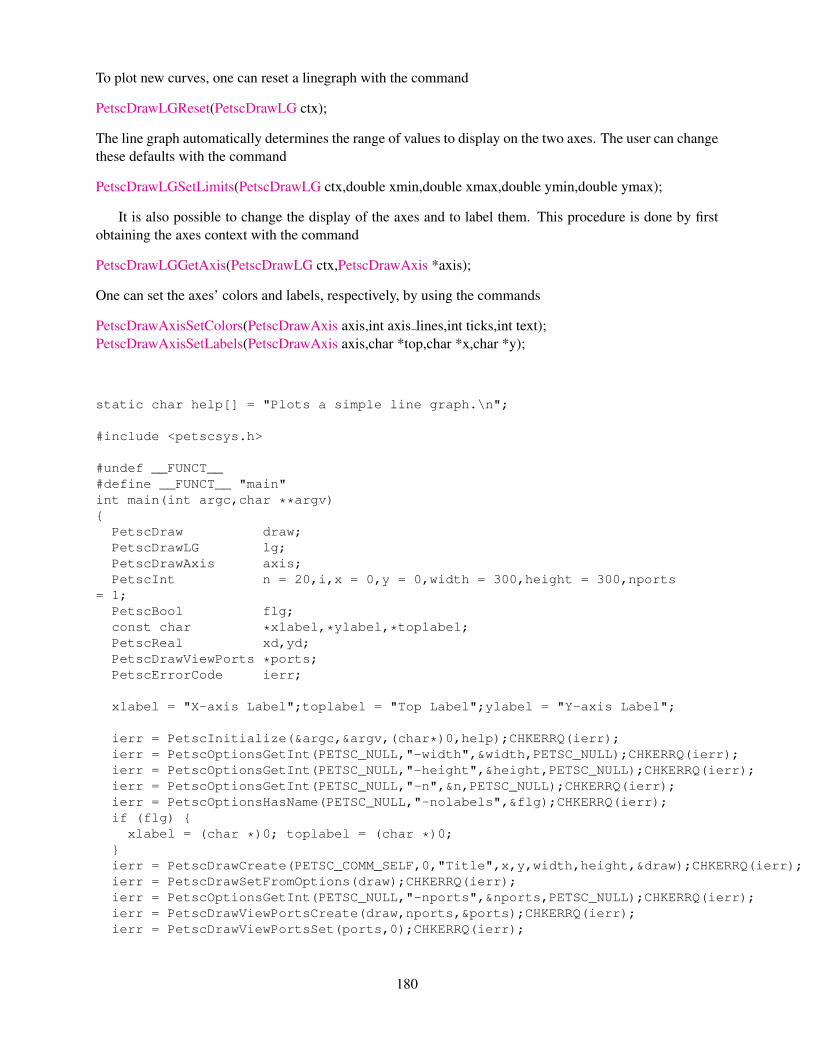
To plot new curves, one can reset a linegraph with the command
PetscDrawLGReset(PetscDrawLG ctx);
The line graph automatically determines the range of values to display on the two axes. The user can changethese defaults with the command
PetscDrawLGSetLimits(PetscDrawLG ctx,double xmin,double xmax,double ymin,double ymax);
It is also possible to change the display of the axes and to label them. This procedure is done by firstobtaining the axes context with the command
PetscDrawLGGetAxis(PetscDrawLG ctx,PetscDrawAxis *axis);
One can set the axes’ colors and labels, respectively, by using the commands
PetscDrawAxisSetColors(PetscDrawAxis axis,int axis lines,int ticks,int text);PetscDrawAxisSetLabels(PetscDrawAxis axis,char *top,char *x,char *y);
static char help[] = "Plots a simple line graph.\n";
#include <petscsys.h>
#undef __FUNCT__#define __FUNCT__ "main"int main(int argc,char **argv){
PetscDraw draw;PetscDrawLG lg;PetscDrawAxis axis;PetscInt n = 20,i,x = 0,y = 0,width = 300,height = 300,nports
= 1;PetscBool flg;const char *xlabel,*ylabel,*toplabel;PetscReal xd,yd;PetscDrawViewPorts *ports;PetscErrorCode ierr;
xlabel = "X-axis Label";toplabel = "Top Label";ylabel = "Y-axis Label";
ierr = PetscInitialize(&argc,&argv,(char*)0,help);CHKERRQ(ierr);ierr = PetscOptionsGetInt(PETSC_NULL,"-width",&width,PETSC_NULL);CHKERRQ(ierr);ierr = PetscOptionsGetInt(PETSC_NULL,"-height",&height,PETSC_NULL);CHKERRQ(ierr);ierr = PetscOptionsGetInt(PETSC_NULL,"-n",&n,PETSC_NULL);CHKERRQ(ierr);ierr = PetscOptionsHasName(PETSC_NULL,"-nolabels",&flg);CHKERRQ(ierr);if (flg) {
xlabel = (char *)0; toplabel = (char *)0;}ierr = PetscDrawCreate(PETSC_COMM_SELF,0,"Title",x,y,width,height,&draw);CHKERRQ(ierr);ierr = PetscDrawSetFromOptions(draw);CHKERRQ(ierr);ierr = PetscOptionsGetInt(PETSC_NULL,"-nports",&nports,PETSC_NULL);CHKERRQ(ierr);ierr = PetscDrawViewPortsCreate(draw,nports,&ports);CHKERRQ(ierr);ierr = PetscDrawViewPortsSet(ports,0);CHKERRQ(ierr);
180
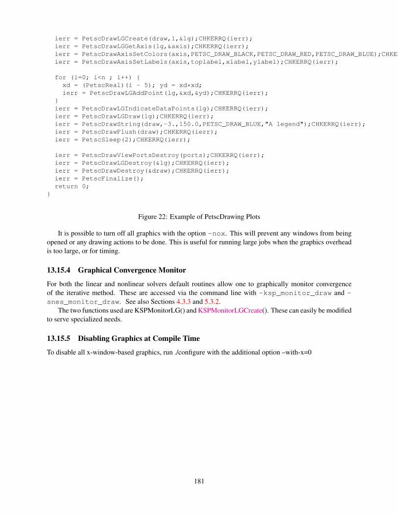
ierr = PetscDrawLGCreate(draw,1,&lg);CHKERRQ(ierr);ierr = PetscDrawLGGetAxis(lg,&axis);CHKERRQ(ierr);ierr = PetscDrawAxisSetColors(axis,PETSC_DRAW_BLACK,PETSC_DRAW_RED,PETSC_DRAW_BLUE);CHKERRQ(ierr);ierr = PetscDrawAxisSetLabels(axis,toplabel,xlabel,ylabel);CHKERRQ(ierr);
for (i=0; i<n ; i++) {xd = (PetscReal)(i - 5); yd = xd*xd;ierr = PetscDrawLGAddPoint(lg,&xd,&yd);CHKERRQ(ierr);
}ierr = PetscDrawLGIndicateDataPoints(lg);CHKERRQ(ierr);ierr = PetscDrawLGDraw(lg);CHKERRQ(ierr);ierr = PetscDrawString(draw,-3.,150.0,PETSC_DRAW_BLUE,"A legend");CHKERRQ(ierr);ierr = PetscDrawFlush(draw);CHKERRQ(ierr);ierr = PetscSleep(2);CHKERRQ(ierr);
ierr = PetscDrawViewPortsDestroy(ports);CHKERRQ(ierr);ierr = PetscDrawLGDestroy(&lg);CHKERRQ(ierr);ierr = PetscDrawDestroy(&draw);CHKERRQ(ierr);ierr = PetscFinalize();return 0;
}
Figure 22: Example of PetscDrawing Plots
It is possible to turn off all graphics with the option -nox. This will prevent any windows from beingopened or any drawing actions to be done. This is useful for running large jobs when the graphics overheadis too large, or for timing.
13.15.4 Graphical Convergence Monitor
For both the linear and nonlinear solvers default routines allow one to graphically monitor convergenceof the iterative method. These are accessed via the command line with -ksp_monitor_draw and -snes_monitor_draw. See also Sections 4.3.3 and 5.3.2.
The two functions used are KSPMonitorLG() and KSPMonitorLGCreate(). These can easily be modifiedto serve specialized needs.
13.15.5 Disabling Graphics at Compile Time
To disable all x-window-based graphics, run ./configure with the additional option –with-x=0
181

182
Chapter 14
Makefiles
This chapter describes the design of the PETSc makefiles, which are the key to managing our code portabilityacross a wide variety of UNIX and Windows systems.
14.1 Our Makefile System
To make a program named ex1, one may use the command
make PETSC ARCH=arch ex1
which will compile the example and automatically link the appropriate libraries. The architecture, arch, isone of solaris, rs6000, IRIX, hpux, etc. Note that when using command line options with make(as illustrated above), one must not place spaces on either side of the “=” signs. The variable PETSC_ARCHcan also be set as environmental variables. Although PETSc is written in C, it can be compiled with a C++compiler. For many C++ users this may be the preferred route. To compile with the C++ compiler, oneshould use the ./configure option --with-clanguage=c++.
14.1.1 Makefile Commands
The directory ${PETSC_DIR}/conf contains virtually all makefile commands and customizations to en-able portability across different architectures. Most makefile commands for maintaining the PETSc systemare defined in the file ${PETSC_DIR}/conf. These commands, which process all appropriate files withinthe directory of execution, include
• lib - Updates the PETSc libraries based on the source code in the directory.
• libfast - Updates the libraries faster. Since libfast recompiles all source files in the directoryat once, rather than individually, this command saves time when many files must be compiled.
• clean - Removes garbage files.
The tree command enables the user to execute a particular action within a directory and all of its sub-directories. The action is specified by ACTION=[action], where action is one of the basic commandslisted above. For example, if the command
make ACTION=lib tree
were executed from the directory ${PETSC_DIR}/src/ksp/ksp, the debugging library for all Krylovsubspace solvers would be built.
183
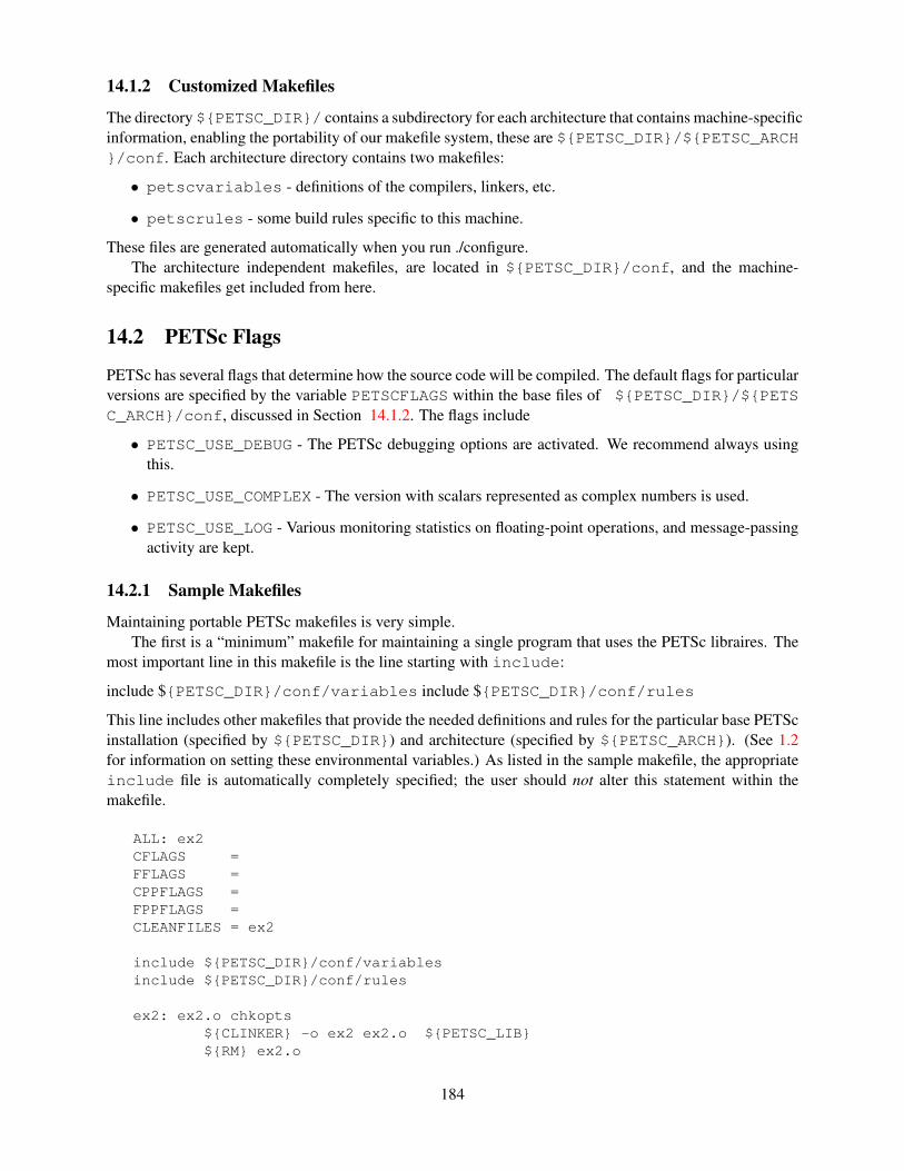
14.1.2 Customized Makefiles
The directory ${PETSC_DIR}/ contains a subdirectory for each architecture that contains machine-specificinformation, enabling the portability of our makefile system, these are ${PETSC_DIR}/${PETSC_ARCH}/conf. Each architecture directory contains two makefiles:
• petscvariables - definitions of the compilers, linkers, etc.
• petscrules - some build rules specific to this machine.
These files are generated automatically when you run ./configure.The architecture independent makefiles, are located in ${PETSC_DIR}/conf, and the machine-
specific makefiles get included from here.
14.2 PETSc Flags
PETSc has several flags that determine how the source code will be compiled. The default flags for particularversions are specified by the variable PETSCFLAGS within the base files of ${PETSC_DIR}/${PETSC_ARCH}/conf, discussed in Section 14.1.2. The flags include
• PETSC_USE_DEBUG - The PETSc debugging options are activated. We recommend always usingthis.
• PETSC_USE_COMPLEX - The version with scalars represented as complex numbers is used.
• PETSC_USE_LOG - Various monitoring statistics on floating-point operations, and message-passingactivity are kept.
14.2.1 Sample Makefiles
Maintaining portable PETSc makefiles is very simple.The first is a “minimum” makefile for maintaining a single program that uses the PETSc libraires. The
most important line in this makefile is the line starting with include:
include ${PETSC_DIR}/conf/variables include ${PETSC_DIR}/conf/rules
This line includes other makefiles that provide the needed definitions and rules for the particular base PETScinstallation (specified by ${PETSC_DIR}) and architecture (specified by ${PETSC_ARCH}). (See 1.2for information on setting these environmental variables.) As listed in the sample makefile, the appropriateinclude file is automatically completely specified; the user should not alter this statement within themakefile.
ALL: ex2CFLAGS =FFLAGS =CPPFLAGS =FPPFLAGS =CLEANFILES = ex2
include ${PETSC_DIR}/conf/variablesinclude ${PETSC_DIR}/conf/rules
ex2: ex2.o chkopts${CLINKER} -o ex2 ex2.o ${PETSC_LIB}${RM} ex2.o
184
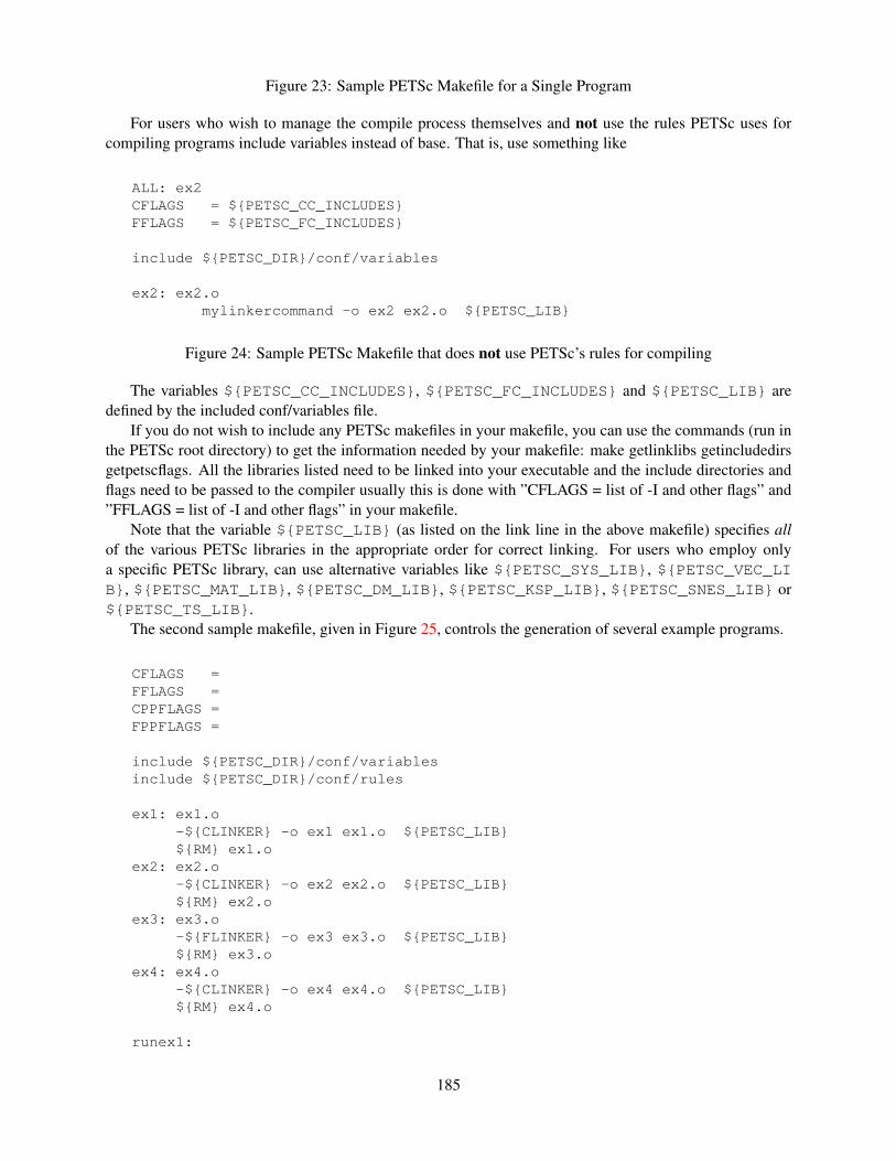
Figure 23: Sample PETSc Makefile for a Single Program
For users who wish to manage the compile process themselves and not use the rules PETSc uses forcompiling programs include variables instead of base. That is, use something like
ALL: ex2CFLAGS = ${PETSC_CC_INCLUDES}FFLAGS = ${PETSC_FC_INCLUDES}
include ${PETSC_DIR}/conf/variables
ex2: ex2.omylinkercommand -o ex2 ex2.o ${PETSC_LIB}
Figure 24: Sample PETSc Makefile that does not use PETSc’s rules for compiling
The variables ${PETSC_CC_INCLUDES}, ${PETSC_FC_INCLUDES} and ${PETSC_LIB} aredefined by the included conf/variables file.
If you do not wish to include any PETSc makefiles in your makefile, you can use the commands (run inthe PETSc root directory) to get the information needed by your makefile: make getlinklibs getincludedirsgetpetscflags. All the libraries listed need to be linked into your executable and the include directories andflags need to be passed to the compiler usually this is done with ”CFLAGS = list of -I and other flags” and”FFLAGS = list of -I and other flags” in your makefile.
Note that the variable ${PETSC_LIB} (as listed on the link line in the above makefile) specifies allof the various PETSc libraries in the appropriate order for correct linking. For users who employ onlya specific PETSc library, can use alternative variables like ${PETSC_SYS_LIB}, ${PETSC_VEC_LIB}, ${PETSC_MAT_LIB}, ${PETSC_DM_LIB}, ${PETSC_KSP_LIB}, ${PETSC_SNES_LIB} or${PETSC_TS_LIB}.
The second sample makefile, given in Figure 25, controls the generation of several example programs.
CFLAGS =FFLAGS =CPPFLAGS =FPPFLAGS =
include ${PETSC_DIR}/conf/variablesinclude ${PETSC_DIR}/conf/rules
ex1: ex1.o-${CLINKER} -o ex1 ex1.o ${PETSC_LIB}${RM} ex1.o
ex2: ex2.o-${CLINKER} -o ex2 ex2.o ${PETSC_LIB}${RM} ex2.o
ex3: ex3.o-${FLINKER} -o ex3 ex3.o ${PETSC_LIB}${RM} ex3.o
ex4: ex4.o-${CLINKER} -o ex4 ex4.o ${PETSC_LIB}${RM} ex4.o
runex1:
185
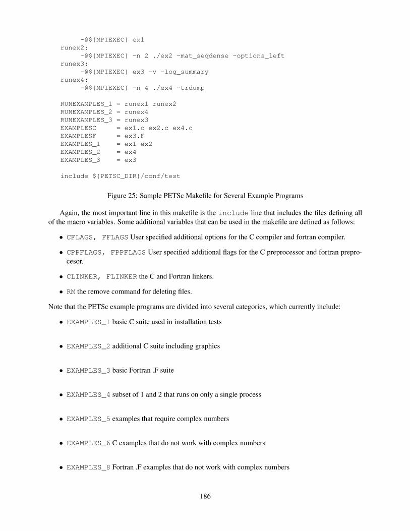
-@${MPIEXEC} ex1runex2:
-@${MPIEXEC} -n 2 ./ex2 -mat_seqdense -options_leftrunex3:
-@${MPIEXEC} ex3 -v -log_summaryrunex4:
-@${MPIEXEC} -n 4 ./ex4 -trdump
RUNEXAMPLES_1 = runex1 runex2RUNEXAMPLES_2 = runex4RUNEXAMPLES_3 = runex3EXAMPLESC = ex1.c ex2.c ex4.cEXAMPLESF = ex3.FEXAMPLES_1 = ex1 ex2EXAMPLES_2 = ex4EXAMPLES_3 = ex3
include ${PETSC_DIR}/conf/test
Figure 25: Sample PETSc Makefile for Several Example Programs
Again, the most important line in this makefile is the include line that includes the files defining allof the macro variables. Some additional variables that can be used in the makefile are defined as follows:
• CFLAGS, FFLAGS User specified additional options for the C compiler and fortran compiler.
• CPPFLAGS, FPPFLAGS User specified additional flags for the C preprocessor and fortran prepro-cesor.
• CLINKER, FLINKER the C and Fortran linkers.
• RM the remove command for deleting files.
Note that the PETSc example programs are divided into several categories, which currently include:
• EXAMPLES_1 basic C suite used in installation tests
• EXAMPLES_2 additional C suite including graphics
• EXAMPLES_3 basic Fortran .F suite
• EXAMPLES_4 subset of 1 and 2 that runs on only a single process
• EXAMPLES_5 examples that require complex numbers
• EXAMPLES_6 C examples that do not work with complex numbers
• EXAMPLES_8 Fortran .F examples that do not work with complex numbers
186
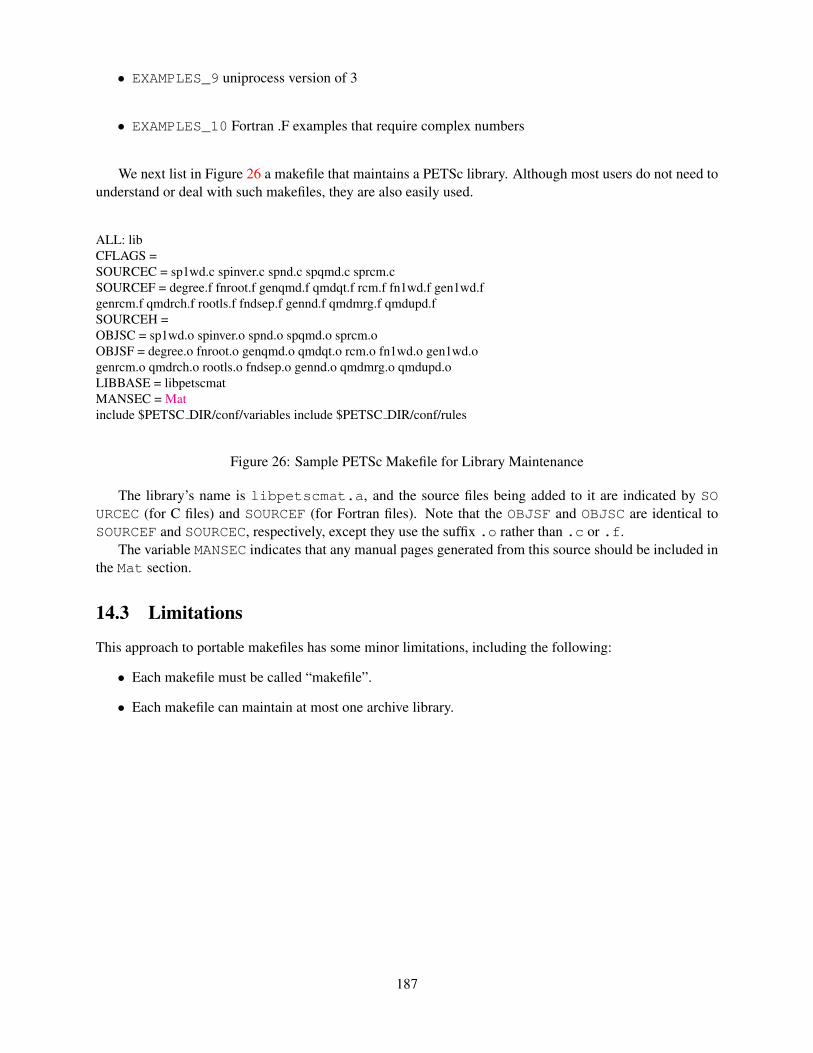
• EXAMPLES_9 uniprocess version of 3
• EXAMPLES_10 Fortran .F examples that require complex numbers
We next list in Figure 26 a makefile that maintains a PETSc library. Although most users do not need tounderstand or deal with such makefiles, they are also easily used.
ALL: libCFLAGS =SOURCEC = sp1wd.c spinver.c spnd.c spqmd.c sprcm.cSOURCEF = degree.f fnroot.f genqmd.f qmdqt.f rcm.f fn1wd.f gen1wd.fgenrcm.f qmdrch.f rootls.f fndsep.f gennd.f qmdmrg.f qmdupd.fSOURCEH =OBJSC = sp1wd.o spinver.o spnd.o spqmd.o sprcm.oOBJSF = degree.o fnroot.o genqmd.o qmdqt.o rcm.o fn1wd.o gen1wd.ogenrcm.o qmdrch.o rootls.o fndsep.o gennd.o qmdmrg.o qmdupd.oLIBBASE = libpetscmatMANSEC = Matinclude $PETSC DIR/conf/variables include $PETSC DIR/conf/rules
Figure 26: Sample PETSc Makefile for Library Maintenance
The library’s name is libpetscmat.a, and the source files being added to it are indicated by SOURCEC (for C files) and SOURCEF (for Fortran files). Note that the OBJSF and OBJSC are identical toSOURCEF and SOURCEC, respectively, except they use the suffix .o rather than .c or .f.
The variable MANSEC indicates that any manual pages generated from this source should be included inthe Mat section.
14.3 Limitations
This approach to portable makefiles has some minor limitations, including the following:
• Each makefile must be called “makefile”.
• Each makefile can maintain at most one archive library.
187

188
Chapter 15
Unimportant and Advanced Features ofMatrices and Solvers
This chapter introduces additional features of the PETSc matrices and solvers. Since most PETSc usersshould not need to use these features, we recommend skipping this chapter during an initial reading.
15.1 Extracting Submatrices
One can extract a (parallel) submatrix from a given (parallel) using
MatGetSubMatrix(Mat A,IS rows,IS cols,MatReuse call,Mat *B);
This extracts the rows and columns of the matrix A into B. If call is MAT_INITIAL_MATRIX it willcreate the matrix B. If call is MAT_REUSE_MATRIX it will reuse the B created with a previous call.
15.2 Matrix Factorization
Normally, PETSc users will access the matrix solvers through the KSP interface, as discussed in Chapter 4,but the underlying factorization and triangular solve routines are also directly accessible to the user.
The LU and Cholesky matrix factorizations are split into two or three stages depending on the user’sneeds. The first stage is to calculate an ordering for the matrix. The ordering generally is done to reduce fillin a sparse factorization; it does not make much sense for a dense matrix.
MatGetOrdering(Mat matrix,MatOrderingType type,IS* rowperm,IS* colperm);
The currently available alternatives for the ordering type are
• MATORDERINGNATURAL - Natural
• MATORDERINGND - Nested Dissection
• MATORDERING1WD - One-way Dissection
• MATORDERINGRCM - Reverse Cuthill-McKee
• MATORDERINGQMD - Quotient Minimum Degree
189
These orderings can also be set through the options database.Certain matrix formats may support only a subset of these; more options may be added. Check the
manual pages for up-to-date information. All of these orderings are symmetric at the moment; orderingroutines that are not symmetric may be added. Currently we support orderings only for sequential matrices.
Users can add their own ordering routines by providing a function with the calling sequence
int reorder(Mat A,MatOrderingType type,IS* rowperm,IS* colperm);
Here A is the matrix for which we wish to generate a new ordering, type may be ignored and rowpermand colperm are the row and column permutations generated by the ordering routine. The user registersthe ordering routine with the command
MatOrderingRegisterDynamic(MatOrderingType inname,char *path,char *sname,PetscErrorCode (*reorder)(Mat,MatOrderingType,IS*,IS*)));
The input argument inname is a string of the user’s choice, iname is either an ordering defined inpetscmat.h or a users string, to indicate one is introducing a new ordering, while the output See thecode in src/mat/impls/order/sorder.c and other files in that directory for examples on how thereordering routines may be written.
Once the reordering routine has been registered, it can be selected for use at runtime with the commandline option -pc_factor_mat_ordering_type sname. If reordering directly, the user should providethe name as the second input argument of MatGetOrdering().
The following routines perform complete, in-place, symbolic, and numerical factorizations for symmet-ric and nonsymmetric matrices, respectively:
MatCholeskyFactor(Mat matrix,IS permutation,const MatFactorInfo *info);MatLUFactor(Mat matrix,IS rowpermutation,IS columnpermutation,const MatFactorInfo *info);
The argument info->fill > 1 is the predicted fill expected in the factored matrix, as a ratio of theoriginal fill. For example, info->fill=2.0 would indicate that one expects the factored matrix to havetwice as many nonzeros as the original.
For sparse matrices it is very unlikely that the factorization is actually done in-place. More likely, newspace is allocated for the factored matrix and the old space deallocated, but to the user it appears in-placebecause the factored matrix replaces the unfactored matrix.
The two factorization stages can also be performed separately, by using the out-of-place mode, first oneobtains that matrix object that will hold the factor
MatGetFactor(Mat matrix,const MatSolverPackage package,MatFactorType ftype,Mat *factor);
and then performs the factorization
MatCholeskyFactorSymbolic(Mat factor,Mat matrix,IS perm,const MatFactorInfo *info);MatLUFactorSymbolic(Mat factor,Mat matrix,IS rowperm,IS colperm,const MatFactorInfo *info);MatCholeskyFactorNumeric(Mat factor,Mat matrix,const MatFactorInfo);MatLUFactorNumeric(Mat factor,Mat matrix,const MatFactorInfo *info);
In this case, the contents of the matrix result is undefined between the symbolic and numeric factorizationstages. It is possible to reuse the symbolic factorization. For the second and succeeding factorizations, onesimply calls the numerical factorization with a new input matrix and the same factored result matrix. Itis essential that the new input matrix have exactly the same nonzero structure as the original factored matrix.(The numerical factorization merely overwrites the numerical values in the factored matrix and does notdisturb the symbolic portion, thus enabling reuse of the symbolic phase.) In general, calling XXXFactorS
190
ymbolic with a dense matrix will do nothing except allocate the new matrix; the XXXFactorNumericroutines will do all of the work.
Why provide the plain XXXfactor routines when one could simply call the two-stage routines? Theanswer is that if one desires in-place factorization of a sparse matrix, the intermediate stage between thesymbolic and numeric phases cannot be stored in a result matrix, and it does not make sense to store theintermediate values inside the original matrix that is being transformed. We originally made the combinedfactor routines do either in-place or out-of-place factorization, but then decided that this approach was notneeded and could easily lead to confusion.
We do not currently support sparse matrix factorization with pivoting for numerical stability. This isbecause trying to both reduce fill and do pivoting can become quite complicated. Instead, we provide a poorstepchild substitute. After one has obtained a reordering, with MatGetOrdering(Mat A,MatOrdering type,IS*row,IS *col) one may call
MatReorderForNonzeroDiagonal(Mat A,double tol,IS row, IS col);
which will try to reorder the columns to ensure that no values along the diagonal are smaller than tol ina absolute value. If small values are detected and corrected for, a nonsymmetric permutation of the rowsand columns will result. This is not guaranteed to work, but may help if one was simply unlucky in theoriginal ordering. When using the KSP solver interface the option -pc_factor_nonzeros_along_diagonal <tol> may be used. Here, tol is an optional tolerance to decide if a value is nonzero; bydefault it is 1.e− 10.
Once a matrix has been factored, it is natural to solve linear systems. The following four routines enablethis process:
MatSolve(Mat A,Vec x, Vec y);MatSolveTranspose(Mat A, Vec x, Vec y);MatSolveAdd(Mat A,Vec x, Vec y, Vec w);MatSolveTransposeAdd(Mat A, Vec x, Vec y, Vec w);
matrix A of these routines must have been obtained from a factorization routine; otherwise, an error will begenerated. In general, the user should use the KSP solvers introduced in the next chapter rather than usingthese factorization and solve routines directly.
15.3 Unimportant Details of KSP
Again, virtually all users should use KSP through the KSP interface and, thus, will not need to know thedetails that follow.
It is possible to generate a Krylov subspace context with the command
KSPCreate(MPI Comm comm,KSP *kps);
Before using the Krylov context, one must set the matrix-vector multiplication routine and the preconditionerwith the commands
PCSetOperators(PC pc,Mat mat,Mat pmat,MatStructure flag);KSPSetPC(KSP ksp,PC pc);
In addition, the KSP solver must be initialized with
KSPSetUp(KSP ksp);
Solving a linear system is done with the command
191
KSPSolve(KSP ksp,Vec b,Vec x);
Finally, the KSP context should be destroyed with
KSPDestroy(KSP *ksp);
It may seem strange to put the matrix in the preconditioner rather than directly in the KSP; this decisionwas the result of much agonizing. The reason is that for SSOR with Eisenstat’s trick, and certain otherpreconditioners, the preconditioner has to change the matrix-vector multiply. This procedure could not bedone cleanly if the matrix were stashed in the KSP context that PC cannot access.
Any preconditioner can supply not only the preconditioner, but also a routine that essentially performsa complete Richardson step. The reason for this is mainly SOR. To use SOR in the Richardson framework,that is,
un+1 = un +B(f −Aun),
is much more expensive than just updating the values. With this addition it is reasonable to state that all ouriterative methods are obtained by combining a preconditioner from the PC package with a Krylov methodfrom the KSP package. This strategy makes things much simpler conceptually, so (we hope) clean codewill result. Note: We had this idea already implicitly in older versions of KSP, but, for instance, just doingGauss-Seidel with Richardson in old KSP was much more expensive than it had to be. With PETSc thisshould not be a problem.
15.4 Unimportant Details of PC
Most users will obtain their preconditioner contexts from the KSP context with the command KSPGetPC().It is possible to create, manipulate, and destroy PC contexts directly, although this capability should rarelybe needed. To create a PC context, one uses the command
PCCreate(MPI Comm comm,PC *pc);
The routine
PCSetType(PC pc,PCType method);
sets the preconditioner method to be used. The routine
PCSetOperators(PC pc,Mat mat,Mat pmat,MatStructure flag);
set the matrices that are to be used with the preconditioner. The routine
PCGetOperators(PC pc,Mat *mat,Mat *pmat,MatStructure *flag);
returns the values set with PCSetOperators().The preconditioners in PETSc can be used in several ways. The two most basic routines simply apply
the preconditioner or its transpose and are given, respectively, by
PCApply(PC pc,Vec x,Vec y);PCApplyTranspose(PC pc,Vec x,Vec y);
In particular, for a preconditioner matrix, B, that has been set via PCSetOperators(pc,A,B,flag), the routinePCApply(pc,x,y) computes y = B−1x by solving the linear system By = x with the specified precondi-tioner method.
Additional preconditioner routines are
192

PCApplyBAorAB(PC pc,PCSide right,Vec x,Vec y,Vec work,int its);PCApplyBAorABTranspose(PC pc,PCSide right,Vec x,Vec y,Vec work,int its);PCApplyRichardson(PC pc,Vec x,Vec y,Vec work,PetscReal rtol,PetscReal atol, PetscReal dtol,PetscInt
maxits,PetscBool zeroguess,PetscInt *its,PCRichardsonConvergedReason*);
The first two routines apply the action of the matrix followed by the preconditioner or the preconditionerfollowed by the matrix depending on whether the right is PC_LEFT or PC_RIGHT. The final routineapplies its iterations of Richardson’s method. The last three routines are provided to improve efficiencyfor certain Krylov subspace methods.
A PC context that is no longer needed can be destroyed with the command
PCDestroy(PC *pc);
193

194
Chapter 16
Unstructured Grids in PETSc
This chapter introduces the DMMesh subclass of DM, which allows the user to handle unstructured gridsusing the generic DM interface for hierarchy and multi-physics. The underlying implementation is writtenin C++, and thus requires PETSc to be build using –with-clanguage=c++. More advanced features will alsorequire direct C++ access in the user code, however much can be done using only the C/F77/F90 interface.
16.1 Sections: Vectors on Unstructured Grids
16.1.1 Defining Sections
The sequence for setting up any Section is the following:
1. Specify the chart
2. Specify the fiber dimensions
3. Allocate
4. Specify the values
We will expand on each item in turn.First, you specify the chart, which is the domain for the Section. For any Section retrieved from the
Mesh, for instance using MeshGetSectionReal(), this is done automatically.Second, you determine sizes for both values and constraints at the same time:
f o r ( l oop ove r p o i n t s ) {s e c t i o n−>s e t F i b e r D i m e n s i o n ( p , dof ) ;
}f o r ( l oop ove r boundary p o i n t s ) {
s e c t i o n−>s e t C o n s t r a i n t D i m e n s i o n ( p , n u m C o n s t r a i n t s ) ;}
Third, we allocate storage for this section
s e c t i o n−>a l l o c a t e P o i n t ( )
which also creates storage for the boundary conditions.Now you can input values and constraints whenever you want
195
f o r ( l oop ove r p o i n t s ) {s e c t i o n−>u p d a t e P o i n t ( p , v a l u e s ) ;
}f o r ( l oop ove r boundary p o i n t s ) {
/∗ Here we c o n s t r a i n t h e x and y v a l u e s ∗ /i n t d o f s [ 2 ] = {0 , 1} ;
s e c t i o n−>s e t C o n s t r a i n t D o f ( p , d o f s ) ;}
Notice that the input to setConstraintDofs() are the local dofs which are fixed.
16.1.2 Updating Values
There are many kinds of update*() functions since users want different ways of setting values. As anexample, we will take a point p with 3 degrees of freedom (u,v,w), and we constrain v, so the fiber dimensionis 3, the constraint dimension is 1, and the constraint dof is [1]. Now, the simplest update is
section-¿updatePoint(p, [a, b, c])which will set the values ’a’ and ’c’, ignoring ’b’ since it is constrained. The function updateAddPoint()
does the same thing but adds the values. We have a similar functionsection-¿updateFreePoint(p, [a, c])which updates the unconstrained values, and only takes those values as input. If you want to update
constrained values, you could usesection-¿updatePointBC(p, [b])which updates the values of constrained unknowns, and takes only the constraint values. You could also
usesection-¿updatePointBCFull(p, [a, b, c])which takes all the values, but only updates the constraint ’b’. Finally,section-¿updatePointAll(p, [a, b, c])takes the all values and updates all of them, ignoring constraints.
196
Index
-compare, 173-dmmg grid sequence, 124-draw pause, 179-fp trap, 22, 172-h, 22, 167-help, 167-history, 158-info, 60, 62, 151, 157-ksp atol, 75-ksp compute eigenvalues, 77-ksp compute eigenvalues explicitly, 77-ksp divtol, 75-ksp gmres cgs refinement type, 73-ksp gmres classicalgramschmidt, 73-ksp gmres modifiedgramschmidt, 73-ksp gmres restart, 73-ksp max it, 75-ksp monitor, 76, 123-ksp monitor cancel, 76-ksp monitor draw, 76, 181-ksp monitor short, 77-ksp monitor singular value, 76-ksp monitor true residual, 76-ksp pc side, 74-ksp plot eigenvalues, 77-ksp plot eigenvalues explicitly, 77-ksp richardson scale, 73-ksp rtol, 75-ksp type, 73-log mpe, 154, 161-log summary, 151, 152, 161-log trace, 151, 171-malloc, 163-malloc dump, 163-malloc log, 164-mat aij oneindex, 59-mat coloring, 112-mat fd coloring err, 112-mat fd coloring umin, 112-mat view matlab, 127-mg levels, 85
-no signal handler, 172-nox, 181-on error attach debugger, 23-options left, 169-options table, 169-pc asm type, 81-pc bgs blocks, 81-pc bjacobi blocks, 81-pc composite pcs, 83-pc composite true, 83-pc composite type, 83-pc eisenstat omega, 79-pc factor diagonal fill, 79-pc factor fill, 162-pc factor in place, 79, 80-pc factor levels, 79-pc factor mat ordering type, 80-pc factor nonzeros along diagonal, 79, 80, 191-pc factor reuse fill, 79-pc factor reuse ordering, 79-pc factor shift nonzero, 88-pc factor sshift nonzero, 88-pc fieldsplit detect saddle point, 86-pc fieldsplit type, 87-pc ksp true, 83-pc mg cycle type, 84-pc mg smoothdown, 84-pc mg smoothup, 84-pc mg type, 84-pc sor backward, 79-pc sor its, 79-pc sor local backward, 79-pc sor local forward, 79-pc sor local symmetric, 79-pc sor omega, 79-pc sor symmetric, 79-pc type, 78-preload, 159-snes atol, 101-snes ksp ew conv, 103-snes ls, 100
197
-snes ls alpha, 101-snes ls maxstep, 101-snes ls steptol, 101-snes max funcs, 101-snes max it, 101-snes mf, 104-snes mf err, 104-snes mf operator, 104-snes mf umin, 104-snes monitor, 102, 124-snes monitor cancel, 102-snes monitor draw, 102, 181-snes monitor short, 102-snes rtol, 101-snes stol, 101-snes test display, 102-snes trtol, 101-snes type, 98-snes vi monitor, 113-snes vi type, 113-start in debugger, 23-sub ksp type, 80-sub pc type, 80-trdump, 22-ts pseudo increment, 120-ts pseudo increment dt from initial dt, 120-ts rk tol, 121-ts sundials gmres restart, 119-ts sundials gramschmidt type, 119-ts sundials type, 119-ts type, 116-v, 22-vec type, 41-vec view matlab, 127.petschistory, 158.petscrc, 1681-norm, 43, 652-norm, 43
Adams, 119additive preconditioners, 82aggregation, 161AIJ matrix format, 58alias, 168AO, 41, 45–47, 51, 70AOApplicationToPetsc, 46AOApplicationToPetscIS, 46AOCreateBasic, 45, 46AOCreateBasicIS, 46, 70
AODestroy, 46AOPetscToApplication, 46AOPetscToApplicationIS, 46AOView, 46Arnoldi, 77array, distributed, 48ASM, 80assembly, 42axis, drawing, 180
backward Euler, 116BDF, 119Bi-conjugate gradient, 74block Gauss-Seidel, 80, 81block Jacobi, 80, 81, 169boundary conditions, 67
C++, 183Cai, Xiao-Chuan, 81CG, 73CHKERRQ, 123, 158, 172CHKERRQ(), 172Cholesky, 189coarse grid solve, 84collective operations, 29coloring with SNES, 111coloring with TS, 118combining preconditioners, 82command line arguments, 23command line options, 167communicator, 76, 167compiler options, 161complex numbers, 28, 173composite, 83convergence tests, 75, 101coordinates, 178Crank-Nicolson, 116CSR, compressed sparse row format, 58
damping, 88debugger, 23debugging, 170, 171developers studio, 177DIFFERENT NONZERO PATTERN, 72direct solver, 79distributed array, 48DMCompositeGetLocalISs, 63DMCreateGlobalVector, 49DMCreateLocalVector, 49, 50DMDA BOUNDARY GHOSTED, 48
198

DMDA BOUNDARY MIRROR, 48DMDA BOUNDARY NONE, 48DMDA BOUNDARY PERIODIC, 48DMDABoundaryType, 48, 49DMDACreate1d, 49DMDACreate2d, 48DMDACreate3d, 49, 123DMDAGetAO, 51DMDAGetArray, 125DMDAGetCorners, 51DMDAGetGhostCorners, 51DMDAGetGlobalIndices, 51, 132, 133, 135DMDAGetGlobalIndicesF90, 135DMDAGetScatter, 50DMDALocalInfo, 124, 125DMDALocalToLocalBegin, 49DMDALocalToLocalEnd, 49DMDAStencilType, 48, 49DMDAVecGetArray, 50DMDAVecRestoreArray, 50DMDestroy, 123DMGetColoring, 112DMGetLocalVector, 50DMGetMatrix, 86DMGlobalToLocalBegin, 49DMGlobalToLocalEnd, 49DMLocalToGlobalBegin, 49DMLocalToGlobalEnd, 49DMMG, 83, 123–125DMMGCreate, 123DMMGDestroy, 123DMMGGetx, 123DMMGSetDM, 123DMMGSetKSP, 123, 124DMMGSetSNES, 124DMMGSetSNESLocal, 124, 125DMMGSolve, 123DMRestoreLocalVector, 50Dorman-Prince, 121double buffer, 179
eclipse, 175eigenvalues, 77Eisenstat trick, 79Emacs, 174errors, 171etags, in Emacs, 174Euler, 116Euler, backward, 116
factorization, 189floating-point exceptions, 172flushing, graphics, 179Frobenius norm, 65
gather, 53generalized linear, 116ghost points, 46, 47global numbering, 45global representation, 46global to local mapping, 47GMRES, 73Gram-Schmidt, 73graphics, 178graphics, disabling, 181grid partitioning, 68
Hermitian matrix, 73Hindmarsh, 119
ICC, parallel, 79IEEE floating point, 172ILU, parallel, 79in-place solvers, 79incremental debugging, 172index sets, 52inexact Newton methods, 103infinity norm, 43, 65INSERT VALUES, 53InsertMode, 49, 50, 54–56installing PETSc, 21IS, 19, 41, 46, 52–54, 63, 67, 68, 70, 81, 87, 112,
132, 134, 189–191IS GTOLM DROP, 47IS GTOLM MASK, 47ISBlockGetIndices, 53ISBlockGetLocalSize, 53ISBlockGetSize, 53ISColoring, 111ISColoringDestroy, 111, 112ISCreateBlock, 53ISCreateGeneral, 52, 54ISCreateStride, 52ISDestroy, 52, 54ISGetBlockSize, 53ISGetIndices, 52, 53, 132, 133, 135ISGetIndicesF90, 135ISGetSize, 52ISGlobalToLocalMappingApply, 47ISGlobalToLocalMappingType, 47
199
ISLocalToGlobalMapping, 41, 45–47, 51ISLocalToGlobalMappingApply, 46, 47ISLocalToGlobalMappingApplyIS, 46, 47ISLocalToGlobalMappingCreate, 46ISLocalToGlobalMappingDestroy, 46ISPartitioningToNumbering, 70ISRestoreIndices, 53ISRestoreIndicesF90, 135ISStrideGetInfo, 52
Jacobi, 80Jacobian, 91Jacobian, debugging, 102Jacobian, testing, 102
Krylov subspace methods, 71, 73KSP, 19, 24, 28, 30, 71–78, 80, 83–88, 99, 103,
118, 123, 124, 132, 152, 157, 163, 169,189, 191, 192
KSP CG SYMMETRIC, 73KSP GMRES CGS REFINEMENT ALWAYS, 73KSP GMRES CGS REFINEMENT IFNEEDED,
73KSP GMRES CGS REFINEMENT NONE, 73KSPBCGS, 73, 75, 167KSPBICG, 73–75KSPBuildResidual, 77KSPBuildSolution, 77KSPCG, 73, 75KSPCGS, 73, 75KSPCGSetType, 74KSPCGType, 74KSPCHEBYCHEV, 73, 75KSPChebychevSetEigenvalues, 73KSPComputeEigenvalues, 77KSPComputeEigenvaluesExplicitly, 77KSPConvergedReason, 75, 76KSPCR, 73, 75KSPCreate, 28, 30, 71, 83, 191KSPDefaultConverged, 75KSPDestroy, 28, 72, 192KSPDGMRES, 75KSPFGMRES, 75KSPGCR, 75KSPGetConvergedReason, 76KSPGetIterationNumber, 72KSPGetPC, 72, 83, 89, 105, 192KSPGetRhs, 77KSPGetSolution, 77
KSPGMRES, 73, 75, 152KSPGMRESCGSRefinementType, 73KSPGMRESClassicalGramSchmidtOrthogonalization,
73KSPGMRESModifiedGramSchmidtOrthogonalization,
73KSPGMRESSetCGSRefinementType, 73KSPGMRESSetOrthogonalization, 73KSPGMRESSetRestart, 73, 163KSPLSQR, 73, 75KSPMonitorDefault, 76KSPMonitorLGCreate, 76, 181KSPMonitorLGDestroy, 76KSPMonitorSet, 76KSPMonitorSingularValue, 76KSPMonitorTrueResidualNorm, 76KSPPREONLY, 73, 75, 80, 89KSPRICHARDSON, 73–75KSPRichardsonSetScale, 73KSPSetComputeEigenvalues, 77KSPSetConvergenceTest, 134KSPSetFromOptions, 28, 72KSPSetInitialGuessNonzero, 74KSPSetNormType, 74KSPSetNullSpace, 88KSPSetOperators, 28, 71, 73, 82, 99, 100, 118KSPSetPC, 191KSPSetPCSide, 74KSPSetTolerances, 75KSPSetType, 73, 89, 167KSPSetUp, 72, 74, 80, 152, 191KSPSolve, 28, 72–74, 76, 132, 152, 192KSPTCQMR, 73, 75KSPTFQMR, 73, 75KSPType, 73, 75, 80KSPView, 163
Lanczos, 77line graphs, 179line search, 91, 100linear system solvers, 71lines, drawing, 178local linear solves, 80local representation, 46local to global mapping, 46logging, 151, 161LU, 189
Mat, 19, 28, 30, 51, 57–60, 62, 63, 65–71, 84, 85,99, 103–105, 117, 118, 120, 124, 128,
200

132, 152, 157, 158, 169, 170, 187, 189–192
MAT FINAL ASSEMBLY, 58MAT FLUSH ASSEMBLY, 58MAT INITIAL MATRIX, 189MAT NEW NONZERO LOCATIONS, 67MAT REUSE MATRIX, 189MATAIJ, 28, 63MatAssemblyBegin, 28, 58, 60, 62MatAssemblyEnd, 28, 58, 60MatAXPY, 66MatCholeskyFactor, 190MatCholeskyFactorNumeric, 190MatCholeskyFactorSymbolic, 190MATCOLORINGID, 112MATCOLORINGLF, 112MATCOLORINGNATURAL, 112MATCOLORINGSL, 112MatConvert, 66, 68, 89MatCopy, 66MatCreate, 28, 30, 57, 89, 105, 162MatCreateMFFD, 104, 105MatCreateMPIAdj, 69MatCreateMPIAIJ, 60, 61, 105, 162MatCreateMPIBAIJ, 162MatCreateMPIDense, 62MatCreateSeqAIJ, 29, 59–61, 133, 162MatCreateSeqBAIJ, 162MatCreateSeqDense, 62MatCreateShell, 65, 66, 71, 105MatCreateSNESMF, 103, 105MatDestroy, 70MatDiagonalScale, 66MatFactorInfo, 190MatFactorType, 190MatFDColoring, 111, 112MatFDColoringCreate, 111, 112MatFDColoringSetFromOptions, 111, 112MatFDColoringSetParameters, 112MatGetArray, 132, 133, 135MatGetArrayF90, 135MatGetColoring, 111, 112MatGetDiagonal, 66MatGetFactor, 190MatGetLocalSubMatrix, 63MatGetOrdering, 80, 189–191MatGetOwnershipRange, 58, 62MatGetRow, 68MatGetSubMatrix, 189
MatILUFactor, 152MatILUFactorSymbolic, 152, 162MATLAB, 127MatLoad, 170MatLUFactor, 190MatLUFactorNumeric, 152, 190MatLUFactorSymbolic, 162, 190MatMFFDDSSetUmin, 104MatMFFDGetH, 105MatMFFDRegisterDynamic, 104MatMFFDResetHHistory, 105MatMFFDSetFunctionError, 104MatMFFDSetHHistory, 105MatMFFDSetType, 104MatMFFDWPSetComputeNormU, 104MATMPIAIJ, 61, 62, 68, 81, 89MatMPIAIJSetPreallocation, 89MATMPIBAIJ, 58, 62, 68, 81, 170MatMult, 63, 65, 66, 152, 154MatMultAdd, 65, 66, 152MatMultTranspose, 65, 66MatMultTransposeAdd, 65, 66MatMumpsSetIcntl, 89MATNEST, 63, 86MatNorm, 65, 66MatNullSpace, 88MatNullSpaceCreate, 88MATORDERING1WD, 80MATORDERINGNATURAL, 80MATORDERINGND, 80MATORDERINGQMD, 80MATORDERINGRCM, 80MatOrderingRegisterDynamic, 190MatOrderingType, 189, 190MatPartitioning, 69, 70MatPartitioningApply, 70MatPartitioningCreate, 70MatPartitioningDestroy, 70MatPartitioningSetAdjacency, 70MatPartitioningSetFromOptions, 70MatReorderForNonzeroDiagonal, 191MatRestoreArrayF90, 135MatRestoreRow, 68MatReuse, 66, 189matrices, 28, 57matrix ordering, 190matrix-free Jacobians, 103matrix-free methods, 65, 71MatScale, 66
201

MATSEQAIJ, 60, 66, 68, 79, 89MatSeqAIJSetPreallocation, 89MATSEQBAIJ, 58, 68, 79MATSEQDENSE, 68MATSEQSBAIJ, 79MatSetLocalToGlobalMapping, 51MatSetOption, 58, 67MatSetSizes, 28, 57MatSetType, 28, 29, 89MatSetValues, 28, 57, 58, 60, 67, 68, 134, 155,
157MatSetValuesBlocked, 58MatSetValuesBlockedLocal, 58, 63MatSetValuesLocal, 51, 63MATSHELL, 104, 117, 118, 120MatShellGetContext, 66MatShellSetOperation, 66, 105MatShift, 66MatSolve, 152, 191MatSolve(), 191MatSolveAdd, 191MATSOLVERESSL, 89MATSOLVERLUSOL, 89MATSOLVERMATLAB, 89MATSOLVERMUMPS, 89MatSolverPackage, 89, 190MATSOLVERPLAPACK, 89MATSOLVERSPOOLES, 89MATSOLVERSUPERLU, 89MATSOLVERUMFPACK, 89MatSolveTranspose, 191MatSolveTransposeAdd, 191MatSORType, 79MatStructure, 28, 66, 71, 99, 111, 117, 118, 120,
124, 191, 192MatTranspose, 66MatType, 28, 66, 68, 89, 170MatView, 65, 127, 128, 170MatZeroEntries, 66, 67, 100MatZeroRows, 67, 68MatZeroRowsColumns, 68MatZeroRowsColumnsIS, 68MatZeroRowsIS, 67MatZeroRowsLocal, 67MatZeroRowsLocalIS, 67memory allocation, 163memory leaks, 163MPI, 177MPI Comm, 129
MPI Finalize(), 24MPI Init(), 23mpiexec, 22multigrid, 83multigrid, additive, 84multigrid, full, 84multigrid, Kaskade, 84multigrid, multiplicative, 84multiplicative preconditioners, 82
nested dissection, 80Newton-like methods, 91nonlinear equation solvers, 91NormType, 43–45, 65, 66null space, 88Nupshot, 154
ODE solvers, 115, 119one-way dissection, 80options, 167ordering, 190orderings, 45, 46, 78, 80overlapping Schwarz, 80
partitioning, 68PC, 19, 28, 71, 72, 74, 78–85, 99, 105, 119, 124,
152, 157, 169, 191–193PC ASM BASIC, 81PC ASM INTERPOLATE, 81PC ASM NONE, 81PC ASM RESTRICT, 81PC COMPOSITE ADDITIVE, 82PC COMPOSITE MULTIPLICATIVE, 82PC LEFT, 193PC MG ADDITIVE, 84PC MG CYCLE W, 84PC MG FULL, 84PC MG KASKADE, 84PC MG MULTIPLICATIVE, 84PC RIGHT, 193PCApply, 152, 192, 193PCApplyBAorABTranspose, 193PCApplyRichardson, 193PCApplyTranspose, 192PCASM, 78PCASMGetSubKSP, 80PCASMSetLocalSubdomains, 81PCASMSetOverlap, 81PCASMSetTotalSubdomains, 81PCASMSetType, 81
202

PCASMType, 81PCBJACOBI, 78PCBJacobiGetSubKSP, 80PCBJacobiSetLocalBlocks, 81PCBJacobiSetTotalBlocks, 81PCCHOLESKY, 78PCCOMPOSITE, 78, 82PCCompositeAddPC, 82PCCompositeGetPC, 83PCCompositeSetType, 82PCCompositeSetUseTrue, 82PCCompositeType, 82PCCreate, 192PCDestroy, 193PCEISENSTAT, 78, 79PCEisenstatNoDiagonalScaling, 79PCEisenstatSetOmega, 79PCFactorGetMatrix, 89PCFactorSetAllowDiagonalFill, 78PCFactorSetFill, 83PCFactorSetLevels, 78PCFactorSetMatSolverPackage, 89PCFactorSetReuseFill, 78PCFactorSetReuseOrdering, 78PCFactorSetUseInPlace, 72, 78, 79PCFIELDSPLIT, 86PCFieldSplitSetFields, 86PCFieldSplitSetIS, 86PCFieldSplitSetType, 87PCGetOperators, 82, 192PCICC, 78PCILU, 78, 80, 152PCJACOBI, 78PCKSP, 78, 83PCKSPGetKSP, 83PCKSPSetUseTrue, 83PCLSC, 87PCLU, 78, 89PCMG, 83PCMGCycleType, 84PCMGDefaultResidual, 85PCMGGetCoarseSolve, 84PCMGGetSmoother, 84PCMGGetSmootherDown, 84PCMGGetSmootherUp, 84PCMGSetCycleType, 84PCMGSetInterpolation, 84PCMGSetLevels, 83PCMGSetNumberSmoothDown, 84
PCMGSetNumberSmoothUp, 84PCMGSetR, 85PCMGSetResidual, 84PCMGSetRestriction, 84PCMGSetRhs, 85PCMGSetType, 84PCMGSetX, 85PCMGType, 84PCNONE, 78, 103PCREDISTRIBUTE, 68PCRichardsonConvergedReason, 193PCSetOperators, 191, 192PCSetType, 78, 82, 83, 89, 105, 192PCSetUp, 152PCSHELL, 78, 103, 105PCShellGetContext, 82PCShellSetApply, 81, 105PCShellSetContext, 81, 82PCShellSetSetUp, 82PCSide, 74, 193PCSOR, 78PCSORSetIterations, 79PCSORSetOmega, 79PCSORSetSymmetric, 79PCType, 78, 80, 89, 123, 192performance tuning, 161PETSC DECIDE, 41, 60PETSC DIR, 22PETSC FP TRAP OFF, 172PETSC FP TRAP ON, 172PETSC HAVE FORTRAN CAPS, 133PETSC HAVE FORTRAN UNDERSCORE, 133PETSC LIB, 185PETSC NULL CHARACTER, 134PETSC NULL DOUBLE, 134PETSC NULL INTEGER, 134PETSC NULL SCALAR, 134PETSC OPTIONS, 168PETSC USE COMPLEX, 184PETSC USE DEBUG, 184PETSC USE LOG, 184PETSC VIEWER ASCII IMPL, 170PETSC VIEWER ASCII MATLAB, 170PETSC VIEWER DEFAULT, 170PetscAbortErrorHandler, 171PetscBinaryRead, 128PetscBool, 74, 78, 88, 104, 159, 168, 193PetscCopyMode, 46, 52, 53PetscDefaultSignalHandler, 172
203

PetscDraw, 178, 179PetscDrawAxis, 180PetscDrawAxis*(), 76PetscDrawAxisDraw, 179PetscDrawAxisSetColors, 180PetscDrawAxisSetLabels, 180PetscDrawFlush, 179PetscDrawLG, 76, 179, 180PetscDrawLG*(), 76PetscDrawLGAddPoint, 179PetscDrawLGAddPoints, 179PetscDrawLGCreate, 179PetscDrawLGDestroy, 179PetscDrawLGDraw, 179PetscDrawLGGetAxis, 180PetscDrawLGReset, 180PetscDrawLGSetLimits, 180PetscDrawLine, 179PetscDrawOpenX, 178PetscDrawPause, 179PetscDrawSetCoordinates, 178PetscDrawSetDoubleBuffer, 179PetscDrawSetViewPort, 178PetscDrawSP*(), 77PetscDrawString, 179PetscDrawStringGetSize, 179PetscDrawStringSetSize, 179PetscDrawStringVertical, 179PetscDrawSynchronizedFlush, 179PetscError, 135, 171, 172PetscErrorCode, 66, 75, 76, 81, 82, 84, 99–102,
117, 118, 120, 124–126, 132, 133, 171,172, 190
PetscFClose, 135PetscFinalize, 23, 151, 156, 164, 169PetscFOpen, 135PetscFPrintf, 135, 158PetscGetTime, 158PetscInfo, 135, 157PetscInfoActivateClass, 158PetscInfoAllow, 157PetscInfoDeactivateClass, 157PetscInitialize, 22–24, 135, 151, 156, 167, 168PetscInt, 43–45, 67, 68, 193PetscIntView, 128PetscLogEvent, 155PetscLogEventActivate, 157PetscLogEventActivateClass, 157PetscLogEventBegin, 155, 156
PetscLogEventDeactivate, 157PetscLogEventDeactivateClass, 157PetscLogEventEnd, 155, 156PetscLogEventRegister, 155, 157PetscLogFlops, 155, 156PetscLogStage, 156PetscLogStagePop, 156PetscLogStagePush, 156PetscLogStageRegister, 156PetscLogTraceBegin, 171PetscMalloc, 162, 172PetscMallocDump, 164PetscMallocDumpLog, 164PetscMallocGetCurrentUsage, 164PetscMallocGetMaximumUsage, 164PetscMallocSetDumpLog, 164PetscMatlabEngine, 128PetscMatlabEngineCreate, 128PetscMatlabEngineEvaluate, 128PetscMatlabEngineGet, 128PetscMatlabEngineGetArray, 128PetscMatlabEngineGetOutput, 128PetscMatlabEnginePut, 128PetscMatlabEnginePutArray, 128PetscMemoryGetCurrentUsage, 164PetscMemoryGetMaximumUsage, 164PetscMemorySetGetMaximumUsage, 164PetscObject, 87, 127, 128, 155PetscObjectCompose, 87PetscObjectName, 127PetscObjectSetName, 127, 128PetscObjectSetName(), 127PetscOptionsGetInt, 27, 134, 168PetscOptionsGetIntArray, 168PetscOptionsGetReal, 168PetscOptionsGetRealArray, 168PetscOptionsGetString, 135, 168PetscOptionsGetStringArray, 135, 168PetscOptionsHasName, 168PetscOptionsSetValue, 168PetscPopErrorHandler, 135, 171PetscPreLoadBegin, 159PetscPreLoadEnd, 159PetscPreLoadStage, 159PetscPrintf, 135, 158PetscPushErrorHandler, 135, 171PetscPushSignalHandler, 172PetscReal, 44, 45, 104, 116–118, 193PetscRealView, 128
204
PetscScalar, 27, 28, 42–45, 47, 50, 54, 55, 57, 62,66–68, 105, 124, 128, 134, 173
PetscScalarView, 128PetscSetDebugger, 135PetscSetFPTrap, 172PetscTraceBackErrorHandler, 171PetscViewer, 42, 46, 65, 117, 127, 169, 170, 178PetscViewerASCIIGetPointer, 135PetscViewerASCIIOpen, 127, 169, 170PetscViewerBinaryGetDescriptor, 135PetscViewerBinaryOpen, 169, 170PetscViewerDrawGetDraw, 178PetscViewerDrawOpen, 65, 169, 178PetscViewerPopFormat, 170PetscViewerPushFormat, 127, 170PetscViewerSetFormat, 127, 170PetscViewerSocketOpen, 127, 128, 169PetscViewerStringOpen, 135PetscViewerStringSPrintf, 135preconditioners, 78preconditioning, 71, 74preconditioning, right and left, 193profiling, 151, 161providing arrays for vectors, 43
Qt Creator, 175quotient minimum degree, 80
relaxation, 79, 84reorder, 189restart, 73reverse Cuthill-McKee, 80Richardson’s method, 193Runge-Kutta, 116, 121running PETSc programs, 22runtime options, 167
SAME NONZERO PATTERN, 72, 100SAME PRECONDITIONER, 72Sarkis, Marcus, 81scatter, 53SCATTER FORWARD, 53ScatterMode, 54–56sections, 195SETERRQ, 172SETERRQ(), 172signals, 171singular systems, 88smoothing, 84
SNES, 19, 29, 91, 98–105, 111, 113, 118, 119,123, 124, 152, 157, 158, 169
SNESConvergedReason, 101, 102SNESCreate, 98SNESDefaultComputeJacobian, 118SNESDefaultComputeJacobianColor, 111, 118SNESDestroy, 99SNESGetFunction, 102SNESGetKSP, 105SNESGetSolution, 102SNESGetTolerances, 101SNESLineSearchNo, 100SNESLineSearchNoNorms, 100SNESLS, 100SNESMonitorDefault, 102SNESMonitorSet, 102SNESSetConvergenceTest, 101SNESSetFromOptions, 98, 105SNESSetFunction, 99SNESSetJacobian, 99, 105, 111, 117, 118SNESSetTolerances, 101SNESSetTrustRegionTolerance, 101SNESSetType, 98SNESSolve, 99SNESTEST, 100SNESTR, 100, 101SNESType, 98, 100SNESView, 163SNESVISetVariableBounds, 113SOR, 79SOR BACKWARD SWEEP, 79SOR FORWARD SWEEP, 79SOR LOCAL BACKWARD SWEEP, 79SOR LOCAL FORWARD SWEEP, 79SOR LOCAL SYMMETRIC SWEEP, 79SOR SYMMETRIC SWEEP, 79SPARSKIT, 59spectrum, 77SSOR, 79stride, 52submatrices, 189Sundials, 119SUNDIALS MODIFIED GS, 119SUNDIALS UNMODIFIED GS, 119symbolic factorization, 190
tags, in Vi/Vim, 174text, drawing, 179time, 158
205

timing, 151, 161trust region, 91, 101TS, 19, 115–121, 152, 158TSARKIMEX, 119TSBEULER, 116TSCN, 116TSCreate, 116TSDefaultComputeJacobian, 118TSDefaultComputeJacobianColor, 118TSDestroy, 117TSEULER, 116TSGetTimeStep, 116TSGL, 116TSProblemType, 116TSPSEUDO, 116TSPseudoDefaultTimeStep, 120TSPseudoIncrementDtFromInitialDt, 120TSPseudoSetTimeStep, 120TSPseudoSetTimeStepIncrement, 120TSRK, 116TSRKSetTolerance, 121TSSetDuration, 116TSSetIFunction, 118, 119TSSetIJacobian, 119TSSetInitialTimeStep, 116, 121TSSetRHSFunction, 117–120TSSetRHSJacobian, 118, 120TSSetSolution, 117TSSetTimeStep, 116TSSetType, 116, 119TSSetUp, 117TSSolve, 116, 117TSStep, 117TSSUNDIALS, 116, 119TSSundialsGetPC, 119TSSundialsSetGramSchmidtType, 119TSSundialsSetTolerance, 119TSSundialsSetType, 119TSTHETA, 116TSType, 116, 119TSView, 117
Upshot, 154UsingFortran, 132
V-cycle, 84Vec, 19, 27, 28, 30, 41–45, 47, 49, 50, 53–56, 65–
68, 72, 77, 81, 84, 85, 88, 99, 100, 102,104, 113, 116–118, 120, 123, 124, 128,132–134, 152, 157, 169, 170, 191–193
VecAbs, 44VecAssemblyBegin, 42VecAssemblyEnd, 42VecAXPBY, 44VecAXPY, 44, 152VecAYPX, 44VecCopy, 44, 152VecCreate, 27, 30, 41, 65VecCreateGhost, 55VecCreateGhostWithArray, 55VecCreateMPI, 41, 46, 55, 61, 65VecCreateMPIWithArray, 43VecCreateSeq, 41, 54VecCreateSeqWithArray, 43VecDestroy, 43, 85VecDestroyVecs, 43, 134, 135VecDestroyVecsF90, 135VecDot, 44, 152, 161VecDotBegin, 45VecDotEnd, 45VecDuplicate, 27, 43, 49, 50, 54, 55VecDuplicateVecs, 43, 49, 55, 134, 135VecDuplicateVecsF90, 135VecGetArray, 42–44, 54, 132, 133, 135, 161VecGetArrayF90, 135VecGetArrays, 135VecGetLocalSize, 44, 133VecGetOwnershipRange, 43VecGetSize, 44VecGetValues, 42, 54VecGhostGetLocalForm, 55VecGhostRestoreLocalForm, 55VecGhostUpdateBegin, 55, 56VecGhostUpdateEnd, 55, 56VecLoad, 170VecMax, 44VecMAXPY, 44VecMDot, 44, 152, 161VecMDotBegin, 45VecMDotEnd, 45VecMin, 44VecMTDot, 44VecMTDotBegin, 45VecMTDotEnd, 45VecNorm, 43, 44, 152VecNormBegin, 45VecNormEnd, 45VecPointwiseDivide, 44VecPointwiseMult, 44
206
VecReciprocal, 44VecRestoreArray, 43, 44, 133VecRestoreArrayF90, 135VecRestoreArrays, 135Vecs, 88VecScale, 44, 152VecScatter, 41, 50, 53–55VecScatterBegin, 53–56, 154VecScatterCreate, 53, 54VecScatterDestroy, 53, 54VecScatterEnd, 53–56, 154VecSet, 27, 42, 44, 99, 134VecSetFromOptions, 27, 41VecSetLocalToGlobalMapping, 47, 51VecSetSizes, 27, 41VecSetType, 27VecSetValues, 27, 42, 54, 133, 134, 157VecSetValuesLocal, 47, 51VecShift, 44VecSum, 44VecSwap, 44VecTDot, 44VecTDotBegin, 45VecTDotEnd, 45vector values, getting, 54vector values, setting, 42vectors, 27, 41vectors, setting values with local numbering, 47vectors, user-supplied arrays, 43vectors, with ghost values, 55VecType, 170VecView, 42, 127, 128, 170VecWAXPY, 44Vi, 174Vim, 174
W-cycle, 84wall clock time, 158
X windows, 178xcode, 177
zero pivot, 88
207

208
Bibliography
[1] Satish Balay, William D. Gropp, Lois Curfman McInnes, and Barry F. Smith. Efficient management ofparallelism in object oriented numerical software libraries. In E. Arge, A. M. Bruaset, and H. P. Lang-tangen, editors, Modern Software Tools in Scientific Computing, pages 163–202. Birkhauser Press,1997.
[2] Peter N. Brown and Youcef Saad. Hybrid Krylov methods for nonlinear systems of equations. SIAMJ. Sci. Stat. Comput., 11:450–481, 1990.
[3] X.-C. Cai and M. Sarkis. A restricted additive Schwarz preconditioner for general sparse linearsystems. Technical Report CU-CS 843-97, Computer Science Department, University of Colorado-Boulder, 1997. (accepted by SIAM J. of Scientific Computing).
[4] J. E. Dennis Jr. and Robert B. Schnabel. Numerical Methods for Unconstrained Optimization andNonlinear Equations. Prentice-Hall, Inc., Englewood Cliffs, NJ, 1983.
[5] S. Eisenstat. Efficient implementation of a class of CG methods. SIAM J. Sci. Stat. Comput., 2:1–4,1981.
[6] S. C. Eisenstat and H. F. Walker. Choosing the forcing terms in an inexact Newton method. SIAM J.Scientific Computing, 17:16–32, 1996.
[7] R. Freund, G. H. Golub, and N. Nachtigal. Iterative Solution of Linear Systems, pages 57–100. ActaNumerica. Cambridge University Press, 1992.
[8] Roland W. Freund. A transpose-free quasi-minimal residual algorithm for non-Hermitian linear sys-tems. SIAM J. Sci. Stat. Comput., 14:470–482, 1993.
[9] William Gropp and Ewing Lusk. MPICH Web page. http://www.mcs.anl.gov/mpi/mpich.
[10] William Gropp, Ewing Lusk, and Anthony Skjellum. Using MPI: Portable Parallel Programming withthe Message Passing Interface. MIT Press, 1994.
[11] Virginia Herrarte and Ewing Lusk. Studying parallel program behavior with Upshot. Technical ReportANL-91/15, Argonne National Laboratory, August 1991.
[12] Magnus R. Hestenes and Eduard Steifel. Methods of conjugate gradients for solving linear systems. J.Research of the National Bureau of Standards, 49:409–436, 1952.
[13] Jorge J. More, Danny C. Sorenson, Burton S. Garbow, and Kenneth E. Hillstrom. The MINPACKproject. In Wayne R. Cowell, editor, Sources and Development of Mathematical Software, pages 88–111, 1984.
[14] MPI: A message-passing interface standard. International J. Supercomputing Applications, 8(3/4),1994.
209

[15] M. Pernice and H. F. Walker. NITSOL: A Newton iterative solver for nonlinear systems. SIAM J. Sci.Stat. Comput., 19:302–318, 1998.
[16] Youcef Saad and Martin H. Schultz. GMRES: A generalized minimal residual algorithm for solvingnonsymmetric linear systems. SIAM J. Sci. Stat. Comput., 7:856–869, 1986.
[17] Barry F. Smith, Petter Bjørstad, and William D. Gropp. Domain Decomposition: Parallel MultilevelMethods for Elliptic Partial Differential Equations. Cambridge University Press, 1996.
[18] Peter Sonneveld. CGS, a fast Lanczos-type solver for nonsymmetric linear systems. SIAM J. Sci. Stat.Comput., 10:36–52, 1989.
[19] H. A. van der Vorst. BiCGSTAB: A fast and smoothly converging variant of BiCG for the solution ofnonsymmetric linear systems. SIAM J. Sci. Stat. Comput., 13:631–644, 1992.

!"#$%%&'()*+$%),'-).$")$"/'+0')'1232'4&5)"*6&%*'$7'8%&"#/'',).$")*$"/'6)%)#&9'./'1:;+<)#$'!"#$%%&='--:
!"#$%&"#'()*"+,*-.&/0#%1*2('%+(%*3'4')'.+!"#$%%&'()*+$%),'-).$")*$"/0122'3$4*5'6)77'!8&%4&9':,;#<'=>2!"#$%%&9'?-'@2>A0B>C>1
DDD<)%,<#$8
Figure 27: