Embed Size (px)
Citation preview
Permutat ion Generat ion Methods*
ROBERT SEDGEWlCK Program ~n Computer Science and Dwlsmn of Applled Mathematics Brown Unwersity, Prowdence, Rhode Island 02912
This paper surveys the numerous methods tha t have been proposed for pe rmuta tmn enumera t ion by computer. The various algori thms which have been developed over the years are described in detail, and zmplemented in a modern ALc, oL-hke language. All of the algori thms are derived from one rumple control structure.
The problems involved with implement ing the best of the algori thms on real com- puters are t reated m detail. Assembly-language programs are derived and analyzed fully.
The paper is intended not only as a survey of permuta t ion generation methods, but also as a tutomal on how to compare a number of different algori thms for the same task
Key Words and Phrases: permutat ions, combmatomal algori thms, code optimlzatmn, analysis of algorithms, lexicographlc ordering, random permutatmns, recursion, cyclic rotatzon.
CR Categories: 3.15, 4.6, 5 25, 5.30.
INTRODUCTION
Over thirty algorithms have been pub- lished during the past twenty years for generating by computer all N! permuta- tions of N elements. This problem is a nontrivial example of the use of computers in combinatorial mathematics, and it is interesting to study because a number of different approaches can be compared. Surveys of the field have been published previously in 1960 by D. H. Lehmer [26] and in 1970-71 by R. J. Ord-Smith [29, 30]. A new look at the problem is appropriate at this time because several new algo- rithms have been proposed in the inter- vening years.
Permutation generation has a long and distinguished history. It was actually one of the first nontrivial nonnumeric prob- lems to be attacked by computer. In 1956, C. Tompkins wrote a paper [44] describing a number of practical areas 'where permu-
* Thin work was supported by the Natmnal Science Foundatmn Gran t No. MCS75-23738
tation generation was being used to solve problems. Most of the problems that he described are now handled with more so- phisticated techniques, but the paper stim- ulated interest in permutation generation by computer per se. The problem is simply stated, but not easily solved, and is often used as an example in programming and correctness. (See, for example, [6]).
The study of the various methods that have been proposed for permutation gener- ation is still very instructive today because together they illustrate nicely the rela- tionship between counting, recursion, and iteration. These are fundamental concepts in computer science, and it is useful to have a rather simple example which illus- trates so well the relationships between them. We shall see that algorithms which seem to differ markedly have essentially the same structure when expressed in a modern language and subjected to simple program transformations. Many readers may find it surprising to discover that ~'top-down" (recursive) and '~bettom-up"
Copyright © 1977, Associahon for Computing Machinery, Inc. General permismon to repubhsh, bu t not for profit, all or par t of this materml is granted provided tha t ACM's copymght notice is given and t ha t reference is made to the publication, to its date of issue, and to the fact tha t r e p n n t m g privileges were granted by permission of the Association for Computing Machinery
Computing Surveys, Vol 9, No 2, June 1977
138 • R . S e d g e w i c k
CONTENTS
INTRODUCTION 1 METHODS BASED ON EXCHANGES
Recur~lve methods Adjacent exchanges Factorial counting "Loopless" algorithms Another lterahve method
2 OTHER TYPES OF ALGORITHMS Nested cycling Lexlcograpluc algorlthras Random permutataons
3 IMPLEMENTATION AND ANALYSIS A recurslve method (Heap) An lteratlve method (Ives) A cychc method (Langdon)
CONCLUSION ACKNOWLEDGMENTS REFERENCES
v
(iterative) design approaches can lead to the same program.
Permutation generation methods not only illustrate programming issues in high-level (procedural) languages; they also illustrate implementation issues in low-level (assembly) languages. In this pa- per, we shall try to find the fastest possible way to generate permutations by com- puter. To do so, we will need to consider some program "optimization" methods (to get good implementations) and some mathematical analyses (to determine which implementation is best). It turns out that on most computers we can generate each permutation at only slightly more than the cost of two store instructions.
In dealing with such a problem, we must be aware of the inherent limitations. Without computers, few individuals had the patience to record all 5040 permuta- tions of 7 elements, let alone all 40320 permutations of 8 elements, or all 362880 permutations of 9 elements. Computers
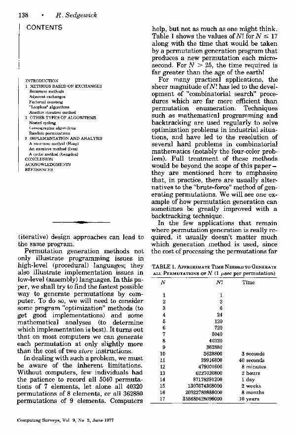
help, but not as much as one might think. Table 1 shows the values of N! for N -< 17 along with the time that would be taken by a permutation generation program that produces a new permutation each micro- second. For N > 25, the time required is far greater than the age of the earth!
For many practical applications, the sheer magnitude of N! has led to the devel- opment of "combinatorial search" proce- dures which are far more efficient than permutation enumeration. Techniques such as mathematical programming and backtracking are used regularly to solve optimization problems in industrial situa- tions, and have led to the resolution of several hard problems in combinatorial mathematics (notably the four-color prob- lem). Full t reatment of these methods would be beyond the scope of this p a p e r - they are mentioned here to emphasize that, in practice, there are usually alter- natives to the "brute-force" method of gen- erating permutations. We will see one ex- ample of how permutation generation can sometimes be greatly improved with a backtracking technique.
In the few applications that remain where permutation generation is really re- quired, it usually doesn't matter much which generation method is used, since the cost of processing the permutations far
T A B L E 1. APPROXIMATE TIME NEEDED TO GENERATE ALL PERMUTATIONS OF N (1 /zsec pe r p e r m u t a t i o n )
N NI T i m e
1 1 2 2 3 6 4 24 5 120 6 720 7 5040 8 40320 9 362880
10 3628800 11 39916800 12 479001600 13 6227020800 14 87178291200 15 1307674368000 16 20922789888000 17 355689428096000
3 seconds 40 seconds
8 m i n u t e s 2 h o u r s 1 day 2 weeks 8 m o n t h s
10 y e a r s
Computing Surveys, Vol 9, No 2, June 1977
P e r m u t a t i o n Genera t ion M e t h o d s • 139
exceeds the cost of generating them. For example, to evaluate the performance of an operating system, we might want to try all different permutations of a fLxed set of tasks for processing, but most of our time would be spent simulating the processing, not generating the permutations. The same is usually true in the study of combi- natorial properties of permutations, or in the analysis of sorting methods. In such applications, it can sometimes be worth- while to generate "random" permutations to get results for a typical case. We shall examine a few methods for doing so in this paper.
In short, the fastest possible permuta- tion method is of limited importance in practice. There is nearly always a better way to proceed, and if there is not, the problem becomes really hopeless when N is increased only a little.
Nevertheless, permutation generation provides a very instructive exercise in the implementation and analysis of algo- rithms. The problem has received a great deal of attention in the literature, and the techniques that we learn in the process of carefully comparing these interesting al- gorithms can later be applied to the per- haps more mundane problems that we face from day to day.
We shall begin with simple algorithms that generate permutations of an array by successively exchanging elements; these algorithms all have a common control structure described in Section 1. We then will study a few older algorithms, includ- ing some based on elementary operations other than exchanges, in the framework of this same control structure (Section 2). Fi- nally, we shall treat the issues involved in the implementation, analysis, and "opti- mization" of the best of the algorithms (Section 3).
1. METHODS BASED ON EXCHANGES
A natural way to permute an array of elements on a computer is to exchange two of its elements. The fastest permutation algorithms operate in this way: All N! per- mutations of N elements are produced by a sequence of N ! - 1 exchanges. We shall use the notation
P[1]:=:P[2]
to mean "exchange the contents of array elements P[1] and P[2]". This instruction gives both arrangements of the elements P[1], P[2] (i.e., the arrangement before the exchange and the one after). For N = 3, several different sequences of five ex- changes can be used to generate all six permutations, for example
P[1] =:P[2] P[2]:=:P[3] P[1] =:P[2] P[2]-=:P[3] P[1]:=-P[2].
If the initial contents of P[1] P[2] P[3] are A B C, then these five exchanges will pro- duce the permutations B A C, B C A, C B A , C A B, a n d A C B.
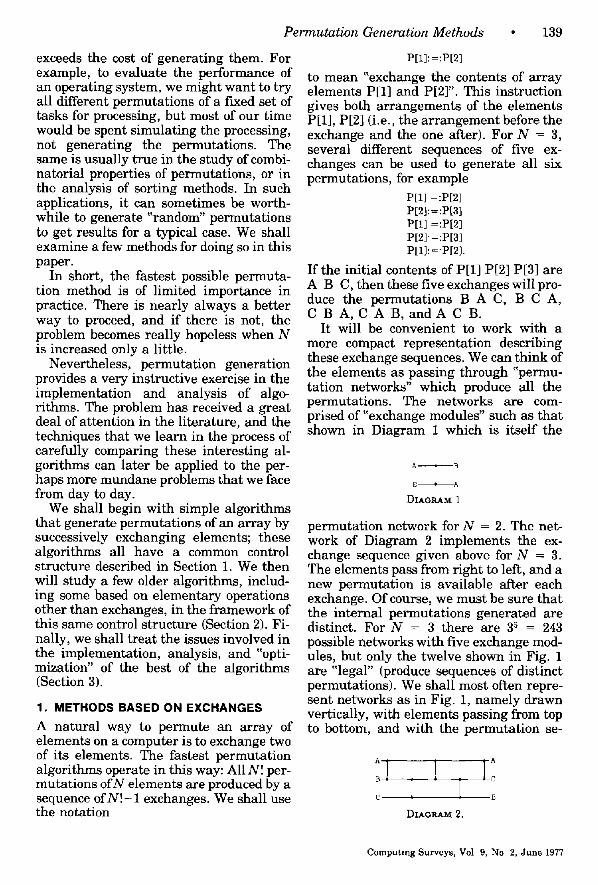
It will be convenient to work with a more compact representation describing these exchange sequences. We can think of the elements as passing through "permu- tation networks" which produce all the permutations. The networks are com- prised of "exchange modules" such as that shown in Diagram 1 which is itself the
DIAGRAM 1
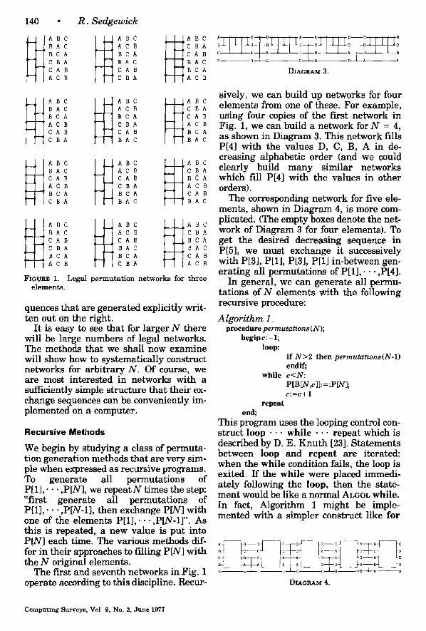
permutation network for N = 2. The net- work of Diagram 2 implements the ex- change sequence given above for N = 3. The elements pass from right to left, and a new permutation is available after each exchange. Of course, we must be sure that the internal permutations generated are distinct. For N = 3 there are 35 = 243 possible networks with five exchange mod- ules, but only the twelve shown in Fig. 1 are "legal" (produce sequences of distinct permutations). We shall most often repre- sent networks as in Fig. 1, namely drawn vertically, with elements passing from top to bottom, and with the permutation se-
:I I DIAGRAM 2.
Computing Surveys, Vol 9, No 2, June 1977
140 • R . Sedgewick
~ABC ~ABC ABC BAC ACB 'CBA BCA BCA --'CAB CBA BAC 'BAC CAB CAB 'BCA ACB CBA ACB
~ A B C ~ A BC ~A B C BAC ACB CBA BCA BCA CAB ACB CBA ACB CAB CAB BCA CBA BAC BAC
~ABC ~ABC ABC BAC ACB ~ CBA CAB CAB BCA ACB CBA ACB BCA BCA ~ CAB CBA BAC BAC
~ A B C ~ A B C ~A BC BAC ACB CBA CAB CAB BCA CBA BAC BAC BCA BCA CAB ACB CBA ACB
FIGURE 1. Legal permuta t ion networks for three elements.
quences that are generated explicitly writ- ten out on the right.
It is easy to see that for larger N there will be large numbers of legal networks. The methods that we shall now examine will show how to systematically construct networks for arbitrary N. Of course, we are most interested in networks with a sufficiently simple structure that their ex- change sequences can be conveniently im- plemented on a computer.
Recursive Methods
We begin by studying a class of permuta- tion generation methods that are very sim- ple when expressed as recursive programs. To generate all permutations of PIll, • • • ,PIN], we repeat N times the step: "first generate all permutations of P[1],- • • ,P[N-1], then exchange P[N] with one of the elements P[1],. . . ,P[N-1]". As this is repeated, a new value is put into P[N] each time. The various methods dif- fer in their approaches to f'filing P[N] with the N original elements.
The first and seventh networks in Fig. 1 operate according to this discipline. Recur-
A C D A--A D--D B
o ciEB o-VA ^ D ~ G ~ 3.
sively, we can build up networks for four elements from one of these. For example, using four copies of the f'Lrst network in Fig. 1, we can build a network for N = 4, as shown in Diagram 3. This network fills P[4] with the values D, C, B, A in de- creasing alphabetic order (and we could clearly build many similar networks which fill P[4] with the values in other orders).
The corresponding network for five ele- ments, shown in Diagram 4, is more com- plicated. (The empty boxes denote the net- work of Diagram 3 for four elements). To get the desired decreasing sequence in P[5], we must exchange it successively with P[3], P[1], P[3], P[1] in-between gen- erating all permutations of P[1] , . . . ,P[4].
In general, we can generate all permu- tations of N elements with the following recursive procedure:
Algori thm 1. procedure permutations (N);
begin c: = 1; loop:
if N > 2 then permutatmns(N-1) endif;
while c<N: P[B [N,c]]:=:P[N]; c:=c+l
repeat end;
This program uses the looping control con- struct loop • • • while • • • repeat which is described by D. E. Knuth [23]. Statements between loop and repeat are iterated: when the while condition fails, the loop is exited. If the while were placed immedi- ately following the loop, then the state- ment would be like a normal ALGOL while. In fact, Algorithm 1 might be imple- mented with a simpler construct like for
~ ~-c--c J ~E~EJ ~^ ^' c~
E E ~ D D ~ C C B ^
DIAO~M 4.
Computang Surveys, Vol 9, No. 2, June 1977
P e r m u t a t i o n Generat ion Me thods • 141
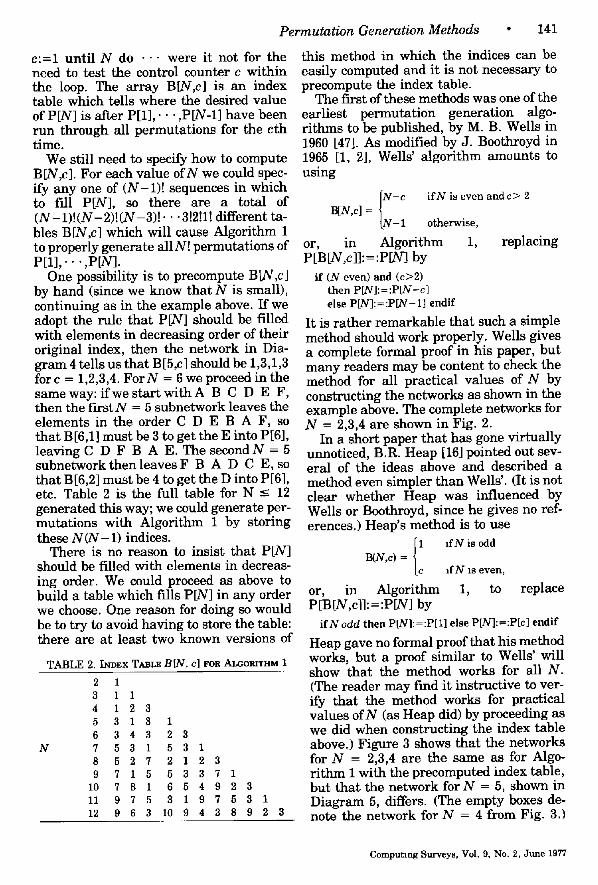
c:=1 until N do . ' - were it not for the need to test the control counter c within the loop. The array B[N,c] is an index table which tells where the desired value of P[N] is after P[1],. • • ,P[N-1] have been run through all permutations for the cth time.
We still need to specify how to compute B[N,c]. For each value of N we could spec- ify any one of (N- l ) ! sequences in which to fill P[N], so there are a total of ( N - 1 ) ! ( N - 2 ) ! ( N - 3 ) ! . • • 3!2!1! different ta- bles B[N,c] which will cause Algorithm 1 to properly generate allN! permutations of P[1], • . . ,P[N].
One possibility is to precompute BIN,c] by hand (since we know that N is small), continuing as in the example above. If we adopt the rule that P[N] should be filled with elements in decreasing order of their original index, then the network in Dia- gram 4 tells us that B[5,c] should be 1,3,1,3 for c = 1,2,3,4. ForN = 6 we proceed in the same way: if we start wi thA B C D E F, then the l~Lrst N = 5 subnetwork leaves the elements in the order C D E B A F, so that B[6,1] must be 3 to get the E into P[6], leaving C D F B A E. The second N = 5 subnetwork then leaves F B A D C E, so that B[6,2] must be 4 to get the D into P[6], etc. Table 2 is the full table for N <- 12 generated this way; we could generate per- mutations with Algorithm 1 by storing these N ( N - 1) indices.
There is no reason to insist that P[N] should be filled with elements in decreas- ing order. We could proceed as above to build a table which fills P[N] in any order we choose. One reason for doing so would be to try to avoid having to store the table: there are at least two known versions of
TABLE 2. I_~EX TA~LE B[N, c] FOa AJP,_,oRrrHM 1
N
2 1 3 1 1 4 1 2 3 5 3 1 3 1 6 3 4 3 2 3 7 5 3 1 5 3 8 5 2 7 2 1 9 7 1 5 5 3
1 0 7 8 1 6 5 1 1 9 7 5 3 1 1 2 9 6 3 1 0 9
1 2 3 3 7 1 4 9 2 3 9 7 5 3 4 3 8 9
1 2 3
this method in which the indices can be easily computed and it is not necessary to precompute the index table.
The fLrst of these methods was one of the earliest permutation generation algo- ri thms to be published, by M. B. Wells in 1960 [47]. As modified by J. Boothroyd in 1965 [1, 2], Wells' algorithm amounts to using
/ ~ - c i fN is even and c> 2 t~N,c]
- 1 otherwise,
or, in Algorithm 1, replacing P[B[N,c ]]:=:P[N] by
if (N even) and (c>2) then P[N]:=:P[N-c] else P[N]:=:P[N-1] endif
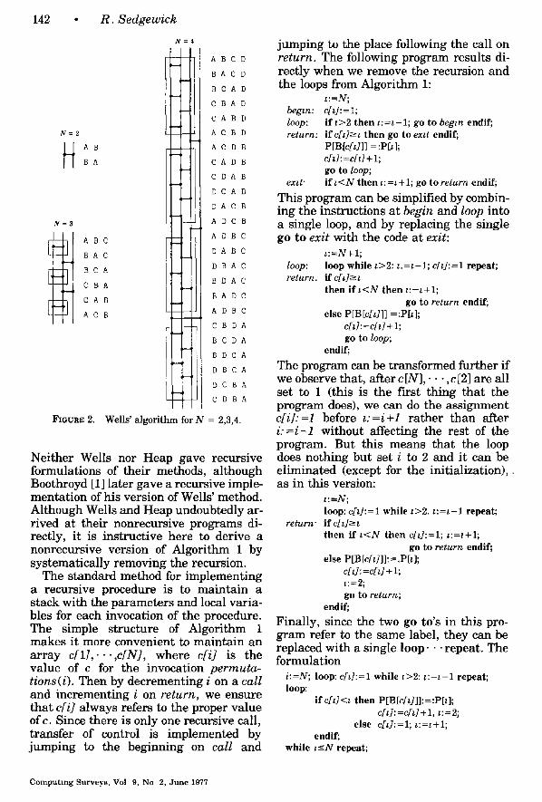
It is rather remarkable that such a simple method should work properly. Wells gives a complete formal proof in his paper, but many readers may be content to check the method for all practical values of N by constructing the networks as shown in the example above. The complete networks for N = 2,3,4 are shown in Fig. 2.
In a short paper that has gone virtually unnoticed, B.R. Heap [16] pointed out sev- eral of the ideas above and described a method even simpler than Wells'. (It is not clear whether Heap was influenced by Wells or Boothroyd, since he gives no ref- erences.) Heap's method is to use
B(N,c)=( I f iN is odd
l f Y is even,
or, in Algorithm 1, to replace P[B[N,c]]:=:P[N] by
i f N odd then P[N]:=:P[1] else P[N]:=:P[c] endif
Heap gave no formal proof that his method works, but a proof similar to Wells' will show that the method works for all N. (The reader may find it instructive to ver- ify that the method works for practical values of N (as Heap did) by proceeding as we did when constructing the index table above.) Figure 3 shows that the networks for N = 2,3,4 are the same as for Algo- r i thm 1 with the precomputed index table, but that the network for N = 5, shown in Diagram 5, differs. (The empty boxes de- note the network for N = 4 from Fig. 3.)
Computing Surveys, Vol. 9, No. 2, June 1977
142 R. Sedgewick
N=4
ABCD
BACD
BCAD
CBAD
CABD
ACBD
AB ACDB
BA CADB
C DA B
DCAB
DAC B
A DC B
ADBC A BC
DA BC BAC
DBAC BCA
BDAC CBA
CAB BADC
ACB ADBC
CBDA
BCDA
BDCA
-- DBCA
DCBA
CDBA
=2,3,4.
N=2
H
N=
4j
FIGURE 2. Wells' algorithm for N
Neither Wells nor Heap gave recursive formulations of their methods, although Boothroyd [1] later gave a recursive imple- mentation of his version of Wells' method. Although Wells and Heap undoubtedly ar- rived at their nonrecursive programs di- rectly, it is instructive here to derive a nonrecursive version of Algorithm 1 by systematically removing the recursion.
The standard method for implementing a recursive procedure is to maintain a stack with the parameters and local varia- bles for each invocation of the procedure. The simple structure of Algorithm 1 makes it more convenient to maintain an array c [1 ] , . . . , c [N] , where c[i] is the value of c for the invocation permuta- tions(i). Then by decrementing i on a call and incrementing i on return, we ensure that c[i] always refers to the proper value ofc. Since there is only one recursive call, transfer of control is implemented by jumping to the beginning on call and
jumping to the place following the call on return. The following program results di- rectly when we remove the recursion and the loops from Algorithm 1:
t:=N; begtn: c[d:=l; loop: if t>2 then t := t -1 ; go to begtn end[f; return: if c[t]>-t then go to extt end[f;
P[B[c#]]] =:P[t]; c[~]:=c[t] + l; go to loop;
extt" if t < N then t: =t + 1; go to return end[f;
This program can be simplified by combin- ing the instructions at begin and loop into a single loop, and by replacing the single go to exit with the code at exit:
t :=N+l ; loop: loop while t>2: t .= t -1 ; c[t]:=l repeat; return, i f c[t]>-z
then if t < N then t := t+ l ; go to return end[f;
else P[B[c[t]]] =:Pit]; c[~]:=c[t] + l; go to loop;
end[f;
The program can be transformed further if we observe that, after c [N],. • . , c [2] are all set to 1 (this is the first thing that the program does), we can do the assignment c[i]:=l before t:=i+l rather than after i :=i-1 without affecting the rest of the program. But this means that the loop does nothing but set i to 2 and it can be eliminated (except for the initialization),. as in this version:
t:=N; loop: c[t]:=l while z>2. t :=t-1 repeat;
return" [f c[t]>-t then if t < N then c[z]:=l; ~:=t+l;
go to return end[f; else P[B[c[t]]]: =.P[t ];
c[d: =c[t] + 1; t:=2; go to return;
end[f;
Finally, since the two go to's in this pro- gram refer to the same label, they can be replaced with a single loop. • • repeat. The formulation
i:=N; loop: c[~]:=1 while t > 2 : t : = z - 1 repeat; loop:
[f c[t]<l then P[B[c[zJ]]:=:P[z]; c[t]:=c[z]+ 1, t:=2;
else c[t]:=l; t:=t+l; end[f;
while t<-N repeat;
Computing Surveys, Vol 9, No 2, June 1977

Permutation Generation Methods • 143
N = 2
B A
N = 3
i I A B e
! BA C
A e B
BOA
F I G U R E 3 .
N = 4
il !l
ABC D
BAC D
C A B D
A C B D
B C A D
C BAD
DBA C
B DA C
A DB C
DA BC
BADC
A BDC
AC DB
CADB
DACB
A DC B
C DA B
DCAB
DCBA
C DBA
B D e A
D B CA
C BDA
BC DA
2 ,3 ,4 . Heap's algorithm for N =
is attractive because it is symmetric: each time through the loop, either c[i] is initial- ized and i incremented, or c[i] is incre- mented and i initialized. (Note: in a sense, we have removed too many go to's, since now the program makes a redundant test i -< N after setting i: =2 in the then clause. This can be avoided in assembly language, as shown in Section 3, or it could be han- dled with an "event variable" as described in [24].) We shall examine the structure of this program in detail later.
The programs above merely generate all permutations of P[1],. • • ,P[N]; in order to do anything useful, we need to process each permutation in some way. The proc- essing might involve anything from sim- ple counting to a complex simulation. Nor-
-B B- ~C
-C C - -D
~D a ^
DIAGRAM 5.
really, this is done by turning the permu- tation generation program into a proce- dure which returns a new permutation each time it is called. A main program is then written to call this procedure N! times, and process each permutation. (In this form, the permutation generater can be kept as a library subprogram.) A more efficient way to proceed is to recognize that the permutation generation procedure is really the "main program" and that each permutation should be processed as it is generated. To indicate this clearly in our programs, we shall assume a macro called process which is to be invoked each time a new permutation is ready. In the nonre- cursive version of Algorithm 1 above, if we put a call to process at the beginning and another call to process after the exchange statement, then process will be executed N! times, once for each permutation. From now on, we will explicitly include such calls to process in all of our programs.
The same transformations that we ap- plied to Algorithm 1 yield this nonrecur- sive version of Heap's method for generat- ing and processing all permutations of P[1], • • • ,P[N]:
Algorithm 2 (Heap)
~:=N; loop: c[~]:=l while ~>2:~:=~-1 repeat; process; l oop '
if c/t] <t then i f t odd then k:=l else k:=c[t] end[f;
P[t]:=:P[k]; c[l]:=c[t] + l; ~:=2; process,
else c[~]:=l; ~:=~+1 end[f;
while I ~ N repeat;
This can be a most efficient algorithm when implemented properly. In Section 3 we examine further improvements to this algorithm and its implementation.
Adjacent Exchanges
Perhaps the most prominent permutation enumeration algorithm was formulated in 1962 by S. M. Johnson [20] and H. F. Trot- ter [45], apparently independently. They discovered that it was possible to generate all N! permutations of N elements with N! -1 exchanges of adjacent elements.
Computing Surveys, Col 9, No 2, June 1977
1 4 4 • R . Sedgewick
A---~ B B B B
i.!-Ti i ! E E ' E E T A
DL~GRAM 6
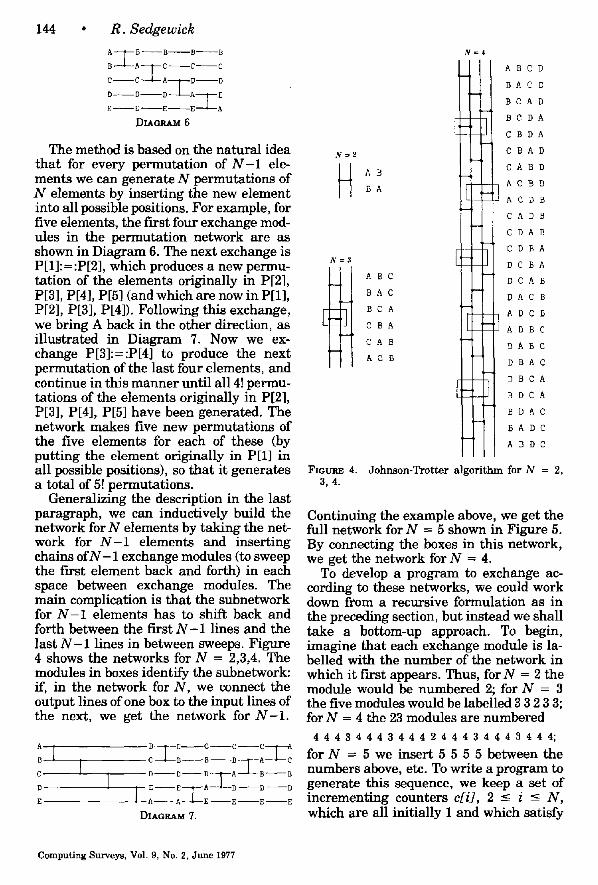
The method is based on the natural idea that for every permutation of N - 1 ele- ments we can generate N permutations of N elements by inserting the new element into all possible positions. For example, for five elements, the first four exchange mod- ules in the permutation network are as shown in Diagram 6. The next exchange is P[1]:=:P[2], which produces a new permu- tation of the elements originally in P[2], P[3], P[4], P[5] (and which are now in P[1], P[2], P[3], P[4]). Following this exchange, we bring A back in the other direction, as illustrated in Diagram 7. Now we ex- change P[3]:=:P[4] to produce the next permutation of the last four elements, and continue in this manner until all 4! permu- tations of the elements originally in P[2], P[3], P[4], P[5] have been generated. The network makes five new permutations of the five elements for each of these (by putting the element originally in P[1] in all possible positions), so that it generates a total of 5! permutations.
Generalizing the description in the last paragraph, we can inductively build the network for N elements by taking the net- work for N - 1 elements and inserting chains of N - 1 exchange modules (to sweep the first element back and forth) in each space between exchange modules. The main complication is that the subnetwork for N - 1 elements has to shift back and forth between the first N - 1 lines and the last N - 1 lines in between sweeps. Figure 4 shows the networks for N = 2,3,4. The modules in boxes identify the subnetwork: if, in the network for N, we connect the output lines of one box to the input lines of the next, we get the network for N - 1 .
A. I B
C-
D
E
: : 2 : T : T : : D I A a ~ 7.
Nffi4
N=2
H
N=
A B
B A
A BC
BA C
BCA
C BA
CAB
ACB
ABCD
BAC D
BCAD
BCDA
C BDA
C BA D
CABD
ACBD
A C DB
CADB
CDA B
CDBA
DC BA
DCAB
DAC B
ADCB
ADBC
D / k B C
D B A C
D B C A
B D C A
B D A C
BA DC
A B D C
FIGURE 4. Johnson-Tro t t e r a lgor i thm for N = 2, 3, 4.
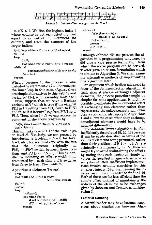
Continuing the example above, we get the full network for N = 5 shown in Figure 5. By connecting the boxes in this network, we get the network for N = 4.
To develop a program to exchange ac- cording to these networks, we could work down from a recursive formulation as in the preceding section, but instead we shall take a bottom-up approach. To begin, imagine that each exchange module is la- belled with the number of the network in which it first appears. Thus, for N = 2 the module would be numbered 2; for N = 3 the five modules would be labelled 3 3 2 3 3 ; for N = 4 the 23 modules are numbered
4 4 4 3 4 4 4 3 4 4 4 2 4 4 4 3 4 4 4 3 4 4 4 ; for N ~ 5 we insert 5 5 5 5 between the numbers above, etc. To write a program to generate this sequence, we keep a set of incrementing counters c[i], 2 < i <- N , which are all initially 1 and which satisfy
Computing Surveys, Vol. 9, No. 2, June 1977
P e r m u t a t i o n G e ne ra t i on M e t h o d s • 145
[ ~ ! I II llll II lllIl. II ]Ill ll.l i,,, :: ',,",',' ' " "
FIGURE 5 Johnson-Trot ter a lgori thm for N = 5.
1 < c[i] <- i. We fmd the highest index i whose counter is not exhausted (not yet equal to i), output it, increment its counter, and reset the counters of the larger indices:
i:=1; loop while i<-N: i:=~+1; c[i]:=l repeat; c[1]: =0; loop:
i :=N; loop while c[,]=i: c[i]:=l; i : = , - i repeat;
while ,>1: comment exchange module ~s on level ~ ;
c[~]:=c[~] + l repeat;
When i becomes 1, the process is com- p l e t ed - the statement c[1] = 0 terminates the inner loop in this case. (Again, there are simple alternatives to this with "event variables" [24], or in assembly language.)
Now, suppose that we have a Boolean variable d i N ] which is true if the original P[1] is travelling from P[1] down to P[N] and false if it is travelling from P[N] up to P[1]. Then, when i = N we can replace the comment in the above program by
if d[N] then k:=c[N] else k :=N-c[N] endif; P[k]:,= :P[k + 1];
This will take care of all of the exchanges on level N. Similarly, we can proceed by introducing a Boolean d [N-1] for level N - 1 , etc., but we must cope with the fact that the elements originally in P[2] , . . . ,PIN] switch between those loca- tions and P[1] , . . . ,P [N-1] . This is han- dled by including an offset x which is in- cremented by 1 each time a d[i] switches from false to true. This leads to:
A l g o r i t h m 3 (Johnson-Trotter) ~:=1; loop while ~<N: ~:=~+1; c[~]:=l;
d[i]:= true; repeat; c[1]:=0; process; loop:
i:=N; x:=0; loop while c[~]=~:
i f not d/~] then x:=x+l endif; d[i]:= not d/z]; c[d:=l; i .=~- l;
repeat;
while i>1: if d/~] then k:=c[~]+x
else k:=~-c[~]+x endif; P[k]:=:P[k + 1]; process; c[i]:=c[i] + l;
repeat;
Although Johnson did not present the al- gorithm in a programming language, he did give a very precise formulation from which the above program can be derived. Trotter gave an ALC~OL formulation which is similar to Algorithm 3. We shall exam- ine alternative methods of implementing this algorithm later.
An argument which is often advanced in favor of the Johnson-Trotter algorithm is that, since it always exchanges adjacent elements, the proc e s s procedure might be simpler for some applications. It might be possible to calculate the incremental effect of exchanging two elements ra ther than reprocessing the entire permutation. (This observation could also apply to Algorithms 1 and 2, but the cases when they exchange nonadjacent elements would have to be handled differently.)
The Johnson-Trotter algorithm is often inefficiently formulated [5, 10, 12] because it can be easily described in terms of the values of elements being permuted, rather than their positions. If P[1],. • ", P[N] are originally the integers 1 , - . . , N, then we might try to avoid maintaining the offset x by noting that each exchange simply in- volves the smallest integer whose count is not yet exhausted. Inefficient implementa- tions involve actually searching for this smallest integer [5] or maintaining the in- verse permutation in order to find it [10]. Both of these are far less efficient than the simple offset method of mgintaining the indices of the elements to be exchanged given by Johnson and Trotter, as in Algo- r i thm 3.
Factorial Counting A careful reader may have become suspi- cious about similarities between Algo-
Computing Surveys, Vol. 9, No. 2, June 1977
146 • R . Sedgewick
rithms 2 and 3. The similarities become striking when we consider an alternate implementation of the Johnson-Trotter method:
Algor i t hm 3a (Alternate Johnson-Trotter) z" =N; loop: c[t]:=l; d/l] :=true; while l > l : ~.=~ - 1 repeat; process, loop:
i f c[t] < N + l - I then if d / d then k.=c[~]+x
else k : = N + l - t - c [ t ] + x endif; P[k]: = :P [k + 1]; process; c[t]:=c[~]+l; ~:=1; x:=0; else if not d/t] then x :=x+l endif;
c[z]:=l; ~:=z+l; d[t]:= not d /d ; endif;
while ~-<N repeat;
This program is the result of two simple transformations on Algorithm 3. First, change i to N + I - ~ everywhere and rede- fme the c and d arrays so that c[N+l -~], d [N +1 - i ] in Algorithm 3 are the same as c[i], d[i] in Algorithm 3a. (Thus a refer- ence to c[i] in Algorithm 3 becomes c [ N + l - i ] when i is changed to N + I - i , which becomes c[i] in Algorithm 3a.) Sec- ond, rearrange the control structure around a single outer loop. The condition c[i] < N + l - i in Algorithm 3a is equiva- lent to the condition c[i] < i in Algorithm 3, and beth programs perform the ex- change and process the permutation in this case. When the counter is exhausted (c[i] = N + I - ~ in Algorithm 3a; c[i] = i in Algorithm 3), both programs fLx the offset, reset the counter, switch the direction, and move up a level.
If we ignore statements involving P, k and d, we fmd that this version of the Johnson-Trotter algorithm is identical to Heap's method, except that Algorithm 3a compares c[i] w i th N + I - i and Algorithm 2 compares it with i. (Notice that Algo- r i thm 2 still works properly ff in beth its occurrences 2 is replaced by I .)
To appreciate this similarity more fully, let us consider the problem of writing a program to generate all N-digit decimal numbers: to "count" from 0 to 9 9 . . . 9 = 10N-1. The algorithm that we learn in grade school is to increment the right-most
digit which is not 9 and change all the nines to its right to zeros. If the digits are stored in reverse order in the array c[N],c[N - 1], . . . ,c[2],c[1] (according to the way in which we customarily write numbers) we get the program
t :=N, loop c[~]:=O while t > l l : = ~ - I repeat; loop:
i f c[~]<9 then c[d:=c[t]+ l; z =1 else c[z]:=O; ~ = z + l
endif; while ~<-N repeat;
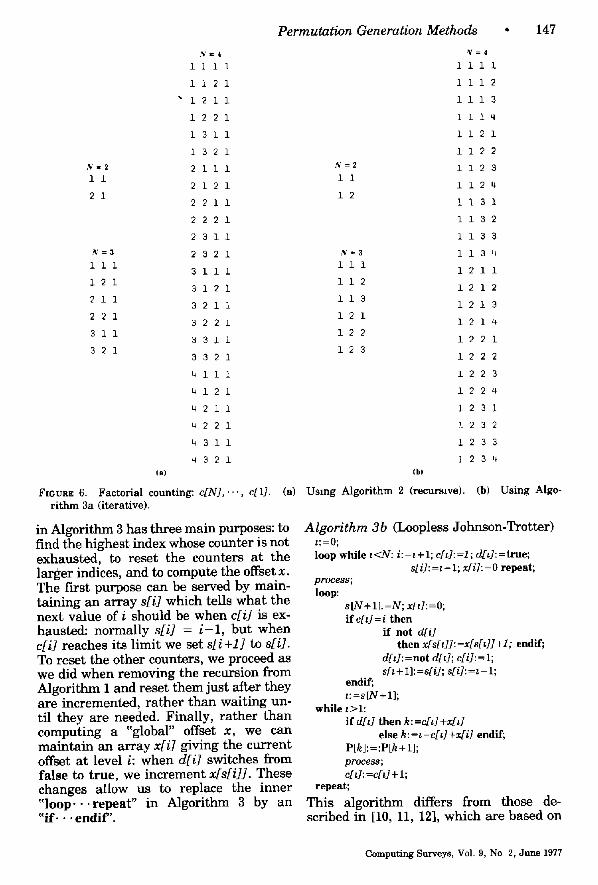
From this program, we see that our per- mutation generation algorithms are con- trolled by this simple counting process, but in a mixed-radix number system. Where in ordinary counting the digits satisfy 0 -< c[i] <- 9, in Algorithm 2 they satisfy 1 -< c[i] -< i and in Algorithm 3a they satisfy 1 <- c[i] <- N - i + l . Figure 6 shows the val- ues of c [ 1 ] , . . . ,c[N] when process is en- countered in Algorithms 2 and 3a for N = 2,3,4.
Virtually all of the permutation genera- tion algorithms that have been proposed are based on such "factorial counting" schemes. Although they appear in the lit- erature in a variety of disguises, they all have the same control structure as the elementary counting program above. We have called methods like Algorithm 2 re- cursive because they generate all se- quences of c[1] , . . . , c [ i -1] in-between in- crements of c[i] for all i; we shall call methods like Algorithm 3 iterative because they iterate c[i] through all its values in- between increments of c[i + 1], • • .,c[N].
Loopless Algorithms
An idea that has attracted a good deal of attention recently is that the Johnson- Trotter algorithm might be improved by removing the inner loop from Algorithm 3. This idea was introduced by G. Ehrlich [10, 11], and the implementation was re- fined by N. Dershowitz [5]. The method is also described in some detail by S. Even [12].
Ehrlich's original implementation was complex, but it is based on a few standard programming techniques. The inner loop
Computing Surveys, Vol 9, No 2, June 1977
N=4 i 111
1121
• 1211
1221
1311
1321
N - 2 2111 11
2121 21
2211
2221
2311
N = 3 2321
111 3111
121 3121
211 3211
221 3221
311 3311
321 3321
4111
4121
42 ll
4221
4811
4321 (a)
Fmu~ 6. Factorial counting: rithm 3a (iterative).
c[N], . . . , c[1]. (a)
P e r m u ~ n G e ~ r a ~ n M e t ~ • 147
~=4 iiii
1112
1113
1114
1121
1122
N = 2 1123 ii
1124 12
1131
1132
1133
N = 3 1134
iii 1211
112 1212
113 1213
121 1214
122 1221
123 1222
1223
1224
1231
1 2 3 2
1 2 3 3
1 2 3 4 (b)
Using Mgorithm 2 ( r e c ~ l v e ) . (b) Using M g o -
in Algorithm 3 has three main purposes: to find the highest index whose counter is not exhausted, to reset the counters at the larger indices, and to compute the offset x. The first purpose can be served by main- taining an array s[i] which tells what the next value of i should be when c[i] is ex- hausted: normally s[i] = i - 1 , but when c[i] reaches its limit we set s [ i + l ] to s[i]. To reset the other counters, we proceed as we did when removing the recursion from Algorithm 1 and reset them just a l~r they are incremented, rather than waiting un- til they are needed. Finally, rather than computing a "global" offset x, we can maintain an array x[i] giving the current offset at level i: when d[i] switches from false to true, we increment x[s[i]]. These changes allow us to replace the inner "loop. . .repeat" in Algorithm 3 by an "ft. • • endif'.
Algor i thm 3b (Loopless Johnson-Trotter) : :=0; loop while : < N : i: = : + 1; c[d: =1 ; d / d : =true;
s[i]:=:- l; x[i]:=O repeat; process; loop:
s[N + I].=N; x / : ] :=0 ; i f c[Q = i then
if not d/ i ] then x[s[ Q] : =x[s[ Q] +1; endif;
d/t]: =not d/d; c[i]: = 1; s i t + 1]: =s[i]; s[i]: = : - 1;
endff; t:=s[N + l ];
while :>1: if d /d then k: =c[~]+x[d
else k: =:-c[d+x[i] endif; P[k] := :P[k + 1]; process; c[Q: =c[d + 1;
repeat;
This algorithm differs from those de- scribed in [10, 11, 12], which are based on
Computing Surveys, Vol. 9, No 2, June 1977
148 * R. Sedgewick
the less efficient implementations of the Johnson-Trotter algorithm mentioned above. The loopless formulation is pur- ported to be an improvement because each iteration of the main loop is guaranteed to produce a new permutation in a ffLxed number of steps.
However, when organized in this form, the unfortunate fact becomes apparent that the loopless Algorithm 3b is slower than the normal Algorithm 3. Loopfree im- plementation is not an improvement at all! This can be shown with very little analysis because of the similar structure of the al- gorithms. If, for example, we were to count the total number of times the statement c[i]:=l is executed when each algorithm generates all N! permutations, we would find that the answer would be exactly the same for the two algorithms. The loopless algorithm does not eliminate any such as- signments; it just rearranges their order of execution. But this simple fact means that Algorithm 3b must be slower than Algo- r i thm 3, because it not only has to execute all of the same instructions the same num- ber of times, but it also suffers the over- head of maintaining the x and s arrays.
We have become accustomed to the idea that it is undesirable to have programs with loops that could iterate N times, but this is simply not the case with the John- son-Trotter method. In fact, the loop iter- ates N times only once out of the N! times that it is executed. Most often (N-1 out of every N times) it iterates only once. If N were very large it would be conceivable that the very few occasions that the loop iterates many times might be inconven- ient, but since we know that N is small, there seems to be no advantage whatso- ever to the loopless algorithm.
Ehrlich [10] found his algorithm to run "twice as fast" as competing algorithms, but this is apparently due entirely to a simple coding technique (described in Sec- tion 3) which he applied to his algorithm and not to the others.
Another Iterative Method
In 1976, F. M. Ives [19] published an ex- change-based method like the Johnson- Trotter method which does represent an improvement. For this method, we build
I I ~ - ^ :[: __l T il[l I : L_:
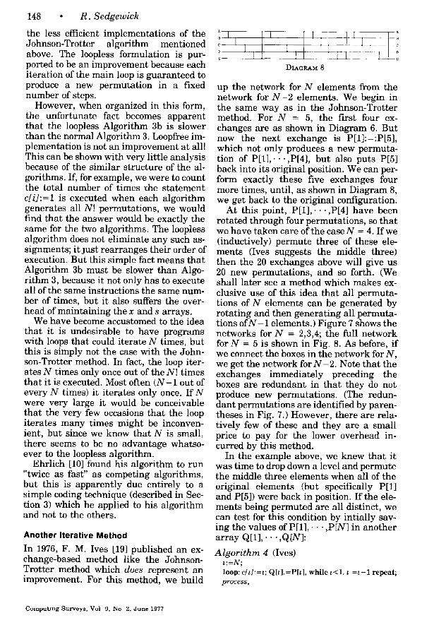
DIAGRAM 8
up the network for N elements from the network for N - 2 elements. We begin in the same way as in the Johnson-Trotter method. For N = 5, the first four ex- changes are as shown in Diagram 6. But now the next exchange is P[1]:=:P[5], which not only produces a new permuta- tion of P[1], . . . ,P[4], but also puts P[5] back into its original position. We can per- form exactly these five exchanges four more times, until, as shown in Diagram 8, we get back to the original configuration.
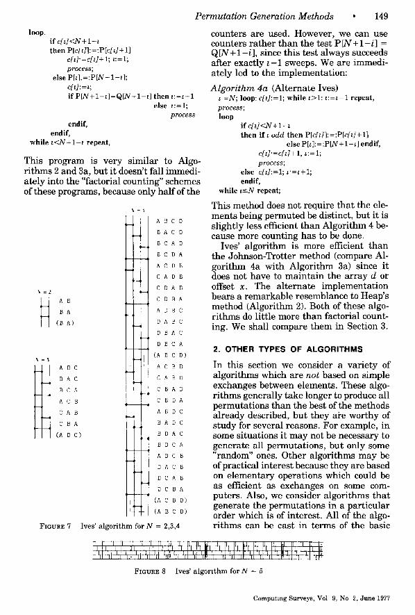
At this point, P[1] , . . . ,P[4] have been rotated through four permutations, so that we have taken care of the case N = 4. If we (inductively) permute three of these ele- ments (Ives suggests the middle three) then the 20 exchanges above will give us 20 new permutations, and so forth. (We shall later see a method which makes ex- clusive use of this idea that all permuta- tions of N elements can be generated by rotating and then generating all permuta- tions of N - 1 elements.) Figure 7 shows the networks for N = 2,3,4; the full network for N = 5 is shown in Fig. 8. As before, if we connect the boxes in the network for N, we get the network for N - 2 . Note that the exchanges immediately preceding the boxes are redundant in that they do not produce new permutations. (The redun- dant permutations are identified by paren- theses in Fig. 7.) However, there are rela- tively few of these and they are a small price to pay for the lower overhead in- curred by this method.
In the example above, we knew that it was time to drop down a level and permute the middle three elements when all of the original elements (but specifically P[1] and P[5]) were back in position. If the ele- ments being permuted are all distinct, we can test for this condition by intially sav- ing the values of P[1], • • • ,P[N] in another array Q[1],-. . ,Q[N]:
Algori thm 4 (Ives) ~:=N; loop: c[~]'=l; Q[~].=P[~], while ~<1. ~ =~-1 repeat; process,
Computing Surveys, Vol 9, No 2, June 1977
Permutation Generation Methods • 149
l oop . i f c[ t]<N + l - t t h e n P[c[t]]: =:P[c[t] + 1]
c[t]'=c[t]+ l; t : = l ;
process; e l s e P [ z ] . = : P [ N + 1 - t ] ;
c[t]: =t ;
i f P[N + I - t ]=Q[N + I - t ] t h e n t:=t + l e l se t : = l ;
process endi f ,
end i f , w h i l e t < N + l - z r e pe a t ,
This program is very similar to Algo- r i thms 2 and 3a, but it doesn't fall immedi- ately into the "factorial counting" schemes of these programs, because only hal f of the
% = 2
B A
(B A)
% = 4
.....-i
l
,• A BC A
B AC C
BC A
A C B C
CAB A
C BA
FmURE 7 Ires' a l g o r i t h m for N =
A BC D
BA C D
BC A D
BC DA
A C D B
C A D B
C DA B
C D B A
A D B C
DA BC
D B A C
D BC A
(A B C D)
C B D
A B D
C BAD
B DA
BDC
BA D C
B D A C
B D C A
A DC B
DA C B
DC A B
D C BA
(A C B D)
(A B C D)
2,3,4
counters are used. However, we can use counters rather than the test P [ N + I - i ] = Q [ N + 1 - i ] , since this test a lways succeeds after exactly t - 1 sweeps. We are immedi- ately led to the implementation:
Algorithm 4a (Alternate Ives) t =N; loop: c[z]:=l; w h i l e t > l : t : = t - 1 repea t , process; l o o p
i f c [ t ]<N + l - t t h e n i f t odd t h e n P[c[t]]:=:P[c[z]+l]
e l se P [ t ] : = : P [ N + l - t ] end i f , c[l]'=c[l]+ l, t : = l ;
process; e l s e c[z]:=l; t ' = t + l ;
endi f , w h i l e t -<N repeat ;
This method does not require that the ele- ments being permuted be distinct, but it is s l ight ly less efficient than Algori thm 4 be- cause more count ing has to be done.
Ives' a lgorithm is more efficient than the Johnson-Trotter method (compare Al- gori thm 4a wi th Algor i thm 3a) since it does not have to mainta in the array d or offset x. The alternate implementat ion bears a remarkable resemblance to Heap's method (Algorithm 2). Both of these algo- r i thms do little more than factorial count- ing. We shall compare them in Section 3.
2. OTHER TYPES OF ALGORITHMS
In this section we consider a variety of algorithms which are not based on simple exchanges between elements . These algo- r i thms general ly take longer to produce all permutat ions than the best of the methods already described, but they ave worthy of s tudy for several reasons. For example, in some s i tuations it may not be necessary to generate all permutations, but only some "random" ones. Other algorithms may be of practical interest because they are based on e lementary operations which could be as efficient as exchanges on some com- puters. Also, we consider algorithms that generate the permutat ions in a particular order which is of interest. All of the algo- r i thms can be cast in terms of the basic
r ii i[ ii 1,~1 ii ][ 1[ Ira 11 I[ II b I[ II II L,I II II II. Id. ]1 II 1I I~ i Jl ll, pl i~lt ~{iili]~ E::E ~l II Jl ~,l II JJ IJ ~l~ II [l ,~ ,[, ,I 1 ll, ll~ I~! l [ I I l ifl I J I l l ' i f [ I l } I ! 1 [ I )1 I I I l I q l l ' l g ~1 u [[ l[ [I t~ II 11 II I P I[ II i l ~1 ~ II II li I P II II II I P [I li ~ll Ig I I
FIGURE 8 Ives' a l g o r i t h m for N = 5
Computing Surveys, Vol 9, No 2, June 1977
150 • R . Sedgewick
"factorial counting" control structure de- scribed above.
Nested Cycling
As we saw when we examined Ives' algo- rithm, N different permutations of P[1],. • • ,P[N] can be obtained by rotating the array. In this section, we examine per- mutation generation methods which are based, solely on this operation. We assume that we have a primitive operation
rotate(i)
which does a cyclic left-rotation of the ele- ments P[1] , . . . ,P[ i ] . In other words, ro- tate(i) is equivalent to
t:=P[1]; k:=2; loop while k<t: P[k-1]:=P[k] repeat; P[i]: =t;
The network notation for rotate(5) is given by Diagram 9. This type of operation can be performed very efficiently on some com- puters. Of course, it will generally not be more efficient than an exchange, since ro- tate(2) is equivalent to P[1]:=:P[2].
B ~ - - C
c ~ D
E-'~
DIAGRAM 9.
The most straightforward way to make use of such an operation is a direct recur- sive implementation like Algorithm 1: procedure permutattons (N);
begin c:= 1; loop:
if N>2 then permutattons(N-1) end[f; rotate(N);
while c<N: process; C : = c + l
r e p e a t ;
end;
W h e n the r e c u r s i o n is r e m o v e d f rom t h i s p r o g r a m in the w a y t h a t r e m o v e d t he re- cursion from Algorithm 1, we get an old algori thm which was discovered by C. Tompkins and L. J. Paige in 1956 [44]:
A l g o r i t h m 5 (Tompkins-Paige) i.=N; loop: c[i]=l while t>2 : t := t -1 repeat; process;
loop: rotate(i) if c[t]<t then c[t]: =c[i]+ 1; i: =2;
process; else c[t]:=l; t :=t+l
end[f; while t<-N repeat;
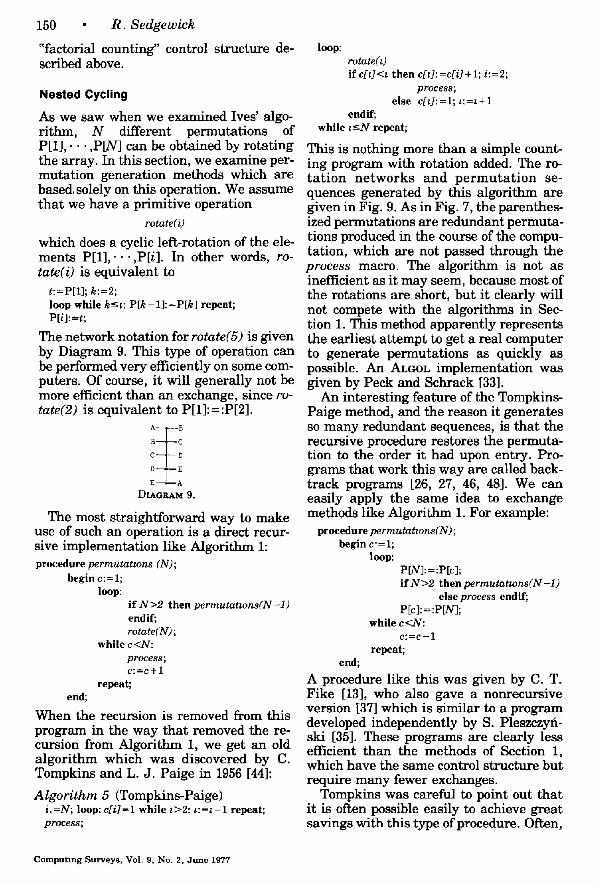
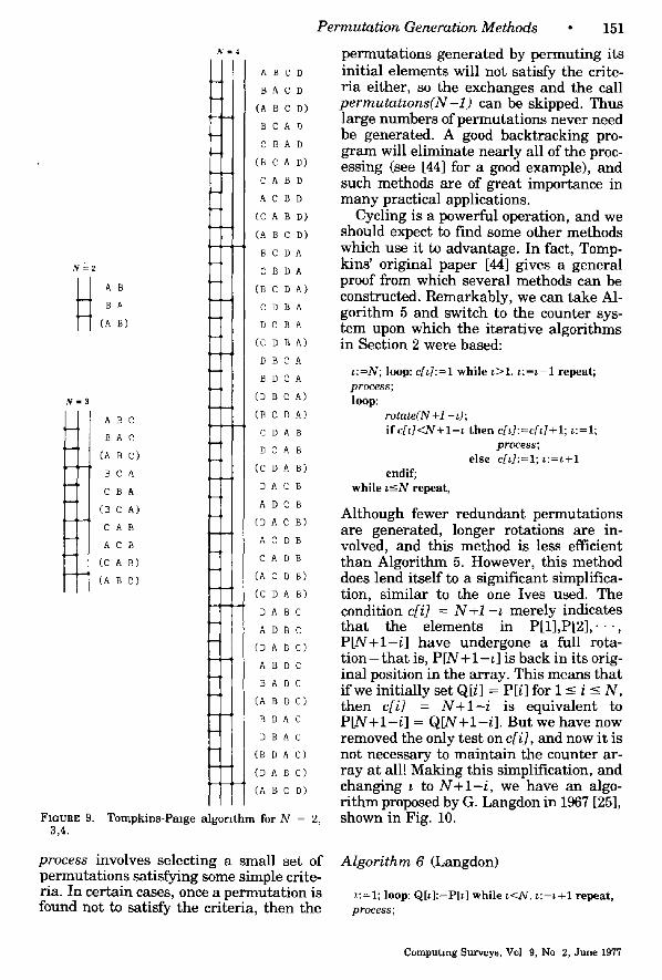
This is nothing more than a simple count- ing program with rotation added. The ro- t a t ion ne tworks and p e r m u t a t i o n se- quences generated by this algorithm are given in Fig. 9. As in Fig. 7, the parenthes- ized permutations are redundant permuta- tions produced in the course of the compu- tation, which are not passed through the process macro. The algorithm is not as inefficient as it may seem, because most of the rotations are short, but it clearly will not compete with the algorithms in Sec- tion 1. This method apparently represents the earliest at tempt to get a real computer to generate permutations as quickly as possible. An ALGOL implementation was given by Peck and Schrack [33].
An interesting feature of the Tompkins- Paige method, and the reason it generates so many redundant sequences, is that the recursive procedure restores the permuta- tion to the order it had upon entry. Pro- grams that work this way are called back- track programs [26, 27, 46, 48]. We can easily apply the same idea to exchange methods like Algorithm 1. For example:
procedure permutattons(N) ; begin c" = 1;
loop: P[N]:=:P[c]; if N>2 then permutatmns(N-1)
else process end[f; P[c ]: = :P[N];
while c<N: C : = C + I
repeat; end;
A procedure like this was given by C. T. Fike [13], who also gave a nonrecursive version [37] which is similar to a program developed independently by S. Pleszczyfi- ski [35]. These programs are clearly less efficient than the methods of Section 1, which have the same control structure but require many fewer exchanges.
Tompkins was careful to point out that it is often possible easily to achieve great savings with this type of procedure. Often,
Computing Surveys, Vol. 9, No. 2, June 1977
N=2
H N 3
--4
--4
¢
....,
FIGURE 9. 3,4.
A B
B A
(A B)
A BC
BA C
(A BC)
BCA
C BA
(B C A)
CAB
ACB
(C AB)
(A B C)
N=4
A B
BA
(A B
B C
C B
(B ¢
CA
AC
(C A
(A B
B C
C B
(B C
C D
DC
(C D
DB
B D
(D B
(B C
C D
DC
(C D
DA
A D
(DA
AC
CA
(A C
(C D
DA
A D
(D A
A B
B A
(A B
B D
D B
(B D
(D A
(A BC
Tompkins-Pa,ge algorithm for N
C D
C D
CD)
A O
A D
A D)
B D
B D
B D)
CD)
DA
DA
DA)
B A
BA
BA)
C A
CA
CA)
OA)
A B
h B
AB)
C B
C B
CB)
D B
DB
D B)
A B)
BC
BC
BC)
DC
D C
DC)
A C
A C
AC)
BC)
D)
= 2,
proces s involves selecting a small set of permutations satisfying some simple crite- ria. In certain cases, once a permutation is found not to satisfy the criteria, then the
P e r m u t a t i o n Genera t ion M e thods • 151
permutations generated by permuting its initial elements will not satisfy the crite- ria either, so the exchanges and the call p e r m u t a t m n s ( N - 1 ) can be skipped. Thus large numbers of permutations never need be generated. A good backtracking pro- gram will eliminate nearly all of the proc- essing (see [44] for a good example), and such methods are of great importance in many practical applications.
Cycling is a powerful operation, and we should expect to find some other methods which use it to advantage. In fact, Tomp- kins' original paper [44] gives a general proof from which several methods can be constructed. Remarkably, we can take Al- gorithm 5 and switch to the counter sys- tem upon which the iterative algorithms in Section 2 were based:
t:=N; loop: c[t]:=l w h i l e t > l . t : = t - 1 repeat; process; loop:
rotate(N +1 - t); i f c / d < N + l - t then c[t]:=c[t]+l; t : = l ;
process; else c[t]:=l; t : = t + l
endif; while z-<N repeat,
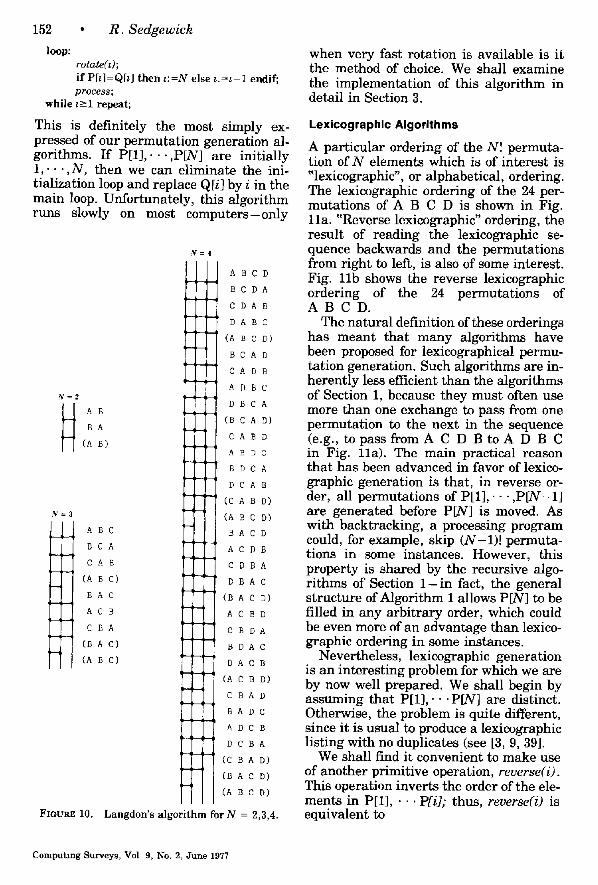
Although fewer redundant permutations are generated, longer rotations are in- volved, and this method is less efficient than Algorithm 5. However, this method does lend itself to a significant simplifica- tion, similar to the one Ives used. The condition c[i] = N + I - t merely indicates that the elements in P[1] ,P[2] , . . . , P [ N + I - i ] have undergone a full rota- t i o n - t h a t is, P[N+ l - t ] is back in its orig- inal position in the array. This means that if we initially set Q[i] = P[i] for 1 -< i <- N, then c[ i ] = N + l - i is equivalent to P [ N + I - i ] = Q [ N + I - i ] . But we have now removed the only test on c[ i ] , and now it is not necessary to maintain the counter ar- ray at all! Making this simplification, and changing t to N + I - i , we have an algo- rithm proposed by G. Langdon in 1967 [25], shown in Fig. 10.
A l g o r i t h m 6 (Langdon)
t : = l ; loop: Q[I ] :=P[~] while t < N . ~ : = t + l repeat, process;
Computing Surveys, Vol 9, No 2, June 1977
152 • R. Sedgewick
loop: rotate(t); i f P[z]=Q[t] then t : = N else t . = t - 1 endif; process;
while t->l repeat;
This is definitely the most simply ex- pressed of our permutation generation al- gorithms. If P [ 1 ] , . . . , P [ N ] are initially 1 , . . . , N , then we can eliminate the ini- tialization loop and replace Q[i] by i in the main loop. Unfortunately, this algorithm runs slowly on most computers -on ly
N=2
B A
(A B)
N =
FIGURE 10.
A BC
B C A
CAB
(A B C)
BAC
AC B
CBA
(B A C)
(A B C)
N=4
A
B
C
D
(A
B
C
A
D
(B
C
A
B
D
(C A
(A B
BA
A C
C D
D B
(B A
A C
C B
B D
DA
(A C
C B
BA
AD
D C
(C B
(BA
BC D
C DA
DAB
A B C
B C D)
C A D
A D B
DBC
B C A
CAD)
ABD
B D C
DCA
CAB
B D)
C D)
C D
D B
BA
A C
CD)
B D
DA
A C
C B
B D)
A D
D C
C B
BA
A D)
CD)
(A B C D)
Langdon's algorithm for N = 2 , 3 , 4 .
when very fast rotation is available is it the method of choice. We shall examine the implementation of this algorithm in detail in Section 3.
Lexicographic Algorithms
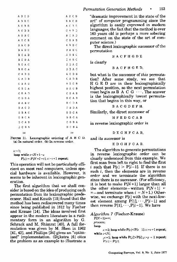
A particular ordering of the N! permuta- tion of N elements which is of interest is "lexicographic", or alphabetical, ordering. The lexicographic ordering of the 24 per- mutations of A B C D is shown in Fig. l la . "Reverse lexicographic" ordering, the result of reading the lexicographic se- quence backwards and the permutations from right to left, is also of some interest. Fig. l lb shows the reverse lexicographic ordering of the 24 permutations of A B C D .
The natural definition of these orderings has meant that many algorithms have been proposed for lexicographical permu- tation generation. Such algorithms are in- herently less efficient than the algorithms of Section 1, because they must often use more than one exchange to pass from one permutation to the next in the sequence (e.g., to pass from A C D B to A D B C in Fig. l la). The main practical reason that has been advanced in favor of lexico- graphic generation is that, in reverse or- der, all permutations of P [ 1 ] , . - - , P I N - l ] are generated before P[N] is moved. As with backtracking, a processing program could, for example, skip ( N - l ) ! permuta- tions in some instances. However, this property is shared by the recursive algo- rithms of Section 1 - in fact, the general structure of Algorithm 1 allows P[N] to be filled in any arbitrary order, which could be even more of an advantage than lexico- graphic ordering in some instances.
Nevertheless, lexicographic generation is an interesting problem for which we are by now well prepared. We shall begin by assuming that P [ 1 ] , . . . P [ N ] are distinct. Otherwise, the problem is quite different, since it is usual to produce a lexicographic listing with no duplicates (see [3, 9, 39].
We shall fmd it convenient to make use of another primitive operation, reverse(i). This operation inverts the order of the ele- ments in P[1], • • • P[i]; thus, reverse(i) is equivalent to
Computing Surveys, Vol 9, No. 2, June 1977
ABCD ABCD
ABDC BACD
ACBD ACBD
ACDB CABD
ADBC BCAD
ADCB CBAD
BACD ABDC
BADC BADC
BCAD ADBC
BCDA DABC
BDAC BDAC
BDCA DBAC
CABD ACDB
CADB CADB
CBAD ADCB
CBDA DACB
CDAB CDAB
CDBA DCAB
DABC BCDA
DACB CBDA
DBAC BDCA
DBCA DBCA
DCAB CDBA
DCBA DCBA
(a) (b)
~o t ra~ 11. ~ m ~ g r a p ~ c o ~ e H n g of A B C D. (a) In na tura l o ~ e r . (b) In r e v e r ~ order.
~:=i;
loop w h i l e ~<N+I -~ : P[~]:=:P[N+I-~]; ~:=t+l repeat;
This operation will not be particularly effi- cient on most real computers, unless spe- cial hardware is available. However, it seems to be inherent in lexicographic gen- eration.
The furst algorithm that we shall con- sider is based on the idea of producing each permutation from its lexicographic prede- cessor. Hall and Knuth [15] found that the method has been rediscovered many times since being published in 1812 by Fischer and Krause [14]. The ideas involved first appear in the modern l i terature in a rudi- mentary form in an algorithm by G. Schrack and M. Shimrat [40]. A full for- mulation was given by M. Shen in 1962 [41, 42], and Phillips [34] gives an "optim- ized" implementation. (Dijkstra [6] cites the problem as an example to illustrate a
Permutat ion Generation Methods • 153
"dramatic improvement in the state of the art" of computer programming since the algorithm is easily expressed in modern languages; the fact tha t the method is over 160 years old is perhaps a more sobering comment on the state of the ar t of com- puter science.)
The direct lexicographic successor of the permutation
B A C F H G D E
is clearly B A C F H G E D ,
but what is the successor of this permuta- tion? After some study, we see that H G E D are in their lexicographically highest position, so the next permutat ion must begin as B A C G • • -. The answer is the lexicographically lowest permuta- tion that begins in this way, or
B A C G D E F H .
Similarly, the direct successor of
H F E D G C A B
in reverse lexicographic order is
D E G H F C A B ,
and its successor is
E D G H F C A B .
The algorithm to generate permutations in reverse lexicographic order can be clearly understood from this example. We first scan from lei~ to right to fred the first i such that P[~] > P[ i -1] . If there is no such i, then the elements are in reverse order and we terminate the algorithm since there is no successor. (For efficiency, it is best to make P[N+I] larger than all the other e l e m e n t s - w r i t t e n P[N+I] = ~ - a n d terminate when i = N + I . ) Other- wise, we exchange P[i] with the next-low- est element among P [ 1 ] , . . - , P [ i - 1 ] and then reverse P[1],. • • ,P[i-1] . We have
Algor i thm 7 (Fischer-Krause) P [ N + I ] = ~ ; process; loop.
t:=2; loop while P[~]<P[~-I]: ~:=~+1 repeat; while t<N;
j : = l ; loop while P[ j ]>P[ i ] : j := j + 1 repeat; P[~]:=:P~];
Computing Surveys, Vol. 9, No 2, June 1977
154 • R . S e d g e w i c k
reverse(~ -1); process;
repeat;
Like the Tompkins-Paige algorithm, this algorithm is not as inefficient as it seems, since it is most often scanning and revers- ing short strings.
This seems to be the first example we have seen of an algorithm which does not rely on ~'factorial counting" for its control structure. However, the control structure here is overly complex; indeed, factorial counters are precisely what is needed to eliminate the inner loops in Algorithm 7.
A more efficient algorithm can be de- rived, as we have done several times be- fore, from a recursive formulation. A sim- ple recursive procedure to generate the permutations of P[1] , . - . ,P[N] in reverse lexicographic order can be quickly devised:
procedure lexperms(N) ; begin c:= 1;
loop: if N > 2
then lexperms(N-1) end[f; while c<N:
P[N]:=:P[c]; reverse(N-i ) ; c:=c+ l;
repeat; end;
Removing the recursion precisely as we did for Algorithm 1, we get
A l g o r i t h m 8 (Ord-Smith) ~:=N; loop c[~].=l; while ~>2:~:=~-1 repeat; process; loop:
if c[l] <~ then P[~ ]:='P[c[l]], reverse(~-l ) , c[~]:=c[z]+ l; ~:=2; process;
else c[l]:=l; ~:=~+1 end[f;
while ~-<N repeat;
This algorithm was first presented by R. J. Ord-Smith in 1967 [32]. We would not ex- pect a priori to have a lexicographic algo- r i thm so similar to the normal algorithms, but the recursive formulation makes it ob- vious.
Ord-Smith also developed [31] a "pseudo-lexicographic" algorithm which consists of replacing P[~]:=:P[c[i]]; re- v e r s e ( i - i ) ; by reverse( i ) in Algorithm 8.
There seem to be no advantages to this method over methods like Algorithm 1. Howell [17, 18] gives a lexicographic method based on treat ing P[1], • • • ,P[N] as a base-N number, counting in base N, and rejecting numbers whose digits are not dis- tinct. This method is clearly very slow.
Random Permutations
I f N is so large that we could never hope to generate all permutations of N elements, it is of interest to study methods for gener- ating ~random" permutations of N ele- ments. This is normally done by establish- ing some one-to-one correspondence be- tween a permutat ion and a random num- ber between 0 a n d N ! - l . (A full t rea tment of pseudorandom number generation by computer may be found in [22].)
First, we notice tha t each number be- tween 0 and N ! - 1 can be represented in a mixed radix system to correspond to an array c [ N ] , c [ N - 1 ] , . • • ,c[2] with 0 -< c[i] <- ~-1 for 2 -< i -< N. For example, 1000 corresponds to 1 2 1 2 2 0 since 1000 = 6! + 2.5! + 4! + 2.3! + 2.2!. For 0 -< n < N!, we have n = c[2].1! + c[3].2! + . . . + c[N]. (N- l ) ! . This correspondence is easily established through standard radix con- version algorithms [22, 27, 47]. Alterna- tively, we could fill the array by putt ing a ~'random" number between 0 and i - 1 in c[i] for 2 <_ i <_ N .
Such arrays c [ N ] , c [ N - 1 ] , . . . , c [ 2 ] can clearly be generated by the factorial count- ing procedure discussed in Section 1, so that there is an implicit correspondence between such arrays and permutations of 1 2 . . . N. The algorithms that we shall examine now are based on more explicit correspondences.
The fLrst correspondence has been at- tr ibuted to M. Hall, Jr . , in 1956 [15], al- though it may be even older. In this corre- spendence, c[i] is defined to be the number of elements to the left of i which are smaller than it. Given an array, the fol- lowing example shows how to construct the corresponding permutation. To fmd the permutation of 1 2 • • • 7 correspond- ing to
1 2 1 2 2 0
Computing Surveys, Vol 9, No 2, June 1977
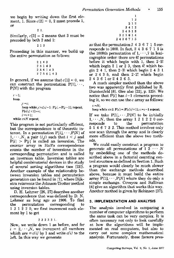
Permutation Generation Methods
we begin by writing down the first ele- ment, 1. Since c [2] = 0, 2 must precede 1, o r
2 1 .
Similarly, c [3] = 2 means that 3 must be preceded by both 2 and 1:
2 1 3
Proceeding in this manner, we build up the entire permutation as follows:
2 1 4 3 2 5 1 4 3 2 5 6 1 4 3 2 7 5 6 1 4 3
In general, if we assume that c[1] = 0, we can construct the permutation P[1] , . . . , P[N] with the program
v = l ; loop.
J:=~; loop whilej>c[~]+l: PO].=P[ j -1] ; repeat; P[c/l]+ 1]:=~; i ' =z+ l ;
while ~-<N repeat;
This program is not particularly efficient, but the correspondence is of theoretic in- terest. In a permutation P[1], . . - ,PIN] of 1,. • • ,N, a pair (i j ) such that i < j and P[i] > P0] is called an inversion. The counter array in Hall's correspondence counts the number of inversions in the corresponding permutation and is called an inversion table. Inversion tables are helpful combinatorial devices in the study of several sorting algorithms (see [23]). Another example of the relationship be- tween inversion tables and permutation generation can be found in [7], where Dijk- stra reinvents the Johnson-Trotter method using inversion tables.
D. H. Lehmer [26, 27] describes another correspondence that was def'med by D. N. Lehmer as long ago as 1906. To find the permutation corresponding to 1 2 1 2 2 0, we first increment each ele- ment by 1 to get
2 3 2 3 3 1 .
Now, we write down 1 as before, and for i = 2 , . - . , N , we increment all numbers which are -> c[i] by 1 and write c[i] to the left. In this way we generate
• 1 5 5
1 12
3 1 2 3 4 1 2
2 4 5 1 3 3 2 5 6 1 4
2 4 3 6 7 1 5
so that the permutation 2 4 3 6 7 1 5 cor- responds to 1000. In fact, 2 4 3 6 7 1 5 is the 1000th permutation of 1,. • • ,7 in lexi- cographic order: there are 6! permutations before it which begin with 1, then 2.5! which begin 2 1 or 2 3, then 4! which be- gin 2 4 1, then 2.3! which begin 2 4 3 1 or 2 4 3 5, and then 2.2! which begin 2 4 3 6 l o r 2 4 3 65 .
A much simpler method than the above two was apparently first published by R. Durstenfeld [8]. (See also [22], p. 125). We notice that P[i] has i - 1 elements preced- ing it, so we can use the c array as follows:
~:=N; loop while ~->2: P[~]:=:P[c[l]+l]; ~:=z-1 repeat;
If we take P[1], .-- ,P[N] to be initially 1 , . . . , N , then the array 1 2 1 2 2 0 cor- responds to the permutation 5 1 4 6 7 3 2. This method involves only one scan through the array and is clearly more efficient than the above two meth- ods.
We could easily construct a program to generate all permutations of 1 2 . . . N by embedding one of the methods de- scribed above in a factorial counting con- trol structure as defined in Section 1. Such a program would clearly be much slower than the exchange methods described above, because it must build the entire array P[1], .- . ,P[N] where they do only a simple exchange. Coveyou and Sullivan [4] give an algorithm that works this way. Another method is given by Robinson [37].
3. IMPLEMENTATION AND ANALYSIS
The analysis involved in comparing a number of computer algorithms to perform the same task can be very complex. It is often necessary not only to look carefully at how the algorithms will be imple- mented on real computers, but also to carry out some complex mathematical analysis. Fortunately, these factors pres-
Computing Surveys, Vol 9, No 2, June 1977
156 • R . S e d g e w i c k
ent less difficulty than usual in the case of permutation generation. First, since all of the algorithms have the same control structure, comparisons between many of them are immediate, and we need only examine a few in detail. Second, the anal- ysis involved in determining the total run- ning time of the algorithms on real com- puters (by counting the total number of times each instruction is executed) is not difficult, because of the simple counting algorithms upon which the programs are based.
If we imagine that we have an impor- tant application where all N! permuta- tions must be generated as fast as possible, it is easy to see that the programs must be carefully implemented. For example, if we are generating, say, every permutation of 12 elements, then every extraneous in- struction in the inner loop of the program will make it run at least 8 minutes longer on most computers (see Table 1).
Evidently, from the discussion in Sec- tion 1, Heap's method (Algorithm 2) is the fastest of the recursive exchange algo- rithms examined, and Ives' method (Algo- rithm 4) is the fastest of the iterative ex- change algorithms. All of the algorithms in Section 2 are clearly slower than these two, except possibly for Langdon's method (Algorithm 6) which may be competitive on machines offering a fast rotation capa- bility. In order to draw conclusions com- paring these three algorithms, we shall consider in detail how they can be imple- mented in assembly language on real com- puters, and we shall analyze exactly how long they can be expected to run.
As we have done with the high-level language, we shall use a mythical assem- bly language from which programs on real computers can be easily implemented. (Readers unfamiliar with assembly lan- guage should consult [21].) We shall use load (LD), stere (ST), add (ADD), subtract (SUB), and compare (CMP) instructions which have the general form
LABEL OPCODE REGISTER, OPERAND (optional)
The first operand will always be a sym- bolic register name, and the second oper- and may be a value, a symbolic register
name, or an indexed memory reference. For example, ADD 1,1 means "increment Register I by r'; ADD l,J means "add the contents of Register J to Register r'; and ADD I,C(J) means "add to Register I the contents of the memory location whose ad- dress is found by adding the contents of Register J to C". In addition, we shall use control transfer instructions of the form
OPCODE LABEL
namely JMP (unconditional transfer); JL, JLE, JE, JGE, JG (conditional transfer ac- cording as whether the first operand in the last CMP instruction was <, -<, =, ->, > than the second); and CALL (subroutine call). Other conditional jump instructions are of the form
OPCODE REGISTER, LABEL
namely JN, JZ, JP (transfer if the specified register is negative, zero, positive). Most machines have capabilities similar to these, and readers should have no diffi- culty translating the programs given here to particular assembly languages.
Much of our effort will be directed to- wards what is commonly called code opti- mization: developing assembly language implementations which are as efficient as possible. This is, of course, a misnomer: while we can usually improve programs, we can rarely "optimize" them. A disad- vantage of optimization is that it tends to greatly complicate a program. Although significant savings may be involved, it is dangerous to apply optimization tech- niques at too early a stage in the develop- ment of a program. In particular, we shall not consider optimizing until we have a good assembly language implementation which we have fully analyzed, so that we can tell where the improvements will do the most good. Knuth [24] presents a fuller discussion of these issues.
Many misleading conclusions have been drawn and reported in the literature based on empirical performance statistics com- paring particular implementations of par- ticular algorithms. Empirical testing can be valuable in some situations, but, as we have seen, the structures of permutation generation algorithms are so similar that the empirical tests which have been per-
Computing Surveys, Vol. 9, No 2, June 1977
Permutat ion Generation Methods • 157
formed have really been comparisons of compilers, programmers, and computers, not of algorithms. We shall see that the differences between the best algorithms are very subtle, and they will become most apparent as we analyze the assembly lan- guage programs. Fortunately, the assem- bly language implementations aren't much longer than the high-level descrip- tions. (This turns out to be the case with many algorithms.)
A Recursive Method (Heap)
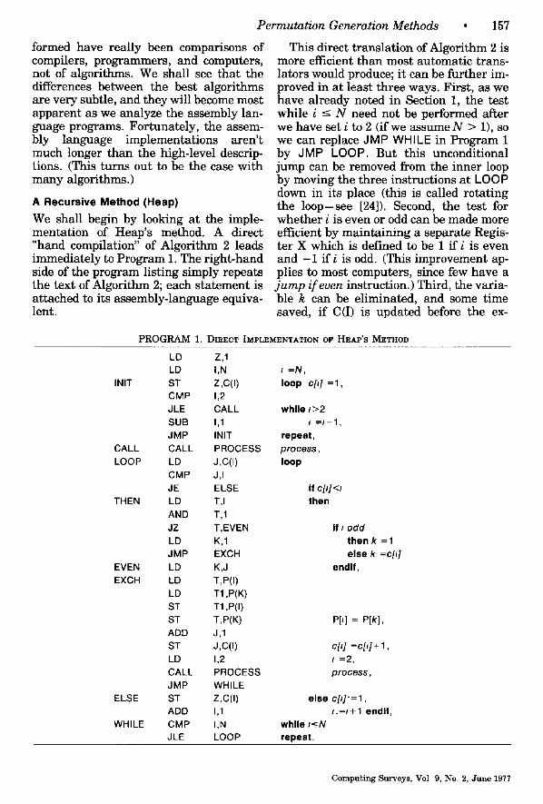
We shall begin by looking at the imple- mentation of Heap's method. A direct "hand compilation" of Algorithm 2 leads immediately to Program 1. The right-hand side of the program listing simply repeats the text of Algorithm 2; each statement is attached to its assembly-language equiva- lent.
This direct translation of Algorithm 2 is more efficient than most automatic trans- lators would produce; it can be further im- proved in at least three ways. First, as we have already noted in Section 1, the test w h i l e i -< N need not be performed after we have set i to 2 (if we assume N > 1), so we can replace JMP WHILE in Program 1 by JMP LOOP. But this unconditional jump can be removed from the inner loop by moving the three instructions at LOOP down in its place (this is called rotating the l oop - see [24]). Second, the test for whether i is even or odd can be made more efficient by maintaining a separate Regis- ter X which is defined to be 1 ff i is even and - 1 ff i is odd. (This improvement ap- plies to most computers, since few have a
j u m p i f even instruction.) Third, the varia- ble k can be eliminated, and some time saved, if C(I) is updated before the ex-
PROGRAM 1. DIRECT IMPLEMENTATION OF HEAP'S METHOD
LD Z,1 LD I,N
INIT ST Z,C(I) CMP 1,2 JLE CALL SUB 1,1 JMP INIT
CALL CALL PROCESS LOOP LD J,C(I)
CMP J,I JE ELSE
THEN LD T,I AND T,1 JZ T,EVEN LD K,1 JMP EXCH
EVEN LD K,J EXCH LD T,P(I)
LD T1 ,P(K) ST T1 ,P(I) ST T,P(K) ADD J,1 ST J,C(I) LD 1,2 CALL PROCESS JMP WHILE
ELSE ST Z,C(I) ADD 1,1
WHILE CMP I,N JLE LOOP
I = N ,
loop c[1] =1,
whi le />2 I =1-1 ,
repeat, process, loop
If c[/] then
if / odd then k =1 else k =c[i]
endlf,
P[I] = P[k],
ch] =cH+l, 1=2, process,
else c[11"= I , I . = i + I endlf,
whlle I-<N repeat,
Computing Surveys, Vol 9, No. 2, June 1977
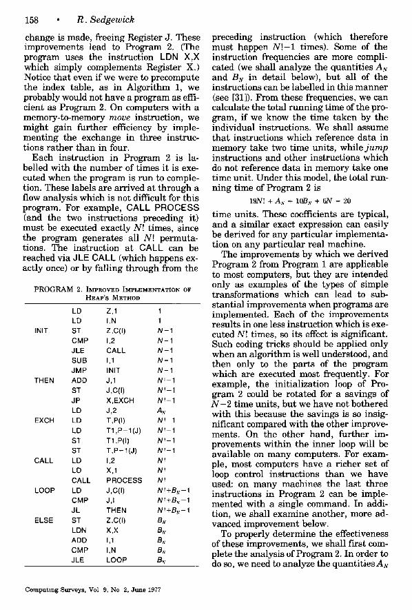
158 • R. Sedgewick
change is made, freeing Register J. These improvements lead to Program 2. (The program uses the instruction LDN X,× which simply complements Register X.) Notice that even if we were to precompute the index table, as in Algorithm 1, we probably would not have a program as effi- cient as Program 2. On computers with a memory-to-memory move instruction, we might gain further efficiency by imple- menting the exchange in three instruc- tions rather than in four.
Each instruction in Program 2 is la- belled with the number of times it is exe- cuted when the program is run to comple- tion. These labels are arrived at through a flow analysis which is not difficult for this program. For example, CALL PROCESS (and the two instructions preceding it) must be executed exactly N! times, since the program generates all N! permuta- tions. The instruction at CALL can be reached via JLE CALL (which happens ex- actly once) or by falling through from the
P R O G R A M 2. IMPROVED IMPLEMENTATION OF HEAP'S METHOD
LD Z,1 1 LD I,N 1
INIT ST Z,C(I) N - 1 CMP 1,2 N - 1 JLE CALL N - 1 SUB 1,1 N - 1 JMP INIT N - 1
THEN ADD J,1 N l - 1 ST J,C(I) NW-1 JP X,EXCH Nw-1 LD J,2 A N
EXCH LD T,P(I) Nw-1 LD T1 ,P - I ( J ) NV-1 ST T1,P(I) N w- 1 ST T , P - I ( J ) NW-1
CALL LD 1,2 NI LD X,1 NW CALL PROCESS Nw
LOOP LD J,C(I) NI+B~-I CMP J,I NI+BN-1 JL THEN NI+B~-I
ELSE ST Z,C(I) BN LDN X,X B~ ADD 1,1 B N CMP I,N BN JLE LOOP BN
preceding instruction (which therefore must happen N ! - I times). Some of the instruction frequencies are more compli- cated (we shall analyze the quantities AN and BN in detail below), but all of the instructions can be labelled in this manner (see [31]). From these frequencies, we can calculate the total running time of the pro- gram, if we know the time taken by the individual instructions. We shall assume that instructions which reference data in memory take two time units, while j u m p instructions and other instructions which do not reference data in memory take one time unit. Under this model, the total run- ning time of Program 2 is
19N! + A~ + 10BN + 6N - 20
time units. These coefficients are typical, and a similar exact expression can easily be derived for any particular implementa- tion on any particular real machine.
The improvements by which we derived Program 2 from Program 1 are applicable to most computers, but they are intended only as examples of the types of simple transformations which can lead to sub- stantial improvements when programs are implemented. Each of the improvements results in one less instruction which is exe- cuted N! times, so its effect is significant. Such coding tricks should be applied only when an algorithm is well understood, and then only to the parts of the program which are executed most frequently. For example, the initialization loop of Pro- gram 2 could be rotated for a savings of N - 2 time units, but we have not bothered with this because the savings is so insig- nificant compared with the other improve- ments. On the other hand, further im- provements within the inner loop will be available on many computers. For exam- ple, most computers have a richer set of loop control instructions than we have used: on many machines the last three instructions in Program 2 can be imple- mented with a single command. In addi- tion, we shall examine another, more ad- vanced improvement below.
To properly determine the effectiveness of these improvements, we shall first com- plete the analysis of Program 2. In order to do so, we need to analyze the quantities AN
Computing Surveys, Vol 9, No 2, June 1977
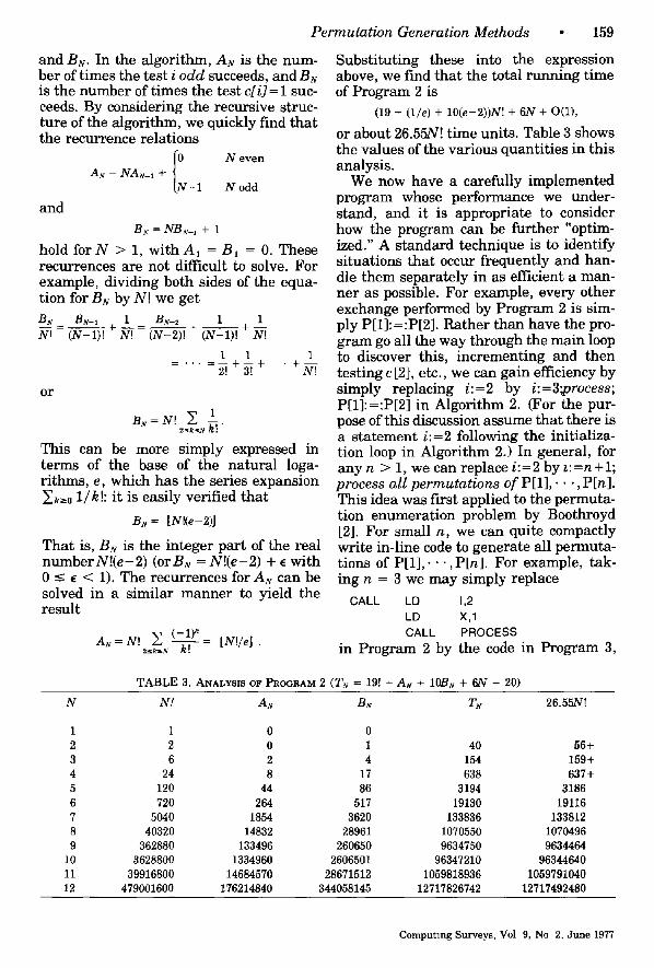
Permutation Generation Methods • 159
a n d B N. In the algorithm, A N is the num- ber of times the test i odd succeeds, and BN is the number of times the test c[i] = 1 suc- ceeds. By considering the recursive struc- ture of the algorithm, we quickly find that the recurrence relations
AN = NAN_I + ] ' N even
[N - 1 N odd
and
BN=NBN- , + 1
hold for N > 1, with A, = B, = 0. These recurrences are not difficult to solve. For example, dividing both sides of the equa- tion for BN by N! we get
BN BN-, 1 BN-2 1 1 N w - ( N - l ) ! + N! ( N - 2 ) ! + ~ + N.T
1 1 1
. . . . . 25+~+ + ~ o r
B N = N ' E 1 • 2 ~ N k l "
This can be more simply expressed in terms of the base of the natural loga- rithms, e, which has the series expansion ~k~o 1/k!: it is easily verified that
B N - [N!(e-2)]
That is, BN is the integer part of the real numberN!(e-2) (OrBN = Nl(e-2) + e with 0 <- E < 1). The recurrences for A N c a n be solved in a similar manner to yield the result
AN = N! ~-, ( -1)~ 2 ~ N k! - [N! /e] .
Substituting these into the expression above, we find that the total running time of Program 2 is
(19 + ( l /e) + 10(e-2))N! + 6N + O(1),
or about 26.55N! time units. Table 3 shows the values of the various quantities in this analysis.
We now have a carefully implemented program whose performance we under- stand, and it is appropriate to consider how the program can be further "optim- ized." A standard technique is to identify situations that occur frequently and han- die them separately in as efficient a man- ner as possible. For example, every other exchange performed by Program 2 is sim- ply P[1]:=:P[2]. Rather than have the pro- gram go all the way through the main loop to discover this, incrementing and then testing c[2], etc., we can gain efficiency by simply replacing i:=2 by i:=3"~rocess; P[1]:=:P[2] in Algorithm 2. (For the pur- pose of this discussion assume that there is a statement i:=2 following the initializa- tion loop in Algorithm 2.) In general, for any n > 1, we can replace i:=2 by ~:=n+l; process all permutations of P[1], • • . , P[n]. This idea was first applied to the permuta- tion enumeration problem by Boothroyd [2]. For small n, we can quite compactly write in-line code to generate all permuta- tions of P[1],. • . , P[n]. For example, tak- ing n = 3 we may simply replace
CALL LD 1,2 LD X,1 CALL PROCESS
in Program 2 by the code in Program 3,
TABLE 3. ANALYSIS OF PROGRAM 2 (TN = 19! + AN + IOBN -{- 6IV - 20)
N N! AN BN TN 26.55N!
1 1 0 0 2 2 0 1 40 56+ 3 6 2 4 154 159+ 4 24 8 17 638 637+ 5 120 44 86 3194 3186 6 720 264 517 19130 19116 7 5040 1854 3620 133836 133812 8 40320 14832 28961 1070550 1070496 9 362880 133496 260650 9634750 9634454
10 3628800 1334960 2606501 96347210 96344640 11 39916800 14684570 28671512 1059818936 1059791040 12 479001600 176214840 344058145 12717826742 12717492480
Computing Surveys, Vol 9, No 2, June 1977
160 • R. Sedgewick
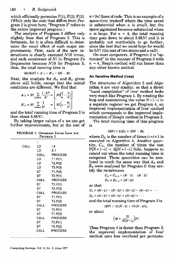
which efficiently permutes P[1], P[2], P[3]. (While only the code that differs from Pro- gram 2 is given here, '<Program 3" refers to the entire improved program.)
The analysis of Program 3 differs only slightly from that of Program 2. This is fortunate, for it is often difficult to deter- mine the exact effect of such major im- provements. First, each of the new in- structions is clearly executed N!/6 times, and each occurrence of N! in Program 2's frequencies becomes N!/6 for Program 3; thus, the total running time is
( 5 0 / 6 ) N ! + A ' N + B ' N + 6 N - 20.
Next, the analysis for AN and BN given above still holds, except that the initial conditions are different. We find that
A'N ' i ~ N k! =
and the total rum~Jng time of Program 3 is then about 8.88N!.
By taking larger values of n we can get further improvements, but at the cost of
P R O G R A M 3. OPTIMIZED INNER LOOP FOR PROGRAM 2
CALL LD 1,4 LD X,1 CALL PROCESS LD T1 ,P(1) LD T2,P(2) LD T3,P(3) ST T1 ,P(2) ST T2,P(1) CALL PROCESS ST T3,P(1) ST T2,P(3) CALL PROCESS ST T1 ,P(1) ST T3,P(2) CALL PROCESS ST T2,P(1) ST T1 ,P(3) CALL PROCESS ST T3,P(1) ST T2,P(2) CALL PROCESS
n+3n! lines of code. This is an example of a space-time tradeoff where the time saved is substantial when n is small, but the space f, o2_sumed becomes substantial when n is large. For n = 4, the total running time goes down to about 5.88N! and it is probably not worthwhile to go further, since the best that we could hope for would be 5N! (the cost of two stores and a call).
On most computers, if Program 2 is "op- timized" in the manner of Program 3 with n = 4, Heap's method will run faster than any other known method.
An Iterative Method (Ives)
The structures of Algorithm 2 and Algo- r i thm 4 are very similar, so that a direct "hand compilation" of Ives' method looks very much like Program 1. By rotating the loop and maintaining the value N + l - i in a separate register we get Program 4, an improved implementation of Ives' method which corresponds to the improved imple- mentation of Heap's method in Program 2.
The total running time of this program is
18N! + 21D N + 1 0 N - 25,
where DN is the number of times i: =i + 1 is executed in Algorithm 4. Another quan- tity, CN, the number of times the test P [ N + I - i ] = Q [ N + I - i ] fails, happens to cancel out when the total running time is computed. These quantities can be ana- lyzed in much the same way that AN and BN were analyzed for Program 2: they sat- isfy the recurrences
CN = C~v-2 + ( N - l ) ! - ( N - 2 ) v
DN = D1v-2 + ( N - 2 ) !
so that CN = ( N - l ) ! - ( N - 2 ) ! + ( N - 3 ) ! - ( N - 4 ) ! + " "
DN = ( N - 2 ) I + ( N - 4 ) ! + ( N - 6 ) ! + • • •
and the total running time of Program 2 is 18N! + 2 1 ( N - 2 ) + O ( ( N - 4 ) ! ) ,
or about
(18'+ 21 ~N, N(N- i) ]-"
Thus Program 4 is faster than Program 2: the improved implementation of Ives' method uses less overhead per permuta-
C o m p u t i n g Surveys , Vol 9, No 2, J u n e 1977
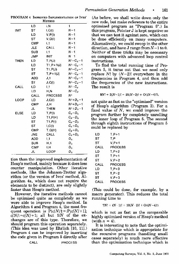
Permutation Generation Methods
P R O G R A M 4 IMPROVED IMPLEMENTATION OF IVES'
INIT
THEN
CALL
LOOP
METHOD
ELSE
LD I,N 1 ST I,C(I) N-1 LD V,P(I) N-1 ST V,Q(I) N-1 CMP 1,1 N-1 JLE CALL N-1 SUB 1,1 N-1 JMP INIT N-1 LD T,P(J) N I -CN- 1 LD T1 ,P+I(J) NI-CN-1 ST T1 ,P(J) NI-CN-1 ST T,P+I(J) NI-C~-I ADD J,1 NI-C~,-1 ST J,C(I) Nt-C~-I LD 1,1 N I-C~ LD H,N Nw-C~ CALL PROCESS NI LD J,C(I) Nm+DN-1 CMP J,H NS+DN-1 JL THEN NI+DN-1 LD T,P(I) CN+D,~ LD T1 ,P(H) CN+D~ ST T1 ,P(I) C,v+D~ ST I,C(I) C~+D~ CMP T,Q(H) C~+DN JNE CALL CN+DN ADD 1,1 D~ SUB H,1 DN CMP I,H DN JL LOOP D~
tion than the improved implementation of Heap's method, mainly because it does less counter manipulation. Other iterative methods, like the Johnson-Trotter algo- ri thm (or the version of Ives' method, Al- gorithm 4a, which does not require the elements to be distinct), are only slightly faster than Heap's method.
However, the iterative methods cannot be optimized quite as completely as we were able to improve Heap's method. In Algorithm 4 and Program 4, the most fre- quent operation is P[c[N]]:=:P[c[N]+I]; c[N]:=c[N]+l; all but 1IN of the ex- changes are of this type. Therefore, we should program this operation separately. (This idea was used by Ehrlich [10, 11].) Program 4 can be improved by inserting the code given in Program 5 directly after
CALL PROCESS
• 1 6 1
(As before, we shall write down only the new code, but make reference to the entire optimized program as "Program 5".) In this program, Pointer J is kept negative so that we can test it against zero, which can be done efficiently on many computers. Alternatively, we could sweep in the other direction, and have J range from N - 1 to 0. Neither of these tricks may be necessary on computers with advanced loop control instructions.
To find the total running time of Pro- gram 5, it turns out that we need only replace N! by (N-2)! everywhere in the frequencies in Program 4, and then add the frequencies of the new instructions. The result is
9N! + 2 ( N - l ) ! + 18(N-2) ! + O( (N-4) ! ) ,
not quite as fast as the "optimized" version of Heap's algorithm (Program 3). For a fixed value of N, we could improve the program further by completely unrolling the inner loop of Program 5. The second through eighth instructions of Program 5 could be replaced by
LD T,P+I ST T,P ST V,P+I CALL PROCESS LD T,P+2 ST T,P+I ST V,P+2 CALL PROCESS LD T,P+3 ST T,P+2 ST V,P+3 CALL PROCESS
(This could be done, for example, by a macro generator). This reduces the total running time to
7N! + ( N - l ) ! + 18(N-2) ! + O( (N-4 ) ! )
which is not as fast as the comparable highly optimized version of Heap's method (with n = 4).
It is interesting to note that the optimi- zation technique which is appropriate for the recursive programs (handling small cases separately) is much more effective than the optimization technique which is
Computing Surveys, Vol. 9, No. 2, June 1977
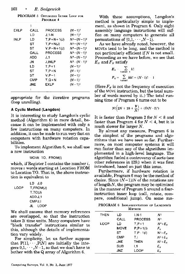
162 • R. Sedgewick
PROGRAM 5 OPTIMIZED INNER LOOP FOR PROGRAM 4
EXLP
INLP
CALL PROCESS (N-1)I LD J,1-N (N-1)v LD T,P+N+I(J) NI-(N-1)I ST T,P+N(J) NI-(N-1)v ST V,P+N+I(J) NV-(N-1)l CALL PROCESS NV-(N-1) I ADD J,1 NV-(N-1)~ JN J,INLP NI-(N-1)v LD T,P+I (N-1)~ ST T,P+N (N-1)v ST V,P+I (N-1)~ CMP T,Q+N (N-1)l JNE EXLP (N-1)l
appropriate for the iterative programs (loop unrolling).
A Cyclic Method (Langdon) It is interesting to study Langdon's cyclic method (Algorithm 6) in more detail, be- cause it can be implemented with only a few instructions on many computers. In addition, it can be made to run very fast on computers with hardware rotation capa- bilities.
To implement Algorithm 6, we shall use a new instruction
MOVE TO, FROM(I)
which, if Register I contains the number i, moves ~ words starting at Location FROM to Location TO. That is, the above instruc- tion is equivalent to
LD J,0 LOOP T,FROM(J)
T,TO(J) ADD J,1 CMPJ,I JL LOOP
We shall assume that memory references are overlapped, so that the instruction takes 2i time units. Many computers have "block transfer" instructions similar to this, although the details of implementa- tion vary widely.
For simplicity, let us further suppose that PI l l , . - .,P[N] are initially the inte- gers 0,1,. • • , N - l , so that we don't have to bother with the Q array of Algorithm 6.
With these assumptions, Langdon's method is particularly simple to imple- ment, as shown in Program 6. Only eight assembly language instructions will suf- fice on many computers to generate all permutations of {0,1,. • • , N - 1}.
As we have already noted, however, the MOVEs tend to be long, and the method is not particularly efficient i fN is not small. Proceeding as we have before, we see that EN and FN satisfy
EN = ~ k! l~k'~N--1
FN= ~ k k ! = ( N + l ) ! - 1 l ~ k ~ N
(Here FN is not the frequency of execution of the MOVE instruction, but the total num- ber of words moved by it.) The total run- ning time of Program 6 turns out to be
N , ( 2 N + 1 0 + 9 ) + ( O ( N - 2 ) ')
It is faster than Program 2 for N < 8 and faster than Program 4 for N < 4, but it is much slower for larger N.
By almost any measure, Program 6 is the simplest of the programs and algo- ri thms that we have seen so far. Further- more, on most computer systems it will run faster than any of the algorithms im- plemented in a high-level language. The algorithm fueled a controversy of sorts (see other references in [25]) when it was first introduced, based on just this issue.
Furthermore, if hardware rotation is available, Program 6 may be the method of choice. Since (N-1)/N of the rotations are of length N, the program may be optimized in the manner of Program 5 around a four- instruction inner loop (call, rotate, com- pare, conditional jump). On some ma-
PROGRAM 6 IMPLEMENTATION OF LANGDON'S METHOD
THEN
LOOP
LD I,N-1 NI CALL PROCESS NI LD T,P+I NV+E~ MOVE P,P+I(I) F~ ST T,P+I(I) NV+E~ CMP T,I NI+E N JNE THEN NI+EN SUB 1,1 E~ JNZ LOOP E~
Computing Surveys, Vol 9, No 2, June 1977
Permutation Generation Methods • 163
chines, the rotate might be performed in, say, two time units (for example, if paral- lelism were available, or if P were main- tained in registers), which would lead to a total time of 5N! + O((N-1)!). We have only sketched details here because the is- sues are so machine-dependent: the ob- vious point is that exotic hardware fea- tures can have drastic effects upon the choice of algorithm.
CONCLUSION
The remarkable similarity of the many permutation enumeration algorithms which have been published has made it possible for us to draw some very definite conclusions regarding their performance. In Section 1, we saw that the method given by Heap is slightly simpler (and therefore slightly more efficient) than the methods of Wells and Boothroyd, and that the method given by Ives is simpler and more efficient than the methods of Johnson and Trotter (and Ehrlich). In Section 2, we found that the cyclic and lexicographic al- gorithms will not compete with these, ex- cept possibly for Langdon's method, which avoids some of the overhead in the control structure inherent in the methods. By carefully implementing these algorithms in Section 3 and applying standard code optimization techniques, we found that Heap's method will run fastest on most computers, since it can be coded so that most permutations are generated with only two store instructions.
However, as discussed in the Introduc- tion, our accomplishments must be kept in perspective. An assembly-language imple- mentation such as Program 3 may run 50 to 100 times faster than the best previously published algorithms (in high-level lan- guages) on most computer systems, but this means merely that we can now gener- ate all permutations of 12 elements in one hour of computer time, where before we could not get t oN = 11. On the other hand, if we happen to be interested only in all permutations of 10 elements, we can now get them in only 15 seconds, rather than 15 minutes.
The problem of comparing different al- gorithms for the same task arises again
and again in computer science, because new algorithms (and new methods of ex- pressing algorithms) are constantly being developed. Normally, the kind of detailed analysis and careful implementation done in this paper is reserved for the most im- portant algorithms. But permutation gen- eration nicely illustrates the important is- sues. An appropriate choice between algo- rithms for other problems can be made by studying their structure, implementation, analysis, and %ptimization" as we have done for permutation generation.
ACKNOWLEDGMENTS
Thanks are due to P Flanagan, who implemented and checked many of the algomthms and programs on a real computer. Also, I must thank the many authors listed below for providmg me with such a wealth of maternal, and I must apologize to those whose work I may have misunderstood or misrepre- sented. Finally, the editor, P. J. Denning, must be thanked for his many comments and suggestmns for improving the readability of the manuscmpt.
REFERENCES
[1] BOOTI~OYD, J "PERM (Algorithm 6)," Com- puter Bullet in 9, 3 (Dec. 1965), 104
[2] BOOTHROVD, J. "Permutation of the elements of a vector (Algomthm 29)"; and "Fast permu- tation of the elements of a vector (Algorithm 30)," Computer J. 10 (1967), 310-312.
[3] BaATLEY, P "Permutations with repetitious (Algomthm 306)," Comm A C M 1O, 7 (July 1967), 450
[4] Cove, YOU, R R.; AND SULLrVAN, J. G. "Permutahon (Algorithm 71)," Comm. A C M 4, 11 (Nov 1961), 497.
[5] D~,aSHOWITZ, N. "A simplified loop-free algo- ri thm for generating permutatlous," B I T 15 (1975), 158-164.
[6] DIJKSTRA, E W A dzsc~pllne of program- m~ng, Prentice-Hall, Englewood Cliffs, N J ,, 1976.
[7] DZg~STaA, E. W "On a gauntlet thrown by David Gries," Acta Informat~ca 6, 4 (1976), 357.
[8] DURSTENFELD, R. "Random permutation (AI- gomthm 235)," Comm. A C M 7, 7 (July 1964), 420.
[9] EAVES, B. C "Permute (Algorithm 130)," Comm. A C M 5, 11 (Nov. 1962), 551 (See also: remarks by R. J. Ord-Smlth m Comm A C M 10, 7 (July, 1967), 452-3 )
[10] EHRLICH, G. "Loopless algomthms for gener- atmjg permutations, combinations and other combinatorial configurations," J A C M 20, 3 (July 1973), 500-513.
[11] EHRLICH, G "Four combmatomal algomthms (Algomthm 466)," Comm A C M 16, 11 (Nov 1973), 690-691.
Computing Surveys, Vol 9, No 2, June 1977
164 • R . Sedgewick
[12] EWN, S. Algortthmtc combtnatortcs, Macmil- lan, Inc., N.Y., 1973.
[13] FIKE, C T. "A permutation generation method," Computer J 18, 1 (Feb. 1975), 21-22.
[14] FISCHER, L. L.; AND KRAUSE, K. C , Lehr- buch der Combtnattonslehre und der Artthme- tzk, Dresden, 1812
[15] HALL, M.; ANDKNUTH, D.E. "Combinatorial analysis and computers," Amertcan Math. Monthly 72, 2 (Feb. 1965, Part II), 21-28.
[16] HEAl', B R. "Permutations by Inter- changes," Computer J. 6 (1963), 293-4.
[17] HOWELL, J R. "Generation of permutations by adchhon,"Math. Comp 16 (1962), 243-44
[18] HOWELL, J . R . "Permutation generater (Al- gorithm 87)," Comm. ACM 5, 4 (April 1962), 209. (See also: remarks by R. J. Ord-Smith in Comm ACM 10, 7 (July 1967), 452-3.)
[19] IvEs, F.M. "Permutation enumeration: four new permutatmn algorithms," Comm. ACM 19, 2 (Feb. 1976), 68-72.
[20] JOHNSON, S.M. "Generatlonofpermutations by adjacent transposition," Math. Comp. 17 (1963), 282-285.
[21] KNUTH, D.E. "Fundamental algorithms," in The art of computer pro~.rammzng 1, Addison- Wesley, Co., inc., Reading, Mass., 1968.
[22] KNUTH, D.E. "Seminumerlcal algorithms," m The art ofcom~uter programming 2, Addi- son-Wesley, Co., inc., Reading, Mass., 1969.
[23] KNUTH, D. E "Sorting and searching," in The art of computer programmtng 3, Addison- Wesley, Co., Inc, Reading, Mass, 1972
[24] KNUTH, D. E. "St,ru, ctured programming with go to statements, ' Computing Surveys 6, 4 (Dec. 1974), 261-301.
[25] LANaDON, G. G., Jr., "An algorithm for gen- erating permutations," Comm. ACM 10, 5 (May 1967), 298-9. (See also. letters by R. J. Ord-Smith in Comm. ACM 10, 11 (Nov. 1967), 684; by B. E. Rodden m Comm. ACM 11, 3 (March 1968), 150; CR Rev. 13,891, Computing Reviews 9, 3 (March 1968), and letter by Lang- don inComm. ACM 11, 6 (June 1968), 392.)
[26] LEH~R, D H. "Teaching combinatorial tricks to a computer," in Proc. of Symposlum Appl. Math ,Combtnatortal Analysis, Vol. 10, American Mathematical Society, Providence, R.I , 1960, 179-193.
[27] LEHMER, D.H. "The machine tools of combi- natemcs," m Applied comb~natortal mathe- matws (E. F. Beckenbach, [Ed.]), John Wiley, & Sons, Inc., N Y, 1964
[28] L~.mvi~.R, D.H. "Permutation by adjacent in- terchanges," Amerwan Math. Monthly 72, 2 (Feb. 1965, Part II), 36-46.
[29] Om)-SMITH, R J. "Generation of permuta- tion sequences Part 1," Computer J. 13, 3 (March 1970), 152-155.
[30] OaD-SMITH, R. J. "Generation of permuta- tion sequences: Part 2," Computer J. 14, 2 (May 1971), 136-139.
[31] ORD-SMITH, R. J. "Generation of permuta- tions in psoudo-lexicographic order (Algo- rithm 308)," Comm ACM 10, 7 (July 1967),
452 (See also: remarks in Comm ACM 12, 11 (Nov 1969), 638.)
[32] Om)-SMITH, R J "Generation of permuta- tions m lexicographlc order (Algorithm 323)," Comm. ACM 11, 2 (Feb. 1968), 117 (See also: certification by I. M. Leltch in Comm ACM 12, 9 (Sept. 1969), 512.)
[33] PECK, J E. L; AND SCHRACK, G F "Permute (Algorithm 86)," Comm. ACM 5, 4 (April 1962), 208.
[34] PHmLmS, J. P .N . "Permutation of the ele- ments of a vector in lexicographic order (Algo- rithm 28)," Computer J. 1O (1967), 310-311
[35] PLESZCZYNSKL S. "On the generation of per- mutations," Informatmn Processtng Letters 3, 6 (July 1975), 180-183.
[36] RIORDAN, J. An ~ntroductton to comb~nato- rtal analysts, John Wiley & Sons, Inc., N.Y., 1958.
[37] ROHL, J .S. , "Programming improvements to Fike's algorithm for generating permuta- tions," Computer J. 19, 2 (May 1976), 156
[38] ROBXNSON, C. L. "Permutation (Algorithm 317)," Comm. ACM 10, 11 (Nov. 1967), 729.
[39] SAG, T.W. "Permutations of a set with repe- titions (Algorithm 242)," Comm ACM 7, 10 (Oct 1964), 585.
[40] SCHRAK, G. F , AND SHIMRAT, M "Permutation in lexicographlc order (Algo- rithm 102)," Comm. ACM 5, 6 (June 1962), 346. (See also: remarks by R J Ord-Smith in Comm ACM 10, 7 (July 1967), 452-3.)
[41] SHEN, M.-K "On the generation ofpermuta- tlons and combinations," BIT 2 (1962), 228- 231
[42] SHEN, M -K "Generation ofpermutations in lexicographic order (Algorithm 202)," Comm ACM 6, 9 (Sept. 1963), 517. (See also: remarks by R. J. Ord-Snnth in Comm. ACM 10, 7 (July 1967), 452-3.)
[43] SLOANE, N. J. A. A handbook of tnteger se- quences, Academic Press, Inc , N Y, 1973
[44] TOMPKIN8, C. "Machine attacks on problems whoso variables are permutations," in Proc Symposium zn Appl. Math., Numerwal Analy- sts, Vol 6, McGraw-Hill, Inc., N.Y., 1956, 195-211
[45] TROTTER, H. F. "Perm (Algorithm 115)," Comm. ACM 5, 8 (August 1962), 434-435.
[46] WAL~R, R. J "An enumerative technique for a class of combinatorial problems," in Proc Symposium in Appl. Math, Combtnatorial Analysts, Vol. 10, American Mathematical So- ciety, Providence, R.I , 1960, 91
[47] WZLLS, M. B "Generation of permutations by transposition," Math Comp 15 (1961), 192- 195.
[48] WELLS, M. B. Elements of combtnatortal computtng, Pergamon Press, Elmsford, N.Y., 1971.
[49] WHITEHEAD, E. G. Combinatorial algo- rithms. (Notes by C. Frankfeldt and A. E. Kaplan) Courant Institute, New York Univ., 1973, 11-17.
Computlng Surveys, Vol 9, No 2, June 1977


![Design - Princeton Universityrblee/ELE572Papers/Fall04Readings/Shifter... · This pap er examines design alternativ es for barrel shifters that ... [16], sev eral 32-bit barrel shifters](https://img.dokumen.tips/doc/110x75/5aa5a5fe7f8b9afa758d8786/design-princeton-rbleeele572papersfall04readingsshifterthis-pap-er-examines.jpg)