Final Report

Performance of the HVAC Systems

at the ASHRAE Headquarters Building

Jeffrey D. Spitler and Laura E. Southard, Oklahoma State University

Xiaobing Liu, Oak Ridge National Laboratory

September 30, 2014

This report was the result of independent study by Dr. Jeff Spitler and Laura E. Southard, Oklahoma State University, and Dr. Xiaobing Liu, Oak Ridge National Laboratory—with the gracious cooperation of the American Society of Heating, Refrigeration and Air-conditioning Engineers (ASHRAE).

Acknowledgments The researchers thank ASHRAE for making comprehensive comparison data available from their ground-source (geothermal) heat pump and variable refrigerant flow heating and cooling systems at the ASHRAE headquarters building in Atlanta, Georgia. Without ASHRAE’s assistance, this report would not have been possible. We also extend special thanks to Mike Vaughn, Manager of Research and Technical Services at ASHRAE, for helping us with access to the data and to the building during our site visit. The project was funded by GEO—The Geothermal Exchange Organization, with additional support from the Southern Company, which also provided a power engineer to assist with onsite measurements. Dr. Liu's time was also supported by the US-China Clean Energy Research Center for Building Energy Efficiency (CERC-BEE).

GEO – The Geothermal Exchange Organization 312 South 4th Street Springfield, IL 62701 Phone (888) 255-4436 Email GEO@geoexchange.org Website www.geoexchange.org

Table of Contents Executive Summary 1 Chapter 1 – Introduction 8 1.1 Literature review 8 1.2 Building description 8 1.3 HVAC systems description 12 1.3.1 VRF system 12 1.3.2 GSHP system 14 1.3.3 DOAS system 16 1.4 Instrumentation description and data acquisition 20 1.5 Objectives 21 Chapter 2 – Overall Energy Use 22 2.1 Floor areas 23 2.2 System energy use dependence on ambient dry bulb temperature 25 2.3 Operational conditions and efficiencies 28 2.4 Control strategies 31 2.4.1 Mild weather example 32 2.4.2 Warm weather example 34 2.5 Simultaneous heating and cooling 36 Chapter 3 – Methodology for Estimating Heating and Cooling Provided 40 3.1 Performance curve models 41 3.1.1 Mixed air humidity estimation 42 3.1.2 Validation of TTH038 cooling mode power input model 43 3.1.3 Performance degradation at cycle onset 45 3.2 Ground loop measurements with modeled power estimates 47 3.3 Air side measurements 49 3.3.1 Discharge air humidity estimation 50 3.3.2 VRF mixed air temperature estimation 51 3.3.3 VRF mixed air and discharge air humidity estimation 51 3.3.4 VRF air flow rates 52 3.3.5 Uncertainty Analysis 53 Chapter 4 – Results 56 4.1 Method validation using zone 215B data 56 4.2 Estimates of GSHP system cooling and heating provided 59 4.3 Estimates of VRF system cooling and heating provided 63 4.4 Estimate of DOAS system cooling provided 65 4.5 Performance metrics 66 Chapter 5 – GSHP System Energy Analysis 70 5.1 Heat pump energy 70 5.2 Standby energy use 70

5.3 Circulation pump energy use 71 5.4 Ventilation blower energy use 75 5.5 Complete energy analysis 75 Chapter 6 – Conclusions 79 Chapter 7 – Recommendations 81 References 84 Appendix A – Collected data points 86 Appendix B – Heat pump performance curve model coefficients 100 Appendix C – Power monitoring data 103

All photographs in this document appear courtesy of Petr Konecny

1

Executive Summary

In 2008, the ASHRAE Headquarters Building in Atlanta underwent major renovation. The two-story, 31,000 sq. ft. building was switched to an open plan configuration, an addition was constructed, and new state-of-the art HVAC systems were added. A ground source heat pump system now serves the second floor and a variable refrigerant flow system serves the first floor. In addition, a dedicated outdoor air system provides filtered and conditioned outdoor air to maintain indoor air quality on both floors. Intended for use as a “living laboratory”, the building is extensively instrumented with about 1600 data points being measured and recorded. The focus of this project was comparison of the performance of the ground source heat pump system and the variable refrigerant flow system. Despite the availability of 1600 measurements, many desired measurements, especially the heating and cooling provided by each system, are not available. Therefore much of the work involved analysis of the data, post-processing of the data to estimate quantities such as heating and cooling provided, and uncertainty analysis to characterize the accuracy of the results. In addition to this summary, this report consists of a master’s thesis by Laura Southard, Performance of the HVAC Systems at the ASHRAE Headquarters Building, which provides the most detailed account of the work. Also available are two papers describing the work that have been published in the ASHRAE Journal. They provide a shorter synopsis of the findings:

• Southard, L.E., X. Liu, J.D. Spitler. 2014. “Performance of HVAC Systems at ASHRAE HQ – Part 1.” ASHRAE Journal. September 2014, 56(9):14-24. Link to it online here.*

• Southard, L.E., X. Liu, J.D. Spitler. 2014. “Performance of HVAC Systems at ASHRAE HQ – Part 2.” ASHRAE Journal. December 2014, 56(12): 12-23. Link to it online here.*

*ASHRAE stipulates that anyone publishing links to their Journal articles include the following statement: “Use of the data published in ASHRAE Journal regarding performance of ASHRAE International Headquarters may not state nor imply that ASHRAE has endorsed, recommended, or certified any equipment or service used at ASHRAE International Headquarters.” The key findings from this work can be divided into two parts. First, conclusions that can be drawn from the measured data prior to determining the heating and cooling provided:

• For the two-year time span of this study, the VRF system used 98% more total energy than the GSHP system, 41% more in the summer cooling season (May - September) and 172% more in the winter and shoulder seasons (October – April).

• The DOAS system used more power than the either the VRF or GSHP system. • Although the renovation added a large conference room to the first floor, the area

served by the VRV-III heat recovery system is only about 11% larger than the area

2

served by the GSHP system. The difference in floor area does not account for the difference in energy use. On a square foot basis the VRF system used 79% more total energy than the GSHP system over the two year study period. Figure 1 shows the monthly energy usage by both systems on a per square foot basis, illustrating that month in and month out, the GSHP system uses less energy than the VRF system. Figure 2 shows the average power usage of the two systems per square foot.

Figure 1. Normalized monthly energy use per square foot

Figure 2. Average power use vs. ambient temperature

0.00

0.05

0.10

0.15

0.20

0.25

0.30

0.35

Mon

thly

Ene

rgy

Use

, kW

h/ft

2

GSHP VRF

3

As illustrated in Figure 2, the GSHP system has lower energy usage at all outdoor air temperatures. The conclusion from our research is that there are two reasons for this:

• At both ends of the temperature range, the GSHP system has better operational

efficiencies due to the thermodynamic advantages of rejecting heat to or extracting heat from the ground rather than the air.

• The control strategies used with the VRF system that involve tightly controlled single set point temperatures for adjacent zones in an open office environment create situations where adjacent zones in the building are being simultaneously heated and cooled. This shows up in the middle temperature ranges where less heating or cooling is needed. This can also be illustrated with Figures 3 and 4 which show the contributions of heating and cooling to the electrical energy consumption of both systems. As can be seen, at mid-range temperatures, e.g. 55°F, the VRF system has both heating and cooling energy consumption that is considerably higher than the total GSHP system energy consumption.

• Higher outdoor air flow rates for the first floor decreased the cooling demands and increased the heating demands for the VRF system. Also, the high DOAS flow rates and tightly controlled zone temperatures led to heating operation in warm weather on the first floor.

• Changing the loop differential pressure set point from 20 psi to 8 psi caused the pumping power to drop from 17% of the total GSHP system power to 7%.

Figure 3. Contributions of heating and cooling to VRF system power use

0

0.2

0.4

0.6

0.8

1

1.2

1.4

1.6

1.8

2

17 25 30 35 40 45 50 55 60 65 70 75 80 85 90 95 100

Aver

age

VRF

Pow

er U

se, W

/ft2

Ambient Dry Bulb Temperature, °F

VRF Heating Cooling

4

Figure 4. Contributions of heating and cooling to GSHP system power use In order to evaluate system performance, the amount of heating and cooling provided must be determined. Determining the amount of heating and cooling provided necessarily involve some approximations, for which the uncertainty has been estimated. Several different approaches were used to determine the heating and cooling provided to the building. Of these, determination of the cooling and heating provided by utilizing measured temperatures and air flow rates measured at commissioning (“air side analysis”) had the highest accuracy – the uncertainty is +14%/-11% for cooling provided by the GSHP system and ±7% for heating provided by the GSHP system. For the VRF system, the uncertainty is ±5% for cooling and ±4% for heating. This analysis can be applied to the GSHP system for the entire two-year period between July 2011 and June 2013. It can only be applied to the VRF system from July 2011 through March 2012 because the control boards in the FCUs were changed out, changing the air flow rates, which were not subsequently measured. The heating and cooling provided by the two systems is summarized in Figures 5 and 6. In general, the VRF system provides more heating in the winter than the GSHP system; this is largely due to the higher flow of cool air coming into the first floor from the DOAS. Conversely, the GSHP system provides more cooling than the VRF system in summer; this is due to the different DOAS flows and the fact that the GSHP system has higher envelope loads because of the roof.

00.20.40.60.8

11.21.41.61.8

2

17 25 30 35 40 45 50 55 60 65 70 75 80 85 90 95 100

Aver

age

GSH

P Po

wer

Use

, W/f

t2

Ambient Dry Bulb Temperature, °F

GSHP Heating Cooling Unallocated

5

Figure 5. Monthly heating provided

Figure 6. Monthly cooling provided Knowing the electrical energy used each month, and the monthly heating and cooling provided, COP and EER for both systems can be determined. These are shown in Figures 7 and 8. Even considering the uncertainties, the GSHP system has notably higher EERs and COPs. Conclusions that can be drawn from the air-side analysis include:

• Power measurements and estimates of the heating and cooling provided based on air side measurements show that GSHP system cooling EERs are 15-16 in the summer and system heating COPs are 3-4 in the winter. These system COPs and EERs include

0.00

0.10

0.20

0.30

0.40

0.50

0.60

Heat

ing

Prov

ided

, kW

h/ft

2

GSHP

VRF

0.0

0.2

0.4

0.6

0.8

1.0

1.2

1.4

Cool

ing

Prov

ided

, kW

h/ft

2

GSHP

VRF

6

all energy use by the GSHP system, including pumping, fan power in ventilation mode and standby power consumption of the heat pump control boards, BAS control panel and circulation pump VFDs.

• For July – September, 2011 the GSHP system cooling EER was 15.6 +2.2/-1.7; the VRF system cooling EER was 10.7 ±0.5.

• For the winter of 2011-2012, the GSHP system heating COP was 3.3±0.2 and the VRF system heating COP was 2.0±0.1.

• For the summer of 2012, the VRF COPs could not be determined based on air side measurements, but the GSHP system cooling EER was 15.8+2.2/-1.7.

Figure 7. Estimated monthly system heating COP

Figure 8. Estimated monthly system cooling EER

0.0

1.0

2.0

3.0

4.0

5.0

6.0

Heat

ing

Syst

em C

OP

GSHP VRF

0

2

4

6

8

10

12

14

16

18

20

Cool

ing

Syst

em E

ER

GSHP VRF

7

As demonstrated several ways during the project, the VRF system performance appears to be hampered by unnecessary simultaneous heating and cooling in adjacent zones. As the system has been operating more than five years this way, we may speculate that the simultaneous heating and cooling problem is not amenable to a quick and easy fix. This problem particularly degrades performance at moderate temperature conditions when heating and cooling loads should be very small. It has also been shown that both low and high outdoor air temperatures when heating and cooling dominate, respectively, the GSHP system gives better performance than the VRF system.

8

Chapter 1

Introduction The purpose of this study is to compare the performance of the ground source heat pump (GSHP) and variable refrigerant flow (VRF) systems that are installed at the ASHRAE headquarters building in Atlanta, Georgia. Most buildings have only one primary type of HVAC system installed for the property. Thus trying to compare different types of HVAC systems typically involves making adjustments for the differences in the specific details of different installations. Having two types of systems installed for different areas of the same building gives a unique opportunity to eliminate many of the variables associated with building construction, space utilization and location. 1.1 Literature review GSHP and VRF systems installed in an operational environment seldom have enough instrumentation to perform a detailed evaluation of the performance of the systems. Evaluations of the field performance of a GSHP system are available for office buildings in China (Li, et al,. 2009, Zhao, et al., 2005), an industrial greenhouse in Japan (Li, et al., 2013) and single family residences in Germany (Loose, et al., 2011), Connecticut, Virginia and Wisconsin (Puttagunta, et al., 2010). Evaluations of the field performance of a VRF system are available for 4-room office suites in China (Zhang, et al., 2011) and in Maryland (Aynor, et al., 2011, Kwon, et al., 2012, Kwon, et al. 2014). Although simulation studies comparing VRF and GSHP system performance for the same building are available (Liu and Hong, 2010, Wang, 2014), actual installed performance data for both types of systems in one building has not been readily available before. 1.2 Building description The ASHRAE headquarters building is located in Atlanta. The 2-story building was originally constructed as a 30,000-ft2 office building in 1965 and was purchased by ASHRAE in 1980 (Vaughn, 2014). The building underwent extensive renovations in 2007-2008, which included a 4,000-ft2 addition containing conference rooms, corridors and a vestibule on the first floor and a new stairwell. The original portion of the building envelope has a curtain wall construction with alternating sections of brick pilasters and windows, with spandrel glass above and below the windows (Spitler, 2010). The new addition has windows along the corridor and vestibule and solid walls around all three exterior sides of the conference room. For both brick and spandrel sections, the overall resistance of the walls is 13 h-ft2-°F/Btu. The building is built on a concrete slab with an overall resistance of 7 h-ft2-°F/Btu, and the roof has six inches of R-5 rigid foam core insulation between the metal deck and the membrane roofing material making the overall resistance of the roof 31 h-ft2-°F/Btu. The windows are double-gazed with ½–in. air space

9

between a ¼-in. bronze-tinted outdoor pane and a ¼-in. clear indoor pane. The windows are inoperable in aluminum frames with thermal breaks and have a normal SHGC of 0.49 and an overall combined U of 0.56 Btu/h-ft2-°F (ASHRAE, 2013).

Figure 1-1

Exterior of building showing alternating brick and spandrel sections

Figure 1-2

Exterior of the new addition

10

Individual workstations are arranged in an open-office layout with minimal perimeter offices and glass-walled cubicles to maximize outdoor views and daylight for the occupants. Interior lighting is controlled by a combination of photocells, occupant (CO2) sensors and schedules.

Figure 1-3

Open office floor plan with glass-walled cubicles and outdoor views

Throughout the building the thermostats have base set points which are set by the building automation system (BAS). The occupants can adjust the set points ±3°F to suit individual comfort levels.

Figure 1-4

Thermostat with locally adjustable setpoint

11

The roof of the original structure has a cool white reflective membrane, while the roof of the addition has a rooftop garden.

Figure 1-5 White roof membrane on original structure

Figure 1-6 Rooftop garden on new building addition

12

1.3 HVAC systems description One of the goals of the renovation was to create a living lab that could be used for research by ASHRAE and its members. As a part of this living lab concept, the building uses three separate HVAC systems – a variable refrigerant flow (VRF) system to provide heating and cooling to the first floor, a ground source heat pump (GSHP) system, primarily for spaces on the second floor, and a dedicated outdoor air system (DOAS), which supplies fresh air to both floors for ventilation. 1.3.1 VRF system The first floor is conditioned by five independent Daikin inverter-driven VRF systems. A 4-ton VRV-S system connected to a ducted fan coil unit (FCU) provides heating and cooling to the new vestibule, reception area and stairwell. Two 3-ton SkyAir VRF systems connected to ductless FCUs cool a computer equipment and server room. And two 14-ton VRV-III heat recovery type systems connected by a 3-pipe system to 22 ducted FCUs with a total of 35 ⅝ nominal tons of cooling capacity provide heating and cooling to the office areas and conference rooms on the first floor. Each of the 14-ton VRV-III heat recovery systems has two separate outdoor condensers: a 6-ton unit and an 8-ton unit. All five of the systems use HFC-410A refrigerant.

Figure 1-7 A 14-ton VRV-III heat recovery system outdoor units front elevation

13

Figure 1-8

A 14-ton VRV-III heat recovery system outdoor units rear elevation

Figure 1-9

One VRV-S and two SkyAir outdoor units

14

Daikin North America LLC provided engineering data, operation, installation and service manuals for all of the equipment models used in the ASHRAE headquarters building. During heating operation, VRF systems must occasionally switch to a defrost cycle. Defrost operation is described by the VRV-III product brochure (Daikin, 2013): “Each heat exchanger is defrosted by using heat transferred from one heat exchanger to the other in the outdoor unit.” The FCUs have two-speed fans that operate continuously at low speed for ventilation when the building is occupied. When heating or cooling is initiated, the fans switch to high speed operation for the duration of the cycle. The FCU fans operate at a constant air flow rate when the coils are on. 1.3.2 GSHP system The GSHP system includes 14 Climatemaster water-to-air heat pumps with a total nominal capacity of 31 ½ tons. Two ¾-ton Tranquility console units provide heating and cooling to both floors of the rear stairwell. Six 2-ton and six 3-ton Tranquility 27 series 2-stage heat pumps with electronically commutated motor (ECM) fans provide heating and cooling to the remainder of the second floor. All 14 of the heat pumps use HFC-410A refrigerant.

Figure 1-10 A ¾-ton Tranquility console heat pump

15

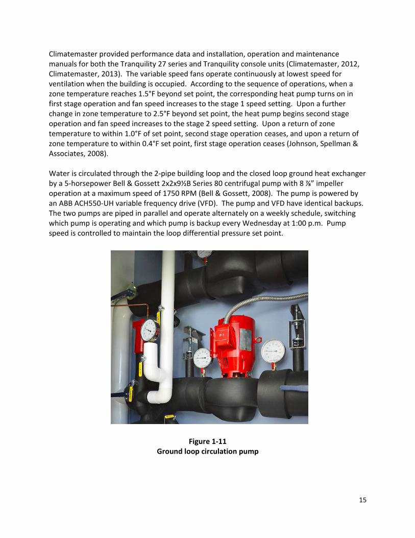
Climatemaster provided performance data and installation, operation and maintenance manuals for both the Tranquility 27 series and Tranquility console units (Climatemaster, 2012, Climatemaster, 2013). The variable speed fans operate continuously at lowest speed for ventilation when the building is occupied. According to the sequence of operations, when a zone temperature reaches 1.5°F beyond set point, the corresponding heat pump turns on in first stage operation and fan speed increases to the stage 1 speed setting. Upon a further change in zone temperature to 2.5°F beyond set point, the heat pump begins second stage operation and fan speed increases to the stage 2 speed setting. Upon a return of zone temperature to within 1.0°F of set point, second stage operation ceases, and upon a return of zone temperature to within 0.4°F set point, first stage operation ceases (Johnson, Spellman & Associates, 2008). Water is circulated through the 2-pipe building loop and the closed loop ground heat exchanger by a 5-horsepower Bell & Gossett 2x2x9½B Series 80 centrifugal pump with 8 ⅞” impeller operation at a maximum speed of 1750 RPM (Bell & Gossett, 2008). The pump is powered by an ABB ACH550-UH variable frequency drive (VFD). The pump and VFD have identical backups. The two pumps are piped in parallel and operate alternately on a weekly schedule, switching which pump is operating and which pump is backup every Wednesday at 1:00 p.m. Pump speed is controlled to maintain the loop differential pressure set point.

Figure 1-11

Ground loop circulation pump

16

Figure 1-12

Variable frequency drive for ground loop circulation pump The geothermal field lies under the parking lot and consists of twelve 400-foot deep vertical boreholes containing 1-¼” HDPE pipes in a single U-tube configuration. Design documents (Johnson Spellman & Associates, 2007) specified the use of thermally enhanced grout. The boreholes are in a 2 x 6 arrangement on 25-foot centers. Ewbank and Associates conducted an in-situ thermal conductivity test on February 3-6, 2008. Ewbank and Associates reported a deep earth temperature of 67.02°F with an earth thermal conductivity of 1.88 Btu/hr-ft-°F and a grout thermal conductivity of 0.98 Btu/hr-ft-°F (Ewbank and Associates, 2008). 1.3.3 DOAS system The DOAS system is a custom built unit manufactured by Trane that can provide up to 6000 CFM of outside air at 55°F with a 46°F dew point (Trane, 2007). The design conditions of the entering outside air are 82°F dry bulb and 77.1°F wet bulb. It includes dual stage air-to-air heat recovery desiccant wheels, variable speed supply and exhaust fans, and six staged DX condensing units with R-410A refrigerant. The total cooling capacity of the condensing units is 28.6 tons. Figure 1-13 shows a schematic diagram of the DOAS unit.

17

Figure 1-13

DOAS schematic diagram From ASHRAE National Headquarters BAS – Automated Logic Corporation

Figure 1-14

Custom built DOAS

18

Figure 1-15

Staged condensing units for the DOAS system

The air handler is connected to 24 variable air volume terminal boxes (VAV), 15 on the first floor and nine on the second floor. Five of the VAV units (for zones 135, 138, 217, 219 and 225) are controlled to maintain temperature set points for those zones. The remaining VAVs are controlled to maintain zone CO2 levels at 700 ppm above the outdoor CO2 level. The VAVs for zones 217 and 225 have electric reheat coils to provide heating to those zones (Johnson, Spellman & Associates, 2008). The DOAS maintains a slight positive pressure in the building, which minimizes infiltration. Ten of the 15 VAVs on the first floor provide fresh air directly to diffusers in the zones that they serve. The remaining five VAVs provide fresh air that mixes with return air entering the inlet of 14 of the FCUs. For the remaining eight FCUs, fresh air is not mixed with the return air. On the second floor four of the nine VAVs provide fresh air directly to the zones they serve while the remaining five VAVs provide fresh air that mixes with return air to the inlet of 11 of the GSHPs. For the remaining three GSHP units fresh air is not mixed with the return air (B.H.W Sheet Metal Company, 2008). Figures 1-16 and 1-17 show the arrangements of the zones on each floor.

19

Figure 1-16 First floor HVAC zones

From ASHRAE National Headquarters BAS – Automated Logic Corporation

Figure 1-17

Second floor HVAC zones From ASHRAE National Headquarters BAS – Automated Logic Corporation

20

1.4 Instrumentation description and data acquisition Another aspect of the living lab concept is the building automation system (BAS), which monitors information from over 1600 points on the zone conditions, equipment operations, and resource use. Measured data include space temperature, humidity, and CO2 concentration, individual unit operating status, operating mode, air flow rate, discharge air temperature and humidity, and energy use for a variety of subcategories. Information on the sensors that are installed in the building is in Table 1-1 (ALC Controls, 2008).

Table 1-1 Instrumentation details

Sensor Type Manufacturer Part Number Description Accuracy

Air temperature

BAPI ALC/10K-2-D-8”

Duct temperature

sensor

±0.2°C

Water temperature

BAPI ALC/10K-2-I-2”

Immersion temperature

sensor

±0.2°C

Air flow rate Ebtron Airflow measuring

station

±2% of reading

Water flow rate

Onicon F-1310 Dual turbine water flow meter

±2% of reading

Relative Humidity

BAPI ALC/H300 Humidity sensor, 3%

±3% RH

The data are stored at intervals ranging from 5 minutes to 1 hour and are accessible through an Internet portal. Historical data are available beginning in March 2010, although gaps of several days exist for four distinct periods between August 2010 and June 2011. The two-year time span of July 1, 2011 – June 30, 2013 was chosen for this study. Data for 559 data points were collected. A list of data points that were collected is in Appendix A. Data were acquired by logging into the BAS Internet portal, selecting a group of up to 16 points of interest and creating a trend graph of those points for a specific time period. Right clicking on the graph presents an option to copy the data presented in the trend graph to the clipboard. From there it was pasted into an Excel spreadsheet. For a set of several data points that are logged every 15 minutes, typically about six months of data can be captured without overflowing the clipboard capacity. While data points for flow rates, temperatures, and humidities are recorded every 15 minutes, data points for compressor start/stop, reversing valve position, and operating mode are recorded on change. Raw data was pre-processed by an Excel VBA program to add information

21

on operating mode, compressor status and reversing valve position to every line and to remove lines that did not contain temperature measurements. Some temperature and humidity data points are only recorded hourly, so pre-processing programs interpolated values for the quarter and half hour intervals. Power data are recorded every five minutes, so pre-processing selected only 15-minute data points for instantaneous matching with operating conditions. When pre-processing was completed, data files contained 70,168 lines of data (every 15 minutes for two years) for each relevant data point. Weather data points from the BAS system proved to be non-functional or inaccurate, so weather for 2011-2013 was purchased from White Box Technologies. The weather data files contain hourly measurements, so data that would be correlated to weather were again pre-processed to select only hourly data points. 1.5 Objectives The objectives of this work are fourfold:

1. To determine how much energy the VRF and GSHP systems used during the two-year study period.

2. To determine how much heating and cooling were provided by the VRF and GSHP systems during the two-year study period.

3. To compare the energy efficiency of the VRF and GSHP systems using appropriate performance metrics.

4. To determine the underlying reasons for differences in energy use and identify ways to improve the energy efficiency of both the VRF and GSHP systems.

22

Chapter 2

Overall Energy Use Metered energy use for each of the three HVAC systems was collected for the two-year study period. For the DOAS system, the metered energy use includes the power for all components of the system. Likewise, for the GSHP system, the metered energy use includes the power for all 14 heat pumps and for the water circulation pump. In contrast, the metered energy use for the VRF system does not include all of the equipment associated with the VRF system. It only includes the power for the two VRV-III heat recovery units and the 22 FCUs that are connected to them. The power for the two heat pumps that cool the computer equipment room and the heat pump that provides heating and cooling for the new vestibule and reception area is metered through a different subsystem that also includes all of the power for the servers and other equipment in the computer room. Figure 2-1 shows a month-by-month break down of the energy use of each HVAC system.

Figure 2-1 Total monthly energy use of each HVAC system

For the two-year study period, the DOAS system used a total of 112 MWh of electricity, the VRF system used 95 MWh, and the GSHP system used 48 MWh, which is slightly over half the energy used by the VRF system. In the summer cooling season (May – September), the VRF system used 41% more energy than the GSHP system, while the DOAS used more than both the VRF and GSHP system combined. In the winter and shoulder seasons (October – April), the VRF system used 2.7 times the energy that the GSHP system used, while the DOAS, which only heats air through the heat recovery wheels, used 1.1 times the energy that the GSHP system used.

02000400060008000

100001200014000160001800020000

Mon

thly

Ene

rgy

Use

, kW

h

GSHP VRF DOAS

23

Many factors affect the energy use of HVAC systems. Four factors have been identified as possible sources of the significant differences in energy use between the GSHP and VRF systems. They are:

1. The size of the floor area conditioned by each system. 2. The operating conditions of each system and the operational efficiency of each system

under the operating conditions. 3. The control strategies associated with each system. 4. The amount of heating and cooling provided to the area served by each system.

The contributions of each of the first three factors will be considered in this chapter. Different methods for estimating the heating and cooling provided to each floor will be explained in Chapter 3, and the resulting estimates obtained by each of the methods will be presented in Chapter 4. 2.1 Floor areas Since the renovation added a new entrance to the building and a new large conference room to the first floor, the first and second floors are no longer the same size. The total area of the first floor is now 18,536 ft2, while the area of the second floor is 15,248 ft2. However, a small zone (310 ft2) for the rear stairwell on the first floor is served by a heat pump, so the total floor area served by the heat pump system is 15,558 ft2. Also, the computer room (315 ft2) and the vestibule, reception area and front stairwell are served by the VRV-S and SkyAir heat pumps that are not included in the metered VRF system power data. Since the reception area is open to two corridors that are served by FCUs that are part of the VRV-III heat recovery system it is difficult to approximate the actual area conditioned by the VRV-S unit, but based on the locations of diffusers for this zone and the adjacent zones, the area served by the VRV-S unit is approximately 698 ft2. This makes the total floor area served by the metered VRF system 17,213 ft2. Thus the floor area served by the VRF system is only 11% greater than the area served by the GSHP system. Figure 2-2 is a floor plan of the first floor showing the areas that are not served by the metered VRF system.

24

Figure 2-2 Floor plan of the first floor showing areas not conditioned by metered VRF system

(Richard Wittschiebe Hand, 2007)

Figure 2-3 accounts for the differences in floor area served by showing the monthly energy use in kWh/ft2.

Figure 2-3 Monthly energy use on square foot basis

On a square foot basis, over the two-year time span, the GSHP system used 56% of the energy that the VRF system used.

0.00

0.05

0.10

0.15

0.20

0.25

0.30

0.35

Mon

thly

Ene

rgy

Use

, kW

h/ft

2

GSHP VRF

25

2.2 System energy use dependence on ambient dry bulb temperature Figure 2-3 shows the monthly energy use of each system on a square foot basis. The blue bars show that for the GSHP system, energy use peaks in the summer with smaller peaks in the winter, and lowest energy use in fall and spring, as expected. The red bars show that for the VRF system, energy use in the winter is almost as high as in the summer and monthly energy use remains above 0.16 kWh/ft2 year round. One of the standard methods used to model measured building energy use is the change-point regression model (Haberl, et al., 2003, Kissock, et al., 2002, Haberl and Cho, 2004). This method correlates energy use to ambient dry bulb temperature. The instantaneous VRF, GSHP and DOAS system power use in W/ft2 was matched to the corresponding ambient dry bulb temperature data from White Box Technologies. These data points were then filtered to include only the hours when the building was occupied (7 AM – 6 PM on work days). This resulted in a set of 6009 data points which were grouped in 1°F temperature bins. The average power use was calculated for each system for the set of data points in each temperature bin. Figure 2-4 shows the relationship between average power use and ambient dry bulb temperature for each of the three HVAC systems, and Figure 2-5 shows the number of data points that were averaged for each temperature bin.

Figure 2-4 Average power use vs. ambient dry bulb temperature

00.20.40.60.8

11.21.41.61.8

2

15 35 55 75 95

Aver

age

Pow

er U

se, W

/ft2

Ambient Dry Bulb Temperature, °F

GSHP VRF DOAS

26

Figure 2-5 Hours of power measurement data in each temperature bin

The data set of temperatures and corresponding power use for the VRF and GSHP systems were modeled with a 5-parameter change-point model (Haberl and Cho, 2004):

for T≤Th

for Th<T<Tc (2-1)

for T≥Tc

The temperatures and power use for the DOAS system was modeled with a 3-parameter change point model:

for T≤Tc (2-2)

for T>Tc

where E = measured instantaneous system power use T = ambient temperature Th = heating change-point temperature Tc = cooling change point temperature C = power use between the heating and cooling change points mh = slope that describes the linear dependence of power use on temperature below the heating change point mc = slope that describes the linear dependence of power use on temperature above the cooling change point

020406080

100120140160180200

17 24 28 32 36 40 44 48 52 56 60 64 68 72 76 80 84 88 92 96 100

Ambient Dry Bulb Temperature, °F

27

The models were implemented using Excel solver to determine the optimum values for each of the five parameters (C, Th, Tc, mh, and mc) by minimizing the sum of the errors squared. Figure 2-6 shows the resulting change-point model for each system and Table 2-1 gives the values of the model parameters for each system.

Figure 2-6 Average power use vs. ambient dry bulb temperature with change-point models

Table 2-1 Change point model parameters

System C, W/ft2 Th, °F Tc, °F mh, W/ft2-°F mc, W/ft2-°F

VRF 0.67 46.7 80.6 -0.039 0.026 GSHP 0.19 44.4 60.9 -0.017 0.014 DOAS 0.13 46.3 0.015

At ambient air temperatures near 100°F, the VRF system used 50% more power than the GSHP system. The power use of the VRF system decreased more sharply than the power use of the GSHP system as temperatures decreased until 81°F. At that temperature, the VRF system reached its minimum power usage (represented by the horizontal portion of the model) of about 0.67 W/ft2. Meanwhile the power use of the GSHP continued to decrease until 61°F. At that temperature it reached a minimum power use of 0.19 W/ft2, which is less than ⅓ of the minimum power use of the VRF system. The power use of both systems increases again once temperatures drop below the mid-40s °F, but the power use of the VRF system increases more sharply than the power use of the GSHP system. At temperatures between 25 and 63 °F the power use of the VRF system is three to four times the power use of the GSHP system.

00.20.40.60.8

11.21.41.61.8

2

15 35 55 75 95

Aver

age

Pow

er U

se, W

/ft2

Ambient Dry Bulb Temperature, °F

GSHP VRF DOAS

28

2.3 Operational conditions and efficiencies One of the primary differences between GSHP systems and VRF systems is the heat source or sink that heat is being extracted from or rejected to. GSHP systems extract heat from or reject heat to the ground, while VRF systems use air as the heat source or sink. As such, the ground loop water supply temperature and the ambient air temperature are the primary factors affecting the operational efficiency of each system. The hourly ground loop water supply and ambient air temperatures are plotted in Figure 2-7 for hours that the building is occupied, thus zone set points are at normal values and both HVAC systems are operating.

Figure 2-7 Ambient air and ground loop water supply temperatures during occupied hours

Figure 2-7 shows that the ground loop water supply temperatures are cooler in summer when heat is rejected and warmer in winter when heat is extracted, giving the GSHP system a thermodynamic advantage. Also, the differential between air and water temperatures is much greater in winter, giving the GSHP system a larger advantage in the winter. Equipment manufacturers make performance data available which give the equipment capacity and power input over a range of operating conditions. For the VRF system, equipment performance depends on the outdoor and indoor air dry bulb and wet bulb temperatures and the ratio of operating indoor FCU capacity to outdoor condenser capacity. For heat pumps, equipment performance depends on the entering air temperature and flow rate and entering water temperature and flow rate. Figures 2-8 through 2-11 show the manufacturers’ data for the expected performance of the VRF system and the GSHP equipment for cooling and heating over a range of source temperatures. The shaded area in these figures represents the range over which 90% of the operation of each system occurred during occupied times in the two-

0

20

40

60

80

100

120

7/1/11 12/31/11 7/1/12 12/31/12 7/2/13

Tem

pera

ture

, °F

Ambient air Ground Loop Water Supply

29

year time span. Table 2-2 gives the median source temperatures and COPs at those temperatures for each system in heating and in cooling modes.

Figure 2-8 Manufacturer rated VRF system cooling COP

67°F indoor air wet bulb temperature, 100% capacity combination ratio

Figure 2-9 Manufacturer rated VRF system heating COP

72°F indoor air dry bulb temperature, 100% capacity combination ratio

0

2

4

6

8

10

12

14

30 50 70 90 110

VRF

Cool

ing

COP

Ambient Air Dry Bulb Temperature, °F

0

1

2

3

4

5

6

7

8

10 30 50 70 90

VRF

Hea

ting

CO

P

Ambient Air Dry Bulb Temperature, °F

30

Figure 2-10 Manufacturer rated GSHP equipment cooling COP

67°F wet bulb entering air temperature

Figure 2-11 Manufacturer rated GSHP equipment heating COP

70°F dry bulb entering air temperature

0

2

4

6

8

10

12

14

20 40 60 80 100 120

GSH

P Co

olin

g CO

P

Entering Water Temperature, °F

2 ton full load

2 ton part load

3 ton full load

3 ton part load

0

1

2

3

4

5

6

7

8

50 60 70 80 90 100

GSH

P H

eati

ng C

OP

Entering Water Temperature, °F

2 ton full load

2 ton part load

3 ton full load

3 ton part load

31

Table 2-2 Average operating source temperatures and catalog efficiencies

VRF GSHP Mid 90%

source (air) temperature

range, °F

Median source (air)

temperature, °F

COP Mid 90% source (water)

temperature range, °F

Median source (water)

temperature, °F

COP

Cooling 42-89 67 5.9 68-83 75 6.1-6.4 at part

load Heating 35-76 57 4.5 65-71 68 5.0-5.8

Figures 2-8 through 2-11 show that the range of source temperatures over which the GSHP system ran was much narrower than the range in which the VRF system ran. For cooling, the GSHP equipment has slightly higher efficiencies over the 90% operating range than the VRF system; but for heating, the VRF system has COPs as low as 3.1, while the GSHP equipment COP is above 5.0 in the 90% operating range. The 90% operating ranges in Figures 2-8 through 2-11 are for time periods when the building is occupied. The equipment also runs early in the morning, before the occupants arrive, to heat the building in winter and cool it in summer from the overnight set points. During those times the ambient temperatures are usually cooler than during occupied periods, improving the efficiency of the VRF system during the building cool-down phase in summer, but making it even less efficient during the warm-up phase in winter. Note that these efficiency data are for manufacturer performance and do not take into account the associated pumping power required for the GSHP system or the part load effects on the VRF system. 2.4 Control strategies When the weather is mild, the fresh air supplied by the DOAS is adequate to maintain most of the zones on the second floor within the heating and cooling set points for the GSHP system. As a result, few heat pumps operated then. However, during the same time periods, a much higher proportion of FCUs in the VRF system were on with some of the units operating in cooling mode while others ran in heating mode to maintain the single set point specified for each individual zone. Adjacent zones in the open office floor plans may not necessarily have the same set point causing the FCUs for those zones to operate in opposing modes while attempting to maintain different temperatures. As noted in section 1.2, the thermostats have BAS-specified base set points that the occupants can adjust ±3°F to suit individual comfort levels. Each zone in the VRF system has a single set point with a very narrow deadband. In

32

contrast, the GSHP system is controlled with separate heating and cooling set points (typically 68 and 74°F). This affects the runtime of individual units in each system. The following example illustrates this situation. 2.4.1 Mild weather example On Wednesday, April 3, 2013 ambient temperatures were cool with a morning low of 43°F and an afternoon high of 63°F. Figure 2-12 shows that the power use of the GSHP system was much lower than the power use of the VRF system during the time period that the building was occupied.

Figure 2-12 Power use of the VRF and GSHP systems on April 3, 2013

Only four of the heat pumps ran during the workday – two heat pumps operated in heating mode for five minutes each, and two operated in cooling mode for several hours. Figure 2-13 shows that the zone temperatures in the other ten zones floated between 70 and 75°F during the time period that the building was occupied. Meanwhile all 22 of the VRF FCUs ran, 14 exclusively in heating mode and eight exclusively in cooling mode. Figures 2-14 and 2-15 show that the zone temperatures in the zones with FCUs operating in heating mode were generally maintained between 74 and 76°F, while in the zones with FCUs operating in cooling mode temperatures were usually between 70 and 73°F during occupied hours.

0

0.2

0.4

0.6

0.8

1

1.2

0:00 3:00 6:00 9:00 12:00 15:00 18:00 21:00 0:00

W/f

t2

VRF

GSHP

33

Figure 2-13 GSHP zone temperatures on April 3, 2013

Figure 2-14 VRF zone temperatures for units running in heating mode on April 3, 2013

69

70

71

72

73

74

75

76

7:00 10:00 13:00 16:00 19:00

Zone

Tem

pera

ture

, °F

Zone 207 Zone 204Zone 209 Zone 224CZone 224D Zone 206Zone 215A Zone 215BZone 215C Zone 224B

69

70

71

72

73

74

75

76

77

7:00 10:00 13:00 16:00 19:00

Zone

Tem

pera

ture

, °F

Zone 103 Zone 104 Zone 105Zone 109 Zone 110 Zone 111Zone 112 Zone 134A Zone 139Zone 140A Zone 140B Zone 140CZone 145 Zone 147

34

Figure 2-15 VRF zone temperatures for units running in cooling mode on April 3, 2013

Note that the line for zone 134B in Figure 2-15 is higher than the other zones that are running in cooling mode. Zones 134A and 134B are adjacent zones in an area with an open office floor plan. Zone 134A was running in heating mode all day with a set point of 74°F, while zone 134B had a set point of 72°F and ran in cooling mode all day. This example demonstrates the energy expense associated with trying to maintain each individual zone temperature at a single independent set point. No information is available regarding the perceived comfort and satisfaction level of the occupants of either floor. The interaction between the DOAS system and the VRF system with its single set point control strategy can cause individual FCUs to operate in heating mode on warm days. The next example illustrates this type of situation. 2.4.2 Warm weather example On Friday, June 14, 2013 the ambient temperatures were warm with a morning low of 68°F and an afternoon high of 86°F. Ten of the 14 heat pumps in the GSHP system operated intermittently in cooling mode for an average of 5½ hours each during the workday. Meanwhile, all 22 of the FCUs in the VRF system ran. Eleven of the FCUs operated in cooling mode for the entire time when the building was occupied between 6:45 a.m. and 6:45 p.m. Six other FCUs operated intermittently in cooling mode, four FCUs operated in heating mode for a short period in the morning and in cooling mode later in the day, and the FCU for the library (zone 104) operated in heating mode only for a short time period. Figure 2-16 shows the power use by each system during the day.

69

70

71

72

73

74

75

76

77

7:00 10:00 13:00 16:00 19:00

Zone

Tem

pera

ture

, °F

Zone 116 Zone 117 Zone 119Zone 120 Zone 134B Zone 134CZone 134D

35

Figure 2-16 Power use of the VRF and GSHP systems on June 14, 2013

The spike in VRF power use at 11:30 a.m. occurs when three FCUs have turned on in heating mode. The FCU for the library is one of those three units that turned on in heating mode between 11:15 and 11:30 a.m. Drawings of the ductwork for the building show that a single DOAS VAV terminal supplies fresh air to three different zones – the library and two corridors. For each of these zones, the conditioned air from the DOAS mixes with the return air and flows through the FCU duct to the zone. The sequence of events that led to the library FCU operating in heating mode is described in Table 2-3. Although the exact mechanism that led to the change in discharge air temperature for the library between 11:00 and 11:15 is not clear, it appears to be related to an imbalance in DOAS airflows for the three zones served by the VAV terminal. Figure 2-17 shows the discharge air temperature, zone temperature and system set point for the library during the day.

Table 2-3 Sequence of events on June 14, 2013

Time Event

11:00 a.m. Library FCU blower is running in ventilation mode. Coils are not in use. Discharge air temperature is 65°F, zone temperature is 73.8°F. Zone set point is 74°F.

11:08 a.m. FCU for a corridor zone turns on in cooling mode. 11:15 a.m. Library coils are still not in use. Blower is still running in ventilation

mode. Discharge air temperature is now 56°F, zone temperature is 73.6°F. Total VAV airflow does not change. It is likely that the balance of fresh air to the 3 zones changes with less DOAS airflow going to the corridor zone and more DOAS airflow going to the library.

0

0.2

0.4

0.6

0.8

1

1.2

0:00 3:00 6:00 9:00 12:00 15:00 18:00 21:00 0:00

W/f

t2

VRF

GSHP

36

11:16 a.m. Library FCU turns on in heating mode. 11:30 a.m.

to 12:00 p.m.

Library discharge air temperature is 92 – 94 °F. Zone temperature is 73.2 – 73.6 °F.

12:04 p.m. Library FCU turns off. 12:15 p.m. Library discharge air temperature is 65°F, zone temperature is 73.8°F.

Figure 2-17 Library zone temperatures on June 14, 2013

This is just one example of how the interactions between the DOAS and the VRF systems can create a need for simultaneous heating and cooling that is not caused by inherent internal or building envelope loads. 2.5 Simultaneous heating and cooling As can be seen by these examples, one of the effects of using single set point control is increased runtimes for the VRF system, with units running simultaneously in heating and cooling modes. The shaded areas in Figures 2-8 and 2-9 show that there are a significant number of heating events occurring at ambient air temperatures as high as 76 °F, and many cooling events occurring at temperatures as low as 42 °F, thus there is a wide band of overlap where both heating and cooling frequently occur. In contrast, Figures 2-10 and 2-11 show that there is less overlap between the heating and cooling operations of the GSHP system with most heating operations ceasing by the time ground loop water temperatures reach 71 °F, while cooling operations generally don’t begin until water temperatures are 68 °F.

50

55

60

65

70

75

80

85

90

95

100

3:00 6:00 9:00 12:00 15:00

Tem

pera

ture

, °F

Discharge Air TemperatureZone TemperatureSetpoint

37

While both systems can make use of heat that is being rejected by one zone to provide heating to another zone, the higher proportion of units running in the VRF system contributes to its higher power use. In order to better understand the effects of running more units over a wide range of conditions, the power use for each data point was divided into power used by units operating in heating mode and power used by units operating in cooling mode. Power was allocated to each mode as shown in equation 2-3.

(2-3)

where, Pc = power used for cooling Ph = power used for heating P = total system power use Con = total nominal capacity of individual units that are running Cc = nominal capacity of units running in cooling mode Ch = nominal capacity of units running in cooling mode For the GSHP system there were some data points when no individual heat pumps were running, but there was still some system power used for the water circulation pumps and for the fans in the heat pumps to run in ventilation mode. This power could not be allocated to either heating or cooling so it remained unallocated. The data points were again grouped into temperature bins of 1°F, and average power used for cooling and average power used for heating were calculated for each bin. Figures 2-18 and 2-19 show the contributions of units operating in heating and cooling mode to the total VRF and GSHP system power use.

00.20.40.60.8

11.21.41.61.8

2

17 25 30 35 40 45 50 55 60 65 70 75 80 85 90 95 100

Aver

age

VRF

Pow

er U

se, W

/ft2

Ambient Dry Bulb Temperature, °F

Heating Cooling

38

Figure 2-18 Contributions of heating and cooling to VRF system power use

Figure 2-19 Contributions of heating and cooling to GSHP system power use

Figures 2-18 and 2-19 underscore the energy penalty associated with having larger numbers of units running in mild weather for the VRF system. Data for the operating mode show that 78% of the time that one or more heat pump units are running, the units that are on are all running in cooling mode, 14% of the time the units that are on are all running in heating mode, and different units are running simultaneously in heating and cooling modes only 8% of the time. A similar analysis of individual FCU operating modes showed that for the VRF system, 45% of the time that FCUs are running, all FCUs that are on are operating in cooling mode, 7% of the time the FCUs that are on are all running in heating mode, and 48% of the time different FCUs are running in heating and cooling modes simultaneously. By filtering the data to include only hours with no VRF units operating in heating mode, the effects of having different units running in heating and cooling modes simultaneously can be eliminated. This reduced data set of 2549 data points was again grouped into 1°F temperature bins and the average power use was calculated for each system for the set of data points in each temperature bin. Figure 2-20 shows that even when the effects of simultaneous heating and cooling are eliminated the amount of power used by the VRF system is about 30% higher than the amount used by the GSHP system, while Figure 2-21 shows the additional energy required for simultaneous heating and cooling by showing the average power use of the VRF system when there are no units operating in heating mode along with the average power use of the VRF system including all data points.

00.20.40.60.8

11.21.41.61.8

2

17 25 30 35 40 45 50 55 60 65 70 75 80 85 90 95 100

Aver

age

GSH

P Po

wer

Use

, W/f

t2

Ambient Dry Bulb Temperature, °F

Heating Cooling Unallocated

39

Figure 2-20 Average power use vs. ambient temperature for cooling only

Figure 2-21 Average power use of VRF system with and without units in heating mode

0

0.2

0.4

0.6

0.8

1

1.2

1.4

40 50 60 70 80 90 100 110

Aver

age

Pow

er U

se, W

/ft2

Ambient Dry Bulb Temperature, °F

GSHP VRF

0

0.2

0.4

0.6

0.8

1

1.2

1.4

40 50 60 70 80 90 100

Aver

age

Pow

er U

se, W

/ft2

Ambient Dry Bulb Temperature, °F

VRF cooling only all points

40

Chapter 3

Methodology for Estimating Heating and Cooling Provided When evaluating HVAC system performance, the “holy grail” is knowledge of both how much energy is being consumed and how much heating or cooling the equipment is actually providing. As discussed in Chapter 2, the ASHRAE headquarters building has separate sub-metering of power for each HVAC subsystem; however, installation of the amount of instrumentation (temperature, humidity and air flow sensors for the discharge air, return air, and outdoor air in every zone) necessary to estimate the cooling or heating provided by distributed HVAC systems is not feasible in a commercial office building environment. This study used three different methods to estimate the heating and cooling provided by the GSHP system:

1. Performance curve models with individual unit operating mode data 2. Ground loop measurements with performance curve power estimates 3. Air side measurements

Ground loop measurements give information about the net heating or cooling provided by the GSHP system at a given point in time, but they do not give information about whether different zones are running in heating and cooling modes simultaneously. Performance curve models and air side measurements analyze each zone individually and show how much heating and how much cooling is being provided at each time step. Obviously ground loop measurements are not available for the VRF system. VRF performance curves are only available for separate heating and cooling operation, so they do not adequately describe the operation of the heat-recovery system when units are running in both modes, as is frequently the case in this study. Only air side measurements can be used to directly estimate the heating and cooling provided by the VRF system. Another approach to evaluating system performance is to estimate the building loads that need to be met by each system. If the HVAC systems operated perfectly, the cooling and heating provided should match the required loads. In reality there will always be some differences between building loads and actual heating and cooling provided. These differences will tend to be larger in open office environments when adjacent zones have different set points, as is the case in the AHSRAE headquarters building. The procedure used to estimate the heating and cooling provided by each method and the procedure used to estimate building loads will be described in detail in this chapter.

41

3.1 Performance curve models One way to estimate the cooling or heating provided by a distributed HVAC system is to evaluate the conditioning provided by each individual unit in the system, and then total those values to obtain the system cooling or heating provided. The data collected from the BAS system for each individual heat pump unit includes unit operating status (off, ventilation mode, stage 1 compressor, or stage 2 compressor) and operating mode (heating or cooling). HVAC equipment manufacturers provide performance data for their equipment that can be modeled to predict the cooling or heating capacity and power input when the units are functioning normally at steady-state conditions. In this study, the performance curve models for the initial time step in every run cycle were adjusted to account for some performance degradation at start-up while equipment has not yet reached steady-state performance. Using the operating status and operating mode, the expected cooling and heating provided and power input were estimated for each heat pump unit at each 15-minute time step for the two-year study period. Power monitoring equipment was installed on the heat pump for zone 215B and the performance curve estimates of power input were validated against measured power data during an 8-hour test. The cooling provided and heating provided by each individual heat pump were totaled separately at each time step to obtain values for the system cooling and heating provided at that time step. Climatemaster publishes performance data (Climatemaster, 2012, Climatemaster, 2013) for their equipment that give total cooling or heating capacity and total power input based on the entering water temperature, water flow and air flow. They also publish corrections to the capacity and power input for variations in entering air temperature. The published performance data for each type of heat pump was modeled with a generalized least squares curve fit of a biquadratic equation with an air flow term. The complete forms of the equations are:

(3-1)

where, TC = total capacity, Mbtuh PI = power input, kW EFT = entering fluid temperature, °F GPM = water flow rate, gpm CFM = air flow rate, cfm C1-C7 = correlation coefficients A complete listing of model coefficients and the model coefficient of variation for each heat pump type and mode of operation is in Appendix B. The manufacturer’s data for entering air temperature (EAT) correction factors were also modeled with Excel trendlines. The EAT correction factor models are also given in Appendix B.

42

When the building was renovated, one heat pump zone (215B) was instrumented more completely than the other zones. For this zone, all of the data needed for input to the performance curve models were available directly from the BAS:

• compressor stage, • reversing valve status, • mixed (entering) air temperature, • mixed air humidity, • water supply temperature, • discharge air flow rate, and • water flow rate.

For the other heat pump zones, only compressor stage, reversing valve status and mixed air temperature were available. Water supply temperature was taken from the water supply data point on the ground loop. Comparison of this data point with the water supply temperature data point for zone 215B showed very good agreement. Air flow rates were obtained from the building TAB report (TAB Services, Inc., 2008) and design documents (Johnson, Spellman & Associates, 2008). Water flow rates were also obtained from the building TAB report and design documents, however, in April 2012, the water loop differential pressure was reduced from 20 psi to 8 psi. Although the heat pumps have internal circuit setter valves, some of them may have already been fully open causing the water flow rates to the heat pumps to fluctuate with the changes in water pressure. At the time that the loop differential pressure was reset the average ground loop water flow rate when the circulation pumps were running dropped 20% from 16.8 gpm to 13.3 gpm. The water flow rate to zone 215B also decreased from an average of 7.6 gpm to an average of 5.3 gpm which is a drop of 30%. Due to seasonal differences in heat pump runtime fractions it is difficult to estimate the water flow rate to individual units based on the measured data. Thus, at the time that the differential pressure changed, the assumed water flow rates to the other heat pumps were reduced in proportion to the square root of the change in differential pressure:

(3-2)

Adding the estimated flow rates for all 14 zones and comparing with measured ground loop flow rates shows that this estimate of water flow rates is about 15% lower than measured flow rates. 3.1.1 Mixed air humidity estimation The remaining data point that was needed to use the performance curve models was mixed air humidity. Data for zone temperature, zone humidity, mixed air temperature and mixed air humidity were collected for Zone 215B for all time steps when the heat pump compressor was operating during the two-year time period. Zone humidity ratio and mixed air humidity ratio

43

were calculated for each time step. Figure 3-1 shows the relationship between zone humidity ratio and mixed air humidity ratio.

Figure 3-1 Zone 215B mixed air humidity ratio vs. zone humidity ratio

This data was modeled with an Excel trendline. The correlation is:

(3-3)

Zone temperature and humidity are available for the other zones, so mixed air humidity was estimated using this correlation. Use of this correlation for the other zones assumes that the ratio of outdoor air to return air is the same for each of the other zones as it is for zone 215B. 3.1.2 Validation of TTH038 cooling mode power input model During a site visit to the ASHRAE headquarters building in May 2014, a representative from Georgia Power temporarily installed power-monitoring equipment on the circuit that provides power to the heat pump for zone 215B, which is a 3-ton heat pump. The zone temperature set point was altered so that the heat pump ran in both part load and full load states for about 8 hours during the day that the monitoring equipment was installed. Power use was recorded at one-minute intervals. Graphs of the raw data from the power-monitoring test are included in Appendix C. Files containing the raw data are included in the electronic archive that accompanies this thesis. BAS data logging intervals for the data points that are used as inputs to the performance curve models were also temporarily reset to one minute. Figure 3-2 shows the comparison of measured power and performance curve modeled power for heat pump 215B.

0

0.002

0.004

0.006

0.008

0.01

0.012

0.014

0.016

0.018

0 0.005 0.01 0.015 0.02

Mix

ed A

ir h

umid

ity

rati

o

Zone humidity ratio

44

Figure 3-2 Performance curve modeled vs. measured power data for heat pump 215B

Figure 3-3 Power monitoring equipment for zone 215B heat pump and circulation pumps

0

500

1000

1500

2000

2500

0 500 1000 1500 2000 2500

Perf

orm

ance

Cur

ve M

odel

ed

Pow

er, W

Measured Power, W

45

When the compressor was running in part load, the modeled power was about 5% lower than the measured power. When the compressor was running at full load, the modeled power was about 8% lower than the measured power. One factor that could contribute to this difference is external static pressure. The performance curve data that is given by the manufacturer is based on fan power use corrected to 0 external static pressure. With long duct runs for the heat pump for zone 215B (B.H.W. Sheet Metal, 2008), the external static pressure decreases the actual cooling capacity and increases the actual heating capacity and power input when compared to catalog data. 3.1.3 Performance degradation at cycle onset A comparison of the heating and cooling calculated every 15 minutes for zone 215B by the performance curve models with the heating and cooling calculated by other methods showed that the performance curve estimate was frequently higher than the other estimates for the first data point in each run cycle. Performance degradation at startup is a known phenomenon, and other researchers have attempted to quantify the effects of startup on heat pump performance (Ndiaye and Bernier, 2012, Uhlmann and Bertsch, 2012, Chi and Didion, 1982, Katipamula and O’Neal, 1991) with estimates of the degradation ranging from 2% to 35%, but for this study, data from zone 215B was again used to develop a correlation that was then applied to all zones. Since water flow rate and water supply and return temperatures are measured at the heat pump for zone 215B, the heat rejected to the water can be calculated for the heat pump. A comparison of the heat rejected in zone 215B calculated by the performance curve models and by water side measurements showed that for the initial measured data points in a run cycle the cooling calculated by the performance curve models had a normalized mean bias of 17%. The initial measured data point may be recorded only a few seconds after the heat pump turned on, or almost 15 minutes after operations began. Figure 3-4 shows a comparison of the heat rejected as calculated by the performance curve model vs. the heat rejected based on water side measurements for all of the initial points of a cooling cycle during the 2-year period.

46

Figure 3-4 Performance curve model vs. water side heat rejected

for initial points of cooling cycles – zone 215B Thus a correction factor of 1/1.17 or 0.855 was applied to the performance curve capacity estimate for all initial points in a run cycle for all zones. Data for all of the input variables for each of the 14 GSHP zones were downloaded in 15-minute time increments for the two-year time period and the performance curve models were used to estimate the amount of heating or cooling being provided and the amount of power input required for each zone at each time step. At each time step, the amounts of heating provided and power input for zones that were operating in heating mode were added up separately from the amounts of cooling provided and power input for zones that were operating in cooling mode. There is a substantial amount of uncertainty associated with performance curve modeling approach. Published data for heat pump performance is based on performance at design conditions and has an uncertainty of ±5%. The goodness-of-fit of the mathematical models contributes another ±2% uncertainty. The inputs to the model are temperatures, flow rates and humidities that are measured with various sensors as listed in Table 1-1. The instrument uncertainties add another ±2% uncertainty to the model results. Adding all of these uncertainties in quadrature (Taylor, 1997) gives an uncertainty of ±6%. In addition to this, there is a reduction in cooling capacity and an increase in heating capacity and power input due to external static pressure. As discussed in section 3.1.2, onsite measurements for the zone 215B heat pump, were up to 8% higher than model results. This systematic error makes the total uncertainty of the performance curve model +6/-14%.

6.5

7.0

7.5

8.0

8.5

9.0

9.5

10.0

10.5

6.5 7.5 8.5 9.5 10.5

Perf

orm

ance

Cur

ve M

odel

Hea

t Re

ject

ed, k

W

Measured Water Side Heat Rejected, kW

47

3.2 Ground loop measurements with modeled power estimates Another way to estimate the net cooling or heating that is provided by a GSHP system is to estimate the heat that is rejected to or extracted from the ground by the water in the ground loop. This method uses only three direct measurements: ground loop water flow rate, water supply temperature and water return temperature. At time steps when only cooling is being provided by the heat pumps, the cooling provided by the GSHP system is equal to the heat that is rejected to the ground minus the power that is input to the system by the individual heat pumps and the circulation pump. At time steps when only heating is being provided by the heat pumps, the heating that is provided by the GSHP system is equal to the heat that is extracted from the ground plus the power that is input to the system by the heat pumps and the circulation pump. When both heating and cooling are being provided by different heat pumps simultaneously, only the net cooling or heating can be calculated. Transient effects were also considered. There is no circulation through the ground loop for periods of time overnight and on weekends when no heat pumps are running. During these periods there is no flow, yet heat continues to be transferred from the water that is stationary in the loop to the surrounding ground. For monthly and annual time periods, an estimate of the heat that was transferred while there was no flow was added to the sum of the cooling or heating provided at all of the time steps in the period. BAS data points are available for ground loop flow rate and supply and return temperatures. This makes calculating the net heat transferred to the ground loop possible using:

(3-4)

where, Qloop = net heat transferred to the ground, kW ρ = density of water at ground loop supply temperature, kg/m3

GPM = volumetric flow rate of water, gpm cp = heat capacity of water = 4.18 kJ/kg K Treturn = ground loop return temperature, °C Tsupply = ground loop supply temperature, °C The density of water at the loop supply temperature was calculated by an Excel VBA function based on an equation from the CRC handbook of Chemistry and Physics. Note that when heat is extracted form the ground, Qloop is negative. Heat transferred to the ground includes not only the cooling provided, but also the power input to the heat pumps and the pumping power. There is no direct power measurement of either the heat pumps or the circulation pumps. The only metered data available are for the entire GSHP system. The performance curve models were used to estimate power used by each heat pump. Pumping power was estimated using a pump model that will be described in section 5.3. All of the heat pump power estimates were added up, and then the pumping power and the total heat pump power estimates were

48

subtracted from Qloop to estimate the cooling (or heating) provided by the GSHP system as shown in equation 3-5.

(3-5)

where, Qbuilding = cooling provided to the building, kW Qloop = net heat transferred to the ground, kW PIi = individual heat pump power input from performance curve models, kW Ppump = circulation pump power from pump model, kW The circulation pumps do not run when the building is unoccupied and zone set points do not indicate a need for heating or cooling. This situation occurs almost every night and weekend. Since there is no water flowing through the loop, the heat that continues to be rejected to the ground by the fluid that is stationary in the ground loop piping cannot be calculated by equation 3-4. Overnight heat losses were estimated by an Excel VBA program that saved the average of the ground loop water return and supply temperatures at the final time step of the previous cycle and then calculated the ΔT between that temperature and the ground loop water supply temperature at the second time step of the new cycle. The temperature at the second time step was used because at the first time step the temperature sensor frequently registers a temperature that is consistent with a conditioned building zone, rather than the temperature of the supply water. This ΔT was then used to estimate the heat rejected overnight:

(3-6)

where, Qovernight = heat rejected while the circulation pumps were off, kWh ρ = density of water at current loop temperature, kg/m3

VOL = estimated volume of the ground loop piping = 1225 gallons = 4.64 m3

cp = heat capacity of water = 4.18 kJ/kg-K Tprev = previous average ground loop temperature, °C T2ndstep = temperature at the second time step of the new cycle, °C If the temperature at the second step of the new cycle is higher than the temperature at the final step of the previous cycle, then Qovernight is negative and represents the heat that is extracted from the ground overnight in cold weather. Any time that ground heat transfer was totaled for the GSHP system for time periods longer than a day, the sum of the overnight estimates for the same time period were added to the heating or cooling provided during run cycles, as shown below:

(3-7)

49

where, Qwaterside = total estimated net heat transferred, kW Qbuilding = cooling provided to the building as calculated by equation 3-5, kW Qovernight = heat rejected while the circulation pumps were off, kW When calculating monthly heating and cooling provided, time steps with net heating provided were added to obtain an estimate of total heating provided and time steps with net cooling provided were added to obtain total cooling provided. For calculating COPs, power use at each time step was allocated to heating or cooling based in whether net heating or cooling was being provided at that time step. This allocation does not take into account the actual heating and cooling being provided simultaneously when heat pumps are running in different modes. As noted in section 2.5, this was the situation 8% of the time that heat pumps were running. There are also uncertainties associated with the ground loop approach. The accuracy of the temperature sensors makes the uncertainty associated with the temperature difference ±0.5 °F. Typical water side ΔT is 8.3 °F making the uncertainty in the temperature difference ±6%. Combined with the accuracy of flow measurements, the uncertainty of the heat rejected to or extracted from the ground is ±6.5%. The cooling or heating provided to the space also includes the subtraction or addition of the heat pumps’ power input and circulation pumping power which are modeled, not measured directly. Including the uncertainties of the power estimates makes the uncertainty associated with the cooling or heating provided ±10%. As noted above, for the GSHP system, during simultaneous cooling and heating, only net cooling can be estimated. The estimated uncertainty in the estimated seasonal cooling and heating due to simultaneous operations is an additional +7%. This makes the total uncertainty for cooling and heating provided by the GSHP system -10/+17%. A hybrid approach using individual heating and cooling estimates from the performance curve models during periods with simultaneous heating and cooling combined with ground loop net cooling provided could overcome this shortcoming in the ground loop method. 3.3 Air side measurements The heating and cooling provided by a system can also be estimated from air side measurements. For heating, all that is required is discharge air flow rate, discharge air humidity and mixed air and discharge air temperatures:

(3-8)

where, Qheating = heating provided to the zone, kW ρair = density of discharge air at measured temperature and humidity, kg/m3

CFM = discharge air flow rate, ft3/min cp,air = discharge air heat capacity at measured temperature and humidity, kJ/kg-K TDA = discharge air temperature, °C TMA = mixed air temperature, °C

50

For cooling, the latent load needs to be included, so mixed air humidity is also required:

(3-9)

where, Qcooling = cooling provided to the zone, kW hDA = discharge air enthalpy, kJ/kg hMA = entering air enthalpy, kJ/kg Air density, heat capacity and enthalpy were calculated by a library of Excel VBA psychrometric functions based on equations from the ASHRAE Handbook of Fundamentals. For GSHP zone 215B, discharge air flow, temperature and humidity and mixed air temperature and humidity are all measured data points, so air side estimates of the heating and cooling provided can be calculated directly from measured data. For the other GSHP zones, only mixed air and discharge air temperatures are measured. Air flow rates were again assumed from the building TAB report (TAB Services, Inc., 2008) and design documents (Johnson, Spellman & Associates, 2008), as they were for the performance curve model. Mixed air humidity was estimated based on zone temperature and humidity using the correlation in equation 3-3. 3.3.1 Discharge air humidity estimation Data for discharge air temperature and humidity ratio for zone 215B were plotted showing two distinct areas, one for cooling and one for heating:

Figure 3-5 Zone 215B discharge air humidity ratio and temperature

0

0.002

0.004

0.006

0.008

0.01

0.012

0.014

0 20 40 60 80 100 120

Dis

char

ge A

ir H

umid

ity

Rati

o

Discharge Air Temperature, °F

51

The heating and cooling data points were modeled separately, with linear trendlines. The humidity ratios that were calculated using the trendline models were then converted back to relative humidities. The model calculated relative humidity during cooling operation averaged 78.1% with a standard deviation of 0.65%. A similar analysis of humidities during heating resulted in an average model calculated relative humidity of 7% with standard deviation of 2.2%. Since the model calculated relative humidities were so uniform, for the remaining GSHP zones, discharge air relative humidity was assumed to be 78% in cooling mode and 7% in heating mode. 3.3.2 VRF mixed air temperature estimation Mixed air temperature measurements are available for each heat pump, but for the 22 VRF zones that are conditioned by the VRV-III heat recovery system, only zone temperatures and discharge air temperatures are measured. For eight of the zones, fresh air is ducted into the zone separately, so the mixed air consists entirely of return air. For the remaining zones, during morning warm-up or cool-down operation, the DOAS system is shut off, so mixed air consists entirely of return air for those time periods as well. For the zones that have fresh air ducted to the FCU intake, the mixed air temperatures during occupied times when the DOAS system is running are unknown. An attempt to correlate mixed air temperature and zone temperature for zone 215B showed that, for that particular zone, when the heat pump compressor was running, 45% of the data points occurred overnight or on weekends when the DOAS was not running, fresh air flow rates were low and mixed air temperature was nearly the same as zone temperature. For the remaining 55% of the data points, fresh air flow rates were about 15% of the discharge air flow, mixed air temperatures averaged 2.8°F lower than zone temperatures, and the data showed too much scatter to support a meaningful correlation. Since the attempt to correlate mixed air temperature and zone temperature for zone 215b proved fruitless, and no data are available to correlate mixed air temperatures with zone temperatures for any of the VRF zones, mixed air temperature was assumed to be the same as zone temperature at all time steps for all zones of the VRF system. This assumption will cause the estimates of cooling provided by the VRF system based on air side measurements to be somewhat high, and the estimates of heating provided to be somewhat low. This is reflected in the uncertainty analysis that is described in section 3.3.4. 3.3.3 VRF mixed air and discharge air humidity estimation For the zones that are conditioned by the VRF system, the only measured data are discharge air temperature and zone conditions. Since the FCUs have 2-speed fans with a single high speed used during fan coil operation and a low speed for ventilation mode, the flow rates for the discharge air during fan coil operation were estimated to be those listed in the testing and balancing report. The entering air temperature is not measured, so it was estimated to be the same as the zone temperature. For eight of the VRF zones, the outdoor air is provided directly

52

to the zone, so this approximation should be reasonably close. For the other 14 zones, during morning warm-up or cool-down operation the DOAS is shut off and, again, this approximation should be good. However, when the building is occupied, pre-conditioned outdoor air from the DOAS is mixed with the return air from these zones and this assumption will cause the estimates of cooling provided to these 14 zones to be slightly high, and the estimates of heating provided to be slightly low. For estimating cooling provided, when data for humidity levels is needed, entering air humidity was again estimated using the same correlation that was used for the zones in the GSHP system. Since humidity levels leaving the VRF system FCUs are not measured, we have taken the manufacturer’s data to create a map of sensible heat factor (SHF) for each FCU. This SHF depends on entering wet bulb temperature and the outdoor air temperature. The SHF and discharge temperature were then used to estimate the total cooling provided by each FCU using the relationship:

(3-10)

3.3.4 VRF air flow rates Air flow rates were, once again, obtained from the building TAB report (TAB Services, Inc., 2008) and design documents (Johnson, Spellman & Associates, 2008). The resulting estimates of VRF system monthly heating and cooling showed a dramatic increase beginning in May 2012. Closer examination revealed that for many zones FCU runtime fractions had increased and discharge air temperatures during cooling had dropped, while zone tempera-tures remained steady. As an example, Table 3-1 compares the runtime fractions, average discharge air temperatures and zone temperatures for zone 116 for July 2011 and July 2012.

Table 3-1

Zone 116 FCU operation for July 2011 and July 2012

Month Runtime fraction

Average discharge air temperature while cooling, °F

Average zone temperature while cooling, °F

July 2011 0.05 61.8 72.4 July 2012 0.22 48.8 72.5 In response to a query, ASHRAE personnel indicated that due to over heating of first floor zones by the FCUs, Daikin had replaced the control boards in all but one of the 22 FCUs on April 14 and 15, 2012. Figure 3-6 shows examples of overheating that occurred in zone 140A during the week of January 8, 2012.

53

Figure 3-6 Zone 140A set point and zone temperatures for the week of January 8, 2012

More recently the VRF system has experienced problems with the fan speed control in the FCUs. It is quite likely that at the time of the control board replacement, the air flow rates changed, but since there has been no subsequent testing and balancing the values are unknown. 3.3.5 Uncertainty analysis A detailed uncertainty analysis was performed, taking into account the accuracy of the instruments, the effects of aggregating measurements for individual heat pumps, and the uncertainties associated with estimating humidity levels and air flow rates. Uncertainty analyses necessarily involve assumptions about the nature of the uncertainty! Two key assumptions are:

1. Random errors are normally distributed. This has an important implication for this work – we are attempting to estimate the total cooling and total heating provided by each system, by adding the cooling and heating provided by a number of individual heat pumps or fan coil units. To the extent these uncertainties are random, they tend to cancel each other out. So, if the uncertainty for the amount of heating provided by an individual fan coil unit is ± 10% and we are trying to find the total amount of heating provided by 10 fan coil units, the uncertainty of the total is not ± 10% but rather ± 3%. In some cases, we may also have systematic error that has to be accounted for separately.

2. Errors of individual measurements are independent from each other. So, for example, when computing the heat transfer rate of a heat pump, we assume that the errors in airflow rate measurement are independent of the errors in measuring the temperature difference.

65

67

69

71

73

75

77

79

81

1/8 1/9 1/10 1/11 1/12 1/13 1/14 1/15

Zone

Tem

pera

ture

, °F

Zone Temperature Set point

54

With these two assumptions we can combine estimates of uncertainties of individual measurements to estimate the uncertainties of aggregate measures such as total cooling and heating provided. However, estimates of the uncertainties of individual measurements can also be problematic – manufacturers typically provide uncertainties for their sensors, but of course, the sensors may not meet the rated accuracy and poor installation or usage can further compromise the accuracy. On the other hand, it is easy to grossly overestimate the uncertainty by choosing very-worst-case values for each individual measurement. The often-unstated standard for uncertainty that we are using is the 95% confidence level. However, in many cases that has to be applied with engineering judgment rather than strict quantitative analysis. With this in mind, the uncertainties associated with individual measurements are as follows.

• The temperature sensors used in the building have a manufacturer-rated accuracy of ±0.2°C (±0.5°F) which we used.

• Airflows for each heat pump and VRF FCU are based on the test and balance contractor’s measurements. The contractor used a calibrated flow hood with manufacturer rated accuracy of ±3% ±7 CFM. There has been relatively little peer-reviewed literature checking the accuracy of these measurements in the field. Choat1 describes a case where the flow hoods gave results that were 14% low compared to a measurement made by traversing the duct with a pitot tube. We chose to rate the uncertainty of the measurement for each heat pump or terminal unit as ±11.5%. However, it is important to note that this does not lead to an uncertainty of ±11.5% for total cooling or total heating provided. Rather, because the total cooling or total heating depends on the total flow, and as described above, random errors tend to cancel each other out when aggregated, the resulting uncertainty in the total flow is lower, but depends on the number of units operating at any one time and their relative capacities. The fewer the number of units on, the higher the uncertainty. We chose a value of uncertainty corresponding to three units of ±7%.

• The estimated humidity level entering all heat pumps is approximated as being the zone humidity level. The estimated uncertainty has two components: the uncertainty of the sensor (±3% RH) and the uncertainty due to using the zone humidity level: (+3%/-0%). The latter value is based on the effect (for some units) of mixing zone return air with DOAS exiting air.

• Humidities leaving the heat pumps are based on our finding that, for the living lab heat pump, the uncertainty of the measured relative humidity is (to a 95% confidence level) ±5.5%. This value is taken as the uncertainty for the humidity levels leaving each heat pump.

• Humidity levels leaving the VRF system FCUs are not measured by the building energy management system. Therefore, we have taken the manufacturer’s data to create a map of sensible heat factor (SHF) which depends on entering wet bulb temperature and the outdoor air temperature. We made spot measurements and found the actual unit SHF to be within ±0.07, so we have taken the uncertainty in SHF to be ±0.08. With this uncertainty in SHF, we can estimate the uncertainty in total cooling provided at each measurement and for seasonal values.

55

The resulting uncertainties for the individual heat pumps vary but are around +23/-18% for cooling and ±12% for heating (when there is no dehumidification). When aggregated together, the uncertainty in the total cooling provided is +14/-11% and that for the total heating provided is ±7%. For the VRF system, the uncertainty in cooling provided by a single FCU is +16/-15% and for heating it is ±12%. Typically, there are more FCUs running than there are heat pumps, so when aggregated together the uncertainty in the total cooling provided by the VRF system is ±5% and that for the total heating provided is ±4%. Compared to the uncertainties in estimating the cooling and heating provided, the uncertainties in measuring the electrical energy consumed are negligible, and therefore the uncertainties in the calculated COP and EER are approximately the same as the uncertainties in the total heating and total cooling provided.

56

Chapter 4

Results As noted in Chapter 3, knowing the amount of heating or cooling that is provided by each HVAC system is an important goal. Performance curve models, ground loop measurements and air side measurements all use data from the zones and equipment to estimate this quantity. While all three of the methods for estimating the cooling and heating provided were used to estimate the performance of the GSHP system, none of them could be used to estimate the performance of the VRF system for the entire two-year study period. The cooling and heating provided by the heat pump in zone 215B can be estimated by water side (ground loop) measurements, air side measurements and performance curve models, with measured data for all of the information needed for each method except for the heat pump power input. Table 4-1 summarizes the methods for estimating cooling and heating provided and the systems to which they were applicable.

Table 4-1 Summary of estimation methods for cooling and heating provided

Ground loop

measurements Air side measurements Performance curve models

Living Lab Done Done Done GSHP System Done Done Done VRF System Not applicable Done for 7/11-3/12 Not applicable

DOAS System Not applicable Done Not applicable 4.1 Method validation using zone 215B data For the heat pump in zone 215B, all three methods of estimating cooling and heating provided could be used with measured data for all of the data points needed except for the heat pump power input, which is required for the water side method. Figures 4-1 and 4-2 show a comparison of the estimates of monthly cooling and heating provided to zone 215B by the water side, air side and performance curve methods.

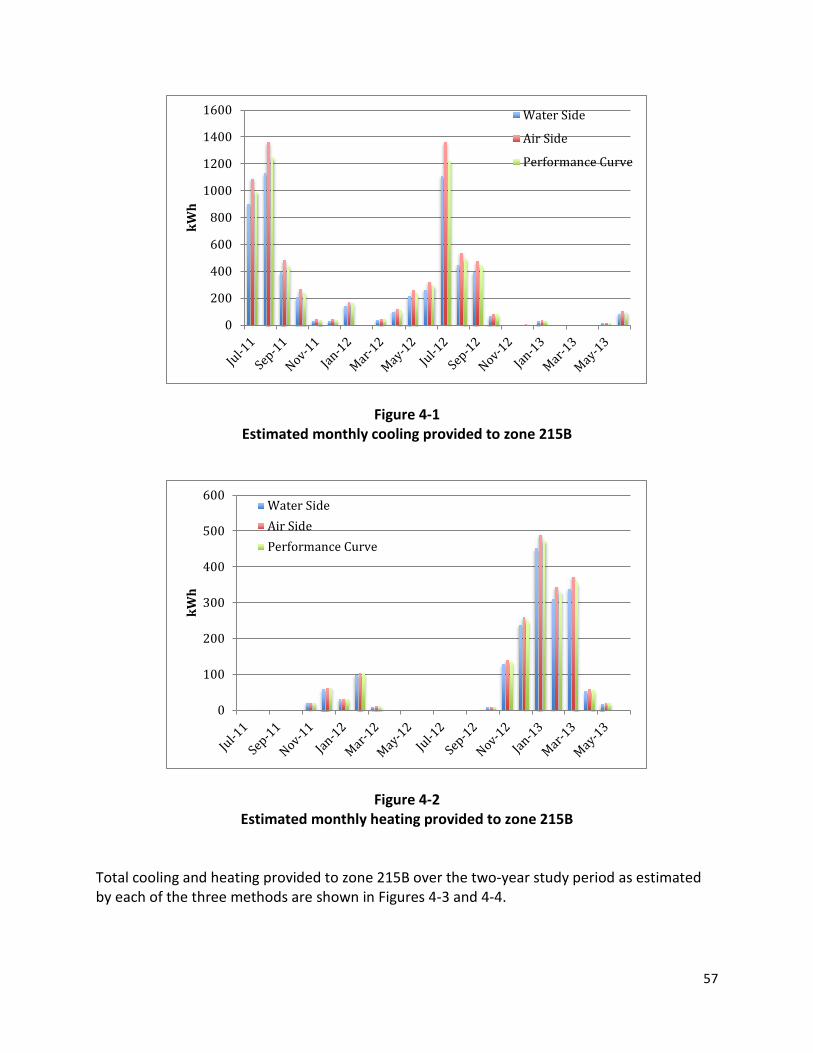
57

Figure 4-1 Estimated monthly cooling provided to zone 215B

Figure 4-2 Estimated monthly heating provided to zone 215B

Total cooling and heating provided to zone 215B over the two-year study period as estimated by each of the three methods are shown in Figures 4-3 and 4-4.

0

200

400

600

800

1000

1200

1400

1600

kWh

Water Side

Air Side

Performance Curve

0

100

200

300

400

500

600

kWh

Water SideAir SidePerformance Curve

58

Figure 4-3 Estimated total two year cooling provided to zone 215B

Figure 4-4 Estimated total two year heating provided to zone 215B

The estimates agree within the uncertainty of the three different methods used. 4.2 Estimates of GSHP system cooling and heating provided

0

1000

2000

3000

4000

5000

6000

7000

8000

9000

Ground Loop Air Side Performance Curve

kWh

0

500

1000

1500

2000

2500

Ground Loop Air Side Performance Curve

kWh

59

All three methods were used to estimate heating and cooling provided by the GSHP system. As noted before, the ground loop estimates only give information about the net cooling or heating load of the system at a given time step. Figures 4-5 through 4-7 compare the estimates of the monthly cooling, heating and net cooling provided by each of the three methods for the GSHP system. Table 4-2 lists the numerical values of cooling and heating provided for each month.

Figure 4-5 Estimated monthly cooling provided for GSHP system

0

2000

4000

6000

8000

10000

12000

14000

16000

18000

20000

kWh

Ground Loop

Air Side Measurements

Performance Curves

60

Figure 4-6 Estimated monthly heating provided for GSHP system

Figure 4-7 Estimated monthly net cooling provided for GSHP system

0

500

1000

1500

2000

2500

3000

3500

4000

4500

kWh

Ground Loop

Air Side Measurements

Performance Curves

-5000

0

5000

10000

15000

20000

kWh

Ground Loop

Air Side Measurements

Performance Curves

61

Table 4-2 Estimated cooling and heating provided by GSHP system

Ground Loop Air Side Performance Curve

Month Cooling Heating Net Cooling

Cooling Heating Net Cooling

Cooling Heating Net Cooling

Jul-11 10898 29 10869 14708 0 14708 14099 0 14099 Aug-11 11882 32 11850 16588 0 16588 15602 0 15602 Sep-11 6052 18 6034 8087 0 8087 7759 0 7759 Oct-11 2924 357 2568 3868 363 3504 3797 384 3413 Nov-11 1714 928 786 2284 987 1295 2223 1084 1139 Dec-11 1176 2698 -1522 1820 2840 -1024 1790 3114 -1325 Jan-12 781 3533 -2752 1397 3754 -2367 1504 4129 -2625 Feb-12 1359 2106 -747 1789 2209 -421 1912 2412 -500 Mar-12 3694 328 3365 4848 343 4505 4773 371 4402 Apr-12 4143 99 4044 5100 106 4993 5248 119 5129

May-12 7202 17 7185 9963 0 9963 9144 0 9144 Jun-12 8202 18 8185 11467 0 11467 10427 0 10427 Jul-12 12413 14 12399 17751 0 17751 16799 0 16799

Aug-12 9167 17 9150 13212 0 13212 12028 0 12028 Sep-12 5951 28 5923 8373 0 8373 7751 0 7751 Oct-12 3622 306 3316 5037 329 4708 4939 350 4588 Nov-12 1031 1705 -673 1587 1967 -382 1771 2123 -352 Dec-12 635 2733 -2098 1203 3235 -2035 1317 3348 -2031 Jan-13 839 2931 -2092 1391 3487 -2101 1651 3613 -1963 Feb-13 615 2968 -2353 851 3394 -2551 1207 3629 -2423 Mar-13 625 3376 -2752 766 3666 -2906 1121 3827 -2706 Apr-13 2182 360 1822 3105 314 2790 3193 321 2872

May-13 3609 209 3400 5208 136 5072 4960 135 4825 Jun-13 6408 33 6375 8772 3 8769 7436 8 7428

62

Total cooling and heating provided by the GSHP system over the two-year study period as estimated by each of the three methods are shown in Figures 4-8 and 4-9.

Figure 4-8 Estimated total two year cooling provided by GSHP system

Figure 4-9 Estimated total two year heating provided by GSHP system

Performance curve and air side estimates were very close to each other, and well within the uncertainty of the estimates; while ground loop estimates were somewhat lower.

0

20

40

60

80

100

120

140

160

180

Ground Loop Air Side Performance Curve

MW

h

0

5

10

15

20

25

30

35

Ground Loop Air Side Performance Curve

MW

h

63

4.3 Estimates of VRF system cooling and heating provided The ground loop and performance curve methods were not applicable to the VRF system, and, as noted in section 3.3, equipment modifications made the data needed to estimate heating and cooling by the air side method unavailable after March 2012. Figures 4-10 through 4-12 show the estimates of heating and cooling provided by the air side method before the equipment was modified.

Figure 4-10 Estimated monthly cooling provided for VRF system

-2000

0

2000

4000

6000

8000

10000

12000

14000

16000

kWh

Air Side Measurements

64

Figure 4-11 Estimated monthly heating provided for VRF system

Figure 4-12 Estimated monthly net cooling provided and model-predicted loads for VRF system

The uncertainty associated with the estimated cooling provided by the VRF system is ±5% and that for the total heating provided is ±4%

0

1000

2000

3000

4000

5000

6000

7000

8000

9000

10000

kWh

Air Side Measurements

-10000

-5000

0

5000

10000

15000

20000

kWh

Air Side Measurements

65

4.4 Estimate of DOAS system cooling provided As noted in section 3.4, measured data is available for the DOAS supply air temperature and humidity, exhaust air temperature and humidity and air flow rates to the first and second floors. These air side measurements are sufficient to estimate the cooling provided using equation 3-9. Figure 4-13 shows the estimated monthly cooling provided by the DOAS system.

Figure 4-13 Estimated monthly cooling provided by DOAS system

For the first three months of the study (July – September, 2011), air side measurements are available for all three HVAC systems during a period when only cooling should have been needed. For this period of time, Figure 4-14 shows the percent of the total building cooling that was provided by each system.

0

2000

4000

6000

8000

10000

12000

kWh

66

Figure 4-14 Contribution of HVAC systems to total building cooling, July – September 2011

4.5 Performance metrics To calculate system heating and cooling COPs, it is necessary to know how much energy was used for each mode of operation but only total system power measurements are available. When all units are running in the same mode (heating only or cooling only), the energy used can be allocated accordingly. When individual heat pump units were running in different modes simultaneously, GSHP system energy use was allocated by the ratio of power used by each unit as estimated by the performance curve method:

(4-1)

where, Esystem,total = total measured system energy use Esystem,cooling = system energy allocated to cooling Esystem,heating = system energy allocated to heating Eunit = individual heat pump energy use (estimated by performance curve) Eunit,cooling = heat pump energy use by unit in cooling mode

41.0%

36.0%

23.0%

GSHP

VRF

DOAS

67

Eunit,heating = heat pump energy use by unit in heating mode Energy use by the VRF system was allocated to heating or cooling based on the nominal capacity of each FCU that was running:

(4-2)

where, Cunit,on = nominal capacity of individual FCU that is operating Cunit,cooling = nominal capacity of FCU in cooling mode Cunit,heating = nominal capacity of FCU in heating mode Since air side measurements for the GSHP system show good agreement with performance curve estimates, take into account simultaneous heating and cooling operation, and could be used to estimate VRF system cooling and heating for part of the study, they were used to calculate the system heating and cooling COP of the GSHP system and of the VRF system for July 2011 through March 2012. Figures 4-15 and 4-16 show the monthly heating and cooling COPs of both systems.

Figure 4-15 Monthly system cooling COPs estimated by air side method

0.0

1.0

2.0

3.0

4.0

5.0

6.0

Cool

ing

COP

GSHP VRF

68

Figure 4-16 Monthly system heating COPs estimated by air side method

Figure 4-15 unexpectedly shows that GSHP system cooling COPs are lower in winter when temperatures are more favorable for cooling. This is because only a few units are running in cooling mode, providing only a small amount of cooling, while there is still a significant amount of system energy use associated with running the blowers in ventilation mode for all the rest of the units. Also, with only a small number of units running, the water loop flow rates are low, and the circulation pump and variable speed drive are less efficient at lower flow rates. Chapter 5 contains a complete analysis of the power use of the GSHP system. Figure 4-15 also shows unusually low cooling COPs for the GSHP system in March, April and May of 2013. During these months, the weather was mild, and the second floor needed little cooling; however, the 2-ton heat pump for zone 202 ran constantly in cooling mode during occupied hours without providing any real cooling due to a malfunctioning reversing valve. Thus, power use for cooling was high due to the constant operation of the heat pump for zone 202, but cooling provided was minimal, resulting in low system cooling COPs for those months. Figure 4-16 shows an increase in heating COPs for the GSHP system in the winter of 2012-2013 when compared with the previous winter. The differential pressure set point on the ground loop was decreased from 20 psi to 8 psi in the spring of 2012, which reduced pumping power and increased system COP. Colder weather creating higher heating demand also contributed to this improved system COP. While this seems counterintuitive, it is the result of higher system utilization which, in turn, means less pumping and fan energy per unit of heating provided and improved system COP. Figures 4-15 and 4-16 do not represent individual unit performance. They represent total system performance including all of the measured energy used by each system. This measured

0.0

1.0

2.0

3.0

4.0

5.0

6.0

Heat

ing

Syst

em C

OP

GSHP VRF

69

energy includes fan power in ventilation mode, standby power consumption, and, for the GSHP system, pumping power.

Figure 4-17 shows the monthly system cooling COPs for the DOAS system as estimated by the air side measurements, which is the only estimation method available for that system. These COPs are estimated from the amount of cooling that was required to cool ambient air to the DOAS supply air temperature using equation 3-9 at each time step where the ambient air temperature is above the DOAS supply air temperature. They are an indication of the efficiency of the DOAS system for cooling the outdoor air to the desired supply temperature. They are not based on the cooling supplied to the building, which would be based on the enthalpy differential between the supply and exhaust air.

Figure 4-17 Monthly DOAS system cooling COP

Like the GSHP system monthly cooling COPs shown in Figure 4-15, the actual cooling provided in winter months is quite low, while the power needed to run the ventilation fans is substantial, causing the DOAS system COPs to be low. For the first three months of the study (July – September 2011), when air side measurements are available for all three systems, and only cooling should have been needed, system cooling COPs can be calculated for each system. For this time period the GSHP system cooling COP was 4.6, the VRF system cooling COP was 3.1 and the DOAS system cooling COP was 2.9.

0

0.5

1

1.5

2

2.5

3

3.5

Cool

ing

COP

70

Chapter 5

GSHP System Energy Analysis

Not all of the energy used by a GSHP system is power input to the individual heat pumps units while the compressors are running. There is a significant energy use by the circulation pumps, the blowers of units that are in ventilation mode, and the unit controls while units are in standby mode overnight and on weekends. The contribution of each of these parts of the system to total energy use was analyzed in an effort to identify ways to improve the GSHP system COP. 5.1 Heat pump energy Performance curve models were used to estimate heat pump power as explained in section 3.2. As noted in section 3.1.2, the measured power use of a 3-ton heat pump during a one-day site visit was 5-8% higher than the performance curve estimate. Total heat pump energy use was calculated as the sum of the energy use of all the units that were running.

(5-1)

where, Esystem,heatpumps = energy used by the heat pumps while running Eunit = individual heat pump energy use (estimated by performance curve) 5.2 Standby energy use Overnight and on weekends the average system power use when all heat pumps and the circulating pump were off, was 384 W or 27W/unit. According to a representative from Climatemaster (Hern, 2014) the normal standby power of the units should be in the 8-10W range for the unit control board and fan ECM. During the site visit the average standby power draw measured for the 3-ton unit in zone 215B was 18 W. Graphs of the raw data from the site visit are included in Appendix C. An explanation for the discrepancy between the expected standby power usage and the measured power use has not been identified. There is also some standby power use for the circulation pump VFDs. Power measurements during the site visit showed a constant power draw of 10 W ± 5 W while the circulation pump was not running. Panel cards for the building show that the power for the BAS control panel is metered with the GSHP system power as well. Since information about BAS control panel power use is not readily available, hourly standby energy use was estimated as being proportional to the number of heat pumps in standby mode:

71

(5-2)

where, Esystem,standby = hourly system standby energy use, W-h onall = number of heat pumps that are on in any mode – ventilation, heat, cool 5.3 Circulation pump energy use The circulation pump is a Bell & Gossett centrifugal pump with 8 ⅞” impeller with a variable frequency drive and identical backup. Maximum pump speed is 1750 RPM. The pump efficiency was modeled with the Brandemuehl approach (Brandemuehl, et al., 1993):

(5-3)

where, η = pump efficiency b0,b1,b2 = correlation coefficients ϕ = dimensionless flow rate Q = volumetric flow rate, m3/sec N = rotational speed, 1/sec D = impeller diameter, m Spump = measured pump speed, % For the Bell & Gossett circulation pump, the model coefficients are:

Table 5-1 Circulation pump model coefficients

b0 0.1303 b1 45.618 b2 -1103.5

A comparison of manufacturer data for pump efficiency and modeled efficiency at 1750 RPM is shown in Figure 5-1.

72

Figure 5-1 Water loop circulation pump curve – 1750 RPM

Based on the piping plans for the building, the pressure drop through the building loop was estimated to be:

(5-4) where, ΔP = pressure drop, Pa Ground loop pressure drop was modeled as 238 feet of 2” SDR-11 HDPE pipe with fittings having a total K value of 6.86 and 870 feet of 1 ¼” SDR-11 HDPE pipe with fitting having a total K value of 3.6 Total pressure drop of the system was modeled as the sum of the pressure drop through the building loop, the pressure drop through the ground loop and the loop differential pressure set point. Theoretical power was calculated as the product of measured loop flow rate and modeled pressure drop. Based on data published by the Advanced Manufacturing Office of the Department of Energy (DOE, 2012), the efficiency of the variable speed drive was modeled as:

(5-5)

where, Load = pump power draw, kW The complete pump power model was developed as an Excel VBA function which implemented equations 5-3, 5-4 and 5-5 along with standard pressure drop calculations. The function

0

0.1

0.2

0.3

0.4

0.5

0.6

0.7

0 50 100 150 200

Pum

p Ef

ficie

ncy

Flow Rate, GPM

Pump curve data points

Pump model

73

required inputs of pump speed, ground loop flow rate and loop differential pressure set point to determine the power used for pumping. During the site visit, the Georgia Power representative also installed power-monitoring equipment on the circuit for the ground loop circulation pumps. Graphs of the raw data from the site visit are included in Appendix C, and a file containing the raw data is included in the electronic archive that accompanies this thesis. Pumping power was measured at ten-minute intervals for 24 hours; however, loop differential pressure was measured at fifteen-minute intervals, and the clocks on the power monitoring equipment were not synchronized with the BAS clock. This made approximately coincident data to compare modeled power with measured power available only at 30-minute intervals. At first the data was collected with the loop differential pressure set at 8 psi. The differential pressure was raised to 15 psi for the last three hours of power monitoring. Figure 5-2 shows the measured pumping power vs. loop flow rate, while Figure 5-3 shows both the measured and modeled power.

Figure 5-2 Measured pumping power vs. loop flow rate

0.000.100.200.300.400.500.600.700.800.901.00

0 5 10 15 20 25 30 35

Mea

sure

d Po

wer

, kW

Loop Flow, GPM

8 psi loop dp

15 psi loop dp

74

Figure 5-3 Measured and model-predicted pumping power

Figure 5-4 shows the comparison of measured and model-predicted pumping power.

Figure 5-4 Pumping power model calibration

Based on the Excel trendline fit in Figure 5-4, a correction factor of 1.4249 was applied to the pump model.

0.00

0.10

0.20

0.30

0.40

0.50

0.60

0.70

0.80

0.90

1.00

12:00 18:00 0:00 6:00 12:00

Pum

ping

Pow

er, k

W

Modeled Measured

y = 1.4249x R² = 0.8052

0.000.100.200.300.400.500.600.700.800.901.00

0.00 0.10 0.20 0.30 0.40 0.50 0.60 0.70

Mea

sure

d Po

wer

, kW

Original Modeled Power, kW

75

5.4 Ventilation blower energy use For time steps when the building was occupied but no heat pump units were running, the modeled circulating pump power was subtracted from the measured system power. The remaining power represented the blower power for all 14 heat pumps running in ventilation mode. The average value of blower power for all 14 heat pumps was 967 W or 69 W/unit. During the site visit, the average measured power draw when the 3-ton unit in zone 215B was operating in ventilation mode was 59 W. Graphs of the raw data from the site visit are included in Appendix C. According to manufacturer documents the blowers operate at 270-700 cfm in ventilation mode. When all 14 units are running in ventilation mode the total air flow is 7590 cfm. This corresponds to an estimated blower power use of 0.13 W/cfm. Published data (Ueno, 2010) reports ECM fan efficiencies of 0.15-0.20 W/cfm for air handlers moving 350-550 cfm. Climatemaster ECM fan performance data (Liu, 2014) indicates that power use should be 0.09-0.28 W/cfm for external static pressures of 0.1-0.7” water gauge. Hourly blower energy use was estimated as being proportional to the number of heat pumps that were running in ventilation mode:

(5-6)

where, Esystem,blower = hourly system blower energy use, W-h onblower = number of heat pumps running in ventilation mode 5.5 Complete energy analysis The total energy use of the GSHP system for the two-year study period was 47.6 MWh. Using the modeling approach described in sections 5.1 through 5.4, the total estimated energy use was 49.5 MWh, which is in error by 4%. Using the modeling approach the contributions of each component of the system to the total power use can be estimated as shown in Figure 5-5.

76

Figure 5-5 GSHP system two-year modeled energy use

Figure 5-5 represents the contribution of each component of the system to the total system power consumption over the two-year study period. Modeled monthly energy use varied seasonally as shown in Figure 5-6.

Figure 5-6 GSHP system monthly modeled energy use

8.1%

11.4%

10.2%

70.4%

Standby Mode

Circulating Pumps

Blowers (ventilationonly)

Heat Pumps

0500

100015002000250030003500400045005000

kWh

Heat Pumps

Blowers

Pumps

Standby

77

Figure 5-7 Contribution of each component to modeled monthly total GSHP system energy use

The percent that each component of the GSHP system contributes to the total energy use is displayed in Figure 5-7. In cooler months the blower, circulation pump and standby energy use accounted for a large part of the total, even more than 50% in November 2011. This supports the assertion, made in section 4.6, that the unexpectedly low system cooling COPs in cold weather can be attributed to the energy used by these components of the system. Figures 5-6 and 5-7 also show that the circulation pumps used noticeably more energy before the loop differential pressure set point was changed from 20 psi to 8 psi in early March of 2012. Figures 5-8 and 5-9 show the contributions of each component to the modeled energy use before and after the differential pressure set point was changed.

0%10%20%30%40%50%60%70%80%90%

100%Standby Pumps Blowers Heat Pumps

78

Figure 5-8 GSHP system modeled energy use with 20 psi loop differential pressure

Figure 5-9 GSHP system modeled energy use with 8 psi loop differential pressure

Since July 1, 2013, the GSHP system has experienced a low temperature alarm on one of the heat pump during periods of cold weather. On December 11, 2013 the loop differential pressure was reset to 12 psi, and on March 20, 2014 it was raised to 15 psi.

7.9%

17.7%

10.0% 64.3%

Loop DP = 20 psi

Standby

Pumps

Blowers

Heat Pumps

8.2%

7.4%

10.2%

74.1%

Loop DP = 8 psi

Standby

Pumps

Blowers

Heat Pumps

79

Chapter 6

Conclusions

Several helpful conclusions can be drawn and lessons learned from the analysis that has been performed. Some conclusions can be drawn from the measured data prior to estimating the heating and cooling provided:

• For the two-year time span of this study, the VRF system used 98% more total energy than the GSHP system, 41% more in the summer cooling season (May - September) and 172% more in the winter and shoulder seasons (October – April).

• The DOAS system used more power than the either the VRF or GSHP system. • Although the renovation added a large conference room to the first floor, the area

served by the VRV-III heat recovery system is only about 11% larger than the area served by the GSHP system. The difference in floor area does not account for the difference in energy use. On a square foot basis the VRF system used 79% more total energy than the GSHP system over the two year study period.

• Due to the thermodynamic advantages of rejecting heat to or extracting heat from the ground rather than the air, the GSHP system has better operational efficiencies, particularly in cold weather and in hot weather.

• The control strategies used with the VRF system that involve tightly controlled single set point temperatures for adjacent zones in an open office environment create artificial heating and cooling needs that are not inherent building loads.

• Higher outdoor air flow rates for the first floor decreased the cooling demands and increased the heating demands for the VRF system. Also, the high DOAS flow rates and tightly controlled zone temperatures led to heating operation in warm weather on the first floor.

• Changing the loop differential pressure set point from 20 psi to 8 psi caused the pumping power to drop from 17% of the total GSHP system power to 7%.

In order to evaluate system performance, the amount of heating and cooling provided must be estimated. Such estimates necessarily involve some approximations, for which the uncertainty has been estimated. Three different approaches were used to estimate the heating and cooling provided to the building. Of these, the air side analysis has acceptable uncertainty (+14/-11% for cooling provided by the GSHP system, ±7% for heating provided by the GSHP system, ±5% for cooling provided by the VRF system and ±4% for heating provided by the VRF system) and can be applied to the GSHP system for the entire two-year period between July 2011 and June 2013. It can be applied to the VRF system only through March 2012 because the control boards in the FCUs were changed out, changing the air flow rates, which were not subsequently measured. Several further conclusions can be reached from these estimates:

• Power measurements and estimates of the heating and cooling provided based on air side measurements show that GSHP system cooling COPs are 4.5-4.8 (SEER 15.3-16.4) in

80

the summer and system heating COPs are 3.0-4.8 in the winter. These system COPs include all energy use by the GSHP system, including pumping, fan power in ventilation mode and standby power consumption of the heat pump control boards, BAS control panel and circulation pump VFDs.

• For July – September, 2011 the GSHP system cooling COP was 4.6+0.6/-0.5, the VRF system cooling COP was 3.1±0.2 and the DOAS system cooling COP was 2.9±0.6 based on air side estimates of cooling provided.

• For July - September, 2011 the GSHP system provided 41% of the total building cooling, the VRF system provided 36% and the DOAS system provided 23%.

• For the winter of 2011-2012, the GSHP system heating COP was 3.3±0.2 and the VRF system heating COP was 2.0±0.1 based on air side estimates of heating provided.

• For the summer of 2012, the VRF COPs could not be determined based on air side measurements, but the GSHP system cooling COP was again 4.6+0.6/-0.5.

81

Chapter 7

Recommendations

This study has shown that there are still areas where energy efficiency and operational improvements could be made at the ASHRAE headquarters building:

• A thermal comfort survey that includes information about the zone each respondent’s office is located in would help to determine whether the different zone temperature control strategies have a measurably different result.

• If occupants of the second floor have an acceptable level of thermal comfort in an environment where zone temperatures are not tightly controlled to a single set point, the zone controls for the zone temperatures on the first floor should be reset so that they are allowed to drift farther from the set point before the FCUs turn on (wider deadband). If improved control strategies could eliminate half of the difference between the amount of energy used by the VRF system and the amount used by the GSHP system, on average, 11.7 MWh/year of energy would be saved. At a conservative estimate of $0.10/ kWh, this would be $1,170 in annual savings.

• Once the VRF fan control issues are resolved, both the GSHP and VRF systems (now 6 years old) should be tested, adjusted and balanced again. VRF system zone air flows could then be used to make a more accurate air side estimate of actual heating and cooling provided by the VRF system.

• A more comprehensive fault detection and diagnostic program to identify potential or existing equipment malfunctions from BAS recorded data should be implemented. The reversing valve in zone 202 began malfunctioning in March, 2013. Zone 202 is the upper level of the front stairwell, and does not have any regular occupants, so the malfunction was not noticed and repaired until December, 2013. This caused the heat pump for zone 202 to run constantly during occupied hours for 8 months, wasting energy. Simple logic to monitor discharge air temperatures when the compressor is running could have identified the malfunction within days if not hours.

This study has also raised many more questions and suggested research in the following directions:

• Raising the DOAS supply air set point would transfer a part of the load associated with cooling and dehumidifying the outdoor air to the more efficient VRF and GSHP systems, but it is not clear how much improvement to overall building energy use could be achieved. Raising the DOAS set point would also eliminate some of the additional heating loads that are created by the DOAS in shoulder seasons. The DOAS set point may need to be changed as a function of ambient air temperature or reset seasonally. As noted by Deng, et al (2014), the engineering community is continuing to learn about DOAS design and operations. Many questions about best practices for DOAS systems remain, and a research project to optimize DOAS operations, taking VRF and GSHP

82

system efficiencies into account, could help to answer some of those questions, as well as saving energy at the building.

• Further study should be done to optimize the ground loop differential pressure set point. Making the ground loop differential pressure set point dependent on outside air temperature would allow it to be raised only when outside air temperatures are low enough to warrant freeze protection. This would save the costs associated with additional pumping energy for much of the year. Another option would be to add small booster pumps for the two heat pumps that are located farthest from the ground loop and keep the ground loop differential pressure at a low (8 psi) set point.

• If the DOAS blowers are adequate to supply fresh air to all zones without the need for additional blowers to boost the air pressure, eliminating ventilation mode for the heat pumps and FCUs should be considered. The energy use of the GSHP system could be reduced by 10% if ventilation mode can be eliminated.

• Power monitoring data points are available for the GSHP in zone 215B, but they do not function properly. Fixing the software that processes the raw data to correctly report power use for that heat pump would open a wide array of opportunities for research on heat pump performance in a commercial installation.

• Once the power monitoring data points for zone 215B are reporting data correctly, temporarily shortening the data logging interval for the data points in that zone to five seconds or less would give a wealth of information about the transient performance of the heat pump at startup and shutdown. An attempt to do this during the site visit showed the potential that is available in this data; however, the power data was only logged at one minute intervals and the clock on the power monitoring equipment was set differently from the BAS clock, making it difficult to match data points and use the power data for a study of startup and shutdown performance.

• As a living lab, there are several more data points that would have made the system performance analyses much more accurate:

o Mixed air temperature for each FCU o Water flow rate to each heat pump o Discharge air flow rates for each FCU and heat pump o Mixed air and discharge air humidity sensors for each FCU and heat pump o Power submeter for GSHP circulation pumps o Outside air temperature at the building that is not influenced by direct sunlight

or nearby equipment In addition, the study has shown some areas that designers should take note of:

• Single set point zone control strategies that allow occupants to adjust the set point do not work well in open office environments.

• Improperly balanced supply air from a DOAS can cause the primary HVAC system to operate as reheat for the DOAS supply air.

83

• Careful choice of the differential pressure set point for a ground loop system can significantly reduce the pumping power required, as well as the size of the circulation pumps.

• The energy efficiency analyses that are performed for the mechanical design of new buildings and renovations take into account fan power and GSHP system pumping power, but the seldom consider the power use associated with keeping equipment in standby mode overnight and on weekends. The energy analysis of the GSHP system for the ASHRAE building shows that this standby energy use can be almost as much as the fan energy use, and even more than the pumping energy use.

84

References ALC Controls. 2008. As built drawings ASHRAE national headquarters. Automated Logic Corporation. December 10, 2008. ASHRAE. 2013. Chapter 18 Nonresidential cooling and heating load calculations. 2013 ASHRAE Handbook – Fundamentals. pp. 18.35-18.38. Atlanta: ASHRAE. Aynur, T.N., Y. Hwang and R. Radermacher. 2008. Experimental evaluation of the ventilation effects on the performance of a VRV system in cooling mode –part I: experimental evaluation. HVAC and R Research 14(4):615-630. B.H.W. Sheet Metal Company. 2008. As built duct layout ASHRAE headquarters addition and renovation. B.H.W. Sheet Metal Company. Jonesboro, GA. May 6, 2008 revision. Bell & Gossett. 2008. ASHRAE Headquarters Renovation Submittal. Bell & Gossett. Morton Grove, IL. February 4, 2008. Brandemuehl, M.J., S. Gabel, and I. Andersen. 1993. A toolkit for secondary HVAC system energy calculations (629-RP). Atlanta: ASHRAE. Choat, E.E. 1999. Resolving duct leakage claims. ASHRAE Journal 41(3):49-53. Climatemaster. 2012. Tranquility 27 (TT) series residential products technical guide. Climatemaster. August 10, 2012 revision. Climatemaster. 2013. Tranquility console (TRC) series submittal data. LC386. Climatemaster. February 8, 2013 revision. Daikin AC, Inc. 2013. VRVIII Brochure. PCVUSE13-05C. Daikin AC (Americas), Inc. Carrollton, TX. Deng, S., J. Lau and J. Jeong. 2014. Do all DOAS configurations provide the same benefits? ASHRAE Journal 57(7):52-57. DOE. 2012. Motor systems tip sheet #11. DOE/GO-102012-3730. Advanced Manufacturing Office, Energy Efficiency & Renewable Energy, U.S. Department of Energy. https://www1.eere.energy.gov/manufacturing/tech_assistance/pdfs/motor_tip_sheet11.pdf. November 2012. Ewbank and Associates. 2008. In-Situ Thermal Conductivity Report, ASHRAE Headquarters, 1791 Tullie Circle, Atlanta, GA. Ewbank and Associates Geothermal Professionals, Fairview, OK. February 8, 2008. Haberl, J.S. and S. Cho. 2004. Literature review of uncertainty of analysis methods. ESL-TR-04/10-03. Energy Systems Laboratory. Texas Engineering Experiment Station, Texas A&M University System. October, 2004. Haberl, J.S., A. Sreshthaputra, D.E. Claridge, and J.K. Kissock. 2003. Inverse model toolkit: application and testing. ASHRAE Transactions 109(2):435-448. Hern, S. 2014. Personal communication with Xiaobing Liu. February 12, 2014. Johnson, Spellman & Associates, Inc. 2007. ASHRAE Headquarters Building Renovation Mechanical Systems Narrative. Johnson, Spellman & Associates, Inc. Norcross, GA. June 26, 2007. Johnson, Spellman & Associates, Inc. 2008. As built construction drawings ASHRAE headquarters addition and renovation. Johnson, Spellman & Associates, Inc. Norcross, GA. April 29, 2008 revision. Kissock, K., J. Haberl, and D. Claridge. 2002. Development of a toolkit for calculating linear, change-point linear and multiple-linear inverse building energy analysis models (RP-1050). ASHRAE Research Project, Final Report. Kwon, L., Y. Hwang, R. Radermacher and B. Kim. 2012. Field performance measurements of a VRF system with sub-cooler in educational offices for the cooling season. Energy and Buildings 49:300-305. Kwon, L., H. Lee, Y. Hwang, R. Radermacher and B. Kim. 2014. Experimental investigation of multifunctional VRF system in heating and shoulder seasons. Applied Thermal Engineering 66(1-2):355-364.

85

Li, H., K. Nagano, Y. Lai, K. Shibata, and H. Fujii. 2013. Evaluating the performance of a large borehole ground source heat pump for greenhouses in northern Japan. Energy 63:387-399. Li, Z., M. Zhao, S. Yu, and H. Li. 2009. A case study of a ground-source heat pump system in an East China office building. Proceedings of 6th International Symposium on Heating, Ventilating and Air Conditioning, ISHVAC 2009, v 3, p 1586-1592. Nanjing China, November 6-9, 2009. Liu, X. 2014. Personal correspondence. February 15, 2014. Liu, X. and T. Hong. 2010. Comparison of energy efficiency between variable refrigerant flow systems and ground source heat pump systems. Energy and Buildings 42(5):584-589. Loose, A., H. Drück, N. Hanke, and F. Thole. 2011. Field test for performance monitoring of combined solar thermal and heat pump systems. 30th ISES Biennial Solar World Congress 2011, SWC 2011, v 5, p 4120-4131. Kassel, Germany, August 28 – September 2, 2011. Puttagunta, S., R.A. Aldrich, D. Owens, and P. Mantha. 2010. Residential ground-source heat pumps: In-field system performance and energy modeling. Transactions – Geothermal Resources Council, v 34(2):863-870. Sacramento, CA, October 24-27, 2010. Richard Wittschiebe Hand. 2007. Ashrae headquarters construction document package. Richard Wittschiebe Hand. Atlanta, GA. June 15, 2007. Spitler, J.D. 2009. Chapter 8 Application of the RTSM – Detailed Example. Load calculation applications manual. pp. 161-167. Atlanta: ASHRAE. TAB Services, Inc. 2008. Test and balance analysis report for ASHRAE headquarters additions and renovations. TAB Services, Inc. Atlanta, GA. August 27, 2008. Taylor, J. R. 1997. An introduction to error analysis: the study of uncertainties in physical measurements. Sausalito, CA: University Science Books. Trane. 2007. Trane custom climate changer air handler submittal. Trane. Lexington, KY. July 20, 2007. Ueno, K. 2010. ECM efficiency better (and worse) than you think. Home Energy May/June 1020:34-38. Vaughn, M.R. 2014. Lessons learned from ASHRAE HW renovation. ASHRAE Journal 56(4):14-30. Wang, S.. 2014. Energy modeling of ground source heat pump vs. variable refrigerant flow systems in representative US climate zones. Energy and Buildings 72:222-228. Zhang, D., X. Zhang and J. Liu. 2011. Experimental study of performance of digital variable multiple air conditioning system under part load conditions. Energy and Buildings 43(6):1175-1178.

Zhao, J., C. Dai, X. Li, Q. Zhu, and L. Li. 2005. A case study of ground source heat pump system in China. Proceedings World Geothermal Congress, 2005, Paper 1473. Antalya, Turkey, April 24-29, 2005.

86

Appendix A

Collected Data Points

Two years worth of data for 559 data points were extracted from the ASHRAE headquarters BAS. The data points for which data were collected are listed in Table A-1.

Table A-1 Collected Data Points

Zone or System Point Describer rm110_vav-110 air flow rm111_vav-111 air flow rm112_vav-112 air flow rm116_vav-116 air flow rm117_vav-117 air flow rm119_vav-119 air flow rm120_vav-120 air flow rm134_vav-134 air flow rm140a_vav-140a air flow rm140b_vav-140b air flow rm145_vav-145 air flow rm204_vav-204 air flow rm206_vav-206 air flow rm215b_vav-215b air flow rm224a_vav-224a air flow rm224c_vav-224c air flow conf_rm219_vav-219 air flow conf_rm227_vav-227 air flow hoteling_rm217_vav-217 air flow hoteling_rm225_vav-225 air flow hoteling_vav-122 air flow library_rm104_vav-104 air flow rm135_vav-135 air flow rm138_vav-138 air flow daikin_fcu-101 run daikin_fcu-101 airflow rate daikin_fcu-101 write setpoint (deg C) daikin_fcu-101 zone CO2 daikin_fcu-101 heating setpoint_OS daikin_fcu-101 ThermoMode daikin_fcu-101 operating mode write

87

daikin_fcu-101 fan status daikin_fcu-101 operating mode daikin_fcu-101 Zone Temp F daikin_fcu-101 Cooling setpoint_OS daikin_fcu-101 Daikin setpoint daikin_fcu-103 run daikin_fcu-103 airflow rate daikin_fcu-103 write setpoint (deg C) daikin_fcu-103 zone CO2 daikin_fcu-103 heating setpoint_OS daikin_fcu-103 ThermoMode daikin_fcu-103 operating mode write daikin_fcu-103 fan status daikin_fcu-103 operating mode daikin_fcu-103 Zone Temp F daikin_fcu-103 Cooling setpoint_OS daikin_fcu-103 Daikin setpoint daikin_fcu-104 run daikin_fcu-104 airflow rate daikin_fcu-104 write setpoint (deg C) daikin_fcu-104 zone CO2 daikin_fcu-104 heating setpoint_OS daikin_fcu-104 ThermoMode daikin_fcu-104 operating mode write daikin_fcu-104 fan status daikin_fcu-104 operating mode daikin_fcu-104 Zone Temp F daikin_fcu-104 Cooling setpoint_OS daikin_fcu-104 Daikin setpoint daikin_fcu-105 run daikin_fcu-105 airflow rate daikin_fcu-105 write setpoint (deg C) daikin_fcu-105 zone CO2 daikin_fcu-105 heating setpoint_OS daikin_fcu-105 ThermoMode daikin_fcu-105 operating mode write daikin_fcu-105 fan status daikin_fcu-105 operating mode daikin_fcu-105 Zone Temp F daikin_fcu-105 Cooling setpoint_OS daikin_fcu-105 Daikin setpoint daikin_fcu-109 run

88

daikin_fcu-109 airflow rate daikin_fcu-109 write setpoint (deg C) daikin_fcu-109 zone CO2 daikin_fcu-109 heating setpoint_OS daikin_fcu-109 ThermoMode daikin_fcu-109 fan status daikin_fcu-109 operating mode daikin_fcu-109 Zone Temp F daikin_fcu-109 Cooling setpoint_OS daikin_fcu-109 Daikin setpoint daikin_fcu-110 run daikin_fcu-110 airflow rate daikin_fcu-110 write setpoint (deg C) daikin_fcu-110 zone CO2 daikin_fcu-110 heating setpoint_OS daikin_fcu-110 ThermoMode daikin_fcu-110 operating mode write daikin_fcu-110 fan status daikin_fcu-110 operating mode daikin_fcu-110 Zone Temp F daikin_fcu-110 Cooling setpoint_OS daikin_fcu-110 Daikin setpoint daikin_fcu-111 run daikin_fcu-111 airflow rate daikin_fcu-111 write setpoint (deg C) daikin_fcu-111 zone CO2 daikin_fcu-111 heating setpoint_OS daikin_fcu-111 ThermoMode daikin_fcu-111 operating mode write daikin_fcu-111 fan status daikin_fcu-111 operating mode daikin_fcu-111 Zone Temp F daikin_fcu-111 Cooling setpoint_OS daikin_fcu-111 Daikin setpoint daikin_fcu-112 run daikin_fcu-112 airflow rate daikin_fcu-112 Daikin setpoint daikin_fcu-112 write setpoint (deg C) daikin_fcu-112 zone CO2 daikin_fcu-112 heating setpoint_OS daikin_fcu-112 ThermoMode daikin_fcu-112 operating mode write

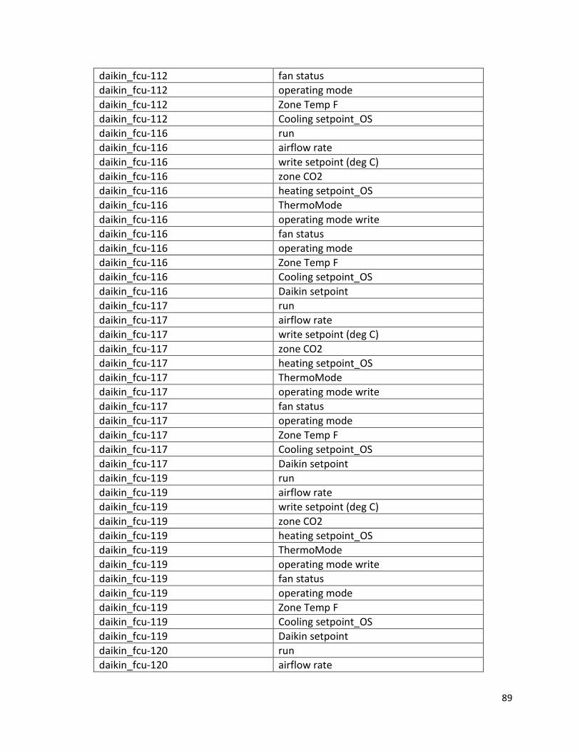
89

daikin_fcu-112 fan status daikin_fcu-112 operating mode daikin_fcu-112 Zone Temp F daikin_fcu-112 Cooling setpoint_OS daikin_fcu-116 run daikin_fcu-116 airflow rate daikin_fcu-116 write setpoint (deg C) daikin_fcu-116 zone CO2 daikin_fcu-116 heating setpoint_OS daikin_fcu-116 ThermoMode daikin_fcu-116 operating mode write daikin_fcu-116 fan status daikin_fcu-116 operating mode daikin_fcu-116 Zone Temp F daikin_fcu-116 Cooling setpoint_OS daikin_fcu-116 Daikin setpoint daikin_fcu-117 run daikin_fcu-117 airflow rate daikin_fcu-117 write setpoint (deg C) daikin_fcu-117 zone CO2 daikin_fcu-117 heating setpoint_OS daikin_fcu-117 ThermoMode daikin_fcu-117 operating mode write daikin_fcu-117 fan status daikin_fcu-117 operating mode daikin_fcu-117 Zone Temp F daikin_fcu-117 Cooling setpoint_OS daikin_fcu-117 Daikin setpoint daikin_fcu-119 run daikin_fcu-119 airflow rate daikin_fcu-119 write setpoint (deg C) daikin_fcu-119 zone CO2 daikin_fcu-119 heating setpoint_OS daikin_fcu-119 ThermoMode daikin_fcu-119 operating mode write daikin_fcu-119 fan status daikin_fcu-119 operating mode daikin_fcu-119 Zone Temp F daikin_fcu-119 Cooling setpoint_OS daikin_fcu-119 Daikin setpoint daikin_fcu-120 run daikin_fcu-120 airflow rate

90

daikin_fcu-120 write setpoint (deg C) daikin_fcu-120 zone CO2 daikin_fcu-120 heating setpoint_OS daikin_fcu-120 ThermoMode daikin_fcu-120 operating mode write daikin_fcu-120 fan status daikin_fcu-120 operating mode daikin_fcu-120 Zone Temp F daikin_fcu-120 Cooling setpoint_OS daikin_fcu-120 Daikin setpoint daikin_fcu-130a airflow rate daikin_fcu-130a write setpoint (deg C) daikin_fcu-130a zone CO2 daikin_fcu-130a ThermoMode daikin_fcu-130a fan status daikin_fcu-130a operating mode daikin_fcu-130a Zone Temp F daikin_fcu-130a Cooling setpoint_OS daikin_fcu-130a Daikin setpoint daikin_fcu-130b airflow rate daikin_fcu-130b write setpoint (deg C) daikin_fcu-130b zone CO2 daikin_fcu-130b ThermoMode daikin_fcu-130b fan status daikin_fcu-130b operating mode daikin_fcu-130b Zone Temp F daikin_fcu-130b Cooling setpoint_OS daikin_fcu-130b Daikin setpoint daikin_fcu-134a run daikin_fcu-134a airflow rate daikin_fcu-134a write setpoint (deg C) daikin_fcu-134a zone CO2 daikin_fcu-134a heating setpoint_OS daikin_fcu-134a ThermoMode daikin_fcu-134a operating mode write daikin_fcu-134a fan status daikin_fcu-134a operating mode daikin_fcu-134a Zone Temp F daikin_fcu-134a Cooling setpoint_OS daikin_fcu-134a Daikin setpoint daikin_fcu-134b run daikin_fcu-134b airflow rate

91

daikin_fcu-134b write setpoint (deg C) daikin_fcu-134b zone CO2 daikin_fcu-134b heating setpoint_OS daikin_fcu-134b ThermoMode daikin_fcu-134b operating mode write daikin_fcu-134b fan status daikin_fcu-134b operating mode daikin_fcu-134b Zone Temp F daikin_fcu-134b Cooling setpoint_OS daikin_fcu-134b Daikin setpoint daikin_fcu-134c run daikin_fcu-134c airflow rate daikin_fcu-134c write setpoint (deg C) daikin_fcu-134c zone CO2 daikin_fcu-134c heating setpoint_OS daikin_fcu-134c ThermoMode daikin_fcu-134c operating mode write daikin_fcu-134c fan status daikin_fcu-134c operating mode daikin_fcu-134c Zone Temp F daikin_fcu-134c Cooling setpoint_OS daikin_fcu-134c Daikin setpoint daikin_fcu-134d run daikin_fcu-134d airflow rate daikin_fcu-134d write setpoint (deg C) daikin_fcu-134d zone CO2 daikin_fcu-134d heating setpoint_OS daikin_fcu-134d ThermoMode daikin_fcu-134d operating mode write daikin_fcu-134d fan status daikin_fcu-134d operating mode daikin_fcu-134d Zone Temp F daikin_fcu-134d Cooling setpoint_OS daikin_fcu-134d Daikin setpoint daikin_fcu-139 run daikin_fcu-139 airflow rate daikin_fcu-139 write setpoint (deg C) daikin_fcu-139 zone CO2 daikin_fcu-139 heating setpoint_OS daikin_fcu-139 ThermoMode daikin_fcu-139 operating mode write daikin_fcu-139 fan status

92

daikin_fcu-139 operating mode daikin_fcu-139 Zone Temp F daikin_fcu-139 Cooling setpoint_OS daikin_fcu-139 Daikin setpoint daikin_fcu-140a run daikin_fcu-140a airflow rate daikin_fcu-140a write setpoint (deg C) daikin_fcu-140a zone CO2 daikin_fcu-140a heating setpoint_OS daikin_fcu-140a ThermoMode daikin_fcu-140a operating mode write daikin_fcu-140a fan status daikin_fcu-140a operating mode daikin_fcu-140a Zone Temp F daikin_fcu-140a Cooling setpoint_OS daikin_fcu-140a Daikin setpoint daikin_fcu-140b run daikin_fcu-140b airflow rate daikin_fcu-140b write setpoint (deg C) daikin_fcu-140b zone CO2 daikin_fcu-140b heating setpoint_OS daikin_fcu-140b ThermoMode daikin_fcu-140b operating mode write daikin_fcu-140b fan status daikin_fcu-140b operating mode daikin_fcu-140b Zone Temp F daikin_fcu-140b Cooling setpoint_OS daikin_fcu-140b Daikin setpoint daikin_fcu-140c run daikin_fcu-140c airflow rate daikin_fcu-140c write setpoint (deg C) daikin_fcu-140c zone CO2 daikin_fcu-140c heating setpoint_OS daikin_fcu-140c ThermoMode daikin_fcu-140c operating mode write daikin_fcu-140c fan status daikin_fcu-140c operating mode daikin_fcu-140c Zone Temp F daikin_fcu-140c Cooling setpoint_OS daikin_fcu-140c Daikin setpoint daikin_fcu-145 run daikin_fcu-145 airflow rate

93

daikin_fcu-145 write setpoint (deg C) daikin_fcu-145 zone CO2 daikin_fcu-145 heating setpoint_OS daikin_fcu-145 ThermoMode daikin_fcu-145 operating mode write daikin_fcu-145 fan status daikin_fcu-145 operating mode daikin_fcu-145 Zone Temp F daikin_fcu-145 Cooling setpoint_OS daikin_fcu-145 Daikin setpoint daikin_fcu-146 run daikin_fcu-146 airflow rate daikin_fcu-146 write setpoint (deg C) daikin_fcu-146 zone CO2 daikin_fcu-146 heating setpoint_OS daikin_fcu-146 ThermoMode daikin_fcu-146 operating mode write daikin_fcu-146 fan status daikin_fcu-146 operating mode daikin_fcu-146 Zone Temp F daikin_fcu-146 Cooling setpoint_OS daikin_fcu-146 Daikin setpoint daikin_fcu-147 run daikin_fcu-147 airflow rate daikin_fcu-147 write setpoint (deg C) daikin_fcu-147 zone CO2 daikin_fcu-147 heating setpoint_OS daikin_fcu-147 ThermoMode daikin_fcu-147 fan status daikin_fcu-147 operating mode daikin_fcu-147 Zone Temp F daikin_fcu-147 Cooling setpoint_OS daikin_fcu-147 Daikin setpoint doas_1st_floor_airflow Flr1 SA Flow doas_2nd_floor_airflow Flr2 SA Flow doas_unit_pwr kw_tn doas1 CDQ2 Lvg RH doas1 CDQ2 Lvg Temp doas1 RA Dewpoint doas1 RA RH doas1 RA Temp fcu-101_zone_data Space Humidity

94

fcu-101_zone_data DATempA fcu-101_zone_data DATempB fcu-103_zone_data Space Humidity fcu-103_zone_data DATempA fcu-103_zone_data DATempB fcu-104_zone_data Space Humidity fcu-104_zone_data DATempA fcu-104_zone_data DATempB fcu-105_zone_data Space Humidity fcu-105_zone_data DATempA fcu-105_zone_data DATempB fcu-109_zone_data Space Humidity fcu-109_zone_data DATempA fcu-109_zone_data DATempB fcu-110111_zone_data Space Humidity fcu-110111_zone_data DATempA fcu-110111_zone_data DATempB fcu-112_zone_data Space Humidity fcu-112_zone_data DATempA fcu-112_zone_data DATempB fcu-116117_zone_data Space Humidity fcu-116117_zone_data DATempA fcu-116117_zone_data DATempB fcu-119120_zone_data Space Humidity fcu-119120_zone_data DATempA fcu-119120_zone_data DATempB fcu-130a_zone_data Space Humidity fcu-130a_zone_data DATempA fcu-130a_zone_data DATempB fcu-130b_zone_data Space Humidity fcu-130b_zone_data DATempA fcu-130b_zone_data DATempB fcu-134a_zone_data Space Humidity fcu-134a_zone_data DATempA fcu-134a_zone_data DATempB fcu-134b_zone_data Space Humidity fcu-134b_zone_data DATempA fcu-134b_zone_data DATempB fcu-134c_zone_data Space Humidity fcu-134c_zone_data DATempA fcu-134c_zone_data DATempB fcu-134d_zone_data Space Humidity

95

fcu-134d_zone_data DATempA fcu-134d_zone_data DATempB fcu-139_zone_data Space Humidity fcu-139_zone_data DATempA fcu-139_zone_data DATempB fcu-140a_zone_data Space Humidity fcu-140a_zone_data DATempA fcu-140a_zone_data DATempB fcu-140b_zone_data Space Humidity fcu-140b_zone_data DATempA fcu-140b_zone_data DATempB fcu-140c_zone_data Space Humidity fcu-140c_zone_data DATempA fcu-140c_zone_data DATempB fcu-145_zone_data Space Humidity fcu-145_zone_data DATempA fcu-145_zone_data DATempB fcu-146_zone_data Space Humidity fcu-146_zone_data DATempA fcu-146_zone_data DATempB fcu-147_zone_data Space Humidity fcu-147_zone_data DATempA fcu-147_zone_data DATempB ground_loop_water_system GLWS Loop Water Flow ground_loop_water_system Loop Water Pump 1 VFD Speed ground_loop_water_system Loop Water Pump 2 VFD Speed ground_loop_water_system LWDP Average ground_loop_water_system Loop Return Temp ground_loop_water_system Loop Supply Temp gt07-141_gshp Comp 1 Start/Stop gt07-141_gshp Discharge Air Temperature gt07-141_gshp Return Air/Zone Temp gt07-141_gshp Reversing Valve (off - heat) gt07-141_gshp Heating Setpoint gt07-141_gshp Cooling Setpoint gt07-232_gshp Comp 1 Start/Stop gt07-232_gshp Comp 2 Start/Stop gt07-232_gshp Discharge Air Temperature gt07-232_gshp Return Air/Zone Temp gt07-232_gshp Reversing Valve (off - heat) gt07-232_gshp Heating Setpoint gt07-232_gshp Cooling Setpoint

96

gt15-207_gshp Comp 1 Start/Stop gt15-207_gshp Comp 2 Start/Stop gt15-207_gshp Discharge Air Temperature gt15-207_gshp Mixed Air Temperature gt15-207_gshp Return Air/Zone Temp gt15-207_gshp Reversing Valve (off - heat) gt15-207_gshp Zone Temperature gt15-207_gshp Heating Setpoint gt15-207_gshp Space Humidity gt18-204_gshp Comp 1 Start/Stop gt18-204_gshp Comp 2 Start/Stop gt18-204_gshp Discharge Air Temperature gt18-204_gshp Mixed Air Temperature gt18-204_gshp Return Air/Zone Temp gt18-204_gshp Reversing Valve (off - heat) gt18-204_gshp Zone Temperature gt18-204_gshp Heating Setpoint gt18-204_gshp Space Humidity gt26-202_gshp Comp 1 Start/Stop gt26-202_gshp Comp 2 Start/Stop gt26-202_gshp Discharge Air Temperature gt26-202_gshp Mixed Air Temperature gt26-202_gshp Return Air/Zone Temp gt26-202_gshp Reversing Valve (off - heat) gt26-202_gshp Zone Temperature gt26-202_gshp Heating Setpoint gt26-202_gshp Space Humidity gt26-209_gshp Comp 1 Start/Stop gt26-209_gshp Comp 2 Start/Stop gt26-209_gshp Discharge Air Temperature gt26-209_gshp Mixed Air Temperature gt26-209_gshp Return Air/Zone Temp gt26-209_gshp Reversing Valve (off - heat) gt26-209_gshp Zone Temperature gt26-209_gshp Heating Setpoint gt26-209_gshp Space Humidity gt26-224c_gshp Comp 1 Start/Stop gt26-224c_gshp Comp 2 Start/Stop gt26-224c_gshp Discharge Air Temperature gt26-224c_gshp Mixed Air Temperature gt26-224c_gshp Return Air/Zone Temp gt26-224c_gshp Reversing Valve (off - heat)

97

gt26-224c_gshp Zone Temperature gt26-224c_gshp Heating Setpoint gt26-224c_gshp Cooling Setpoint gt26-224c_gshp Space Humidity gt26-224d_gshp Comp 1 Start/Stop gt26-224d_gshp Comp 2 Start/Stop gt26-224d_gshp Discharge Air Temperature gt26-224d_gshp Mixed Air Temperature gt26-224d_gshp Return Air/Zone Temp gt26-224d_gshp Reversing Valve (off - heat) gt26-224d_gshp Zone Temperature gt26-224d_gshp Heating Setpoint gt26-224d_gshp Cooling Setpoint gt26-224d_gshp Space Humidity gt38-206_gshp Comp 1 Start/Stop gt38-206_gshp Comp 2 Start/Stop gt38-206_gshp Discharge Air Temperature gt38-206_gshp Mixed Air Temperature gt38-206_gshp Return Air/Zone Temp gt38-206_gshp Reversing Valve (off - heat) gt38-206_gshp Zone Temperature gt38-206_gshp Heating Setpoint gt38-206_gshp Space Humidity gt38-215a_gshp Comp 1 Start/Stop gt38-215a_gshp Comp 2 Start/Stop gt38-215a_gshp Discharge Air Temperature gt38-215a_gshp Mixed Air Temperature gt38-215a_gshp Return Air/Zone Temp gt38-215a_gshp Reversing Valve (off - heat) gt38-215a_gshp Zone Temperature gt38-215a_gshp Heating Setpoint gt38-215a_gshp Cooling Setpoint gt38-215a_gshp Space Humidity gt38-215b Comp 1 Start/Stop gt38-215b Comp 2 Start/Stop gt38-215b Discharge Air Temperature gt38-215b Gnd Loop Flow gt38-215b GLWS(upply) Temp gt38-215b DA flow gt38-215b DA Humidity gt38-215b MA Humidity gt38-215b GLWR(eturn) Temp

98

gt38-215b Mixed Air Temperature gt38-215b Return Air/Zone Temp gt38-215b Reversing Valve (off - heat) gt38-215b Heating Setpoint gt38-215b Cooling Setpoint gt38-215b Space Humidity gt38-215c_gshp Comp 1 Start/Stop gt38-215c_gshp Comp 2 Start/Stop gt38-215c_gshp Discharge Air Temperature gt38-215c_gshp Mixed Air Temperature gt38-215c_gshp Return Air/Zone Temp gt38-215c_gshp Reversing Valve (off - heat) gt38-215c_gshp Zone Temperature gt38-215c_gshp Heating Setpoint gt38-215c_gshp Cooling Setpoint gt38-215c_gshp Space Humidity gt38-224a_gshp Comp 1 Start/Stop gt38-224a_gshp Comp 2 Start/Stop gt38-224a_gshp Discharge Air Temperature gt38-224a_gshp Mixed Air Temperature gt38-224a_gshp Return Air/Zone Temp gt38-224a_gshp Reversing Valve (off - heat) gt38-224a_gshp Zone Temperature gt38-224a_gshp Heating Setpoint gt38-224a_gshp Cooling Setpoint gt38-224a_gshp Space Humidity gt38-224b Comp 1 Start/Stop gt38-224b Comp 2 Start/Stop gt38-224b Discharge Air Temperature gt38-224b Mixed Air Temperature gt38-224b Return Air/Zone Temp gt38-224b Reversing Valve (off - heat) gt38-224b Zone Temperature gt38-224b Heating Setpoint gt38-224b Cooling Setpoint gt38-224b Space Humidity rm_104_aircuity CO2 rm_110_aircuity CO2 rm_111_aircuity CO2 rm_112_aircuity CO2 rm_116_aircuity CO2 rm_117_aircuity CO2

99

rm_119_aircuity CO2 rm_120_aircuity CO2 rm_123_aircuity CO2 rm_130_aircuity CO2 rm_134_aircuity CO2 rm_135_aircuity CO2 rm_138_aircuity CO2 rm_140_aircuity CO2 rm_145_aircuity CO2 rm_206_aircuity CO2 rm_215b_aircuity CO2 rm_217_aircuity CO2 rm_219_aircuity CO2 rm_220_aircuity CO2 rm_224a_aircuity CO2 rm_224c_aircuity CO2 rm_225_aircuity CO2 rm_227_aircuity CO2 first_flr_lighting_system_pwr kw_tn first_flr_plug_loads_pwr kw_tn second_floor_lighting_system_pwr kw_tn second_flr_plug_loads_pwr kw_tn vrv_system_pwr kw_tn heat_pump_system_pwr kw_tn

100

Appendix B

Heat pump performance curve model coefficients

Three different models of heat pumps were used in the ASHRAE headquarters building renovation, TRC09, TTH026 and TTH038. Performance data for these models was provided by Climatemaster (Climatemaster, 2012, Climatemaster, 2013). The performance curves for the TTH038 heat pumps were modeled with generalized least squares curve fits of the form:

(B-1)

Since none of the TRC09 or TTH026 heat pumps had air flow instrumentation, and the building TAB report showed that they all had air flow rates within 5% of design flow rates, the CFM term was dropped, and they were modeled with equations of the form:

(B-2)

where, TC = total capacity, Mbtuh PI = power input, kW EFT = entering fluid temperature, °F GPM = water flow rate, gpm CFM = air flow rate, cfm C1-C7 = correlation coefficients Table B-1 gives the values of the correlation coefficients and the coefficient of variation for each model and operating mode.

101

Table B-1

Correlation coefficients for heat pump performance curve models

Model Load Mode Value C1 C2 C3 C4 C5 C6 C7 cv TRC09 Full Cool TC 7.27 0.0826 0.0450 -1.00e-3 -0.242 0.0147 0.00633 TRC09 Full Cool PI 0.503 -2.39e-4 -0.102 5.42e-5 0.0333 -8.30e-4 0.00492 TRC09 Full Heat TC 1.88 0.128 1.51 -2.63e-4 -0.311 1.67e-3 0.00525 TRC09 Full Heat PI 0.623 1.11e-3 0.0280 3.89e-6 -0.0103 2.74e-4 0.00228

TTH026 Part Cool TC 21.7 0.0423 0.335 -9.86e-4 -0.0230 1.05e-3 0.02142 TTH026 Part Cool PI 0.599 9.11e-4 -0.0327 9.21e-5 2.70e-3 -2.54e-4 0.00733 TTH026 Part Heat TC 4.19 0.271 0.651 -5.81e-4 -0.0511 3.06e-3 0.00301 TTH026 Part Heat PI 0.919 5.97e-3 -4.08e-3 -3.01e-5 1.82e-4 8.10e-5 0.00518 TTH026 Full Cool TC 30.8 -0.0247 0.521 -8.19e-4 -0.0364 2.17e-3 0.01069 TTH026 Full Cool PI 1.083 2.72e-3 -0.0672 1.02e-4 5.00e-3 -3.30e-4 0.00413 TTH026 Full Heat TC 2.92 0.431 1.05 -1.28e-3 -0.0671 2.33e-3 0.00301 TTH026 Full Heat PI 1.14 7.95e-3 0.0234 -5.77e-6 -1.52e-3 9.70e-5 0.00176 TTH038 Part Cool TC 27.2 0.0162 0.589 2.77e-3 -9.87e-4 -0.0386 1.58e-3 0.02147 TTH038 Part Cool PI 0.784 3.23e-3 -0.0964 1.47e-4 1.21e-4 7.10e-3 -3.43e-4 0.00685 TTH038 Part Heat TC 7.41 0.193 0.907 2.40e-3 6.57e-4 -0.0741 7.97e-3 0.00246 TTH038 Part Heat PI 1.86 8.63e-4 4.04e-3 -3.49e-4 7.41e-6 -2.97e-4 3.75e-5 0.00227 TTH038 Full Cool TC 37.3 -0.0599 0.787 5.12e-3 -8.86e-4 -0.0513 3.44e-3 0.00815 TTH038 Full Cool PI 1.07 4.46e-3 -0.114 6.01e-4 1.48e-4 7.60e-3 -5.54e-4 0.01078 TTH038 Full Heat TC 7.93 0.282 1.30 4.80e-3 7.20e-4 -0.0901 0.0113 0.00283 TTH038 Full Heat PI 2.84 5.3e0-5 0.0282 -6.64e-4 7.33e-5 -2.59e-4 4.74e-4 0.00265

108

Entering air temperature (EAT) correction factors were modeled with Excel trendlines of the form:

(B-3)

where, CF = correction factor C1-C3 = correlation coefficients EAT = entering air wet bulb temperature for cooling and dry bulb temperature for heating, °F Table B-2 lists the resulting EAT correction factor equations for each model, operating mode and value.

Table B-2 Entering air temperature correction factor equation coefficients

Model Load Mode Value C1 C2 C3

TRC09 Full Cool TC 2.40e-4 -0.0199 1.26 TRC09 Full Cool PI 4.35e-5 -5.91e-3 1.20 TRC09 Full Heat TC 0 -3.83e-3 1.27 TRC09 Full Heat PI 0 9.06e-3 0.366

TTH026 or TTH038 Part Cool TC 2.48e-4 -0.0221 1.37 TTH026 or TTH038 Part Cool PI 5.70e-6 2.16e-4 0.960 TTH026 or TTH038 Part Heat TC -1.25e-5 -1.44e-3 1.16 TTH026 or TTH038 Part Heat PI 7.72e-5 4.66e-4 0.588 TTH026 or TTH038 Full Cool TC 2.34e-4 -0.0186 1.19 TTH026 or TTH038 Full Cool PI 5.52e-5 -3.72e-3 1.00 TTH026 or TTH038 Full Heat TC -1.25e-5 -3.42e-4 1.08 TTH026 or TTH038 Full Heat PI 5.10e-5 1.77e-3 0.626

109

Appendix C

Power monitoring data

During a site visit to the ASHRAE headquarters building on May 5-6, 2014, a representative from Georgia Power temporarily installed power-monitoring equipment on the circuit that provides power to the heat pump for zone 215B, which is a 3-ton heat pump and on the circuit that provides power to the ground loop circulation pumps. Graphs of the raw data from those measurements are included below. Files containing the raw data are included in the electronic archive that accompanies this thesis. Figures C-1 through C-3 contain power data for heat pump 215B. Figure C-4 shows power data for the ground loop circulation pumps.

Figure C-1 Measured power for heat pump 215B

110

Figure C-2 Measured power data for heat pump 215B in ventilation mode on May 5, 2014

Figure C-3 Overnight measured power data for heat pump 215B

Figure C-4 Measured power data for ground loop circulation pump

A plot of measured pumping power vs. ground loop flow rate is in Figure 5-2.

GEO – The Geothermal Exchange Organization 312 South 4th Street Springfield, IL 62701 Phone (888) 255-4436 Email GEO@geoexchange.org Website www.geoexchange.org