Embed Size (px)
Citation preview
Institutionen för systemteknikDepartment of Electrical Engineering
Examensarbete
Performance estimation of a ducted fan UAV
Examensarbete utfört i Reglerteknikvid Tekniska högskolan i Linköping
av
Mattias ErikssonBjörn Wedell
LITH-ISY-EX--06/3795--SE
Linköping 2006
Department of Electrical Engineering Linköpings tekniska högskolaLinköpings universitet Linköpings universitetSE-581 83 Linköping, Sweden 581 83 Linköping

Performance estimation of a ducted fan UAV
Examensarbete utfört i Reglerteknikvid Tekniska högskolan i Linköping
av
Mattias ErikssonBjörn Wedell
LITH-ISY-EX--06/3795--SE
Handledare: Johan SjöbergISY, Linköpings tekniska högskola
Jan-Erik StrömbergDST Control AB
Examinator: Anders HanssonISY, Linköpings tekniska högskola
Linköping, 29 March, 2006

Avdelning, InstitutionDivision, Department
Division of Automatic ControlDepartment of Electrical EngineeringLinköpings universitetS-581 83 Linköping, Sweden
DatumDate
2006-03-29
SpråkLanguage
Svenska/Swedish Engelska/English
RapporttypReport category
Licentiatavhandling Examensarbete C-uppsats D-uppsats Övrig rapport
URL för elektronisk versionurn.kb.se/resolve?urn=urn:nbn:se:liu:diva-6216
ISBN—
ISRNLITH-ISY-EX--06/3795--SE
Serietitel och serienummerTitle of series, numbering
ISSN—
TitelTitle
Prestandaberäkning för en tunnlad fläkt-UAVPerformance estimation of a ducted fan UAV
FörfattareAuthor
Mattias Eriksson, Björn Wedell
SammanfattningAbstract
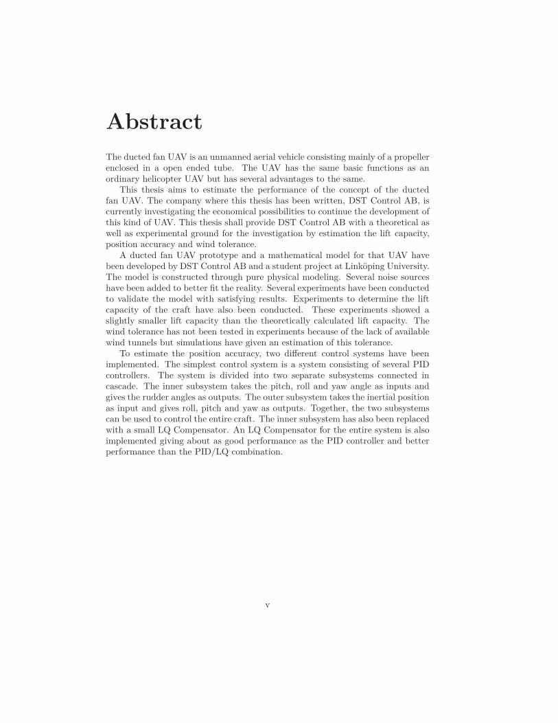
The ducted fan UAV is an unmanned aerial vehicle consisting mainly of a propellerenclosed in a open ended tube. The UAV has the same basic functions as anordinary helicopter UAV but has several advantages to the same.
This thesis aims to estimate the performance of the concept of the ductedfan UAV. The company where this thesis has been written, DST Control AB, iscurrently investigating the economical possibilities to continue the development ofthis kind of UAV. This thesis shall provide DST Control AB with a theoretical aswell as experimental ground for the investigation by estimation the lift capacity,position accuracy and wind tolerance.
A ducted fan UAV prototype and a mathematical model for that UAV havebeen developed by DST Control AB and a student project at Linköping Univer-sity. The model is constructed through pure physical modeling. Several noisesources have been added to better fit the reality. Several experiments have beenconducted to validate the model with satisfying results. Experiments to determinethe lift capacity of the craft have also been conducted. These experiments showeda slightly smaller lift capacity than the theoretically calculated lift capacity. Thewind tolerance has not been tested in experiments because of the lack of availablewind tunnels but simulations have given an estimation of this tolerance.
To estimate the position accuracy, two different control systems have beenimplemented. The simplest control system is a system consisting of several PIDcontrollers. The system is divided into two separate subsystems connected incascade. The inner subsystem takes the pitch, roll and yaw angle as inputs andgives the rudder angles as outputs. The outer subsystem takes the inertial positionas input and gives roll, pitch and yaw as outputs. Together, the two subsystemscan be used to control the entire craft. The inner subsystem has also been replacedwith a small LQ Compensator. An LQ Compensator for the entire system is alsoimplemented giving about as good performance as the PID controller and betterperformance than the PID/LQ combination.
NyckelordKeywords ducted fan, UAV, LQ, PID

AbstractThe ducted fan UAV is an unmanned aerial vehicle consisting mainly of a propellerenclosed in a open ended tube. The UAV has the same basic functions as anordinary helicopter UAV but has several advantages to the same.
This thesis aims to estimate the performance of the concept of the ductedfan UAV. The company where this thesis has been written, DST Control AB, iscurrently investigating the economical possibilities to continue the development ofthis kind of UAV. This thesis shall provide DST Control AB with a theoretical aswell as experimental ground for the investigation by estimation the lift capacity,position accuracy and wind tolerance.
A ducted fan UAV prototype and a mathematical model for that UAV havebeen developed by DST Control AB and a student project at Linköping University.The model is constructed through pure physical modeling. Several noise sourceshave been added to better fit the reality. Several experiments have been conductedto validate the model with satisfying results. Experiments to determine the liftcapacity of the craft have also been conducted. These experiments showed aslightly smaller lift capacity than the theoretically calculated lift capacity. Thewind tolerance has not been tested in experiments because of the lack of availablewind tunnels but simulations have given an estimation of this tolerance.
To estimate the position accuracy, two different control systems have beenimplemented. The simplest control system is a system consisting of several PIDcontrollers. The system is divided into two separate subsystems connected incascade. The inner subsystem takes the pitch, roll and yaw angle as inputs andgives the rudder angles as outputs. The outer subsystem takes the inertial positionas input and gives roll, pitch and yaw as outputs. Together, the two subsystemscan be used to control the entire craft. The inner subsystem has also been replacedwith a small LQ Compensator. An LQ Compensator for the entire system is alsoimplemented giving about as good performance as the PID controller and betterperformance than the PID/LQ combination.
v

Acknowledgements
We would like to thank our supervisors Johan Sjöberg at Linköping Instituteof Technology and Jan-Erik Strömberg at DST Control AB for their help withquestions of all kinds. We would also like to thank our examiner Anders Hanssonfor his initial help and our master thesis colleague Martin Alkeryd for his helpwith the practical aspects of the project.
Furthermore we would like to thank all the helpful people at DST Control ABfor their patience and understanding of our work, the people at CybAero AB forthe help we received when we constructed the test rig and the people at ImpactCoating AB for their patience with our loud craft.
Finally, we would like to thank the students who carried out the initial projectat DST Control AB for their initial help explaining the software and hardware.
vii

Contents
1 Introduction 51.1 Purpose . . . . . . . . . . . . . . . . . . . . . . . . . . . . . . . . . 51.2 Goals . . . . . . . . . . . . . . . . . . . . . . . . . . . . . . . . . . 51.3 Extent and Limitations . . . . . . . . . . . . . . . . . . . . . . . . 51.4 Background . . . . . . . . . . . . . . . . . . . . . . . . . . . . . . . 61.5 Available Hardware and Software . . . . . . . . . . . . . . . . . . . 61.6 Structure of this Document . . . . . . . . . . . . . . . . . . . . . . 6
2 Theory 92.1 Unmanned Aerial Vehicle . . . . . . . . . . . . . . . . . . . . . . . 92.2 Ducted Fan . . . . . . . . . . . . . . . . . . . . . . . . . . . . . . . 92.3 Vectored Thrust . . . . . . . . . . . . . . . . . . . . . . . . . . . . 102.4 Definitions . . . . . . . . . . . . . . . . . . . . . . . . . . . . . . . . 10
3 Rig 133.1 Modifying the Test Rig . . . . . . . . . . . . . . . . . . . . . . . . 13
3.1.1 Test Rig Alpha . . . . . . . . . . . . . . . . . . . . . . . . . 133.1.2 Tethers with slack . . . . . . . . . . . . . . . . . . . . . . . 143.1.3 Gimbal . . . . . . . . . . . . . . . . . . . . . . . . . . . . . 14
3.2 Building Test Rig Beta . . . . . . . . . . . . . . . . . . . . . . . . . 153.2.1 Sensors in Test Rig Beta . . . . . . . . . . . . . . . . . . . . 16
4 Lift capacity 174.1 Optimal Lift . . . . . . . . . . . . . . . . . . . . . . . . . . . . . . 17
4.1.1 Initial Calculations . . . . . . . . . . . . . . . . . . . . . . . 174.1.2 Calculating the Lift . . . . . . . . . . . . . . . . . . . . . . 19
4.2 Theoretical Lift with Consideration to the Propeller . . . . . . . . 204.2.1 Obtaining CL . . . . . . . . . . . . . . . . . . . . . . . . . . 214.2.2 Theoretical Lift Capacity of the Duct . . . . . . . . . . . . 23
4.3 Lift Experiments . . . . . . . . . . . . . . . . . . . . . . . . . . . . 234.4 Comparing Theory and Experiments . . . . . . . . . . . . . . . . . 24
4.4.1 Comparison for Optimal Lift . . . . . . . . . . . . . . . . . 244.4.2 Comparison for Lift with Consideration to the Propeller . . 24
4.5 Alternative Engines . . . . . . . . . . . . . . . . . . . . . . . . . . 25
ix

x Contents
5 Rudder Performance 275.1 Theoretical Force Generated by a Rudder . . . . . . . . . . . . . . 27
5.1.1 Air Flow at the Rudders . . . . . . . . . . . . . . . . . . . . 285.1.2 Rudder Angles . . . . . . . . . . . . . . . . . . . . . . . . . 295.1.3 Rudder Forces using Blade Element Theory . . . . . . . . . 29
5.2 Theoretical Torque Generated by Rudders . . . . . . . . . . . . . . 305.2.1 Guiding Vanes . . . . . . . . . . . . . . . . . . . . . . . . . 305.2.2 Controllable Rudders . . . . . . . . . . . . . . . . . . . . . . 31
5.3 Rudder Experiments . . . . . . . . . . . . . . . . . . . . . . . . . . 315.3.1 Testing performance of guiding vanes . . . . . . . . . . . . . 315.3.2 Testing Performance of Controllable Rudders . . . . . . . . 32
6 Noise 356.1 Weather . . . . . . . . . . . . . . . . . . . . . . . . . . . . . . . . . 356.2 Vortices . . . . . . . . . . . . . . . . . . . . . . . . . . . . . . . . . 366.3 Air Loss . . . . . . . . . . . . . . . . . . . . . . . . . . . . . . . . . 37
7 Theoretical Model 397.1 Forces; X , Y and Z . . . . . . . . . . . . . . . . . . . . . . . . . . 407.2 Moment of Inertia, Ia . . . . . . . . . . . . . . . . . . . . . . . . . 417.3 Torques; M , L and N . . . . . . . . . . . . . . . . . . . . . . . . . 42
7.3.1 Drag Torque . . . . . . . . . . . . . . . . . . . . . . . . . . 437.3.2 Torque due to Difference in Lift . . . . . . . . . . . . . . . . 437.3.3 Torque due to the Rotation of the Propeller . . . . . . . . . 447.3.4 Resulting Torques . . . . . . . . . . . . . . . . . . . . . . . 47
7.4 The Complete Model . . . . . . . . . . . . . . . . . . . . . . . . . . 477.5 Improving the Model . . . . . . . . . . . . . . . . . . . . . . . . . . 48
7.5.1 Air Resistance . . . . . . . . . . . . . . . . . . . . . . . . . 487.5.2 Twin Rudders . . . . . . . . . . . . . . . . . . . . . . . . . . 49
8 Control 558.1 PID . . . . . . . . . . . . . . . . . . . . . . . . . . . . . . . . . . . 55
8.1.1 PID Realization . . . . . . . . . . . . . . . . . . . . . . . . 568.1.2 Inner PID Performance . . . . . . . . . . . . . . . . . . . . 568.1.3 Replacing inner PID with LQ Controller . . . . . . . . . . . 598.1.4 Outer PID Performance . . . . . . . . . . . . . . . . . . . . 618.1.5 Integral Windup for PID Controller . . . . . . . . . . . . . 63
8.2 Linearization . . . . . . . . . . . . . . . . . . . . . . . . . . . . . . 638.3 Discretizing . . . . . . . . . . . . . . . . . . . . . . . . . . . . . . . 648.4 Estimator . . . . . . . . . . . . . . . . . . . . . . . . . . . . . . . . 658.5 Linear Quadratic Controller . . . . . . . . . . . . . . . . . . . . . . 678.6 The Linear Quadratic Gaussian Compensator . . . . . . . . . . . . 68
8.6.1 Integral Action . . . . . . . . . . . . . . . . . . . . . . . . . 688.6.2 LQ Realization . . . . . . . . . . . . . . . . . . . . . . . . . 708.6.3 LQ Performance . . . . . . . . . . . . . . . . . . . . . . . . 70
8.7 Other Controllers . . . . . . . . . . . . . . . . . . . . . . . . . . . . 73

8.7.1 Model Predictive Control . . . . . . . . . . . . . . . . . . . 738.7.2 Backstepping . . . . . . . . . . . . . . . . . . . . . . . . . . 77
8.8 Comparing Controller Performance . . . . . . . . . . . . . . . . . . 828.8.1 Reasons for Choosing the LQ Controller . . . . . . . . . . . 82
9 Results 839.1 Conclusions . . . . . . . . . . . . . . . . . . . . . . . . . . . . . . . 83
9.1.1 Discussion regarding Lift Force . . . . . . . . . . . . . . . . 839.1.2 Discussion regarding the Model . . . . . . . . . . . . . . . . 839.1.3 Discussion regarding the Control Systems . . . . . . . . . . 849.1.4 Discussion regarding Wind Tolerance . . . . . . . . . . . . . 85
9.2 Summary . . . . . . . . . . . . . . . . . . . . . . . . . . . . . . . . 85
10 Future work 8710.1 The Craft . . . . . . . . . . . . . . . . . . . . . . . . . . . . . . . . 8710.2 Sensors . . . . . . . . . . . . . . . . . . . . . . . . . . . . . . . . . 8710.3 Test Rig . . . . . . . . . . . . . . . . . . . . . . . . . . . . . . . . . 8710.4 Controller . . . . . . . . . . . . . . . . . . . . . . . . . . . . . . . . 88
Bibliography 89
A Getting Euler angles from gimbal angles 91A.1 Euler rotation in gimbals . . . . . . . . . . . . . . . . . . . . . . . 91A.2 Quaternions . . . . . . . . . . . . . . . . . . . . . . . . . . . . . . . 92A.3 Quaternions and three-dimensional rotations . . . . . . . . . . . . 96A.4 Quaternions in Test Rig Beta . . . . . . . . . . . . . . . . . . . . . 99

xii Contents
Notation
xi, yi, zi Coordinates in inertial reference frame [m]x, y, z Coordinates in body fixed reference frame. [m]u, v, w Velocities in the body fixed reference frame [m/s]p, q, r Angular velocities about the axis in the body fixed
reference frame[rad/s]
φ, θ, ψ Euler angles [rad]X , Y , Z Total forces in body fixed reference frame (except
gravitational forces)[N]
L, M , N Total momentum about the axis in the body fixedreference frame
[Nm]
Ia Moment of inertia about the arbitrary axis a [kgm2]CD,x, CD Drag coefficient for the body x [–]CL,x, CL Lift coefficient for the body x [–]
FD Drag force from wing [N]FL Lift force from wing [N]T Total lift force [N]P Total power [W]Fa Force in the direction of a [N]ρ Density [kg/m3]h Lever length [m]U Arbitrary wind speed [m/s]
UR Radial wind speed [m/s]UT Tangential wind speed [m/s]UP Out-of-plane wind speed (in Blade Element Theory) [m/s]Vc Wind speed above the propeller caused by the crafts
axial motion[m/s]
vi Induced wind speed at the propeller [m/s]ve Wind speed far below the propeller [m/s]
vw,m Magnitude of the noise wind [m/s]γ Introduced angle for integration [rad]
vw Noise wind, vw = vw,m cos (γ) [–]
1
2 Contents
Ax Area of body x [m2]c Cord [m]
Rw Rudder length [m]rw Distance from the center of the craft to the blade
element[m]
Nb Number of propeller blades [–]α Effective angle of attack [rad]θα Angle between wing and plane of motion [rad]φα Difference between α and θα [rad]
θ1 − θ4 Constants [rad]cL0 − cL2, Constants [–]cD0 − cD2
λh Dimensionless quantity used for lift calculations [–]V Local wind speed [m/s]S Surface [m2]m Mass flow rate [kg/s2]Cx cos (x), x is an arbitrary angle. Note that x can not
be L, l, D or d because CL, CD and CD,x are lift anddrag coefficients.
[–]
Sx sin (x), x is an arbitrary angle. [–]Tx tan (x), x is an arbitrary angle. [–]mx Mass of component x [kg]ai Constant describing the relation between x and y on
propeller blade i[m]
HG Angular momentum [Js]ωp Rotational speed of the propeller [rad/s]g Gravitational constant [m/s2]
bw Width of wing or rudder [m]lw Length of wing or rudder [m]β Angle of attack of the noise wind [rad]
ϕj Angle between the noise wind and rudder j [rad]G Biplane gap [m]D Biplane stagger [m]
V c Velocity vector [m/s]ω Angular velocity vector [rad/s]F Force vector [N]T Torque vector [Nm]I Moment of inertia vector [kgm2]
F aero Vector containing the aerodynamic forces [N]W Lyapunov function [–]ξ Virtual control quantity [–]
uT Angular velocity vector [rad/s]uV Velocity control vector [m/s]
Φ,Ψ Nonlinearities [–]

Contents 3
A, B, C, System matrices [–]D, G,
AL, BL, CL, Linearized system matrices [–]x System state vector [–]x Estimated state vector [–]x Difference between state vector and estimated state
vector[–]
xint States introduced to obtain integral action [–]x Difference between the states at the operating point
and the real states.[–]
y System out signal vector [–]y Estimated out signal vector [–]y Difference between output vector and estimated out-
put vector[–]
u System input vector [–]ω System input noise vector [–]ν System measurement noise vector [–]
Qωω, Qνν , Qων Noise weight matrix [–]Rωω, Rνν , Rων Noise intensity matrix [–]
Ke Estimator gain matrix [–]Rxx, Ruu, Rxu LQ weight matrices [–]
L Feedback gain matrix [–]Lr Reference gain matrix [–]
M bi Conversion matrix from body fixed reference frameto inertial reference frame
[–]
X Time prediction state vector [–]U Time prediction output vector [–]H System matrix [–]S System matrix [–]C Matrix with system matrices C in the diagonal [–]Q Matrix with weight matrices Q in the diagonal [–]R Time prediction reference vector [–]TS Sample time [–]Td Derivative time [–]Ti Integration time [–]K Proportional gain [–]ζ Design parameter in Taylor expansion [–]
Observe that these notations do not apply at Appendix A.

4 Contents
Chapter 1
Introduction
1.1 PurposeDST Control AB is currently investigating the commercial potential of an UAVbased on a ducted fan construction. The purpose of this thesis is to theoreticallyand with experiments estimate the performance limits of a ducted fan UAV. Theperformance estimation will be used by DST Control AB to determine whetherthe concept should be further developed or not.
1.2 GoalsThe goal of this project is to estimate the performance of a ducted fan UAV. Theperformance of the system is determined by the lift capacity, the position accuracyand the wind tolerance. To test the performance a model and a control systemhave to be implemented. The estimation of the performance elements will result insuggested improvements as well as a solid ground for DST Controls AB’s decisionregarding the future development of the ducted fan UAV.
1.3 Extent and LimitationsA prototype ducted fan UAV exists and has been used in the previous developmentwork. To this prototype a test rig, a mathematical model and a basic controlsystem are available. The existing mathematical model will be recalculated andthereafter validated. The existing control system must be completely rebuilt inorder to function. The position accuracy can be divided into two parts: accuracyof the position in the air and accuracy of the orientation of the craft. The accuracyof the orientation as well as the lift capacity will be evaluated both theoretically,using the model, and with experiments. The accuracy of the position in the airand the wind tolerance will only be evaluated theoretically.
To enable sufficient testing of model and control system a new test rig is con-structed, based on the basic structure of the existing test rig. Some physical
5

6 Introduction
modifications of the craft, like rudder or shroud modifications, might be necessaryto obtain the wanted performance and to investigate possible future modifications.
1.4 BackgroundThe ducted fan technology as well as a patented invention by Prof. em. FritzHjelte is currently under evaluation by DST Control AB. The goal is to createa low-weight cost effective ducted fan UAV that is safe and easy to use even forminimally trained operators.
The need for a simple low cost UAV was discovered at a time when only heavyexpensive UAV:s for advanced users were available on the market. The companyresponsible for the earlier part of the development, Scandicraft AB, found thatthe simple ducted fan UAV would complement their existing range of products.The project has now moved from Scandicraft AB to DST Control AB where aprototype has been developed in cooperation with Linköping University.
The ducted fan technology was at the start of the project uncommon in civilianapplications and was regarded as promising. The key features making the ductedfan technology promising were the simplicity and safety of the design. The needfor only a single rotor makes the construction simple to produce and the ductprotects the surrounding environment from the rotating blades.
1.5 Available Hardware and SoftwareThe project is carried out entirely at DST Control AB where earlier a prototypehas been developed for testing. The prototype is basically ready to fly with controlcard and sensor board mounted but the sensor board does at this time not containany sensors. A test rig also exists equipped with sensors measuring the yaw,pitch and roll angles defined in Section 2.4, force sensor, current sensor and asensor measuring the rotational velocity of the propeller. The motor on Bombusis powered by two 12 V batteries and the sensors and control card are powered byan external 24 V power supply.
The tools used to create the model and control system are the programs Ma-trixX and SystemBuild. When the control system has been uploaded to the controlcard on the craft, RTC Browser is used as an interface to the control system. RTCBrowser is developed by DST Control AB and allow the user to change parametersand inputs in real-time as well as logging and plotting inputs and outputs.
In addition to the above mentioned hardware and software there exists a largearsenal of conventional tools and materials for construction of for example a testrig or for rudder modifications.
1.6 Structure of this DocumentThe document is built up by chapters all discussing a specific part of the theoryand the resulting conclusions. The sections discussing a part of the theory where

1.6 Structure of this Document 7
experiments have been made to test the accuracy of the theory, will also containthe experimental results.
The first three chapters contain an introduction to the problem, the craft andthe test rig. The following three chapters discuss different theories and presentexperimental results all leading to a mathematical model at the end of Chapter 7.This is followed by a chapter where different controllers are discussed, evaluatedand tested. The final chapters consists of results and conclusions for the entireproject and suggestions for future developement.

8 Introduction
Chapter 2
Theory
2.1 Unmanned Aerial VehicleAn Unmanned Aerial Vehicle, or UAV, is basically an aircraft controlling itselfwithout the aid of a human. UAV:s have been used for several years where themission for some reason is considered inconvenient for humans. The reason forchoosing an UAV instead of a manned aircraft can be everything from a dangerousenvironment to a dull mission. In military applications UAV:s have been usedmostly for surveillance until recently when unmanned combat aerial vehicles, orUCAVs, have been developed.
Bombus is a production name of the civilian ducted fan UAV discussed in thisthesis. The main usage for Bombus is surveillance or information acquisition insituations not requiring a more advanced UAV. Even if the intended use is civilian,Bombus could be used in several military applications like surveillance from amilitary ship. The current version of Bombus is designed to be tethered to theground giving it power and data connection through a cable. The tethered designsimplifies the construction since the altitude can be trivially controlled and thecraft does not need to bring its own power supply. This means that the availablelift capacity can be used to lift mission critical pay load, for example a camera.
2.2 Ducted FanBombus is a prototype based on the ducted fan principle, meaning that it isbasically a fan mounted in a open ended tube. This setup has several advantagescompared to the normal helicopter. The ideal duct has its smallest diameter wherethe propeller is placed and the diameter increases after the propeller forcing the airpassing through the duct to accelerate. An ideal duct will increase the lift capacityof the engine and propeller [2]. On Bombus, the duct has the same diameter atthe outlet as it has at the propeller, reducing the duct’s addition to the total lift.The lift of the duct will be discussed in Chapter 4. Another advantage of theducted fan is that the duct protects people and equipment close to the craft from
9

10 Theory
the moving propeller blades.
2.3 Vectored ThrustThe direction of flight of Bombus is controlled by four rudders placed in the airstream from the duct. The craft uses a principle called vectored thrust to steer.Vectored thrust, illustrated in Figure 2.1, divert the exhaust from the engine (orin the case of Bombus, the air accelerated by the propeller) to generate a forcein the desired direction. Vectored thrust is used in hover crafts and on water jetengines and in recent years also on advanced combat aircraft. On Bombus, thevectored thrust is used to control the roll, yaw and pitch angles (defined in Section2.4) and thereby also the position.
Figure 2.1. Vectored thrust.
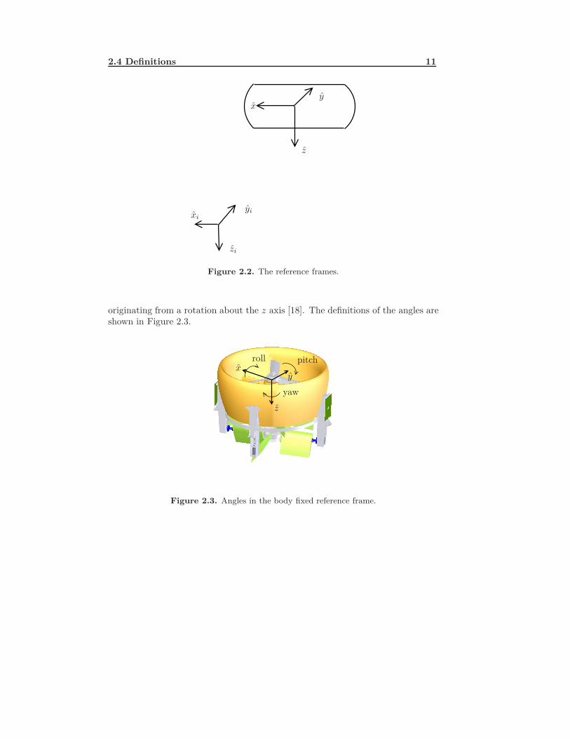
2.4 DefinitionsBefore a mathematical model of the craft can be constructed, reference frames andangles need to be defined. Two reference frames will be used, the inertial referenceframe and the body fixed reference frame. The inertial reference frame has itsorigin fixed to the ground and the body fixed reference frame has its origin fixedin the center of gravity of the craft. Both reference frames are shown in Figure2.2, where the coordinates with index i are the coordinates in the inertial referenceframe. Since the craft is almost symmetrical about the z axis, a direction for oneof the x or y axes has to be defined to obtain a completely defined body fixedreference frame. The x axis is defined as the axis between the center of the craftand one of the control card and the z axis is the axis pointing downwards.
The interesting angles when creating the control system for the craft are theangles in the body fixed reference frame. The body fixed angles are called pitch,roll and yaw and are the angles usually used when the rotation of an aircraft isdescribed. Pitch is the angle originating from a rotation about the y axis, rollis the angle originating from a rotation about the x axis and yaw is the angle
2.4 Definitions 11
xy
z
xiyi
zi
Figure 2.2. The reference frames.
originating from a rotation about the z axis [18]. The definitions of the angles areshown in Figure 2.3.
xy
z
roll pitch
yaw
Figure 2.3. Angles in the body fixed reference frame.

12 Theory
Chapter 3
Rig
3.1 Modifying the Test RigA test rig is a construction where the craft can be placed to simulate a naturalenvironment and to perform controlled tests. A wish from DST Control AB is theconstruction of a new test rig allowing more advanced testing of the craft.
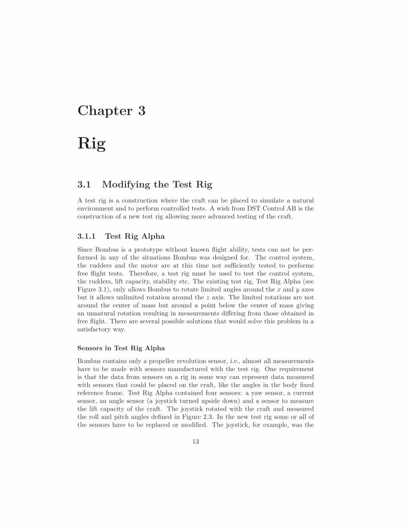
3.1.1 Test Rig AlphaSince Bombus is a prototype without known flight ability, tests can not be per-formed in any of the situations Bombus was designed for. The control system,the rudders and the motor are at this time not sufficiently tested to performefree flight tests. Therefore, a test rig must be used to test the control system,the rudders, lift capacity, stability etc. The existing test rig, Test Rig Alpha (seeFigure 3.1), only allows Bombus to rotate limited angles around the x and y axesbut it allows unlimited rotation around the z axis. The limited rotations are notaround the center of mass but around a point below the center of mass givingan unnatural rotation resulting in measurements differing from those obtained infree flight. There are several possible solutions that would solve this problem in asatisfactory way.
Sensors in Test Rig Alpha
Bombus contains only a propeller revolution sensor, i.e., almost all measurementshave to be made with sensors manufactured with the test rig. One requirementis that the data from sensors on a rig in some way can represent data measuredwith sensors that could be placed on the craft, like the angles in the body fixedreference frame. Test Rig Alpha contained four sensors: a yaw sensor, a currentsensor, an angle sensor (a joystick turned upside down) and a sensor to measurethe lift capacity of the craft. The joystick rotated with the craft and measuredthe roll and pitch angles defined in Figure 2.3. In the new test rig some or all ofthe sensors have to be replaced or modified. The joystick, for example, was the
13

14 Rig
Figure 3.1. Test Rig Alpha.
reason that the craft did not rotate around its center of mass in Test Rig Alpha.The craft rotated around the point where the joystick was fixed in the craft. Theyaw sensor was placed at the end of the joystick, under the craft, and measuredthe rotation of the stick. This means that it only measured the actual yaw anglewhen both roll and pitch angles were zero. To get the actual yaw angle at all timesthe values from the joystick must be combined with the yaw sensor in some way.
3.1.2 Tethers with slackOne solution would be to connect the craft to tethers with slack so that it couldmove freely but a limited distance. The solution has several disadvantages makingit less suitable as test rig at this time. Bombus is designed to have angle andvelocity sensors mounted on the duct but these sensors are at this time not avail-able. The sensors currently used must be placed on the test rig. Mounting highprecision sensors on a test rig based on tethers with slack is close to impossible.Another disadvantage is the relative lack of safety. The craft would in this testrig be loosely tethered which puts high demands on the control system and therudder performance. The tethered test rig also has some advantages like a naturaltest situation.
3.1.3 GimbalAnother solution is to place the craft in the center of a gimbal with the gimbal’saxes through the center of mass of the craft. In a gimbal construction there arethree rotations normaly made possible by two or three rings. In this case two ringswill be used. The first rotation is the outer ring rotating around one inertial axis.The second rotation is the inner ring rotating around the axle rotating with the
3.2 Building Test Rig Beta 15
outer ring. The last rotation is the craft rotating around the axle rotating with theinner ring. All three rotations are perpendicular to the rotation closest in order.This construction will allow the craft to rotate freely around all its axes and stillbe enough tied down to avoid crashing or flying away if the control system failsto keep it stable. The gimbal construction has been used in this way by NASAto train astronauts [7]. The astronauts were strapped were the craft is plannedto be placed and then rotated around all axes to simulate, among other things, aspace craft spin. The only clear drawback with the gimbal test rig is that at onepoint the number of degrees of freedom is two, instead of three, occuring when thetwo rings are aligned. Hopefully this will not cause any problems since the controlsystem should prevent the craft from turning to large angles.
Sensors in the Gimbal Test Rig
If all the rings in the gimbal are horizontal there should not be a problem tomeasure lift capacity. The construction can be done in a way that allows the craftto move vertically within a boundary, when that is required (for example, the axlecan be attached to the craft in vertical tracks allowing the craft to move freelywhen it is not fixed). With the gimbal rings fixed the lift capacity can be measuredwith for example a Newton meter or the existing lift capacity sensor.
There is no easy way to measure the roll, pitch and yaw angles directly for acraft mounted in a gimbal. However, there is no problem measuring the rotationsof the gimbal rings using for example potentiometers measuring the rotation aboutthe three axes. The three dimensions of rotation of the craft can be described as aquaternion calculated from the gimbal angles [13]. From the quaternion the bodyfixed angles are obtained as
rollpitchyaw
=
arctan(
2(q0q1+q2q3)q20−q21−q22+q23
)arcsin (2(q0q2 − q1q3))arctan
(2(q1q2+q0q3)q20+q21−q22−q23
) (3.1)
where q0, q1, q2 and q3 represents the coefficients in the quaternion Q = q0 + iq1 +jq2 +kq3 [22]. Appendix A gives a detailed description of how to get the roll, pitchand yaw angles from gimbal angles using quaternions.
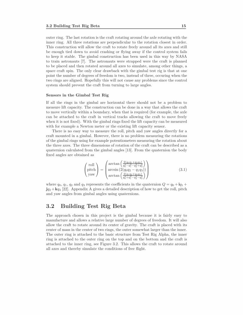
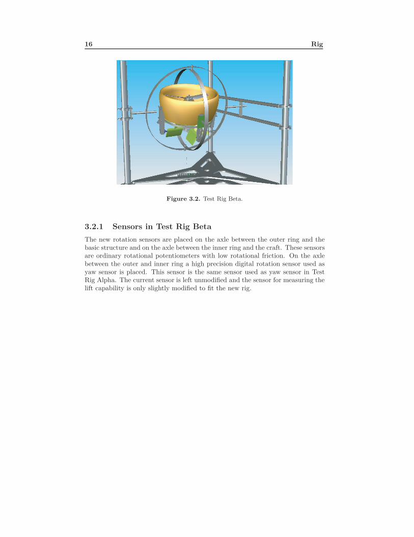
3.2 Building Test Rig BetaThe approach chosen in this project is the gimbal because it is fairly easy tomanufacture and allows a relative large number of degrees of freedom. It will alsoallow the craft to rotate around its center of gravity. The craft is placed with itscenter of mass in the center of two rings, the outer somewhat larger than the inner.The outer ring is attached to the basic structure from Test Rig Alpha, the innerring is attached to the outer ring on the top and on the bottom and the craft isattached to the inner ring, see Figure 3.2. This allows the craft to rotate aroundall axes and thereby simulate the conditions of free flight.
16 Rig
Figure 3.2. Test Rig Beta.
3.2.1 Sensors in Test Rig BetaThe new rotation sensors are placed on the axle between the outer ring and thebasic structure and on the axle between the inner ring and the craft. These sensorsare ordinary rotational potentiometers with low rotational friction. On the axlebetween the outer and inner ring a high precision digital rotation sensor used asyaw sensor is placed. This sensor is the same sensor used as yaw sensor in TestRig Alpha. The current sensor is left unmodified and the sensor for measuring thelift capability is only slightly modified to fit the new rig.

Chapter 4
Lift capacity
One of the most important characteristics of an UAV is its lift capacity. Withoutsufficient lift capacity, the UAV will not be able to lift any equipment. Bombuswas designed primarily for surveillance which often means that a camera has to belifted. In addition to this, Bombus has to lift the tethering cable, including bothpower supply cable and possibly also a data cable.
4.1 Optimal LiftThe lift calculated in this section is optimal in that sense that it only considers thearea of the propeller disc and the power of the engine and not the design of thepropeller blades. This corresponds to the lift generated by an optimal propeller.
4.1.1 Initial CalculationsThese calculations are based on basic aerodynamics and fluid mechanics. A fun-damental rule is that the mass flow into the control volume in Figure 4.1 [14] mustbe the same as the mass flow out of it:∮
S
ρV · dS = 0 (4.1)
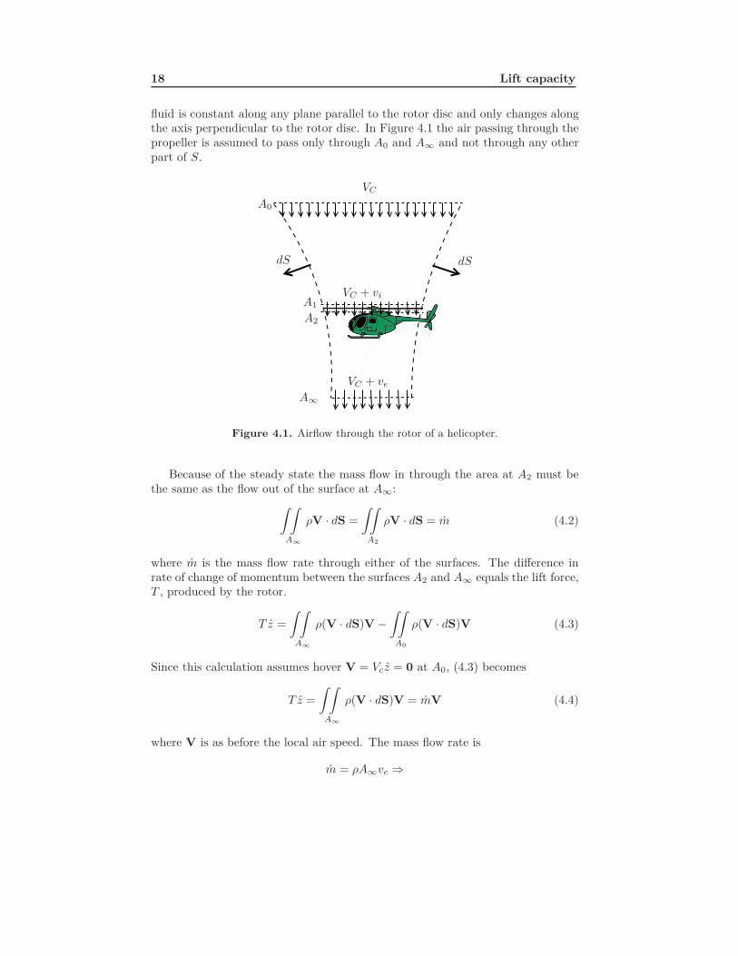
where V is the local velocity of the air, ρ is the density of air and S is the surfaceenclosing the propeller in Figure 4.1, including A0 and A∞. In the followingcalculations V = |V | · (0, 0, 1)T since the air speed can be assumed to have only acomponent downwards. The interesting property to calculate is the lift in hover,meaning that VC in Figure 4.1 is zero. Some other assumptions are made tosimplify the calculations: the fluid (here the gas air) is incompressible, inviscid,one dimensional and the flow is in a quasi-steady state. The assumption that theair is incompressible results in a constant air density. This assumption can bemade since the air can move free and will not be compressed against anything.The assumption that the fluid is one dimensional means that the properties of the
17
18 Lift capacity
fluid is constant along any plane parallel to the rotor disc and only changes alongthe axis perpendicular to the rotor disc. In Figure 4.1 the air passing through thepropeller is assumed to pass only through A0 and A∞ and not through any otherpart of S.
VC
dSdS
A0
A1
A2
A∞
VC + vi
VC + ve
Figure 4.1. Airflow through the rotor of a helicopter.
Because of the steady state the mass flow in through the area at A2 must bethe same as the flow out of the surface at A∞:∫ ∫
A∞
ρV · dS =∫∫A2
ρV · dS = m (4.2)
where m is the mass flow rate through either of the surfaces. The difference inrate of change of momentum between the surfaces A2 and A∞ equals the lift force,T , produced by the rotor.
T z =∫ ∫A∞
ρ(V · dS)V −∫∫A0
ρ(V · dS)V (4.3)
Since this calculation assumes hover V = Vcz = 0 at A0, (4.3) becomes
T z =∫ ∫A∞
ρ(V · dS)V = mV (4.4)
where V is as before the local air speed. The mass flow rate is
m = ρA∞ve ⇒
4.1 Optimal Lift 19
T z = mV = ρA∞veV = ρA∞v2e z = mvez (4.5)
A∞ and ve are the area and air velocity of the control surface at A∞, respectively.The power of the rotor is calculated as P = T |V | giving P = Tvi at the propeller.
P = Tvi =∫ ∫A∞
12ρ(V · dS)V2 −
∫∫A0
12ρ(V · dS)V2 (4.6)
Like above the last integral in (4.6) is zero, because the rotor is in hover. This,together with (4.5), gives
P = Tvi =∫ ∫A∞
12ρ(V · dS)V2 =
12mv3
e =12Tve ⇒ vi =
12ve (4.7)
Because of the symmetry in Figure 4.1, ρA∞w = ρAvi. This combined with theresult in (4.7) gives
ρA∞w = ρAvi ⇒ A∞w = A12w ⇒ 2A∞ = A (4.8)
Since A = πR2 it follows that T = 2ρπR2v2i and P = 2ρπR2v3
i
4.1.2 Calculating the LiftThe rotor disc is the two dimensional surface the air has to pass through to pass therotor. This area is A = πR2, where R is the radius of the rotor. Since the motormounted on Bombus is an electric motor the power is calculated from P = UIewhere U is the voltage, I is the current and e is the efficiency of the motor. Theprevious section resulted in
T = 2ρπR2v2i (4.9)
P = 2ρπR2v3i (4.10)
Calculating v2i from (4.10) gives
v2i =
(P
2ρπR2
) 23
(4.11)
Inserting (4.11) in (4.9) results in an expression for the lift, T , independent of vi
T = 2ρπR2
(P
2ρπR2
) 23
= (2πρR2P 2)13 (4.12)
This result allows the calculation of vi which can be useful when calculating forexample the effect of the guiding vanes and the effect of the rudders used forsteering.
20 Lift capacity
α
φ
θ
Ω
dFL
dFDdFx
dFzdR
dM
U
U
UT
UT
UP
UR
R0
R1
y
Figure 4.2. Legths, velocities and angles in BET.
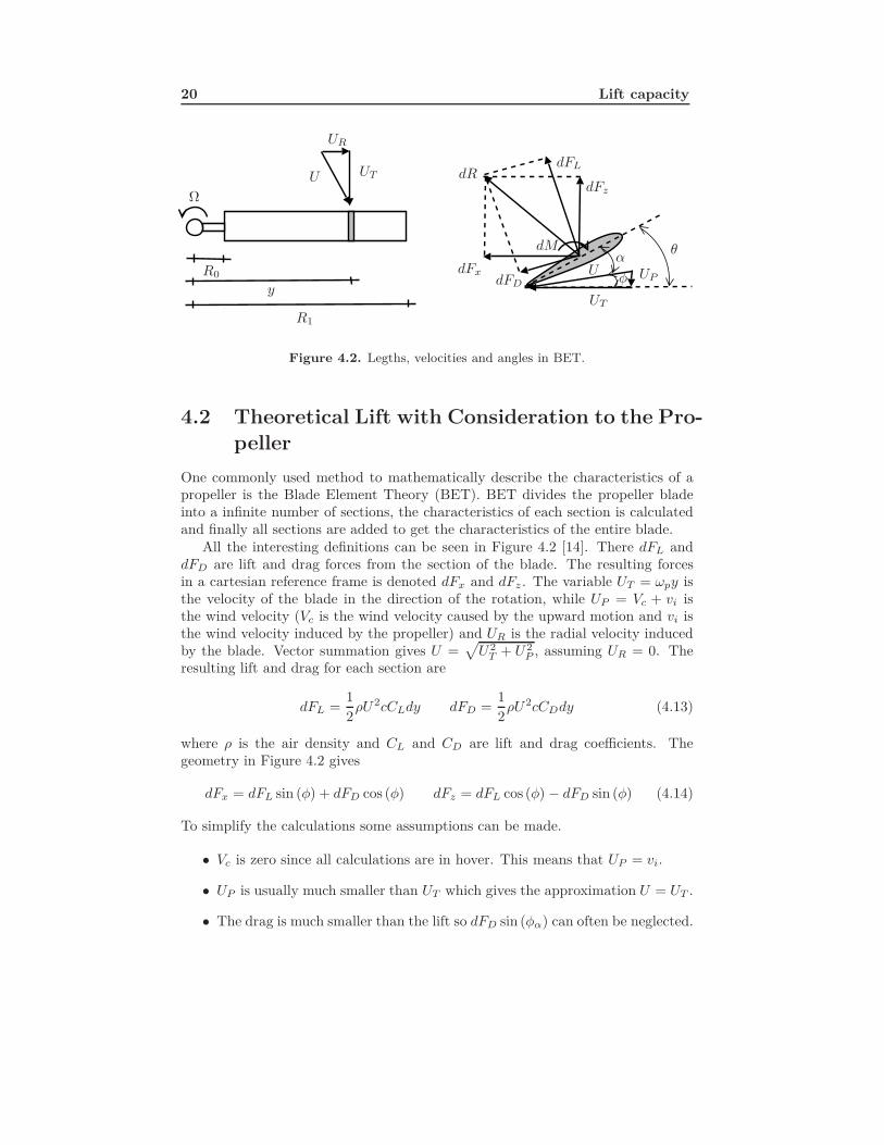
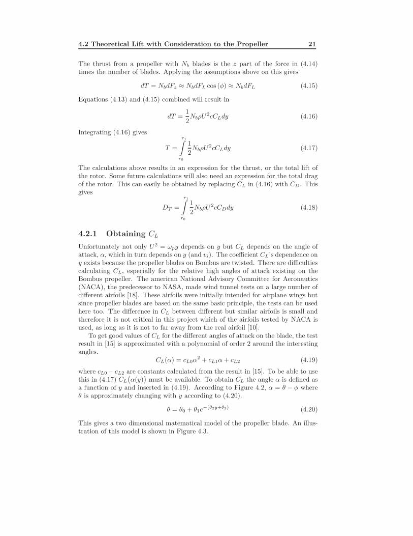
4.2 Theoretical Lift with Consideration to the Pro-peller
One commonly used method to mathematically describe the characteristics of apropeller is the Blade Element Theory (BET). BET divides the propeller bladeinto a infinite number of sections, the characteristics of each section is calculatedand finally all sections are added to get the characteristics of the entire blade.
All the interesting definitions can be seen in Figure 4.2 [14]. There dFL anddFD are lift and drag forces from the section of the blade. The resulting forcesin a cartesian reference frame is denoted dFx and dFz . The variable UT = ωpy isthe velocity of the blade in the direction of the rotation, while UP = Vc + vi isthe wind velocity (Vc is the wind velocity caused by the upward motion and vi isthe wind velocity induced by the propeller) and UR is the radial velocity inducedby the blade. Vector summation gives U =
√U2T + U2
P , assuming UR = 0. Theresulting lift and drag for each section are
dFL =12ρU2cCLdy dFD =
12ρU2cCDdy (4.13)
where ρ is the air density and CL and CD are lift and drag coefficients. Thegeometry in Figure 4.2 gives
dFx = dFL sin (φ) + dFD cos (φ) dFz = dFL cos (φ) − dFD sin (φ) (4.14)
To simplify the calculations some assumptions can be made.
• Vc is zero since all calculations are in hover. This means that UP = vi.
• UP is usually much smaller than UT which gives the approximation U = UT .
• The drag is much smaller than the lift so dFD sin (φα) can often be neglected.
4.2 Theoretical Lift with Consideration to the Propeller 21
The thrust from a propeller with Nb blades is the z part of the force in (4.14)times the number of blades. Applying the assumptions above on this gives
dT = NbdFz ≈ NbdFL cos (φ) ≈ NbdFL (4.15)
Equations (4.13) and (4.15) combined will result in
dT =12NbρU
2cCLdy (4.16)
Integrating (4.16) gives
T =
r1∫r0
12NbρU
2cCLdy (4.17)
The calculations above results in an expression for the thrust, or the total lift ofthe rotor. Some future calculations will also need an expression for the total dragof the rotor. This can easily be obtained by replacing CL in (4.16) with CD. Thisgives
DT =
r1∫r0
12NbρU
2cCDdy (4.18)
4.2.1 Obtaining CL
Unfortunately not only U2 = ωpy depends on y but CL depends on the angle ofattack, α, which in turn depends on y (and vi). The coefficient CL’s dependence ony exists because the propeller blades on Bombus are twisted. There are difficultiescalculating CL, especially for the relative high angles of attack existing on theBombus propeller. The american National Advisory Committee for Aeronautics(NACA), the predecessor to NASA, made wind tunnel tests on a large number ofdifferent airfoils [18]. These airfoils were initially intended for airplane wings butsince propeller blades are based on the same basic principle, the tests can be usedhere too. The difference in CL between different but similar airfoils is small andtherefore it is not critical in this project which of the airfoils tested by NACA isused, as long as it is not to far away from the real airfoil [10].
To get good values of CL for the different angles of attack on the blade, the testresult in [15] is approximated with a polynomial of order 2 around the interestingangles.
CL(α) = cL0α2 + cL1α + cL2 (4.19)
where cL0 – cL2 are constants calculated from the result in [15]. To be able to usethis in (4.17) CL
(α(y)
)must be available. To obtain CL the angle α is defined as
a function of y and inserted in (4.19). According to Figure 4.2, α = θ − φ whereθ is approximately changing with y according to (4.20).
θ = θ0 + θ1e−(θ2y+θ3) (4.20)
This gives a two dimensional matematical model of the propeller blade. An illus-tration of this model is shown in Figure 4.3.

22 Lift capacity
Figure 4.3. Mathematical model of the propeller blade.
The variables θ0 – θ3 in (4.20) are constants calculated from measurementson the propeller. To get a good approximation of φα, vi can be approximated asvi = λhωpy. This fact together with the relation UT = ωpy and geometry fromFigure 4.2 gives
φα = arctanλh (4.21)
Even though λh at this time is unknown it can be written as λh =√
CT
2 . Thisdoes not help since CT has not yet been calculated and depends on T . To solve theproblem all calculations have to be iterated and will then converge to the correctvalue.
With help from (4.19), α = θα−φα, (4.20) and (4.21), the lift can be calculated.
T =12Nbρω
2pc
r1∫r0
y2CLdy =
=12Nbρω
2pc
r1∫r0
y2(cL0(θ0 + θ1e−(θ2y+θ3) − arctan (λh))2+
+ cL1(θ0 + θ1e−(θ2y+θ3) − arctan (λh)) + cL2)dy (4.22)
To calculate the total drag CD is used instead of CL. The NACA wind tunneltests also gave values for CD which can be approximated by a linear function forthe interesting angles. This means that CD(α) = l1α + l2. Using this in (4.20) –(4.22) gives an expression for the total drag.
4.3 Lift Experiments 23
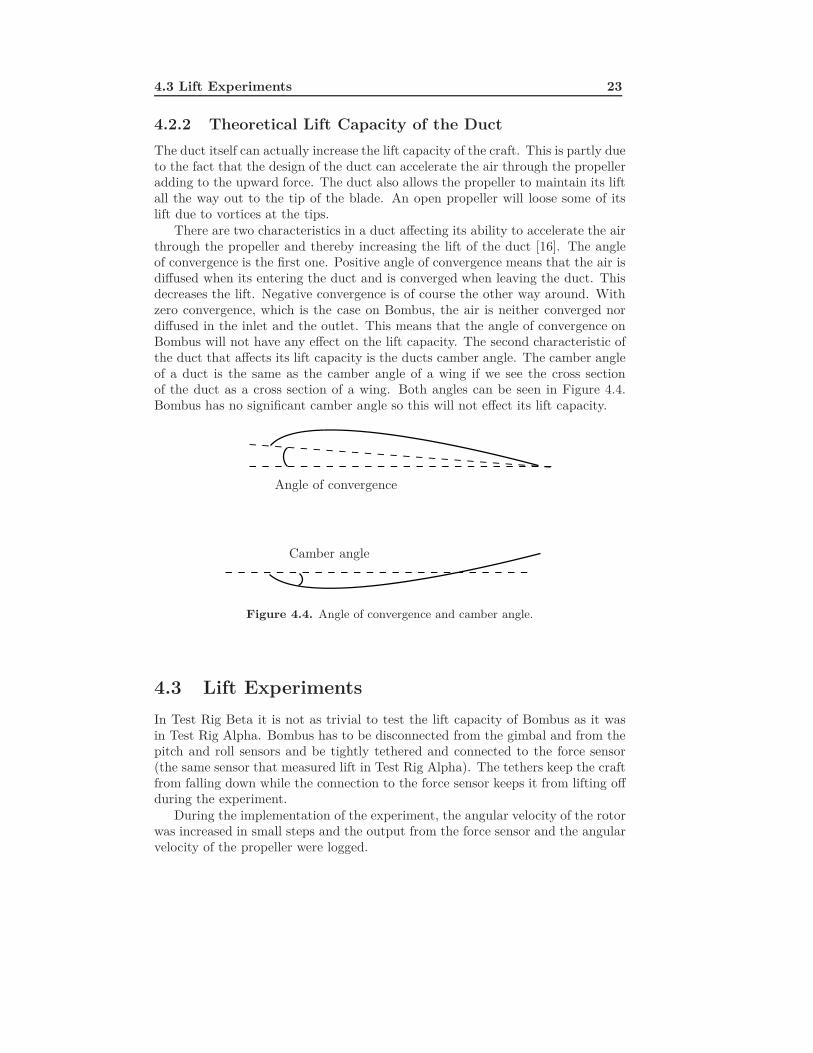
4.2.2 Theoretical Lift Capacity of the DuctThe duct itself can actually increase the lift capacity of the craft. This is partly dueto the fact that the design of the duct can accelerate the air through the propelleradding to the upward force. The duct also allows the propeller to maintain its liftall the way out to the tip of the blade. An open propeller will loose some of itslift due to vortices at the tips.
There are two characteristics in a duct affecting its ability to accelerate the airthrough the propeller and thereby increasing the lift of the duct [16]. The angleof convergence is the first one. Positive angle of convergence means that the air isdiffused when its entering the duct and is converged when leaving the duct. Thisdecreases the lift. Negative convergence is of course the other way around. Withzero convergence, which is the case on Bombus, the air is neither converged nordiffused in the inlet and the outlet. This means that the angle of convergence onBombus will not have any effect on the lift capacity. The second characteristic ofthe duct that affects its lift capacity is the ducts camber angle. The camber angleof a duct is the same as the camber angle of a wing if we see the cross sectionof the duct as a cross section of a wing. Both angles can be seen in Figure 4.4.Bombus has no significant camber angle so this will not effect its lift capacity.
Angle of convergence
Camber angle
Figure 4.4. Angle of convergence and camber angle.
4.3 Lift ExperimentsIn Test Rig Beta it is not as trivial to test the lift capacity of Bombus as it wasin Test Rig Alpha. Bombus has to be disconnected from the gimbal and from thepitch and roll sensors and be tightly tethered and connected to the force sensor(the same sensor that measured lift in Test Rig Alpha). The tethers keep the craftfrom falling down while the connection to the force sensor keeps it from lifting offduring the experiment.
During the implementation of the experiment, the angular velocity of the rotorwas increased in small steps and the output from the force sensor and the angularvelocity of the propeller were logged.

24 Lift capacity
4.4 Comparing Theory and ExperimentsIn the sections above, the theoretical lift of the craft has been calculated in twoways. To be able to decide which of the two theoretical lifts to implement in themathematical model both theoretical results have to be compared to experimentalresults. The result of the lift experiments compared to the theoretical results areshown in Figure 4.5. The dots are the result from the experiments, the dashed lineis the optimal lift and the solid line is the theoretical lift with consideration to thepropeller. The reason that the experimental results show a higher but constantlift for low engine speeds is that the lift force sensor only registers forces largerthan the force required for the craft to take off.
4.4.1 Comparison for Optimal LiftThe calculations of the optimal lift resulted in a larger lift capacity than themeasured one. There can be several reasons for this difference, like the optimalpropeller in the calculations is better than the propeller on Bombus in many ways.For example, the theoretical propeller does not have the limitation of a finitenumber of blades. Despite the limitations, the difference between the theoreticaland measured lift capacity is not very large which indicates that the propeller onBombus, in combination with the duct, is rather effective.
Force
Propeller speed
Figure 4.5. Lift force. Experimental results as dots. Optimal lift force as a dashed lineand theoretical lift force with consideration to the propeller as a solid line.
4.4.2 Comparison for Lift with Consideration to the Pro-peller
The theoretical lift is just like in the case of optimal lift, somewhat larger thanthe experimental results. This difference is due to several reasons. For example,
4.5 Alternative Engines 25
the tools used to measure sizes and angles are rather poor and have a resolutionof about 0.005 m. Other things that may affect the experimental lift is drag dueto angle of attack of the rudders and other things in the airflow’s way. In Figure4.5, the lines representing the theoretical results show a much smaller lift for lowengine speeds. This is due to the force sensor and the problem is explained in thebeginning of Section 4.4.
4.5 Alternative EnginesThe electric motor used in Bombus is a brushless electric DC motor intendedprimarily for model aircraft. A motor better suited for Bumbus must above allhave a higher power to weight ratio. The Bombus motor has a maximum powerto weight ratio of about 1.5 kW
kg . Many of the more powerful electric motors havesignificant higher power to weight ratio but they need a higher voltage to operatewhich puts high demands on the power supply arrangement. One alternative is touse electric AC motors. These also put high demands on the power supply unitsbut can have a power to weight ratio of over 2. The high performance AC motorsare large and heavy and are therefore not suited for Bombus.
Another alternative is a combustion engine which can have a power to weightratio higher than 2 but which have some other drawbacks. Combustion enginesuse some kind of fuel which must be lifted by the craft This fact will limit theflight time to that allowed by the fuel tank and reducing the crafts ability to carryequipment other than fuel. With an electric engine the craft can potentially havea infinite flight time if the power cable is connected to an infinite power source.

26 Lift capacity
Chapter 5
Rudder Performance
An important quality needed for an UAV like Bombus is the ability to controltilting in any direction, i.e., roll or pitch, while airborne. If Bombus should tiltduring flight it would cause it to change the direction of the force induced by thepropeller. This would not only cause the craft to lose lift force but it would alsoresult in a horizontal force. This is not desirable unless the craft is supposed tomove in a horizontal direction or if there is an external force, caused by for examplewind, to be counteracted.
Bombus should also be able to avoid rotating around the vertical axis, yawrotation. The propeller blades do not only generate vertical ”lift” forces but alsohorizontal ”drag” forces. These forces induces a torque which should result ina yaw rotation of the craft. This rotation would be contrary to the propeller’srotation and cause the propeller to rotate slower in the inertial frame. This wouldlead to reduced lift force due to lower velocity of the propeller blades. See Chapter4.
Bombus is equipped with eight rudders assembled to the craft like a star cov-ering the outlet of the duct. These rudders are fixed in a small angle to generatetangential forces counteracting the torque from the propeller blades drag forces.These rudders will be referred to as the guiding vanes.
Bombus is also equipped with four controllable rudders. These rudders areplaced under the craft. The controllable rudders are oriented in pairs at a rightangle to eachother, like a cross. This means that there are two rudders for con-trolling roll and two for controlling pitch. Obviously all four rudders can be usedtogether to generate tangential forces in a similar manner as the guiding vanes.
5.1 Theoretical Force Generated by a RudderThe theories of rudder forces is the same theories as used in Chapter 4 but simplerin some aspects. The rudders are not twisted at all, that is, the angle of attack isconstant over the rudders when the craft is not rotating. The craft not rotating canbe compared to hovering in lift force calculations while rotation can be comparedto climb or descent operations. When this occurs the rudders can be divided into
27
28 Rudder Performance
a infinite number of sections, all behaving like wings climbing or descending witha velocity proportional to the distance to the rotation center.
dFD
dFL
dFx
dFz
α
θα
φα
UP
UT
U
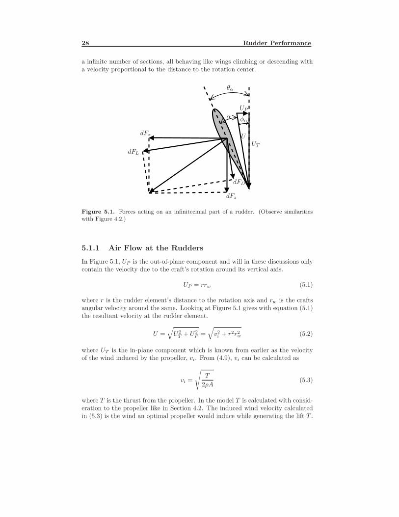
Figure 5.1. Forces acting on an infinitecimal part of a rudder. (Observe similaritieswith Figure 4.2.)
5.1.1 Air Flow at the RuddersIn Figure 5.1, UP is the out-of-plane component and will in these discussions onlycontain the velocity due to the craft’s rotation around its vertical axis.
UP = rrw (5.1)
where r is the rudder element’s distance to the rotation axis and rw is the craftsangular velocity around the same. Looking at Figure 5.1 gives with equation (5.1)the resultant velocity at the rudder element.
U =√
U2T + U2
P =√
v2i + r2r2
w (5.2)
where UT is the in-plane component which is known from earlier as the velocityof the wind induced by the propeller, vi. From (4.9), vi can be calculated as
vi =
√T
2ρA(5.3)
where T is the thrust from the propeller. In the model T is calculated with consid-eration to the propeller like in Section 4.2. The induced wind velocity calculatedin (5.3) is the wind an optimal propeller would induce while generating the lift T .
5.1 Theoretical Force Generated by a Rudder 29
5.1.2 Rudder AnglesThe variable θα represents the rudders angle relative the vertical plane. Theeffective angle of attack is denoted α. As seen in Figure 5.1 the relation is
α = θα − φα (5.4)
whereφα = tan−1
(UP
UT
)(5.5)
Here UP is expected to be small compared to vi which lets (5.5) be approximatedas
φα =UP
UT(5.6)
Combining (5.1), (5.4) and (5.6) gives an expression for the effective angle ofattack.
α = θα − rwr
vi(5.7)
5.1.3 Rudder Forces using Blade Element TheoryIn analogy with Chapter 4 (see in particular (4.13)), the resulting lift and drag foreach section of the rudder are
dFL =12ρU2cCLdr dFD =
12ρU2cCDdr (5.8)
using the rather awkward notation FL (lift) for the force pulling the rudder side-ways and FD (drag) for the force working more close to vertical than horizontal.This notation is used because of the metaphoric image of the rudder element as awing. In (5.8) CL and CD are the rudder’s lift and drag coefficients as a wing. Theparameter ρ is the air density and c is the cord of the rudder. Again in analogywith Chapter 4 looking at Figure 5.1 gives the horizontal and vertical componentsof the force working at the rudder section.
dFz = dFL sin (φα) − dFD cos (φα) dFx = dFL cos (φα) − dFD sin (φα) (5.9)
Combining this with (5.2), (5.6) and (5.8) gives
dFz =12ρc[v2
i + r2r2w]
[CL sin
(rrwvi
)− CD cos
(rrwvi
)]dr (5.10)
dFx =12ρc[v2
i + r2r2w ]
[CL cos
(rrwvi
)− CD sin
(rrwvi
)]dr (5.11)
CL and CD can for the interesting angles be approximated as
CL = cL0α = cL0
(θα − rrw
vi
)(5.12)
30 Rudder Performance
and
CD = cD0 + cD1α + cD2α2 = cD0 + cD1
(θα − rrw
vi
)+ cD2
(θα − rrw
vi
)2
(5.13)
Now dFz and dFx can be integrated over the rudder. With no rotation, r = 0, inparticular
dFz =12ρcv2
i
[CL sin(0) − CD cos(0)
]dr ⇒ Fz =
12ρcv2
i (−CD)
r1∫r0
dr (5.14)
dFx =12ρcv2
i
[CL cos(0) − CD sin(0)
]dr ⇒ Fx =
12ρcv2
iCL
r1∫r0
dr (5.15)
According to [8] the force perpendicular to the wind attacking the rudder is
FL =12ρv2
i SCL(α) (5.16)
which without rotation and when S is the area of the rudder equals Fx in (5.15).
5.2 Theoretical Torque Generated by RuddersThis section discusses the theoretical torque generated by rudders.
5.2.1 Guiding VanesEvery guiding vane generates a torque acting on the vertical central axis of thecraft. From (5.15) the torque generated from every rudder section can be calcu-lated as
dMr = rdFx =12ρcv2
iCLrdr ⇒ Mr =14ρcv2
iCL(r12 − r0
2) (5.17)
The total torque from all guiding vanes is supposed to counteract the torquegenerated from the propellers drag forces. This torque can be calculated using(4.18).
M =12Nbρω
2pcprop
∫blade
y3CD,propdy (5.18)
where ωp is the angular velocity of the fan. This gives the equation
Nr14ρcv2
iCL(αopt)(r12 − r0
2) =12Nbρω
2pcprop
∫blade
y3CD,propdy (5.19)
where αopt is the angle of attack that generates a total torque from the guidingvanes with the same size as the torque generated by the propellers drag forces.
5.3 Rudder Experiments 31
Looking at (5.3) gives v2i = T
2ρA and as seen in (4.22) the thrust from the propellerT ∼ ω2
p. This means that CL(αopt) is independent of ωp. In (5.12) we see that thismeans that αopt is independent of the propellers angular velocity as well (actualangle of the rudder is the same as effective angle of attack due to no yaw rotation).This angle turns out to be small enough not to effect the lifting force noticeably.In more detailed discussions CD in (5.14) is small for the optimal angle of attack.
5.2.2 Controllable RuddersThe purpose of the controllable rudders is to give the control system ability tocontrol torques at all three axes running through the rotational center of the craft.The torque at the vertical axis can be calculated in analogy with (5.17).
Mz,rudder =14ρcv2
iCL(r12 − r0
2) (5.20)
Every rudder generates torques at both horizontal axes. The x component of therudder force generates a torque at the axis parallel with the rudder’s shaft.
dM‖,rudder =12ρcv2
iCLhdr ⇒ M‖,rudder =12ρcv2
iCLh(r1 − r0) (5.21)
where h is the distance from the rudder’s aerodynamic centrum to the axis runningthrough the rotational center of the craft. This is the only difference from (5.15)and (5.21) can be rewritten as
M‖,rudder = hFx (5.22)
The z-component on the other hand generates a torque at the axis perpendicularto the rudder’s shaft. Every rudder section’s force in z direction from (5.14) havethe distance r as lever, giving
dM⊥,rudder =12ρcv2
i (−CD)rdr ⇒ M⊥,rudder =14ρcv2
i (−CD)(r21 − r2
0) (5.23)
But using r21 − r2
0 = (r1 − r0)(r1 + r0) and (5.14) one realise that the torque is therudder’s vertical force with the lever (r1 + r0)/2.
M⊥,rudder =12(r1 + r0)Fz (5.24)
5.3 Rudder ExperimentsThis section describes the experiments made to validate the theoretical torquegenerated by the rudders.
5.3.1 Testing performance of guiding vanesThe guiding vanes are fixed at the optimal angle obtained in (5.19). There areno advanced experiments made to test this configuration. However, it has been
32 Rudder Performance
obvious in all other experiments that these rudders serve their purpose. There hasbeen no rotation around the body fixed z-axis other than when changing angularvelocity of the fan. This rotation is caused by gyral torque (see Section 7.3.3 onpage 44).
5.3.2 Testing Performance of Controllable Rudders
The controllable rudder’s main task is to control the torque about the x and yaxes which will be referred to as tilt torque.
Measuring Tilt Torque in Test Rig Beta
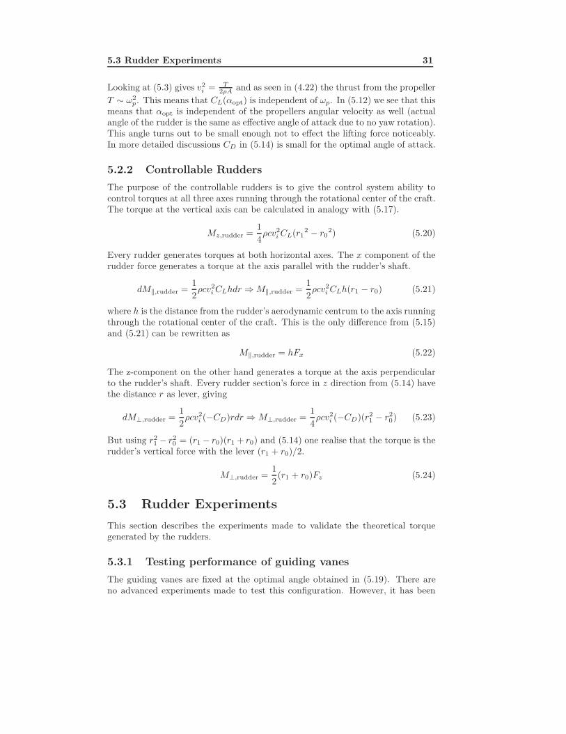
To understand this section the reader should have read Chapter 3 thoroughly. Amethod for measure the torque around one of the horizontal axes was sought. Thiswas obtained by locking the gimbal rings in Test Rig Beta to their initial position.In this way the craft was only allowed to rotate around the axis in which it isassembled to the inner gimbal ring. The sensor earlier used to measure lift forceswas repositioned to be able to measure the vertical force in one leg of the craft.This force levered with the radius of the duct is the torque at the vertical axis.After some testing it was obvious that the sensor reacted when changing fan speedeven if the rudders were in their initial position. Because of the lack of stiffnessin the rig the sensor also measured lift force. The rig was tied down in the craftattachments to avoid this to a certain degree. An illustration of the test rig withthese modification is showed in Figure 5.2.
Figure 5.2. Illustration of Test Rig Beta modified for measuring torque about the y-axis.
5.3 Rudder Experiments 33
Experiment to obtain Characteristics of CL
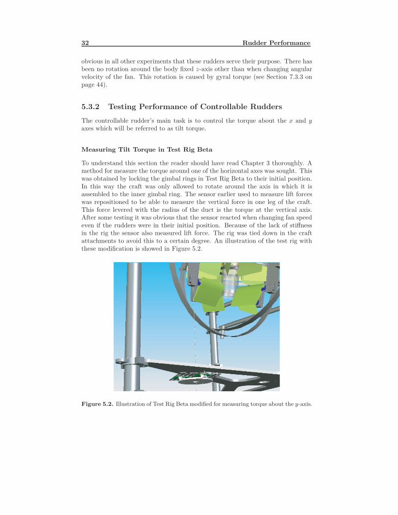
In the theories used, CL is linear for angles smaller than an optimum (see (5.12)).To test these theories the craft’s fan is rotating at a constant speed enough forhovering according to Chapter 4. The angles of the two rudders generating themeasurable torque are varied from a negative angle to a maximal angle far greaterthan the theoretical optimum. A positive angle at these rudders generates a nega-tive torque about the body fixed y-axis. In Figure 5.3 the torque is plotted versusangle of the rudders. The measurement of the torque is rather noisy and it is hard
0
Torque
Angle of attack
Figure 5.3. Torque with two rudders varying angle and fan at constant angular velocity.
to decide whether the relation actually is linear for small angles. However the ex-periments reveal an optimum that agree with the theories. The noise is probablycaused by vortices in the air at the rudders and a rather bad measuring method.The noise will be considered when modeling the rudders in Chapter 7.
Varying propeller speed to verify torque model
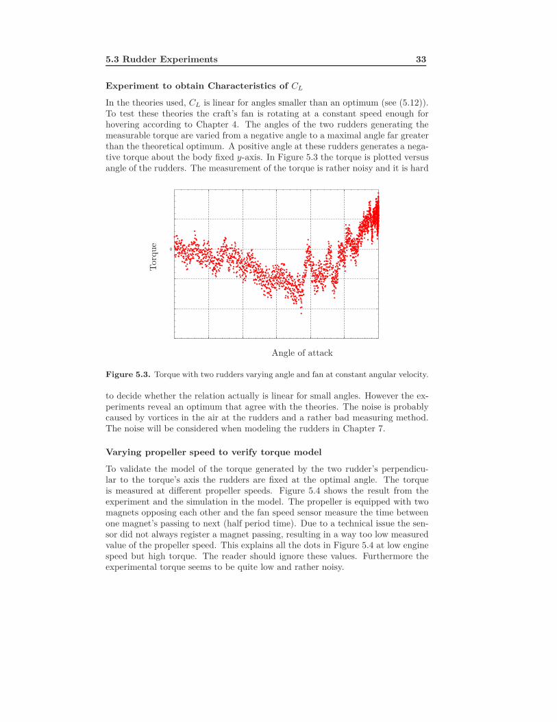
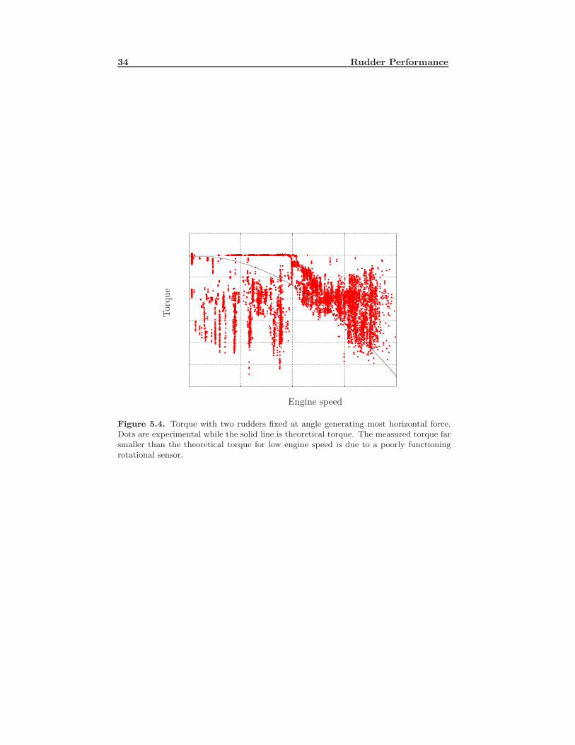
To validate the model of the torque generated by the two rudder’s perpendicu-lar to the torque’s axis the rudders are fixed at the optimal angle. The torqueis measured at different propeller speeds. Figure 5.4 shows the result from theexperiment and the simulation in the model. The propeller is equipped with twomagnets opposing each other and the fan speed sensor measure the time betweenone magnet’s passing to next (half period time). Due to a technical issue the sen-sor did not always register a magnet passing, resulting in a way too low measuredvalue of the propeller speed. This explains all the dots in Figure 5.4 at low enginespeed but high torque. The reader should ignore these values. Furthermore theexperimental torque seems to be quite low and rather noisy.
34 Rudder Performance
Torque
Engine speed
Figure 5.4. Torque with two rudders fixed at angle generating most horizontal force.Dots are experimental while the solid line is theoretical torque. The measured torque farsmaller than the theoretical torque for low engine speed is due to a poorly functioningrotational sensor.
Chapter 6
Noise
Bombus is, as almost every physical system, affected by some kind of noise. Thesources of the noise are often many but in most cases just a few of them affectthe system enough to be needed in a mathematical model. Weather phenomenon,like wind and rain, effects from the ground, like a pull on the tether, wind vorticesbelow the fan and electrical disturbance in wires and control units can all beregarded as sources of noise in this project.
6.1 Weather
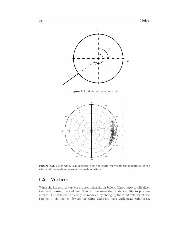
The largest source of noise is the natural wind. Therefore, a mathematical modelof the wind will be inserted into the model of the system. The wind will be modeledas a wind speed from a certain angle. The angle will only be in the xy-plane of theinertial reference frame. This approximation means that the model cannot describewind from above or below. The model of the wind speed will have a certain meanvalue and then low pass filtered white Gaussian noise with mean value zero willbe added to it. This results is a more nature like wind compared to a model withconstant wind speed. Figure 6.1 shows the noise wind and the different angles.Here β is the angle from which the wind arrives, ϕ is the angle to the rudderconsidered in the calculation and vw is the speed of the noise wind. Both anglesequals zero at x. Denote the rudders with numbers, j = 1 . . . 4. Rudder j = 1 isthe rudder at β = 0. This gives an angle to each rudder, ϕj = (j − 1)π/2. Thenoise wind at each rudder becomes
vw,j = vw cos(β − (j − 1)π/2
)(6.1)
The noise wind used in the simulations can be seen in Figure 6.2.Noise sources such as rain and snow will not be modeled since they only occur
in rare situations.
35
36 Noise
2
x
y
vw
ϕ
β
Figure 6.1. Model of the noise wind.
0
330
300
270
240
210
180
150
120
90
60
30
0
Figure 6.2. Noise wind. The distance from the origin represents the magnitude of thewind and the angle represents the angle of attack.
6.2 Vortices
When the fan rotates vortices are created in the air below. These vortices will affectthe wind passing the rudders. This will decrease the rudders ability to producea force. The vortices can easily be modeled by changing the wind velocity at therudders in the model. By adding white Gaussian noise with mean value zero,
6.3 Air Loss 37
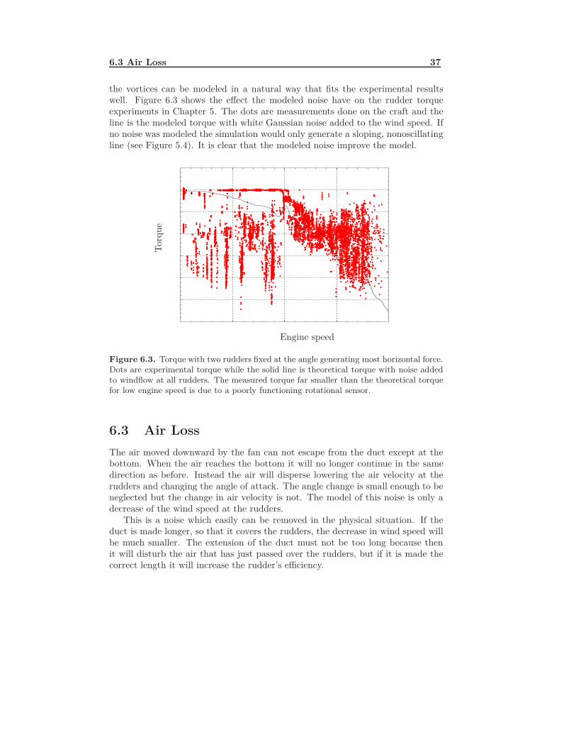
the vortices can be modeled in a natural way that fits the experimental resultswell. Figure 6.3 shows the effect the modeled noise have on the rudder torqueexperiments in Chapter 5. The dots are measurements done on the craft and theline is the modeled torque with white Gaussian noise added to the wind speed. Ifno noise was modeled the simulation would only generate a sloping, nonoscillatingline (see Figure 5.4). It is clear that the modeled noise improve the model.
Torque
Engine speed
Figure 6.3. Torque with two rudders fixed at the angle generating most horizontal force.Dots are experimental torque while the solid line is theoretical torque with noise addedto windflow at all rudders. The measured torque far smaller than the theoretical torquefor low engine speed is due to a poorly functioning rotational sensor.
6.3 Air LossThe air moved downward by the fan can not escape from the duct except at thebottom. When the air reaches the bottom it will no longer continue in the samedirection as before. Instead the air will disperse lowering the air velocity at therudders and changing the angle of attack. The angle change is small enough to beneglected but the change in air velocity is not. The model of this noise is only adecrease of the wind speed at the rudders.
This is a noise which easily can be removed in the physical situation. If theduct is made longer, so that it covers the rudders, the decrease in wind speed willbe much smaller. The extension of the duct must not be too long because thenit will disturb the air that has just passed over the rudders, but if it is made thecorrect length it will increase the rudder’s efficiency.

38 Noise
Chapter 7
Theoretical Model
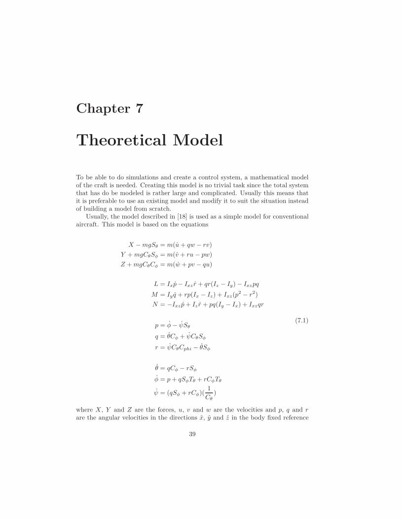
To be able to do simulations and create a control system, a mathematical modelof the craft is needed. Creating this model is no trivial task since the total systemthat has do be modeled is rather large and complicated. Usually this means thatit is preferable to use an existing model and modify it to suit the situation insteadof building a model from scratch.
Usually, the model described in [18] is used as a simple model for conventionalaircraft. This model is based on the equations
X −mgSθ = m(u + qw − rv)Y + mgCθSφ = m(v + ru − pw)Z + mgCθCφ = m(w + pv − qu)
L = Ixp− Ixz r + qr(Iz − Iy) − Ixzpq
M = Iy q + rp(Ix − Iz) + Ixz(p2 − r2)N = −Ixzp + Iz r + pq(Iy − Ix) + Ixzqr
p = φ− ψSθ
q = θCφ + ψCθSφ
r = ψCθCphi − θSφ
θ = qCφ − rSφ
φ = p + qSφTθ + rCφTθ
ψ = (qSφ + rCφ)(1Cθ
)
(7.1)
where X , Y and Z are the forces, u, v and w are the velocities and p, q and rare the angular velocities in the directions x, y and z in the body fixed reference
39
40 Theoretical Model
frame. Torques about x, y and z in the body fixed reference frame are denotedM ,L and N respectively. The Euler angles are denoted φ, θ and ψ, m is the totalmass, g is the gravitational constant and Cθ, Sφ and Tψ are cos (θ), sin (φ) andtan (ψ) respectively. Finally, Ia is the moment of inertia about the axis a where acan be x, y or z in the body fixed reference frame.
7.1 Forces; X, Y and Z
There are four kinds of forces acting on the craft. The first one is the gravity, thesecond one is the lift, the third one is the forces generated by the rudders and thefinal one is the drag generated by the rudders and the duct when the noise windacts on them. The general equation for the forces are therefore
X = Xr2,r4 + Xduct drag + Xrudder drag
Y = Yr1,r3 + Yduct drag + Yrudder drag
Z = −T
(7.2)
where Xr2,r4 is the forces generated by the rudders, Xduct drag is the drag from theduct and Xrudder drag is the drag from the rudders. The reason for not includingthe gravitational force in the third equation in (7.2) is that it is already modeledin (7.1). Xr2,r4 and Yr1,r3 can easily be obtained by calculating the force fromeach rudder, using equation (5.15), and then summarizing all forces acting in eachdirection.
The second term in (7.2) originates from the drag of the duct. According to[8] the drag of a structure can be calculated as
Xduct drag =12ρv2
w cos (β)AdCD,d (7.3)
where Ad is the area of the duct facing the wind, CD,d is the drag coefficient of theduct and β is the angle from the x-axis to the current propeller blade. Accordingto [16] CD, of a smooth cylinder with the same dimensions as Bombus is about 1.
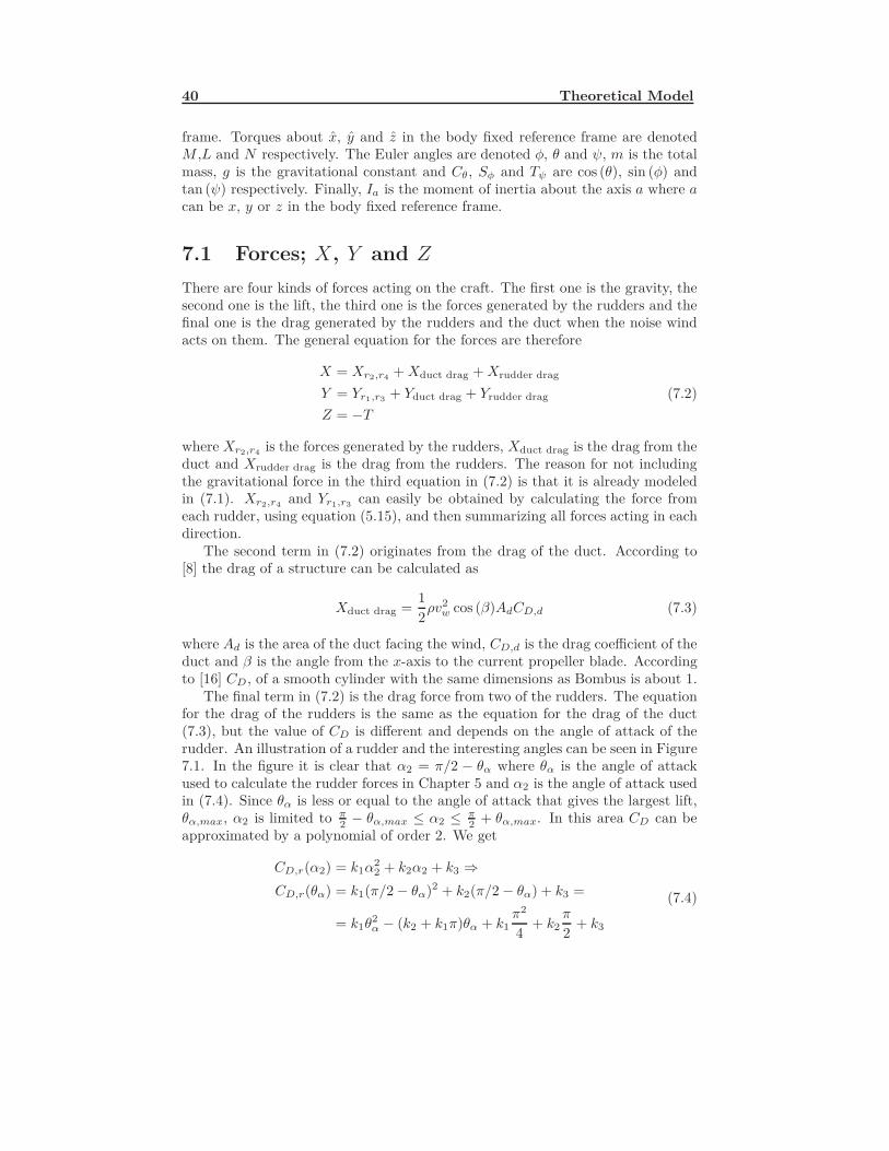
The final term in (7.2) is the drag force from two of the rudders. The equationfor the drag of the rudders is the same as the equation for the drag of the duct(7.3), but the value of CD is different and depends on the angle of attack of therudder. An illustration of a rudder and the interesting angles can be seen in Figure7.1. In the figure it is clear that α2 = π/2 − θα where θα is the angle of attackused to calculate the rudder forces in Chapter 5 and α2 is the angle of attack usedin (7.4). Since θα is less or equal to the angle of attack that gives the largest lift,θα,max, α2 is limited to π
2 − θα,max ≤ α2 ≤ π2 + θα,max. In this area CD can be
approximated by a polynomial of order 2. We get
CD,r(α2) = k1α22 + k2α2 + k3 ⇒
CD,r(θα) = k1(π/2 − θα)2 + k2(π/2 − θα) + k3 =
= k1θ2α − (k2 + k1π)θα + k1
π2
4+ k2
π
2+ k3
(7.4)
7.2 Moment of Inertia, Ia 41
α1
α2
Figure 7.1. Angles of attack of the rudders.
This results in a force
Xrudder drag = 212ρv2
w cos (β)ArCD,r(θα) (7.5)
where CD,r(θα) is described in equation (7.4).If the force from rudder x is denoted Frx the total rudder forces can be written
as
Xr2,r4 = −Fr2 − Fr4
Yr1,r3 = Fr1 − Fr3(7.6)
The sign of the forces in (7.6) depend only on the definition of positive anglefor each ruddder as implemented in the software on the craft. The resulting forcesbecomes
X = −Fr2 − Fr4 +12ρv2
w cos (β)AdCD,d + 212ρv2
w cos (β)ArCD,r(θα)
Y = Fr1 − Fr3 +12ρv2
w sin (β)AdCD,d + 212ρv2
w sin (β)ArCD,r(θα)
Z = −T
(7.7)
7.2 Moment of Inertia, Ia
One important characteristic of the craft is its moment of inertia. The moment ofinertia describes how hard it is to change the crafts velocity. It depends only onthe weight and shape of the body and is calculated as
42 Theoretical Model
Ia =∫ν
r2dm =∫ν
r2ρdν (7.8a)
Iab =∫ν
dadbdm =∫ν
dadbρdν (7.8b)
where a is the axis about which the moment of inertia is calculated, ν is thevolume, ρ is the density of the material in the volume, m is the mass, r is theperpendicular distance to a and da is the distance in the direction of a. Thismeans in practice that the equations are
Ix =∫ν
(y2 + z2)ρdν Ixy = Iyx =∫ν
xyρdν
Iy =∫ν
(x2 + z2)ρdν Ixz = Izx =∫ν
xzρdν
Iz =∫ν
(x2 + y2)ρdν Iyz = Izy =∫ν
yzρdν (7.9)
The total moment of inertia on matrix form is
I =
Ix Ixy Ixz
Iyx Iy IyzIzx Izy Iz
(7.10)
Most parts of the craft can be approximated by two or three dimensional bodies.This simplifies the calculations since both [19] and [20] has lists of different bodiesand their moment of inertia. To get the total moment of inertia about one axisin the body fixed reference frame the moment of inertia for all the different partsabout the axis are added.
7.3 Torques; M , L and N
There are several factors affecting the total torque on Bombus. The rudders,described further in Section 5.2.2, will create torques about all three axis. Anotherfactor affecting the total torque is the wind noise described in Chapter 6. Thiswind will have two different effects. First it will increase the lift on one side ofthe craft and decrease it on the other and second, it will generate a drag forcefrom the rudders resulting in a torque. It will also create a drag force on the ductitself but since the center of gravity of the duct is placed in the center of the duct,this will not create any torque. One futher factor affecting the total torque is thetorque created by the gyroscopic effect of the propeller. The torques of the craftare
L = Lr2+r4 + LD(r1,r3,vw) + Llift + Lgyro
M = Mr1+r3 + MD(r2,r4,vw) + Mlift + Mgyro
N = Nr1,r2,r3,r4 + Ngyro
(7.11)

7.3 Torques; M , L and N 43
where rn is rudder number n, vw is the noise wind and D refers to the drag of therudders. The quantities Lr2+r4 , Mr1+r3 and Nr1,r2,r3,r4 are calculated in Section5.2.2 and the rest will be calculated below.
7.3.1 Drag TorqueThe general expression for the drag torque can be written O = O(ra, rb, h, vw)where h is the perpendicular distance from the crafts center of gravity to thetheoretical location of the force. Using (5.8) the drag from the propeller becomes
FD,r =12ρvw
2ArCD,r (7.12)
where Ar is the rudder area and CD,r is the drag coefficient. The drag coeficientCD,r is determined by the airfoil and the angle of attack. The correct angle isapproximately αrD = π − α where α is the angle of the rudder from its originalposition. From Chapter 6 we have vw = vw(cos (β)x + sin (β)y) which togetherwith the fact that two rudders work in the same direction and (7.12) gives
LD(r2,r4,vw) = 2hv12ρv2
wArCD sin (β)
MD(r2,r4,vw) = 2hv12ρv2
wArCD cos (β)(7.13)
In the equations above, hv is the lever for the torque. It is the perpendicularvertical distance between the center of gravity of the craft and the aerodynamiccenter of the rudder.
7.3.2 Torque due to Difference in LiftThe third terms in (7.11), that is, Llift and Mlift, are not as straight forward tocalculate as the previous terms. The torques Llift and Mlift exist due to the factthat the noise wind is added to the induced wind on one side of the propeller andsubtracted from the induced wind on the opposite side. This gives a larger lift onone of the sides which in turn creates a torque about the x and/or y axis. In thiscase (4.3) will not result in equation (4.4) as in the hover case. If the definitionsin Figure 4.1 are used, the lift can be calculated as
T = ρA∞ve(ve − Vc) (7.14)
Since vi = ve+v02 [16] we get
T = ρAr(Vc + vi)2vi (7.15)
As an example, we calculate the torque about the x-axis, L, with the noise windblowing from the direction where y = 0. In this case the force is
FT = TF+ − TF− = 2ρAr(vw + vi)2vi − 2ρAr(−vw + vi)2vi = 4ρArvwvi (7.16)

44 Theoretical Model
where TF+ is the force on the side where the noise wind is added to the inducedwind and TF− is the side where the noise wind is subtracted from the inducedwind. To calculate the total torque from this force we introduce an angle γ as theangle to an arbitrary part of the rotor disc. Using γ to describe the effect of thewind noise on the induced wind results in
vtot = vi + vw,m cos(γ) (7.17)
where vw,m is the magnitude of the noise wind. Since the noise wind is added toone side and subtracted to the other side, the total lift will not be affected. Thismeans that the total lift still is T = 2ρπR2v2
i . To calculate the length of the lever,the lift per area unit, ρL(r, γ), first has to be calculated. The lift per area unitdepends only on the radius, r, and the introduced angle, γ, and can be calculatedfrom
R∫0
2π∫0
ρL(r, γ)dγdr = 2ρπR2v2 ⇒
⇒ ρL(r, γ) = 2ρrvi(vi + vw,m cos (γ)) (7.18)
The term vw,m cos (γ) in ρL(r, γ) could be any constant times cos (γ), but from(7.17) it follows that vw,m is the correct constant.
The lever is calculated in the same way as the center of mass is calculated in[21].
r =
∫ArρL(r, γ)dA∫
A ρL(r, γ)dA=
=
∫ R
0
∫ 2π
0 2ρr2vi(vi + vw,m cos (γ))dγdr∫ R
0
∫ 2π
0 2ρrvi(vi + vw,m cos (γ))dγdr=
=232πρR3v2
i
2πρR2v2i
=23R (7.19)
Combining (7.16) and (7.19) gives
Llift = 423ρπR3vwvi sin (β)
Mlift = 423ρπR3vwvi cos (β) (7.20)
7.3.3 Torque due to the Rotation of the PropellerThe final term of the equations for L and M in (7.11) are the torques generated bythe rotation of the propeller. These torques can be calculated with the momentof inertia of the rotating parts. According to the definitions in Section 7.2 themoment of inertia for the popeller about the z-axis is
Iz =∫ν
(x2 + y2)ρdν (7.21)
7.3 Torques; M , L and N 45
x
y
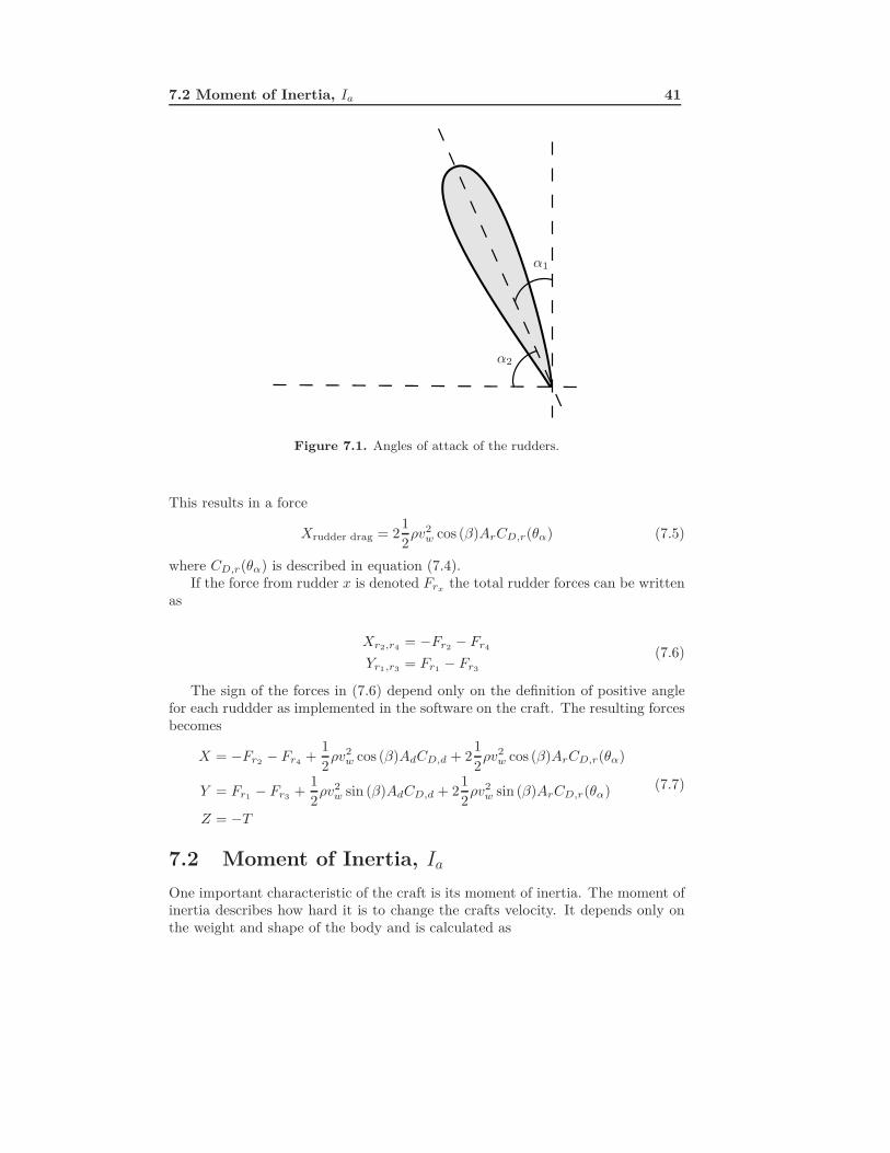
Figure 7.2. A propeller with a arbitrary number of blades.
The propeller in Figure (7.2) has an arbitrary number of blades. They are ap-proximated as two dimensional areas with the length lw and the width bw and areplaced at the angle γ from the x-axis. The moment of inertia for the i:th blade iscalculated as
Iz,i =∫ν
(x2 + y2)ρdν =
cos (γ)lw∫0
aix+bw∫aix−bw
(x2 + y2)ρdydx =
= (13(2bw + 2a2
i bw)(cos (γ)lw)3 − 13b2w cos (γ)L)ρ =
= (13(2 + 2a2
i )(cos (γ))3l2w − 13bw cos (γ))mi
(7.22)
where ai is a constant that together with the width of the blade, bw, describe therelation between x and y for blade i as y = aix + bw or y = aix − bw for the twoedges of the blade. This constant only depends on the angle from the x-axis to thecurrent blade. The mass of blade i is mi = ρlwbw. The total moment of inertiaabout the z-axis is the sum of the moment of inertia for each blade.
Iz =Nb∑i=1
Iz,i (7.23)
The moments of inertia about the x- and y-axis are, in the same way as themoment of inertia about the z-axis, dependent on the angle between the x-axis andthe blade. Since the propeller rotates in the xy-plane of the body fixed reference

46 Theoretical Model
frame the blade that points in the direction of the x-axis at time τ = 0 will pointin the direction of the y-axis at time τ = π/2
ωp(ωp is the angular velocity of the
propeller versus the caft). This means that Ix = Iy when the propeller is rotating.The cross terms of the moment of inertia, Ixy, Ixz and Iyz are zero. The term Ixyis zero because the propeller is symmetrical around the z-axis and Ixz and Iyz arezero because z = 0 in the plane of the propeller. The moments of inertia abovewill result in a torque calculated as
∑M =
(dHG
dt
)xyz
+ Ω× HG (7.24)
where HG = Iω is the angular momentum about the ducts center of gravity, Ωis the angular velocity of the craft and ωp is the angular velocity of the propeller.This means that
Ω =
p
qr
ω =
p
qr + ωp
(7.25)
Inserting (7.25) in (7.24) gives
∑M =
Ix 0 0
0 Iy 00 0 Iz
p
qr + ωp
+
+
p
qr
×
Ix 0 0
0 Iy 00 0 Iz
p
qr + ωp
=
=
Ixp− Iyqr + Izq(r + ωp)
Iy q + Ixpr − Izp(r + ωp)Iz(r + ωp) + Iypq − Ixpq
(7.26)
When Ix = Iy is inserted we get
∑M =
Ixp− Iyqr + Izq(r + ωp)
Iy q + Ixpr − Izp(r + ωp)Iz(r + ωp)
(7.27)
This means that
Lgyro = Ixp− Iyqr + Izq(r + ωp)Mgyro = Iy q + Ixpr − Izp(r + ωp)Ngyro = Iz(r + ωp)
(7.28)
7.4 The Complete Model 47
7.3.4 Resulting Torques
The calculations in the sections above result in the following equations for thetorques
L =h(−Fr1 − Fr3) + 2hv12ρv2
wArCD sin (β)2−
− 423ρπR3vwvi sin (β) + Ixp− Iyqr + Izq(r + ωp)
M =h(Fr1 + Fr3) + 2hv12ρv2
wArCD cos (β)2+
+ 423ρπR3vwvi cos (β) + Iy q + Ixpr − Izp(r + ωp)
N =hh(Fr1 + Fr2 − Fr3 − Fr4) + Iz(r + ωp)
(7.29)
In the equations above, hh is the lever for the torque about the z-axis. This is thehorizontal perpendicular distance between the center of gravity of the duct andthe aerodynamic center of the rudder. In most cases, ωp will be zero but it willresult in a torque that is too big to be neglected when it is not zero. Especiallywhen p is zero, which is the case in most test enviroments, an ωp different fromzero will be clearly noticeable.
7.4 The Complete Model
In the sections above everything but the velocities, angular velocities and Eulerangles have been explained. The variables u, v and w are the velocities of thecraft in the body fixed reference frame and p, q and r are the angular velocities inthe same reference frame. Finally, φ, θ and ψ are the Euler angles. The complete

48 Theoretical Model
model in (7.1) can now be rewritten as
u =X
m− qw + rv − g sin (θ)
v =Y
m− ru + pw + g sin (φ) cos (θ)
w =Z
m− pv + qu + g cos (φ) cos (θ)
p =1Ix
(L − qr(Iz − Iy))
q =1Iy
(M − pr(Ix − Iz))
r =1Ix
(N − pq(Iy − Ix))
φ = p + tan (θ) sin (φ)q + tan (θ) cos (φ)r
θ = cos (φ)q − sin (φ)r
ψ =sin (φ)cos (θ)
q +cos (φ)cos (θ)
r
(7.30)
It is obvious that three equations have disappeared compared to equations (7.1).This is because the six last equations in (7.1) have been combined to create thethree last equations in (7.30). Another mathematical relation used when calculat-ing the model is the relation between the velocities in the inertial reference frameand the velocities in the body fixed reference frame, given by
dxi
dtdyi
dtdzi
dt
=
CθCψ SφSθCψ − CφSψ CφSθCψ + SφSψ
CθSψ SφSθSψ + CφCψ CφSθSψ − SφCψ
−Sθ SφCθ CφCθ
u
vw
(7.31)
7.5 Improving the ModelThe model calculated in the sections above corresponds fairly good to experimentscarried out. However, strange behaviour showed up in longer simulations.
7.5.1 Air ResistanceThe most obvious was that a movement of the craft would continue until a forcefrom the rudders or the noise wind counteracted it, making the system an unstablesystem. Such behaviour is on the real system opposed by air resistance. The airresistance will have the same effect on the craft as a noise wind, generating boththe forces and torques the noise wind does. If the noise wind speed, vw, and theangle of attack of the noise wind, β, is modified with the information about the

7.5 Improving the Model 49
velocity of the craft only small changes have to be made to the model equations.The equations in (7.7) with the modifications becomes
X = −Fr2 − Fr4 +12ρ(v2
w cos (β) − u)AdCD,d + 212ρ(u2 + v2
w cos (β))ArCD,r(α1)
Y = Fr1 − Fr3 +12ρ(v2
w sin (β) − v)AdCD,d + 212ρ(v2 + v2
w sin (β))ArCD,r(α1)
where u and v are the x and y terms of the craft velocity in the body fixed referenceframe.
7.5.2 Twin RuddersExtensive simulations were made to determine the systems resistance to distur-bances, the most important source of disturbance being the noise wind. Thesystem reacted as expected but the forces generated by the rudders was not largeenough to counteract even the slightest noise wind. When two rudders workedat maximum angle to counteract a noise wind of small magnitude the best resultachieved was a state where the craft was stable but with a constant pitch/rollcaused by the noise wind. The rudders were unable to force the craft back toa horizontal position. The insufficient rudder forces generated indicated that thecraft, in particular the rudders, had to be modified to enable the craft to withstanda larger noise wind.
Modification of the Rudders
There are several ways to modify the craft so that the rudders generate a greaterforce and torque. If the lever was to be prolonged the torque would increase butthe force generated by the rudders would not. A better sollution is to find a wayto increase the force without prolonging the lever.
To generate a greater torque by enlarging the lever the rudders must be placedlower or the weight distribution of the craft must be altered so that the centerof gravity of the craft is located higher. Both these solutions result in unwantedeffects like larger torque generated by the noise wind. Placing the rudders lowerwill increase the wanted torque generated by the movement of the rudders butit will also, and for the same reason, increase the torque generated by the dragforce of the rudders caused by the noise wind. The increased noise wind torqueis of course unwanted. If the weight distribution of the craft instead is altered sothat the center of gravity is moved upwards the same effect on both the wantedand unwanted rudder torques is obtained. In addition to these two effects themovement of the center of gravity will result in the need for a more complicatedmathematical model since the modification will cause the center of gravity to beplaced at a point separated from the vertical center of the duct. If the center ofgravity is somewhere else but at the vertical (and horizontal) center of the duct atorque caused by the noise wind’s effect on the duct will occur. This is of courseunwanted.
50 Theoretical Model
To generate a greater torque without enlarging the lever would require largerrudder forces. The force of a rudder is calculated as
FL =12ρv2
iArCL(α)
in Section 5.1.3. This equation means that the force generated by the rudderdepends on the air density ρ, the wind speed induced by the propeller vi, thearea of the rudder Ar, the lift coefficient CL(α) and through the lift coefficientalso on the angle of attack α. The air density is difficult to increase, as is thewind speed induced by the propeller. Both the air density and the air speed isof course possible to change but the simplest way to change any of them wouldbe to change the engine. Changing the engine would require an expensive newengine and many hours of installation work. The angle of attack is the simplestparameter to increase but CL does not have a linear dependence of α and themaximum angle of attack allowed at this point is the angle of attack generatingthe largest CL (and thereby the largest force). There is one angle of attack thatfor some airfoils might give a greater force then the angle the rudders now arerestricted to. This angle is more than twice as big as the angle of restriction andthe larger angle only generates a few per cent more lift, if any. A larger anglehave several disadvantages compared to the restriction angle now used. Since theservos controlling the rudders have a constant maximum turning velocity it willtake longer time for the rudders to reach the larger angle. If two neighboringrudders were to be placed at their maximum angle (the maximum angle being thelarger of the angles discussed) towards each other one rudder would disturb theother both by touch and by disturbing the wind moving over the other rudderwith its own wind.
The only logical way to increase the rudder forces is to increase the rudder area(this might as a secondary effect increase or decrease CL). Increasing the rudderarea will in most cases increase the area exposed to the noise wind which in turnwill increase the drag force due to the noise wind. The increased force and torquedue to the noise wind is unwanted and must be avoided. To increase the rudderarea without increasing the area exposed to the noise wind a twin rudder set upcan be constructed. A schematic description of the twin rudder setup is shown inFigure 7.3. Twin rudders as it looks on Bombus is shown in Figure 7.4.
Even though the twin rudder doubles the rudder area without noticeable in-creasing the drag of the rudder, the twin rudder will not generate twice the forceof the single rudder. This is because of something called the biplane effect. Thename of this effect of course originates from biplanes using the same setup for theirmain wings. The biplane effect is the loss of lift due to the interference betweenthe two wings (or in this case rudders) [17]. To decrease the biplane effect the gapG and the stagger D (see Figure 7.3) can be increased but to completely removethe effect the gap has to be greater than twice the cord, c. On the current set upon Bombus the gap is about 30% of the cord and the stagger varies with the angleof attack but peaks at about 10% of the cord at the maximum angle of attack. InFigure 7.5, the theoretical CL can be seen for the monoplane, the upper biplanewing, the lower biplane wing and the total biplane cellule. Note that Figure 7.5 is

7.5 Improving the Model 51
G
G
D
c
c
vivi
Twin rudders without angle of attack Twin rudders with angle of attack
Figure 7.3. Double rudders.
Figure 7.4. Bombus modified with twin rudders.

52 Theoretical Model
Lower wing
Upper wing
Mono plane
Bi plane
CL
Angle of attack
Figure 7.5. Theoretical appearance of the lift coefficient graph.
not an exact figure but shows the general appearance of the lift coefficient graph.The lift coefficient graph will vary some when parameters like gap, stagger, air-foil and cord varies. Since CL for the biplane is somewhat smaller than CL forthe monoplane and the biplane has a twices as big wing area as the monoplanethe theoretical lift force for the biplane is somewhat less than twice that of themonoplane just as predicted by the biplane effect.
Experimental Performance of Twin Rudders
To determine if the theory regarding the twin rudders and the comparison betweenthe twin rudders and the biplane is correct, experiments had to be carried out.The twin rudder experiments were the same as the torque experiments in Section5.3 but with twin rudders instead of single rudders. The results from one ofthe experiments are shown in Figure 7.6. The light pluses are the results fromthe experiment with a twin rudders and the dark dots are the results from theexperiments with single rudders. It is clear that the torque when using doublerudders is about twice as large as the torque when using single rudders. Withthe double rudders implemented in the mathematical model the simulations showa significant increase in disturbance resistance as well as a behavior more likethe desired when a control system is connected and works to steer the craft toa specific angle or position. An even better effect can be achieved with a largernumber of rudders in the same assembly, for example three instead of two, butthen the biplane effect is increased resulting in a decrease increased torque toincreased weight ratio. Increasing the number of rudders in the same assemblywill also decrease the maximum angle of the rudder assembly before the assemblytouches the neighboring rudder assembly.
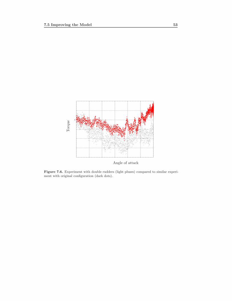
7.5 Improving the Model 53
0
Torque
Angle of attack
Figure 7.6. Experiment with double rudders (light pluses) compared to similar experi-ment with original configuration (dark dots).

54 Theoretical Model
Chapter 8
Control
Almost every modern aircraft uses an advanced control system to assist the pilot.In some cases, like in modern fighter aircraft, the aircraft itself is unstable so thecontrol system is necessary in order to give the pilot ability to fly the aircraft.Other aircraft are designed to be stable making a control system less necessaryeven if a control system still can assist the pilot with tasks like wind correction.Since an UAV has no pilot, the performance of the control system is of largeimportance. If the control system fails an accident is almost inevitable.
To obtain a good control system for Bombus several different control systemswill be tested. Since a mathematical model has been carefully derived a con-trol system based on this model can be implemented. However, a PID controllerindependent of the model will also be implemented.
All controllers will have the same inputs and generate the same outputs. Theinputs are the coordinates in the inertial reference frame and the outputs are theangles of the rudders and the engine speed. If the craft were to be controlled byan operator it is possible that instead of using the three inertial coordinates asreferences, the corrsponding velocities can be used. This gives the operator a morenatural feeling.
8.1 PIDThe PID controller can, despite its simplicity, in many cases be sufficiently effec-tive. The problem when using PID controllers in large systems is that a largenumber of independent controllers have to be combined to make up the completecontrol system. All of these controllers have to be individually tuned to obtainmaximum performance.
The PID controllers are implemented on a computer and are therefore discrete.The general appearance of the independent discrete PID controller is
u(k) = K
(e(k) +
TSTi
k∑n=0
e(n) + Tde(n) − e(n− 1)
TS
)(8.1)
55
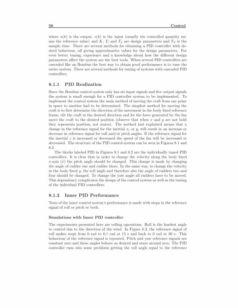
56 Control
where u(k) is the output, e(k) is the input (usually the controlled quantity mi-nus the reference value) and K, Ti and Td are design parameters and TS is thesample time. There are several methods for obtaining a PID controller with de-sired behaviour, all giving approximative values for the design parameters. Foreven better tuning, experience and a knowledge about how the different designparameters affect the system are the best tools. When several PID controllers arecascaded like on Bombus the best way to obtain good performance is to tune theentire system. There are several methods for tuning of systems with cascaded PIDcontrollers.
8.1.1 PID RealizationSince the Bombus control system only has six input signals and five output signalsthe system is small enough for a PID controller system to be implemented. Toimplement the control system the main method of moving the craft from one pointin space to another had to be determined. The simplest method for moving thecraft is to first determine the direction of the movement in the body fixed referenceframe, tilt the craft in the desired direction and let the force generated by the fanmove the craft to the desired position (observe that when x and y are not boldthey represents position, not states). The method just explained means that achange in the reference signal for the inertial xi or yi will result in an increase ordecrease in reference signal for roll and/or pitch angles. If the reference signal forthe inertial z is increased or decreased the speed of the fan will be increased ordecreased. The structure of the PID control system can be seen in Figures 8.1 and8.2.
The blocks labeled PID in Figures 8.1 and 8.2 are the individually tuned PIDcontrollers. It is clear that in order to change the velocity along the body fixedx-axis (x) the pitch angle should be changed. This change is made by changingthe angle of rudder one and rudder three. In the same way, to change the velocityin the body fixed y, the roll angle and therefore also the angle of rudders two andfour should be changed. To change the yaw angle all rudders have to be moved.This dependency complicates the design of the control system as well as the tuningof the individual PID controllers.
8.1.2 Inner PID PerformanceTests of the inner control system’s performance is made with steps in the referencesignal of roll or pitch or both.
Simulations with Inner PID controller
The experiments presented here are rolling operations. Roll is the hardest angleto control due to the direction of the wind. In Figure 8.3, the reference signal ofroll makes steps from 0 rad to 0.1 rad at 15 s and back to 0 rad at 30 s. Thisbehaviour of the reference signal is repeated. Pitch and yaw reference signals areconstant zero and these angles behave as desired and stays around zero. The PIDcontroller runs into some problems getting the roll angle equal to the reference
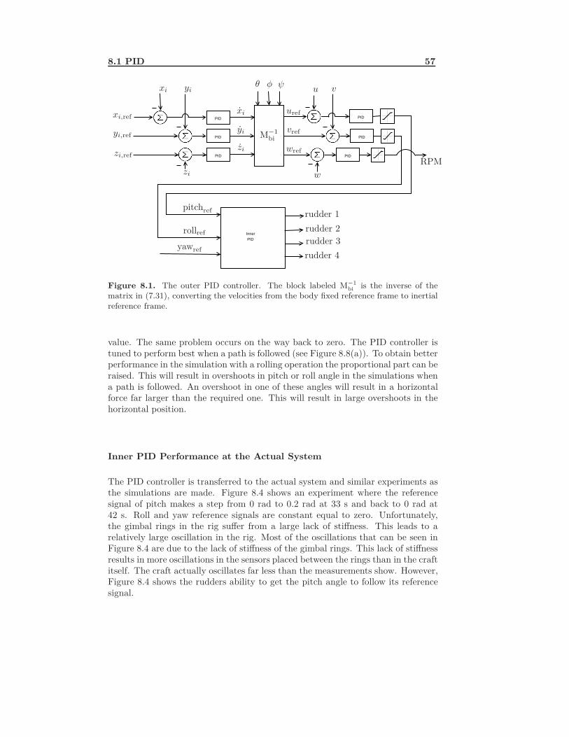
8.1 PID 57
PID
PID
PID
Inner PID
PID
PID
PID
xi,ref
yi,ref
zi,ref
xi yi
zi
xi
yi
zi
M−1bi
uref
vref
wref
u v
w
RPM
yawref
pitchref
rollref
rudder 1rudder 2rudder 3rudder 4
θ φ ψ
Figure 8.1. The outer PID controller. The block labeled M−1bi is the inverse of the
matrix in (7.31), converting the velocities from the body fixed reference frame to inertialreference frame.
value. The same problem occurs on the way back to zero. The PID controller istuned to perform best when a path is followed (see Figure 8.8(a)). To obtain betterperformance in the simulation with a rolling operation the proportional part can beraised. This will result in overshoots in pitch or roll angle in the simulations whena path is followed. An overshoot in one of these angles will result in a horizontalforce far larger than the required one. This will result in large overshoots in thehorizontal position.
Inner PID Performance at the Actual System
The PID controller is transferred to the actual system and similar experiments asthe simulations are made. Figure 8.4 shows an experiment where the referencesignal of pitch makes a step from 0 rad to 0.2 rad at 33 s and back to 0 rad at42 s. Roll and yaw reference signals are constant equal to zero. Unfortunately,the gimbal rings in the rig suffer from a large lack of stiffness. This leads to arelatively large oscillation in the rig. Most of the oscillations that can be seen inFigure 8.4 are due to the lack of stiffness of the gimbal rings. This lack of stiffnessresults in more oscillations in the sensors placed between the rings than in the craftitself. The craft actually oscillates far less than the measurements show. However,Figure 8.4 shows the rudders ability to get the pitch angle to follow its referencesignal.
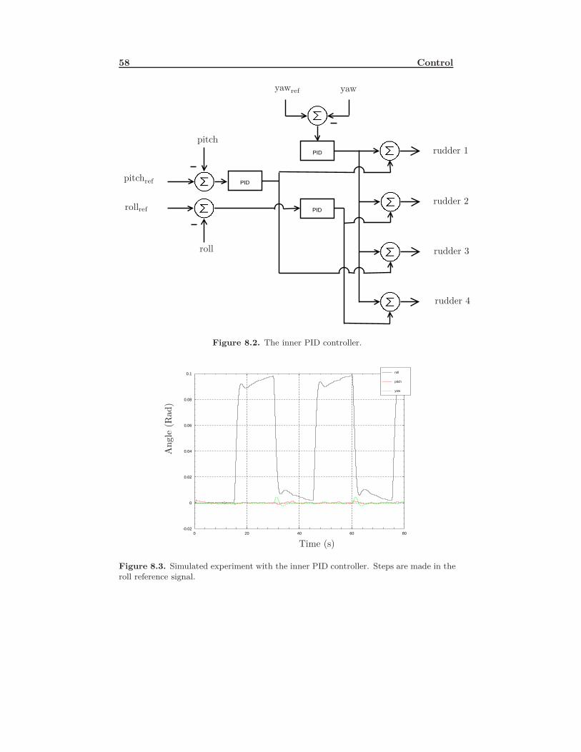
58 Control
PID
PID
PIDpitchref
rollref
yawref
pitch
roll
yaw
rudder 1
rudder 2
rudder 3
rudder 4
Figure 8.2. The inner PID controller.
6040200 80
0.08
0.06
0.04
0.02
0
-0.02
0.1 roll
pitch
yaw
Ang
le(R
ad)
Time (s)
Figure 8.3. Simulated experiment with the inner PID controller. Steps are made in theroll reference signal.
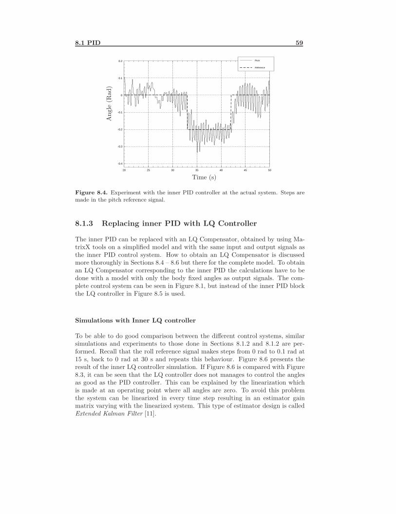
8.1 PID 59
454035302520 50
0.1
0
-0.1
-0.2
-0.3
-0.4
0.2 Pitch
Reference
Ang
le(R
ad)
Time (s)
Figure 8.4. Experiment with the inner PID controller at the actual system. Steps aremade in the pitch reference signal.
8.1.3 Replacing inner PID with LQ Controller
The inner PID can be replaced with an LQ Compensator, obtained by using Ma-trixX tools on a simplified model and with the same input and output signals asthe inner PID control system. How to obtain an LQ Compensator is discussedmore thoroughly in Sections 8.4 – 8.6 but there for the complete model. To obtainan LQ Compensator corresponding to the inner PID the calculations have to bedone with a model with only the body fixed angles as output signals. The com-plete control system can be seen in Figure 8.1, but instead of the inner PID blockthe LQ controller in Figure 8.5 is used.
Simulations with Inner LQ controller
To be able to do good comparison between the different control systems, similarsimulations and experiments to those done in Sections 8.1.2 and 8.1.2 are per-formed. Recall that the roll reference signal makes steps from 0 rad to 0.1 rad at15 s, back to 0 rad at 30 s and repeats this behaviour. Figure 8.6 presents theresult of the inner LQ controller simulation. If Figure 8.6 is compared with Figure8.3, it can be seen that the LQ controller does not manages to control the anglesas good as the PID controller. This can be explained by the linearization whichis made at an operating point where all angles are zero. To avoid this problemthe system can be linearized in every time step resulting in an estimator gainmatrix varying with the linearized system. This type of estimator design is calledExtended Kalman Filter [11].
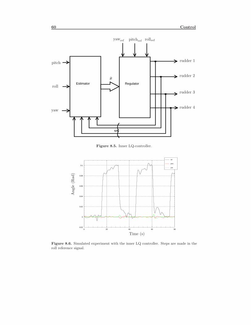
60 Control
Estimator Regulator
yaw
pitch
roll
yawref pitchref rollref
x
u
rudder 1
rudder 2
rudder 3
rudder 4
Figure 8.5. Inner LQ-controller.
6040200 80
0.08
0.06
0.04
0.02
0
-0.02
0.1
roll
pitch
yaw
Ang
le(R
ad)
Time (s)
Figure 8.6. Simulated experiment with the inner LQ controller. Steps are made in theroll reference signal.
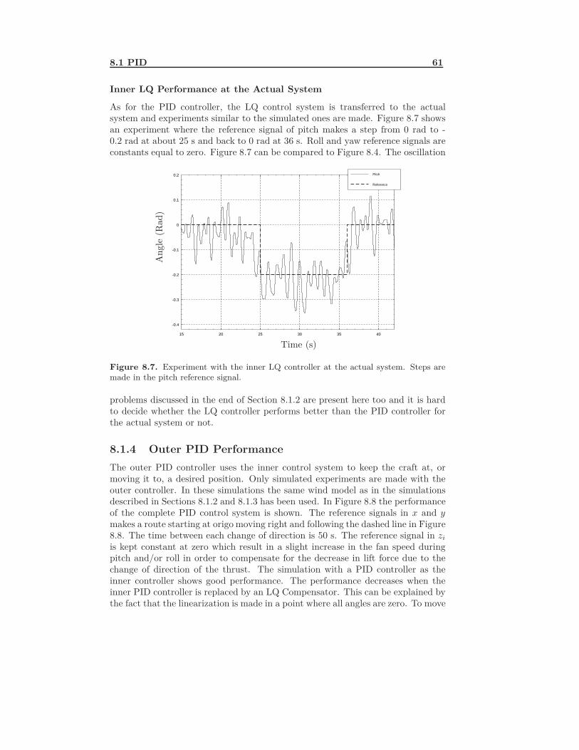
8.1 PID 61
Inner LQ Performance at the Actual System
As for the PID controller, the LQ control system is transferred to the actualsystem and experiments similar to the simulated ones are made. Figure 8.7 showsan experiment where the reference signal of pitch makes a step from 0 rad to -0.2 rad at about 25 s and back to 0 rad at 36 s. Roll and yaw reference signals areconstants equal to zero. Figure 8.7 can be compared to Figure 8.4. The oscillation
3530252015 40
0.1
0
-0.1
-0.2
-0.3
-0.4
0.2 Pitch
Reference
Ang
le(R
ad)
Time (s)
Figure 8.7. Experiment with the inner LQ controller at the actual system. Steps aremade in the pitch reference signal.
problems discussed in the end of Section 8.1.2 are present here too and it is hardto decide whether the LQ controller performs better than the PID controller forthe actual system or not.
8.1.4 Outer PID PerformanceThe outer PID controller uses the inner control system to keep the craft at, ormoving it to, a desired position. Only simulated experiments are made with theouter controller. In these simulations the same wind model as in the simulationsdescribed in Sections 8.1.2 and 8.1.3 has been used. In Figure 8.8 the performanceof the complete PID control system is shown. The reference signals in x and ymakes a route starting at origo moving right and following the dashed line in Figure8.8. The time between each change of direction is 50 s. The reference signal in ziis kept constant at zero which result in a slight increase in the fan speed duringpitch and/or roll in order to compensate for the decrease in lift force due to thechange of direction of the thrust. The simulation with a PID controller as theinner controller shows good performance. The performance decreases when theinner PID controller is replaced by an LQ Compensator. This can be explained bythe fact that the linearization is made in a point where all angles are zero. To move
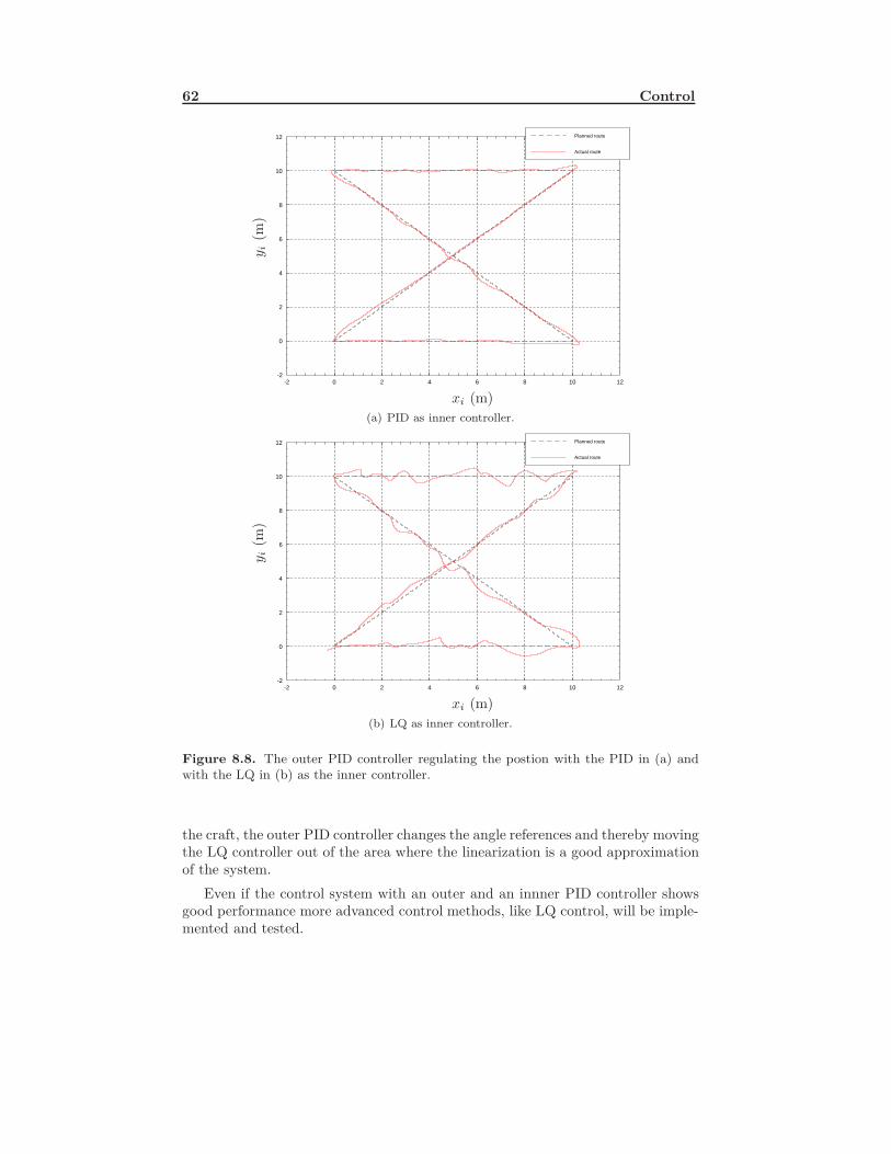
62 Control
1086420-2 12
10
8
6
4
2
0
-2
12 Planned route
Actual route
xi (m)
y i(m
)
(a) PID as inner controller.
1086420-2 12
10
8
6
4
2
0
-2
12 Planned route
Actual route
xi (m)
y i(m
)
(b) LQ as inner controller.
Figure 8.8. The outer PID controller regulating the postion with the PID in (a) andwith the LQ in (b) as the inner controller.
the craft, the outer PID controller changes the angle references and thereby movingthe LQ controller out of the area where the linearization is a good approximationof the system.
Even if the control system with an outer and an innner PID controller showsgood performance more advanced control methods, like LQ control, will be imple-mented and tested.
8.2 Linearization 63
8.1.5 Integral Windup for PID ControllerA single PID controller might suffer from integral windup if the control signal canbe saturated. The algorithm for introducing anti-windup for a discrete-time PIDcontroller, using conditional integration, is [4]
if not (control signal saturated) then In = In−1 + KTSTi
e(k) else In = In−1
u(k) = Ke(k) + In + KTdTS
(e(k) − e(k − 1)
)u(k) =
umax if u(k) > umax
u(k) if umin < u(k) < umax
umin if u(k) < umin
(8.2)
When several PID controllers are connected in cascade some information have tobe sent between them to prevent integral windup. If the inner subsystem’s controlsignal is saturated and the outer subsystem’s control signal is not, the incrementof the outer controller’s integrating part has to be stopped as well. If it is notstopped a similar effect as windup for a single PID controller can occur. The PIDcontrollers implemented on Bombus do not show any signs of integral windup.Therefore anti-windup is not implemented.
8.2 LinearizationEven if there exist control methods for nonlinear systems many modern controltools, like LQ control, require a linear model. Time-continuous nonlinear systemslike the model of Bombus are represented by the following differential and outputequations
x = f(x,u)y = g(x,u)
(8.3)
where x is the state vector, u is the input vector and y is the output vector. In thecomplete model of Bombus, the output vector contains all measurable magnitudes,position and body fixed angles of the craft. The input vector contains fan speedand angles of the four rudders. The states in the model are positions, velocities,angles and angular velocities of the craft, but also, for example, rudder angles.
If the nonlinearities have small affect on the system, the simplest way to lin-earize the system is to simply remove the nonlinear parts. In the Bombus modelthe nonlinearities affect the model too much for this method to be used. An-other way to linearize the model without removing the nonlinearities is to use thefirst-order term in the Taylor expansion. A Taylor expansion can be written as
f(x) = f(x0) +11!
f ′(x0)(x− x0) +12!
f ′′(x0)(x − x0)2 + . . .
· · · + 1n!
f (n)(x0)(x− x0)n +1
(n + 1)!f (n+1)(ζ)(x − x0)(n+1)
(8.4)
64 Control
where ζ is a point between x and x0. The firs-order part of (8.4) is the secondterm on the right side of the equality. Applying the first-order Taylor expansionto (8.3) results in
˙x = Ax + Bu + f0
y = Cx + Du(8.5)
where x = x − x0, u = u − u0, y = y − y0 and f0 = f(x0,u0) and
A =∂f(x,u)
∂x
∣∣∣x=x0,u=u0
B =∂f(x,u)
∂u
∣∣∣x=x0,u=u0
C =∂g(x,u)
∂x
∣∣∣x=x0,u=u0
D =∂g(x,u)
∂u
∣∣∣x=x0,u=u0
(8.6)
If (8.5) and (8.6) are applied to Bombus with x0 = 0 u0 = 0 and f0 = 0 thelinearized system becomes [
xy
]=
[A BC D
] [xu
](8.7)
where the matrices A, B, C and D are defined in (8.6) but with x0 = 0 andu0 = 0.
To be able to linearize the model, a simulation is done to put the system in acertain operating point represented by x0 and u0. At the selected operating pointthe fan runs at hovering speed and the rudders are all in initial position straightdown. The matrices A, B, C and D are obtained with the function lin afterrunning a simulation with the function sim in MatrixX SystemBuild. The lin-earization described above is described in the MatrixX manual as the linearizationused by the function lin.
8.3 DiscretizingThe linearized model obtained in the preceeding section is time-continous. How-ever, the control system is supposed to be implemeted in a computer and has tobe time-discrete. There are two different solutions to this problem.
One alternative is to create all necessary control tools from the continous sys-tem and, at last, discretize the complete control system. Doing this will involvean assumption that sample time, i.e., the time between two consecutive measure-ments from the sensors, is very small. An advantage of this alternative is thatthe discretizing is simple since there will be no derivatives in the complete controlsystem.
The other alternative is to discretize the system right after the linearizationand then create all control tools adapted to the discrete system. Using this methodremoves the assumption of very short time between measurements, but causes thediscretizing process to be harder. However, the discretizing can be done by usingthe tool discretize in MatrixX.

8.4 Estimator 65
The discrete system is expressed in state-space form as[xk+1
yk
]=
[A BC D
] [xk
uk
](8.8)
8.4 EstimatorTo be able to use state-feedback control all the states must be available. However,in real systems only the measurements are available and often corrupted by noise.An observer has to be constructed in order to get estimates of all the system states.Figure 8.9 illustrates the structure of the system with an observer. The following
ω
ν
u
x (Not measurable)
x (Estimated)
y (Measured)
Observer
Figure 8.9. Schematic figure of the actual system with an observer estimating the statevector.
equations describe the complete actual system:
x(t + 1) = Ax(t) + Bu(t) + Gω(t)y(t) = Cx(t) + ν(t)
(8.9)
where ω is the input noise with the noise gain matrix G. The measurement noiseis denoted ν. The intensity of the noise is described by[
Rωω Rων
RTων Rνν
]where Rωω represents the intensity of ω, Rνν represents the intensity of ν andRων represents the cross correlation between ω and ν. Rνν must be positivedefinite and Rωω = Rωω − RωνR
−1νν RT
ων must be positive semi-definite.The goal is to find an estimate of the states which minimizes the error between
the actual state vector, x, and the estimated state vector, x. The quadraticexpression to be minimized is
∞∑0
[xy
]T [Rωω Rων
RTων Rνν
] [xy
](8.10)
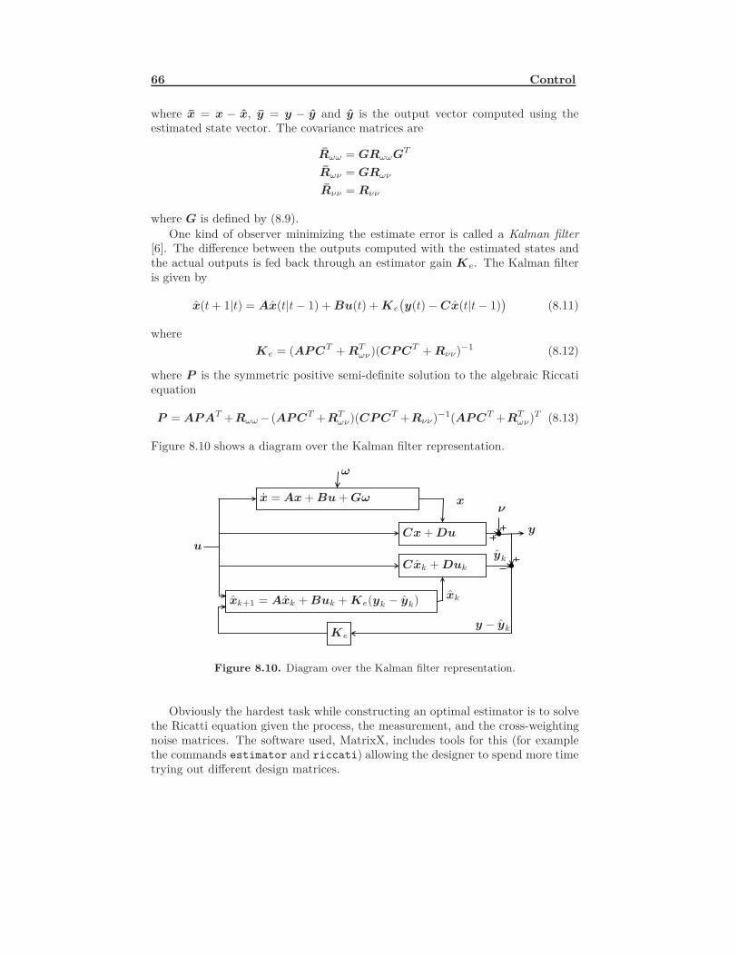
66 Control
where x = x − x, y = y − y and y is the output vector computed using theestimated state vector. The covariance matrices are
Rωω = GRωωGT
Rων = GRων
Rνν = Rνν
where G is defined by (8.9).One kind of observer minimizing the estimate error is called a Kalman filter
[6]. The difference between the outputs computed with the estimated states andthe actual outputs is fed back through an estimator gain Ke. The Kalman filteris given by
x(t + 1|t) = Ax(t|t− 1) + Bu(t) + Ke
(y(t) − Cx(t|t− 1)
)(8.11)
whereKe = (APCT + RT
ων)(CPCT + Rνν)−1 (8.12)
where P is the symmetric positive semi-definite solution to the algebraic Riccatiequation
P = APAT +Rωω− (APCT +RTων)(CPCT +Rνν)−1(APCT +RT
ων)T (8.13)
Figure 8.10 shows a diagram over the Kalman filter representation.
u
ω
x = Ax + Bu + Gω x
Cx + Du
xk+1 = Axk + Buk + Ke(yk − yk)xk
Cxk + Duk
yk
ν
y
y − ykKe
Figure 8.10. Diagram over the Kalman filter representation.
Obviously the hardest task while constructing an optimal estimator is to solvethe Ricatti equation given the process, the measurement, and the cross-weightingnoise matrices. The software used, MatrixX, includes tools for this (for examplethe commands estimator and riccati) allowing the designer to spend more timetrying out different design matrices.
8.5 Linear Quadratic Controller 67
8.5 Linear Quadratic ControllerThe Linear Quadratic Control System is a feedback controller with the goal tokeep the states within acceptable levels using acceptable amounts of control.
Using the system (8.9) an optimal feedback gain L minimizes the quadraticexpression [6]
∞∑0
[xu
]T [Qxx Qxu
QTxu Quu
] [xu
](8.14)
The matrix Qxx is real, symmetric and positive-semidefinite and is the weighting ofthe state vector elements. The matrix which determines the weight of the controlinputs is denoted Quu and is also real and symmetric, but positive-definite. Thematrix Qxu is the weight of the product of state vector elements and the controlinput elements. In many cases Qxu is set to zero, disregarding the products. In theBombus controller this matrix is set to zero. The expression (8.14) establishes thetrade-off between the permissible state fluctuation and amount of control requiredto move the states.
With Qxu = 0 the feedback law which minimizes (8.14) is
L = (BTSB + Quu)−1BTSA (8.15)
where S solves the Riccati equation
S = ATSA + Qxx − ATSB(BTSB + Quu)−1BTSA (8.16)
giving, together with the Kalman filter from Section 8.4, the optimal controller
x(t + 1) = Ax(t) + Bu(t) + Ke
(y(t) − Cx(t)
)u(t) = −Lx(t)
(8.17)
The controller explained above will steer the states to zero. This is not alwaysthe desired case on Bombus. Therefore a reference signal, r, has to be introduced.The system (8.9) can be extended with
z = Mx (8.18)
where z contains the states desired to control. The matrix M extracts the inter-esting states from x. This means that it is z − r that must be steered to zero.Introducing the reference signal in (8.17) gives
x(t + 1) = Ax(t) + Bu(t) + Ke
(y(t) − Cx(t)
)u(t) = −Lx(t) + Lrr(t)
(8.19)
The matrix Lr must be chosen so that the gain of the closed-loop system is equalto one [6] which in a discrete system in the static case means
M(I + BL − A)−1BLr = I (8.20)
If dim(z) = dim(u), Lr can be obtained by ordinary inversion. If dim(z) < dim(u)the reference gain can be obtained with the least-square method.
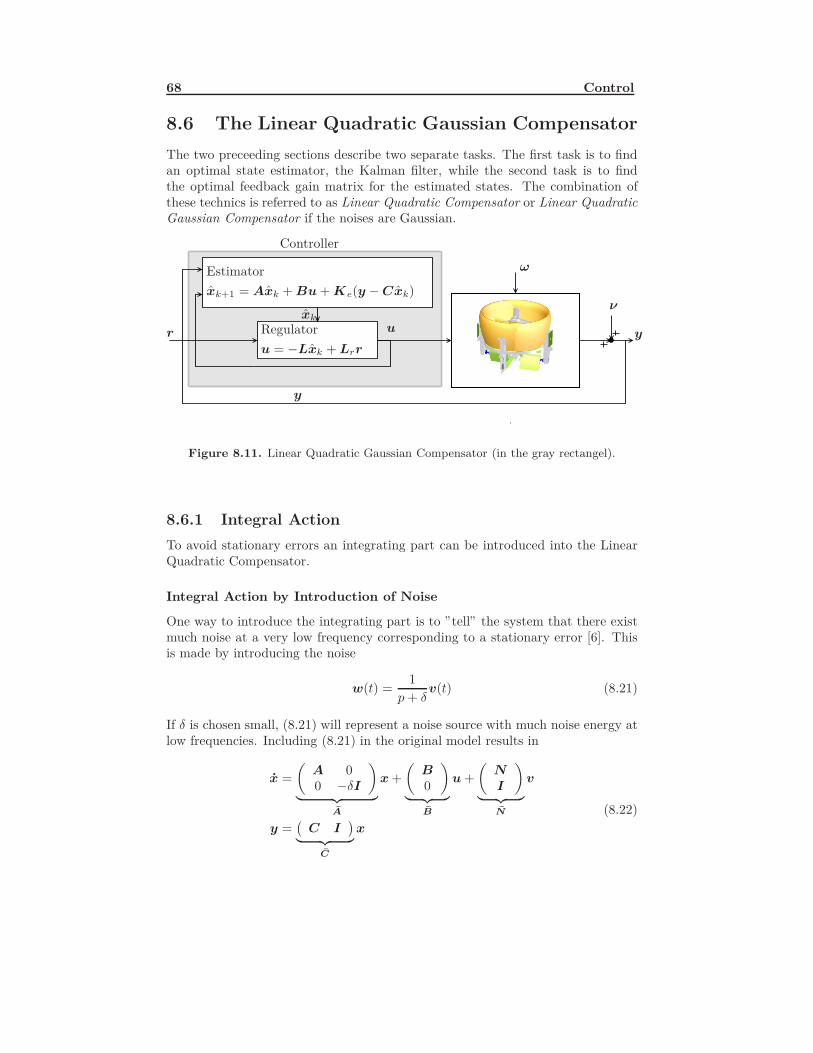
68 Control
8.6 The Linear Quadratic Gaussian CompensatorThe two preceeding sections describe two separate tasks. The first task is to findan optimal state estimator, the Kalman filter, while the second task is to findthe optimal feedback gain matrix for the estimated states. The combination ofthese technics is referred to as Linear Quadratic Compensator or Linear QuadraticGaussian Compensator if the noises are Gaussian.
u
ω
xk+1 = Axk + Bu + Ke(y − Cxk)
xk
u = −Lxk + Lrr
ν
y
y
r
Controller
Regulator
Estimator
Figure 8.11. Linear Quadratic Gaussian Compensator (in the gray rectangel).
8.6.1 Integral ActionTo avoid stationary errors an integrating part can be introduced into the LinearQuadratic Compensator.
Integral Action by Introduction of Noise
One way to introduce the integrating part is to ”tell” the system that there existmuch noise at a very low frequency corresponding to a stationary error [6]. Thisis made by introducing the noise
w(t) =1
p + δv(t) (8.21)
If δ is chosen small, (8.21) will represent a noise source with much noise energy atlow frequencies. Including (8.21) in the original model results in
x =(
A 00 −δI
)︸ ︷︷ ︸
A
x +(
B0
)︸ ︷︷ ︸
B
u +(
NI
)︸ ︷︷ ︸
N
v
y =(
C I)︸ ︷︷ ︸
C
x
(8.22)
8.6 The Linear Quadratic Gaussian Compensator 69
This requires that the system is discretized again (Section 8.3) and that a newLinear Quadratic Controller (Section 8.5)is computed using A, B, N and C. Thenew closed loop system will not have a stationary error.
Integral Action by Introducing extra States
Another way to introduce an integrating part into the system is to introduce statesrepresenting the errors. The additional states
xint = r − y = r − Cx (8.23)
can be introduced. Note that xint is a state vector with some dimension. Theadditional states inserted in the original system will result in the augmented system(
xxint
)=
(A 0
−C 0
)(x
xint
)+
(B0
)u +
(F0
)v +
(0I
)r (8.24)
If the original system is controllable and the systems transfer function is not zeroin the origin it can be shown that the augmented system (8.24) is also controllable[5]. The state feedback which in the original system was
u = −Lx
becomesu = −Lx − lintxint (8.25)
where lint should be chosen such that the closed loop system(x
xint
)=
(A − BL −Blint
−C 0
)(x
xint
)+
(F0
)v +
(0I
)r (8.26)
is asymptotically stable, meaning that the eigenvalues of(A − BL −Blint
−C 0
)should be inside the unit circle. With constant control input and reference signalthe system will converge to y = Cx, eliminating the stationary error.
Integral windup for Linear Quadratic Gaussian Compensator
Both methods for introducing integral action might suffer from integral windup.Integral windup occurs when the control signal is saturated and the reference valueof the state representing the saturated control signal is not fulfilled. This situationwill let the integrator in the controller grow which can result in large overshootsand slow return when the state has reached its reference value [1]. To solve thisproblem the increase of the integrating part must be stopped when the controlsignal is saturated. To stop the integrating part from increasing the condition
if ui < ui,min or ui > ui,max
then xi(k + 1) = xi(k)else xi(k + 1) = Aix + Biu
70 Control
where Ai and Bi is the part of the A and B matrices affecting xi, can be used.In the experiments and simulations made on Bombus no integral windup has beendetected. Becasue of this and lack of time, the solution to the problem explainedabove will not be implemented.
8.6.2 LQ RealizationThe complete time-continous model is linearized at a hovering operating pointusing the tools available in MatrixX and SystemBuild. Before the linearization,the input signals are balanced. This means that the fan speed control signal isresized to about the size of the rudder control signals. The linearization gives astatespace system with 19 states, three of them uncontrollable.
Selecting Suitable Weighting Matrices
The estimator matrix Rωω and Rνν are tuned to describe the noise well and givegood estimates of the states. The cross-weighting matrix Rων is set to zero.
The weighting matrix Qxx will only contain zeros except for the diagonal el-ements. Every element in the diagonal of the matrix describes the cost of oneparticular state variable. To create the Linear Quadratic Compensator it is notnecessary that all states are controllable but the system must be stablizable. Theuncontrollable states have to be taken under special consideration when the weight-ing matrices are chosen.
The weighting matrix Quu will also be a diagonal matrix. Since the controlvariables from the controller are the signals to the four rudders all the elementswill be equal. The values of the elements are trimmed to give good performance.
Introducing an Integrating Part
To remove possible stationary errors an integrating part is added to the model.The solution used is the method of adding low frequency noise to certain statesdescribed in the first part of Section 8.6.1. Before the introduction a stationaryerror was present in several states but it was in the z-state where it was mostobvious. The introduction of the low frequency noise completely removed thisstationary error.
Creating the Observer and the Controller
After selecting the weighting matrices the observer and the controller are obtainedwith the commands estimator and regulator in MatrixX. The feedback gainmatrix Kr is obtained and the reference gain matrix Lr is calculated using (8.20).
8.6.3 LQ PerformanceThe simulated performance of the LQ-controller can be seen in Figure 8.12. Inthe simulation a reference flight path like the one used to test the PID controlleris used (see Section 8.1.2), represented by the dashed line. The flight path of the

8.6 The Linear Quadratic Gaussian Compensator 71
craft is the solid line. As noise a wind as described in Section 6 is used. This meansthat the wind speed is white Gaussian noise with a mean value and the angle fromwhich the wind arrives varies from +π
6 rad to −π6 rad. When the wind arrives
from 0 rad it is arriving from negative xi. The performance of the LQ-controlleris acceptable with a position error of at most 0.5 m.
1086420-2 12
10
8
6
4
2
0
-2
12
Planned route
Actual route
xi (m)
y i(m
)
Figure 8.12. The Linear Quadratic Compensator performance.
The kind of surveillance for which Bombus is primarily designed only requiresthe craft to hold one position. Therefore, simulations were made to determine thecontrol systems ability to hold the craft at one point in space. The result canbe seen in Figure 8.13. The wind is the same as in the simulations above. It isclear that the control system is unable to keep the craft completely motionless butthe performance of the control system is satisfactory since the maximum positionerror is no larger than the diameter of the craft. The reference value for zi is alsokept to zero resulting in Figure 8.14.
To explain the fact that the control system is unable to keep the craft at thedesired position the estimations from the observer can be studied. Even if all statesare available in the simulations only the states available in the physical system areused. To analyse the Linear Quadratic Compensator the estimated states can becompared to the actual states available in the simulations. The difference betweensome of the estimated states and the corresponding actual states for the simulationwith a constant reference signal equal to zero can be seen in Figure 8.15. The figureshows that the measured states x and y are well estimated. However, z, roll, pitchand yaw are measured as well, but are not estimated as good as x and y. Theexplaination is that the rudders are positioned slightly off from the initial positionto counteract the wind. In the model used for computing the Estimator the windis not included more than as a Gaussian noise. The Estimator estimates the states

72 Control
0.20.10-0.1-0.2-0.3 0.3
0.2
0.1
0
-0.1
-0.2
-0.3
0.3
xi (m)
y i(m
)
Figure 8.13. Performance of the Linear Quadratic Compensator when reference signalsare constants equal to zero.
806040200 100
0.3
0.25
0.2
0.15
0.1
0.05
0
-0.05
0.35
z i(m
)
time (s)
Figure 8.14. Performance along the z-axis of the Linear Quadratic Compensator whenreference signals are constants equal to zero.
at the next time point knowing only the present value of the states and the signalssent to the rudders and the fan. These estimations will differ from the actualstates since the actual states will also be affected by the mean value wind. TheEstimator minimizes the variance of the estimation error.

8.7 Other Controllers 73
0.2
0
-0.2
-0.4
0.4
0.2
0
-0.2
-0.4
0.4
0.2
0
-0.2
-0.4
0.4
0.2
0
-0.2
-0.4
0.4
0.2
0
-0.2
-0.4
0.4
0.2
0
-0.2
-0.4
0.4
0.2
0
-0.2
-0.4
0.4
0.2
0
-0.2
-0.4
0.4
0.2
0
-0.2
-0.4
0.4
0.2
0
-0.2
-0.4
0.4
0.2
0
-0.2
-0.4
0.4
0.2
0
-0.2
-0.4
0.4
x− x y − y z − z
roll− ˆroll pitch− ˆpitch yaw− ˆyaw
p− p q − qr − r
u− u v − vw − w
Figure 8.15. Estimation errors of interesting states.
8.7 Other ControllersThe above mentioned controllers have been implemented, simulated and some ofthem have been tested on the physical system. The potential performance of somealternative controllers have been discussed. These controllers have because of lackof time never been implemented and their performance have therefore not beencompared to the performance of the previously discussed controllers.
8.7.1 Model Predictive ControlModel predictive control, MPC, is a modern control method that uses knowledgeof the future state of the system to calculate an optimal control law. MPC hasonly been available in commercial applications for about 20 years [4]. This isdue to the fact that MPC requires a large number of calculations each sampleand the computers have not been fast enough until recently. Over the last fewyears, computers have become fast enough to implement MPC in systems evenwith very fast dynamics. In very slow systems, like for example the processes inan oil refinery, MPC has been used for quite some time.
MPC has several advantages compared to LQ-control. The main advantage isMPC’s ability to handle constraints on the output signals. The LQ-control sys-
74 Control
tem can have limited signals but the control system will not take this limitationsunder consideration. The MPC control system, on the other hand, will take thelimitations under consideration and compute an optimal control law. The maindisadvantage of MPC compared to LQ is that MPC require more online calcula-tions.
MPC Method
The MPC algorithm is [1]
1. Measure/estimate the current states.
2. Calculate a control sequence using the optimization described below.
3. Apply the first element of the control sequence to the system.
4. Time update (k = k + 1).
5. Go to step one.
The procedure to calculate the control sequence will now be described. A discretemodel can be written as
x(k + 1) = Ax(k) + Bu(k)y(k) = Cx(k)
(8.27)
where x, y, and u can be vectors if the system is multidimensional. As the nameof the method implicates a prediction of the future has to be made. A predictionof the future system is calculated as
x(k + 2) = Ax(k + 1) + Bu(k + 1)
= A2x(k) + ABu(k) + Bu(k + 1)(8.28)
These equations can be written as
X = Hx(k) + SU
where
X =
x(k + 1)x(k + 2)
...x(k + MMPC)
H =
AA2
...AMMPC
U =
u(k)u(k + 1)
...u(k + MMPC − 1)
8.7 Other Controllers 75
S =
B 0 · · · 0AB B · · · 0...
.... . .
...AMMPC−1B AMMPC−2B · · · B
For MPC to be effective the model has to have a prediction horizon. Theprediction horizon is the number of time samples into the future the states arepredicted. The choice of prediction horizon is important to get the desired be-haviour of the control system and should be made so that the horizon covers anordinary settling [1]. If the prediction horizon is chosen to short the controller willnot be able to predict the entire settling and thereby not include enough of themodel dynamics in the computations to be able to obtain a good enough controllaw. On the other hand, if the prediction horizon is chosen too large, the numberof calculations needed will be large. The prediction horizon is denoted MMPC.The control horizon, denoted NMPC, is often MMPC − 1 but if it is possible, anas small as possible NMPC is desired since this would lessen the complexity of thecalculations.
The function
∞∑j=0
||x(k + j + 1)||2Q1+ ||u(k + j)||2Q2
(8.29)
is the function minimized in a LQ-controller. Replacing ∞ with the predictionhorizon minus one will give the function to minimize in MPC. Introducing thematrices
Q1 =
Q1
Q1
. . .Q1
, Q2 =
Q2
Q2
. . .Q2
The matrices Q1 and Q2 are design parameters or weight matrices indicating theimportance of the different x and u.
If the prediction horizon is inserted in (8.29) it can be rewritten as
MMPC−1∑j=0
||x(k + j + 1)||2Q1+ ||u(k + j)||2Q2
= XT Q1X + UT Q2U
= (Hx(k) + SU)T Q1(Hx(k) + SU) + UT Q2U
(8.30)

76 Control
Introducing a reference signal, r, in (8.30) givesMMPC−1∑
j=0
||y(k + j + 1) − r(k + j + 1)||2Q1+ ||u(k + j)||2Q2
=
=(C(Hx(k) + SU) − R
)TQ1
(C(Hx(k) + SU) − R
)+ UT Q2U =
= (CHx + CSU − R)T Q1(CHx + CSU − R) + UT Q2U =
= (CHx− R)T Q1(CHx− R) + 2(CHx − R)T Q1CSU+
+ UTST CTQ1CSU + UT Q2U
(8.31)
where
C =
CC
. . .C
and R =
r(k + 1)r(k + 2)
...r(k + MMPC)
and C is the matrix from (8.27).A standard Quadratic Programming, or QP, problem can be written as
minx
12xTHx + fTx
subject to Ax ≤ b(8.32)
The expression (8.31) can be rewritten to fit the form of (8.32) by removing termsnot depending on U and dividing by two.
minU
12UT (ST C
TQ1CS + Q2)U +
(Q
T
1 CTST (CHx − R)
)U
subject to U ≤ U limit
(8.33)
If the constraints are
−yi,max ≤ yi ≤ yi,max i = 1, 2, . . . ,n (8.34)
the constraints for the entire system can easily be expressed. Since Y = C(Hx(k)+SU) according to (8.28) and (8.30) the constraints in (8.34) can be written as[
I−I
]C(Hx(k) + SU) ≤
[Y maxY max
]⇒[
I−I
]CSU ≤
[Y maxY max
]−
[I−I
]CHx(k) ⇒
AyU ≤ by
(8.35)
This will give the optimization
minU
12UT
(ST C
TQ1CS + Q2
)U +
(Q
T
1 CTST (CHx− R)
)U
subject to AyU ≤ by
(8.36)
8.7 Other Controllers 77
MPC for Bombus
The Bombus model consists of nineteen states. Apart from the nine states inSection 7.4 the roll, pitch and yaw angles and the rudder angles are also used asstates. The model is nonlinear and since only linear MPC will be investigated alinearization (se Section 8.2) has to be made. Denote the linearized discrete model
x(k + 1) = ALx(k) + BLu(k)y(k) = CLx(k)
(8.37)
The matrices in the linearized discrete model above can be computed using Ma-trixX. The optimization problem will look like (8.36), but with AL, BL and CLinstead of A, B and C.
There are no physical constraints on the output signals for Bombus. Since themodel is linearized, constraints can be put on the signals to limit the movement ofthe craft in order to keep it within an area where the linearized model is acceptable.The pitch and roll angles, for example, can be restrained to − π
18 ≤ roll ≤ π18 . If
only the restraints on roll and pitch are considered the matrix [I, − I]T in (8.35)must be modified so that all terms except those multiplied with roll and pitch arezero.
The MPC-controller puts high demands on the calculation capability of thecomputer since the QP-problem (8.36) has to be solved in every time sample. Itis possible that the processor used on Bumbus does not have the required cal-culation capacity. With a new faster processor installed it is not unlikely thatthe MPC-controller will perform better than the LQ and PID controllers in manyways. Another solution to the problem with the lack of computational capability isExplicit MPC or EMPC. EMPC performs some of the required calculations offlinereducing the number of calculations needed to be performed online [3]. EMPCwill not be further investigated in this report.
8.7.2 BacksteppingIn the late 1980’s a new method for nonlinear control was introduced. The methodis based in on the Lyapunov theory and it is called backstepping. As the namesuggests backstepping uses a recursive algorithm to obtain a control law as well asa proof of stability. The recursive algorithm gives a systematic way of calculatinga Lyapunov function used to determine this stability. Unlike most other controlmethods for nonlinear systems, backstepping does not necessary try to removeor linearize nonlinearities. Instead, backstepping uses the stabilizing propertiesof the nonlinearities to obtain a control law that might require less control effortcompared to a method linearizing the nonlinearities.
Lyapunov Theory
Lyapunov functions are used to determine stability for nonlinear systems by exam-ining the distance between x and a stable equilibrium x0. First we must consider
78 Control
a system x = f(x). A function
W (x0) = 0 W (x) > 0, x = x0 Wx(x)f(x) ≤ 0 (8.38)
where Wx = (∂W/∂x1, . . . , ∂W/∂xn) can be interpreted as the distance between xand x0, is called a local Lyapunov function. If the Lyapunov function also satisfies
W = Wxf(x) < 0, x = x0 and W (x) → ∞, |x| → ∞ (8.39)
the point x = x0 is said to be a globally asymptotically stable equilibrium [6, 9].If a new nonlinear system
x = f(x,u) (8.40)
is considered, a control lawu = k(x) (8.41)
can be constructed for the system. To determine whether the control law is a glob-ally stabilizing control law, a Lyapunov function for the system using that controllaw can be constructed. This Lyapunov function is called a control Lyapunovfunction, or a clf. A Lyapunov function satisfying (8.38) and
infu
Wxf(x,u) < 0, x = 0 (8.42)
is a clf [9]. If a clf can be constructed the control law is globally stabilizing and ifthe control law is globally stabilizing a clf can always be constructed.
Control using Backstepping
The Lyapunov control described above requires that the clf is known. Belowbackstepping as described in [9] will be used to obtain a control law and a clf.Consider the system
x = f(x, ξ)
ξ = u(8.43)
where x and ξ are state variables and u is the control input. A virtual control lawcan be constructed
ξ = ξdes(x) (8.44)
making x = 0 a globally asymptotically stable equilibrium. The stability can beshown with a clf, W1(x). The clf should be choosen such that (8.43) and (8.44)satisfies
W1|ξ=ξdes = W1,x(x)f(x, ξdes) < 0, x = 0 (8.45)
A residual can be constructed as
ξ = ξ − ξdes(x) (8.46)
8.7 Other Controllers 79
and the control input u can be used to steer ξ to zero which in turn results in thedesired ξ = ξdes. If (8.46) is inserted into the system (8.43) the result is
x = f(x, ξ + ξdes) f(x, ξdes(x)
)+ Ψ(x, ξ)ξ
˙ξ = u − ∂ξdes
∂x(x)f
(x, ξ + ξdes(x)
) (8.47)
where f(x, ξdes) is the desired dynamics of the system and
Ψ(x, ξ) =f(x, ξ + ξdes(x)) − f(x, ξdes)
ξ
For the augmented system (8.47) a new clf can be obtained using W1(x) andweighting ξ. In [9]
W2(x, ξ) = W1(x) +12ξ2
(8.48)
is used. According to (8.39), W2 must satisfy W2 < 0 for the control law to be aglobally stabilizing control law. Differentiating (8.48) with help from (8.47) gives
W2 = W1,x(x)[f(x, ξ + ξdes) + Ψ(x, ξ)ξ
]+ξ
[u − ∂ξdes
∂x(x)f
(x, ξ + ξdes(x)
)]=
= W1,x(x)f(x, ξdes(x)
)+ ξ
[Wx(x)Ψ(x, ξ) + u − ∂ξdes
∂x(x)f
(x, ξ + ξdes(x)
)](8.49)
The term W1,x(x)f(x, ξdes(x)) in (8.49) is according to (8.45) negative if x = 0.To satisfy (8.39), u in (8.49) has to be carefully chosen. By selecting
u = −W1,x(x)Ψ(x, ξ) +∂ξdes
∂x(x)f(x, ξ + ξdes(x)) − ξ (8.50)
all terms inside the last brackets in (8.49) will be cancelled out except −ξ. Thisresults in
W2 = W1,x(x)f(x, ξdes) − ξ2< 0, x = 0, ξ = 0 (8.51)
Now both a globally stabillizing control law, u, and a Lyapunov function, W2, hasbeen calculated and can be used for control of the nonlinear system.
Backstepping applied to Bombus
Backstepping for rigid bodies as explained in [9] can easily be applied to theBombus model. The first six equations in (7.30) in Section 7.4 can be rewrittento fit the form presented in [9]. Then the model can be written as
V c = −ω × V c +1m
F
Iω = −ω × Iω + T(8.52)

80 Control
where V c is the velocity vector, ω is the angular velocity vector, T is the torquevector, F is the force vector and I is a matrix containing the moment of inertiaabout the three axes. This means that
V c =
u
vw
ω =
p
qr
I =
Ix 0 0
0 Iy 00 0 Iz
T =
L
MN
(8.53)
To perform the backstepping procedure F has to be divided into two parts
F = m(F aero(V c) + uV V c
)(8.54)
where
F aero =
X
YZ
, V c =
1|V c|V c (8.55)
and uV is a control parameter. The last part of (8.54) is an approximation ofthe thrust of an engine in the direction of V c. For simplicity the effect of gravityhas been included in X Y and Z in F aero. If (8.52) – (8.55) are combined, theequations in Section 7.4 are obtained.
To perform the backstepping algorithm for the rigid body a steady state, de-scribed by V 0 and ω0, is required. In the Bombus case, the trivial steady stateV 0 = (0 0 0)T and ω0 = (0 0 0)T is the the one best suited. To start the back-stepping algorithm the second equation in (8.52) can be rewritten as
ω = I−1(T − ω × Iω) = uT (8.56)
resulting, together with (8.52) and (8.54), in
V c = −ω × V c + F aero(V c) + uV V c
ω = uT (8.57)
In [9], a virtual control law ω = ωdes is introduced together with the Lyapunovfunction
W1 =12(V c − V 0)T (V c − V 0) (8.58)
Combining the suggested Lyapunov function, the suggested virtual control lawand (8.57) gives
W 1 = (V c − V 0)T(− ωdes × V c + F aero(V c) + uV V c
)(8.59)
To cancel out F aero(V c) and to achieve W ≤ 0 the choices
uV = k1(V 0 − V c)T V c − VT
c F aero(V c)
8.7 Other Controllers 81
ωdes = k2(V 0 × V c) +1
|V c| V c × F aero(V c) (8.60)
are logical, giving
W 1 = −k1
((V 0 − V c
)TV c)2 − k2|V 0 × V c|2 −U(V c,V 0) ≤ 0 (8.61)
The next step in the backstepping method is to construct the residual
ξ = ω − ωdes
Inserting the above residual in the system (8.57) results in
V c = −ωdes × V c + F aero(V c) + uvV − ξ × V c
ξ = uT + Φ(V c, ξ)(8.62)
whereΦ(V c, ξ) =
d
dtωdes
In the first equation of (8.62) only the last cross product is not a part of thedesired dynamics of the system. Like in (8.48) the existing Lyapunov functionnow has to be extended to
W 2 = k3W 1 +12ξT ξ
giving the derivative
W 2 =
= k3(V c − V 0)T(− ωdes × V c + F aero(V c) + uV V − ξ × V c
)+ ξT
(uT − Φ(V c, ξ)
) (8.63)
If the control lawuT = k3(V 0 × V c) − k4ξ + Φ(V c, ξ)
is used (8.63) becomes
W 2 = −k3U(V c,V 0) − k4ξT ξ ≤ 0
where U(V c,V 0) is defined in (8.61). The last equality in (8.63) is calculatedthrough major simplifications. These simplifications and the complete calculationsfrom the section above can be seen in [9]. The control laws now calculated togetherwith the Lyapunov function makes the system converge to V c = V 0 and ξ = 0.
Backstepping is well suited for use in airplane control and can also seem to bewell suited for Bombus. When calculating the backstepping equations for Bombusone realize soon that the first equation in (8.60) will cause a singularity as themagnitude of the velocity |V c| approaches the desired steady state V 0 = (0 0 0)T .This problem has to be solved before backstepping can be used on Bombus.
82 Control
8.8 Comparing Controller PerformanceFrom the discussions about the performance of the different control systems it iseasy to see a clear difference. The inner PID/outer PID control system performsgood with a position error of only a few decimeters while the inner LQ/outer PIDcontrol systems perform poorly with a position error of sometimes almost onemeter. The LQ Compensator performs satisfactory with a position error of lessthan one meter.
8.8.1 Reasons for Choosing the LQ ControllerBoth the MPC and backstepping controllers have the potential to give a goodperformance for Bombus. Both controllers also have disadvantages in their use onBombus compared to LQ and PID. The main reason for choosing the LQ and PIDcontrollers instead of the other controllers is the simplicity to implement them.Several commands exist in MatrixX simplifying the implementation of both anLQ and a PID controller. Simplicity was preferred to possible better performanceboth because of the limited time available and because of the wishes from DSTControl AB.
Chapter 9
Results
The goals of this thesis were to examine the performance of a ducted fan UAVregarding lift capacity, position accuracy and wind tolerance. The performancewas to be tested with help of a control system that had to be constructed andimplemented. A mathematical model should be constructed to facilitate the designof the control system. This chapter will discuss whether the goals are achieved ornot.
9.1 ConclusionsThe overall conclusion is that the goals are achieved. A mathematical model hasbeen developed and used to design two different control systems. The model isverified with different experiments, for example lift force experiments, which alsogave an opinion on the lift force performance. Simulations are made with the twocontrol systems at the model to examine position accurancy and wind tolerance.
9.1.1 Discussion regarding Lift ForceLift force experiments have been made while designing the mathematical model.The conclusion regarding lift force is that the craft needs more lift force to be ableto lift cables, mission equipment and its own mass. Chapter 4 gives a detailedinvestigation of the lift force.
9.1.2 Discussion regarding the ModelThe mathematical model has been developed using physical modeling. Most ofthe physical relations used in the model are either trivial or has been verified inexperiments with the prototype in a test rig. The test rig has been developedduring this thesis as well. We believe that the mathematical model describes theducted fan UAV good at free flight, but not as good in the test rig. No frictionor moment of inertia of the test rig has been modeled. However the test rig has
83
84 Results
been very useful in getting an understandig of the UAV’s performance. Chapter7 gives a detailed description of the mathematical model.
9.1.3 Discussion regarding the Control Systems
Two different control systems have been designed. One of them is constructed asa cascade of two control systems, outer and inner. The other control system usesLinear Quadratic control tools.
Cascaded Controllers
One of the control systems uses straight forward PID methods. In this case twoof the rudders are controlled by a PID regulator controlling roll, the other tworudders are controlled by another PID regulator controlling pitch. The signalsfrom the two mentioned PID regulators are added together with the signal from athird PID regulator controlling yaw rotation. This control system manages to bothkeep the system stable and follow a reference signal with satisfactory performance.
An additional PID controller is designed to control the reference signals inroll, pitch and yaw. In this way the position can be controlled. For example anegative pitch angle change the direction of the force generated by the propellerand a composant in positive x direction occurs. In a similar way roll can be usedto regulate the position in y. When the force generated by the propeller gets ahorizontal composant the lift force is reduced. Another PID regulator is designedto regulate the position in z by varying the fan speed. This means the fan speedis increased during horizontal movement to keep the craft from descending. Thissystem of PID regulators is refered to as the outer PID controller.
The cascade system of the outer and the inner PID controllers has been testedin simulations with a good result which can be seen in Section 8.1.4.
An alternative control system for controlling roll, pitch and yaw is designedusing Linear Quadtratic control tools. The performance of this control system isworse than the PID control system especially when a reference singnal is followed.The worse performance is explained by the fact that the constant estimator matrixis chosen based on a linearization made at operating point with all angles zero.At larger angles the linearization is not as concordant with the model as for smallangles. This means that the LQ controller is good at keeping the craft stable butsince movement is achieved by pitching or rolling the craft the controller performesworse when a reference signal is followed. The result of a simulated flight can beseen in Section 8.1.4.
Unfortunally the test rig is in a rather bad shape which generates some prob-lems validating the control systems at the actual system. However, disregardingthe problems caused by the test rig, experiments show that the actual system fol-lows a reference signal at roll or pitch quite good. Only the inner control systemscan be tested at the actual system, since there are no sensors measuring posi-tion and the test rig is constructed to keep the craft fixed in space, only allowingrotations.
9.2 Summary 85
Linear Quadratic Compensator
The other control system is designed using tools from MatrixX to generate an es-timator and a regulator. This control system takes only the three inertial positioncoordinates as reference and tries to keep the rest of the states to zero. This meansthat this control system only can be tested in simulations. This has been donewith quite good results. Simulated experiments with varying reference positionshas shown good performance.
Chapter 8 gives a detailed descripition of the outer and inner control systemsand also discusses alternatives.
9.1.4 Discussion regarding Wind ToleranceThe wind tolerance has not been tested in experiments at the actual system. Amodel of the wind has been implemented in the mathematical model and in thesimulated experiments a slight wind has been included.
It has been shown that the systems original configuration was not able tocompensate for any wind at all. To get the ability to keep the system stableeven with a wind disturbance, the forces from the rudders had to be increasedwithout increasing their wind exposure. The actual system has been equippedwith twin rudders to make the rudder area exposed for the wind induced by thepropeller (vertical) larger but leaving the rudder area exposed for the disturbancewind (horizontal) the same. This modification of the UAV was implemented in themodel as well and the ability to compensate for disturbance wind was increased.
The size of the wind used in the simulated experiment is still not as large asdesired and raising it makes the system unstable. There is no solution to thisproblem with the current configuration. Increasing all dimensions in a futureprototype would probably also increase the wind tolerance as well as the lift force.
Chapter 6 more deeply discusses wind and other noises affecting the UAV.
9.2 SummaryThe goals of the thesis are achieved with varying, mostly positive, results. Acontinued development of the concept will be considerable facilitated by the guidelines given by this report.

86 Results
Chapter 10
Future work
If DST Control AB decides to continue the development of the ducted fan UAVthere are several different areas where improvements can be made.
10.1 The CraftThe current prototype is sufficient for the experiments conducted in this projectbut if more advanced testing, like free flight tests, shall be made the constructionof a new prototype is recommended. The design of the new prototype ought to bedeveloped with a more solid theoretical ground than the current prototype. Theduct can be constructed in a way that increases the lift without sacrificing any ofthe benefits of the current duct.
Both the propeller and the rudders on the current prototype are far fromoptimal. A theoretical study could result in a propeller with the ability to generatelarger lift without a larger radius and rudders with the ability to generate largerforce without a larger area.
10.2 SensorsNew sensors for the prototype is essential for more advanced experiments with amore advanced test rig or in free flight. Most of the sensors currently used have alow resolution and are very sensitive to noise. The pitch and roll sensors are lowprice rotational potentiometers placed on the test rig in a way that decreasesthe accuracy further. A set of sensors consisting of high precision gyros andaccelerometers are intended for the final product. These sensors would give bettermeasurements but require some calculations to measure the correct angles.
10.3 Test RigTest Rig Beta was built with a minimal budget resulting in a test rig constructedby inferior materials and with poor size precision. This has resulted in a gimbal
87
88 Future work
with far to flexible rings and axles which are not centered. The flexibility of the righas affected the experimental results in a negative way which can clearly be seenon the extensive oscillations of the angles in Section 8.1.3. A new test rig withstiffer gimbal rings made of light weight metal could improve the experimentalresults considerably.
Another option is to construct a completely different test rig. Some suggestionsfor alternative test rig are given in Chapter 3.
10.4 ControllerEven though two of the resulting controllers implemented in this project per-form satisfactory in most cases, better controllers can, without too much effort,be implemented. Another model based controller, like EMPC or backsteppingdiscussed earlier, might perform better than both the LQ and PID controllers.The controller structure might also be improvable to achieve a simpler and moreeffective structure.
Modifications can be made to the existing controllers to achieve better perfor-mance. The current LQ control system uses only a single linearization. Using anExtended Kalman Filter to linearize in every time sample would improve the per-formance of the controller but it would require more calculation capacity from theprocessor. The currently used processor might not have the required calculationcapacity and would have to be replaced by a more powerful processor.
Bibliography
[1] Daniel Axehill and Johan Sjöberg. Adaptive Cruise Control for Heavy Vehi-cles. Hybrid Control and MPC. 2003. Department of electrical engineering,Linköping University.
[2] Henry Choi, Peter Sturdza, and Richard M. Murry. Design and constructionof a small ducted fan engine for nonlinear control experiments. In AmericanControl Conference, 1994. Department of Mechanical Engineering, CaliforniaInstitute of Technology, June 1994.
[3] Mats Ekström. Slutfasstyrning av missil med explicit prediktionsreglering.2005. Department of electrical engineering, Linköping University.
[4] Torkel Glad, Svante Gunnarsson, Lennart Ljung, Tomas McKelvey, AndersStenman, and Johan Löfberg. Digital Styrning. Kurskompendium. 2003.Department of electrical engineering, Linköping University.
[5] Torkel Glad and Lennart Ljung. Reglerteknik. Grundläggande teori. Stu-dentlitteratur, 1989. ISBN 91-44-17892-1.
[6] Torkel Glad and Lennart Ljung. Reglerteori. Flervariabla och olinjärametoder. Studentlitteratur, 2003. ISBN 91-44-03003-7.
[7] NASA Great Images in NASA. Full description of image c1960-53088. URL:http://grin.hq.nasa.gov/ABSTRACTS/GPN-2000-000379.html, September16 2005.
[8] John Hauser and Ali Jadbabaie. Aggressive maneuvering of a thrust vectoredflying wing: A receding horizon approach. In Conference on Decision andControl, December 2000.
[9] Ola Härkegård. Backstepping and control allocation with applications to flightcontrol. 2003. Department of electrical engineering, Linköping University.
[10] Eastman N Jacobs, Kenneth E Ward, and Robert M Pinkerton. The charac-teristics of 78 related airfoil sections from tests in the variable-density windtunnel. 1933. National Advisory Committee for Aeronautics, Report No. 460.
[11] Thomas Kailath, Ali H. Sayed, and Babak Hassibi. Linear Estimation. Pren-tice Hall, Inc., 2000. ISBN 0-13-022464-2.
89
90 Bibliography
[12] P. Kelland and P. G. Tait. Introduction to Quaternions, with numerousexamples. MacMillan and Co., 2nd edition, 1882.
[13] Jack B. Kuipers. Quaternions and rotation sequences: a primer with appli-cations to orbits, aerospace, and virtual reality. Princeton University Press,1998. ISBN 0-691-05872-5.
[14] Gordon Leishman. Principles of helicopter aerodynamics. Cambridge Univer-sity Press, 2000. ISBN 0-521-52396-6.
[15] Laurence K. Jr. Loftin. Airfoil section characteristics at high angles of attack.1954. National Advisory Committee for Aeronautics, Technical note 3241.
[16] Barnes W. Jr. McCormick. Aerodynamics of V/STOL flight. Academic Press,1967.
[17] Max M Munch. General biplane theory. 1923. National Advisory Committeefor Aeronautics, Report No 151.
[18] Robert C. Nelson. Flight stability and automatic control. McGraw-Hill, 1998.ISBN 0-07-046273-9.
[19] Carl Nordling and Jonny Österman. Physics handbook for science and engi-neering. Studentlitteratur, 1999. ISBN 91-44-00823-6.
[20] Andrew Pytel and Jaan Kiusalaas. Engineering mechanics. Dynamics. Thom-son learning, 2001. ISBN 0-534-95742-0.
[21] Andrew Pytel and Jaan Kiusalaas. Engineering mechanics. Statics. Thomsonlearning, 2001. ISBN 1-86152-619-9.
[22] J. P. Ward. Quaternions and Cayley Numbers, Algebra and Applications.Kluwer Academic Publishers, 1997. ISBN 0-7923-4513-4.
Appendix A
Getting Euler angles fromgimbal angles
In Test Rig Beta the sensors for measuring roll and pitch of the craft actuallymeasure rotation of the outer gimbal ring according to earth, rotation of the innergimbal ring according to the outer gimbal ring and rotation of the craft accordingto the inner gimbal ring. These three angels will be called gimbal angles. A wayof getting Euler angles from gimbal angels will be found and the method used willbe described in this appendix. Observe that notations from the rest of the reportdoes not apply at this Appendix.
A.1 Euler rotation in gimbalsThe Euler angles are the three angles describing the craft’s rotation around threeaxes of the frame Xb = xb, yb, zb following the movements of the craft. Thisframe rotates around one axis of the frame Xig = xig, yig, zig following themovements of the inner gimbal ring. In a similar way this frame rotates around oneaxis of the frame Xog = xog, yog, zog following the movements of the outer gimbalring and this frame rotates around one axis in the inertial frame X = xi, yi, zi.In Test Rig Beta the outer gimbal rotates in X around x, the inner gimbal in Xog
around zog and the craft in Xig around yig. As said earlier this is the rotationsmeasured by the sensors in the rig.
It is easy to believe that the crafts rotation in Xig around yig actually is theEuler angle θ. This is the case only when the gimbals are in their initial position,with all rotation axes perpendicular to each other. Imagine Test Rig Beta with allangles having their initial value. Rotating the craft with the gimbals fixed will nowbe the same as pitching the craft. Pitch the craft 45 in any direction. Now keepthe outer gimbal fixed, fix the craft at 45 related to the inner gimbal and releasethis gimbal. By rotating this gimbal will now change all Euler angles includingpitch despite the craft being fixed to the inner gimbal. The rotation of the craftaccording to the inner gimbal is not the same as the Euler angle pitch at all time.
91
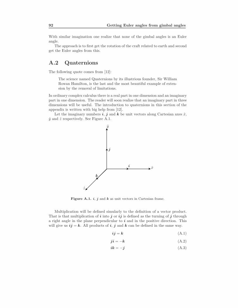
92 Getting Euler angles from gimbal angles
With similar imagination one realize that none of the gimbal angles is an Eulerangle.
The approach is to first get the rotation of the craft related to earth and secondget the Euler angles from this.
A.2 QuaternionsThe following quote comes from [12]:
The science named Quaternions by its illustrious founder, Sir WilliamRowan Hamilton, is the last and the most beautiful example of exten-sion by the removal of limitations.
In ordinary complex calculus there is a real part in one dimension and an imaginarypart in one dimension. The reader will soon realize that an imaginary part in threedimensions will be useful. The introduction to quaternions in this section of theappendix is written with big help from [12].
Let the imaginary numbers i, j and k be unit vectors along Cartesian axes x,y and z respectively. See Figure A.1.
x
y
z
i
j
k
Figure A.1. i, j and k as unit vectors in Cartesian frame.
Multiplication will be defined simularly to the definition of a vector product.That is that multiplication of i into j or ij is defined as the turning of j througha right angle in the plane perpendicular to i and in the positive direction. Thiswill give us ij = k. All products of i, j and k can be defined in the same way.
ij = k (A.1)
ji = −k (A.2)
ik = −j (A.3)
A.2 Quaternions 93
ki = j (A.4)
jk = i (A.5)
kj = −i (A.6)
The associative law of multiplication is assumed to be applicable on this aspectof multiplication. This means that it is indifferent in what way operations aregrouped as long as the order is not changed. For example i(jk) = (ij)k = ijk.Since ij = k, we have i(ij) = ik = −j. From this the square of a unit vector canbe defined by
i(ij) = (ii)j = i2j
∴ i2j = −j,
i2 = −1
(A.7)
Similarlyj2 = −1 (A.8)
k2 = −1 (A.9)
Any vector can be separated into the product of a tensor (scalar gain) and a unitvector. Let α be a vector parallel to i containing a units and β a vector parallelto j containing b units. The traditional laws of numerical multiplication will beused whenever numerical quantities are mixed with vectors.
α = ai
β = bj
αβ = abij
α2 = (ai)(ai) = a2i2 = −α2
(A.10)
The equations above show the possibility to introduce tensors whenever wanted.Therefore it is enough to direct the attention to unit vectors.
Now let α, β be unit vectors not perpendicular to each other. Let θ be theangle from α to β. Let γ be the unit vector perpendicular to α and in the planedefined by α and β. Let ε be the unit vector perpendicular to α, β and γ as inFigure A.2. In Figure A.2 let OA and OB be the vectors from origo to A andB respectively. Since α and β both are unit vectors we have OA = α cos θ andOB = γ sin θ. With γ, β and ε corresponding to j, i and −k respectively thefollowing is given:
α = β cos θ + γ sin θ (A.11)
αβ = (β cos θ + γ sin θ)β =
= β2 cos θ + γβ sin θ

94 Getting Euler angles from gimbal angles
α
β
γ
θ
ε
A
B
O
Figure A.2.
But according to (A.2) and (A.7) γβ = ε and β2 = −1 so
αβ = − cos θ + ε sin θ (A.12)
If α and β are not unit vectors, but contain a and b units respectively, the productis according to (A.10)
αβ = ab(− cos θ + ε sin θ) (A.13)
The quotient βα is defined such that when it operates on α it produces β.
β
αα = β (A.14)
The quotient βα is therefore the multiplier which, operating on β cos θ +γ sin θ (α
according to (A.11)), produces β. But with cos θ + ε sin θ operating on α we have
(cos θ+ε sin θ)(β cos θ+γ sin θ) = β cos2 θ+(γ+εβ) sin θ cos θ+εγ sin2 θ (A.15)
According to (A.4) and (A.6) εβ = −γ and εγ = β. This inserted into (A.15)gives
(cos θ + ε sin θ)(β cos θ + γ sin θ) = β cos2 θ + β sin2 θ = β (A.16)
Combining this with (A.14) gives
β
α= cos θ + ε sin θ (A.17)
Since βα operating on α causes it to become β it is clear that it is an operator
of the same character as −k or ε. While −k or ε would turn α through a rightangle, β
α or cos θ + ε sin θ turns it in the same direction, only through the angle θ.The expression cos θ + ε sin θ is defined as the versor through the angle θ.
A.2 Quaternions 95
Looking at (A.10) again gives the quotient of two non unit vectors β and αcontaining b and a units respectively.
β
α=
b
a(cos θ + ε sin θ) (A.18)
Apparently the product or quotient of two vectors may be expressed as theproduct of a tensor and a versor. Sir William Hamilton named this product aQuaternion.[12]
Every quaternion, q, can be written in polar form.
q =√
Nq(cos θ + q sin θ) (A.19)
where q is a unit vector and Nq is the norm of q. The basic algebraic form for aquaternion, q, is though
q = 1q0 + iq1 + jq2 + kq3 (A.20)
The following equations describes the relation between the two forms.
Nq = q20 + q2
1 + q22 + q2
3 , cos θ =q0√Nq
, sin θ =
√q21 + q2
2 + q23√
Nq
If Nq = 1 the quaternion is called a unit quaternion. Hamilton defined S(q) = q0
as the scalar part and V (q) = iq1 + jq2 + kq3 as the vector part of the quaternionq. That is
q = S(q) + V (q) (A.21)
By analogy with complex numbers the conjugate of q is
q = S(q) − V (q) (A.22)
If a quaternion, q has a nonzero norm, Nq its inverse is defined as
q−1 =q
Nq(A.23)
which gives that
qq−1 =(S(q) + V (q))(S(q) − V (q))
Nq
=S(q)2 − V (q)2
Nq
=q20 − (iq1 + jq2 + kq3)2
Nq= ...
=q20 − (−q2
1 − q22 − q2
3)Nq
= 1
(A.24)
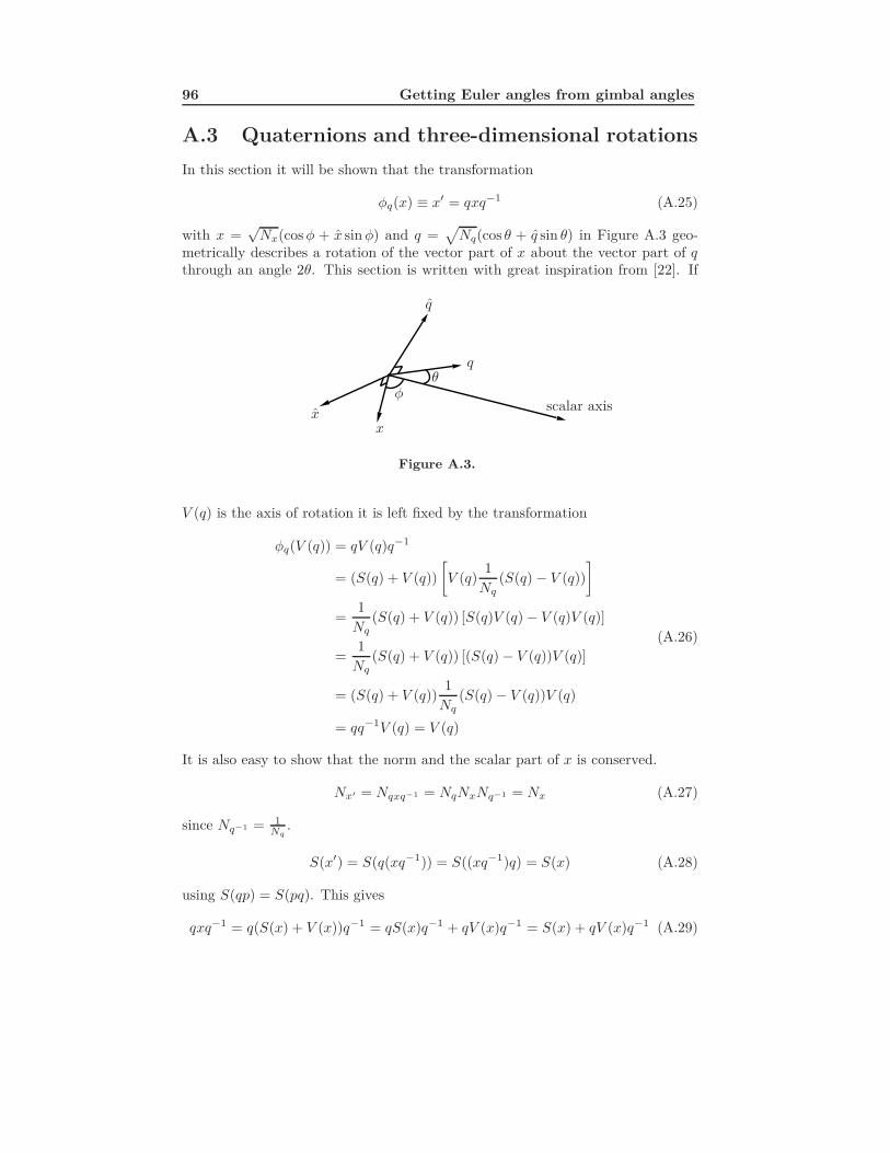
96 Getting Euler angles from gimbal angles
A.3 Quaternions and three-dimensional rotationsIn this section it will be shown that the transformation
φq(x) ≡ x′ = qxq−1 (A.25)
with x =√Nx(cosφ + x sinφ) and q =
√Nq(cos θ + q sin θ) in Figure A.3 geo-
metrically describes a rotation of the vector part of x about the vector part of qthrough an angle 2θ. This section is written with great inspiration from [22]. If
xx
q
qθ
φscalar axis
Figure A.3.
V (q) is the axis of rotation it is left fixed by the transformation
φq(V (q)) = qV (q)q−1
= (S(q) + V (q))[V (q)
1Nq
(S(q) − V (q))]
=1Nq
(S(q) + V (q)) [S(q)V (q) − V (q)V (q)]
=1Nq
(S(q) + V (q)) [(S(q) − V (q))V (q)]
= (S(q) + V (q))1Nq
(S(q) − V (q))V (q)
= qq−1V (q) = V (q)
(A.26)
It is also easy to show that the norm and the scalar part of x is conserved.
Nx′ = Nqxq−1 = NqNxNq−1 = Nx (A.27)
since Nq−1 = 1Nq
.
S(x′) = S(q(xq−1)) = S((xq−1)q) = S(x) (A.28)
using S(qp) = S(pq). This gives
qxq−1 = q(S(x) + V (x))q−1 = qS(x)q−1 + qV (x)q−1 = S(x) + qV (x)q−1 (A.29)
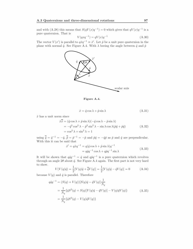
A.3 Quaternions and three-dimensional rotations 97
and with (A.28) this means that S(qV (x)q−1) = 0 which gives that qV (x)q−1 is apure quaternion. That is
V (qxq−1) = qV (x)q−1 (A.30)The vector V (x′) is parallel to qxq−1 ≡ x′. Let p be a unit pure quaternion in theplane with normal q. See Figure A.4. With λ beeing the angle between q and p
x′
x
p
2θq
λ
scalar axis
Figure A.4.
x = q cosλ + p sinλ (A.31)
x has a unit norm sincexx = (q cosλ + p sinλ)(−q cosλ− p sinλ)
= −q2 cos2 λ− p2 sin2 λ− sinλ cosλ(pq + pq)
= cos2 λ + sin2 λ = 1
(A.32)
using q = q−1 = −q, p = p−1 = −p and pq = −qp as p and q are perpendicular.With this it can be said that
x′ = qxq−1 = q(q cosλ + p sinλ)q−1
= qqq−1 cosλ + qpq−1 sinλ(A.33)
It will be shown that qqq−1 = q and qpq−1 is a pure quaternion which revolvesthrough an angle 2θ about q. See Figure A.4 again. The first part is not very hardto show.
V (V (q)q) =12[V (q)q + qV (q)] =
12[V (q)q − qV (q)] = 0 (A.34)
because V (q) and q is parallel. Therefore
qqq−1 = (S(q) + V (q))[S(q)q − qV (q)]1Nq
=1Nq
qS2(q) + S(q)[V (q)q − qV (q)] − V (q)qV (q)
=1Nq
qS2(q) − V (q)qV (q)
(A.35)
98 Getting Euler angles from gimbal angles
But V −1(q) = −V (q)NV (q)
which gives
V (q)qV (q) = −NV (q)V (q)qV −1(q) = −NV (q)q (A.36)
This with (A.35) gives the wanted relation
qqq−1 =1Nq
[S2(q) + NV (q)]q = q (A.37)
The second part will be shown by using a similar approach.
qpq−1 = (S(q) + V (q))[p(S(q) − V (q))]1Nq
=1Nq
pS2(q) + S(q)[V (q)p− pV (q)] − V (q)pV (q)(A.38)
But V (q) and p are perpendicular and V (q)p = −pV (q).
V (q)pV (q) = NV (q)p (A.39)
∴ qpq−1 =1Nq
[(S2(q) −NV (q))p + S(q)[V (q)p− pV (q)]] (A.40)
Showing that p′ = qpq−1 is perpendicular to q is the same as showing that p hasbeen rotated about q. To achieve this S[q(pq−1)q] = 0 has to be shown. Our ownassumption of p gives that S(pq) = −S(pq) = 0. So all we need to show is that
S[(V (q)p− pV (q))q] = 0 (A.41)
equivalentlyS[(qp− pq)q] = 0 or S(qpq) = 0 (A.42)
But S(qpq) = S(q2p) = 0 which means that p′ is perpendicular to q. The angle ofrotation can also be determined using
cosφ =S(p′p)√Np′
√Np
= S(p′p) = −S(p′p) = −S[qpq−1p]
= − 1Nq
(S2(q) −NV (q))S(p2) − S(q)Nq
S[V (q)p− pV (q)]p
=1Nq
(S2(q) −NV (q)) − S(q)Nq
S(−V (q) − V (q))
=1Nq
(S2(q) −NV (q))
=1Nq
(Nq cos2 θ −Nq sin2 θ)
= cos 2θ
(A.43)
∴ φ = 2θ (A.44)
A.4 Quaternions in Test Rig Beta 99
Finallyx′ = q cosλ + p′ sinλ (A.45)
where x′ = p cos 2θ+ qp sin 2θ. Note that qp is perpendicular to both q and p. Thiscompletes the proof of qxq−1 describing a 3-dimensional rotation of the vector partof x through an angle 2θ about the vector part of q.
A.4 Quaternions in Test Rig BetaLet the craft’s initial attitude be described as the vector part of the quaternionx0. If the craft’s angle according to the inner gimbal ring is ξ the quaterniondescribing the craft’s attitude can be expressed qξx0q
−1ξ where
qξ =√
Nqξ
(cos
ξ
2+ qξ sin
ξ
2
)(A.46)
and
qξ =
0
j0
(A.47)
Here qξ represents the axis running through the inner gimbal ring, i.e the craft’srotational axis. This axis rotates with the inner gimbal ring around the perpendic-ular axis running through the outer gimbal ring. If the angle between the gimbalrings is ζ the craft’s attitude can be expressed qζqξx0q
−1ξ q−1
ζ where
qζ =√
Nqζ
(cos
ζ
2+ qζ sin
ζ
2
)(A.48)
and
qζ =
0
0k
(A.49)
The axis running through the outer gimbal ring perpendicular to qξ is qζ . Inanalogy with this using ϑ as the angle of the outer gimbal ring in the inertialframe the craft’s attitude can be expressed qϑqζqξx0q
−1ξ q−1
ζ q−1ϑ where
qϑ =√
Nqϑ
(cos
ϑ
2+ qϑ sin
ϑ
2
)(A.50)
and
qϑ =
i
00
(A.51)
Obviously qϑ represents the inertial x-axis. Using x0 = 1 total rotation of thecraft can be expressed as a rather large quaternion expression.
100 Getting Euler angles from gimbal angles
With the quaternion Q = q0 + iq1 + jq2 +kq3 defining the rotation of the craft[13] gives the rather simple transformation to roll, pitch and yaw.
tan(roll) =2(q0q1 + q2q3)
q20 − q2
1 − q22 + q2
3
(A.52)
sin(pitch) = −2(q1q3 − q0q2) (A.53)
tan(yaw) =2(q1q2 + q0q3)
q20 + q2
1 − q22 − q2
3
(A.54)

UpphovsrättDetta dokument hålls tillgängligt på Internet — eller dess framtida ersättare —under 25 år från publiceringsdatum under förutsättning att inga extraordinäraomständigheter uppstår.
Tillgång till dokumentet innebär tillstånd för var och en att läsa, ladda ner,skriva ut enstaka kopior för enskilt bruk och att använda det oförändrat för icke-kommersiell forskning och för undervisning. Överföring av upphovsrätten vid ensenare tidpunkt kan inte upphäva detta tillstånd. All annan användning av doku-mentet kräver upphovsmannens medgivande. För att garantera äktheten, säker-heten och tillgängligheten finns det lösningar av teknisk och administrativ art.
Upphovsmannens ideella rätt innefattar rätt att bli nämnd som upphovsmani den omfattning som god sed kräver vid användning av dokumentet på ovan be-skrivna sätt samt skydd mot att dokumentet ändras eller presenteras i sådan formeller i sådant sammanhang som är kränkande för upphovsmannens litterära ellerkonstnärliga anseende eller egenart.
För ytterligare information om Linköping University Electronic Press se för-lagets hemsida http://www.ep.liu.se/
CopyrightThe publishers will keep this document online on the Internet — or its possi-ble replacement — for a period of 25 years from the date of publication barringexceptional circumstances.
The online availability of the document implies a permanent permission foranyone to read, to download, to print out single copies for your own use andto use it unchanged for any non-commercial research and educational purpose.Subsequent transfers of copyright cannot revoke this permission. All other uses ofthe document are conditional on the consent of the copyright owner. The publisherhas taken technical and administrative measures to assure authenticity, securityand accessibility.
According to intellectual property law the author has the right to be men-tioned when his/her work is accessed as described above and to be protectedagainst infringement.
For additional information about the Linköping University Electronic Pressand its procedures for publication and for assurance of document integrity, pleaserefer to its www home page: http://www.ep.liu.se/
c© Mattias ErikssonBjörn Wedell