Performance comparison between Shack-Hartmann and astigmatic hybrid wavefront sensors

Performance comparison between Shack–Hartmannand astigmatic hybrid wavefront sensors

Shane BarwickRocky Mound Engineering, 116 White Pine Court, Macon, Georgia 31216, USA

([email protected])

Received 13 October 2009; accepted 10 November 2009;posted 16 November 2009 (Doc. ID 118365); published 11 December 2009

Simulations on Kolmogorov phase screens are employed to compare the relative performance of an astig-matic hybrid wavefront sensor (AHS) to that of a Shack–Hartmann sensor (SHS). The AHS is shown toimprove phase reconstruction accuracy when the subaperture phase contains significant energy in cur-vature modes and a moderate to high number of photons are collected. Dual use of the AHS and SHSmay extend enhanced reconstruction to low signal levels. The AHS is also shown to have a small benefitfor tilt-only reconstruction when the beam has sufficient power. © 2009 Optical Society of America

OCIS codes: 010.7350, 110.1080, 350.1260.

1. Introduction

A great deal of research is currently being devoted tomeasuring higher-order spatial frequencies of phasedue to the ever expanding utility of wavefront sen-sing in diverse areas like ground-based astronomy,ophthalmology, optical testing, communication sys-tems, and military applications. The most popularwavefront sensor is the Shack–Hartmann sensor(SHS). The SHS samples the tilts (first-order deriva-tives) of the wavefront by imaging subapertures ofthe pupil with a traditional lenslet array and thenmeasuring the spatial shifts of the focal images(FIs) relative to those of an unaberrated wavefront.It effectively finds the best piecewise linear approx-imation of the phase. These measurements can beextended to higher spatial frequencies only by sam-pling the pupil with more subapertures with lensletsof smaller pitch. However, higher sampling densityincurs diminishing returns due to fewer photonsper subaperture, lower signal-to-noise ratio (SNR)at the sensor, and noisier tilt measurements.A solution to this trade-off is to measure the first

and second derivatives of the local phase in the sub-aperture to relax the sampling constraint on the pu-pil by making higher-order estimates of the phase

within the subaperture. Thus, the hybrid SHS wasborn [1–4]. Most hybrid sensors acquire curvaturedata by processing two images. In [1] Paterson andDainty introduced a competing concept, theastigmatic hybrid wavefront sensor (AHS), thatrequires only one image. The AHS differs from theSHS by including an astigmatic element at eachlenslet of the array that adds a phase of

ϕðr; θÞ ¼ qr2 cosð2θ − θ0Þ; ð1Þ

where q and θ0 are adjustable parameters and r and θare polar coordinates of the lenslet pupil. As with theSHS the shift in the FI is still proportional to theaverage local wavefront tilt. However, it was shownin [1] that a simple signal could be calculated from aquad cell at the focal plane that is linear with defocusover a range large enough to be valuable in closed-loop wavefront sensing. This measurement is madepossible because the distribution of the energy inthe FI is sensitive to curvature for an astigmaticlenslet. Thus, defocus and tilt are sampled. The extrainformation creates the possibility of better estima-tion of the local wavefront with a higher-ordersurface.

This concept was generalized in [4]. Let the phaseof the wavefront impinging on the pupil of a lenslethave the following form:

0003-6935/09/366967-06$15.00/0© 2009 Optical Society of America

20 December 2009 / Vol. 48, No. 36 / APPLIED OPTICS 6967

Wðx; yÞ ≈ τp þ τxxþ τyyþ τxxx2 þ τyyy2 þ τxyxy; ð2Þ

where τp is the piston coefficient, τx and τy are the tiltcoefficients, and τc ¼ ðτxy; τyy; τxyÞ are the curvaturecoefficients. Pure defocus is equivalent to a τc ofthe form ðα; α; 0Þ, where α is the defocus coefficient.The distribution of the FI of an astigmatic lensletis actually capable of measuring the general τc viaa complex nonlinear mapping if the FI is sampled fi-nely enough by the sensor. In fact, proof of conceptwas demonstrated in [4] that artificial neural net-work (ANN) processing could resolve τc with a mod-erate sampling of the FI. A sufficient number ofpixels to accomplish this task are already in commonuse in order to increase the accuracy of centroid cal-culations in traditional SHSs. The results in [4] werebased on simple simulations of an individual suba-perture in which the pupil of a lenslet was aberratedwith a wavefront in the form of Eq. (2).In this paper, full simulations of wavefront sensors

in open-loop configurations are used to explore underwhat conditions (sampling density of the pupil aper-ture, number of photons collected per subaperture,and pixel pitch of the sensor at the focal plane) theperformance of the AHS exceeds that of the SHS.In Section 2 the methodology of the simulations isdescribed. In Section 3 an efficient method is dis-cussed to estimate the optimum form of Eq. (1) forthe astigmatic phase at the lenslet and the corre-sponding optimum pixel pitch at the sensor. Finally,Section 4 presents results of the simulations anddiscusses the implications.

2. Methodology for the Simulations

The first step in the simulation is to form the imagesfrom which the measurements of the tilts and curva-ture coefficients are drawn. The input wavefront tothe simulations were synthetic Kolmogorov phasescreens of size 1024 × 1024 that were generated bystandard methods of filtering white noise [5]. For asingle simulation run the phase screen was dividedinto an N ×N grid of subapertures of size 1024=N ×1024=N that were individually imaged by an array oflenslets that were assumed to have square pupils. AFI was obtained for each lenslet using standardFourier optics calculations [6]. The lenslets were as-sumed diffraction limited for the SHS, whereas theastigmatic phase of Eq. (1) was taken into accountfor the AHS. Overlap between the FIs of adjacentlenslets on the sensor was assumed negligible.Summation over square regions was performed onthe resulting FIs to mimic individual pixels of thesensor. These pixel values were then rounded to in-tegers and normalized so that Psub photons were col-lected per subaperture. Poisson noise realizationswere next added to the normalized FIs. It was as-sumed that Poisson noise would be the dominantnoise source at relevant signal levels. The requiredpixels per subimage for the AHS and recent advancesin CCD and CMOS technology should make this as-sumption reasonable. The resulting pixel values

served as the inputs for postprocessing to samplethe tilt and curvature components of the phase.

The initial step in postprocessing for both the AHSand the SHS was to determine the shift of the cen-troid of the FI relative to an unaberrated wavefront.The shifts along each Cartesian axis within the im-age plane are proportional to the wavefront tilt withrespect to that axis. The simple method for comput-ing the tilt from the shift is described below. This stepprovided all the data that can be obtained by the SHSfor subsequent reconstruction since the SHS mea-sures only tilts. In the case of the AHS the FI for eachsubaperture was then numerically shifted in thepostprocessing so that the calculated centroid ofthe FI was coincident with the origin of that subaper-ture in the image plane (or equivalently the originwas shifted to the centroid), and a T × T frame of pix-els that contained most of the energy in the FI wasextracted. The pixel values were calculated with lin-ear interpolation for subpixel accuracy to account forthe fractional portion of the shift in the centroid.These pixel values were normalized to sum to 1 bydividing by their total sum.

The shifts of the FI centroid and the normalizedpixel values of the centered FI served as raw datafor estimating the samples of the first and second de-rivatives of the phase across the pupil. The centeredFI served as inputs to the ANNs, whose outputs werehopefully the curvature coefficients. One ANN wastrained for each of the three curvature coefficients.These ANNs required training on representativedata with known outputs. In general, the trainingsets should contain example data that cover the ex-pected range in separate parameters like noise andturbulence statistics that affect the input. The train-ing-set inputs for the simulation were obtained byprocessing enough phase screens in the previouslydescribed manner so that the centered FIs, as wellas centroid shifts, were collected for over 15,000subaperture images. The desired curvature outputcorresponding to each centered FI was found by com-puting the least-squares second-order polynomialsurface in the form of Eq. (2) that best fit the actualphase in each subaperture of the pupil. This surfacealso provided the least-squares tilts for the subaper-ture. The resulting training sets were put to use initerative backpropagation conjugate-gradient algo-rithms to train the ANNs.

The calculation of the tilts from the centroid shiftswas much simpler. The tilts of the wavefront alongeach axis are approximately linearly related to theshifts of the FI along that axis. The linear depen-dence was estimated empirically by finding thebest-fit lines when the least-squares tilts wereplotted versus the shifts. As expected, the interceptsof the linear fits were generally close to zero, whichsupported the accuracy of this approach for deter-mining the “known” values for the tilts and curvaturecoefficients from the best-fit second-order surfaces.Tilts in the simulations were calculated by multiply-ing the noisy centroid shifts by the best-fit slopes.

6968 APPLIED OPTICS / Vol. 48, No. 36 / 20 December 2009

Once estimates for the tilts and curvature coeffi-cients were in hand for a phase screen, the problemstill remained to reconstruct the phase. The tiltsand curvature coefficients are simply related to thederivatives ð∂W=∂x; ∂W=∂y; ∂2W=∂x2; ∂2W=∂y2; ∂2W=∂x∂yÞ of the local phase Wðx; yÞ through the second-order Taylor series approximation of the subaperturephase. The derivatives in turn can be approximatedby finite differences of a discretized W so that thesampled derivatives and phase estimate points canbe related through a linear matrix equation. Thephase was sampled at the same locations as the mea-surements were taken, namely, the center of eachsubaperture. The least-squares solution to this ma-trix equation provides an estimate of the sampledphase. The form of this equation and efficient algo-rithms for its solution are thoroughly explained in[7] and are not repeated here. In all simulationsthe algorithm that was employed to reconstructthe phase corresponds to finite-difference weightedleast-squares reconstruction with Cholesky decom-position for square apertures in [7]. In the least-squares solution the different tilt and curvature datawere weighted differently to optimize the reconstruc-tion. Empirically finding the optimum weights wasimportant to the AHS results, although the optimumweights varied little with the noise level.

3. Design of the Astigmatic Phase

Obviously the accuracy of reconstruction for AHSwill critically depend on the magnitude of the astig-matism phase q introduced to the lenslet in Eq. (1)and the sampling of the FI, which is determinedby pixel pitch p and the number of pixels Q ¼ T2

dedicated to each centered FI. Running full simula-tions for many different combinations of q and p for agiven Q would require impractical amounts of com-putation time. Thus, iterative optimization algo-rithms are impractical also if they require a fullsimulation to calculate a cost function.Information theory, however, provides an efficient

metric to estimate potential performance for designpurposes. The Fisher information matrix (FIM) is ameasure of the information content of a data set withregards to parameters to be estimated from that dataset [8]. In fact, the minimum possible variances, orCramer–Rao bound (CRB), of unbiased estimatesof the parameters from the data set is given by thediagonal elements of the inverse of the FIM. Inthe present case the data set is the centered FI pixelvalues, and the parameters to be estimated are thecurvature coefficients. Let gm be the mth pixel valueof the centered FI at a noiseless sensor (i.e., the meanvalues of gm) when the wavefront impinging on thelenslet has the form of Wðx; yÞ ¼ τ1x2 þ τ2y2 þ τ3xy.Also, let the actual sensor be dominated by Poissonnoise. Then the element at the jth row and kth col-umn of the FIM F for parameters τc ¼ ðτ1; τ2; τ3Þare given by [8]

Fjk ¼Xm

1gmðτc; q;pÞ

∂gmðτc; q; pÞ∂τj

∂gmðτc; q;pÞ∂τk

ð3Þ

for j, k ¼ 1; 2; 3. The CRB of the estimate of τj satisfies

Varfτjg ≥ ½F−1�jj; ð4Þ

where F−1 is the inverse of F, jj refers to the matrixelement position on the diagonal, and τ denotes esti-mate of τ. The CRB can be computed efficiently. Forthe parameters used in the simulations a brute forcegrid search was undertaken to find the value of q andthe pixel size p that minimized the root mean square(RMS) of the CRBs of the three curvature parametersfor a given Q at the sensor. The CRB was typicallycomputed at τc ¼ ð0; 0; 0Þ for this paper, althoughthe minimization could be taken over a weightedrange of τc that was appropriate for the application.

4. Simulation Results

The AHS is expected to have its maximum advantageover the SHS at a coarse sampling of the pupil aper-ture when the phase in the subaperture can no longerbe well approximated by piecewise two-dimensionallinear polynomials. The SHS is blind to energy that ishigher order than the tilts. The energy in the curva-ture components, nuisance parameters for the SHS,becomes useful information for the AHS. Of course,as the density of this subaperture sampling in-creases, less energy in the phase lies outside the tilts,and the advantage should decrease. The relative per-formance is also noise dependent. If the noise is sosevere that the accuracy in the sampled curvaturecoefficients becomes poor, bad data in leads to baddata out, even at coarse sampling. Another issue isthat the inputs to the ANN depend on accurately cal-culating the centroid of the FI through the centeringprocess. Noise in the tilt measurement is, thus, pro-pagated to the curvature measurements. Since astig-matism tends to spread out the point spread functionof the lenslet, it was found in [1] that increasing themagnitude of the astigmatism created a trade-off intilt sensitivity and defocus sensitivity for a simplequad cell signal and pure defocus and tilt aberra-tions. As is demonstrated, this result does not neces-sarily hold for wavefronts of more complex structureand finer sampling of the FI, which has positive ra-mifications for the use of the AHS.

These issues are well demonstrated by examiningthe results of the simulations with phase screensthat were sampled by a grid of 16 × 16 subapertures.The relevant parameters for the simulation are asfollows. These phase screens were generated to be re-presentative of the Kolmogorov spectrum of turbu-lence with D=r0 ¼ 16, where D is the total width ofthe pupil aperture and r0 is the Fried parameter.Therefore, each subaperture had a width of r0. TheANNs were constructed from 5 hiddens layers withthe total number of neurons being 220. The numberof inputs to the ANNs was 64, which corresponded toa sampling of 8 × 8 pixels on the centered FI at the


sensor. The FIs had little energy outside this area.Since the maximum shift in any subaperture in over600 phase screens and 153,000 subapertures was1.67 pixels (mean shift ≈ 0:23 pixels) in any direction,the maximum number of pixels at the sensor thatwould need to be dedicated to a single subapertureis 144 (12 × 12) for the nonoverlap assumption onthe FI to be well met. For this setup the RMS ofthe CRBs for the curvature coefficients was mini-mized when q ¼ 1:25 and p ¼ 10, where p is givenin normalized terms of matrix elements when theFI was calculated with a zero-padded 1024 × 1024fast Fourier transform from the 64 × 64 subaperturephase. The metric used to measure the quality of thephase reconstruction was the residual RMS errorin the sampled phase estimate relative to theactual phase when sampled at the center of eachsubaperture, or

RRMSE ¼

ffiffiffiffiffiffiffiffiffiffiffiffiffiffiffiffiffiffiffiffiffiffiffiffiffiffiffiffiffiffiffiffiffiffiffiffiffiffiffiffiffiffiPm

PnðWmn − WmnÞ2

rffiffiffiffiffiffiffiffiffiffiffiffiffiffiffiffiffiffiffiffiffiffiPm

PnW2

mn

r : ð5Þ

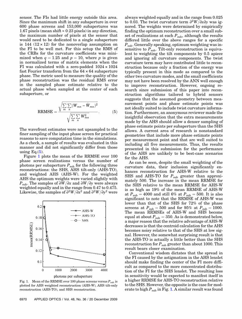
The wavefront estimates were not upsampled to thefiner sampling of the input phase screen for practicalreasons to save computation time in the simulations.As a check, a sample of results was evaluated in thismanner and did not significantly differ from thoseusing Eq.(5).Figure 1 plots the mean of the RRMSE over 100

phase screen realizations versus the number ofphotons per subaperture Psub for the following threereconstructions: the SHS, AHS tilt-only (AHS-TO),and weighted AHS (AHS-W). For the weightedAHS the optimum weights were varied slightly withPsub. The samples of ∂W=∂x and ∂W=∂y were alwaysweighted equally and in the range from 0.47 to 0.475.Likewise, the samples of ∂2W=∂x2 and ∂2W=∂y2 were

always weighted equally and in the range from 0.025to 0.03. The twist curvature term ∂2W=∂x∂y was ig-nored. The weights were determined by empiricallyfinding the optimum reconstruction over a small sub-set of realizations at each Psub, although the resultsdiffered little over the above ranges for a specificPsub. Generally speaking, optimumweighting was in-sensitive to Psub. Tilt-only reconstruction is equiva-lent to weighting the tilt components by 0.5 apieceand ignoring all curvature components. The twistcurvature term may have contributed little to recon-struction because only a fraction of the energy wastypically present in this mode as compared to theother two curvaturemodes, and the small coefficientsmay not have been resolved by the ANN well enoughto improve reconstruction. However, ongoing re-search since submission of this paper into recon-struction algorithms tailored to hybrid sensorssuggests that the assumed geometry between mea-surement points and phase estimate points wasnot ideally suited to include twist curvature informa-tion. Furthermore, an anonymous reviewer made theinsightful observation that the extra measurementsmade by the AHS should allow a denser sampling ofphase estimate points per subaperture than the SHSallows. A current area of research is nonstandardgeometries that include more phase estimate pointsper measurement point and that are well suited toincluding all five measurements. Thus, the resultspresented in this submission for the performanceof the AHS are unlikely to be best-case scenariosfor the AHS.

As can be seen, despite the small weighting of thecurvature data, their inclusion significantly en-hances reconstruction for AHS-W relative to theSHS and AHS-TO for Psub greater than approxi-mately 500. The increase in the mean RRMSE forthe SHS relative to the mean RRMSE for AHS-Wis as high as 19% of the mean RRMSE of AHS-Wat Psub ¼ 4000 and still 6% at Psub ¼ 500. It is alsosignificant to note that the RRMSE of AHS-W waslower than that of the SHS for 72% of the phasescreens at Psub ¼ 500 and for 95% at Psub ¼ 1000.The mean RRMSEs of AHS-W and SHS becomeequal at about Psub ¼ 350. As is demonstrated below,a major reason that the relative advantage of AHS-Wdecreases is that the centroid calculation for the AHSbecomes noisy relative to that of the SHS at low sig-nal. However, the somewhat surprising result is thatthe AHS-TO is actually a little better than the SHSreconstruction for Psub greater than about 1000. Thisresult bears closer examination.

Conventional wisdom dictates that the spread inthe FI caused by the astigmatism in the AHS lensletshould make finding the center of the FI more diffi-cult as compared to the more concentrated distribu-tion of the FI for the SHS lenslet. The resulting lossin sensitivity would be expected to manifest itself ina higher RRMSE for AHS-TO reconstruction relativeto the SHS. However, the opposite is the case for mod-erate to high Psub in Fig. 1. A similar result was found

Fig. 1. Mean of the RRMSE over 100 phase screens versus Psub isplotted for AHS weighted reconstruction (AHS-W), AHS tilt-onlyreconstruction (AHS-TO), and SHS reconstruction.


by van Dam and Lane in [9] when estimating wave-front tilt from the displacement of defocused imagesof Kolmogorov turbulence. A little defocus improvedtilt estimation. They postulated that the defocussmoothed the FI at small scales, which enhancedsubpixel interpolation for maximum-likelihood esti-mates. By the same token, smoothing by the astigma-tism in the present case may reduce filtering effectsdue to spatial integration and sampling by the sensorpixels, which may stabilize the subpixel accuracy ofthe discrete centroid calculation.Another possible advantage of smoothing by the as-

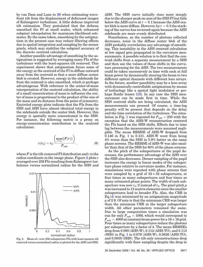
tigmatism is suggested by averaging many FIs of theturbulence with the least-squares tilt removed. Thisexperiment shows that astigmatism forces some ofthe energy at the centroid of the FI to diffuse outwardaway from the centroid so that a more diffuse centerblob is created. However, energy in the sidebands farfrom the centroid is also smoothed, which is perhapsadvantageous. With reference to the center-of-massinterpretation of the centroid calculation, the abilityof a small concentration of mass to influence the cen-ter of mass is proportional to the product of the size ofthemass and its distance from the point of symmetry.Encircled energy plots indicate that the FIs from theSHS and AHS have almost identical total energy inthe sidebands outside the center blob. However, thisenergy is spatially more concentrated in the SHS.For instance, the following metric is a proxy onenergy-concentration contribution to the centroidcalculation:

cðr0Þ ¼ r0

�maxr>r0

fFðrÞg�

Psub; ð6Þ

whereF is the tilt-removedFI distribution and r is theradius coordinate in the image plane. Figure 2 plots caveraged over 256FIs resulting fromKolmogorov tur-bulence versus normalized radius for the SHS and

AHS. The SHS curve initially rises more steeplydue to the sharper peak on-axis of the SHSFI but fallsbelow the AHS curve at r ¼ 0:1 because the AHS cen-ter blob ismore diffuse.However, by r ¼ 0:3 the stack-ing of the curves has reversed again because the AHSsidebands are more evenly distributed.

Nonetheless, as the number of photons collecteddecreases, noise in the diffuse center blob of theAHS probably overwhelms any advantage of smooth-ing. This instability in the AHS centroid calculationat low signal gets propagated to the curvature mea-surements. A possible solution is to first find the cen-troid shifts from a separate measurement by a SHSand then use the values of these shifts in the curva-ture processing for the AHS. The two measurementscould be taken successively in time with each at fullbeam power by dynamically steering the beam to twodifferent optical channels with different lens arrays.In the future, another possibility may be a lens arraywith dynamically controllable astigmatism by meansof technology like a spatial light modulator or per-haps fluidic lenses [10]. In any case the SHS mea-surement can be made first in time. While theSHS centroid shifts are being calculated, the AHSmeasurements can proceed. Of course, a time-lagpenalty will be present that depends on the delayand the time correlation of the turbulence. The simu-lation in Fig. 1 was repeated for Psub ¼ 250 with theexception that the AHS-W reconstruction centeredthe FIs based on the SHS shifts. Effects due to timelag between the measurements were assumed negli-gible. The mean RRMSE of AHS-W dropped from0.146 in Fig. 1 to 0.131. AHS-W went from being4% worse than the SHS to 5.9% better on the samephase screens. The RRMSE of AHS-Wwas also smal-ler than that of the SHS for 80% of the phase screens.

As the pitch of the subapertures at the pupil de-creases, the performance advantage of the AHS overthe SHS also decreases. Denser sampling of the pupilincreases the energy in linear modes of the subaper-ture phase relative to curvature modes. For instance,simulations were repeated with phase screens thatwere sampled by a grid of 32 × 32 subapertures, orfour times as many subapertures and four times asmany estimated phase points. The width of each sub-aperture was now r0=2 instead of r0. The pixel pitch pwas increased to 12matrix elements since the smallersubapertures lead to broader FIs. Also, the CRB inEq.(4) was minimized by an astigmatism magnitudeq of 2.9. Of note is that the minimum CRB was largerthan the minimum CRB at the larger subaperturewidth. All other parameters remained the same.Due to large computation times a simulation wasrun for only Psub ¼ 1000, which would correspond toPsub ¼ 4000at constant beampower for a16 × 16 grid.Four times as many subapertures reduce the photonsper subaperture by a factor of 4. The mean RRMSEsdrop from 0.095 (AHS-W), 0.112 (AHS-TO), and 0.113(SHS) in Fig. 1 to 0.079 (AHS-W), 0.0826 (AHS-TO),and 0.0838 (SHS). The tilt-only reconstructions dropsignificantly with finer sampling despite the drop in

Fig. 2. Mean of c over 256 subaperture FIs with least-squares tiltremoved versus normalized radius is plotted for the AHS and SHS.


SNR at the sensor. ThemeanRRMSE of AHS-TO stillremains slightly lower than that of the SHS, whichindicates good stability in the AHS-W centroid calcu-lation. ThemeanRRMSE of AHS-Walso still remainsthe best of the three at the denser sampling, but theperformance of AHS-W relative to the SHS is betterby only 6%, as opposed to 19% for a 16 × 16 grid. Also,the RRMSEwas lower for AHS-Was compared to theSHS for only 59% of the phase screens, downfrom 99%.

5. Conclusions

Simulations on Kolmogorov phase screens indicatethat AHS can more accurately reconstruct the phaseunder certain conditions relative to a SHS. Specifi-cally, AHS has an advantage in performance whenthe phase local to each subaperture has significantenergy outside of least-squares linear approxima-tions. Also, a moderate to high number of photonsneed to be collected per subaperture to measure cur-vature data with sufficient accuracy to aid in recon-struction. Degradation in AHS performance as thenumber of photons decreases is initially dominatedby noise in the centroid calculation of the FI. Takingtwo successive measurements in time, one with aSHS and one with an AHS, and using the centroidcalculations from the SHS in the AHS-W processing,may make it possible to improve on the performanceof the SHS at low signal levels. Future advances inreconstruction algorithms for hybrid sensors, a rela-tively neglected area of research, should also en-hance the performance of the AHS. Furthermore,results indicate that for sufficient signal the AHSmay have a slight benefit in tilt-only reconstruction

relative to the SHS. Of note is that these tilt-onlyresults were achieved without optimizing the astig-matic phase for that purpose.

I would like to thank the anonymous reviewers forhelpful suggestions and insightful comments thathelped to strengthen this submission.

References1. C. Paterson and J. Dainty, “Hybrid curvature and gradient

wave-front sensor,” Opt. Lett. 25, 1687–1689 (2000).2. S. Barbero, J. Rubinstein, and L. Thibos, “Wavefront sensing

and reconstruction from gradient and Laplacian datameasured with a Hartmann-Shack sensor,” Opt. Lett. 31,1845–1847 (2006).

3. W. Zou, K. Thompson, and J. Rolland, “Differential Shack-Hartmann curvature sensor: local principal curvaturemeasurements,” J. Opt. Soc. Am. A 25, 2331–2337 (2008).

4. S. Barwick, “Detecting higher-order wavefront aberrationswith an astigmatic hybrid wavefront sensor,” Opt. Lett. 34,1690–1692 (2009).

5. E. Johansson and D. Gavel, “Simulation of stellar speckleimaging,” Proc. SPIE 1237, 372–383 (1994).

6. J. W. Goodman, Introduction to Fourier Optics (McGraw-Hill, 1968).

7. S. Barwick, “Least-squares reconstruction for hybrid curva-ture wavefront sensors,” J. Opt. Soc. Am. A (to be published).

8. H. Barrett, C. Dainty, and D. Lara, “Maximum-likelihoodmethods in wavefront sensing: stochastic models and likeli-hood functions,” J. Opt. Soc. Am. A 24, 391–414 (2007).

9. M. A. van Dam and R. G. Lane, “Tip/tilt estimation from de-focused images,” J. Opt. Soc. Am. A 19, 745–752 (2002).

10. R. Marks, D. Mathine, J. Schwiegerling, G. Peyman, andN. Peyghambarian, “Astigmatism and defocus wavefront cor-rection via Zernike modes produced with fluidic lenses,” Appl.Opt. 48, 3580–3587 (2009).


Documents

Performance comparison between Shack-Hartmann and astigmatic hybrid wavefront sensors