Performance analysis based on least squares and extended Kalman filter for localization of static target in wireless sensor networks

1

3

4

5

6

7

8 Q2

9 Q310

11

1 3

1415161718

19202122232425

2 6

4849

50

51

Q1

Q4Q2

Ad Hoc Networks xxx (2014) xxx–xxx

ADHOC 1102 No. of Pages 15, Model 3G

26 September 2014

Q2

Contents lists available at ScienceDirect

Ad Hoc Networks

journal homepage: www.elsevier .com/locate /adhoc

Performance analysis based on least squares and extendedKalman filter for localization of static target in wireless sensornetworks q

http://dx.doi.org/10.1016/j.adhoc.2014.08.0111570-8705/� 2014 Elsevier B.V. All rights reserved.

q This work is partially supported by National Natural ScienceFoundation in China (NSFC) under Grants 61473038 and 61374099. Thiswork is also supported by Program for New Century Excellent Talents inUniversity (NCET-09-0045 and NCET-13-0652), Beijing OutstandingTalents Programme (2012D009011000003), and Beijing Higher EducationYoung Elite Teacher Project (YETP0505).⇑ Corresponding authors.

E-mail addresses: [email protected] (W. Wang), [email protected],[email protected] (H. Ma), [email protected] (Y. Wang), [email protected] (M. Fu).

Please cite this article in press as: W. Wang et al., Performance analysis based on least squares and extended Kalman filter for locaof static target in wireless sensor networks, Ad Hoc Netw. (2014), http://dx.doi.org/10.1016/j.adhoc.2014.08.011

Weidong Wang a, Hongbin Ma b,⇑, Youqing Wang a,⇑, Mengyin Fu b

a College of Information Science and Technology, Beijing University of Chemical Technology, Chinab State Key Laboratory of Intelligent Control and Decision of Complex Systems, School of Automation, Beijing Institute of Technology, China

a r t i c l e i n f o

272829303132333435363738

Article history:Received 29 November 2013Received in revised form 23 June 2014Accepted 17 August 2014Available online xxxx

Keywords:Wireless sensor networksLocalizationLeast squaresExtended Kalman filterPerformance analysis

3940414243444546

a b s t r a c t

Wireless sensor network localization is an essential problem that has attracted increasingattention due to wide demands such as in-door navigation, autonomous vehicle, intrusiondetection, and so on. With the a priori knowledge of the positions of sensor nodes and theirmeasurements to targets in the wireless sensor networks (WSNs), i.e. posterior knowledge,such as distance and angle measurements, it is possible to estimate the position of targetsthrough different algorithms. In this contribution, two commonly-used approaches basedon least-squares and Kalman filter are described and analyzed for localization of one statictarget in the WSNs with distance, angle, or both distance and angle measurements, respec-tively. Noting that the measurements of these sensors are generally noisy of certain degree,it is crucial and interesting to analyze how the accuracy of localization is affected by thesensor errors and the sensor network, which may help to provide guideline on choosingthe specification of sensors and designing the sensor network. In addition, the problemof optimal sensor placement is also addressed to minimize the localization error. To thisend, theoretical analysis have been made for the different methods based on three typicaltypes of measurement noise: bounded noise, uniformly distributed noise, and Gaussianwhite noise. Simulation results illustrate the performance comparison of these differentmethods, the theoretical analysis and simulations and the optimal sensor geometry whichmay be meaningful and guideful in practice.

� 2014 Elsevier B.V. All rights reserved.

47

52
1. Introduction micro-electro-mechanical systems (MEMS) technology, 53
54

55

Wireless sensor networks (WSNs) have attractedworldwide attention with the recent advances in

56

57

58

59

60

61

62

63

64

wireless communications, and digital electronics. A wire-less sensor network consists of lots of low-cost, low-power,multi-functional sensors nodes with sensing, data process-ing, and communicating components, which are denselydeployed to monitor the physical environment coopera-tively [1,2]. WSNs have great potentials for many applica-tions in scenarios such as autonomous vehicles [3],battlefield monitoring [4], target tracking and surveillance[5], intrusion detection [6], natural disaster relief [7], bio-medical health monitoring [8], volcano monitoring [9],and seismic sensing [10]. Target localization is one of themost fundamental tasks for WSNs [11]. As facing cost,

lization

http://dx.doi.org/10.1016/j.adhoc.2014.08.011

mailto:[email protected]




mailto:fumy@ bit.edu.cn

mailto:fumy@ bit.edu.cn


http://www.sciencedirect.com/science/journal/15708705

http://www.elsevier.com/locate/adhoc


65

66

67

68

69

70

71

72

73

74

75

76

77

78

79

80

81

82

83

84

85

86

87

88

89

90

91

92

93

94

95

96

97

98

99

100

101

102

103

104

105

106

107

108

109

110

111

112

113

114

115

116

117

118

119

120

121

122

123

124

125

126

127

128

129

130

131

132

133

134

135

136

137

138

139

140

141

142

143

144

145

146

147

148

149

150

151

152

153

154

155

156

157

158

159

160

161

162

163

164

165

166

167

168

169

170

171

172

173

174

175

176

177

178

179

180

181

182

183

184

185

186

2 W. WangQ2 et al. / Ad Hoc Networks xxx (2014) xxx–xxx


26 September 2014

Q2

power, and other constraints, precise and low-cost localiza-tion is a critical requirement in WSNs.

Many researchers have focused on the problem of local-ization [12–15]. According to [16], localization techniquescan be divided into two categories based on the communi-cation among the sensor nodes: centralized localizationand decentralized localization techniques [17]. For differ-ent mechanisms, we can also divide these methods intorange-based and range-free schemes. The former needsto measure the distance or angle for position estimatingbased on time-of-arrival (TOA) [18], time-difference-of-arrival (TDOA) [19], received signal strength (RSS) [20],or angle-of-arrival (AOA) [21]. For range-free approaches,it is unavailable to get these measurements and they relymostly on such information as proximity, i.e. neighbor con-nectivity, or hop-count in multi-hop WSNs [22,23]. In thispaper, we merely discuss the situation of range-basedschemes.

For localization problem in WSNs, algorithm design anderror analysis are of great importance in wireless sensornetworks. Since we aim at precise localization, what weconcentrate on is not only how to locate the target, but alsothe accuracy degree or the error bound of the localizationresult. With these considerations, one interesting and cru-cial problem is—Can we obtain better localization perfor-mance according to different kinds of measurements orother realistic cases through algorithm selection and sensornetwork design? Obviously the answer to this problem isnot trivial and detailed investigations to this problemmay bring through direct benefits to applications of WSNs.Note that in practice, considering the demands of lowercomplexity and real-time computing, it may not be neces-sary to take all possible algorithms and situations in con-sideration, which may result in unnecessary complexityin computation or implementation.

Several methods were described in [24] through differ-ent measurements such as a distance and a direction, twodirections, or three distances. Least-squares (LS) waswidely used for position estimation [25–30]. A newmethod was presented by splitting the complex least-squares algorithm into a less central precalculation and asimple, distributed subcalculation in [31]. For underwaterwireless sensor networks (UWSN), a novel least-squaresmethod based on energy measurements was proposed in[32]. In [33], Born and Reichenbach presented a techniqueto convert the complex nonlinear Least Squares calculationand distribute the tasks over the network effectively. Kal-man filter can be also used for localization in WSNs[17,34]. Rao and Durrant-Whyte [17] presented a fullydecentralized Kalman filter algorithm which ensured theideal implementation on a parallel processing array. In[34], RF mapping and Kalman filter were used to initializethe position and update the estimation using the distancemeasurements respectively.

For error analysis, Zhang et al. [35] analyzed some pos-sible conditions for unique localization based on distanceor bearing constraints and their combination respectively.Crámer–Rao lower bound (CRLB) is also widely used whichis an algorithm-independent method [36–40]. In [36], theCRLB was given under anchored localization and anchor-free localization. Literature [38] dealt with the localization

Please cite this article in press as: W. Wang et al., Performance analysisof static target in wireless sensor networks, Ad Hoc Netw. (2014), http

errors in distance-based on-dimensional sensor networks.The fundamental behaviors of localization errors were ana-lyzed when new measurement, new sensor, or new anchoris added to the existing sensor networks. In [39], the opti-mal sensor placement problem was discussed by minimiz-ing the CRLB of the localization error in heterogeneoussensor networks.

However, few of these above-mentioned publicationshave focused on the error analysis and comparison of theaccuracy based on different measurements and algorithms.To address the formerly mentioned crucial problem ofalgorithm selection and network design based on localiza-tion accuracy analysis, in this paper, we contribute togiving the full description of the two typical methods(least-squares and Kalman filter) by using different mea-surements for target localization in WSNs. We also maketheoretical analysis to yield the mean and covariance ofthe estimation for these different cases while facing threetypes of measurement noise, which is not related to thetrue distance between the sensor nodes and the unknowntarget or related to the distance, respectively. With thetheoretical analysis, the optimal sensor placement forthe basic 3-sensor case is discussed. Then we comparethe accuracy of these different situations through furthersimulations and analyze the relationship between theaccuracy and the detection region. We also simulate thecase where the measurement noise is related to the truedistance between the senor nodes and the unknown target.In addition, the errors of 4 typical types of sensor deploy-ment are compared to find out a more reasonable sensorplacement in practice.

The error analysis of these two methods (least-squaresand Kalman filter) has been made in [41], where we onlydiscuss the case where the measurement noise is notrelated to the distance and the proof details are notgiven. This article could be considered an extended ver-sion of our conference paper [41]. Compared with [41],the following additional contributions are made in thispaper: first, the full mathematical proofs and more dis-cussions are made for least-squares method where themeasurement noise is not related to the distance; second,the case where the measurement noise is related to thedistance is discussed, especially for Kalman filter method,the estimation and error analysis are sufficiently madefor the three models (distance, angle, distance and angle)respectively; in addition, the comparison of the simula-tions and the theoretical analysis have been added; atlast, the optimal sensor placement problem is discussedin this paper.

The remainder of this paper is organized as follows:Problem formulation is first discussed in Section 2 withthe description of information of the sensor nodes andtheir available measurements; Section 3 describes theleast-squares and Kalman filter algorithms for localizationwith different measurements, and we present theoreticalanalysis for the methods mentioned above based on threetypes of noise with different characteristics in Section 4;Section 6 gives the optimal sensor placement for basic3-sensor case under LS� l model; Section 7 shows the sim-ulation results for performance comparison; finally, someconcluding remarks are given in Section 8.

based on least squares and extended Kalman filter for localization://dx.doi.org/10.1016/j.adhoc.2014.08.011


187

188

189

190

191

192

193

194

195

196

197

198

199

200

201

202

203

204

205

206

207

208

209

210

211

212

213

214

215

216

217

218

219

220

221

222223

225225

226

227

228

229

230

231

232

233234

236236

237

238

239

240

241

242

243

244

245246

248248

249

250

251

252

253

254

255

256

257

258

259

260

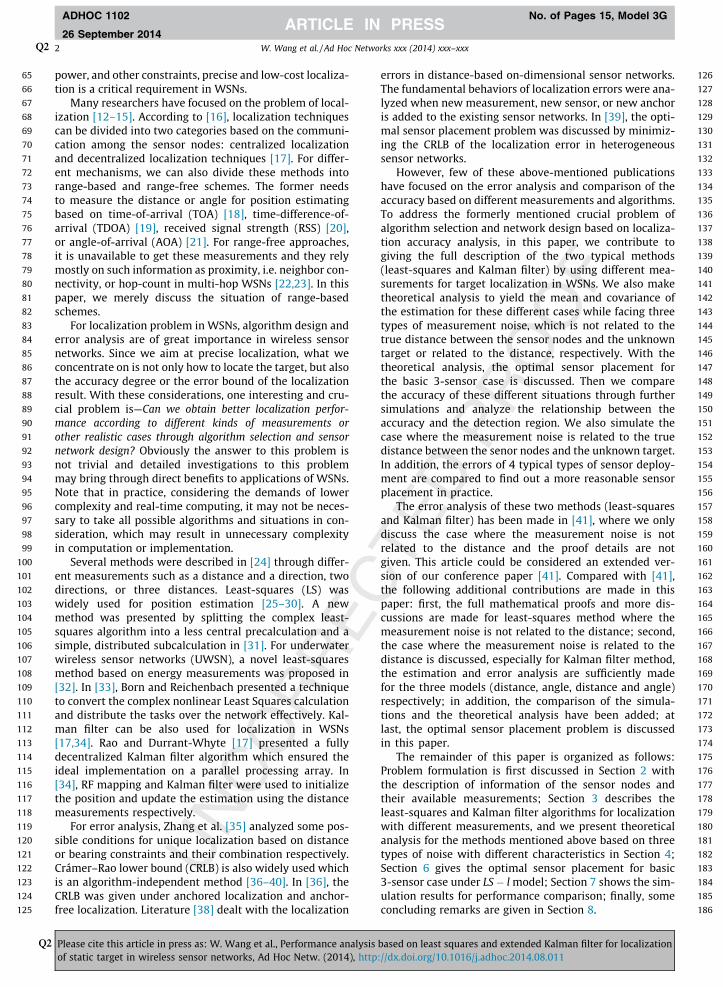
Fig. 1. Case 1: distance measurements only.

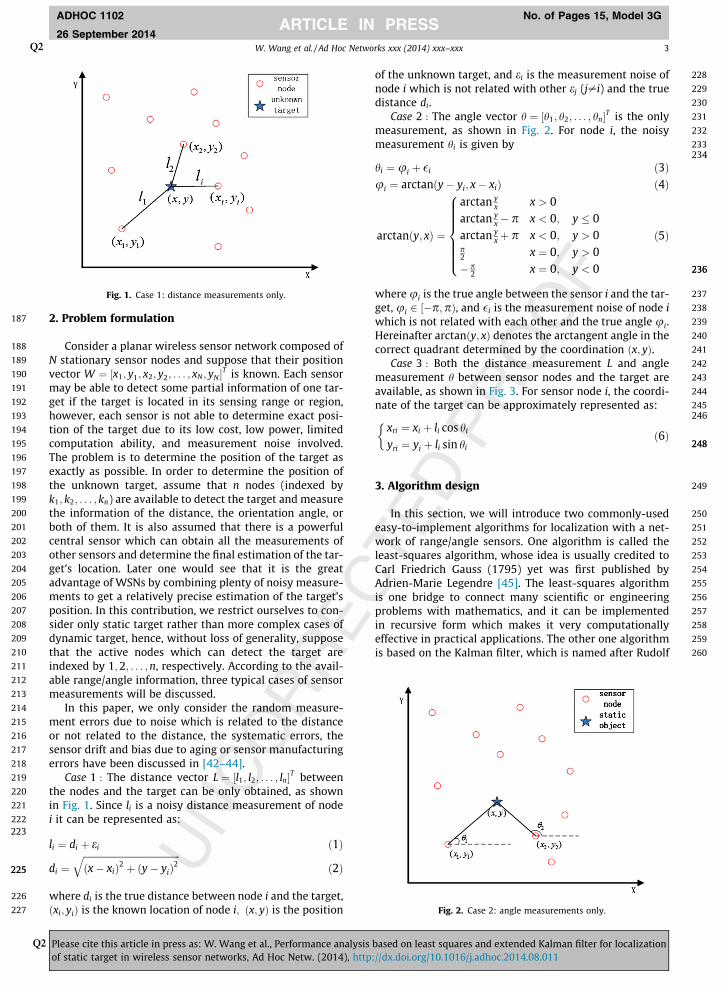
Fig. 2. Case 2: angle measurements only.

W. WangQ2 et al. / Ad Hoc Networks xxx (2014) xxx–xxx 3


26 September 2014

Q2

2. Problem formulation

Consider a planar wireless sensor network composed ofN stationary sensor nodes and suppose that their positionvector W ¼ ½x1; y1; x2; y2; . . . ; xN; yN�

T is known. Each sensormay be able to detect some partial information of one tar-get if the target is located in its sensing range or region,however, each sensor is not able to determine exact posi-tion of the target due to its low cost, low power, limitedcomputation ability, and measurement noise involved.The problem is to determine the position of the target asexactly as possible. In order to determine the position ofthe unknown target, assume that n nodes (indexed byk1; k2; . . . ; kn) are available to detect the target and measurethe information of the distance, the orientation angle, orboth of them. It is also assumed that there is a powerfulcentral sensor which can obtain all the measurements ofother sensors and determine the final estimation of the tar-get’s location. Later one would see that it is the greatadvantage of WSNs by combining plenty of noisy measure-ments to get a relatively precise estimation of the target’sposition. In this contribution, we restrict ourselves to con-sider only static target rather than more complex cases ofdynamic target, hence, without loss of generality, supposethat the active nodes which can detect the target areindexed by 1;2; . . . ;n, respectively. According to the avail-able range/angle information, three typical cases of sensormeasurements will be discussed.

In this paper, we only consider the random measure-ment errors due to noise which is related to the distanceor not related to the distance, the systematic errors, thesensor drift and bias due to aging or sensor manufacturingerrors have been discussed in [42–44].

Case 1 : The distance vector L ¼ ½l1; l2; . . . ; ln�T betweenthe nodes and the target can be only obtained, as shownin Fig. 1. Since li is a noisy distance measurement of nodei it can be represented as:

li ¼ di þ ei ð1Þ

di ¼ffiffiffiffiffiffiffiffiffiffiffiffiffiffiffiffiffiffiffiffiffiffiffiffiffiffiffiffiffiffiffiffiffiffiffiffiffiffiffiffiffiffiðx� xiÞ2 þ ðy� yiÞ

2q

ð2Þ

where di is the true distance between node i and the target,ðxi; yiÞ is the known location of node i; ðx; yÞ is the position


of the unknown target, and ei is the measurement noise ofnode i which is not related with other ej (j–i) and the truedistance di.

Case 2 : The angle vector h ¼ ½h1; h2; . . . ; hn�T is the onlymeasurement, as shown in Fig. 2. For node i, the noisymeasurement hi is given by

hi ¼ ui þ �i ð3Þui ¼ arctanðy� yi; x� xiÞ ð4Þ

arctanðy; xÞ ¼

arctan yx x > 0

arctan yx � p x < 0; y � 0

arctan yx þ p x < 0; y > 0

p2 x ¼ 0; y > 0� p

2 x ¼ 0; y < 0

8>>>>>><>>>>>>:ð5Þ

where ui is the true angle between the sensor i and the tar-get, ui 2 ½�p;pÞ, and �i is the measurement noise of node iwhich is not related with each other and the true angle ui.Hereinafter arctanðy; xÞ denotes the arctangent angle in thecorrect quadrant determined by the coordination ðx; yÞ.

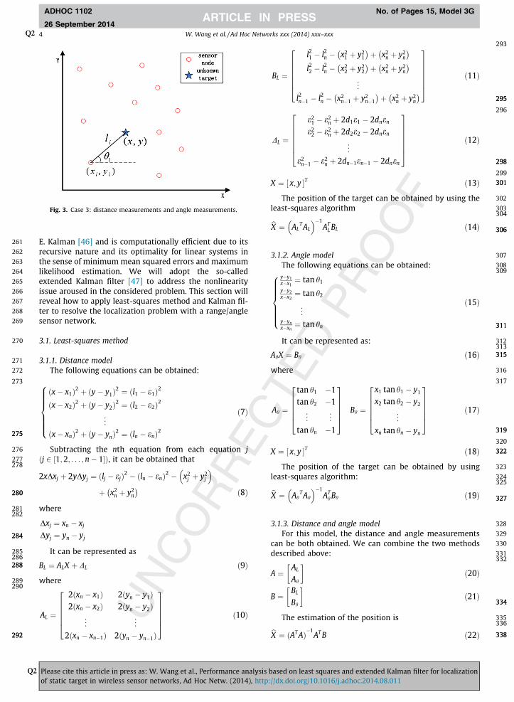
Case 3 : Both the distance measurement L and anglemeasurement h between sensor nodes and the target areavailable, as shown in Fig. 3. For sensor node i, the coordi-nate of the target can be approximately represented as:

xri ¼ xi þ li cos hi

yri ¼ yi þ li sin hi

�ð6Þ

3. Algorithm design

In this section, we will introduce two commonly-usedeasy-to-implement algorithms for localization with a net-work of range/angle sensors. One algorithm is called theleast-squares algorithm, whose idea is usually credited toCarl Friedrich Gauss (1795) yet was first published byAdrien-Marie Legendre [45]. The least-squares algorithmis one bridge to connect many scientific or engineeringproblems with mathematics, and it can be implementedin recursive form which makes it very computationallyeffective in practical applications. The other one algorithmis based on the Kalman filter, which is named after Rudolf



261

262

263

264

265

266

267

268

269

270

271

272

273

275275

276

277278

280280

281282

284284

285286288288

289290

292292

293

295295

296

298298

299301301

302

303304

306306

307

308309

311311

312313315315

316

317

319319

320322322

323

324325

327327

328

329

330

331332

334334

335336

338338

Fig. 3. Case 3: distance measurements and angle measurements.



26 September 2014

Q2

E. Kalman [46] and is computationally efficient due to itsrecursive nature and its optimality for linear systems inthe sense of minimum mean squared errors and maximumlikelihood estimation. We will adopt the so-calledextended Kalman filter [47] to address the nonlinearityissue aroused in the considered problem. This section willreveal how to apply least-squares method and Kalman fil-ter to resolve the localization problem with a range/anglesensor network.

3.1. Least-squares method

3.1.1. Distance modelThe following equations can be obtained:

ðx� x1Þ2 þ ðy� y1Þ2 ¼ ðl1 � e1Þ2

ðx� x2Þ2 þ ðy� y2Þ2 ¼ ðl2 � e2Þ2

..

.

ðx� xnÞ2 þ ðy� ynÞ2 ¼ ðln � enÞ2

8>>>>><>>>>>:ð7Þ

Subtracting the nth equation from each equation jðj 2 ½1;2; . . . ;n� 1�Þ, it can be obtained that

2xDxj þ 2yDyj ¼ ðlj � ejÞ2 � ðln � enÞ2 � x2j þ y2

j

� �þ x2

n þ y2n

� �ð8Þ

where

Dxj ¼ xn � xj

Dyj ¼ yn � yj

It can be represented as

BL ¼ ALX þ DL ð9Þ

where

AL ¼

2ðxn � x1Þ 2ðyn � y1Þ2ðxn � x2Þ 2ðyn � y2Þ

..

. ...

2ðxn � xn�1Þ 2ðyn � yn�1Þ

266664377775 ð10Þ


BL ¼

l21 � l2n � x21 þ y2

1

� �þ x2

n þ y2n

� �l22 � l2n � x2

2 þ y22

� �þ x2

n þ y2n

� �...

l2n�1 � l2n � x2

n�1 þ y2n�1

� �þ x2

n þ y2n

� �

2666664

3777775 ð11Þ

DL ¼

e21 � e2

n þ 2d1e1 � 2dnen

e22 � e2

n þ 2d2e2 � 2dnen

..

.

e2n�1 � e2

n þ 2dn�1en�1 � 2dnen

2666664

3777775 ð12Þ

X ¼ x; y½ �T ð13Þ

The position of the target can be obtained by using theleast-squares algorithm

bX ¼ ALT AL

� ��1AT

L BL ð14Þ

3.1.2. Angle modelThe following equations can be obtained:

y�y1x�x1¼ tan h1

y�y2x�x2¼ tan h2

..

.

y�ynx�xn¼ tan hn

8>>>>><>>>>>:ð15Þ

It can be represented as:

AhX ¼ Bh ð16Þ

where

Ah ¼

tan h1 �1tan h2 �1

..

. ...

tan hn �1

266664377775 Bh ¼

x1 tan h1 � y1

x2 tan h2 � y2

..

.

xn tan hn � yn

266664377775 ð17Þ

X ¼ x; y½ �T ð18Þ

The position of the target can be obtained by usingleast-squares algorithm:

bX ¼ AhT Ah

� ��1AT

hBh ð19Þ

3.1.3. Distance and angle modelFor this model, the distance and angle measurements

can be both obtained. We can combine the two methodsdescribed above:

A ¼AL

Ah

� ð20Þ

B ¼BL

Bh

� ð21Þ

The estimation of the position is

bX ¼ ðAT AÞ�1

AT B ð22Þ



339

340

341

342343345345

346

347

348

349350352352

353

354

355

356357

359359

360

362362

363

364

365

366

367368

370370

371

372

373374

376376

377

378

379

380

381382

384384

385386

388388

389390

392392

393394

396396

397398400400

401

402

403

404

405

406

407

408409

411411

412413

415415

416

417

418

419420

422422

423

424

425

426

427428

430430

431

432

433

434

435436

438438

439

440

441

442443

445445

446

447

448

449

450451



26 September 2014

Q2

3.2. Kalman filter method

3.2.1. Distance modelWe assume that the distance measurement L can be

only obtained. The state model of the system is

Xkþ1 ¼ AXk ð23Þ

where Xk ¼ ½xrk; yrk�T represents the position vector of

the target which is calculated by node k. Here

A ¼ I2 ¼1 00 1

� . And the observation model of the system

can be represented by

Zk ¼ hkðXkÞ þ vk ð24Þ

where Zk ¼ lk, the actual measurement of node k, and vk ismeasurement noise of node k whose covariance is Rk. Theobservation function hkðXkÞ and corresponding JacobianHk derived from Eq. (2) are given as follows

hkðXkÞ ¼ffiffiffiffiffiffiffiffiffiffiffiffiffiffiffiffiffiffiffiffiffiffiffiffiffiffiffiffiffiffiffiffiffiffiffiffiffiffiffiffiffiffiffiffiffiffiffiffiffiðxrk � xkÞ2 þ ðyrk � ykÞ

2q

ð25Þ

Hk ¼xrk � xkffiffiffiffiffiffiffiffiffiffiffiffiffiffiffiffiffiffiffiffiffiffiffiffiffiffiffiffiffiffiffiffiffiffiffiffiffiffiffiffiffiffiffiffiffiffiffiffiffi

ðxrk � xkÞ2 þ ðyrk � ykÞ2

q yrk�ykffiffiffiffiffiffiffiffiffiffiffiffiffiffiffiffiffiffiffiffiffiffiffiffiffiffiffiffiffiffiðxrk�xkÞ2þðyrk�ykÞ2p

" #ð26Þ

For this state-space model, it is ready to apply theextended Kalman filter (EKF) which consists of two conse-quent stages at step k (k ¼ 1;2; . . . ;n).

Time update. Before the new measurement Zk arrives,we can make predictions as follows. Predicted state vector:bXkjk�1 ¼ AbXk�1jk�1 ð27Þ

where bXk�1jk�1 is the state estimation of sensork� 1; bXkjk�1 is the predicted state of sensor k.

Predicted error covariance:

Pkjk�1 ¼ APk�1jk�1AT ð28Þ

where Pk�1jk�1 is the error covariance of bXk�1jk�1 and Pkjk�1

is the error covariance of bXkjk�1.Measurement update. With new measurement Zk, we

can update bXkjk and Pkjk as follows.Measurement residual:

~yk ¼ Zk � hkbXkjk�1

� �ð29Þ

Residual covariance of ~yk:

Sk ¼ HkPkjk�1HTk þ Rk ð30Þ

Kalman gain:

Kk ¼ Pkjk�1HTk S�1

k ð31Þ

Updated state estimate:bXkjk ¼ bXkjk�1 þ Kk~yk ð32Þ

Updated estimate covariance:

Pkjk ¼ ðI � KkHkÞPkjk�1 ð33Þ

453453

3.2.2. Angle modelSuppose that h is the only measurement that can be

obtained. We also need to locate the target through the


observation of the n sensor nodes whose positions are apriori known.

The initial value of the target X2 ¼ ½xr2; yr2�T is deter-

mined by the measurements h1 and h2 from the first twosensors:

tan h1 ¼yr2 � y1

xr2 � x1ð34Þ

tan h2 ¼yr2 � y2

xr2 � x2ð35Þ

then xr2 and yr2 can be given by

xr2 ¼y1 � y2 � ðx1 tan h1 � x2 tan h2Þ

ðtan h2 � tan h1Þð36Þ

yr2 ¼ðx2 � x1Þ tan h1 tan h2 þ y1 tan h2 � y2 tan h1

tan h2 � tan h1ð37Þ

where ðx1; y1Þ and ðx2; y2Þ are the coordinates of the firsttwo sensor nodes.

The state model of the target and the observation modelof sensor k ðk P 3Þ can be described by

Xk ¼ AXk�1 ð38ÞZk ¼ hkðXkÞ þ vk ð39Þ

where Xk ¼ ½xrk; yrk�T is the position of the target that calcu-

lated by node k, Zk ¼ hk denotes the measurement of nodek, vk is the measurement noise of node k with covarianceQk, and A ¼ I2. The observation function hkðXkÞ and corre-sponding Jacobian Hk are:

hkðXkÞ ¼ arctanðyrk � yk; xrk � xkÞ ð40Þ

Hk ¼yk � yrk

ðxrk � xkÞ2 þ ðyrk � ykÞ2

xrk�xk

ðxrk�xkÞ2þðyrk�ykÞ2

� ð41Þ

Then Kalman filter can be used for state estimationthrough Eqs. (27)–(33).

3.2.3. Distance and angle modelWe assume that both of the distance and angle can be

measured. The initial value of the target X1 ¼ ½xr1; yr1�T is

xr1 ¼ x1 þ l1 cos h1

yr1 ¼ y1 þ l1 sin h1

�ð42Þ

where ðx1; y1Þ is the coordinate of the first sensor nodewhose measurements are l1 and h1.

The state model of the target and the observation modelof sensor k ðk P 2Þ:Xk ¼ AXk�1 ð43ÞZk ¼ hkðXkÞ þ vk ð44Þ

where Xk ¼ ½xrk; yrk�T is the position of the target that is cal-

culated by node k, Zk ¼ ½lk; hk�T denotes the measurement ofnode k, vk is the measurement noise of node k with covari-ance Q k, and A ¼ I2. The observation function hkðXkÞ andcorresponding Jacobian Hk are

hkðXkÞ¼ffiffiffiffiffiffiffiffiffiffiffiffiffiffiffiffiffiffiffiffiffiffiffiffiffiffiffiffiffiffiffiffiffiffiffiffiffiffiffiffiffiffiffiffiffiffiffiðxrk�xkÞ2þðyrk�ykÞ

2qarctanðyrk�yk;xrk�xkÞ

" #

Hk¼

xrk�xkffiffiffiffiffiffiffiffiffiffiffiffiffiffiffiffiffiffiffiffiffiffiffiffiffiffiffiffiffiffiffiffiffiffiffiffiffiffiffiffiffiffiffiffiffiffiffiðxrk�xkÞ2þðyrk�ykÞ

2q yrk�ykffiffiffiffiffiffiffiffiffiffiffiffiffiffiffiffiffiffiffiffiffiffiffiffiffiffiffiffiffiffiffiffiffiffiffiffiffiffiffiffiffiffiffiffiffiffiffi


qyk�yrk


xrk�xk


2666437775



454

455

456

457

458

459

460

461

462

463

464465

467467

468

470470

471

472473

475475

476

477

478

479

480

481

482

483

484485

487487

488

489490

492492

493

494

496496

497

498

499500

502502

503

504

505506



26 September 2014

Q2

Then Eqs. (27)–(33) can be used for position estimation.

4. Theoretical analysis

For convenience, we use eX ¼ bX � X to denote the esti-mation error of the position of the unknown target.

4.1. Least squares

4.1.1. Distance model

Proposition 4.1. ATL AL in Eq. (14) is an invertible matrix only

if all the sensors are not deployed in a straight line.

508508

509510

512512

513514

516516

517

518

519

520

521

522

523

524

525

526

527

Proof. As for (10), ATL AL can be written as:

ATL AL ¼ 4

Pn�1i¼1 ðxn � xiÞ2

Pn�1i¼1 ðxn � xiÞðyn � yiÞPn�1

i¼1 ðxn � xiÞðyn � yiÞPn�1

i¼1 ðyn � yiÞ2

" #

116

ATL AL

¼Xn�1

i¼1

ðxn�xiÞ2Xn�1

i¼1

ðyn�yiÞ2�

Xn�1

i¼1

ðxn�xiÞðyn�yiÞ !2

¼X

16i;j6n�1i–j

ðxn�xiÞðyn�yjÞ�ðxn�xjÞðyn�yiÞ� �2 P 0

If ATL AL

¼ 0, then for all i; j 2 ½1;n� 1�; i–j, the follow-ing equation holds

yn � yi

xn � xi¼

yn � yj

xn � xjð45Þ

Thus if all the sensors are not deployed in a straight line,j AT

L AL j> 0; ATL AL is an invertible matrix.

In practical applications, it is meaningless to place therange sensors in a straight line. Therefore, in the followingtheorems, we suppose that matrix AT

L AL is invertible. �

528

529

530

531

532

533

534535

537537

538

539540

Theorem 4.1. Consider the distance model, and suppose thatthe noise ei of sensor node i is Gaussian noise with zero meanand covariance r2

i [48], i.e. ei � Nð0;r2i Þ. Then for the least

squares algorithm presented in Section 3.1.1, we have

EDL ¼ r21 � r2

n;r22 � r2

n; . . . ;r2n�1 � r2

n

� �T ð46Þ

EeX ¼ ATL AL

� ��1AT

L EðDLÞ ð47Þ

E½eX eXT � ¼ ATL AL

� ��1AT

L RAL ATL AL

� ��1ð48Þ

where DL is defined in Eq. (12), AL is defined in Eq. (10), andR ¼ ðRijÞðn�1Þ�ðn�1Þ with

Rij ¼3r4

i � 2r2i r2

n þ 4d2i r2

i þ 4d2nr2

n þ 3r4n i ¼ j

r2i r2

j � r2i þ r2

j

� �r2

n þ 4d2nr2

n þ 3r4n i–j

8<: ð49Þ

542542

543

Proof. The mean of noise matrix DL is:

EðDLjÞ ¼ E e2

j � e2n þ 2djej � 2dnen

� �¼ r2

j � r2n ð50Þ

544


while j 2 1;2; . . . ;n� 1; DL ¼ ½DL1 ;DL2 ; . . . ;DLn�1 �T .

If the noise of all the sensor nodes is with the samecovariance, then:

EðDLÞ ¼ 0 ð51Þ

EðbXÞ ¼ EðXÞ þ E ATL AL

� ��1AT

L

� EðDLÞ ¼ X0 ð52Þ

where X0 is the true position of the target. bX is the unbi-ased estimation of X0.

The covariance of eX is

CovðeXÞ ¼ E ðbX � XÞðbX � XÞTn o

¼ E ðATL ALÞ

�1AT

L DL

h iAT

L AL

� ��1AT

L DL

� T( )

¼ ATL AL

� ��1AT

L E DLDTL

�AL AT

L AL

� ��1ð53Þ

We define R ¼ EfDLDTLg, Eq. (53) can be represented as:

CovðeXÞ ¼ ATL AL

� ��1AT

L RAL ATL AL

� ��1ð54Þ

while

Rij ¼3r4

i � 2r2i r2

n þ 4d2i r2

i þ 4d2nr2

n þ 3r4n i ¼ j

r2i r2

j � r2i þ r2

j

� �r2

n þ 4d2nr2

n þ 3r4n i–j

8<:Furthermore, if all sensors are identical with the same

noise covariance r2, then we have EDL ¼ 0, and henceEeX ¼ 0, which means that the position estimation of theunknown target is unbiased. h

According to Theorem 4.1, the magnitude of the covari-ance of the sensor noise plays important role in the local-ization accuracy. The more accurate the sensors are, themore accurate the position estimate is. Besides, the dis-tance between the target and the sensors would also effectthe localization accuracy significantly.

Theorem 4.2. Consider the distance model, and suppose thatthe noise ei of sensor node i is uniformly distributed in½�ai; ai�. The uniformly distributed noise is easily caused bythe quantization error(±1), the minimum resolution of thesensor, the instrument calibration, etc. Then ei � Uð�ai; aiÞ.Then for the least squares algorithm presented in Section3.1.1, we have

EDL ¼a2

1

3� a2

n

3;a2

2

3� a2

n

3; . . . ;

a2n�1

3� a2

n

3

� T

ð55Þ

EeX ¼ ATL AL

� ��1AT

L EðDLÞ ð56Þ

E½eX eXT � ¼ ATL AL

� ��1AT

L RAL ATL AL

� ��1ð57Þ

where DL is defined in Eq. (12), AL is defined in Eq. (10), andR ¼ ðRijÞðn�1Þ�ðn�1Þ with

Rij ¼15 a4

i � 29 a2

i a2n þ 4

3 d2i a2

i þ 43 d2

na2n þ 1

5 a4n i ¼ j

19 a2

i a2j � 1

9 a2j þ a2

i

� �a2

n þ 15 a4

n þ 43 d2

na2n i–j

8<: ð58Þ

Furthermore, if all sensors are identical with the same noisecovariance r2, then we have EDL ¼ 0, and hence EeX ¼ 0,



545

546

547

548

549

550

551

552

553554

556556

557

558

559

560

561

562

563564

566566

567

568569

571571

572

574574

575

577577

578

579

580581583583

584585

587587

588



26 September 2014

Q2

which means that the position estimation of the unknowntarget is unbiased.

590590

591592594594

595596

Theorem 4.3. Consider the distance model, and suppose thatthe noise ei of sensor node i is bounded. The bounded noise isconsidered because for each sensor, there is a certain mea-surement range in practice. Thus the measurement of the sen-sor node is assumed to have an upper bound. Then j ei j6j di j.Then for the least squares algorithm presented in Section3.1.1, we have

jDL;jj 6 d2j þ 2djdj þ 2dndn ð59Þ

eX ¼ ATL AL

� ��1AT

L ðDLÞ ð60Þ

where DL ¼ ½DL;1;DL;2; . . . ;DL;n�1�T is defined in Eq. (12), andAL is defined in Eq. (10).

598598

599

601601

602

603604

605

606

607

608609

611611

612614614

615616

618618

619

620

621622

624624

625

626

627

628

629

630

631

632

633

634

635

636

4.1.2. Angle model

Theorem 4.4. Consider the angle model, and the �i is themeasurement noise of sensor i. Then for the least squarespresented in Section 3.1.2, we have

EeX ¼ ATt At

� ��1AT

t E DB� DA ATe Ae

� ��1AT

e Be

� �� ð61Þ

where u ¼ ½u1;u2; . . . :un� is the true angle vector betweenthe sensors and the target, and

Ae ¼ At þ DA ð62ÞBe ¼ Bt þ DB ð63Þ

At ¼

tan u1 �1tan u2 �1

..

. ...

tan un �1

266664377775 Bt ¼

x1 tan u1 � y1

x2 tan u2 � y2

..

.

xn tan un � yn

266664377775 ð64Þ

DA ¼

tan �1 tan u1 tan �1


..

. ...

tan �n tan un tan �n

2666664

3777775 ð65Þ

DB ¼

x1 tan �1 � y1 tan u1 tan �1


..

.

xn tan �n � yn tan un tan �n

2666664

3777775 ð66Þ

Proof. As for tan hi ¼ ðtan ui þ tan �iÞ=ð1� tan ui tan �iÞ, itcan be easily obtained that Eq. (16) equals to

AeXe ¼ Be ð67Þ

where

Ae ¼ At þ DA ð68ÞBe ¼ Bt þ DB ð69Þ


DA ¼



..

. ...

tan �n tan un tan �n

2666664

3777775 ð70Þ

DB ¼



..

.

xn tan �n � yn tan un tan �n

2666664

3777775 ð71Þ

For the true position Xt , we have

AtXt ¼ Bt ð72Þ

By using Eqs. (67), (68), (69) and (72), it can be obtained

AteX ¼ DB� DAXe ð73Þ

eX ¼ ATt At

� ��1AT

t ðDB� DAXeÞ

¼ ATt At

� ��1AT

t DB� DA ATe Ae

� ��1AT

e Be

� �ð74Þ

h

4.2. Kalman filter

Theorem 4.5. In the state model presented in Section 3.2,there is no state noise and A ¼ I2. Then, for the extendedKalman filter given in Eqs. (27)–(33), the updated stateestimation and covariance can be represented as:bXkjk ¼ bXk�1jk�1 þ Kk~yk ð75Þ

Pkjk ¼ ðI � KkHkÞPk�1jk�1 ¼ gkðPk�1jk�1Þ ð76Þ

where function gkð�Þ is a Riccati iteration defined by

gkðPÞ ¼ P � PHTk HkPkHT

k þ Rk

� ��1HkP ð77Þ

Consequently, for given initial conditions bX0j0 ¼ X0 andP0j0 ¼ P0 > 0, the nth sensor node will yield the followingestimation

bXnjn ¼ X0 þXn

k¼1

Kk~yk ð78Þ

Pnjn ¼ P0

Yn

k¼1

ðI � KkHkÞ ¼ GnðP0Þ ð79Þ

where Gn ¼ gn � gn�1 � � � � � g1.Theorem 4.5 is obvious by the argument of induction,

however, its closed-loop analysis is much challenging dueto the nonlinearity involved in the measurement equationof the system model. Roughly speaking, we can concludethat P1j1 P P2j2 P P3j3 P � � �P Pnjn, which means that theuncertainty of position estimation will reduce as time goesby, in other words, the accuracy of localization may beimproved as more sensor data become available. Unlikethe least squares algorithm, the method of Kalman filteronly requires that Sk ¼ HkPkHT

k þ Rk is invertible, whichcan be always guaranteed if Rk is positive definite.



637

638

639

640

641

642

643

644

645646

648648

649

650

651

652

653

654655

657657

658

660660661

662

663

664

665

666667

669669

670671

673673

674

675

676

677

678

679

680

681

683683

684

685

687687

688

689

690

691



26 September 2014

Q2

5. More discussions: distance-related noise case

Now we consider the case where the measurementnoise is related to the true distance. This measurementmodel is useful in sense that in many cases of practice,because of the signal attenuation or environment influencethe accuracy of the sensor’s measurement tends todecrease due to the long distance to the target. The dis-tance measurement li and angle measurement h of node iare supposed to obey the following model[49]:

li ¼ ð1þ ciÞdi þ ei ð80Þhi ¼ ui þ lidi þ �i ð81Þ

where the multiplicative noise is modeled by one driftterm, which is proportional to the distance between thetarget and the sensor, plus independent driven noise.

5.1. Least squares method

5.1.1. Distance modelThen the expression of Eq. (12) is changed to:

DL ¼ ðDL1 ;DL2 ; . . . ;DLn�1 ÞT ð82Þ

DLi¼ ciðcid

2i þ 2d2

i Þ þ 2eið1þ ciÞdi þ e2i

� cn cnd2n þ 2d2

n

� �þ 2enð1þ cnÞdn þ e2

n

h ið83Þ

693693

694

695

696

697

698699

701701

702

703

704

705

706

707

708

710710

711712

Theorem 5.1. Similarly, we suppose that the noise ei and ciof node i are Gaussian noise with zero mean and covariancer2

i ; j2i , i.e. ei � Nð0;r2

i Þ; ci � Nð0;j2i Þ. The mean and

covariance of eX are:

EDLi¼ j2

i d21 þ r2

i � j2nd2

n � r2n ð84Þ

EeX ¼ ATL AL

� ��1AT

L EðDLÞ ð85Þ

E eX eXTh i

¼ ATL AL

� ��1AT

L RAL ATL AL

� ��1ð86Þ

where R ¼ ðRijÞðn�1Þ�ðn�1Þ with

Rij ¼

d4i 4j2

i þ 3j4i

� �þ r2

i 4d2i þ 6j2

i d2i þ 3r2

i

� �þd4

n 4j2n þ 3j4

n

� �þ r2

n 4d2n þ 6j2

nd2n þ 3r2

n

� ��2 j2

i d2i þ r2

i

� �j2

nd2n þ r2

n

� �i ¼ j

d4n 4j2

n þ 3j4n

� �þ r2

n 4d2n þ 6j2

nd2n þ 3r2

n

� �� j2

i d2i þ r2

i þ j2j d2

j þ r2j

� �j2

nd2n þ r2

n

� �þj2

i j2j d2

i d2j þ r2

i r2j i–j

8>>>>>>>>>>>>>>><>>>>>>>>>>>>>>>:ð87Þ

Only if all sensors are identical with the same noise covariancer2; j2 and the same distance d to the target, the expectationof the state EbX ¼ 0, that is to say, the position estimation isunbiased.

714714

715

716

Theorem 5.2. Suppose that the noise ei and ci of sensor nodei are uniformly distributed in ½�ai; ai� and ½�bi; bi�, i.e.ei � Uð�ai; aiÞ; ci � Uð�bi; biÞ. Then for Eq. (82), we have


EDLi¼ 1

3b2

i d2i þ

13

a2i �

13

b2nd2

n þ13

a2n ð88Þ

EeX ¼ ATL AL

� ��1AT

L EðDLÞ ð89Þ

E eX eXTh i

¼ ATL AL

� ��1AT

L RAL ATL AL

� ��1ð90Þ

where R ¼ ðRijÞðn�1Þ�ðn�1Þ with

Rij ¼

d4i

43 b2

i þ 15 b4

i

� �þ a2

i43 d2

i þ 23 b2

i d2i þ 1

5 a2i

� �þd4

n43 b2

n þ 15 b4

n

� �þ a2

n43 d2

n þ 23 b2

nd2n þ 1

5 a2n

� �� 2

9 b2i d2

i þ a2i

� �b2

nd2n þ a2

n

� �i ¼ j

d4n

43 b2

n þ 15 b4

n

� �þ a2

n43 d2

n þ 23 b2

nd2n þ 1

5 a2n

� �� 1

9 b2i d2

I þ a2i þ b2

j d2j þ a2

j

� �b2

nd2n þ a2

n

� �þ 1

9 b2i b2

j d2i d2

j þ 19 a2

i a2j i–j

8>>>>>>>>>>>>>>><>>>>>>>>>>>>>>>:ð91Þ

Theorem 5.3. Consider the distance model, and suppose thatthe noise ei; ci of sensor node i are bounded such thatj ei j6j di j; j ci j6j ki j.Then we have

jDL;jj6 d2j þk2

j d2j þ2kjd

2j þ2djd

2j þ2djkjdjþ2knd2

nþ2dnd2nþ2dnkndn ð92Þ

eX ¼ ATL AL

� ��1AT

L ðDLÞ ð93Þ

5.2. Kalman filter

5.2.1. Distance modelThe state model of the target remains unchanged. With

the multiplicative noise, the state model of the target andobservation model of node k are:

Xk ¼ Xk�1 ð94ÞZk ¼ ð1þ ckÞhkðXkÞ þ vk ð95Þ

where Zk; hkðXkÞ and vk remain unchanged, ck is the multi-plicative Gaussian noise with covariance Tk which is unre-lated to vk. The Jacobian matrix Hk is given in (26).

Theorem 5.4. For given initial conditions bX0j0 ¼ X0 andP0j0 ¼ P0 > 0, the estimation and the covariance of the nthsensor node are

bXnjn ¼ X0 þXn

k¼1

Kk~yk ð96Þ

Pnjn ¼ P0

Yn

k¼1

ðI � KkHkÞ ð97Þ

where


k ð98ÞSk ¼ HkPkjk�1HT

k þ Tkh2kðX0Þ þ Rk ð99Þ

Proof. For predictive state vector bXkjk�1 ¼ bXk�1jk�1, themeasurement residual is



717

719719

720721

723723

724725

727727

728729

731731

732733

735735

736737

739739

740741

743743

744

745746

748748

749750752752

753

754

755

756

757758

760760

761

762

763

764

765

766

767

768

770770

771

772

774774

775

776

777

778

779

780

782782

783

784

785

786

787

788

789

790

791792

794794

795796

798798

799



26 September 2014

Q2

~yk ¼ Zk � hkðbXkjk�1Þ

¼ hkðXkÞ � hkðbXkjk�1Þ þ ckhkðXkÞ þ vk

HkðXk � bXkjk�1Þ þ ckhkðXkÞ þ vk ð100Þ

The covariance of ~y:

Sk ¼ HkPkjk�1HTk þMk þ Rk ð101Þ

where

Mk ¼ E½ðckhkðXkÞÞðcðkÞhkðXkÞÞT � ¼ TkE½h2kðXkÞ� ð102Þ

Define

Nk,E h2kðXkÞ

h iAccording to state model (94) and given initial value X0

Nk ¼ Nk�1 ¼ N0 ¼ h2kðX0Þ ð103Þ

Updated state estimate:bXkjk ¼ bXkjk�1 þ Kk~yk ð104Þ

The error covariance Pkjk is

Pkjk ¼CovðXk� bXkjkÞ¼CovðXk�ðbXkjk�1þKkðhkðXkÞ�hkðbXkjk�1ÞþckhkðXkÞþvkÞÞÞCovððI�KkHkÞðXk� bXkjk�1Þ�KkckhkðXkÞ�KkvkÞ¼ ðI�KkHkÞPkjk�1ðI�KkHkÞT þKkðMkþRkÞKT

k

¼ Pkjk�1�KkHkPkjk�1�Pkjk�1HTk KT

k þKkðHkPkjk�1HTk þMkþRkÞKT

k

¼ Pkjk�1�KkHkPkjk�1�Pkjk�1HTk KT

k þKkSkKTk

It can be seen that the expression of Pkjk is the same asthat of the standard EKF. Then the Kalman gain is:


k ð105Þ

And Pkjk can be represented as

Pkjk ¼ ðI � KkHkÞPkjk�1 ð106Þ

h

801801

802

803

804

806806

807

808

809810

812812

813814

816816

5.2.2. Angle modelSuppose that only the angle measurement can be

obtained and it is related to the true distance. The statemodel and observation model are:

Xk ¼ Xk�1 ð107ÞZk ¼ gkðXkÞ þ lkhkðXkÞ þ vk ð108Þ

where Zk; gkðXkÞ and vk remain unchanged, lk corre-sponds with the multiplicative Gaussian noise with covari-ance Ok which is unrelated to vk. The Jacobian matrix Hk isgiven in (41).


bXnjn ¼ X0 þXn

k¼1

Kk~yk ð109Þ

Pnjn ¼ P0

Yn

k¼1



where



k þ Ukh2kðX0Þ þ Rk ð112Þ

The proof is similar to the proof of Theorem 5.4.

5.2.3. Distance and angle modelConsider the case where both of the distance and angle

which are related to the true distance can be measured.The state model and observation model are

Xk ¼ Xk�1 ð113ÞZk ¼ CkhkðXkÞ þ vk ð114Þ

where the meaning of Xk; Zk; hkðXkÞ and vk remain

unchanged. Here Ck ¼1þ ck 0lk 1

� , with ck and lk being

Gaussian noise with zero mean and covariance Tk; Uk

respectively. It means that the measurements lk and hk

are related with the true distance dk between node k andthe target.The Jacobian matrix Hk is (45).


bXnjn ¼ X0 þXn

k¼1

Kk~yk ð115Þ

Pnjn ¼ P0

Yn

k¼1


where



k þ Lk þ Q k ð118Þ

Lk ¼ h2kðX0Þ1

Tk 00 Uk

� ð119Þ

Proof. For given predictive state bXkjk�1, the measurementresidual is

~yk ¼ Zk � hkðbXkjk�1Þ

¼ hkðXkÞ � hkðbXkjk�1Þ þ C0khkðXkÞ þ vk

HkðXk � bXkjk�1Þ þ C0khkðXkÞ þ vk ð120Þ

where C0k ¼ck 0lk 0

� .

The covariance of ~y:

Sk ¼ HkPkjk�1HTk þ Lk þ Q k ð121Þ

where

Lk¼ E C0khkðXkÞ� �

C0khkðXkÞ� �T

h i¼ E C0khkðX0ÞhkðX0ÞTC0Tkh i

¼Ec2

k h2kðX0Þ1 cklkh2

kðX0Þ1cklkh2

kðXkÞ1 l2k h2

kðX0Þ1

" #¼h2

kðX0Þ1Tk 00 Uk

� ð122Þ



817

818

819

820

821

822

823

824

825

826

827

828

829830

831

832

833

834

836836

837

838

840840

841

843843

844

845

846

847

848

850850

851

852

853

855855

856

857

858

860860

861

862

863864



26 September 2014

Q2

where X0 is the given initial value and hkðX0Þ ¼ ½hkðX0Þ1hkðX0Þ2�

T . The Kalman gain and covariance matrix Pkjk arethe same as Eqs. (105) and (106). h

866866

867868

870870

871872

874874

875

876877

879879

880

881

882

883

884

885

886

887

888

889

890

891

892

893

894

6. Sensor placement

In this section we consider the problem of optimal sen-sor geometry to minimize the localization error for theLS� l model. The trace of CovðeXÞ in Eq. (53) is consideredto be the performance index. Because the trace of CovðeXÞin Eq. (53) is the sum of error covariance towards X- andY-directions which means the square of the distance error.In the simulation part, the distance error is also used to bethe simulated error.

6.1. Three-sensor case

Theorem 6.1. For three range-only sensors, the lower boundof the trace of the error covariance for the least-squaresalgorithm can be expressed by

TrðCovðXÞÞ ¼ �a cos hLopt þ b

r21r2

2 sin2 hLopt

ð123Þ

where

hL ¼ hL1 � hL2 ð124Þ

a ¼ 4r1r2r2 r2 þ 2d23

� �ð125Þ

b ¼ 4r21r

2 d21 þ d2

3 þ r2� �

þ 4r22r

2 d22 þ d2

3 þ r2� �

ð126Þ

hLopt ¼ arccosb�

ffiffiffiffiffiffiffiffiffiffiffiffiffiffiffiffib2 � a2

pa

!ð127Þ

where hL1; r1; hL2; r2 are the relative angle and distancebetween sensors 1 and 3 and sensors 2 and 3.

895

896

897

898

899

900

901

902

903

904

906906

907

908

909

910

911

912

913

Proof. The space relationship between sensor i and sensorn satisfies

cos hLi ¼xLi � xLn

risin hLi ¼

yLi � yLi

ri

For the 3-sensor case, the matrix AL in Eq. (10) can berepresented as

AL ¼ �2r1 cos hL1 r1 sin hL1

r2 cos hL2 r2 sin hL2

� ð128Þ

While AL is an invertible matrix, the trace of CovðeXÞ canbe written as

TrðCovðeXÞÞ ¼ Tr ATL AL

� ��1AT

L RAL ATL AL

� ��1� �

¼ Tr ALATL

� ��1R

� �¼ �a cos hL þ b

r21r2

2 sin2 hL

ð129Þ

where hL; a, and b are shown in Eqs. (124)–(126).


The trace is minimized when the partial derivative withrespect to hLis zero

@TrðCovðeXÞÞ@hL

¼ ða cos2 hL � 2b cos hL þ aÞr2

1r22 sin3 hL

¼ 0 ð130Þ

while

b�a¼r2 r2ðr1�2r2Þ2þ4d23ðr1� r2Þ2 þ4r2

1d21þ3r2

1r2þ4r2

2d22

� �>0

Then the only solution of Eq. (130) exists as j cos hL j6 1

cos hLopt ¼b�


pa

ð131Þ

The optimal angular relationship among the three sen-sors is

hLopt ¼ arccosb�


pa

ð132Þ

h

6.2. Multi-sensor case

While the source location can be uniquely determinedunder the 3-sensor case, the case of multi-sensor is quitecomplicated to compute and analyze so as to find the opti-mal sensor deployment. Because AL ((n� 1Þ 2; n > 3) isnot an invertible matrix in multi-sensor case and

ATL AL

� ��1cannot be written to A�1

L ATL

� ��1. Thus, the trace

of CovðeXÞ cannot be simplified to the form of Eq. (129).The theoretical optimal result is not given in this paper,but systematic simulations are presented in the followingsection to compare the localization error of some normaldeployment, such as square, circle, triangle, and hexagon.

7. Simulation studies

7.1. Localization error comparison

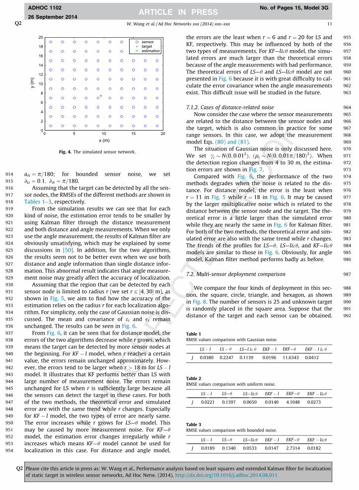
The algorithms described above are implemented inMATLAB to evaluate their performance and make compar-ison. The simulated sensor network, which is shown inFig. 4, consists of N ¼ 100 nodes that are well-distributedon a square area of 20 m � 20 m. A random unknown tar-get is placed in this area, then we use the measurementsof sensor nodes to estimate the target’s position and calcu-late the root mean squared errors (RMSE) via Monte Carlosimulations:

J ¼ 1M

XM

m¼1

ffiffiffiffiffiffiffiffiffiffiffiffiffiffiffiffiffiffiffiffiffiffiffiffiffiffiffiffiffiffiffiffiffiffiffiffiffiffiffiffiffiffiffiffiffiffiffiffiffiffiffiffiffiffiffiffiffiffiffiffiffiffiffiffiffiffixðmÞ � xtrueð Þ2 þ yðmÞ � ytrueð Þ2

h irð133Þ

where ðxtrue; ytrueÞ is the true position of the node, ðxðmÞ; yðmÞÞis the position estimate in the mth simulation, and M is thetotal number of random simulations. In our simulations,we take M = 10,000.

7.1.1. Cases of distance-unrelated noiseIn the case of Gaussian sensor noise, we set rLi ¼ 0:1;

rhi ¼ p=180; for uniform sensor noise, we set aLi ¼ 0:1;



914

915

916

917

918

919

920

921

922

923

924

925

926

927

928

929

930

931

932

933

934

935

936

937

938

939

940

941

942

943

944

945

946

947

948

949

950

951

952

953

954

955

956

957

958

959

960

961

962

963

964

965

966

967

968

969

970

971

972

973

974

975

976

977

978

979

980

981

982

983

984

985

986

987

988

989

990

991

992

0 5 10 15 200

2

4

6

8

10

12

14

16

18

20

x (m)

y (m

)

sensortargetestimation

Fig. 4. The simulated sensor network.

Table 1RMSE values comparison with Gaussian noise.

LS� l LS� h LS—l & h EKF � l EKF—h EKF � l & h

J 0.0380 0.2247 0.1139 0.0196 11.6343 0.0412

Table 2RMSE values comparison with uniform noise.

LS� l LS—h LS—l&h EKF � l EKF—h EKF � l&h

J 0.0221 0.1397 0.0650 0.0140 4.1048 0.0273

Table 3RMSE values comparison with bounded noise.

LS� l LS—h LS—l&h EKF � l EKF—h EKF � l&h

J 0.0189 0.1340 0.0533 0.0147 2.7314 0.0182



26 September 2014

Q2

ahi ¼ p=180; for bounded sensor noise, we setdLi ¼ 0:1; dhi ¼ p=180.

Assuming that the target can be detected by all the sen-sor nodes, the RMSEs of the different methods are shown inTables 1–3, respectively.

From the simulation results we can see that for eachkind of noise, the estimation error tends to be smaller byusing Kalman filter through the distance measurementand both distance and angle measurements. When we onlyuse the angle measurement, the results of Kalman filter areobviously unsatisfying, which may be explained by somediscussions in [50]. In addition, for the two algorithms,the results seem not to be better even when we use bothdistance and angle information than single distance infor-mation. This abnormal result indicates that angle measure-ment noise may greatly affect the accuracy of localization.

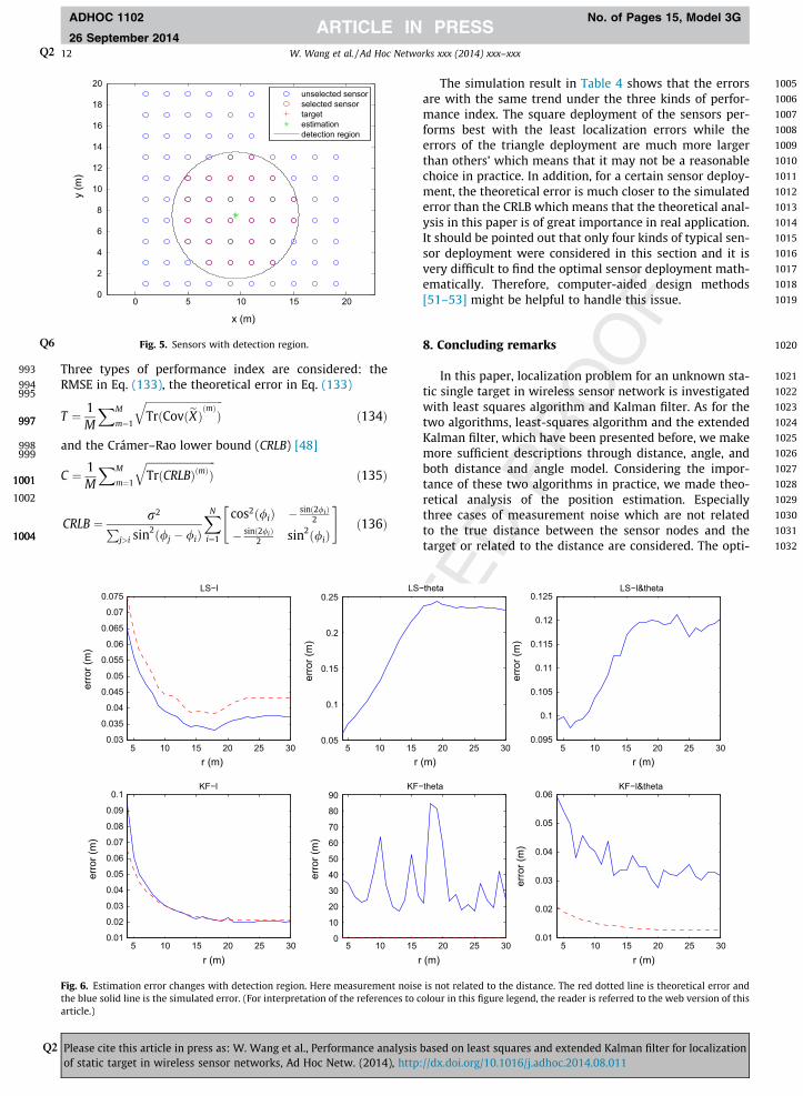
Assuming that the region that can be detected by eachsensor node is limited to radius r (we set r 2 ½4;30�m), asshown in Fig. 5, we aim to find how the accuracy of theestimation relies on the radius r for each localization algo-rithm. For simplicity, only the case of Gaussian noise is dis-cussed. The mean and covariance of ei and �i remainunchanged. The results can be seen in Fig. 6.

From Fig. 6, it can be seen that for distance model, theerrors of the two algorithms decrease while r grows, whichmeans the target can be detected by more sensor nodes atthe beginning. For KF � l model, when r reaches a certainvalue, the errors remain unchanged approximately. How-ever, the errors tend to be larger when r > 18 m for LS� lmodel. It illustrates that KF performs better than LS withlarge number of measurement noise. The errors remainunchanged for LS when r is sufficiently large because allthe sensors can detect the target in these cases. For bothof the two methods, the theoretical error and simulatederror are with the same trend while r changes. Especiallyfor KF � l model, the two types of error are nearly same.The error increases while r grows for LS—h model. Thismay be caused by more measurement noise. For KF—hmodel, the estimation error changes irregularly while rincreases which means KF—h model cannot be used forlocalization in this case. For distance and angle model,


the errors are the least when r ¼ 6 and r ¼ 20 for LS andKF, respectively. This may be influenced by both of thetwo types of measurements. For KF—l&h model, the simu-lated errors are much larger than the theoretical errorsbecause of the angle measurements with bad performance.The theoretical errors of LS—h and LS—l&h model are notpresented in Fig. 6 because it is with great difficulty to cal-culate the error covariance when the angle measurementsexist. This difficult issue will be studied in the future.

7.1.2. Cases of distance-related noiseNow consider the case where the sensor measurements

are related to the distance between the sensor nodes andthe target, which is also common in practice for somerange sensors. In this case, we adopt the measurementmodel Eqs. (80) and (81).

The situation of Gaussian noise is only discussed here.We set ci � Nð0;0:012Þ; ðli � Nð0;0:01p=180Þ2Þ. Whenthe detection region changes from 4 to 30 m, the estima-tion errors are shown in Fig. 7.

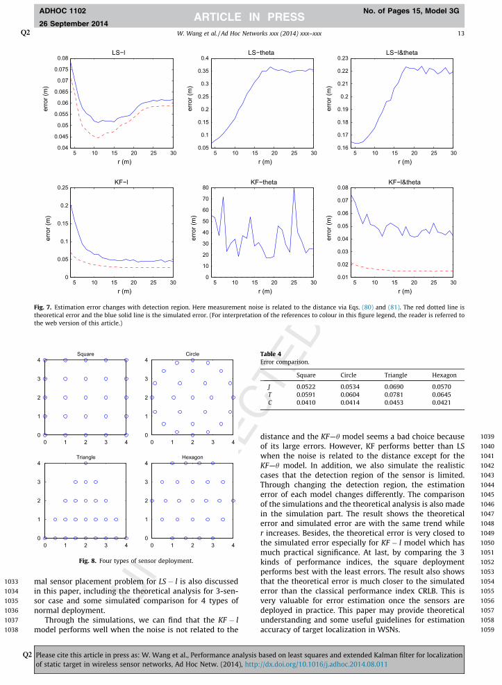
Compared with Fig. 6, the performance of the twomethods degrades when the noise is related to the dis-tance. For distance model, the error is the least whenr ¼ 11 in Fig. 5 while r ¼ 18 in Fig. 6. It may be causedby the larger multiplicative noise which is related to thedistance between the sensor node and the target. The the-oretical error is a little larger than the simulated errorwhile they are nearly the same in Fig. 6 for Kalman filter.For both of the two methods, the theoretical error and sim-ulated error are also with the same trend while r changes.The trends of the profiles for LS—h; LS—l&h, and KF—l&hmodels are similar to those in Fig. 6. Obviously, for anglemodel, Kalman filter method performs badly as before.

7.2. Multi-sensor deployment comparison

We compare the four kinds of deployment in this sec-tion, the square, circle, triangle, and hexagon, as shownin Fig. 8. The number of sensors is 25 and unknown targetis randomly placed in the square area. Suppose that thedistance of the target and each sensor can be obtained.



993

994995

997997

998999

10011001

1002

10041004

1005

1006

1007

1008

1009

1010

1011

1012

1013

1014

1015

1016

1017

1018

1019

1020

1021

1022

1023

1024

1025

1026

1027

1028

1029

1030

1031

0 5 10 15 200

2

4

6

8

10

12

14

16

18

20

x (m)

y (m

)

unselected sensorselected sensortargetestimationdetection region

Fig. 5. Sensors witQ6 h detection region.



26 September 2014

Q2

Three types of performance index are considered: theRMSE in Eq. (133), the theoretical error in Eq. (133)

T ¼ 1M

XM

m¼1

ffiffiffiffiffiffiffiffiffiffiffiffiffiffiffiffiffiffiffiffiffiffiffiffiffiffiffiffiffiffiTrðCovðeXÞðmÞÞq

ð134Þ

and the Crámer–Rao lower bound (CRLB) [48]

C ¼ 1M

XM

m¼1

ffiffiffiffiffiffiffiffiffiffiffiffiffiffiffiffiffiffiffiffiffiffiffiffiffiffiffiTrðCRLBÞðmÞÞ

qð135Þ

CRLB ¼ r2Pj>i sin2ð/j � /iÞ

XN

i¼1

cos2ð/iÞ � sinð2/iÞ2

� sinð2/iÞ2 sin2ð/iÞ

" #ð136Þ

5 10 15 20 25 300.03

0.035

0.04

0.045

0.05

0.055

0.06

0.065

0.07

0.075LS−l

r (m)

erro

r (m

)

5 10 150.05

0.1

0.15

0.2

0.25LS

r

erro

r (m

)

5 10 15 20 25 300.01

0.02

0.03

0.04

0.05

0.06

0.07

0.08

0.09

0.1KF−l

r (m)

erro

r (m

)

5 10 150

10

20

30

40

50

60

70

80

90KF

r

erro

r (m

)

Fig. 6. Estimation error changes with detection region. Here measurement noisethe blue solid line is the simulated error. (For interpretation of the references to carticle.)


The simulation result in Table 4 shows that the errorsare with the same trend under the three kinds of perfor-mance index. The square deployment of the sensors per-forms best with the least localization errors while theerrors of the triangle deployment are much more largerthan others’ which means that it may not be a reasonablechoice in practice. In addition, for a certain sensor deploy-ment, the theoretical error is much closer to the simulatederror than the CRLB which means that the theoretical anal-ysis in this paper is of great importance in real application.It should be pointed out that only four kinds of typical sen-sor deployment were considered in this section and it isvery difficult to find the optimal sensor deployment math-ematically. Therefore, computer-aided design methods[51–53] might be helpful to handle this issue.

1032

8. Concluding remarks

In this paper, localization problem for an unknown sta-tic single target in wireless sensor network is investigatedwith least squares algorithm and Kalman filter. As for thetwo algorithms, least-squares algorithm and the extendedKalman filter, which have been presented before, we makemore sufficient descriptions through distance, angle, andboth distance and angle model. Considering the impor-tance of these two algorithms in practice, we made theo-retical analysis of the position estimation. Especiallythree cases of measurement noise which are not relatedto the true distance between the sensor nodes and thetarget or related to the distance are considered. The opti-

20 25 30

−theta

(m)5 10 15 20 25 30

0.095

0.1

0.105

0.11

0.115

0.12

0.125LS−l&theta

r (m)

erro

r (m

)

20 25 30

−theta

(m)5 10 15 20 25 30

0.01

0.02

0.03

0.04

0.05

0.06KF−l&theta

r (m)

erro

r (m

)

is not related to the distance. The red dotted line is theoretical error andolour in this figure legend, the reader is referred to the web version of this



1033

1034

1035

1036

1037

1038

1039

1040

1041

1042

1043

1044

1045

1046

1047

1048

1049

1050

1051

1052

1053

1054

1055

1056

1057

1058

1059

5 10 15 20 25 300.04

0.045

0.05

0.055

0.06

0.065

0.07

0.075

0.08LS−l

r (m)

erro

r (m

)

5 10 15 20 25 300.05

0.1

0.15

0.2

0.25

0.3

0.35

0.4LS−theta

r (m)

erro

r (m

)

5 10 15 20 25 300.16

0.17

0.18

0.19

0.2

0.21

0.22

0.23LS−l&theta

r (m)

erro

r (m

)

5 10 15 20 25 300

0.05

0.1

0.15

0.2

0.25KF−l

r (m)

erro

r (m

)

5 10 15 20 25 300

10

20

30

40

50

60

70

80KF−theta

r (m)

erro

r (m

)

5 10 15 20 25 300.01

0.02

0.03

0.04

0.05

0.06

0.07

0.08KF−l&theta

r (m)

erro

r (m

)

Fig. 7. Estimation error changes with detection region. Here measurement noise is related to the distance via Eqs. (80) and (81). The red dotted line istheoretical error and the blue solid line is the simulated error. (For interpretation of the references to colour in this figure legend, the reader is referred tothe web version of this article.)

0 1 2 3 40

1

2

3

4Square

0 1 2 3 40

1

2

3

4Circle

0 1 2 3 40

1

2

3

4Triangle

0 1 2 3 40

1

2

3

4Hexagon

Fig. 8. Four types of sensor deployment.

Table 4Error comparison.

Square Circle Triangle Hexagon

J 0.0522 0.0534 0.0690 0.0570T 0.0591 0.0604 0.0781 0.0645C 0.0410 0.0414 0.0453 0.0421



26 September 2014

Q2

mal sensor placement problem for LS� l is also discussedin this paper, including the theoretical analysis for 3-sen-sor case and some simulated comparison for 4 types ofnormal deployment.

Through the simulations, we can find that the KF � lmodel performs well when the noise is not related to the


distance and the KF—h model seems a bad choice becauseof its large errors. However, KF performs better than LSwhen the noise is related to the distance except for theKF—h model. In addition, we also simulate the realisticcases that the detection region of the sensor is limited.Through changing the detection region, the estimationerror of each model changes differently. The comparisonof the simulations and the theoretical analysis is also madein the simulation part. The result shows the theoreticalerror and simulated error are with the same trend whiler increases. Besides, the theoretical error is very closed tothe simulated error especially for KF � l model which hasmuch practical significance. At last, by comparing the 3kinds of performance indices, the square deploymentperforms best with the least errors. The result also showsthat the theoretical error is much closer to the simulatederror than the classical performance index CRLB. This isvery valuable for error estimation once the sensors aredeployed in practice. This paper may provide theoreticalunderstanding and some useful guidelines for estimationaccuracy of target localization in WSNs.



1060

10611062106310641065106610671068106910701071107210731074107510761077107810791080108110821083108410851086108710881089109010911092109310941095109610971098109911001101110211031104110511061107110811091110111111121113111411151116111711181119112011211122112311241125112611271128112911301131113211331134113511361137

1138113911401141114211431144114511461147114811491150115111521153115411551156115711581159116011611162116311641165116611671168116911701171117211731174117511761177117811791180118111821183118411851186118711881189119011911192119311941195119611971198119912001201120212031204120512061207120812091210121112121213121412151216



26 September 2014

Q2

References

[1] I.F. Akyildiz, W. Su, Y. Sankarasubramaniam, E. Cayirci, A survey onsensor networks, IEEE Commun. Mag. 40 (2002) 104–112.

[2] J. Yick, B. Mukherjee, D. Ghosal, Wireless sensor network survey,Comput. Netw. 52 (2008) 2292–2330.

[3] S.K. Teh, L. Mejias, P. Corke, W. Hu, Experiments in integratingautonomous uninhabited aerial vehicles (UAVs) and wireless sensornetworks, in: Australasian Conference on Robotics and Automation(ACRA 08), December 2008.

[4] T. Bokareva, W. Hu, S. Kanhere, Wireless sensor networks forbattlefield surveillance, in: Proceedings of The Land WarfareConference (LWC), 2006.

[5] Y.K. Toh, W. Xiao, L. Xie, A wireless sensor network target trackingsystem with distributed competition based sensor scheduling, in:3rd International Conference on Intelligent Sensors, SensorNetworks and Information, December 2007, pp. 257–262.

[6] V. Bhuse, A. Gupta, Anomaly intrusion detection in wireless sensornetworks, J. High Speed Netw. 15 (2006) 33–51.

[7] M. Bahrepour, N. Meratnia, M. Poel, Z. Taghikhaki, P.J.M. Havinga,Distributed event detection in wireless sensor networks for disastermanagement, in: 2010 2nd International Conference on IntelligentNetworking and Collaborative Systems (INCOS), 2010, pp. 507–512.

[8] A. Redondi, M. Chirico, L. Borsani, M. Cesana, M. Tagliasacchi, Anintegrated system based on wireless sensor networks for patientmonitoring, localization and tracking, Ad Hoc Netw. 11 (2013) 39–53.

[9] R.J. Huang, W.Z. Song, M.S. Xu, N. Peterson, B.A. Shirazi, R. LaHusen,Real-world sensor network for long-term volcano monitoring:design and findings, IEEE Trans. Parall. Distrib. Syst. 23 (2012)321–329.

[10] R. Tan, G.L. Xing, J.Z. Chen, W.Z. Song, R.J. Huang, Quality-drivenvolcanic earthquake detection using wireless sensor networks, in:IEEE 31st Real-Time Systems Symposium (RTSS), December 2010,pp. 271–280.

[11] A. Pal, Localization algorithms in wireless sensor networks: currentapproaches and future challenges, Netw. Protoc. Algor. 2 (1) (2010)45–74.

[12] L. Doherty, L.E. Ghaoui, K.S.J. Pister, Convex position estimation inwireless sensor networks, in: Proceedings of Infocom 2001,Anchorage, AK 3, April 2001, pp. 1655–1663.

[13] J. Hightower, G. Boriello, Location systems for ubiquitous computing,Computer 34 (8) (2001) 57–66.

[14] J. Bachrach, C. Taylor, Localization in sensor networks, HandbookSens. Netw.: Algor. Architect. (2005).

[15] G.Q. Mao, B. Fidan, B.D.O. Anderson, Wireless sensor networklocalization techniques, Comput. Netw. 51 (2007) 2529–2553.

[16] T. Alhmiedat, S.H. Yang, A survey: localization and tracking mobiletargets through wireless sensors network, in: Proceedings of 2007PGNet, 2007, pp. 104–112. <http://www.cms.livjm.ac.uk/pgnet2007/Proceedings/Papers/2007-048.pdf>.

[17] B.S. Rao, H.F. Durrant-Whyte, Fully decentralised algorithm formultisensor Kalman fitering, IEE Proc. Contr. Theory Appl. 138(1991) 413–420.

[18] M. Sun, L. Yang, K.C. Ho, Accurate sequential self-localization ofsensor nodes in closed-form, Signal Process. 92 (2012) 2940–2951.

[19] X. Cheng, A. Thaeler, G. Xue, D. Chen, TPS: a time-based positioningscheme for outdoor wireless sensor networks, in: Proceedings ofIEEE INFOCOM’04, vol. 4, 2004.

[20] F.M. Han, W.Y. Leong, Investigating target detection and localizationin wireless sensor network, Proc. Eng. 41 (2012) 75–81.

[21] R. Peng, M.L. Sichitiu, Angle of arrival localization for wireless sensornetworks, in: 3rd Annual IEEE Communications Society on Sensorand Ad Hoc Communications and Networks, 2006.

[22] T. He, C.D. Huang, B.M. Blum, J.A. Stankovic, Range-free localizationschemes for large scale sensor networks, in: Proceedings of the 9thAnnual International Conference on Mobile Computing andNetworking, September 2003, pp. 81–95.

[23] Y. Wang, X.D. Wang, D.M. Wang, D.P. Agrawal, Range-freelocalization using expected hop progress in wireless sensornetworks, IEEE Trans. Parall. Distrib. Syst. 20 (2009) 1540–1552.

[24] Z. Chaczko, R. Klempous, J. Nikodem, M. Nikodem, Methods of sensorlocalization in wireless sensor networks, in: Proceedings of the 14thAnnual IEEE International Conference and Workshops on theEngineering of Computer-Based Systems, March 2007, pp. 145–152.

[25] F.K.W. Chan, H.C. So, Accurate sequential weighted least squaresalgorithm for wireless sensor network localization, in: 14thEuropean Signal Proceeding Conference (EUSIPCO 2006),September 2006, pp. 104–112.


[26] R. Behnke, J. Salzmann, D. Lieckfeldt, D. Timmermann, SDLS -distributed least squares localization for large wireless sensornetworks, in: ICUMT’09 International Conference on Ultra ModernTelecommunications and Workshops, 2009, pp. 1–6.

[27] H.C. So, L. Lin, Linear least squares approach for accurate receivedsignal strength based source localization, IEEE Trans. Signal Process.59 (8) (2011) 4035–4040.

[28] C.-H. Park, K.-S. Hong, Block LMS-based source localization usingrange measurement, Digit. Signal Process. 21 (2011) 367–374.

[29] K. Yu, 3-D localization error analysis in wireless networks, IEEETrans. Wirel. Commun. 6 (10) (2007) 3473–3481.

[30] J.M. Chen, C.Q. Wang, Y.X. Sun, X.M. Shen, Semi-supervised Laplacianregularized least squares algorithm for localization in wirelesssensor networks, Comput. Netw. 55 (2011) 2481–2491.

[31] Christof, M. Mller, Localization of sensor nodes in a wireless sensornetwork using the nanaLOC TRX transceiver, Comput. Netw. 52(2008) 2292–2330.

[32] Y.S. Yan, H.Y. Wang, W. Xuan, A novel least-square method of sourcelocalization based on acoustic energy measurements for UWSN, in:IEEE International Conference on Communications and Computing(ICSPCC), September 2011.

[33] A. Born, F. Reichenbach, Converting the nonlinear least squaresproblem for localization in wireless sensor networks, in: Proceedingsof 19th International Conference on Computer Communications andNetworks (ICCCN), 2010.

[34] B. Seet, Q. Zhang, C. Foh, A. Fong, Hybrid RF mapping and Kalmanfiltered spring relaxation for sensor network localization, IEEE Sens.J. 1 (1) (2010).

[35] Y. Zhang, S.T. Liu, X.Y. Zhao, Z.T. Jia, Theoretic analysis of uniquelocalization for wireless sensor networks, Ad Hoc Netw. 10 (2012)622–634.

[36] C. Cheng, S. Anant, Estimation bounds for localization, in: 2004 FirstAnnual IEEE Communications Society Conference on sensor and AdHoc Communications and Networks, 2004, pp. 415–424.

[37] S. Zhang, J. Cao, Y. Zeng, Z. Li, On accuracy of region basedlocalization algorithms for wireless sensor networks, Comput.Commun. 33 (12) (2010) 1391–1403.

[38] B. Huang, C. Yu, B.D.O. Anderson, Analyzing localization errors inone-dimensional sensor networks, Signal Process. 92 (2012) 427–438.

[39] W. Meng, L.H. Xie, W.D. Xiao, Sensor placement in heterogeneoussensor networks, in: 2012 12th International Conference on Control,Automation, Robotics & Vision, Guangzhou, China, 2012, pp. 684–689.

[40] J.Y. Zhou, J. Shi, Error analysis of non-collaborative wirelesslocalization in circular-shaped regions, Comput. Netw. 54 (2010)2439–2452.

[41] W.D. Wang, H.B. Ma, Y.Q. Wang, M.Y. Fu, Localization of static targetin WSNs with least-squares and extended Kalman filter, in: 201212th International Conference on Control, Automation, Robotics &Vision, Guangzhou, China, 2012, pp. 602–607.

[42] M. Takruri, S. Rajasegarar, S. Challa, C. Leckie, M. Palaniswami,Online drift correction in wireless sensor networks using spatio-temporal modelling, in: Proceedings of the 11th InternationalConference on Information Fusion (Fusion 2008), Cologne,Germany, July 2008.

[43] M. Takruri, S. Challa, R. Chakravorty, Recursive bayesian approachesfor auto calibration in drift aware wireless sensor networks, J. Netw.5 (7) (2010) 823–832.

[44] M. Takruri, S. Rajasegarar, S. Challa, C. Leckie, Spatio-temporalmodelling based drift aware wireless sensor networks, IET Wirel.Sens. Syst. 1 (2) (2011) 110–122.

[45] S.M. Stigler, The History of Statistics: The Measurement ofUncertainty Before 1900, Belknap Press of Harvard UniversityPress, Cambridge, MA, 1986.

[46] R.E. Kalman, R.S. Bucy, New results in linear filtering and predictiontheory, Trans. ASME. Ser. D, J. Basic Eng. 83 (1961) 95–107.

[47] S.F. Schmidt, The Kalman filter: its recognition and development foraerospace applications, AIAA J. Guid. Contr. 4 (1) (1981) 4–7.

[48] A.N. Bishop, B. Fidan, B.D.O. Anderson, K. Dog�ancay, P.N. Pathirana,Optimality analysis of sensor-target localization geometries,Automatica 46 (2010) 479–492.

[49] X.B. Wang, M.Y. Fu, H.S. Zhang, Target tracking in wirelesssensor networks based on the combination of KF and MLE usingdistance measurements, IEEE Trans. Mobile Comput. 11 (2012) 567–576.

[50] D.F. Bizup, D.E. Brown, The over-extended Kalman filter - don’t useit! in: Proceedings of the Sixth International Conference onInformation Fusion, Cairns, Qld., Australia: Univ. New Mexico,2003, pp. 227–233.


http://www.cms.livjm.ac.uk/pgnet2007/Proceedings/Papers/2007-048.pdf

http://www.cms.livjm.ac.uk/pgnet2007/Proceedings/Papers/2007-048.pdf


1217121812191220122112221223122412251226

1227

12291229

123012311232123312341235123612371238

12401240

124112421243124412451246124712481249125012511252

12541254

12551256125712581259126012611262126312641265126612671268126912701271127212731274

1277Q512781279128012811282



26 September 2014

Q2

[51] G. Xu, B. Mourrain, R. Duvigneau, A. Galligo, Constructing analysis-suitable parameterization of computational domain from CADboundary by variational harmonic method, J. Comput. Phys. 252(2013) 275–289.

[52] G. Xu, B. Mourrain, R. Duvigneau, A. Galligo, Optimal analysis-awareparameterization of computational domain in 3D isogeometricanalysis, Comput. Aided Des. 45 (2013) 812–821.

[53] G. Xu, B. Mourrain, R. Duvigneau, A. Galligo, Analysis-suitablevolume parameterization of multi-block computational domain inisogeometric applications, Comput. Aided Des. 252 (2013) 395–404.

Weidong Wang Master candidate at the Col-lege of Information Science and Technology,Beijing University of Chemical Technology. Hereceived his bachelor degree from BeijingUniversity of Chemical Technology in 2011.His research interest covers localization inwireless sensor networks and filtering tech-niques as well as their applications.

12761276

12831284128512861287

Hongbin Ma Professor at the School of Auto-mation, Beijing Institution of Technology. Hereceived his bachelor degree from ZhengzhouUniversity in 2001 and doctoral degree fromthe Academy of Mathematics and SystemsScience, Chinese Academy of Sciences in 2006.His research focuses on adaptation, learningand recognition, especially adaptive estima-tion and control, as well as their applications.He is also a member of IEEE, ACM and SIAM.Corresponding author of this paper.


Youqing Wang Professor at the College ofInformation Science and Technology, BeijingUniversity of Chemical Technology. receivedthe B.S. degree from Shandong University,Jinan, Shandong, China, in 2003, and the Ph.D.degree in control science and engineeringfrom Tsinghua University, Beijing, China, in2008. His current research interests includemodeling and control of biomedical processes(e.g., artificial pancreas system, anesthesia),health informatics, batch processes, iterativelearning control, model predictive control,

and fault-tolerant control. Dr. Wang is in the editorial board of Mathe-matical Problems in Engineering and ISRN Applied Mathematics. He is amember of the International Federation of Automatic Control Technical
Committee on Biological and Medical Systems. He is the recipient ofseveral research awards (including New Century Excellent Talents inUniversity, the Journal of Process Control Survey Paper Prize and theZhang Zhong-Jun Academician Outstanding Paper Award).
Mengyin Fu Professor Cheung Kong ScholarsProgram, the leader of a program for Chang-jiang Scholars and innovation team, the leaderof an innovation team of national defensescience and technology industry, Professor atthe School of Automation, Beijing Institutionof Technology. His research focuses on inte-grated navigation, intelligent navigation,image processing, learning and recognition aswell as their applications.



Documents

Performance analysis based on least squares and extended Kalman filter for localization of static target in wireless sensor networks